International Journal of Solids and Structures 49 (2012) 420–435

Contents lists available at SciVerse ScienceDirect

International Journal of Solids and Structures

journal homepage: www.elsevier .com/locate / i jsolst r

On the use of simulated experiments in designing tests for materialcharacterization from full-field measurements

Marco Rossi ⇑, Fabrice PierronLMPF, Arts et Métiers ParisTech, Rue St Dominique, B.P. 508, 51006 Châlons-en-Champagne, France

a r t i c l e i n f o a b s t r a c t

Article history:Received 4 May 2010Received in revised form 2 May 2011Available online 19 November 2011

Keywords:Simulated experimentsFull-field measurementsMaterial characterizationTest optimization

0020-7683/$ - see front matter � 2011 Elsevier Ltd. Adoi:10.1016/j.ijsolstr.2011.09.025

⇑ Corresponding author.E-mail addresses: marco.rossi@ensam.eu (M. Ros

ensam.fr (F. Pierron).

The present paper deals with the use of simulated experiments to improve the design of an actualmechanical test. The analysis focused on the identification of the orthotropic properties of compositesusing the unnotched Iosipescu test and a full-field optical technique, the grid method. The experimentaltest was reproduced numerically by finite element analysis and the recording of deformed grey levelimages by a CCD camera was simulated trying to take into account the most significant parameters thatcan play a role during an actual test, e.g. the noise, the failure of the specimen, the size of the grid printedon the surface, etc. The grid method then was applied to the generated synthetic images in order toextract the displacement and strain fields and the Virtual Fields Method was finally used to identifythe material properties and a cost function was devised to evaluate the error in the identification. Thedeveloped procedure was used to study different features of the test such as the aspect ratio and the fibreorientation of the specimen, the use of smoothing functions in the strain reconstruction from noisy data,the influence of missing data on the identification. Four different composite materials were consideredand, for each of them, a set of optimized design variables was found by minimization of the cost function.

� 2011 Elsevier Ltd. All rights reserved.

1. Introduction

The characterization of the mechanical properties of materialsby experimental tests is one of the important issues in engineer-ing. Depending on the type of material and the property to deter-mine, many different tests have been devised during the years,some of which have become standards in industrial practice.Looking at mechanical properties, such as elastic modulus, Pois-son’s ratio, yield strength, toughness, damage, etc., the experi-mental procedure usually consists in submitting a specimen todifferent loading conditions and measuring the applied forceand specimen deformation. Examples of this kind of experimentsare tensile tests, upsetting tests, shear tests, punch tests, bulgetests, etc. When the material behaviour is more complex and sev-eral parameters must be identified in the constitutive equation, asoccurs for instance in composites, anisotropic metals or rubbers,the characterization becomes more difficult and multiple testshave to be used.

Recently, the improvement in full-field measurement tech-niques and digital camera performances has led to the design ofnovel test procedures (Avril et al., 2008a; Grédiac, 2004). The idea

ll rights reserved.

si), Fabrice.Pierron@chalons.

is to use a test configuration that induces heterogeneous stress andstrain fields in the specimen so that more parameters of thematerial constitutive equations can be activated at the same time.The full-field measurement technique is employed to measure thedisplacement field of the specimen surface. At this point, the mea-sured data are used to identify the material properties by inverseapproaches, e.g. the finite element updating method (Cooremanet al., 2008; Lecompte et al., 2007; Le Magorou et al., 2002;Meuwissen et al., 1998; Kajberg and Lindkvist, 2004), the constitu-tive equation gap method (Latourte et al., 2008; Geymonat andPagano, 2003), the equilibrium gap method (Claire et al., 2004),the reciprocity gap method (Bui et al., 2004) or other techniques(Rossi et al., 2008).

An alternative is the Virtual Fields Method (VFM) which is awell established technique to characterize the material propertiesdirectly from full-field measurements (Grédiac et al., 2006). Anumber of different applications have already been considered inpast studies, e.g. the elastic stiffness of composites (Grédiac andVautrin, 1990; Moulart et al., 2006), damping measurements onvibrating plates (Giraudeau and Pierron, 2005), elasto-plasticity(Grédiac and Pierron, 2006) etc.

The pattern of the displacement field generated by the experi-ment and the optical technique adopted to measure it play animportant role in the final identification of the parameters. Theintention of this paper is to develop a procedure to design an

M. Rossi, F. Pierron / International Journal of Solids and Structures 49 (2012) 420–435 421

optimized test configuration for a given class of materials and typeof test. This has scarcely been addressed in the literature(Le Magorou et al., 2002; Pierron et al., 2007; Syed-Muhammadet al., 2009) and a lot of improvements can still be made in thisfield.

The best configuration comes from the minimization of a costfunction that represents the average error in the identification asa function of the design variables. It is not practically feasible touse real experiments in the optimization process because of thegreat amount of different configurations that have to be testedand the difficulty of controlling the experimental conditions. Forthis reason the experiments have been simulated using a combina-tion of FE models and data post-processing. A great attention isnecessary on reproducing real experiments to avoid the presenceof numerical artifacts that could lead to unexpected results. Similarprocedures were already used, for instance, to assess the error indigital image correlation measurements with simulated white-light speckle patterns (Bornert et al., 2009).

In this paper, the study focused on the unnotched Iosipescutest (Pierron and Grédiac, 2000) used to determine the constitu-tive parameters of orthotropic materials such as carbon or glassepoxy composites. The four in-plane stiffness components canbe determined from one test using the VFM. A first attempt tooptimize the test configuration of a Iosipescu test was addressedin a previous paper by Pierron et al. (2007) where the sensitivityto noise was used as the variable to minimize a cost function.Although an improvement in the quality of the identificationwas obtained, some limitations were noticed in such an approach.Mainly, the optimization procedure did not include the effect ofthe spatial resolution of the measurement technique, besides,only one source of error was considered, the uncorrelated whitenoise on the strain field.

The present work represents a continuation and an extension ofthat study. In order to overcome the mentioned limitations, the in-tent here is trying to numerically reproduce the whole measure-ment process as accurately as possible. Synthetic images weregenerated to simulate a real acquisition with a CCD camera andthe noise was applied directly to the grey level images. A full-fieldtechnique, the grid method, was used to extract the strain fieldfrom the images and the data were used to identify the parameterswith the VFM. In this way the effect of the spatial resolution isintroduced and the influence of noise is more realistic.

The developed procedure gives a versatile tool to study andoptimize an experimental setup and several practical aspects canbe efficiently evaluated, for instance the effect of smoothing proce-dures to derive the strains from the displacements or the influenceof missing data, two very important practical features. Moreoverthe same procedure could be easily extended to take into accountother important aspects like the existence of optical distortions orthe pixel fill factor.

To the best knowledge of the authors, this is the first time thatthe whole measurement and identification chain is simulated andused to optimize a test configuration.

2. Description of the techniques used in the simulatedexperiments

The identification process is based on two specific techniques,the grid method, used to measure a two-dimensional displacementfield on a loaded specimen, and the Virtual Fields Method, used toidentify the material properties from full-field measurements. Anin-depth treatment of the subject can be found in the cited refer-ences, nevertheless a brief description of the methods is given be-low to provide a background for the reader and produce a betterunderstanding of the following sections.

2.1. The grid method

The grid method is a full-field optical technique that allows tomeasure the displacement field on a specimen surface with a highresolution and therefore it is particularly suitable for the small dis-placements obtained in the elastic range (Avril et al., 2004a,c;Surrel, 1994).

A grid pattern is printed onto the surface of the specimen usingappropriate techniques (Piro and Grédiac, 2004) and a digital im-age of the surface is achieved using a CCD camera. The intensityof the digitized light at a given pixel M0, that corresponds to thematerial point determined by the position vector R

!ðx; yÞ in thereference cartesian frame, can be expressed by:

Ið R!Þ ¼ I0f1þ c frng½2p F

!� R!�g ð1Þ

where

� I0 is the local intensity bias,� c is the contrast,� frng is a 2p-periodic continuous function,� 2p F

!� R!

is the phase of function frng,� F!

is the spatial frequency vector. It is orthogonal to the gridlines and its amplitude is the spatial frequency of the grid. Ifthe grid lines are vertical (parallel to the y-axis), the spatial fre-quency vector writes F

!ðf0;0Þ. If the grid lines are horizontal, thespatial frequency vector writes F

!ð0; f0Þ.

When a load is applied, the material and consequently the gridare deformed. The phase of the function frng at pixel M0 varies of�2p F

!� u!ð R!Þ from the undeformed to the deformed state, where

u!ð R!Þ is the displacement vector. The ux(x,y) and uy(x,y) displace-

ment components relative to the unloaded reference conditionare calculated from the respective phase differences D/x (forvertical lines) and D/y (for horizontal lines) introduced by thedeformation:

uxðx; yÞ ¼ �p

2pD/xðx; yÞ ð2Þ

uyðx; yÞ ¼ �p

2pD/yðx; yÞ ð3Þ

with p equal to the pitch size of the grid. It has to be pointed outthat the grid method and the computation of the displacementusing Eqs. (2) and (3) is valid only under the hypothesis of small dis-placement. The strain field is obtained consequently by a differenti-ation of the displacement field:

eij ¼12@ui

@xjþ @uj

@xi

� �; i; j 2 ½1—3� ð4Þ

Routines to extract the phase fields by using the spatial phaseshifting method, i.e. the Windowed Discrete Fourier Transform(WDTF) algorithm with a triangular window, have been alreadyimplemented in Matlab and can be directly applied to the digitalimages (Surrel, 1996, 1997). Considering the first harmonic offunction frng, Eq. (1) has three unknowns, so a minimum samplingof 3 pixels per period is necessary. The practical experience dem-onstrated that a good compromise is to have the period p of thegrid sampled by about five pixels. Increasing the number of pixelsper period will reduce the spatial resolution while going under fivepixels will start to deteriorate the phase detection.

Another practical issue is the minimum size of the grid which ispossible to print on the specimen. Although microgrids have beensuccessfully used for measurements at the microscale (Moulartet al., 2007, 2009), in applications at the macroscale level the min-imum grid pitch is around 100 lm (Piro and Grédiac, 2004), whichis the value adopted here. Most of the full-field optical techniques

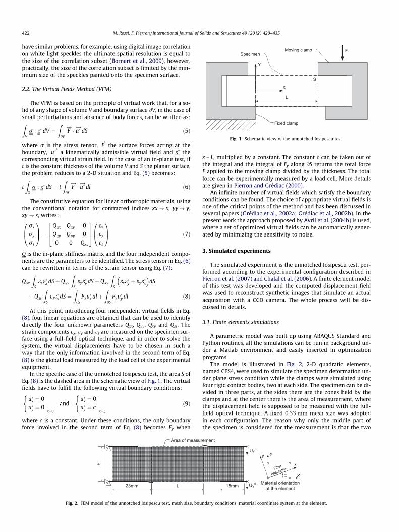
Fig. 1. Schematic view of the unnotched Iosipescu test.

422 M. Rossi, F. Pierron / International Journal of Solids and Structures 49 (2012) 420–435

have similar problems, for example, using digital image correlationon white light speckles the ultimate spatial resolution is equal tothe size of the correlation subset (Bornert et al., 2009), however,practically, the size of the correlation subset is limited by the min-imum size of the speckles painted onto the specimen surface.

2.2. The Virtual Fields Method (VFM)

The VFM is based on the principle of virtual work that, for a so-lid of any shape of volume V and boundary surface @V, in the case ofsmall perturbations and absence of body forces, can be written as:Z

Vr : e� dV ¼

Z@V

F!� u�!dS ð5Þ

where r is the stress tensor, F!

the surface forces acting at theboundary, u�

�!a kinematically admissible virtual field and e⁄ the

corresponding virtual strain field. In the case of an in-plane test, ift is the constant thickness of the volume V and S the planar surface,the problem reduces to a 2-D situation and Eq. (5) becomes:

tZ

Sr : e� dS ¼ t

Z@S

F!� u�!dl ð6Þ

The constitutive equation for linear orthotropic materials, usingthe conventional notation for contracted indices xx ? x, yy ? y,xy ? s, writes:

rx

ry

rs

0B@

1CA ¼ Q xx Qxy 0

Q xy Q yy 00 0 Q ss

264

375 ex

ey

es

0B@

1CA ð7Þ

Q is the in-plane stiffness matrix and the four independent compo-nents are the parameters to be identified. The stress tensor in Eq. (6)can be rewritten in terms of the strain tensor using Eq. (7):

Q xx

ZSexe�x dSþ Q yy

ZSeye�y dSþ Q xy

ZS

exe�y þ eye�x� �

dS

þ Q ss

ZSese�s dS ¼

Z@S

Fxu�x dlþZ@S

Fyu�y dl ð8Þ

At this point, introducing four independent virtual fields in Eq.(8), four linear equations are obtained that can be used to identifydirectly the four unknown parameters Qxx, Qyy, Qxy and Qss. Thestrain components ex, ey and es are measured on the specimen sur-face using a full-field optical technique, and in order to solve thesystem, the virtual displacements have to be chosen in such away that the only information involved in the second term of Eq.(8) is the global load measured by the load cell of the experimentalequipment.

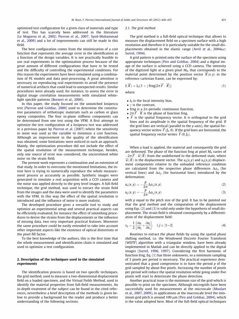
In the specific case of the unnotched Iosipescu test, the area S ofEq. (8) is the dashed area in the schematic view of Fig. 1. The virtualfields have to fulfill the following virtual boundary conditions:

u�x ¼ 0u�y ¼ 0

( �����x¼0

andu�x ¼ 0u�y ¼ c

( �����x¼L

ð9Þ

where c is a constant. Under these conditions, the only boundaryforce involved in the second term of Eq. (8) becomes Fy when

Fig. 2. FEM model of the unnotched Iosipescu test, mesh size, bou

x = L, multiplied by a constant. The constant c can be taken out ofthe integral and the integral of Fy along @S returns the total forceF applied to the moving clamp divided by the thickness. The totalforce can be experimentally measured by a load cell. More detailsare given in Pierron and Grédiac (2000).

An infinite number of virtual fields which satisfy the boundaryconditions can be found. The choice of appropriate virtual fields isone of the critical points of the method and has been discussed inseveral papers (Grédiac et al., 2002a; Grédiac et al., 2002b). In thepresent work the approach proposed by Avril et al. (2004b) is used,where a set of optimized virtual fields can be automatically gener-ated by minimizing the sensitivity to noise.

3. Simulated experiments

The simulated experiment is the unnotched Iosipescu test, per-formed according to the experimental configuration described inPierron et al. (2007) and Chalal et al. (2006). A finite element modelof this test was developed and the computed displacement fieldwas used to reconstruct synthetic images that simulate an actualacquisition with a CCD camera. The whole process will be dis-cussed in details.

3.1. Finite elements simulations

A parametric model was built up using ABAQUS Standard andPython routines, all the simulations can be run in background un-der a Matlab environment and easily inserted in optimizationprograms.

The model is illustrated in Fig. 2, 2-D quadratic elements,named CPS4, were used to simulate the specimen deformation un-der plane stress condition while the clamps were simulated usingfour rigid contact bodies, two at each side. The specimen can be di-vided in three parts, at the sides there are the zones held by theclamps and at the center there is the area of measurement, wherethe displacement field is supposed to be measured with the full-field optical technique. A fixed 0.33 mm mesh size was adoptedin each configuration. The reason why only the middle part ofthe specimen is considered for the measurement is that the two

ndary conditions, material coordinate system at the element.

M. Rossi, F. Pierron / International Journal of Solids and Structures 49 (2012) 420–435 423

other parts (in the clamps) undergo little deformation. Also, mea-suring over the whole length will deteriorate the spatial resolutionbecause of the large aspect ratio of the specimen.

The rigid bodies on the left side are fixed while a vertical dis-placement U0

Y is given to the rigid bodies on the right to simulatethe shear loading. A friction coefficient l = 0.05 is used in the con-tact properties to prevent sliding in the horizontal direction. Theapplied force F is obtained as sum of the vertical reactions of therigid bodies at the right.

Two systems of cartesian coordinates are introduced, the refer-ence global coordinate system ð0; X

!; Y!Þ, fixed, and the material

coordinate system ð0; x!; y!Þ in which the x-axis is aligned withthe fibre orientation. The angle a measures the rotation of thematerial coordinate system with respect to the global one and isthe first design variable. The second is the free length of the spec-imen L, illustrated in Fig. 2.

All the other geometric parameters are kept constants, theheight H is set equal to 20 mm and the part of the specimengrabbed by the clamps measures 23 mm. The reason for this choiceis that the fixture can only accommodate a fixed width whereas itcan be used for different free lengths (Pierron, 1994).

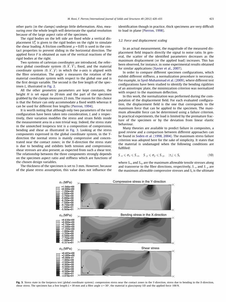
It is worth noting that although only two parameters of the testconfiguration have been taken into consideration, L and a respec-tively, their variation modifies the stress and strain fields insidethe measurement area in a non trivial way. Indeed, the stress statein the unnotched Iosipescu test is a composition of compression,bending and shear as illustrated in Fig. 3. Looking at the stresscomponents expressed in the global coordinate system, in the Y-direction the normal stress is mainly compressive and concen-trated near the contact zones; in the X-direction the stress stateis due to bending and exhibits both tension and compression;shear stresses are also present, as expected from such a shear test.The relationship between the three components strongly dependson the specimen aspect ratio and stiffness which are functions ofthe chosen design variables.

The thickness of the specimen is set to 3 mm. However, becauseof the plane stress assumption, this value does not influence the

Fig. 3. Stress state in the Iosipescu test (global coordinate system): compression stressshear stress. The specimen has a free length L = 30 mm and a fibre angle a = 30�, the ma

identification though in practice, thick specimens are very difficultto load in plane (Pierron, 1998).

3.2. Force and displacement scaling

In an actual measurement, the magnitude of the measured dis-placement field impacts directly the signal to noise ratio. In gen-eral, the scatter of the identified parameters decreases as themaximum displacement (or the applied load) increases. This hasbeen observed, for instance, in some experimental results obtainedfor similar applications (Xavier et al., 2007).

In order to compare different specimen configurations, whichexhibit different stiffness, a normalization procedure is necessary.For example, in Syed-Muhammad et al. (2009), where different testconfigurations have been studied to identify the bending rigiditiesof an anisotropic plate, the minimization criterion was normalizedwith respect to the maximum deflection.

In this work, the normalization was performed during the com-putation of the displacement field. For each evaluated configura-tion, the displacement field is the one that corresponds to themaximum force that can be applied to the specimen. The maxi-mum allowable force can be determined using a failure criterion.In practical experiments, the load is limited by the premature frac-ture of the specimen or by the deviation from linear elasticbehaviour.

Many theories are available to predict failure in composites, agood review and a comparison between different approaches canbe found in Soden et al. (1998, 2004). The maximum stress failurecriterion was adopted here for the sake of simplicity. It states thatthe material is undamaged when the following conditions arefulfilled:

S�x 6 rx 6 Sþx; S�y 6 ry 6 Sþy; jssj 6 Ss ð10Þ

where S+x and S+y are the maximum allowable tensile stresses alongand transverse to the fibre directions, respectively, S�x and S�y arethe maximum allowable compressive stresses and Ss is the ultimate

near the contact zones in the Y-direction, stress due to bending in the X-direction,terial is glass/epoxy UD and the applied force 100 N.

424 M. Rossi, F. Pierron / International Journal of Solids and Structures 49 (2012) 420–435

in-plane shear stress. Obviously, the stress tensor is computed inthe material coordinate system.

Although this assumption is quite simplistic, the model iswidely used in practice and even more complex theories utilize itto restrict the elastic range where no damage is observed (Zinovievet al., 1998; Zinoviev et al., 2002). Here it is just used to provide amore physical normalization of the stress and strain levels.

Under the assumption of small displacement and linear elasticbehaviour, the stress and strain fields are proportional to the ap-plied force. If F is the force computed by the FEM as the verticalresultant of the imposed fixed displacement U0

y on the right partof the fixture, the maximum allowable force, according to the fail-ure criterion, is obtained by scaling the FE reaction force by a factork, with

k¼min maxri

x

Sþx

� ;max

rix

S�x

� ;max

riy

Sþy

!;max

riy

S�y

!;max

sis

Ss

� " #

ð11Þ

and rix; ri

y and sis the stress components at each ith Gauss point of

the numerical model and max(�) is the maximum over all the Gausspoints. In the same way, the displacement field corresponding tothe maximum allowable force is then obtained by the same scalingfactor k.

Two different composites have been investigated, glass/epoxyand carbon/epoxy, looking at two different fibre configurations,unidirectional (UD) and 0�/90�, for a total of four materials. Typicalproperties for the materials can be found in various technical orcommercial catalogues, the values used in this work are listed inTable 1. The idea here was to explore the effect of anisotropy onthe optimal configuration.

3.3. Synthetic images

Analytically, a black and white image can be described as a con-tinuous function Ið R

!Þ of the grey level, where R!

is the positionvector of Section 2.1 defined over a spatial domain that representsthe image size. Let us consider Irð R

!Þ as the grey level function forthe reference image and Idð R

!Þ that of the deformed image,distorted according to a given material transformation UM. Thetwo functions can be put in relation using the optical flowconservation:

Idð R!Þ ¼ Ir U�1

M ð R!Þ

� �ð12Þ

In the general case of a displacement field u! the transformationfunction becomes:

UM ¼ R!þ u!ð R

!Þ ð13Þ

The function Irð R!Þ represents, in terms of grey levels, the pat-

tern printed in the specimen surface before deformation starts.For instance, using digital image correlation, the pattern will be a

Table 1Reference properties for four composite materials. Data from www.performance-composites.com (2010). For the glass/epoxy unidirectional, data from Tsai and Hahn(1980).

Glass/epoxy Carbon/epoxy Glass/epoxy Carbon/epoxyUD UD 0/90� 0/90�

Exx (GPa) 40 135 25 70Eyy (GPa) 10 10 25 70Gxy (GPa) 4 5 4 5mxy 0.3 0.3 0.2 0.1S+x (MPa) 1000 1500 440 600S�x (MPa) �600 �1200 �425 �570S+y (MPa) 40 50 440 600S�y (MPa) �100 �250 �425 �570Ss (MPa) 40 70 40 90

series of speckles with random size. An example of speckle simula-tion can be found in Orteu et al. (2006). Working with the gridmethod, the reference image is an equispaced grid which can bedescribed by the following analytical function:

Irð R!Þ¼ I0 1þc cos

2pXp

� þcos

2pYp

� � cos

2pXp

� �cos

2pYp

� ��������

� � �ð14Þ

where I0 and c are the quantities defined in Eq. (1) and R!¼ ðX;YÞ is

expressed in the global coordinate system, j�j is the absolute value.The analytical function for the deformed image is obtained using Eq.(12), UM is computed from Eq. (13) using the displacement from theFE model, scaled according to the normalization proposed in Section3.2.

At this point, two synthetic images are generated digitizing theimage functions Irð R

!Þ and Idð R!Þ. The intent is to reproduce the

acquisition process of a digital camera. In a digital camera, an im-age is projected through a lens onto the photoactive region, whichis usually a matrix of CCD sensors. Every pixel of the recorded im-age corresponds to a CCD sensor of the camera. A CCD sensor is adevice able to accumulate an electric charge proportional to thelight intensity.

Let us consider a pixel M and the area AM which represents theportion of the grid imaged by that pixel. The digital value stored inM is an integer proportional to the average light intensity insidethe area AM. The area AM represents the sensitive part of the pixeland could be varied to simulate different fill factors. In the presentcase, the light intensity is represented by an analytical functionIð R!Þ, so the digital recorded value P(M) can be computed as

follows:

PðMÞ ¼ 1AM

ZAM

Ið R!ÞdS

� ð15Þ

where b�e is the nearest integer to the value computed inside.The integral in Eq. (15) is numerically computed using pixel

supersampling. The function Ið R!Þ is evaluated at Np points inside

the pixel area AM and P(M) is computed as an average value:

PðMÞ ¼ 1Np

XNp

i¼1

Ið R!

iÞ$ ’

ð16Þ

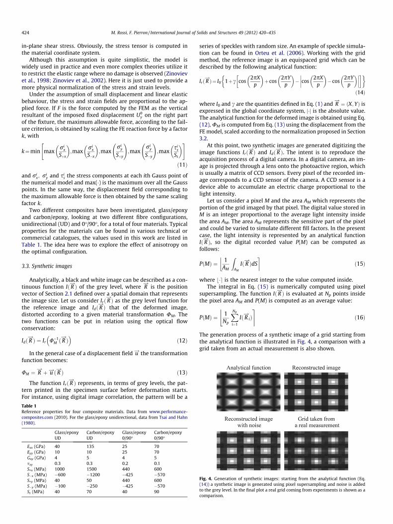
The generation process of a synthetic image of a grid starting fromthe analytical function is illustrated in Fig. 4, a comparison with agrid taken from an actual measurement is also shown.

Fig. 4. Generation of synthetic images: starting from the analytical function (Eq.(14)) a synthetic image is generated using pixel supersampling and noise is addedto the grey level. In the final plot a real grid coming from experiments is shown as acomparison.

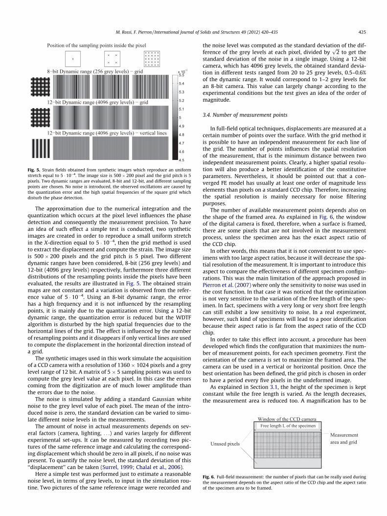
Fig. 5. Strain fields obtained from synthetic images which reproduce an uniformstretch equal to 5 � 10�4. The image size is 500 � 200 pixel and the grid pitch is 5pixels. Two dynamic ranges are evaluated, 8-bit and 12-bit, and different samplingpoints are chosen. No noise is introduced, the observed oscillations are caused bythe quantization error and the high spatial frequencies of the square grid whichdisturb the phase detection.

Fig. 6. Full-field measurement: the number of pixels that can be really used duringthe measurement depends on the aspect ratio of the CCD chip and the aspect ratioof the specimen area to be framed.

M. Rossi, F. Pierron / International Journal of Solids and Structures 49 (2012) 420–435 425

The approximation due to the numerical integration and thequantization which occurs at the pixel level influences the phasedetection and consequently the measurement precision. To havean idea of such effect a simple test is conducted, two syntheticimages are created in order to reproduce a small uniform stretchin the X-direction equal to 5 � 10�4, then the grid method is usedto extract the displacement and compute the strain. The image sizeis 500 � 200 pixels and the grid pitch is 5 pixel. Two differentdynamic ranges have been considered, 8-bit (256 grey levels) and12-bit (4096 grey levels) respectively, furthermore three differentdistributions of the resampling points inside the pixels have beenevaluated, the results are illustrated in Fig. 5. The obtained strainmaps are not constant and a variation is observed from the refer-ence value of 5 � 10�4. Using an 8-bit dynamic range, the errorhas a high frequency and it is not influenced by the resamplingpoints, it is mainly due to the quantization error. Using a 12-bitdynamic range, the quantization error is reduced but the WDTFalgorithm is disturbed by the high spatial frequencies due to thehorizontal lines of the grid. The effect is influenced by the numberof resampling points and it disappears if only vertical lines are usedto compute the displacement in the horizontal direction instead ofa grid.

The synthetic images used in this work simulate the acquisitionof a CCD camera with a resolution of 1360 � 1024 pixels and a greylevel range of 12 bit. A matrix of 5 � 5 sampling points was used tocompute the grey level value at each pixel. In this case the errorscoming from the digitization are of much lower amplitude thanthe errors due to the noise.

The noise is simulated by adding a standard Gaussian whitenoise to the grey level value of each pixel. The mean of the intro-duced noise is zero, the standard deviation can be varied to simu-late different noise levels in the measurements.

The amount of noise in actual measurements depends on sev-eral factors (camera, lighting, . . .) and varies largely for differentexperimental set-ups. It can be measured by recording two pic-tures of the same reference image and calculating the correspond-ing displacement which should be zero in all pixels, if no noise waspresent. To quantify the noise level, the standard deviation of this‘‘displacement’’ can be taken (Surrel, 1999; Chalal et al., 2006).

Here a simple test was performed just to estimate a reasonablenoise level, in terms of grey levels, to input in the simulation rou-tine. Two pictures of the same reference image were recorded and

the noise level was computed as the standard deviation of the dif-ference of the grey levels at each pixel, divided by

ffiffiffi2p

to get thestandard deviation of the noise in a single image. Using a 12-bitcamera, which has 4096 grey levels, the obtained standard devia-tion in different tests ranged from 20 to 25 grey levels, 0.5–0.6%of the dynamic range. It would correspond to 1–2 grey levels foran 8-bit camera. This value can largely change according to theexperimental conditions but the test gives an idea of the order ofmagnitude.

3.4. Number of measurement points

In full-field optical techniques, displacements are measured at acertain number of points over the surface. With the grid method itis possible to have an independent measurement for each line ofthe grid. The number of points influences the spatial resolutionof the measurement, that is the minimum distance between twoindependent measurement points. Clearly, a higher spatial resolu-tion will also produce a better identification of the constitutiveparameters. Nevertheless, it should be pointed out that a con-verged FE model has usually at least one order of magnitude lesselements than pixels on a standard CCD chip. Therefore, increasingthe spatial resolution is mainly necessary for noise filteringpurposes.

The number of available measurement points depends also onthe shape of the framed area. As explained in Fig. 6, the windowof the digital camera is fixed, therefore, when a surface is framed,there are some pixels that are not involved in the measurementprocess, unless the specimen area has the exact aspect ratio ofthe CCD chip.

In other words, this means that it is not convenient to use spec-imens with too large aspect ratios, because it will decrease the spa-tial resolution of the measurement. It is important to introduce thisaspect to compare the effectiveness of different specimen configu-rations. This was the main limitation of the approach proposed inPierron et al. (2007) where only the sensitivity to noise was used inthe cost function. In that case it was noticed that the optimizationis not very sensitive to the variation of the free length of the spec-imen. In fact, specimens with a very long or very short free lengthcan still exhibit a low sensitivity to noise. In a real experiment,however, such kind of specimens will lead to a poor identificationbecause their aspect ratio is far from the aspect ratio of the CCDchip.

In order to take this effect into account, a procedure has beendeveloped which finds the configuration that maximizes the num-ber of measurement points, for each specimen geometry. First theorientation of the camera is set to maximize the framed area. Thecamera can be used in a vertical or horizontal position. Once thebest orientation has been defined, the grid pitch is chosen in orderto have a period every five pixels in the undeformed image.

As explained in Section 3.1, the height of the specimen is keptconstant while the free length is varied. As the length decreases,the measurement area is reduced too. A magnification has to be

10 20 30 40 50 600.075

0.1

0.125

0.15

0.175

0.2

0.225

0.25

Free length (mm)

Pitc

h si

ze (

mm

)

Pitch size

10 20 30 40 50 6030

40

50

60

70

80

90

100

Ava

ilabl

e m

easu

rem

ent p

oint

s (%

)

Measurement points

Fig. 7. Grid pitch size and percentage of the available measurement points as afunction of the gauge length L. The aspect ratio of the camera is fixed and equal to1.328. The camera magnification is adjusted in order to have a period of the gridevery 5 pixels.

426 M. Rossi, F. Pierron / International Journal of Solids and Structures 49 (2012) 420–435

performed to frame the whole area with the camera. As conse-quence, the pitch of the grid has to be reduced in order to keep aperiod each five pixels of the image. In actual applications, the gridsize cannot be reduced under a certain level, see Section 2.1. Herethe minimum allowable grid pitch is assumed to be 100 lm (Piroand Grédiac, 2004), below this limit the magnification is kept con-stant in order to preserve a period every five pixels and the cameradoes not frame the whole measurement area.

The results obtained with the proposed procedure are summa-rized in Fig. 7. The measurement points and the grid pitch size areplotted as a function of the free length L. The measurement pointsare given as a percentage of the maximum number of availablemeasurement points. The maximum number of available measure-ment points depends on the type of camera. Using a CCD camerawith a resolution of 1360 � 1024 pixels, if all the pixels are in-volved in the measurement and a measurement point can be ob-tained every five pixels, theoretically it is possible to have272 � 204 measurement points.

The maximum number of measurement points in the simulatedexperiment is reached for L ’ 27 mm. In this case the aspect ratioof the measurement area approaches the aspect ratio of the CCDchip. Here, it also corresponds to the minimum of the grid pitch.

4. Results and discussion

Simulated experiments were then employed to study in detailthe unnotched Iosipescu test. The design variables that lead to

Fig. 8. Flow chart of the Matlab routine

the best identification were evaluated using a cost function. Differ-ent materials have been taken into consideration to study the ef-fect of anisotropy. Besides, other practical aspects have beenanalyzed: the effect of smoothing and the influence of missingdata.

4.1. Cost function

A cost function has to be defined to compare different configu-rations and find out which one provides the best identification ofthe material parameters. For a given set of design variables, thecost function represents the error in the identification averagedover Ne simulated experiments, it writes:

UðL;aÞ ¼ 1Ne

XNe

k¼1

ffiffiffiffiffiffiffiffiffiffiffiffiffiffiffiffiffiffiffiffiffiffiffiffiffiffiffiffiffiffiffiffiffiffiffiffiffiffiffiffiffiXij

wij 1�Q ðkÞij

Q ð0Þij

!2vuuut with ij ¼ ½xx; yy; xy; ss�

ð17Þ

Q ð0Þij are the reference parameters to be identified, Q ðkÞij are theparameters identified at the kth simulated test and wij is a weight-ing parameter that can be varied to give more or less importance toa particular stiffness component during the optimization process.

A Matlab routine has been implemented to compute the costfunction automatically and it is summarized in the flow chart inFig. 8. The input data are the material properties, the design vari-ables, the spatial resolution and dynamic range of the CCD cameraand the amount of noise. The program generates automatically theFE model, computes the maximum allowable load for the currentconfiguration and the corresponding displacement field in themeasurement area. According to the CCD camera characteristicstwo synthetic images are generated, for the reference and the de-formed configuration, respectively. The noise is added to theimages and subsequently they are processed using the grid methodin order to extract the displacement and the strain fields. If theintroduced level of noise is particularly high, it is possible to utilizesmoothing functions to compute the strain. The constitutiveparameters are identified using the optimized VFM (see Section2.2) and the cost function U is evaluated.

4.2. Parameter identification for a glass/epoxy unidirectionalcomposite

A first analysis was conducted on a glass/epoxy unidirectionalcomposite since experimental data are available for this material(Pierron et al., 2007). The free length L was varied from 10 to

used to compute the cost function.

Length

Ang

le

Gaussian filter

10 20 30 40 50 600

20

40

60

80

Length

Ang

le

No filter

10 20 30 40 50 600

20

40

60

80

0.01

0.015

0.02

0.025

0.03

0.035

0.04

0.01

0.015

0.02

0.025

0.03

0.035

0.04

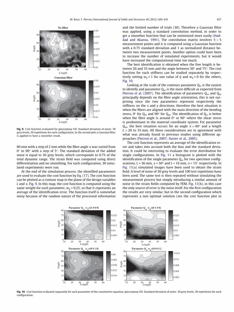
Fig. 9. Cost function evaluated for glass/epoxy UD. Standard deviation of noise: 30grey levels, 30 repetitions for each configuration. In the second plot a Gaussian filteris applied to have a smoother result.

M. Rossi, F. Pierron / International Journal of Solids and Structures 49 (2012) 420–435 427

60 mm with a step of 2 mm while the fibre angle a was varied from0� to 90� with a step of 5�. The standard deviation of the addednoise is equal to 30 grey levels, which corresponds to 0.7% of thetotal dynamic range. The strain field was computed using directdifferentiation and no smoothing. For each configuration, 30 simu-lated experiments were run.

At the end of the simulation process, the identified parametersare used to evaluate the cost function by Eq. (17). The cost functioncan be plotted as a contour map in the plane of the design variablesL and a, Fig. 9. In this map, the cost function is computed using thesame weight for each parameter, wij = 0.25, so that it represents anaverage of the identification error. The function itself is somewhatnoisy because of the random nature of the processed information

Length

Ang

le

Parameter Qxx

wij=[1 0 0 0]

10 20 30 40 50 600

15

30

45

60

75

90

0.005

0.01

0.015

0.02

0.025

Ang

le

Length

Ang

le

Parameter Qxy

wij=[0 0 1 0]

10 20 30 40 50 600

15

30

45

60

75

90

0.016

0.032

0.048

0.064

0.08

Fig. 10. Cost function evaluated separately for each parameter of the constitutive equatioconfiguration.

and the limited number of trials (30). Therefore a Gaussian filterwas applied, using a standard convolution method, in order toget a smoother function that can be minimized more easily (Had-dad and Akansu, 1991). The convolution matrix involves 5 � 5measurement points and it is computed using a Gaussian functionwith a 0.75 standard deviation and 1 as normalized distance be-tween two measurement points. Another option could have beento increase the number of simulated experiments, but it wouldhave increased the computational time too much.

The best identification is obtained when the free length is be-tween 20 and 35 mm and the angle between 50� and 75�. The costfunction for each stiffness can be studied separately by respec-tively setting wij = 1 for one value of ij and wij = 0 for the others,Fig. 10.

Looking at the scale of the contours parameter Qss is the easiestto identify and parameter Qxy is the most difficult as expected fromPierron et al. (2007). The identification of parameters Qxx and Qyy

principally depends on the fibre angle orientation, this is not sur-prising since the two parameters represent respectively thestiffness on the x and y directions, therefore the best situation iswhen the fibres are aligned with the main direction of the bendingstress, 0� for Qxx and 90� for Qyy. The identification of Qss is betterwhen the fibre angle is around 0� or 90� where the shear stressis predominant in the material coordinate system. For parameterQxy, the best situation occurs for an angle a ’ 60� and a lengthL ’ 20 to 35 mm. All these considerations are in agreement withwhat was already found in previous studies using different ap-proaches (Pierron et al., 2007; Xavier et al., 2005).

The cost function represents an average of the identification er-ror and takes into account both the bias and the standard devia-tion. It could be interesting to evaluate the error distribution forsingle configurations. In Fig. 11 a histogram is plotted with theidentification of the single parameter Qxx for two specimen config-urations, L = 36 mm, a = 50� and L = 16 mm, a = 15� respectively. InFig. 11(a) simulated images have been used to obtain the strainfield. A level of noise of 30 grey levels and 100 test repetitions havebeen used. The same test is then repeated without simulating themeasurement process but simply introducing a similar amount ofnoise in the strain fields computed by FEM, Fig. 11(b), in this casethe only source of error is the noise itself. For the first configurationthe results are very similar, but in the second configuration whichrepresents a non optimal solution (see the cost function plot in

Length

Parameter Qyy

wij=[0 1 0 0]

10 20 30 40 50 600

15

30

45

60

75

90

0.005

0.01

0.015

0.02

0.025

Length

Ang

le

Parameter Qss

wij=[0 0 0 1]

10 20 30 40 50 600

15

30

45

60

75

90

0.002

0.005

0.008

0.011

0.014

n, glass/epoxy UD. Standard deviation of noise: 30 grey levels, 30 repetitions for each

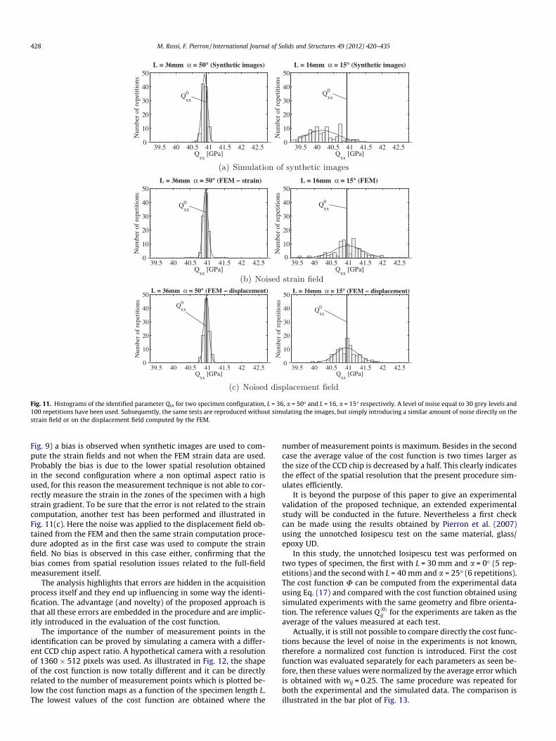
Fig. 11. Histograms of the identified parameter Qxx for two specimen configuration, L = 36, a = 50� and L = 16, a = 15� respectively. A level of noise equal to 30 grey levels and100 repetitions have been used. Subsequently, the same tests are reproduced without simulating the images, but simply introducing a similar amount of noise directly on thestrain field or on the displacement field computed by the FEM.

428 M. Rossi, F. Pierron / International Journal of Solids and Structures 49 (2012) 420–435

Fig. 9) a bias is observed when synthetic images are used to com-pute the strain fields and not when the FEM strain data are used.Probably the bias is due to the lower spatial resolution obtainedin the second configuration where a non optimal aspect ratio isused, for this reason the measurement technique is not able to cor-rectly measure the strain in the zones of the specimen with a highstrain gradient. To be sure that the error is not related to the straincomputation, another test has been performed and illustrated inFig. 11(c). Here the noise was applied to the displacement field ob-tained from the FEM and then the same strain computation proce-dure adopted as in the first case was used to compute the strainfield. No bias is observed in this case either, confirming that thebias comes from spatial resolution issues related to the full-fieldmeasurement itself.

The analysis highlights that errors are hidden in the acquisitionprocess itself and they end up influencing in some way the identi-fication. The advantage (and novelty) of the proposed approach isthat all these errors are embedded in the procedure and are implic-itly introduced in the evaluation of the cost function.

The importance of the number of measurement points in theidentification can be proved by simulating a camera with a differ-ent CCD chip aspect ratio. A hypothetical camera with a resolutionof 1360 � 512 pixels was used. As illustrated in Fig. 12, the shapeof the cost function is now totally different and it can be directlyrelated to the number of measurement points which is plotted be-low the cost function maps as a function of the specimen length L.The lowest values of the cost function are obtained where the

number of measurement points is maximum. Besides in the secondcase the average value of the cost function is two times larger asthe size of the CCD chip is decreased by a half. This clearly indicatesthe effect of the spatial resolution that the present procedure sim-ulates efficiently.

It is beyond the purpose of this paper to give an experimentalvalidation of the proposed technique, an extended experimentalstudy will be conducted in the future. Nevertheless a first checkcan be made using the results obtained by Pierron et al. (2007)using the unnotched Iosipescu test on the same material, glass/epoxy UD.

In this study, the unnotched Iosipescu test was performed ontwo types of specimen, the first with L = 30 mm and a = 0� (5 rep-etitions) and the second with L = 40 mm and a = 25� (6 repetitions).The cost function U can be computed from the experimental datausing Eq. (17) and compared with the cost function obtained usingsimulated experiments with the same geometry and fibre orienta-tion. The reference values Q ð0Þij for the experiments are taken as theaverage of the values measured at each test.

Actually, it is still not possible to compare directly the cost func-tions because the level of noise in the experiments is not known,therefore a normalized cost function is introduced. First the costfunction was evaluated separately for each parameters as seen be-fore, then these values were normalized by the average error whichis obtained with wij = 0.25. The same procedure was repeated forboth the experimental and the simulated data. The comparison isillustrated in the bar plot of Fig. 13.

Fig. 12. Effect of the number of measurement points. The size of the CCD chip changes the shape of the cost function. The lowest values are observed where the number ofmeasurement points is maximum.

M. Rossi, F. Pierron / International Journal of Solids and Structures 49 (2012) 420–435 429

A mismatch is normal because of the low number of repetitionsavailable in the experimental tests. However the simulated proce-dure is able to reproduce qualitatively the trend observed in theexperiments. Parameter Qxx is identified with good accuracy inboth configurations. The identification of Qyy however is much bet-ter in the 25� configuration. Qss has a good identification in bothcases but the 0� configuration gives the best outcome. About Qxy,which is the most difficult parameter to identify, more scatter isexpected, nevertheless the experiments show a better identifica-

Fig. 13. Comparison between simulated and actual experiments from Pierron et al.(2007). The cost function was normalized dividing by the average error, twoconfigurations were evaluated.

tion in the 0� configuration and the same trend is obtained usingthe simulated data.

This is only a first analysis, more experimental tests are needed.However the developed procedure seems to be reliable in compar-ing different configurations.

4.3. Sensitivity to scaling

The scaling procedure introduced in Section 3.2 influences thecost function. The adopted failure criterion is quite simplistic andthe limit stresses listed in Table 1 are generic values for a classof material. In order to have reliable results in the optimization,it is important to verify that the cost function is not stronglydependent on these parameters.

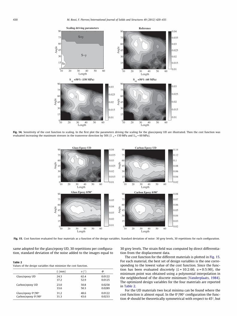
A sensitivity study was conducted on glass/epoxy UD. Accord-ing to the maximum stress criterion, for each configuration, onlyone of the five limit stresses will be involved in the scaling proce-dure, see Eq. (11). The first plot of Fig. 14 shows the parametersdriving the scaling for glass/epoxy UD. This scaling is mainly drivenby the maximum stresses in the transverse direction (S�y and S+y).In order to assess the sensitivity of the proposed procedure to thescaling parameters, the cost function was evaluated using the sametest conditions but increasing the failure stresses S�y and S�y by50%.

The comparison of the cost functions obtained with the in-creased values and the reference one is also illustrated in Fig. 14.The plots look similar, no remarkable changes are produced byincreasing the limit stress. This check suggests that the procedurewill return similar results if the material properties are chosenwithin a reasonably wide range.

4.4. Effect of anisotropy

The cost function described previously can be used to optimizethe test configuration. Indeed the best set of design variables canbe considered as the one that minimizes the cost function. The pur-pose of this section is to study how this choice is influenced by thematerial anisotropy. Four different composite materials were ana-lyzed, the mechanical properties have already been reported in Ta-ble 1.

The cost function was evaluated using the same weight(wij = 0.25) for the four parameters. The test conditions are the

Length

Ang

le

Scaling driving parameters

10 20 30 40 50 600

15

30

45

60

75

90

Ss

S−y

S+y

Length

Ang

le

Reference

10 20 30 40 50 600

15

30

45

60

75

90

0.01

0.015

0.02

0.025

0.03

0.035

0.04

Length

Ang

le

S−y

+50% (150 MPa)

10 20 30 40 50 600

15

30

45

60

75

90

0.01

0.015

0.02

0.025

0.03

Length

Ang

le

S+y

+50% (60 MPa)

10 20 30 40 50 600

15

30

45

60

75

90

0.01

0.015

0.02

0.025

0.03

Fig. 14. Sensitivity of the cost function to scaling. In the first plot the parameters driving the scaling for the glass/epoxy UD are illustrated. Then the cost function wasevaluated increasing the maximum stresses in the transverse direction by 50% (S�y = 150 MPa and S+y = 60 MPa).

Length

Ang

le

Glass Epoxy UD

10 20 30 40 50 600

15

30

45

60

75

90

0.01

0.015

0.02

0.025

0.03

0.035

0.04

Length

Ang

le

Carbon Epoxy UD

10 20 30 40 50 600

15

30

45

60

75

90

0.02

0.04

0.06

0.08

0.1

0.12

0.14

Length

Ang

le

Glass Epoxy 0/90°

10 20 30 40 50 600

15

30

45

60

75

90

0.01

0.02

0.03

0.04

0.05

Length

Ang

le

Carbon Epoxy 0/90°

10 20 30 40 50 600

15

30

45

60

75

90

0.02

0.03

0.04

0.05

0.06

0.07

0.08

Fig. 15. Cost function evaluated for four materials as a function of the design variables. Standard deviation of noise: 30 grey levels, 30 repetitions for each configuration.

430 M. Rossi, F. Pierron / International Journal of Solids and Structures 49 (2012) 420–435

same adopted for the glass/epoxy UD, 30 repetitions per configura-tion, standard deviation of the noise added to the images equal to

Table 2Values of the design variables that minimize the cost function.

L (mm) a (�) U

Glass/epoxy UD 24.3 62.4 0.012237.2 52.9 0.0125

Carbon/epoxy UD 23.0 50.8 0.025833.6 50.3 0.0289

Glass/epoxy 0�/90� 31.2 48.6 0.0122Carbon/epoxy 0�/90� 31.3 43.6 0.0233

30 grey levels. The strain field was computed by direct differentia-tion from the displacement data.

The cost function for the different materials is plotted in Fig. 15.For each material, the best set of design variables is the one corre-sponding to the lowest value of the cost function. Since the func-tion has been evaluated discretely (L = 10:2:60, a = 0:5:90), theminimum point was obtained using a polynomial interpolation inthe neighborhood of the discrete minimum (Vanderplaats, 1984).The optimized design variables for the four materials are reportedin Table 2.

For the UD materials two local minima can be found where thecost function is almost equal. In the 0�/90� configuration the func-tion U should be theoretically symmetrical with respect to 45�, but

Standard deviation: 10 grey levels

−10

−5

0

5

x 10−4 Smoothed field

−10

−5

0

5

x 10−4

Standard deviation: 30 grey levels

−10

−5

0

5

x 10−4 Smoothed field

−10

−5

0

5

x 10−4

Standard deviation: 150 grey levels

−10

−5

0

5

x 10−4 Smoothed field

−10

−5

0

5

x 10−4

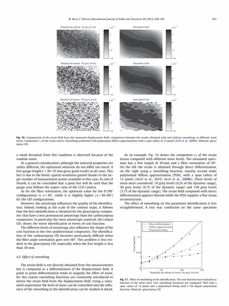
Fig. 16. Computation of the strain field from the measured displacement field: comparison between the results obtained with and without smoothing, at different noiselevels. Component eY of the strain tensor. Smoothing performed with polynomial diffuse approximation with a span radius of 12 pixels (Avril et al., 2008b). Material: glass/epoxy UD.

0 50 100 1500

0.05

0.1

0.15

Standard deviation of noise (in grey levels)

Cos

t fun

ctio

n

Direct differentiationDiffuse approximationPolynomial fitting

Fig. 17. Effect of smoothing in the identification. The cost function was evaluated asfunction of the noise level. Two smoothing functions are compared: PDA with aspan radius of 12 pixels and a polynomial fitting with a 7th degree polynomialfunction. Material: glass/epoxy UD.

M. Rossi, F. Pierron / International Journal of Solids and Structures 49 (2012) 420–435 431

a small deviation from this condition is observed because of therandom noise.

As a general consideration, although the material properties arerather different, the optimized solutions do not differ too much. Afree gauge length L = 30–35 mm gives good results in all cases. Thisfact is due to the better spatial resolution gained thanks to the lar-ger number of measurement points available in this case. As rule ofthumb, it can be concluded that a good test will be such that thegauge area follows the aspect ratio of the CCD camera.

As for the fibre orientation, the optimum value for the 0�/90�configurations is a = 45�, while it is slightly higher (a = 50–60�)for the UD configurations.

However, the anisotropy influences the quality of the identifica-tion. Indeed, looking at the scale of the contour maps, it followsthat the best identification is obtained for the glass/epoxy compos-ites that have a less pronounced anisotropy than the carbon/epoxycomposites. In particular the most anisotropic material, the carbonUD, shows the worst identification in terms of cost function.

The different levels of anisotropy also influence the shape of thecost function in the two unidirectional composites. The identifica-tion of the carbon/epoxy UD becomes particularly difficult whenthe fibre angle orientation goes over 60�. This problem is less evi-dent in the glass/epoxy UD, especially when the free length is lessthan 30 mm.

4.5. Effect of smoothing

The strain field is not directly obtained from the measurementsbut is computed as a differentiation of the displacement field. Apoint to point differentiation tends to magnify the effect of noise,for this reason smoothing functions are commonly introduced toderive the strain field from the displacement field. Using a simu-lated experiment the level of noise can be controlled and the influ-ence of the smoothing in the identification can be studied in detail.

As an example, Fig. 16 shows the component eY of the straintensor computed with different noise levels. The simulated speci-men has a free length of 30 mm and a fibre orientation of 50�.On the left the strain is obtained through direct differentiation,on the right using a smoothing function, namely second orderpolynomial diffuse approximation (PDA), with a span radius of12 pixels (Avril et al., 2010; Avril et al., 2008b). Three levels ofnoise were considered: 10 grey levels (0.2% of the dynamic range),30 grey levels (0.7% of the dynamic range) and 150 grey levels(3.7% of the dynamic range). The strain field computed with directdifferentiation appears blurred while the PDA supplies a fine strainreconstruction.

The effect of smoothing on the parameter identification is lessstraightforward. A test was conducted on the same specimen

432 M. Rossi, F. Pierron / International Journal of Solids and Structures 49 (2012) 420–435

configuration, L = 30 mm and a = 50�, at different levels of noise.For each noise level, the strain was computed using direct differen-tiation, PDA with a span radius of 12 pixels and a global polynomialfitting with a 7th degree polynomial function. The cost functionwas evaluated from the reconstructed strain data and plotted asfunction of the noise level, Fig. 17.

The graph shows that smoothing improves the identificationonly beyond a certain value of noise. In the studied configuration,this noise threshold is around 15 grey level for the PDA and 40 greylevels for the polynomial fitting. After 60 grey levels the polyno-mial fitting returns the best identification. This behaviour can beseen as surprising, since looking at the strain maps of Fig. 16, evenwith a noise standard deviation of 10 grey levels, the strain fieldcomputed with smoothing looks qualitatively much better com-pared to the one computed with direct differentiation.

An explanation can be given on the basis of the VFM theory, seeEq. (8). To identify the parameters, the measured strain compo-nents are multiplied by the virtual strain components, which canbe viewed as weighting functions, and integrated over the surface.The integration gives a first filtering of the strain data. Further-more, using smoothing, the perturbation error due to the noise de-creases but the approximation error increases because thesmoothing acts as a low-pass filter. The balance between thesetwo reconstruction errors makes the smoothing convenient onlyafter a certain noise threshold. The polynomial fitting, that pro-vides strong smoothing of the data, works well for high levels ofnoise but the reconstruction error is larger for small noise level(bias).

This aspect has been studied more deeply using PDA. In fact, thesmoothing capability of PDA can be changed by varying the span

0.

0.

0.

0.

0.

0.

Cos

t fun

ctio

n

5 10 15 200

1

2

3

4

5

6

7

8x 10

−4

Span R [pixel]

Rec

onst

ruct

ion

erro

r

30

60

100150

Fig. 18. Effect of the span R on the strain reconstruction and on the identific

Length

Ang

le

High noise and smoothing

10 20 30 40 50 600

15

30

45

60

75

90

0.02

0.04

0.06

0.08

0.1

Fig. 19. Cost function obtained introducing a high level of noise in the synthetic images (spixels, to compute the strain field. 10 repetitions for each test. Material glass/epoxy UD

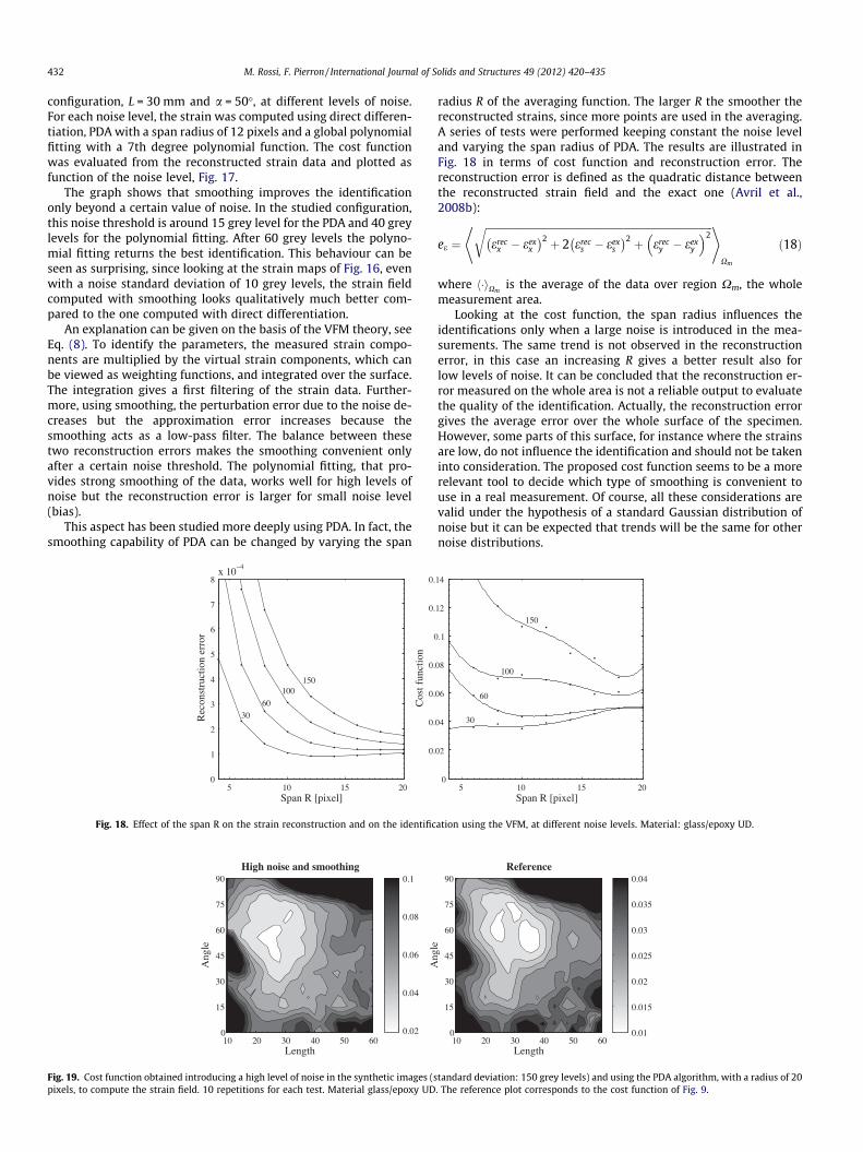
radius R of the averaging function. The larger R the smoother thereconstructed strains, since more points are used in the averaging.A series of tests were performed keeping constant the noise leveland varying the span radius of PDA. The results are illustrated inFig. 18 in terms of cost function and reconstruction error. Thereconstruction error is defined as the quadratic distance betweenthe reconstructed strain field and the exact one (Avril et al.,2008b):

ee ¼ffiffiffiffiffiffiffiffiffiffiffiffiffiffiffiffiffiffiffiffiffiffiffiffiffiffiffiffiffiffiffiffiffiffiffiffiffiffiffiffiffiffiffiffiffiffiffiffiffiffiffiffiffiffiffiffiffiffiffiffiffiffiffiffiffiffiffiffiffiffiffiffiffiffiffiffiffiffiffiffiffiffiffiffiffiffiffiffiffiffierec

x � eexx

� �2 þ 2 erecs � eex

s

� �2 þ erecy � eex

y

� �2r* +

Xm

ð18Þ

where h�iXmis the average of the data over region Xm, the whole

measurement area.Looking at the cost function, the span radius influences the

identifications only when a large noise is introduced in the mea-surements. The same trend is not observed in the reconstructionerror, in this case an increasing R gives a better result also forlow levels of noise. It can be concluded that the reconstruction er-ror measured on the whole area is not a reliable output to evaluatethe quality of the identification. Actually, the reconstruction errorgives the average error over the whole surface of the specimen.However, some parts of this surface, for instance where the strainsare low, do not influence the identification and should not be takeninto consideration. The proposed cost function seems to be a morerelevant tool to decide which type of smoothing is convenient touse in a real measurement. Of course, all these considerations arevalid under the hypothesis of a standard Gaussian distribution ofnoise but it can be expected that trends will be the same for othernoise distributions.

5 10 15 200

02

04

06

08

0.1

12

14

Span R [pixel]

30

60

100

150

ation using the VFM, at different noise levels. Material: glass/epoxy UD.

Length

Ang

le

Reference

10 20 30 40 50 600

15

30

45

60

75

90

0.01

0.015

0.02

0.025

0.03

0.035

0.04

tandard deviation: 150 grey levels) and using the PDA algorithm, with a radius of 20. The reference plot corresponds to the cost function of Fig. 9.

M. Rossi, F. Pierron / International Journal of Solids and Structures 49 (2012) 420–435 433

Another issue is how the smoothing function influences thechoice of the design variables, or, in other words, if the optimizedspecimen configuration obtained for a given material in Section 4.4is still valid when a smoothing function is applied.

The same procedure used to determine the optimal design vari-ables on glass/epoxy UD was repeated using an increased level ofnoise (standard deviation: 150 grey levels) and PDA to computethe strains, with a large span radius of 20 pixel. Only 10 repetitionswere used at each configuration because of the long time requiredby the PDA algorithm. The results are presented in Fig. 19, the ref-erence plot is the cost function evaluated for the same material inFig. 9. Qualitatively, the two cost functions look similar. In this casea minimum was found for L = 29.8 mm and a = 57.5�, not too farfrom the values obtained previously and listed in Table 2. Clearly,looking at the contour scales in the two cases, the average identi-fication error is higher when more noise is introduced. In orderto prove the effectiveness of the PDA in reconstructing the strainfield it can be highlighted that, although the standard deviationof the noise was increased five times, from 30 to 150 grey levels,the average error in the identification increases only by a factorof around two.

On the basis of these results, it seems reasonable to concludethat an optimized configuration found using a low level of noiseand no smoothing will be effective also when a high level of noiseis encountered. From a practical point of view, the possibility ofexcluding the smoothing process in the optimization algorithm,where the cost functions have to be evaluated many times, allowsto save a lot of computational time.

4.6. Influence of missing data

During a real test it is always difficult to measure the displace-ment at the free edges of the specimen and some data are

10 20 30 40 500.02

0.03

0.04

0.05

0.06

0.07

0.08

Number of lost pixels

Cos

t fun

ctio

n

Fig. 20. Identification error as a function of the pixels which are removed from theedges of the specimen.

Length

Missing data

10 20 30 40 50 600

15

30

45

60

75

90

0.02

0.03

0.04

0.05

0.06

0.07

0.08

Ang

le

Ang

le

Fig. 21. Cost function with five rows of measurement points missing at each edge, matecorresponds to the cost function of Fig. 9.

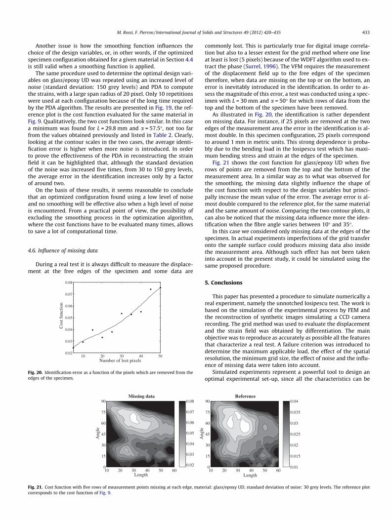
commonly lost. This is particularly true for digital image correla-tion but also to a lesser extent for the grid method where one lineat least is lost (5 pixels) because of the WDFT algorithm used to ex-tract the phase (Surrel, 1996). The VFM requires the measurementof the displacement field up to the free edges of the specimentherefore, when data are missing on the top or on the bottom, anerror is inevitably introduced in the identification. In order to as-sess the magnitude of this error, a test was conducted using a spec-imen with L = 30 mm and a = 50� for which rows of data from thetop and the bottom of the specimen have been removed.

As illustrated in Fig. 20, the identification is rather dependenton missing data. For instance, if 25 pixels are removed at the twoedges of the measurement area the error in the identification is al-most double. In this specimen configuration, 25 pixels correspondto around 1 mm in metric units. This strong dependence is proba-bly due to the bending load in the Iosipescu test which has maxi-mum bending stress and strain at the edges of the specimen.

Fig. 21 shows the cost function for glass/epoxy UD when fiverows of points are removed from the top and the bottom of themeasurement area. In a similar way as to what was observed forthe smoothing, the missing data slightly influence the shape ofthe cost function with respect to the design variables but princi-pally increase the mean value of the error. The average error is al-most double compared to the reference plot, for the same materialand the same amount of noise. Comparing the two contour plots, itcan also be noticed that the missing data influence more the iden-tification when the fibre angle varies between 10� and 35�.

In this case we considered only missing data at the edges of thespecimen. In actual experiments imperfections of the grid transferonto the sample surface could produces missing data also insidethe measurement area. Although such effect has not been takeninto account in the present study, it could be simulated using thesame proposed procedure.

5. Conclusions

This paper has presented a procedure to simulate numerically areal experiment, namely the unnotched Iosipescu test. The work isbased on the simulation of the experimental process by FEM andthe reconstruction of synthetic images simulating a CCD camerarecording. The grid method was used to evaluate the displacementand the strain field was obtained by differentiation. The mainobjective was to reproduce as accurately as possible all the featuresthat characterize a real test. A failure criterion was introduced todetermine the maximum applicable load, the effect of the spatialresolution, the minimum grid size, the effect of noise and the influ-ence of missing data were taken into account.

Simulated experiments represent a powerful tool to design anoptimal experimental set-up, since all the characteristics can be

Length

Reference

10 20 30 40 50 600

15

30

45

60

75

90

0.01

0.015

0.02

0.025

0.03

0.035

0.04

rial: glass/epoxy UD, standard deviation of noise: 30 grey levels. The reference plot

434 M. Rossi, F. Pierron / International Journal of Solids and Structures 49 (2012) 420–435

easily varied. In the present case they were used to optimize thefree length and the fibre angle of the specimen for four compositematerials. The VFM was used to identify the constitutive parame-ters and a cost function was introduced to evaluate the error andfind the best set of design variables.

The obtained results appear reasonable and in line with theexperiments conducted on similar materials with the Iosipescutest. This gives a first confirmation of the effectiveness of theadopted procedure.

The main outcomes from the present study are as follows.

� It has been demonstrated that it is possible to numericallysimulate, in a realistic way, an experimental test which usesfull-field measurements to identify the material properties ofcomposites. Simulated experiments represent a useful tool toimprove the design of actual tests.� The spatial resolution of the measurement technique plays an

important role in the parameter identification. In designingexperiments, it is advisable to use specimen shapes thatapproach the aspect ratio of the CCD chip.� A high anisotropy has a detrimental influence on the identifica-

tion in terms of global error, however it influences less theshape of the cost function and the choice of the optimal designvariables. As a consequence, the same test configuration can beefficiently used to test different types of composites.� The necessity of introducing smoothing in the identification

depends on the amount of noise. For a given specimen configu-ration, smoothing becomes necessary beyond a certain noisethreshold which can be evaluated with the proposed procedure.� Using the unnotched Iosipescu test and the VFM, the data mea-

sured close to the edges of the specimen bear a great impor-tance in the parameter identification. A measurementtechnique that allows to reduce the missing data at the edgeswill considerably improve the reliability of the identification.

In the future, the idea is to use the present procedure to designautomatically more complex specimen shapes, that, for example,will be less sensitive to the missing data at the edges. Other full-field techniques, for instance digital image correlation, can beintroduced in the procedure. Finally, to have a definitive check ofthe effectiveness of the developed procedure, a thorough experi-mental study is needed to validate the numerical optimization.

References

Avril, S., Ferrier, E., Hamelin, P., Surrel, Y., Vautrin, A., 2004a. A full-field opticalmethod for the experimental analysis of reinforced concrete beams repairedwith composites. Compos. Part A – Appl. S. 35, 873–884.

Avril, S., Grédiac, M., Pierron, F., 2004b. Sensitivity of the virtual fields method tonoisy data. Comput. Mech. 34 (6), 439–452.

Avril, S., Vautrin, A., Surrel, Y., 2004c. Grid method: application to thecharacterization of cracks. Exp. Mech. 44 (1), 37–43.

Avril, S., Bonnet, M., Bretelle, A.-S., Grédiac, M., Hild, F., Ienny, P., Latourte, F.,Lemosse, D., Pagano, S., Pagnacco, E., Pierron, F., 2008a. Overview ofidentification methods of mechanical parameters based on full-fieldmeasurements. Exp. Mech. 48, 381–402.

Avril, S., Feissel, P., Pierron, F., Villon, P., 2008b. Estimation of the strain field fromfull-field displacement noisy data. Rev. Eur. Méc Numér. 17 (5–7), 857–868.

Avril, S., Feissel, P., Pierron, F., Villon, P., 2010. Comparison of two approaches fordifferentiating full-field data in solid mechanics. Meas. Sci. Technol. 21 (1),015703, 11 p.

Bornert, M., Brémand, F., Doumalin, P., Dupré, J.-C., Fazzini, M., Grédiac, M., Hild, F.,Mistou, S., Molimard, J., Orteu, J.-J., Robert, L., Surrel, Y., Vacher, P., Wattrisse, B.,2009. Assessment of digital image correlation measurement errors:methodology and results. Exp. Mech. 49, 353–370.

Bui, H.D., Constantinescu, A., Maigre, H., 2004. Numerical identification of linearcracks in 2d elastodynamics using the instantaneous reciprocity gap. InverseProblems 20, 993–1001.

Chalal, H., Avril, S., Pierron, F., Meraghni, F., 2006. Experimental identification of anonlinear model for composites using the grid technique coupled to the virtualfields method. Compos. Part A – Appl. S. 37 (2), 315–325.

Claire, D., Hild, F., Roux, S., 2004. A finite element formulation to identify damagefields: the equilibrium gap method. Int. J. Numer. Methods Eng. 61, 189–208.

Cooreman, S., Lecompte, D., Sol, H., Vantomme, J., Debruyne, D., 2008. Identificationof mechanical material behavior through inverse modeling and DIC. Exp. Mech.48 (4), 421–433.

Geymonat, G., Pagano, S., 2003. Identification of mechanical properties bydisplacement field measurement: a variational approach. Meccanica 38, 535–545.

Giraudeau, A., Pierron, F., 2005. Identification of stiffness and damping properties ofthin isotropic vibrating plates using the virtual fields method. Theory andsimulations. J. Sound Vib. 284, 757–781.

Grédiac, M., 2004. The use of full-field measurement methods in composite materialcharacterization: interest and limitations. Compos. Part A – Appl. S. 35, 751–761.

Grédiac, M., Pierron, F., 2006. Applying the virtual fields method to theidentification of elasto-plastic constitutive parameters. Int. J. Plasticity 22,602–627.

Grédiac, M., Vautrin, A., 1990. A new method for determination of bending rigiditiesof thin anisotropic plates. J. Appl. Mech. 57, 964–968.

Grédiac, M., Toussaint, E., Pierron, F., 2002a. Special virtual fields for the directdetermination of material parameters with the virtual fields method. Part 1:Principle and definition. Int. J. Solids Struct. 39, 2691–2705.

Grédiac, M., Toussaint, E., Pierron, F., 2002b. Special virtual fields for the directdetermination of material parameters with the virtual fields method. Part 2:Application to in-plane properties. Int. J. Solids Struct. 39, 2707–2730.

Grédiac, M., Pierron, F., Avril, S., Toussaint, E., 2006. The virtual fields method forextracting constitutive parameters from full-field measurements: a review.Strain 42, 233–253.

Haddad, R., Akansu, A., 1991. A class of fast Gaussian binomial filters for speech andimage processing. IEEE Trans. Signal. Process. 39, 723–727.

Kajberg, J., Lindkvist, G., 2004. Characterisation of materials subjected to largestrains by inverse modelling based on in-plane displacement fields. Int. J. SolidsStruct. 41, 3439–3459.

Latourte, F., Chrysochoos, A., Pagano, S., Wattrisse, B., 2008. Elastoplastic behavioridentification for heterogeneous loadings and materials. Exp. Mech. 48 (4), 435–449.

Lecompte, D., Smits, A., Sol, H., Vantomme, J., Van Hemelrijck, D., 2007. Mixednumerical–experimental technique for orthotropic parameter identificationusing biaxial tensile tests on cruciform specimens. Int. J. Solids Struct. 44 (5),1643–1656.

Le Magorou, L., Bos, F., Rouger, F., 2002. Identification of constitutive laws for wood-based panels by means of an inverse method. Compos. Sci. Technol. 62, 591–596.

Meuwissen, M.H.H., Oomens, C.W.J., Baaijens, F.P.T., Petterson, R., Janssen, J.D.,1998. Determination of the elasto-plastic properties of aluminium using amixed numerical–experimental method. J. Mater. Process. Technol. 75, 204–211.

Moulart, R., Avril, S., Pierron, F., 2006. Identification of the through-thicknessrigidities of a thick laminated composite tube. Compos. Part A – Appl. S. 37,326–336.

Moulart, R., Rotinat, R., Pierron, F., Lerondel, G., 2007. On the realization ofmicroscopic grids for local strain measurement by direct interferometricphotolithography. Opt. Laser Eng. 45 (12), 1131–1147.

Moulart, R., Rotinat, R., Pierron, F., 2009. Full-field evaluation of the onset ofmicroplasticity in a steel specimen. Mech. Mater. 41 (11), 1207–1222.

Orteu, J.-J., Garcia, D., Robert, L., Bugarin, F., 2006. A speckle-texture imagegenerator. In: Proceedings of the Speckle’06 Onternational Conference, Nîmes,France.

Pierron, F. 1994. New Iosipescu fixture for the measurement of the in-plane shearmodulus of laminated composites: design and experimental procedure.Technical Report 940125, Ecole des Mines de Saint-Etienne.

Pierron, F., 1998. Saint-Venant effects in the Iosipescu specimen. J. Compos. Mater.32 (22), 1986–2015.

Pierron, F., Grédiac, M., 2000. Identification of the through-thickness moduli of thickcomposites from whole-field measurements using the Iosipescu fixture: theoryand simulations. Compos. Part A – Appl. S. 31, 309–318.

Pierron, F., Vert, G., Burguete, R., Avril, S., Rotinat, R., Wisnom, M., 2007.Identification of the orthotropic elastic stiffnesses of composites with thevirtual fields method: sensitivity study and experimental validation. Strain 43(3), 250–259.

Piro, J.-L., Grédiac, M., 2004. Producing and transferring low-spatial-frequency gridsfo measuring displacement fields with moiré and grid methods. Exp. Tech. 28,23–26.

Rossi, M., Broggiato, G.B., Papalini, S., 2008. Application of digital image correlationto the study of planar anisotropy of sheet metals at large strains. Meccanica 43(2), 185–199.

Soden, P.D., Hinton, M.J., Kaddour, A.S., 1998. Comparison of the predictivecapabilities of current failure theories for composite laminates. Compos. Sci.Technol. 58, 1225–1254.

Soden, P.D., Kaddour, A.S., Hinton, M.J., 2004. Recommendations for designers andresearchers resulting from the world-wide failure exercise. Compos. Sci.Technol. 64, 589–604.

Surrel, Y., 1994. Moiré and grid methods: a signal-processing approach. In:Interferometry ’94: Photomechanics, SPIE, vol. 2342.

Surrel, Y., 1996. Design of algorithms for phase measurements by the use of phase-stepping. Appl. Opt. 35, 51–60.

M. Rossi, F. Pierron / International Journal of Solids and Structures 49 (2012) 420–435 435

Surrel, Y., 1997. Design of phase-detection algorithms insensitive to biasmodulation. Appl. Opt. 36, 805–807.

Surrel, Y., 1999. Photomecanics. Springer, Berlin (Chapter Fringe analysis) pp. 57–104.

Syed-Muhammad, K., Toussaint, E., Grédiac, M., Avril, S., Kim, J., 2009.Characterization of composite plates using the virtual fields method withoptimized loading conditions. Compos. Struct. 85, 70–82.

Tsai, H.W., Hahn, H.T., 1980. Introduction to Composite Materials. TechonomicPublishing Company, Inc.

Vanderplaats, G.N., 1984. Numerical Optimization Techniques for EngineeringDesign: with Applications. McGraw-Hill, New York (Chapter 2).

Xavier, J., Avril, S., Pierron, F., Morais, J., Marinescu, M., 2005. Identification of clearwood orthotropic stiffness using full-field measurements. In: European

Mechanics of Materials Conference (EMMC8): Material and StructuralIdentification from Full-field Measurements, 13–15 September, Cachan,France.

Xavier, J., Avril, S., Pierron, F., Morais, J., 2007. Novel experimental approach for thecharacterisation of the LR stiffnesses of clear wood using a single specimen.Holzforschung 61, 573–581.

Zinoviev, P., Grigoriev, S.V., Lebedeva, O.V., Tairova, L.R., 1998. Strength ofmultilayered composites under plane stress state. Compos. Sci. Technol. 58,1107–1124.

Zinoviev, P.A., Lebedeva, O.V., Tairova, L.P., 2002. Coupled analysis of experimentaland theoretical results on the deformation and failure of laminatedcomposites under a plane state of stress. Compos. Sci. Technol. 62, 11711–11724.