On the Performance and Use of Government Revenue Forecasts

Alan J. AuerbachUniversity of California, Berkeley and NBER

July 20, 1999

This paper has been written to appear as the National Tax Journal’s Beck Memorial Paper. I amgrateful to Jonathan Siegel for assistance and to him, Richard Blundell, Mark Booth, DougHoltz-Eakin, and participants in a seminar at the American Enterprise Institute for suggestionsand comments on earlier drafts. I also thank Mary Barth of OMB and Geoff Lubien of DRI forproviding forecast data from their respective organizations, and the Burch Center for Tax Policyand Public Finance for financial support. Any views expressed are my own, and not necessarilythose of any organization with which I am affiliated.

Introduction

Over the years, a key issue in the design of fiscal policy rules has been the accuracy of

government budget forecasts, particularly those of tax revenues. During the early years of the

Reagan administration, “supply-side” forecasts of budget surpluses gave way to the reality of

large deficits that persisted into the 1990s, despite several policy changes aimed at deficit

reduction (Auerbach 1994). The persistence of overly optimistic forecasts led to the perception

that, as budget forecasts came to occupy a more central role in the policy process, the pressure on

forecasters to help policy makers avoid hard choices led to forecasting bias. However, the

experience of recent years suggests that prior conclusions may need to be amended.

The remarkable U.S. economic expansion of the 1990s has also been a challenging period

for government revenue forecasters, but with different consequences than before. Continual

surprises as to the overall strength of the U.S. economy and the share of income going to those in

the top income tax brackets have led to a series of what turned out to be overly pessimistic

aggregate revenue forecasts. Large predicted deficits gave way to smaller predicted deficits and,

ultimately, the realization of budget surpluses and the forecast of larger surpluses to come.

These large revisions have had a significant impact on the budget process of a government that

has lashed itself to the mast of revenue forecasts to help it withstand the political sirens in its

path. Even without such budget rules, though, revenue forecasts would remain an important

input to the design of fiscal policy, for they provide a sense of what fiscal actions are sustainable

over the longer term.

Some critics of the recent government revenue forecasts have suggested a bias, albeit in

the direction opposite to that argued to exist in the earlier period. They point to the size of

forecast errors and the consistent sign of these errors in arguing that the forecasters should have

2

been able to do better. But over short periods, any sequence of individual forecast errors can be

given a rational justification, and virtually any statistical error pattern is consistent with an

efficient forecasting process that uses all available information in forming its predictions. One

needs more data to get a better sense of whether the recent forecasts really are consistent with

forecast efficiency, or whether they simply illustrate the continuation of a process of biased

forecasting, with perhaps a change in bias.

In this paper, I begin by considering the issue of forecast bias and efficiency. To do so, I

augment the recent data in three ways. First, I consider forecasts over a longer period. Second, I

compare these government revenue forecasts to contemporaneous private forecasts. Finally, I

distinguish forecasting errors according to their source, to get a better idea of the extent to which

what are called “errors” are attributable to institutional forecasting conventions. After

performing this data analysis, I go on to consider its implications for the forecasting process, and

the use to which revenue forecasts should be put.

The results of analyzing the data are mixed. On the one hand, the performance of

government forecasters – the Congressional Budget Office (CBO) and the Office of Management

and Budget (OMB) – has not differed significantly from that of the private forecaster, Data

Resources, Inc., (DRI). Further, over the full period considered, there is no evidence that either

OMB or CBO has been overly pessimistic in its revenue forecasts. The recent string of overly

pessimistic forecasts is balanced by an even more impressive string of overly optimistic forecasts

in the years immediately preceding the current expansion. Even when the “pessimistic” and

“optimistic” periods are considered separately, forecast errors have such large standard errors

that it is difficult to conclude that the forecasts exhibit any underlying bias.

3

On the other hand, I also find that the government forecasts fail various statistical tests of

efficiency; in principle, the process could be improved. In particular, the forecast revisions

exhibit significant serial correlation and, perhaps more puzzling, the patterns of bias in revisions

exhibit strong seasonality.

These results suggest that government revenue forecasts could convey more information

than they do at present. But without understanding the reasons for existing forecast inefficiency,

it is not clear how to accomplish this objective. Further, the large standard errors associated with

the forecasts remind us of the care needed in the use of point estimates for policy purposes.

Because the budget process ignores the uncertainty inherent in individual forecasts, the “best”

forecasts for budget purposes need not be the most accurate point estimates; it might well be

appropriate, for example, for these forecasts to reflect a pessimistic bias. In short, the

requirements of forecast efficiency and those of a poorly conceived budget process are

inconsistent. Perhaps both needs would be best served simultaneously through a separation of

forecasting into “official” and “unofficial” functions, although it is unclear how such functions

can be kept distinct.

Data and Methodology

Twice each year (and, on occasion, more frequently), CBO and OMB produce revenue

forecasts for the current and several upcoming fiscal years. One forecast typically occurs around

the beginning of February with the presentation of the Federal Budget by OMB and the roughly

coincident Economic and Budget Outlook published by CBO. The second typically occurs in

August or September, with OMB’s Midsession Review and CBO’s Economic and Budget

4

Outlook: An Update. For most of the sample period, both winter and summer forecasts have

been for six fiscal years, including the one ending September 30 of the same year.1

In revising its revenue forecasts for a particular year, each government agency

incorporates changes in its own economic forecasts as well as estimates of the effects of policy

changes. For a number of years, both CBO and OMB have followed the practice of dividing

each forecast revision into three mutually exclusive categories: policy, economic, and technical.

Policy revisions are those attributed to changes from “baseline” policy. Economic revisions are

changes attributed to macroeconomic events. Technical revisions are residual, containing

changes that the agency attributes neither to policy nor to macroeconomic changes. For

example, a technical revision in revenue would result from a change in the rate of tax evasion, a

shift in the composition of capital income from dividends to capital gains, or a change in the

distribution of income.

We may express this revision process as:

(1) xi,t - xi+1,t-1 = pi,t + ei,t + ri,t

where xi,t is the i-step-ahead forecast at date t and pi,t, ei,t, and ri,t are the policy, economic, and

technical components of the revision in this forecast from period t-1. For CBO, these

semiannual data on revisions are available continuously from 1984 through the present. While

OMB does not publish comparable forecasts, it has produced them internally for revenues over

roughly the same period, for the same forecast horizons as are considered by CBO. For the two

agencies together, comparable semiannual data are continuously available for revisions during

1 Recently, CBO has begun to report forecasts over an eleven-year horizon.

5

the period from the summer of 1985 to the winter of 1999.2 Initially, I analyze the sample that

beings one forecasting period later, with the revision between forecasts made in the summer of

1985 and the winter of 1986, for this is the first period for which I have been able to obtain

comparable DRI forecasts.3 For the corresponding DRI forecasts, though, only the aggregate

revisions, xi,t - xi+1,t-1, are available.

Because there are two forecasts made each year for revenues in each of six fiscal years,

there are twelve forecast horizons and twelve corresponding revisions for the revenues of each

fiscal year being predicted. The last such revision, however, differs from the others, in that it

reflects changes over the very brief period between the late summer forecast during the fiscal

year itself and the September 30 end of that fiscal year.4 Thus, for the statistical analysis below,

I consider only the first eleven forecast revisions for each fiscal year, labeling these revisions 1

(shortest horizon, from winter to summer during the fiscal year itself) through 11 (longest

horizon, five years earlier). Odd-numbered revisions are those occurring between winter and

summer; even-numbered revisions are those occurring between summer and winter. I refer to

the final revision, occurring between the final forecast and the end of the fiscal year, as revision

0.

Figure 1 illustrates the timing of revisions made by OMB during the last full fiscal year in

the sample, 1998, showing the correspondence between revision horizons and fiscal years. For

2 Actually, OMB and CBO data on overall revisions xi,t - xi+1,t-1 – but not their breakdown by source – may beconstructed for a longer period from successive revenue forecasts, xi,t. For an analysis of revisions during this earlierperiod, see Plesko (1988).3 DRI makes forecasts at 3-year horizons monthly, but publishes long-range (10-year) forecasts only twice a year –currently in May and November, but with some timing changes over the years. For purposes of comparison with theforecasts of CBO and OMB, I align the May and November forecasts with the CBO and OMB forecastsimmediately following.4 Indeed, CBO does not provide a breakdown of this last forecast revision into components.

6

example, the revision at horizon 5 included in the 1998 Midsession Review was the change in

forecast revenue for fiscal year 2000 from that given one period earlier, in winter 1998.

Revision Patterns

Table 1 presents basic means for OMB, CBO and DRI forecast revisions, for the period

1986-99. To ensure that revisions from different years comparable, each revision is scaled by a

projected value of the revenue being forecast, based on an exponential time trend, and expressed

as a percentage of trend revenue (i.e., multiplied by 100). The mean cumulative revision equals

the sum of the means at each horizon; it represents an estimate of the cumulative revision (as a

percentage of trend revenues) during the period from initial to final published forecast for a

particular fiscal year’s revenue.5

A basic implication of the theory of optimal forecast behavior is that forecasts should

have no systematic bias, at least if the perceived costs of forecast errors are symmetric. Over a

long enough period, then, the mean forecast errors should not differ significantly from zero.

Looking at the means in Table 1, then, the most notable aspect of these individual and

cumulative averages is that they are reasonably close to zero; they do not reveal the huge upward

revisions of recent years. Indeed, the OMB and DRI averages indicate net downward revenue

revisions, the CBO net is only slightly positive, and all three sets of cumulative revisions average

less than 1.5 percent of revenue in absolute value over the six-year revision period – hardly an

enormous error.

5 Note that this is not equal to the average cumulative error during the period for fiscal years for which completeforecast data are available, for it also incorporates the long-horizon revisions for future fiscal years and short-horizon revisions for fiscal years early in the sample.

7

However, if one breaks the sample down into periods of roughly equal length defined by

the election of Bill Clinton in 19926, as is done in Table 2, it is evident that the aggregate results

mask very different experience during the two distinct periods. All three organizations have

revised their forecasts sharply upward during this period, with CBO’s revisions being greatest

and OMB’s smallest.

This sharp break in forecast patterns coincident with a change in the political landscape is

suggestive. Persistent errors in one direction could be produced by a bias in favor of initial

overstatement or understatement of expected revenues. Hence, the observed pattern is consistent

with a shift in bias from one favoring overstatement (and hence eventually having to revise

revenue forecasts downward) to a bias toward understatement (and eventually having to revise

revenue forecasts upward). Indeed, this is a plausible scenario, given the change in climate in

1993, as exemplified by the enactment of a large tax increase. However, any explanation based

on government agency bias must confront the fact that the same general pattern of revisions is

observed in the forecasts of a private business that, presumably, is not directly influenced by the

political incentives and pressures that may color the forecasts of those in government.

Even if is not the result of any direct bias, DRI’s relative performance does not, in itself,

rule out the possibility of government agency bias. A bias could spread indirectly if private

forecasters had little independent information and there were strong enough incentives not to

deviate too much from “consensus” estimates. Such behavior could be justified more formally

using models in which a principal must set an agent’s compensation and cannot fully identify

6 This procedure includes the winter, 1993 revisions in the pre-Clinton period. This set of revisions was the first touse forecasts made by the Clinton administration. Hence, the revisions span the presidential transition. It is notclear how these revisions should be treated, if one wishes to distinguish behavior in the two periods. However,leaving this observation period out or including it in the Clinton period does not have an important impact on theresults presented.

8

the sources of particular errors. Considering relative performance helps distinguish between

errors caused by common shocks and those caused by the agent’s own limitations (e.g.,

Holmstr m 1982), but it may, in turn, lead to an incentive to follow the behavior of others

(Scharfstein and Stein, 1990; Zweibel 1995). The impact of this incentive has been considered

(and some of its cross-section implications rejected, notably that forecasters would tend to mimic

the predictions of forecasters deemed most competent) in a related context by Ehrbeck and

Waldmann (1996), who modeled the behavior of professional forecasters predicting Treasury bill

rates.

Indeed, the DRI forecast revisions are strongly correlated with those of CBO and OMB.

While the CBO and OMB revisions have a correlation coefficient of .63, the correlations

between DRI and the two agencies are .54 (CBO) and .39 (OMB), values made all the more

remarkable by the fact that the timing of the DRI forecasts differs from those of OMB and CBO.

However, with so little data and so few forecasters, it is not really possible to tell whether this

strength of correlation reflects excessive reliance on government projections, or simply the lack

of independent information. After all, it is not clear how important it is for a private forecaster to

obtain information and make accurate forecasts about government revenues. While clients may

see a direct financial gain from having superior information about the movement of interest rates,

there is no organized market directly tied to the level of government revenues.

Yet another possible explanation for the observed pattern of government forecast

revisions is that the aggregate forecasts considered thus far do not really represent statistical

predictions of future revenues, but rather “baseline” projections that incorporate assumptions

about future policy that are inconsistent with optimal forecasting procedures. By practice,

baseline forecasts of policy are in some cases determined by certain mechanical rules that do not

9

reflect expectations regarding future policy. As a consequence, many of the revisions attributed

to policy changes do not represent “surprises,” but simply the application of these rules.

Therefore, if one wishes to determine the extent to which forecasts reflect the unbiased and

efficient use of available information, it is useful to exclude policy revisions from the analysis.

One might further divide the remaining revisions into their “economic” and “technical”

components, making it possible, potentially, to determine the extent to which forecasting errors

arise from underlying macroeconomic forecasts, as opposed to other factors. This would be a

useful exercise, as the macroeconomic forecasts and the ultimate revenue projections are

typically done in stages by separate groups of individuals. However, the distinction between

these two components is somewhat arbitrary. For example, the impact of revisions to the

macroeconomic forecast that are anticipated but not yet “official” at the time of a revenue

forecast may be incorporated as a “technical” element.

Some initial analysis suggests that the components do not represent “independent”

sources of error, and that OMB and CBO use different methodologies to divide forecast revisions

into these two categories.7 Thus, I focus only on these two components together for each

agency, represented by the sum ei,t + ri,t in expression (1). For compactness of notation, I refer to

this sum as yi,t. Unfortunately, the same exercise cannot be conducted for the DRI forecasts,

revisions of which are not broken down by category.

7 Particularly for OMB, the technical and economic revisions are not independent. At all but the longest horizon, theOMB technical and economic forecast revisions are negatively correlated. Also, while technical and economicrevisions are both highly correlated at contemporaneous horizons across agencies (with coefficients of .73 and .64,respectively), the combined sums of economic and technical revisions are even more highly correlated (.77). Bycontrast, the policy revisions have a correlation coefficient of only .22, suggesting stronger differences inprocedures.

10

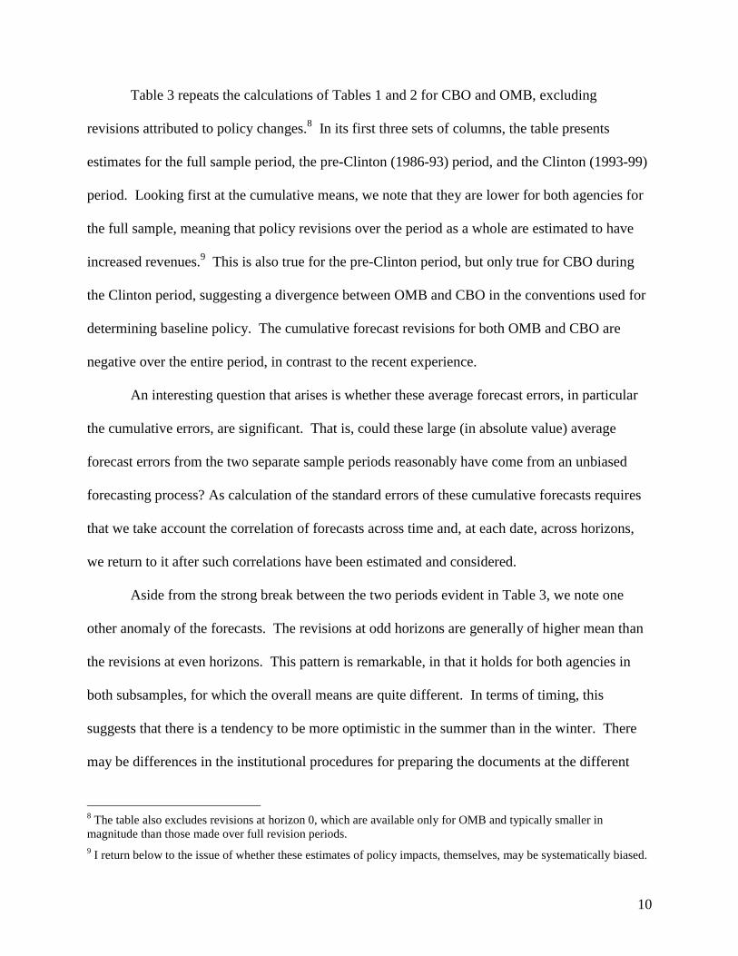
Table 3 repeats the calculations of Tables 1 and 2 for CBO and OMB, excluding

revisions attributed to policy changes.8 In its first three sets of columns, the table presents

estimates for the full sample period, the pre-Clinton (1986-93) period, and the Clinton (1993-99)

period. Looking first at the cumulative means, we note that they are lower for both agencies for

the full sample, meaning that policy revisions over the period as a whole are estimated to have

increased revenues.9 This is also true for the pre-Clinton period, but only true for CBO during

the Clinton period, suggesting a divergence between OMB and CBO in the conventions used for

determining baseline policy. The cumulative forecast revisions for both OMB and CBO are

negative over the entire period, in contrast to the recent experience.

An interesting question that arises is whether these average forecast errors, in particular

the cumulative errors, are significant. That is, could these large (in absolute value) average

forecast errors from the two separate sample periods reasonably have come from an unbiased

forecasting process? As calculation of the standard errors of these cumulative forecasts requires

that we take account the correlation of forecasts across time and, at each date, across horizons,

we return to it after such correlations have been estimated and considered.

Aside from the strong break between the two periods evident in Table 3, we note one

other anomaly of the forecasts. The revisions at odd horizons are generally of higher mean than

the revisions at even horizons. This pattern is remarkable, in that it holds for both agencies in

both subsamples, for which the overall means are quite different. In terms of timing, this

suggests that there is a tendency to be more optimistic in the summer than in the winter. There

may be differences in the institutional procedures for preparing the documents at the different

8 The table also excludes revisions at horizon 0, which are available only for OMB and typically smaller inmagnitude than those made over full revision periods.9 I return below to the issue of whether these estimates of policy impacts, themselves, may be systematically biased.

11

times of the year, but there is not any obvious reason for more bias toward pessimism in the

winter, at the time of initial budget presentation. Indeed, one might have expected the opposite

result, that the pressure toward optimism would be stronger for those initial forecasts given more

attention and hence carrying greater political weight.

Some further insight into this pattern comes from breaking the pre-Clinton period down

even further. The first part of this period, ending with the summer, 1990 revision, corresponds

roughly the era under which the Gramm-Rudman-Hollings (GRH) budget rules were in force –

an era that ended with fall, 1990 “budget summit.” The GRH legislation, first passed in 1985

and later amended, set a deficit target trajectory and required that each year’s budget, as

submitted by the president, conform to that year’s GRH target. Subsequently, during the actual

fiscal year itself, based on the estimate contained in the Midsession Review, GRH could trigger a

sequestration process of automatic budget cuts to meet the budget target. In terms of our

notation, these two aspects of GRH would lead to greater pressure for optimistic forecasts at

horizon 4 (to satisfy the GRH requirement with the initial budget presentation) and horizon 1 (to

avoid sequestration with the current fiscal year’s Midsession Review). It is less clear what this

implies for the forecast revisions, except perhaps that the revisions at horizon 4 should have been

relatively more optimistic.

The last two columns of Table 3 present mean economic and technical revisions for the

GRH period for both OMB and CBO. The revision pattern was different for OMB during the

GRH period. In fact, the shift in seasonal pattern is observable not just around horizon 4, but at

all other horizons as well, with the even horizons now exhibiting more “optimism;” perhaps the

greater optimism of budget-year forecasts spilled over into the other forecasts being made

simultaneously. For such a short sample period, though, it is difficult to know whether this shift

12

was attributable to GRH or to something else. After all, mean revisions during the GRH period

were also much less negative than those from the remainder of the pre-Clinton era, which

covered the 1990-91 recession and the period of relatively slow growth that immediately

followed. Indeed, the onset of that recession contributed to the demise of GRH, as deficit targets

became unachievable. But it is interesting that this seasonal shift is not present in the parallel

forecast revisions of CBO, which was not directly affected by the GRH legislation.

Forecast Evaluation

Using the individual revisions underlying the means in Table 3, one can construct formal

tests of forecast efficiency. Consider the relationship between successive forecast revisions for

the same fiscal year, yi,t and yi+1,t-1. According to theory, if each forecast is unbiased and uses all

information available at the time, these revisions should have a zero mean and should be

uncorrelated. Letting ai be the mean forecast revision for horizon i, we relate these successive

forecasts by the equation:

(2) yi,t – ai = ρi (yi+1,t-1 - ai+1) + εi,t

or

(3) yi,t = ρi yi+1,t-1 + αi + εi,t

where αi = ai – ρi ai+1 and εi,t has zero mean and is serially independent.10 The hypothesis of

forecast efficiency implies that αi = 0 (no bias) and ρi = 0 (no serial correlation).

10 For revisions at horizon 11, there is no lagged revision, so expressions (2) and (3) become y11,t = a11+ε11,t =α11+ε11,t.

13

The mean values, ai, in expression (2) have already been presented, in Table 3. Table 4

presents estimates11 of the coefficients ρi for OMB and CBO12. The table presents estimates

based on two alternative assumptions regarding the sample period. The first is that values of ai

and αi are constant throughout the period, the second that the means differ between the pre-

Clinton and Clinton periods. The table also lists standard errors for each coefficient, ρi. At the

bottom of each column of estimates are p-values corresponding to F-tests of three joint

hypotheses related to forecast efficiency.13 The first is that all means are zero for the agency in

question (αi ≡ 0); the second, for the case in which separate subsample means are allowed

thorough the use of dummy variables δi, is that the differences in means across subsamples are

zero (δi ≡ 0). The third is that all correlation coefficients are zero (ρi ≡ 0). Of the first two sets of

tests, only the test of different means for CBO fails to be rejected at the .05 level of significance.

The coefficients in the first panel of the table, based on common means, show substantial

serial correlation for both agencies. The finding of serial correlation in revenue forecasts is not a

new one. For example, Campbell and Ghysels (1995) report some evidence of serial correlation

in aggregate annual OMB forecasts. As discussed above, one might have expected some of this

serial correlation to be due to the presence of the policy component in each forecast. However, it

turns out that eliminating the policy components of the successive revisions actually strengthens

the results, typically increasing the estimated serial correlation coefficients.

All serial correlation coefficients based on the common means are positive, and the

hypothesis that all are zero is strongly rejected. This suggests a partial adjustment mechanism,

11 The estimation is based on the full sample, using lagged values from the summer, 1985 revision.12 Formally, these coefficients are correlation coefficients only if the variances of forecasts at successive horizonsare the same. However, sample variances typically do not vary much across horizons.13 These tests are based on the estimated variance-covariance matrix of each agency’s contemporaneous revisionsfor different horizons, and so reflect the strong correlation among these revisions.

14

with not all new information immediately incorporated into forecasts. One can readily imagine

institutional reasons for such inertia. For example, it might be perceived as costly to change a

forecast and then rescind the change, leading to a tendency to be cautious in the incorporation of

new information in forecasts. However, the serial correlation patterns differ between the two

agencies.

While the CBO coefficients in Table 4 have a fairly smooth pattern over different

horizons, the OMB correlations exhibit a strong seasonal variation. Even-numbered revisions –

those made in the winter – are strongly dependent on those made the previous summer. Odd-

numbered revisions – those made in the summer – are relatively independent of those made the

previous winter. As with the seasonality exhibited by the means for both agencies in Table 3, it

is difficult to understand this pattern. Recall that we are looking at forecast revisions, not the

forecasts themselves. Thus, this strong serial dependence cannot be explained, for example, by a

lack of new information in winter forecasts. This would cause the winter forecasts to be strongly

correlated with those of the previous summer, but it would suggest that the winter revisions

should typically be small in magnitude, rather than strongly correlated with previous revisions.

Given the fact that the full sample includes two very different subsamples, one might

infer that these estimates of high serial correlation simply reflect a regime shift, i.e., a long

period negative revisions followed by a long period of positive revisions. This is true to some

extent, as allowing separate means for the two sample periods (as shown in the second and third

panels of Table 3) does reduce the estimated serial correlation coefficients for CBO. A joint test

that the CBO serial correlation coefficients are zero cannot now be rejected at any standard level

of significance. However, the change in the OMB coefficients is less consistent. Indeed, there is

even greater evidence of seasonality in this second panel of the table, and the joint test that the

15

OMB correlation coefficients are zero is still strongly rejected.14 As just discussed, a distinct

question is how much new information is incorporated into the forecasts at different horizons.

Table 5 provides an answer. For each forecast horizon, it lists the standard error of estimate,

equal to the standard deviation of that part of the revision not explained by expression (3).15 It is

a measure of how much new information is incorporated at each horizon, as represented by the

magnitude of the unpredictable component of a typical revision. Depending on the agency and

estimation procedure, the table does provide some evidence that even-numbered revisions add

less information, in that the residual variance is smaller at these horizons. This makes sense, as

perhaps the single largest source of new information for revenue forecasts, the annual filing of

tax returns, occurs in April, during the odd revision period. However, the differences at odd and

even horizons are not great. Even for OMB, the even-numbered revisions appear to incorporate

substantial new information.

One last question that the estimates in Table 4 can be used to answer is that raised earlier,

whether the cumulative mean forecast errors in Table 3 are significantly different from zero.

Using expressions (2) and (3), we can recover estimates of the individual means ai and their

associated covariance matrix, from which we can construct a t-test that the sum of the individual

means is zero.

The results of these tests are given at the bottom of Table 3. One cannot reject the

hypothesis of a zero mean for either agency for the sample as a whole. However, perhaps more

surprising is that only one of the four subsample means – for CBO projections during the pre-

14 On the other hand, if serial correlation follows a first-order process, there is now essentially no serial correlation atthe annual frequency for the OMB estimates, as represented by the product of successive serial correlationcoefficients.15 In constructing these standard errors, I divide the sum of squared residuals by the number of observations, ratherthan by the number of degrees of freedom, as the observations at odd and even horizons differ in sample size.

16

Clinton period – differs significantly from zero at the .05 level. In particular, we cannot reject

the hypothesis that the huge, persistent forecast errors since 1993 come from a distribution with

zero mean. The explanation is straightforward. Although we apparently have a lot of data for

this period (66 separate forecast revisions for each agency), the contemporaneous revision at

different horizons are highly correlated and, as we saw in Table 4, so are the revisions reported at

different dates. Thus, our effective sample size is substantially smaller – a single large

forecasting error will influence several of our observations. In fact, the p-values in Table 3 may

overstate significance levels, if the underlying forecast revisions are not drawn from a normal

distribution. A test for normality of forecast errors (a joint test for skewness and kurtosis) is

accepted for OMB, but not for CBO.

We thus have two separate sets of conclusions. First, CBO and OMB are not producing

optimal forecasts. Second, the forecasts that they are producing are subject to so much

uncertainty that even very large and persistent errors do not offer conclusive evidence of any

underlying bias.

The Potential Impact of Taxpayer Behavior

Another implication of forecast efficiency is that forecast revisions should not depend on

information available to the forecasters at the time that the initial forecast was made. Failing to

take account of such information is one potential source of bias and serial correlation, depending

on the nature of the information being ignored. When one considers the behavioral impact of tax

changes, “ignoring” information would amount to incorporating systematically incorrect

forecasts of taxpayer response; for example, forecasts might systematically understate the

strength of taxpayer reaction.

17

The logic is simple. If revenue estimates overstate the impact of tax increases then,

during the period after which taxes increase, there will be subsequent downward revisions in

estimated revenue, as estimators realize that they initially had overestimated the impact of the

policy change.16 If this realization occurs over time, it would impart serial correlation to the

revisions. If the tax changes being evaluated tend to be in one direction or another during the

sample period, this could also impart a bias to the forecast revisions, causing excessive optimism

in a period of tax increases and excessive pessimism in a period of tax reductions.

One approach to testing this hypothesis involves regressing the combined economic and

technical revisions on lagged policy revisions (thus far excluded from the statistical analysis) for

the same fiscal year, a procedure introduced in Auerbach (1994, 1995). However, estimation

using the OMB and CBO data, for a variety of lagged policy revisions, in no cases led to a

significant effect, and in most cases led to insignificant effects of the wrong sign (a positive

coefficient).

These findings stand in contrast to those reported in Auerbach (1995), where I found

significant effects in an examination of short-horizon OMB revenue forecasts. However, there

are at least four differences between the two data sets that can help explain the difference in

findings. First, the prior study did not include observations from recent years, during which the

large tax increases of 1993 were followed by stronger than predicted revenue growth. Second,

the earlier paper considered just technical forecast errors, which I argued there should show more

evidence of behavioral response, for they represent precisely the errors that cannot be explained

by macroeconomic phenomena. Third, that study found significant effects only for certain

16 Systematic errors of this sort would not occur simply as a result of the convention of excluding macroeconomicfeedback effects from estimates of the impact of policy changes. While such feedback effects are not attributed toindividual policies, they are, in principle, incorporated in subsequent macroeconomic forecasts. Thus, if feedbackeffects were estimated correctly, there would be no need for subsequent forecast revisions.

18

disaggregate revenue categories (corporate tax revenues and excise tax revenues), not for the

aggregate revenue category being considered here. Finally, as emphasized above, the policy

revisions to forecasts do not necessarily measure true changes in policy, but simply changes in

the “baseline,” which need not reflect actual current policy. My earlier paper made use of an

alternative series that better measured the policy effects of legislative changes, but such a series

is available only for OMB, and only at annual frequencies.

Thus, the current findings do not contradict my earlier ones; we simply lack the data

necessary to address the question of taxpayer response in the current context. More generally,

these findings in no way rule out the possibility that there could be other types of information

available to forecasters at CBO and OMB that are not incorporated in the forecast revisions

studied here.

Implications for Forecasting and Policy

It requires a certain boldness to draw strong implications from the empirical results

presented above. We don’t really know why the revisions of government forecasts exhibit serial

correlation and seasonality, and hence we can’t predict whether this pattern will continue. We

can’t rule out the possibility that the seemingly huge and persistent forecast revisions of recent

years occurred by chance. But we can safely conclude that the information conveyed by these

forecasts and the process by which they are produced is not adequately summarized by the point

estimates delivered twice a year to policy makers.

Budget rules currently in effect, and those of earlier periods, don’t account for the fact

that revisions are persistent. Nor do they make any allowance for the very large standard errors

surrounding each forecast, and the fact that a rational policy response to uncertainty might

include some fiscal precaution, much as a household would engage in precautionary saving when

19

facing an uncertain future.17 For example, even if a zero deficit were an appropriate target (and

there are good reasons why it probably is not, given the looming fiscal pressures of demographic

transition), it might be optimal to structure revenues and expenditures so that an unbiased

forecast would predict a surplus. Therefore, in reaction to the fact that budget rules are based

only on point estimates of revenue, it might be optimal to build a downward bias into these point

estimates. This illustrates the difficulty of producing forecasts intended simultaneously to

provide information and to act as inputs to the budget process.

To this state of affairs, one might suggest a number of responses.

First, take whatever measures may be available to improve current forecasting methods.

This recommendation undoubtedly falls into the category of “easier said than done,” but there

must be some explanation for the anomalous pattern of forecast revisions discussed above.

Perhaps the explanation lies in the use of mechanical rules, even for the economic and technical

components of forecasts, in accordance with certain requirements of the budget process.

Alternatively, the pattern may reflect the various incentives present when budget forecasts play

such a central role in the policy process. If either of these explanations applies, then the problem

may also be addressed by the some of the remaining suggestions.

Second, as it is probably unrealistic (and perhaps also unwise) to consider incorporating

greater sophistication into budget rules, reduce the mechanical reliance of policy on such rules.

As a vast literature elucidates, there are trade-offs of costs and benefits in adopting rules. As to

the benefits, many believe that the rules provide credibility to fiscal discipline that would be

lacking otherwise. This may or may not be so. But rules also impose costs, by restricting the

flexibility of policy responses. While such restriction is inevitable when rules are imposed,

17 For a discussion of the impact of uncertainty on optimal fiscal policy, see Auerbach and Hassett (1998).

20

being bound by budget rules that so fully ignore available information seems to present very

significant costs as well.

Third, don’t ask even more of the forecasting process than we presently do, at least until

the previous two recommendations are accepted. In particular, don’t require “dynamic scoring”

for official purposes, or other projections likely to be based on limited information. In brief,

dynamic scoring involves incorporating macroeconomic feedback into each individual revenue

estimate, as opposed to the current practice simply of updating the baseline over time to take all

changes, including those induced by legislation, into account.18 In principle, dynamic scoring is

a good idea, for it permits the legislative process to be based on all available information. But it

would require the use of more speculative forecasting procedures, to the extent that reasonable

forecasts easily might differ not only in magnitude but also in the sign of estimated policy

feedback effects.

Attempting to carry out dynamic scoring in an environment in which forecasts already

have statistical difficulties, are produced under political pressure, and are relied on without

sufficient caution seems ill-advised, a point that has been recognized for some time. For

example, Penner (1982) advocates the use of very mechanical rules for constructing official

forecasts, not because they produce the most accurate forecasts, but because there will be little

disagreement about how the forecasts should be constructed, and hence little bias in the process.

The Appendix below presents a simple model that formalizes this trade-off, confirming that the

use of more ambitious, and less easily monitored forecasting methods should hinge on how

uncertain these methods are and how much additional information they have the potential to

impart.

18 Auerbach (1996) discusses dynamic scoring and the associated issues in more detail.

21

Fourth, given the current environment in which forecasts are produced, an attractive

evolution of the government forecasting process may be the further development of a parallel,

and more ambitious, “unofficial” forecasting approach. An illustration is the long-term budget

forecasts produced in recent years by CBO (1997), incorporating macroeconomic feedback,

long-term projections and, to some extent, uncertainty. These forecasts have arisen because they

serve an important purpose, helping us to understand the long-run fiscal effects of factors such as

population aging and the growth of medical expenditures. But they are even less suited than

short-run forecasts to a budget process that ignores uncertainty and, inevitably, applies political

pressure. If they can remain unhindered by the constraints of budget rules of the type presently

in effect, the development of such forecasts actually might provide information of use to

thoughtful policy design.

Ultimately, we must confront the fact that budget forecasts currently serve two distinct

purposes that are inconsistent, as summary statistics of available information and inputs to the

policy process. If we are not able to alter the nature of this second function, then we face a

challenge in performing the first. To do so, perhaps it is time to apply to fiscal policy what we

have learned about the benefits of an independent monetary authority, and provide some

additional autonomy and protection to those in government charged with providing the budget

forecasts.

22

References

Auerbach, Alan J., 1994, “The U.S. Fiscal Problem: Where We Are, How We Got Here, andWhere We’re Going,” in S. Fischer and J. Rotemberg, eds., NBER MacroeconomicsAnnual, 141-75.

__________, 1995, “Tax Projections and the Budget: Lessons from the 1980s,” AmericanEconomic Review, May, 165-69.

__________, 1996, “Dynamic Revenue Estimation,” Journal of Economic Perspectives, Winter,141-57.

Auerbach, Alan J., and Kevin A. Hassett, 1998, “Uncertainty and the Design of Long-Run FiscalPolicy,” UC Berkeley Burch Center working paper no. B98-01, November.

Campbell, Bryan, and Eric Ghysels, 1995, “Federal Budget Projections: A NonparametricAssessment of Bias and Efficiency,” Review of Economics and Statistics, 17-31.

Congressional Budget Office, 1997, An Economic Model for Long-Run Budget Simulations, July.

Ehrbeck, Tilman and Robert Waldmann, 1996, “Why are Professional Forecasters Biased?Agency versus Behavioral Explanations,” Quarterly Journal of Economics, February, 21-40.

Holmstr m, Bengt, 1982, “Moral Hazard in Teams,” Bell Journal of Economics, Autumn, 324-340.

Penner, Rudolph, 1982, “Forecasting Budget Totals: Why Can’t We Get It Right?” in A.Wildavsky and M. Boskin, eds., The Federal Budget: Economics and Politics (SanFrancisco: Institute for Contemporary Studies), 89-110.

Plesko, George A., 1988, “The Accuracy of Government Forecasts and Budget Projections,”National Tax Journal, 483-501.

Scharfstein, David S. and Jeremy C. Stein, 1990, “Herd Behavior and Investment, AmericanEconomic Review, June, 465-479.

Zweibel, Jeffrey, 1995, “Corporate Conservatism and Relative Compensation,” Journal ofPolitical Economy, February, 1-25.

23

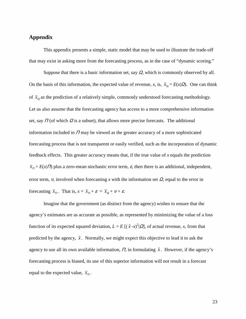
Appendix

This appendix presents a simple, static model that may be used to illustrate the trade-off

that may exist in asking more from the forecasting process, as in the case of “dynamic scoring.”

Suppose that there is a basic information set, say Ω, which is commonly observed by all.

On the basis of this information, the expected value of revenue, x, is, Ωx = E(x|Ω). One can think

of Ωx as the prediction of a relatively simple, commonly understood forecasting methodology.

Let us also assume that the forecasting agency has access to a more comprehensive information

set, say Π (of which Ω is a subset), that allows more precise forecasts. The additional

information included in Π may be viewed as the greater accuracy of a more sophisticated

forecasting process that is not transparent or easily verified, such as the incorporation of dynamic

feedback effects. This greater accuracy means that, if the true value of x equals the prediction

Πx = E(x|Π) plus a zero-mean stochastic error term, ε, then there is an additional, independent,

error term, ν, involved when forecasting x with the information set Ω, equal to the error in

forecasting Πx . That is, x = Πx + ε = Ωx + ν + ε.

Imagine that the government (as distinct from the agency) wishes to ensure that the

agency’s estimates are as accurate as possible, as represented by minimizing the value of a loss

function of its expected squared deviation, L = E [( x -x)2|Ω], of actual revenue, x, from that

predicted by the agency, x . Normally, we might expect this objective to lead it to ask the

agency to use all its own available information, Π, in formulating x . However, if the agency’s

forecasting process is biased, its use of this superior information will not result in a forecast

equal to the expected value, Πx .

24

To make this point concrete, suppose that the agency desires to minimize its own loss

function, Λ = E [γ( x - x - θ)2|Π], where θ represents the bias in its forecasting process. This

would lead to a forecast of Πx +θ. If θ were observable, the bias would present no problem for

the government, which could then make the appropriate adjustment to the agency’s biased

forecast to recover Πx . But, as it may be difficult to know what the inherent forecasting bias is,

it makes sense to treat θ as a random variable from the government’s viewpoint. For simplicity,

we also let the mean of θ equal 0, for, as just shown, the deterministic part of θ is unimportant.

The government faces a difficult choice in deciding whether to let the agency use its

“superior” forecasting process, for this will then also open the door to the inclusion of bias. To

see how different factors affect this trade-off, suppose that the government may influence the

extent to which the agency bases its forecast on Ω, rather than Π, by imposing a penalty on the

agency, P = β( x - Ωx )2, determined by the deviation of the agency’s forecast from that based on

common information. Setting β = 0 will lead the agency to use Π to minimize its own loss

function, Λ, while setting β = ∞ will cause the agency simply to report the common forecast, Ωx .

More generally, its choice of x to minimize the sum of its own loss function and the additional

penalty, Λ+P, will be the weighted average, β’ Ωx +(1-β’ )( Πx +θ), where β’=β/(β+γ) ranges from

0 to 1 as β ranges from 0 to ∞. It is straightforward to show that the value of the relative

penaltyβ’ that minimizes the government’s expected loss function, L, is V(θ)/[V(θ)+V(ν)], the

ratio of the variance of θ to the sum of this variance and the variance of ν.

Thus, the agency should be encouraged to use its superior information, the greater this

informational advantage is (i.e., the larger V(ν) is), and the less unpredictable the influence of

bias on its unobservable forecasting process (i.e., the smaller V(θ) is).

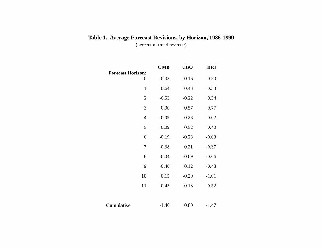
Table 1. Average Forecast Revisions, by Horizon, 1986-1999(percent of trend revenue)

OMB CBO DRIForecast Horizon:

0 -0.03 -0.16 0.50

1 0.64 0.43 0.38

2 -0.53 -0.22 0.34

3 0.00 0.57 0.77

4 -0.09 -0.28 0.02

5 -0.09 0.52 -0.40

6 -0.19 -0.23 -0.03

7 -0.38 0.21 -0.37

8 -0.04 -0.09 -0.66

9 -0.40 0.12 -0.48

10 0.15 -0.20 -1.01

11 -0.45 0.13 -0.52

Cumulative -1.40 0.80 -1.47

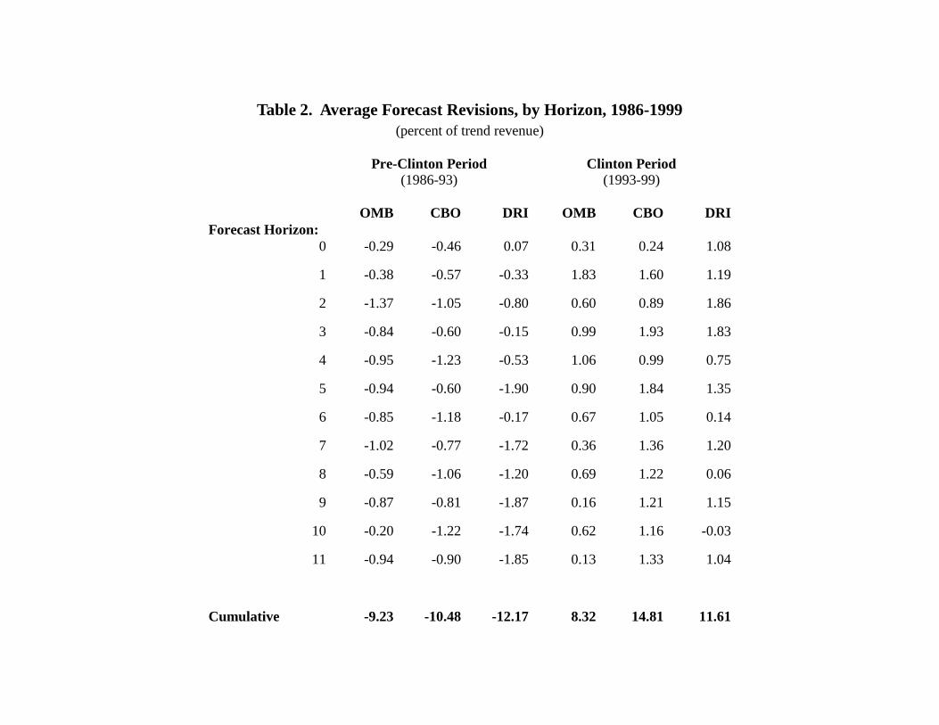
Table 2. Average Forecast Revisions, by Horizon, 1986-1999(percent of trend revenue)

Pre-Clinton Period(1986-93)

Clinton Period(1993-99)

OMB CBO DRI OMB CBO DRIForecast Horizon:

0 -0.29 -0.46 0.07 0.31 0.24 1.08

1 -0.38 -0.57 -0.33 1.83 1.60 1.19

2 -1.37 -1.05 -0.80 0.60 0.89 1.86

3 -0.84 -0.60 -0.15 0.99 1.93 1.83

4 -0.95 -1.23 -0.53 1.06 0.99 0.75

5 -0.94 -0.60 -1.90 0.90 1.84 1.35

6 -0.85 -1.18 -0.17 0.67 1.05 0.14

7 -1.02 -0.77 -1.72 0.36 1.36 1.20

8 -0.59 -1.06 -1.20 0.69 1.22 0.06

9 -0.87 -0.81 -1.87 0.16 1.21 1.15

10 -0.20 -1.22 -1.74 0.62 1.16 -0.03

11 -0.94 -0.90 -1.85 0.13 1.33 1.04

Cumulative -9.23 -10.48 -12.17 8.32 14.81 11.61

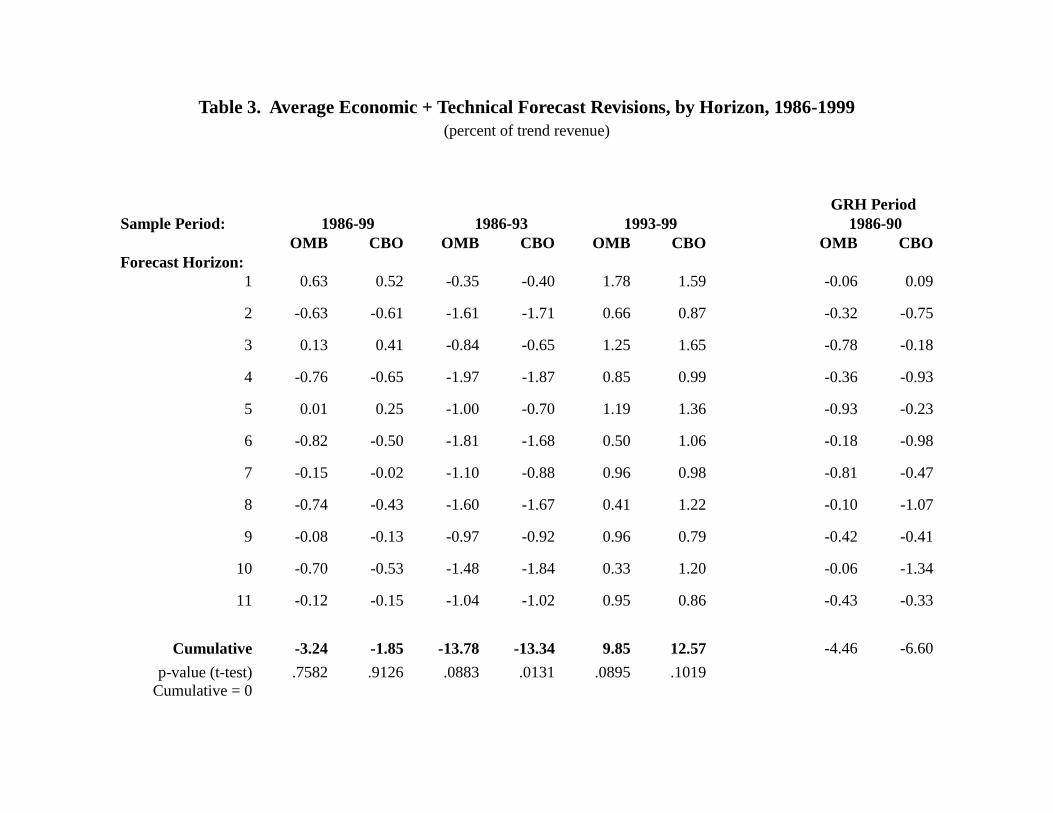
Table 3. Average Economic + Technical Forecast Revisions, by Horizon, 1986-1999(percent of trend revenue)

GRH PeriodSample Period: 1986-99 1986-93 1993-99 1986-90

OMB CBO OMB CBO OMB CBO OMB CBOForecast Horizon:

1 0.63 0.52 -0.35 -0.40 1.78 1.59 -0.06 0.09

2 -0.63 -0.61 -1.61 -1.71 0.66 0.87 -0.32 -0.75

3 0.13 0.41 -0.84 -0.65 1.25 1.65 -0.78 -0.18

4 -0.76 -0.65 -1.97 -1.87 0.85 0.99 -0.36 -0.93

5 0.01 0.25 -1.00 -0.70 1.19 1.36 -0.93 -0.23

6 -0.82 -0.50 -1.81 -1.68 0.50 1.06 -0.18 -0.98

7 -0.15 -0.02 -1.10 -0.88 0.96 0.98 -0.81 -0.47

8 -0.74 -0.43 -1.60 -1.67 0.41 1.22 -0.10 -1.07

9 -0.08 -0.13 -0.97 -0.92 0.96 0.79 -0.42 -0.41

10 -0.70 -0.53 -1.48 -1.84 0.33 1.20 -0.06 -1.34

11 -0.12 -0.15 -1.04 -1.02 0.95 0.86 -0.43 -0.33

Cumulative -3.24 -1.85 -13.78 -13.34 9.85 12.57 -4.46 -6.60

p-value (t-test)Cumulative = 0

.7582 .9126 .0883 .0131 .0895 .1019

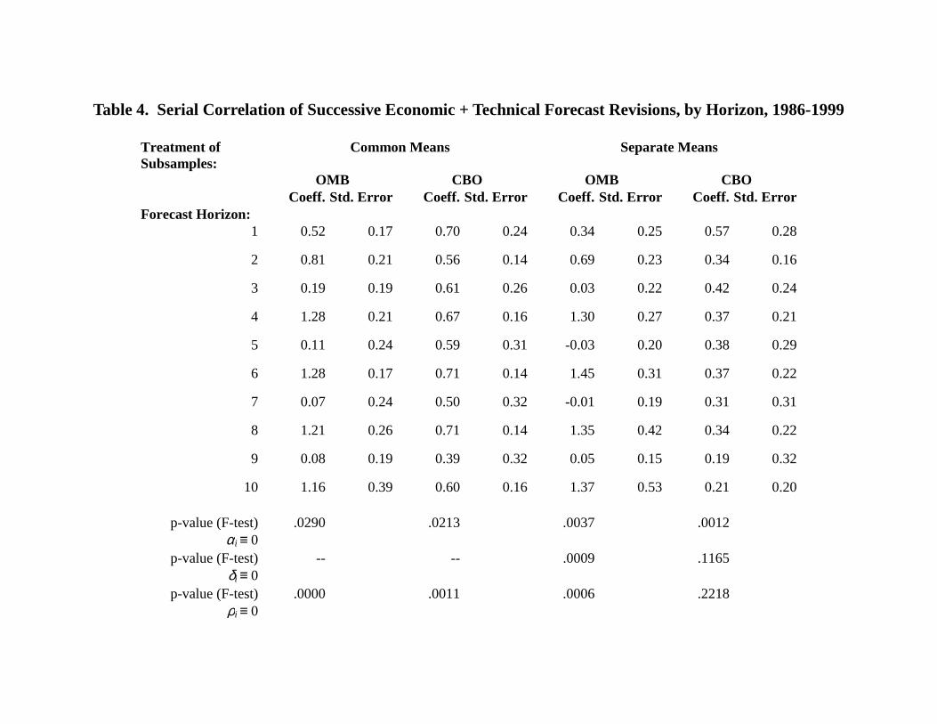
Table 4. Serial Correlation of Successive Economic + Technical Forecast Revisions, by Horizon, 1986-1999

Treatment ofSubsamples:

Common Means Separate Means

OMB CBO OMB CBOCoeff. Std. Error Coeff. Std. Error Coeff. Std. Error Coeff. Std. Error

Forecast Horizon:1 0.52 0.17 0.70 0.24 0.34 0.25 0.57 0.28

2 0.81 0.21 0.56 0.14 0.69 0.23 0.34 0.16

3 0.19 0.19 0.61 0.26 0.03 0.22 0.42 0.24

4 1.28 0.21 0.67 0.16 1.30 0.27 0.37 0.21

5 0.11 0.24 0.59 0.31 -0.03 0.20 0.38 0.29

6 1.28 0.17 0.71 0.14 1.45 0.31 0.37 0.22

7 0.07 0.24 0.50 0.32 -0.01 0.19 0.31 0.31

8 1.21 0.26 0.71 0.14 1.35 0.42 0.34 0.22

9 0.08 0.19 0.39 0.32 0.05 0.15 0.19 0.32

10 1.16 0.39 0.60 0.16 1.37 0.53 0.21 0.20

p-value (F-test)αi ≡ 0

.0290 .0213 .0037 .0012

p-value (F-test)δi ≡ 0

-- -- .0009 .1165

p-value (F-test)ρi ≡ 0

.0000 .0011 .0006 .2218

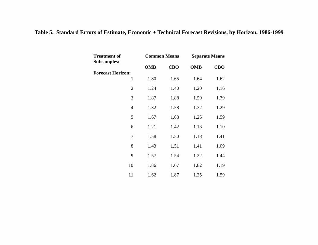
Table 5. Standard Errors of Estimate, Economic + Technical Forecast Revisions, by Horizon, 1986-1999

Treatment ofSubsamples:

Common Means Separate Means

OMB CBO OMB CBOForecast Horizon:

1 1.80 1.65 1.64 1.62

2 1.24 1.40 1.20 1.16

3 1.87 1.88 1.59 1.79

4 1.32 1.58 1.32 1.29

5 1.67 1.68 1.25 1.59

6 1.21 1.42 1.18 1.10

7 1.58 1.50 1.18 1.41

8 1.43 1.51 1.41 1.09

9 1.57 1.54 1.22 1.44

10 1.86 1.67 1.82 1.19

11 1.62 1.87 1.25 1.59

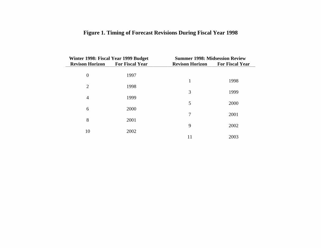
Figure 1. Timing of Forecast Revisions During Fiscal Year 1998

Winter 1998: Fiscal Year 1999 Budget Summer 1998: Midsession ReviewRevison Horizon For Fiscal Year Revison Horizon For Fiscal Year

0 19971 1998

2 19983 1999

4 19995 2000

6 20007 2001

8 20019 2002

10 200211 2003