on the forecasting of the challenging world future scenarios

Technological Forecasting & Social Change 78 (2011) 1445–1470

Contents lists available at ScienceDirect

Technological Forecasting & Social Change

On the forecasting of the challenging world future scenarios

Luiz C.M. Miranda a,⁎, C.A.S. Lima b

a Instituto Nacional de Pesquisas Espaciais, São José dos Campos, SP, Brazilb Universidade Estadual de Campinas, Campinas, SP, Brazil

a r t i c l e i n f o

⁎ Corresponding author at: Rua Serimbura 60 403-AE-mail address: [email protected] (L.C.M. Mira

0040-1625/$ – see front matter © 2011 Elsevier Inc.doi:10.1016/j.techfore.2011.04.001

a b s t r a c t

Article history:Received 29 October 2010Received in revised form 30 March 2011Accepted 5 April 2011Available online 7 May 2011

Logistic and power law methodologies for both retrospective and prospective analyses ofextended time series describing evolutionary growth processes, in environments with finiteresources, are confronted. While power laws may eventually apply only to the early stages ofsaid growth process, the Allee logistic model seems applicable over the entire span of a longrange process. On applying the Allee logistic model to both the world population and the worldgross domestic product time series, from 1 to 2008 AD, a projection was obtained that along thenext few decades the world should experience a new economic boom phase with the worldGDP peaking around the year 2020 and proceeding from then on towards a saturation value ofabout 142 trillion international dollars, while the world population should reach 8.9 billionpeople by 2050. These results were then used to forecast the behavior of the supply andconsumption of energy and food, two of the main commodities that drive the world system.Our findings suggest that unless the currently prevailing focus on economic growth is changedinto that of sustainable prosperity, human society may run into a period of serious economicaland social struggles with unpredictable political consequences.

© 2011 Elsevier Inc. All rights reserved.

Keywords:Evolutionary growth processesLogistic model forecastingAllee modified logistic modelWorld population forecastingWorld GDP evolutionFood supply evolutionPrimary energy forecasting

1. Introduction

One of the main concerns mankind faces today regards the sustainability of life in our planet as a result of an unprecedentedfast growth that the relevant socioeconomic indicators have been signaling since the beginning of the last century. This has posed amulti-faceted question encompassing practically all dimensions of human activity, which has no simple answer. The growinginterest on this subject dates back to the post World War II period. In the aftermath of this worldwide conflict, the strategicintelligence doctrine became a central aspect of the foreign policy of leading nations, especially along the Cold War period. In TheYear 2000, a book published in 1967, Kahn andWiener [1] account for that in detail. With some success in a few cases, they presentfuturistic projections on a wide range of themes including world demography and economy, science and technology, food supply,and social changes among others. Some of the earlier literature on the subject is also reviewed in this work.

In parallel, and independently, by the late 1960's and the beginning of the 70's a new and broader theoretical framework forsocial analysis, the world system theory, was proposed by Wallerstein [2], Modelski [3] and Frank [4], among other renownedresearchers. Further references and a more recent account of the world system can be found in Modelski and Denemark [5]. Theworld system theory besides providing a new framework for interpreting the evolution of human society, offered also a newmeans of forecasting the challenging global issues that one currently faces.

From a holistic perspective the evolution of human society results from the mutually interfering combination of the differentevolutionary paths followed by each of its various dynamic components (politics, finances, trade, science, technology, industrial

, 12243-360, S. J. Campos, S. Paulo, Brazil. Tel.: +55 12 33222333.nda).

All rights reserved.

http://dx.doi.org/10.1016/j.techfore.2011.04.001

mailto:[email protected]

http://dx.doi.org/10.1016/j.techfore.2011.04.001

http://www.sciencedirect.com/science/journal/00401625

1446 L.C.M. Miranda, C.A.S. Lima / Technological Forecasting & Social Change 78 (2011) 1445–1470

innovation, and so on) acting synergistically to build and shape it up. Given this multi-variable complexity of the world evolution,it is inevitable that one narrows this spectrum of variables when forecasting future world scenarios, by making appropriatechoices. For the problem of the sustainability of life in our planet, focused in this work, theworld population unquestionably comesin as themost important variable. After all, it constitutes themain actor in such a process. In fact, the abilities to understand Nature(science), partially dominate it (technology) and transmitting and improving the acquired knowledge in a continuous feedbackprocess is certainly the most important characteristics that made our species a singular one among all others in the planet. Nomatter which dimension one chooses to check the evolution of mankind, whether economical, social or political, the main driverfor it lies invariably on the existing knowledge content.

Second to the population, the world gross domestic product (GDP) as a measure of the human activity output is certainlyanother important variable to be considered in this context. Going a step further in this hierarchy, we should next consider theevolutionary paths of some basic commodities (such as energy, water, transportation, and food supply) that backed up theachievement of this output. In fact, forecasting what will be the pressures upon them in the future will be highly instrumental fortechnology intelligence and planning aiming at sustaining our society in the future. Last but not least, and perhaps the mostchallenging variable, regards the political demands. The evolution of these variables will most certainly call upon new worldpolicies, so that workable solutions can be construed from the envisaged forecasted trends. Inevitably, should preserving ourspecies be the ultimate goal, some new compromised policies and economic ordering will have to be agreed upon.

The ongoing discussions on the development of the world economy vis a vis the finite resources of our planet in severalinternational forums are already producing some alternatives which sooner or later ought to be more closely evaluated. Theprevailing economic policies are geared, above all, to economic growth. Two objectives other than growth, namely, sustainabilityand wellbeing, havemoved up into both the political and the policy-making international agenda in recent years, thus challengingthe overriding priority traditionally given to economic growth. The concept of prosperity without growth, detailed in the recentbook by Jackson [6], is certainly applicable to some of the more advanced nations, e.g., the Scandinavian countries. In contrast, indeveloping countries economic growth is still badly needed. Yet, this does not necessarily mean that these countries should seekeconomic growth at any price. Economic growth policies there could, alternatively, be geared through implementing developmentprojects that minimize negative economic externalities. Further discussion and references on economic externalities and growthcan be found, for instance, in Ref. [7].

To strengthen the arguments regarding the probably unsustainable pace at which the world economy has been currentlygrowing we present in Table 1 the values of the world GDP and world population in some selected years from 1 to 2008 AD. Thedata listed in Table 1 were taken from Maddison's [8] historical statistics for the world economy.

The figures in Table 1 clearly show the jump in the rate at which human society has been growing since the 19th century. Thisvertiginous growth is intimately linked to the advancement of knowledge that took place in the Modern Era, as has been recentlypointed out by Miranda and Lima [9]. Using two time series spanning the last five centuries (1500 to 1999), consisting of 1499 and401 entries for themost impacting scientific discoveries and technological inventions, respectively, these authors have shown thatworld GDP is exponentially correlated with both the scientific discoveries and the technological inventions. In Fig. 1 wereproduced their plot of the evolution of the world GDP as a function of the cumulative number of scientific discoveries (curve a)and the cumulative number technological inventions (curve b).

This figure shows that, except for three decades around World War I, the Great Depression and World War II, in which theworld GDP underwent a well known stagnation, the logarithm of the GDP displays a linear correlation with the accumulatednumber of both scientific and technological most impacting events. We should remark here that the vast majority of theselected entries for the scientific discoveries and technological inventions, covering the last five centuries, ended up beingrelated to events that took place within the group of countries comprisingWestern Europe, USA, Canada and Japan. Accordingly,for the purposes of the correlations shown, the GDP considered in the plots depicted in Fig. 1 is the compound GDP for thatgroup of countries.

Formore than 40 years the time evolution of several socioeconomic indicators has been intensively investigated by a number ofresearchers [9–15,23,24,27] using mostly the logistic approach to modeling their growth processes. More recently and probablymotivated by the politically and economically disturbing period that characterized the last 10 years or so, there has been arenewed interest in the forecasting of world economy. Logistic modeling [16,17], models based upon power laws [18,19], and thedynamic models of Kremer [20] and Korotayev et al. [21] have also been applied to accomplishing such endeavor. Furtherreferences on the subject can be found in Ref. [22].

Table 1World GDP and population at selected years during Christian era. For each variable we list both its actual value as well as its ratio with respect to the previous date.

Date(Calendar year)

Population(in billion inhabitants)

GDP(in trillion 1990 International Gery–Khamis dollars)

Value Ratio Value Ratio

1 0.226 0.1051500 0.438 1.9 0.248 2.41820 1,042 2.4 0.694 2.81900 1.563 1.5 1.972 2.82000 6.077 3.9 36.688 18.6

Fig. 1. Log-linear plot of the GDP vs. the cumulative number of events: curve (a) refers to the most impacting scientific discoveries and curve (b) to the mostimpacting technological inventions.

1447L.C.M. Miranda, C.A.S. Lima / Technological Forecasting & Social Change 78 (2011) 1445–1470

In this paper we apply our recently proposed methodology for the logistic analysis of evolutionary growth processes [23,24] tothe forecasting of global economy trends and compare the results obtainedwith some of those in the above cited works. The paperis organized as follows. In the next section we briefly review themain aspects of both the logistic and power lawmodeling in orderto set the stage for comparative analysis of the results. The following two sections are dedicated to the presentation of the resultsfor world population and GDP, respectively. A comparative analysis and a discussion on the implications of these results on thefuture supply of some basic commodities then follow. Overall, the underlying focus is that of discussing, both retrospectively andprospectively, the quest for a sustainable economic growth to preserve the ecological balance in the planet.

2. Logistic and power laws models

In quite general terms, the time evolution of a growth process characterized by a variable N is governed by a rate equation ofthe type,

dNdt

= N⋅F Nð Þ; ð1Þ

F(N) describes the net percent, or per capita, growth rate that regulates the process. Depending on the nature of the
whereself-regulation, F(N) may assume different functional forms depending on the nature of the self-regulating mechanismsinvolved.
For systems having a finite carrying capacity K, determined by the existence of finite resources, the self-regulation for a growthprocess should satisfy two conditions, namely, (i) — be positive for 0bNbK, and (ii) — be such that

dFdN

≤0

values of time. In contrast, in the case of unlimited, or uncontrolled, growth processes, dF/dNN0 indicating the presence of a
for allcatastrophic process.
For the Verhulst logistic equation F(N) consists of a compensatory term of the type,

F Nð Þ = r⋅ 1−NK

� �; ð2Þ

r denotes the growth parameter. Eq. (2) simply expresses the assumption that competition for fixed resources will always
whereincrease as the number of competitors increases. Substituting Eq. (2) into Eq. (1) the resulting rate equation for N consists of asynchronous replication term proportional to N and a compensatory growth inhibition term proportional to N 2, whose solution isthe well-known logistic function which can be written as
N tð Þ = Ker t−tcð Þ

1 + e r t−tcð Þ : ð3Þ

In Eq. (3) tc denotes the inflection point of the logistic function excursion at which it reaches half the value of K.


In the case of uncontrolled growth process the most common functional form for F(N) is that of a power law, namely,

Fig. 2. Dcurves

F Nð Þ = 1γ⋅Nα

; ð4Þ

ich α denotes the exponent governing the growth process and γ−1 is a growth rate parameter. We note that for α=0 the
in whpower law growth process reduces to the well-known Malthusian law. Examples of uncontrolled growth are common amongcertain biological species populations due to the absence there of a technology intelligence (viewed as the capacity to at leastpartially dominate Nature). Probably the best known example of that is the phytoplankton population explosion, the so-calledalgae blooms, occurring in coastal waters.
Integrating Eq. (4) from an initial time ti at which N=Ni to a time t one gets the following hyperbolic law for the time evolutionof N:

N tð Þ = αγð Þ1=αt0−tð Þ 1 =α

; ð5Þ

the critical time to is defined as t0= ti+(α γ Niα)−1. It represents the time at which the power law growth process diverges
where
to infinity.The Verhulst logistic model as presented in the foregoing assumes a synchronous replication at all stages of the growth process.

This is a weak point in this model when describing certain processes, as noted by Allee [25] some 80 years ago, in regards to thedynamics of biological populations. In his investigations on the animal reproduction, Allee observed that, for some organisms,finding a suitable mate may pose some difficulties at low population stages. A more realistic description of replication, in this case,would then be to assume that the population growth scales as N 2 rather than linearly. This is in essence what became known asthe Allee effect. In the context of biological population dynamics, it consists in introducing a component of reproductive fitness (orfertility) represented by an increasing function of N. A simple example for this fitness component formulation is that proposed byFowler and Ruxton [26] which consisted in writing it as a bounded exponential function of the type 1−exp (−N/Nc), whereNc is apositive constant associated with the low population reproductive threshold.

In a previous paper [24] we have discussed the introduction of the Allee effect into the logistic model and applied it to the caseof the human population evolution. That was done by writing the modified logistic equation as

dNdt

= rNϕ Nð Þ 1−NK

� �; ð6Þ

the function ϕ(N) represents the Allee fitness component. The only requirement that this function should satisfy is that it
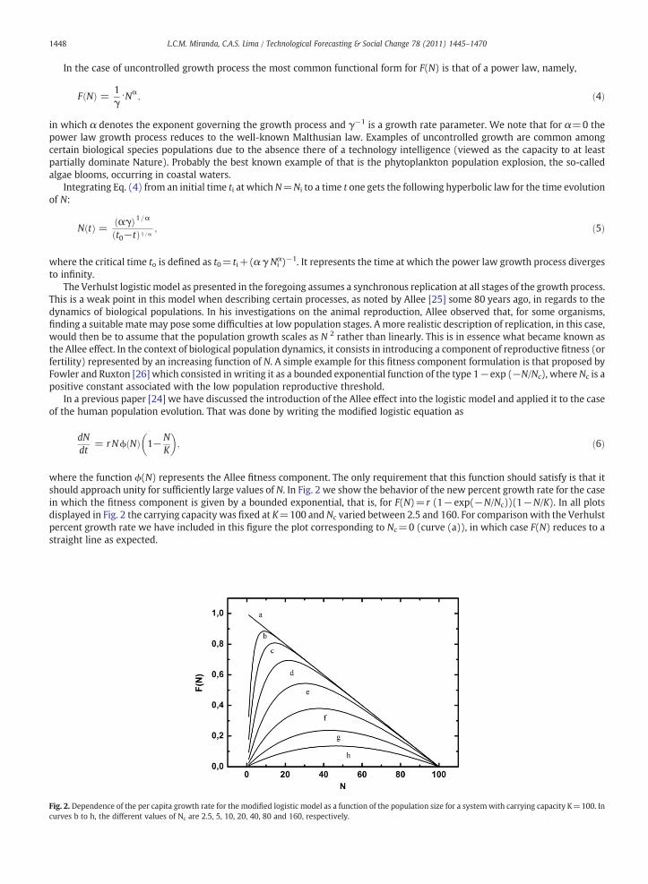
whereshould approach unity for sufficiently large values of N. In Fig. 2 we show the behavior of the new percent growth rate for the casein which the fitness component is given by a bounded exponential, that is, for F(N)=r (1−exp(−N/Nc))(1−N/K). In all plotsdisplayed in Fig. 2 the carrying capacity was fixed at K=100 and Nc varied between 2.5 and 160. For comparison with the Verhulstpercent growth rate we have included in this figure the plot corresponding to Nc=0 (curve (a)), in which case F(N) reduces to astraight line as expected.
ependence of the per capita growth rate for the modified logistic model as a function of the population size for a system with carrying capacity K=100. Inb to h, the different values of Nc are 2.5, 5, 10, 20, 40, 80 and 160, respectively.

image of Fig.�2


The curves in Fig. 2 clearly exhibit the shape of a distorted peak, such that as N approaches the carrying capacity they tendtowards a compensatory behavior following a straight line with negative slope. At low values of N, in contrast, they behave as ifthey were in a purely replication regime, increasing as N increases.

Even though the modification of the logistic equation discussed in Ref. [24] was carried out in the context of populationdynamics, it is equally applicable to the analysis of the time evolution of other socioeconomic indicators. For instance, in Ref. [27]we have applied the Allee modified logistic methodology, outlined above, to the analysis of quite a distinct indicator, namely, theannual evolution of cars fleets.

3. World population

Let us consider the applications of power law and logistic models to the analysis of the human population evolution. We beginwith the power law modeling, by referring to the paper by Johansen and Sornette [19] in which the accelerating growth of theworld population, GDP and of some financial indicators are discussed. Their main conclusion, which has been replicated in a recentpaper by Devezas [17], is that the human population and its economic output (represented by the world GDP) are growingaccording to what they call a super-Malthusian mode. In both works, the accelerating growth rates are shown compatible with aspontaneous singularity which they forecast should take place at the same critical year, namely, 2052±10, signaling to theoccurrence of an abrupt transition to a new regime. We recall that, within the same context, some 50 years ago, von Foerster et al.[28], assuming a power law of the type given in Eq. (5) with exponent α set to unity, predicted an economic doomsday to occur atNovember 13th, 2006.

To make the forthcoming remarks self-contained, let us recall Johansen and Sornette formulation, repeated in Section 11 ofDevezas' work [17], following an ansatz previously proposed by Cohen (see Ref. 1 in Ref. [19]), summarizing it as follows: startingwith a logistic equation written as

Fig. 3.Win Ref. [

dNdt

= rN tð Þ K−N tð Þ½ � ð7Þ

thors in Refs. [17] and [19] argue that if KNN(t), then N(t) explodes to infinity, after a finite time, creating a singularity. They
the auproceed arguing that in this case the term— N(t) in the square bracket can be dropped out, and by assuming for K a simple power-law dependence in N, i.e., K∝N α, the logistic equation reduces to
dNdt

= r N tð Þ½ �1 + α: ð8Þ

The solution to this type of equation has been analyzed in the previous section and is given by the expression in Eq. (5) if wejust replace there γ=r−1. As shown there, the generic consequence for a power law governing the growth rate is the appearanceof a singularity at a critical time t0. In Ref. [19] this time is estimated to be 2052±10 for both the world population and GDP. Incontrast, in Ref [17] the value found for the GDP critical time is about the year 2100.

Now, let us take a closer look in the arguments used in those papers leading to the above power law behavior. We start bymaking three important remarks. Firstly, from a purely mathematical point of view, no matter the size of K, Eq. (7) says that the

orld population per capita growth rate evolution from 1 to 2008 AD. Curve (a) corresponds to the percent growth rate calculated using the result obtained19] for N(t), whereas curve (b) represents the result obtained from the data fitting to the Allee modified logistic model.

image of Fig.�3

Table 2Values of the estimated parameters of a single logistic function fitting to the two world population data sets used in this work, using two distinct software, asdetailed in the text.

Origin 8.0

Maddison data US Census Bureau data

Value Error Value Error Value Error Value Error

A0 1.248 0.045 0 – 1.310 0.477 0 –

K 7.952 0.144 12.282 0.282 7.691 0.145 12.023 0.287tc 1989.467 0.411 2000.811 1.686 1988.443 0.401 1999.161 1.748τ 23.902 0.428 36.877 0.439 23.185 0.444 36.495 –

Δt 105.036 162.054 101.885 160.375R2 0.9999 0.9999 0.9999 0.9996RSSQ 0.0061 0.0341 0.0076 0.0408

Loglet 2

Value Error Value Error

A0 0 – 0 –

K 12.292 0.277 12.032 0.236tc 2000.873 1.333 1999.218 1.417τ 36.897 – 36.513 –

Δt 162.141 160.456RSSQ 0.0341 0.0408

Fig. 4. Single logistic function modeling of the world population time evolution. The solid line in the plot represents the data fitting for the period from 1950 to2008, leaving A0 as an adjustable parameter, as well as its extrapolation towards both the past (1850) and the future (2100). The dashed line, on the contrarycorresponds to an equivalent fit and extrapolation but with the offset parameter A0 set both fixed and equal zero.


populationwill always reach this value at sufficiently large times. This is evident in the plot of the percent growth rate as a functionof N, as shown for instance in Fig. 2. The singularity of the logistic equation is by no means related to K, but rather to size of thegrowth parameter r. This is best seen whenworking with the logistic equation in discrete time, which is a classical model examplein chaos theory. For continuous time, Eq. (7) is singular only for r→∞, in which case it reduces to the well known Heaviside stepfunction. In this limiting situation the logistic equation exhibits a finite discontinuity at the inflection point.

Secondly, the argument used by these authors to neglect N(t) as compared to K in the bracket in Eq. (7) is only valid in theinitial stages of the growth process. As discussed in Section 2 in connection to the Allee effect, this corresponds to the reproductive,or depensation, regime of the growth process. Consequently, using this approximation and extrapolating the results so obtained toinfer the population behavior far from the early stages may produce misleading conclusions.

Thirdly, if one assumes the world population growth to be described by Eq. (8), its percent growth rate will always be amonotonically growing function ofN, a behavior that is not compatible with the existingworld population data. Towit, we show inFig. 3 the percent growth rate of Maddison world population data as a function of its population from 1 to 2008 AD. Curve (a) inFig. 3 corresponds to the percent growth rate calculated using the result obtained in Ref. [19] for N(t), namely,

N tð Þ = 16242056−tð Þ1:4 : ð9Þ

,

image of Fig.�4


Curve (b), on the other hand, represents the result we have obtained from the data fitting to our Allee modified logistic growthrate function as discussed in Ref. [24], which we refer to for details on the calculations. This allowed us to forecast a worldpopulation carrying capacity of 11.4 billion inhabitants, with an inflection point at 1987.5. By the year 2050 the estimated worldpopulation reported in Ref. [24] was of 8.9 billion people, in good agreement with the prediction of 9.1 billion people reported bythe UN 2008 Population Prospect Revision [29] for that year. Nevertheless, the point to be emphasized here, and clearly evident inFig. 3, is that the power law model may eventually prove to be a suitable model only under the conditions of low populationregime. At high populations it diverges and fails to reproduce the existing data trend.

As to the use of the standard Verhulst logistic modeling for forecasting the world population, Boretos [16] has recently reportedthe results of his calculations using the US Census Bureau population data set [29] spanning from 1950 until 2005. The calculationswere carried out using a single logistic function with an added, fixed, off set. His results indicate a world population carryingcapacity of 8.99 billion people with an inflection point at the year 1995, and a characteristic process duration time, Δt, (the lapsefor N to grow from 10% to 90% the carrying capacity) equal to 117.5 years. Similar calculations were later reported by Devezas [17]using, however, the more recent US Census Bureau data set spanning from 1950 to 2009. Even though this paper neither informson important details about the performed calculations nor reports the corresponding numerical results, we gather from the textthat the author arrives at a carrying capacity of about 12 billion people with characteristic duration time of the order of 160 yearsand an inflection point lying between 2000 and 2001.

For comparisons sake, we then decided to carry on also an equivalent single logistic modeling of the world population usingboth of the available time series, namely, Maddison's and the US Census Bureau data sets. The data fitting was carried out usingtwo distinct software, namely, the Origin 8.0® from OriginLab Corporation and the Loglet Lab 2 [30]. The model function was thatgiven by Eq. (3) to which we added a fourth off set adjustable parameter, A0. In Table 2 we summarize the results from the datafitting procedures for the two data sets using both software.

An overall aspect that emerges from both Table 2 and Fig. 4 is that the results of the data fitting procedures for both data setsare practically the same. The major difference between the two reported fits occurs when the offset parameter A0 is both fixedand set equal to zero or is left as a free adjustable parameter. When letting the offset as an adjustable parameter the finalcarrying capacity is given by the sum A0+K. For this case our calculations, as summarized in Table 2, point to a final carryingcapacity of about 9.2 billion people, for Maddison's data base and of about 9 billion people for the case of the US Census Bureaudata base.

To check for possible longer range series differences between the two fitting procedures, we have plotted in Fig. 4 the results ofthe data fitting of Maddison's world population data using the Origin 8.0 software. For comparison, we have included in this plot allof Maddison's data points from 1820 onwards. Fig. 4, as well as the results summarized in Table 2, clearly demonstrates that thebest procedure when fitting to a truncated database (in this case, the world population from 1950 to 2008) is to allow for anadjustable offset parameter in addition to the usual adjustment of the three-parameter logistic function, avoiding, accordingly,undesirable over-estimated values for the logistic parameters.

Notice that the solid line in Fig. 4, corresponding to the single logistic data fitting of Maddison's population database from 1950to 2008, with an adjustable offset parameter exhibits an inflection at 1989.5. This is quite consistent with the result obtained fromthe percent growth rate data fitting to an Allee effect modified logistic growth model function in the range from 1 to 2008 AD,where an inflection at 1987.5 was obtained, as discussed earlier in this section. However, in regards to the predicted value for theworld population carrying capacity of about 9.2 billion people, this figure lies well below the 11.4 billion people value forecastedby the other modeling procedure. This discrepancy seems to be associated with the limited time range considered in the singlelogistic modeling (1950–2008) shown in Fig. 4, as compared to the (1 to 2008) time scale used in the Allee effect modified logisticgrowth model.

Fig. 5. Correlation plot of the world GDP and population corresponding to the entire period of time of Maddison database, namely, from 1 to 2008 AD. The solid linecorresponds to thedatafitting to a two-logistic growthmodel. The inset includes the extrapolationof thedatafittedmodel function towards larger (future) population sizes.

image of Fig.�5

Table 3Values of the characteristic parameters obtained from the two-logistic data fitting to the world GDP in trillion 1990 International Geary–Khamis dollars.

Parameters Phase 1 Phase 2

Ai 26.608 115.942Nci 3.682 7.508δi 0.826 0.644RSSQ (residual sum of squares) 4.621R2 0.9996

Fig. 6. World GDP time evolution as obtained from the substitution into Eq. (10) of our previously reported Allee logistic model solution for the world populationtime evolution [24]. The values of the parameters appearing in Eq. (10) are those listed in Table 3.


4. World GDP

In the last 40 years or so, evidences have been reported [10–15] supporting the argument that the carrying capacity ofsocioeconomic and human performance indicators are frequently determined by the status of the scientific and technologicalknowledge attained at the considered period by the corresponding social group. As knowledge advances, new processes andproducts are introduced changing the dynamics of society as a whole thus promoting it into a new stage of development.Accordingly, it seems natural to expect that such evolutionary path should encompass a sequence of learning curves reflecting theinterplay among the several social, economical, technological and political components that gear the human society evolution.Consequently, the analysis of a long range time series of a given socioeconomic indicator usually calls for a multi-logisticdescription. The analysis of the world GDP presented in this section is no exception to this point.

Since human population is the main driver of the important transformations that have been taking place in our planet along itshistory, we begin our analysis by considering more closely the relationship between the evolution of world's GDP and population.The GDP and world population data used in our analysis was taken from Maddison [8] historical statistics of the world economy,and their correlation was modeled by writing it as

G = ∑i=1

Aie N−Ncið Þ=δi

1 + e N−Ncið Þ= δi : ð10Þ

In Eq. (10), G denotes the world GDP, Ai denotes the excursion towards saturation during the i-th logistic growth sequence, Nci

is the population where the inflection point occurs in sequence i with a growth rate parameter (currency per inhabitant) δi−1. InMaddison data sets, the GDP are expressed in constant 1990 US dollars converted at international Geary–Khamis (G–K)purchasing power parities [8], which, in what follows, we shall occasionally refer to as international dollars.

In Fig. 5 we plot the world GDP and population correlation data corresponding to the entire period of time covered byMaddison database, namely, from 1 to 2008 AD. The solid line corresponds to the data fitting to a multi-logistic function. It wasfound that in this case the best fit occurred for a two-logistic growth model, whose values of the fitting parameters are listed inTable 3. In the inset, we replot the GDP correlation but now extending into the future the data fitted model function.

From a broader standpoint, Fig. 5 may be viewed as a representation of the general input–output response function of thehuman society, in which the input is the human population and the output is the overall human product, represented by the worldGDP. It tells us that the human society output is governed by a nonlinear response function whose dynamics is that of a generallogistic equation. It also indicates that the evolution of the world GDP from 1 to 2008 AD is essentially characterized by a broad

image of Fig.�6

Fig. 7. Time evolution since 1955 of the world trade exports value and volume indicating that from 1995 on the world trade exports value has entered a phase oexplosive growth as compared to the exports volume.

Fig. 8. World GDP per capita growth rate evolution from 1 to 2008 AD. The solid black line represents the results from the present GDP time evolution modelingThe gray line corresponds to a coarser analysis of the per capita growth rate assuming that the GDP is described by a single Verhulst logistic function, in which caseit decreases linearly with increasing GDP.


f

phase centered around a population of about 3.68 billion people (occurring at approximately the year 1970), and predicts a secondphase peaking at a population of the order of 7.51 billion people, after which the GDP should approach a saturation value of theorder of 142 trillion international dollars, at a faster rate than that observed in phase 1. Now, if the above input–output modelrepresents an adequate general description of the evolution of the world GDP, then upon substituting into Eq. (10) a modelfunction expressing the time evolution of the world population, wemay be able to the recover the explicit time dependence of theevolution of the GDP that can be compared with the existing data. This procedure provides us a double check on the proposeddescription of the GDP evolution, namely, a check not only on the adequacy of Eq. (10) to model the societal response function butas well as a check on the eventual world population model function we choose to use on this testing. We have carried it out usingas a model function for the world population our previously reported [24] solution to the Allee modified logistic equation,henceforth denoted as ALM solution. The results are shown in Fig. 6.

The very good description of the time evolution of the world GDP shown in Fig. 6 confirms the adequacy of both the input–output modeling of the societal response as well as the Allee-logistic model [24] of the world population time evolution.Furthermore, the results shown in Fig. 6 also show that the second phase of economic growth theworld GDP forecasted by the GDPand world population correlation (cfe. Fig. 5 and Table 3) should go through to a peak by the year 2020, corresponding to apopulation of about 7.51 billion people. It might be remarked that this result is in quite good agreement with a previouslypredicted peak for the 5th K-wave [31], as well as with Modis' [32] previous forecast of a forthcoming economic boom to bepeaking around the mid-2020s, from his analysis of the historical data on energy consumption.

Fig. 6 also forecasts a GDP carrying capacity of about 142 trillion 1990 international dollars, to be reached by the beginning ofthe next century. By 2050 the GDP is forecasted to be of the order of 132 trillion international dollars, roughly 2.6 times its 2008value. Overall, these results seem to indicate an ongoing unprecedented phase of fast and intense economic growth. This phase offast and intense economic growth may sound, in principle, too optimistic. However, it gains further support from the analyses of

.

image of Fig.�7

image of Fig.�8

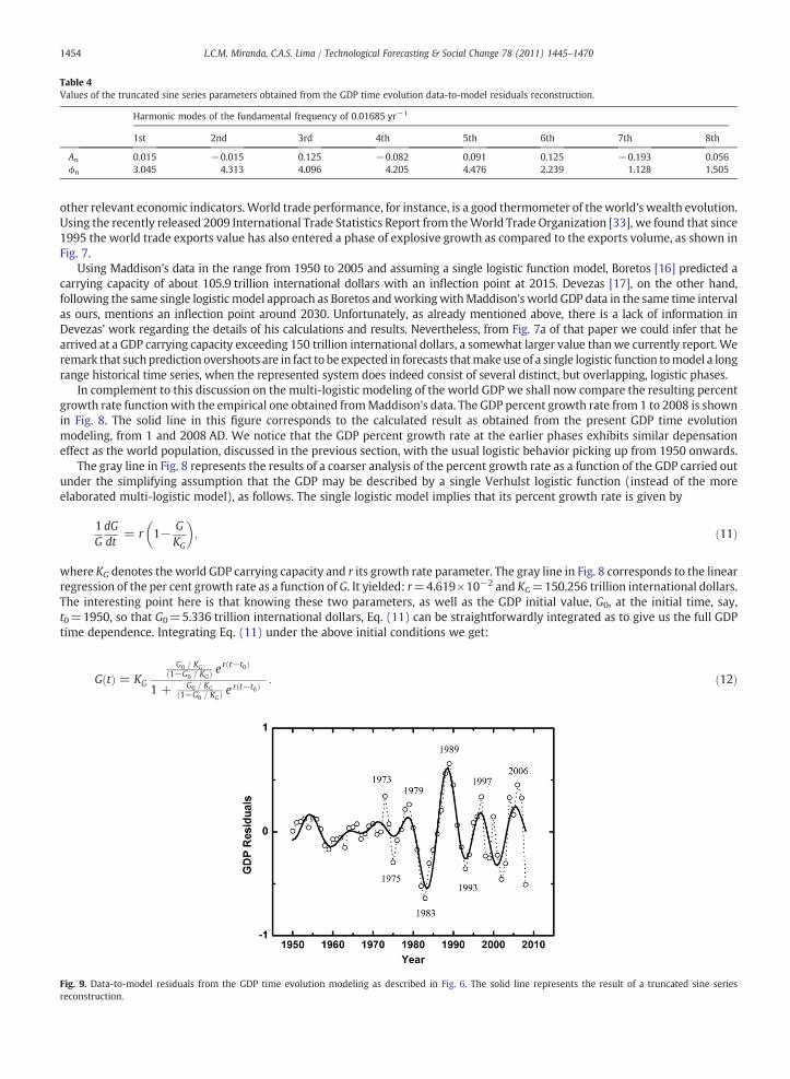
Table 4Values of the truncated sine series parameters obtained from the GDP time evolution data-to-model residuals reconstruction.

Harmonic modes of the fundamental frequency of 0.01685 yr−1

1st 2nd 3rd 4th 5th 6th 7th 8th

An 0.015 −0.015 0.125 −0.082 0.091 0.125 −0.193 0.056ϕn 3.045 4.313 4.096 4.205 4.476 2.239 1.128 1.505


other relevant economic indicators. World trade performance, for instance, is a good thermometer of the world's wealth evolution.Using the recently released 2009 International Trade Statistics Report from theWorld Trade Organization [33], we found that since1995 the world trade exports value has also entered a phase of explosive growth as compared to the exports volume, as shown inFig. 7.

Using Maddison's data in the range from 1950 to 2005 and assuming a single logistic function model, Boretos [16] predicted acarrying capacity of about 105.9 trillion international dollars with an inflection point at 2015. Devezas [17], on the other hand,following the same single logistic model approach as Boretos andworkingwithMaddison's world GDP data in the same time intervalas ours, mentions an inflection point around 2030. Unfortunately, as already mentioned above, there is a lack of information inDevezas' work regarding the details of his calculations and results. Nevertheless, from Fig. 7a of that paper we could infer that hearrived at a GDP carrying capacity exceeding 150 trillion international dollars, a somewhat larger value thanwe currently report. Weremark that suchprediction overshoots are in fact to be expected in forecasts thatmakeuse of a single logistic function tomodel a longrange historical time series, when the represented system does indeed consist of several distinct, but overlapping, logistic phases.

In complement to this discussion on the multi-logistic modeling of the world GDP we shall now compare the resulting percentgrowth rate function with the empirical one obtained fromMaddison's data. The GDP percent growth rate from 1 to 2008 is shownin Fig. 8. The solid line in this figure corresponds to the calculated result as obtained from the present GDP time evolutionmodeling, from 1 and 2008 AD. We notice that the GDP percent growth rate at the earlier phases exhibits similar depensationeffect as the world population, discussed in the previous section, with the usual logistic behavior picking up from 1950 onwards.

The gray line in Fig. 8 represents the results of a coarser analysis of the percent growth rate as a function of the GDP carried outunder the simplifying assumption that the GDP may be described by a single Verhulst logistic function (instead of the moreelaborated multi-logistic model), as follows. The single logistic model implies that its percent growth rate is given by

Fig. 9.reconst

1GdGdt

= r 1− GKG

� �; ð11Þ

KG denotes the world GDP carrying capacity and r its growth rate parameter. The gray line in Fig. 8 corresponds to the linear
whereregression of the per cent growth rate as a function of G. It yielded: r=4.619×10−2 and KG=150.256 trillion international dollars.The interesting point here is that knowing these two parameters, as well as the GDP initial value, G0, at the initial time, say,t0=1950, so that G0=5.336 trillion international dollars, Eq. (11) can be straightforwardly integrated as to give us the full GDPtime dependence. Integrating Eq. (11) under the above initial conditions we get:
G tð Þ = KG

G0 = KG1−G0 = KGð Þ e

r t−t0ð Þ

1 + G0 = KG1−G0 = KGð Þ e

r t−t0ð Þ : ð12Þ

Data-to-model residuals from the GDP time evolution modeling as described in Fig. 6. The solid line represents the result of a truncated sine seriesruction.

image of Fig.�9

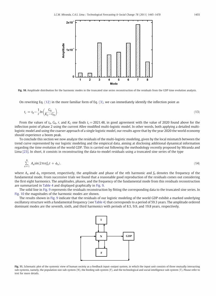
Fig. 10. Amplitude distribution for the harmonic modes in the truncated sine series reconstruction of the residuals from the GDP time evolution analysis.

Fig. 11. Schematic plot of the systemic view of human society as a feedback input–output system, in which the input unit consists of three mutually interactingsub-systems, namely, the population size sub-system (N), the feeding sub-system (F), and the technological and social intelligence sub-system (T). Please refer totext for more details.


On rewriting Eq. (12) in the more familiar form of Eq. (3), we can immediately identify the inflection point as

tc = t0−1rln

G0

KG−G0

� �: ð13Þ

From the values of t0, G0, r, and KG one finds tc=2021.48, in good agreement with the value of 2020 found above for theinflection point of phase 2 using the current Allee modified multi-logistic model. In other words, both applying a detailed multi-logistic model and using the coarser approach of a single logistic model, our results agree that by the year 2020 theworld economyshould experience a boom peak.

To conclude this section we now analyze the residuals of the multi-logistic modeling, given by the local mismatch between thetrend curve represented by our logistic modeling and the empirical data, aiming at disclosing additional dynamical informationregarding the time evolution of the world GDP. This is carried out following the methodology recently proposed by Miranda andLima [23]. In short, it consists in reconstructing the data-to-model residuals using a truncated sine series of the type

∑N

n=1Ansin 2πnf0 t + ϕnð Þ; ð14Þ

An and ϕn represent, respectively, the amplitude and phase of the nth harmonic and f0 denotes the frequency of the
wherefundamental mode. From successive trials we found that a reasonable good reproduction of the residuals comes out consideringthe first eight harmonics. The amplitudes, phases, and the frequency of the fundamental mode from this residuals reconstructionare summarized in Table 4 and displayed graphically in Fig. 9.
The solid line in Fig. 9 represents the residuals reconstruction by fitting the corresponding data to the truncated sine series. InFig. 10 the magnitudes of the harmonic modes are shown.

The results shown in Fig. 9 indicate that the residuals of our logistic modeling of the world GDP exhibit a marked underlyingoscillatory structure with a fundamental frequency (see Table 4) that corresponds to a period of 59.3 years. The amplitude ordereddominant modes are the seventh, sixth, and third harmonics with periods of 8.5, 9.9, and 19.8 years, respectively.

image of Fig.�10

image of Fig.�11

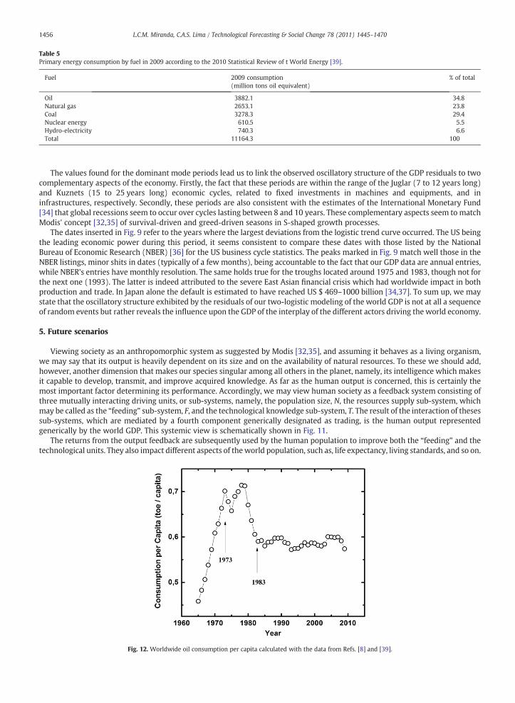
Table 5Primary energy consumption by fuel in 2009 according to the 2010 Statistical Review of t World Energy [39].

Fuel 2009 consumption(million tons oil equivalent)

% of total

Oil 3882.1 34.8Natural gas 2653.1 23.8Coal 3278.3 29.4Nuclear energy 610.5 5.5Hydro-electricity 740.3 6.6Total 11164.3 100

Fig. 12. Worldwide oil consumption per capita calculated with the data from Refs. [8] and [39].


The values found for the dominant mode periods lead us to link the observed oscillatory structure of the GDP residuals to twocomplementary aspects of the economy. Firstly, the fact that these periods are within the range of the Juglar (7 to 12 years long)and Kuznets (15 to 25 years long) economic cycles, related to fixed investments in machines and equipments, and ininfrastructures, respectively. Secondly, these periods are also consistent with the estimates of the International Monetary Fund[34] that global recessions seem to occur over cycles lasting between 8 and 10 years. These complementary aspects seem to matchModis' concept [32,35] of survival-driven and greed-driven seasons in S-shaped growth processes.

The dates inserted in Fig. 9 refer to the years where the largest deviations from the logistic trend curve occurred. The US beingthe leading economic power during this period, it seems consistent to compare these dates with those listed by the NationalBureau of Economic Research (NBER) [36] for the US business cycle statistics. The peaks marked in Fig. 9 match well those in theNBER listings, minor shits in dates (typically of a few months), being accountable to the fact that our GDP data are annual entries,while NBER's entries have monthly resolution. The same holds true for the troughs located around 1975 and 1983, though not forthe next one (1993). The latter is indeed attributed to the severe East Asian financial crisis which had worldwide impact in bothproduction and trade. In Japan alone the default is estimated to have reached US $ 469–1000 billion [34,37]. To sum up, we maystate that the oscillatory structure exhibited by the residuals of our two-logistic modeling of the world GDP is not at all a sequenceof random events but rather reveals the influence upon the GDP of the interplay of the different actors driving the world economy.

5. Future scenarios

Viewing society as an anthropomorphic system as suggested by Modis [32,35], and assuming it behaves as a living organism,we may say that its output is heavily dependent on its size and on the availability of natural resources. To these we should add,however, another dimension that makes our species singular among all others in the planet, namely, its intelligence which makesit capable to develop, transmit, and improve acquired knowledge. As far as the human output is concerned, this is certainly themost important factor determining its performance. Accordingly, we may view human society as a feedback system consisting ofthree mutually interacting driving units, or sub-systems, namely, the population size, N, the resources supply sub-system, whichmay be called as the “feeding” sub-system, F, and the technological knowledge sub-system, T. The result of the interaction of thesessub-systems, which are mediated by a fourth component generically designated as trading, is the human output representedgenerically by the world GDP. This systemic view is schematically shown in Fig. 11.

The returns from the output feedback are subsequently used by the human population to improve both the “feeding” and thetechnological units. They also impact different aspects of theworld population, such as, life expectancy, living standards, and so on.

image of Fig.�12

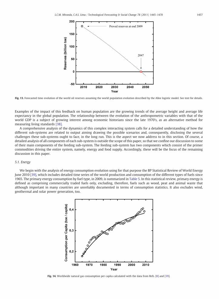
Fig. 13. Forecasted time evolution of the world oil reserves assuming the world population evolution described by the Allee logistic model. See text for details

Fig. 14. Worldwide natural gas consumption per capita calculated with the data from Refs. [8] and [39].


.

Examples of the impact of this feedback on human population are the growing trends of the average height and average lifeexpectancy in the global population. The relationship between the evolution of the anthropometric variables with that of theworld GDP is a subject of growing interest among economic historians since the late 1970's, as an alternative method formeasuring living standards [38].

A comprehensive analysis of the dynamics of this complex interacting system calls for a detailed understanding of how thedifferent sub-systems are related to output aiming drawing the possible scenarios and, consequently, disclosing the severalchallenges these sub-systems ought to face, in the long run. This is the aspect we now address to in this section. Of course, adetailed analysis of all components of each sub-system is outside the scope of this paper, so that we confine our discussion to someof their main components of the feeding sub-system. The feeding sub-system has two components which consist of the primercommodities driving the entire system, namely, energy and food supply. Accordingly, these will be the focus of the remainingdiscussion in this paper.

5.1. Energy

We begin with the analysis of energy consumption evolution using for that purpose the BP Statistical Review of World EnergyJune 2010 [39], which includes detailed time series of the world production and consumption of the different types of fuels since1965. The primary energy consumption by fuel type, in 2009, is summarized in Table 5. In this statistical review, primary energy isdefined as comprising commercially traded fuels only, excluding, therefore, fuels such as wood, peat and animal waste thatalthough important in many countries are unreliably documented in terms of consumption statistics. It also excludes wind,geothermal and solar power generation, too.

image of Fig.�13

image of Fig.�14

Fig. 15. Natural gas consumption as modeled by a bounded exponential growth as described by Eq. (15) of the text. The inset depicts the situation up to our days

Fig. 16. Forecasted time evolution of the world natural gas reserves assuming the world population to evolve according to our Allee logistic model. See text fordetails.


.

As a complement to Table 5 we add that by the end of 2009 the proved oil and gas reserves amounted to 181.8 billion of tons oilequivalent (toe) for oil, and 168.7 billion toe for natural gas. Table 5 tells us that roughly 88% of the world primary energyconsumption is due to fossil fuels, with oil and gas accounting for approximately 59% of the total. It seems, therefore, reasonable tofocus on these two types of fuels when providing a first account of the energy consumption evolution. Using the BP data on the oilyearly consumption aswell as the correspondingworld population data fromMaddison data base [8] we have construed the yearlyoil consumption per capita data, which is graphically displayed in Fig. 12.

Fig. 12 shows that between 1965 and 1973 the per capita oil consumption increased in a somewhat linear fashion. From 1973,as a result of the oil crisis it initially oscillated during the following 6 years to finally stabilize from 1983 on at an average per capitaconsumption of the order of 0.6 toe/people. Using our ALM estimate of the world population evolution and assuming that the oilper capita consumption remains stable at the rate of 0.6 toe/people we can calculate the future evolution of the oil reserves. Theresult is shown in Fig. 13.

Fig. 13 indicates that by 2047–48 the world proved oil reserves, as reported in the BP world energy review, should come to anend. We shall postpone the discussion of the impacts of this forecasting to the end of this section. Meanwhile, we move to theanalysis of the gas consumption data.

Following the same procedure as above, we show in Fig. 14 the evolution of the world per capita gas consumption from 1965 to2009.

As opposed to the case of oil, the evolution of the per capita natural gas consumption, shown in Fig. 14, can be seen as havingnot yet reached a reasonably stable plateau over the last 26 years. This is probably due to the fact that, being a relatively newlyexplored energy source, in comparison to oil, it has not yet reached a worldwide as intensive use as oil, a more than a century oldenergy source. In fact, Fig. 14 shows that the gas per capita consumption is still a growing function of time. The time evolution of

image of Fig.�15

image of Fig.�16

Table 6Values of some relevant indicators regarding the food balance and utilization of four major aggregate food groups taken from Ref. [40].

Item Food fraction Per capita food supply Total production

kg/capita/yr billion tons

1961 2007 1961 2007 1961 2007

Cereals 0.49 0.46 127.8 147 0.79 2.12Starchy roots 0.54 0.57 79.9 62 0.45 0.71Meat 0.99 0.98 23 40 0.07 0.27Milk 0.67 0.83 75.1 85 0.34 0.68

Fig. 17. Evolution of the per capita cereal supply since 1960. The solid line represents the time evolution modeling assuming a bounded exponential growth of thetype given by Eq. (15).


the per capita gas consumption was, accordingly, modeled assuming a bounded exponential growth. The corresponding datafitting yielded:

0:178 + 0:248 1−e− t−1965ð Þ=25:02Þh ið15Þ

ented in Fig. 14 by the solid line curve. Uponmultiplying Eq. (15) by our ALM estimate for theworld population we can then
represcalculate the time evolution of the world gas consumption. This is displayed in Fig. 15 by the solid line.
Knowing the gas consumption as a function of time the evolution of the natural gas reserves is readily obtained, as displayed inFig. 16.

From the above results we conclude the current world proven gas reserves, as reported in the BP world energy review, shouldlast about 10 years after the oil reserves have been depleted.

5.2. Food supply

The analysis of the future scenarios of food supply were based on FAO's Supply Utilization Accounts and Food Balance Sheets[40], last updated on June 02, 2010. The Food Balance Sheets, spanning from 1961 to 2007, provide detailed accounts of the majorcrops, livestock and fish production, including the corresponding fractions that are used as feeding (when applicable), as seed, aswell as the fraction that goes to industrial processing andwaste, and the fraction that is ultimately used as food. In this analysis wefocused our attention on the time evolution of fourmajor aggregate food groups, namely, cereals, starchy roots, meat andmilk. Thedata regarding the evolution of some relevant indicators of these items are summarized in Table 6.

The aggregate cereal group is by far the one that makes the most extensive use of land, water, fertilizers and energy, apart fromentering in the production chain of some other items, as, for instance, in the feeding of most livestock. In this regard it may beconsidered as the master agro-commodity. Accordingly, we shall confine the present discussion to the detailed analysis of thefuture trend and demand of this special group of food.We remark, however, that the overall conclusions we reached regarding thefuture supply and demand for the cereal group are equally applicable to the other three groups listed in Table 6.

In Fig. 17 we show the evolution of the per capita cereal supply from 1961 to 2007. From 1980 onwards, the data suggests adistinctively clear tendency towards saturation at an average per capita cereal supply of the order of 149 kg/capita/year.

On the other hand, if one models the time evolution of the per capita cereal supply data displayed in Fig. 17 assuming abounded exponential growth, similar to the one used in the previous case of the per capita gas consumption as given by Eq. (15),

image of Fig.�17

Fig. 18. Evolution of the worldwide cereal harvested area and yield according to FAO's latest report [40].

Fig. 19. Fluctuations of the cereal harvested area with respect to its average value. The solid line represents the fluctuations reconstruction using a truncated sineseries approach as discussed in the text. The amplitudes of the harmonic modes are displayed in the inset.


one finds a saturation value for per capita cereal supply of about 152 kg/capita/year. Thus, taking that figure for a guide, andassuming that the per capita cereal supply remains constant over the next years at an average value of 150 kg/capita/year, andconsidering our previous forecast that the world population by 2050 will be 8.9 billion people, we estimate that by the middle ofthe 21st century the cereal food supply needed to meet the human population demand at the same levels as in 2009 will be of theorder of 1.34 billion tons. Now, noting from Table 6 that the cereal fraction that is used as food correspond to roughly 0.46 of thetotal cereal production, we then forecast that an overall cereal production of about 2.9 billion tons will be needed to keep theworld population fed at the same patterns as the present ones.

To answer the question whether supplying this required cereal production is feasible or not, one has to estimate what shouldbe the size of the planted area needed for that. To that purpose let us consider the FAO's data on the cereal harvested area and yield.In Fig. 18 we plot the evolution of these two parameters from 1961 to 2009.

Fig. 18 indicates that over the last 48 years the cereal harvested area remained practically constant at around6.9±0.2 million km2,while the yield has increased linearly at a rate of about 0.044 tons/ha/year. Froma conservative standpoint, assuming that in the futuretherewill beno further gains in cereal yields, remainingpractically constantat the sameaverage observed for the last 10 years, namely,of theorder of 3.3 tons/ha/year,we estimate thatby2050weshall needanoverall cereal planted area in 2050of nearly 8.8 million km2

in order to achieve the goal of a total cereal production of about 2.9 billion tons in that year. This means that an additional1.8 million km2 of cereal planted areawill have to be added into the cereal production system in the next 41 years, should the annualcrop yield remain unchanged.

Even though this amounts to quite a large area, it can easily be fulfilled by incorporating new promising areas into production.For instance, the African tropical savanna [41,42] could be a possibility, for it presents similar soil and climate characteristics asthose of the Brazilian savannas, which are the most productive grain producing areas in that country. Thus, on considering thispossibility as a scenario for forecasting, then with the current technology for grain production that has been used in that Brazilianbiome, the incorporation of some 20 to 25% of the African savanna would add some 1.5 million km2 and thereby closely meet the

image of Fig.�18

image of Fig.�19


needs. That is, a feasible solution to meet the previously forecasted demand for grain production with the expansion of theagricultural area could be the one pointed out by this scenario, the difficulties for its implementation being much more of apolitical nature than due to some physical or technical barriers.

A second, more optimistic scenario may be considered with its forecasting based upon the assumption that, during the next40 years or so, the crop yield trend will keep on its so far linear growth path (see Fig. 18). In this case, we may expect that by 2050the cereal yield will of about 5 tons/ha/year. The cereal planted area, needed to achieve the prospective demand for 2.9 billion tonsof overall cereal production, would then be of the order of only 5.7 million km2. In other words, under this optimistic scenario, thecereal planted area needed would be reduced to some 81% of the currently planted 7 million km2. This forecasting may in fact beviewed as the more realistic one. The fast growth of the different biotechnologies as well as in the new field of synthetic biologyopens new, so far unforeseen, scenarios that may radically change life and production patterns in the near future. In fact, theBrazilian Agricultural Research Corporation estimates that if all grain producing farmers in that country make use of their alreadycurrently available technology, the grain yield could be increased by 50%, reaching thereby something of the order of 4.5 tons/ha/year without adding a single acre to the planted area. We shall postpone to the next section the discussion of some more criticalissues regarding the future food supply scenarios.

We conclude this discussion on the time evolution of the cereal food supply with a brief analysis of the cereal harvested areafluctuations with respect to its average value. In Fig. 19 we plot the fluctuations of the world cereal planted area with respect to itsaverage value. The solid line in this figure represents the fluctuations reconstruction using the same truncated sine series approachas we have done in the previous section, namely, by fitting the fluctuations to Eq. (14).

The results of the cereal planted area fluctuations data fitting to Eq. (14) yielded a fundamental frequency corresponding to aperiod of 55.4 years. The dominant modes, in decreasing order of amplitudes, were the first, second, fourth, third and fiftyharmonics, the corresponding periods being 55.4, 27.7, 13.9, 18.5, and 11.1 years. The amplitudes of these dominant modes areshown in the inset in Fig. 19. These dominant modes periods match well with those of the major economical cycles, namely, theJuglar cycles, from 7 to 11 years long, related to fixed investments in machines and equipments, the Kuznets cycles, related toinvestments in infrastructure, of endurance of 15 to 25 years, and the long Kondratiev cycles, from 45 to 60 years, related to thecritical transformation of the global macro-economy. Their appearance in the time evolution of major agricultural commoditiesindicators comes in, in our view, as no surprise at all, given their paramount economic importance.

6. Discussion

We begin addressing the food supply subject. The first aspect to be emphasized here is that the forecasts regarding the foodsupply, presented in the previous section, are essentially underestimates, since they assume that the current patterns of grainproduction and use remain unaltered for the next 40 years, e.g. that no further increase on the use of grains to produce fuel occurs.Under these circumstances it was emphasized that we still have plenty of room to expand grain production for food consumption,provided adequate new policies and political actions, on a global scale, be seriously considered. The critical threats to thefulfillment of the prospective grain-for-food demands are the increasing current tendency of using grains for fuel production, theeventual climate change impacts on crops yields, and an eventual population growth upsurge.

In a recent article, Lester Brown [43] presents an update discussion on future food shortage and the decision on reducing oilinsecurity by converting grain into fuel for cars. The food price inflation resulting from this decision is being felt all over the world.In some industrialized countries this ranges from 12 to 20% of food price increase, and in Mexico, corn meal prices went 60%higher. However, the most dramatic impact of this food price inflation is for those living on lower end of the global economyladder. As noted by Brown [43], referring toWorld Bank reports, each 1% rise in food prices produces a caloric intake drop of about0.5% among the poor people. No doubt that searching for green fuels, which means using both renewable and less-pollutingbiofuels and fuel cells, and developing new means of more efficient transportation is a priority. However, the point to be stressedhere is that there is no real need to base biofuels production upon grains at the expense of jeopardizing grain-to-food production,as worldwide experience has shown.

Besides the foregoing issues, probably the most difficult and challenging threat to be dealt with in designing an adequateframing for the sustainable and affordable food supply regards the climate change issue. This discussion has acquired in recentyears a passionate character due to the many conflicting interests that are inevitably involved. The whole issue of the impacts ofclimate changes in the agricultural production is still quite controversial. One of themost frequently used arguments, so far, is thatclimate changeswill have a substantial impact on the agriculture in tropical and sub-tropical regions of the globe.We shall perhapsadd an extra bit of controversy to this argument on disclosing in what follows the results of our analysis about the Brazilian grainproduction experience in this particular regard.

Table 7Brazilian average soybean productivity between 2004 and 2008 at different latitudes.

Latitude interval Average productivity (kg/ha) Mean annual temperature (°C)

0°–13° S 2750 Above 25 °C15°–23° S 2602 Between 20°–25 °C25–33° S 2252 Below 20 °C

Fig. 20. Time evolution of the per capita total primary energy consumption. The solid gray line represents the data modeling to a bounded exponential growthwhereas the black line shows the approximate linear growth up to 1973.


,

As a result of heavy investments in agricultural R&D this country was able to develop new varieties of soybeans (a typicaltemperate climate grain species), adapted to different soils and to both thermal and water stress conditions, to become a majorplayer in the production of this grain. Originally, Brazilian soybeans plantations were located only in the southern states belowlatitudes of about 25° S. Nowadays, they can be found over practically all regions of this country, from the Equator down tolatitudes of about 33° S. We have collected soybean productivity data at different regions of this country. They are summarized inTable 7 giving the average soybean productivity between 2004 and 2008, as a function the latitude for themain producing regions.

Table 7 shows that, provided the properly adapted varieties are selected for planting, the productivity does in fact increase aswemove up towards the tropical areas.We also note that the average temperature excursion between these three latitude strata isof about 5°C, which happens to be the maximum temperature rise predicted by the different global warming models in use. Thisexample shows that on evaluating the impacts of climate changes on agro-production one should definitely not neglect, in makingforecasts, the counter-action associated to the intangible components deriving from technology intelligence.

No matter which solution is adopted for the future supply of a given commodity, its success will ultimately depend onwarranting adequate supply of the master commodity, i.e., energy. The energy security issue is certainly the most challengingproblem one will face in the near future. Even though other existing oil and gas reserves estimates may differ from the ones wehave used in this work, the point is that inevitably these fossil fuel sources will certainly have to be replaced by others still duringthis century. As seen in the previous section, oil and gas account for roughly 60% of the world total primary energy consumption(PEC). The inevitable depletion of these sources will definitely promote an eventual radical change in the current PEC profile.

In Fig. 20 we show the time evolution of the per capita total primary energy consumption. Up to 1973 the PEC exhibits a lineargrowth but from then on the slope gradually decreases in time in a way that suggests a tendency towards a plateau.

Modeling the time evolution of the PEC data shown in Fig. 20 by a bounded exponential growth of the type given by Eq. (15) onefinds a saturationof the per capita primary energy consumption at about 1.57 toe/people. On takingour previously forecastedworldpopulation for 2050 of 8.9 billion peoplewe estimate at 14 billion toe the total primary energy consumption demand by themiddleof the century. This corresponds to an increase of the order of the 3 billion toe over the current (2009) PEC of 11 billion toe (c.f.,Table 5). This means that during the next 40 years, or so, the primary energy production will have to increase at a yearly rate ofaround 0.6% in order to meet the forecasted demand. This amounts to be adding, on the average, something of the order of75 million toe to the primary energymatrix each year, for the next 40 years. To give an idea of how large such an annual increase inthe PEC is, it comes out to be equivalent to the 2009 nuclear energy consumption of both Japan (62 million toe) and Spain(12 million toe) taken together.

On considering large scale production, it is clear that one immediate, technologically available, energy source capable toreplacing oil and gaswould be nuclear energy. Nuclear energy is amature, safe and reliable technology capable of supplying energyon a large scale, at an affordable price, and without pollution or greenhouse gasses. Because of these virtues, and the technology'sability to confer greater energy independence, governments around the world have increasingly considered nuclear power as anoption in their energy matrix plans for the future. For some countries it is a central element in their national energy strategies. Ofcourse, decision making towards its adoption will call for the strictest enforcement of new safety innovations that warrantprotection for the reactor and the full operating plant against both human errors and natural catastrophes disasters which, thoughrare, have produced dramatic events with worldwide impact and increased concern toward safer nuclear energy power plants.

The currently commercially available nuclear energy is baseduponuranium fuelednuclearfission reactors. That is, it depends ona finite source of fueling material, although the proved reserves of this material ensures some 100 years of adequate supply. Formany people, however, this is a rather controversial issue and for some a non-issue at all. In fact, like it happened in the recent pastin regards to fossil energy resources, where the prospects for source exhaustion kept on being reassessed and the proven reserveswere continuously pushed forward by orders of magnitude, as more oil and gas was found than was consumed, a similar trend has

image of Fig.�20


involved the assessment of nuclear energy resources, particularly uranium ore, for nuclear fuel. Some experts say that the currentproven reserves estimates are flawed for two primary reasons. Firstly not enough effort and money have backed up uranium oreexploration, including due to the fact that the nuclear energy use boomanticipated for the 1960–1970's did not come by, for severalreasons, and the resources that were being explored/mapped soon realized to be more than enough to fuel the demand ofworldwide nuclear reactors that came into operation to date. Secondly, these assessments neglect in their accounting the almostinexpressive effect that the price of uraniumore has on thefinal nuclear power price (as opposite to the case of oil andgas in relationto fossil fuels power plants) and have accordingly set the maximum allowable prices, to determine economic returns, far too low.

Now in regards to fission energy reactors it is a fact that new nuclear energy technology prospects are being continuouslyadvanced, as to reactor safety, nuclear waste disposal, alternative nuclear fuels, and also in regards to fuel recycling, as in the socalled breeder reactor design. However, going into further details would be out of the scope of this paper. To close the foregoingremarks, we would like to quote a statement from the begin of the XXI century [44], in regards to fueling nuclear energy fissionreactors: Availability of Ore — Sustainability Potential: “For such recycle based fuel cycles, if exploited fully, at least a millennium ofenergy supply can be foreseen from the earth's endowment of economically recoverable uranium ore .... Likewise, the energy potential ofthe earth's endowment of thorium is greater still. Thus the resource base is sufficient to support the sustainability goal — given that thefuel cycles and reactor types are deployed to fully exploit those resources.”

The alternative to the nuclear fission technology is the nuclear fusion with a considerable number of advantages over fissiontechnology. Firstly, the energy released in nuclear fusion processes is three to four times greater than that release in fissionreactions. Secondly, nuclear fusion creates less radioactive material than fission and its fuel supply (e.g., hydrogen) is practicallyunlimited. For these reasons during the 1970's, just after the 1973 oil crisis, there were government efforts to invest in thedevelopment of the controlled nuclear fusion technology. These efforts were soon to bemostly relegated to university laboratoriespilot experimental researches due to a draw back in the scaling up of this technology, namely, the energy required to bring two ormore protons close enough so that nuclear forces overcome their electrostatic repulsion and trigger the fusion reaction isextremely high. Nevertheless, it seems clear that new efforts towards the development of alternative nuclear fusion technologiesought to be strengthened along this century if mankind aims a permanent, practically unlimited, energy supply in the future. Thisendeavor, involving large capital investments, as well as sensible security issues, should probably be conducted under globalgovernance and partnership.

As amatter of fact, a pioneer pilot effort in this direction, is already underway, in Cadarache, France, aiming atmaking it feasibleto bring fusion energy into the commercial market, and joining in an unprecedented € 5 billion (may end up reaching € 15 billion)collaboration involving China, the European Union, India, Japan, Korea, Russia and the United States who funded andmanpoweredwith their scientists and technicians the International Thermonuclear Experimental Reactor (the ITER). It is currently the world'slargest and most advanced experimental tokamak nuclear fusion reactor facility, designed to produce 500 MW of output powerfrom 50 MW of input power, that is to say, ten times the amount of energy put in.

However, any political and economic solutions are always accompanied by positive and negative externalities. In the case of thenuclear energy, in addition to the well known environmental hazards, there are also important political and security concerns,regarding the potential proliferation use of this sensible technology, especially in an era of growing terrorism. But, this is certainlyan unavoidable issue that the world leaders have to consider when negotiating a compromise solution. The post WorldWar II era,characterized as a period of unprecedented economic boom driven by the fast growth of new technologies, induced the leadingnations to adopt measures to control the proliferation of mass destruction weapon technologies, since the 1950's. However,despite these non-proliferation measures, international and intra-national conflicts kept increasing considerably not only in thefrequency of events but also in their severities, a situation that has prompted a remark by Linstone [45], “the lessons that can belearned from the non-proliferation efforts are hardly encouraging”. Another conflicting aspect regarding the non-proliferation actionsis that it is usually accompanied by measures which restrict the knowledge diffusion, and, consequently, slow down the diffusionof the frontiers of science and technology worldwide. Non-proliferation sanctions may eventually stay effective only to a limitedtime scale.

Finally, another important and sensible aspect that most certainly will influence the outcome of the forecasted scenariosdiscussed in this paper regards the world political leadership issue. As noted by Kennedy [46], “the relative strengths of the leading

Table 8Top 10 most indebted countries ordered according to debt in decreasing percentage of its GDP.

Country External debttrillion 2009 US $

% GDP Forex reservestrillion 2010 US $

Debt/Forex Resources Labor

Natural Intellectual

Luxembourg 1.994 3854% 0.0008 2492.50 Low Moderate LowIreland 2.287 1004% 0.002 1143.50 Low High LowNetherlands 3.733 470% 0.038 98.24 Low High LowUnited Kingdom 9.088 416% 0.097 93.69 Low High ModerateHong Kong 0.655 311% 0.261 2.51 Low High LowSwitzerland 1.339 271% 0.256 5.23 Low High LowBelgium 1.354 267% 0.025 54.16 Low High LowPortugal 0.507 223% 0.018 28.17 Low Moderate LowAustria 0.809 212% 0.019 42.58 Low High LowDenmark 0.607 196% 0.073 8.32 Low High Low

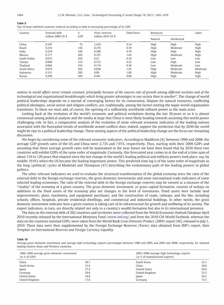
Table 9Top 10 least indebted countries ordered according to debt in increasing percentage of its GDP.

Country External debttrillion 2009 US $

%GDP

Forex reservestrillion 2010 US $

Debt/Forex Resources Labor

Natural Intellectual

China 0.347 7% 2.454 0.14 High High HighBrazil 0.216 14% 0.276 0.78 High Moderate HighIndia 0.224 18% 0.288 0.78 High High HighMexico 0.177 20% 0.107 1.65 High Moderate HighSaudi Arabia 0.072 20% 0.41 0.18 Low Low LowTaiwan 0.080 21% 0.372 0.22 Low High LowThailand 0.066 25% 0.174 0.38 Low Moderate LowSouth Africa 0.074 26% 0.038 1.95 High Moderate ModerateIndonesia 0.151 28% 0.08 1.89 High Moderate HighRussia 0.369 30% 0.461 0.80 High High High

Table 10Average gross domestic investment and average high technology exports percentages between 1980 and 2005 and 2005 and 2008, respectively, for selectedleading Eastern Asian and Western countries.

1980–2009 average gross domestic investment(as % of GDP)

2005–2008 average high technology exports(as % of manufactured exports)

China 38.7 South Korea 32.3South Korea 31.8 China 30.0Japan 27.4 United States 29.0Germany 20.8 United Kingdom 25.3United States 18.8 Japan 20.3United Kingdom 17.6 Germany 15.5


nations in world affairs never remain constant, principally because of the uneven rate of growth among different societies and of thetechnological and organizational breakthroughs which bring greater advantages to one society than to another”. The change of worldpolitical leaderships depends on a myriad of converging factors for its consecution. Dispute for natural resources, conflictingpolitical ideologies, social unrest and religion conflicts, are, traditionally, among the factors nesting the major world organizationtransitions. To these we must add, of course, the uprising of a sufficiently worldwide influent power as the main actor.

Looking back at the evolution of the world's economic and political evolutions during the last 30 years or so it is almostconsensual among political analysts and the media at large that China is most likely heading towards assuming this world powerchallenging role. In fact, a comparative analysis of the evolution of some relevant economic indicators of the leading nationsassociated with the forecasted trends of worldwide armed conflicts does, indeed, support the prediction that by 2030 the worldmight be ripe to a political leadership change. These nesting aspects of the political leadership change are the focus our remainingdiscussion.

We begin by considering some of the relevant economic indicators. According to Maddison [8], between 1990 and 2008, theaverage GDP growth rates of the US and China were 2.73% and 7.97%, respectively. Thus, starting with their 2009 GDPs andassuming that these average growth rates will be maintained in the near future we have then found that by 2030 these twocountries will exhibit GDPs of the same order of magnitude. Curiously, this forecasted year comes in at the end of a time span ofabout 110 to 120 years that elapsed since the last change in the world's leading political and military powers took place, say, bymiddle 1910's when the US became the leading hegemonic power. This predicted time lag is of the same order of magnitude asthe long (political) cycles of Modelski and Thompson [47] describing the evolutionary path of the leading powers in globalpolitics.

The other relevant indicators we used to evaluate the structural transformation of the global economy were the ratio of theexternal debt to the foreign exchange reserves, the gross domestic investments and some international trade indicators of someselected leading economies. The ratio of the external debt to the foreign exchange reserves may be viewed as a measure of the“vitality” of the economy of a given country. The gross domestic investment, or gross capital formation, consists of outlays onadditions to the fixed assets of the economy plus net changes in the level of inventories. Fixed assets here include landimprovements; plant, machinery, and equipment purchases; and the construction of roads, railways, and the like, includingschools, offices, hospitals, private residential dwellings, and commercial and industrial buildings. In other words, the grossdomestic investment indicates how a given country is taking care of its infrastructure for growth and wellbeing of its society. Theexport indicators, in turn, are directly related not only to a country's wealth formation but also to its international presence.

The data on the external debt of 202 countries and territories were collected from theWorld Economic Outlook Database April2010 recently released by the International Monetary Fund (www.imf.org) and from the 2010 CIA World Factbook, whereas thedata on the countries nominal GDPs, were taken from theWorld Bank Gross Domestic Product (2009) report [48], released in July 1,2010. These data were then supplemented by the Foreign Exchange Reserves (Forex) data obtained from IMF's report, DataTemplate on International Reserves and Foreign Currency Liquidity.

http://www.imf.org

Fig. 21. Time evolution of the merchandise export shares of the world total of some selected Eastern Asian and Western countries.


The total external debt of the 202 countries and territories adds, by the end of 2009, to 61,796 trillion in 2009 US dollars. Theexternal debt of the top 50 most indebted countries is equal to 60,507 trillions 2009 US dollars, corresponding to 98.08% of thetotal external debt in the world at the end of 2009. In the Appendix we detail the full listing of these 50 most indebted countries,whereas in Tables 8 and 9 below we list the top 10 most and least indebted countries, respectively. As can be seen from Tables 8and 9 no matter which criterion one uses the group of the ten least indebted countries, consisting predominantly of Asiancountries and led by China, seems to be the one with greater potential to leading the future world economy.

In Table 10we summarized theWorld Bank data on the gross domestic investment (as percentage of GDP) and high technologyexports (as percentage of the total manufactures exports) of some selected leading Eastern Asia (China, S. Korea and Japan) andWestern (USA, UK, and Germany) countries. The high-technology exports refer to products with high R&D intensity, such as inaerospace, computers, pharmaceuticals, scientific instruments, and electrical machinery. The data listed in Table 10 refer to theaverage gross domestic investment and the average high technology exports percentages in the 1980 to 2009 and 2005 to 2008periods, respectively. In both cases the Eastern Asian countries lead the ranking.

The Chinese gross domestic investment evolved from 35% of its GDP in 1980 to 48% in 2009, whereas during the same periodthe US gross domestic investment decreased from 20% of its GDP to 14%. Using the 2009 World Bank GDP data for both countrieswe find that the gross capital formation in 2009 amounted to 2.39 trillion dollars, in China, against 1.96 trillion dollars in theUnited States. Even though the infrastructure discrepancy between the two countries is quite large, these figures indicate thetremendous effort China has undertaken to place the country in the economic leadership.

A somewhat similar situation is also evident in a comparative analysis of the total merchandise exports performance betweenthe selected Eastern Asian and Western countries. In Fig. 21 we show the combined merchandise exports shares of the EasternAsian and Western countries as shares of the world total. The data used in this plot were taken from the latest World TradeOrganization report [33]. The solid lines in these plots correspond to a single logistic growth function fit to the Eastern Asiancountries and a single logistic decay function fit to theWestern countries. The inflection points in these two plots are located in theyears 1977.1 and 2005.4 for the Eastern Asian andWestern countries, respectively. The extrapolations of the fitted curves indicatethat by 2031 the shares of these combined merchandise exports are expected to reach the same level.

Fig. 22. Evolution of the US and Chinese shares of the world's manufactures exports from 1980 through 2009.

image of Fig.�21

image of Fig.�22

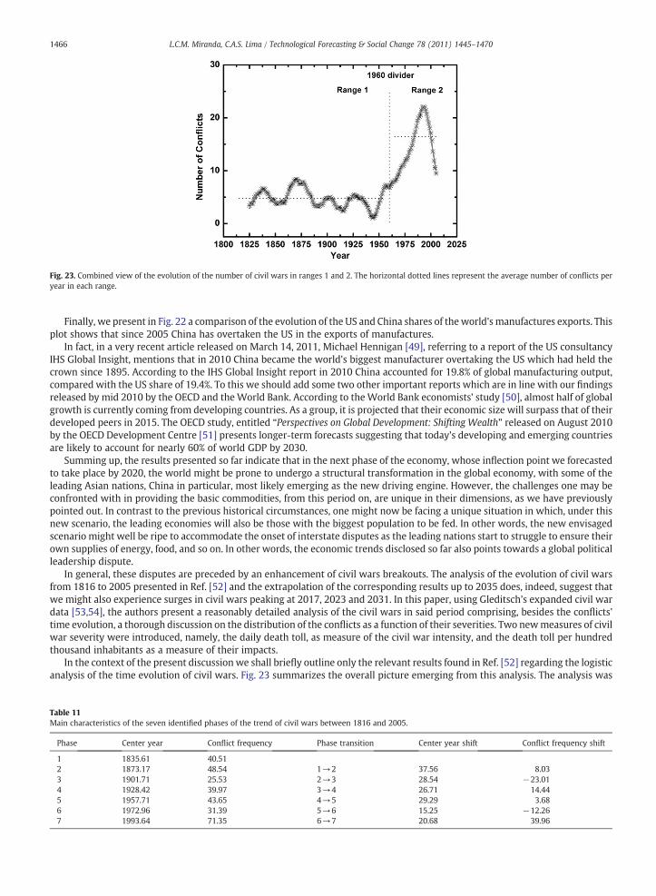
Fig. 23. Combined view of the evolution of the number of civil wars in ranges 1 and 2. The horizontal dotted lines represent the average number of conflicts peryear in each range.


Finally, we present in Fig. 22 a comparison of the evolution of the US and China shares of theworld's manufactures exports. Thisplot shows that since 2005 China has overtaken the US in the exports of manufactures.

In fact, in a very recent article released on March 14, 2011, Michael Hennigan [49], referring to a report of the US consultancyIHS Global Insight, mentions that in 2010 China became the world's biggest manufacturer overtaking the US which had held thecrown since 1895. According to the IHS Global Insight report in 2010 China accounted for 19.8% of global manufacturing output,compared with the US share of 19.4%. To this we should add some two other important reports which are in line with our findingsreleased by mid 2010 by the OECD and theWorld Bank. According to theWorld Bank economists' study [50], almost half of globalgrowth is currently coming from developing countries. As a group, it is projected that their economic size will surpass that of theirdeveloped peers in 2015. The OECD study, entitled “Perspectives on Global Development: Shifting Wealth” released on August 2010by the OECD Development Centre [51] presents longer-term forecasts suggesting that today's developing and emerging countriesare likely to account for nearly 60% of world GDP by 2030.

Summing up, the results presented so far indicate that in the next phase of the economy, whose inflection point we forecastedto take place by 2020, the world might be prone to undergo a structural transformation in the global economy, with some of theleading Asian nations, China in particular, most likely emerging as the new driving engine. However, the challenges one may beconfronted with in providing the basic commodities, from this period on, are unique in their dimensions, as we have previouslypointed out. In contrast to the previous historical circumstances, one might now be facing a unique situation in which, under thisnew scenario, the leading economies will also be those with the biggest population to be fed. In other words, the new envisagedscenario might well be ripe to accommodate the onset of interstate disputes as the leading nations start to struggle to ensure theirown supplies of energy, food, and so on. In other words, the economic trends disclosed so far also points towards a global politicalleadership dispute.

In general, these disputes are preceded by an enhancement of civil wars breakouts. The analysis of the evolution of civil warsfrom 1816 to 2005 presented in Ref. [52] and the extrapolation of the corresponding results up to 2035 does, indeed, suggest thatwe might also experience surges in civil wars peaking at 2017, 2023 and 2031. In this paper, using Gleditsch's expanded civil wardata [53,54], the authors present a reasonably detailed analysis of the civil wars in said period comprising, besides the conflicts'time evolution, a thorough discussion on the distribution of the conflicts as a function of their severities. Two newmeasures of civilwar severity were introduced, namely, the daily death toll, as measure of the civil war intensity, and the death toll per hundredthousand inhabitants as a measure of their impacts.

In the context of the present discussion we shall briefly outline only the relevant results found in Ref. [52] regarding the logisticanalysis of the time evolution of civil wars. Fig. 23 summarizes the overall picture emerging from this analysis. The analysis was

Table 11Main characteristics of the seven identified phases of the trend of civil wars between 1816 and 2005.

Phase Center year Conflict frequency Phase transition Center year shift Conflict frequency shift

1 1835.61 40.512 1873.17 48.54 1→2 37.56 8.033 1901.71 25.53 2→3 28.54 −23.014 1928.42 39.97 3→4 26.71 14.445 1957.71 43.65 4→5 29.29 3.686 1972.96 31.39 5→6 15.25 −12.267 1993.64 71.35 6→7 20.68 39.96

image of Fig.�23

Fig. 24. Residuals from the five logistic pulses modeling of the time evolution of civil wars in range 1. The solid line represents the results of a truncated sine seriereconstruction.

Fig. 25. Residuals from the five logistic pulses modeling of the time evolution of civil wars in range 2. The solid line represents the results of a truncated sine seriereconstruction.


s

carried out using a multi-logistic modeling of the civil wars chronology in the two markedly distinct time ranges: a first rangebetween 1816 and the beginning of 1960 decade, and a second one from 1960 to 2005. These ranges are denoted as ranges 1 (1816to 1960) and 2 (1960 to 2005). Range 1 comprised five logistic phases centered around 1836, 1873, 1902, 1928, and 1958, whilerange 2 consisted of two main logistic phases centered about 1972 and 1993. The horizontal dotted lines represent the averagenumber of conflicts per year in ranges 1 and 2, respectively, while the solid line describes the number of conflicts as obtained fromthe logisticmodeling. It was found that the average peak-to-peak time span is of the order of 26.3 years, thereby indicating that theworld has experienced a peak in the number of conflicts every, say, 26 years.

Table 11 consolidates the main characteristics of the seven identified phases of the trend of civil wars between 1816 and 2005.It displays the center year of each phase, the average number of conflicts per year for each phase, the time lapse between the centeryears of consecutive phases (center year shift) and the difference between the average number of conflicts (conflict frequencyshift) for the sequential phases.

Fig. 23 and Table 11 indicate that frequencies of civil wars have considerably increased over the 20th century. Even though notshown here, the same is also true regarding the civil wars severity.

Other relevant aspects for our discussion are connected to the results found in Ref. [52] from the fine-coarsed analysis of thedata-tomodel residuals of the civil wars trend. The sine-series reconstruction of the residuals in ranges 1 and 2 are displayed inFigs. 24 and 25, respectively.

The residuals for range 1, besides the fundamental period of 27.8 years, display dominant harmonics corresponding to periodsof 13.9, 7.0 and 9.3 years. The corresponding results for range 2, for which the fundamental period was found to be of 30.8 years,indicate that the dominant period (namely, 7.7 years) is roughly half of that of range 1 (13.9 years). The interesting outcome in thecontext of the present paper regards the extrapolation of the residuals reconstruction in range 2 shown in Fig. 25. Thisextrapolation indicates that we might expect peaks in civil wars by 2017, 2023 and 2031.

s

image of Fig.�24

image of Fig.�25


In conclusion, we may say that not only the economic trends we have analyzed but also the social unrest as described by civilwar breakouts support the forecast that by the 2020s we might see a change of global economic and political leadership.

7. Conclusions

In this paper we have initially presented a comparative discussion between the logistic and power law methodologies foranalyzing long range time series of evolutionary growth of finite resources systems. Typical examples of these processes arethe evolution, over the Christian era, of the human population and its productive output as represented by its GDP. It wasshown that the power law modeling may provide a reasonable description only at the early stages of the process when thesystem is in a replication, or depensation, phase. As the system evolves in time and reaches some critical size its evolutionarygrowth tends to become a diffusion-reaction controlled process acquiring an S-shaped time dependence, which, in turn,entails that it may be described by conventional sigmoid functions, like the Verhulst logistic function. A generalization of theVerhulst logistic modeling to allow for the possibility of a nonlinear replication component of the growth process wasdescribed in Ref. [24]. This more general modeling of S-shaped processes was referred to in that paper as the Allee logisticmodel of evolutionary process.

The Allee logistic model was then applied to the evolution of the world GDP from 1 to 2008 AD. It was found that it ischaracterized by a broad phase centered on a world population of about 3.68 billion people (corresponding approximately to theyear 1970), and predicts a second phase to peak when the world population reaches a size around 7.51 (corresponding to the year2020). From then on the world GDP evolves towards approaching a saturation value of the order of 142 trillion internationaldollars, at a faster rate than that in previous phase. This forecasting of a second phase of economic growth agrees with twoindependent works, namely, that of Ayres [31] who predicts a peak of the 5th K-wave to occur by that year, as well as with that ofModis [32], who predicts an economic boom peaking at the mid-2020s based on his analysis of the historical data on energyconsumption. It was also shown that this new phase of economic growth is further supported by the analysis of the world tradeevolution. The recently released statistics on the international trade [33] shows that since 1955 the world trade exports value hasentered a phase of explosive growth as compared to the exports volume, leading us to infer that a corresponding higher increase inthe pace of aggregating value to products might be under way.

The analysis of the residuals of the Allee logistic modeling of the world GDP unveils that they are not a sequence of randomevents but rather that they exhibit a marked underlying oscillatory structure with periods that fall in the range corresponding tothose associated to both of Juglar and Kuznets economic cycles. The largest deviations from our logistic trend curve were alsofound to be in good agreement with the NBER's economic cycle statistics.

Next, we moved on to present a systemic view of human society as a feedback input–output system in which the output is theworld GDP and the input consists of three mutually interacting sub-systems, namely, the population size sub-system, the feedingsub-system (comprising all the resources supplies available), and the technological and social intelligence sub-systems(comprising the accumulated human knowledge, including all of its relevant sources such as science, technology and technique,economy, and so on). The overall carrier of the interactions among these sub-systems, and their communication with the output(the GDP), are the human trading activities.

In forecasting the world future scenarios, based on the previous results regarding the population and GDP time evolutions, wefocused mainly on what we deemed to be the primer commodities driving the whole system, to wit, energy and food supply. Twoimportant aspects came out of this analysis. The first one regards the strict constraints forecasted for both food and energy suppliesby the middle of this century. The second one refers to the social and political leadership and worldwide public policies changesthat may seemingly take place by the year 2030.

To insure the required food and energy supplies needed to sustain life under the current patterns, apart from adopting policiesminimizing the negative economic externalities and improving considerably the use of renewable energy sources, our discussionindicates that future of human society will be heavily dependent on the successful development of new, more efficient and safertechnologies, especially in the areas of synthetic biology and biotechnology as well as in nuclear and renewable energy generation.

The social and political leadership changes envisaged in our discussion were based upon the combined analysis of the currenttrends of the vitalities of the economies of the major players in the world scene as well as of the evolution of global social unrest asrepresented by civil war breakouts. It simply confirms the historical fact that the relative strengths of the leading nations neverremain constant. Coincidently, the forecasted time span of 110 to 120 years since the last change in the world's leading politicalpowers, that occurred by themiddle of the 1910's when the US became the leadingworld power, is of the same order of magnitudeas the long (political) cycles of Modelski and Thompson [47].

In conclusion, we may say that human society is getting through an absolutely new situation of delicate balance, as comparedto those of the previous centuries, in which the political decisions of a given country can no longer be takenwithout considering itsworldwide impact. This is the price globalization is charging upon us. In previous centuries the relative size of the resources incomparison to that of population was quite favorable to the former and the prevailing economic policy was geared into economicgrowth. The forecasting discussed in this paper points to a new, completely different scenario calling for a change of paradigm.Instead of the traditional, essentially unconditioned, economic growth focus, the new paradigm gearing the future world politicsshould be that of sustainability. Otherwise, in just one generation time ahead we should begin to face serious economical crisesand social struggles with unpredictable political consequences. Even though it may sound utopist, we believe this new paradigm,imposed onto us by the globalization, is the only rational way through which our species can be preserved.


Appendix

List of the fifty most indebted countries ordered according to the increasing share of the debt with respect to the GDP.

Country External debtin trillion 2009 US $

Percentage of GDP Forex reservestrillion 2009 US $

Debt/Forex

China 0.347 7% 2.454 0.14Brazil 0.216 14% 0.276 0.78Índia 0.224 18% 0.288 0.78Mexico 0.177 20% 0.107 1.65Saudi Arabia 0.072 20% 0.41 0.18Taiwan 0.080 21% 0.372 0.22Thailand 0.066 25% 0.174 0.38South Africa 0.074 26% 0.038 1.95Indonesia 0.151 28% 0.08 1.89Russia 0.369 30% 0.461 0.80Philippines 0.053 33% 0.052 1.02Argentina 0.109 35% 0.051 2.14Chile 0.061 38% 0.025 2.44Czech Republic 0.077 39% 0.037 2.08Korea, South 0.334 40% 0.29 1.15Japan 2.132 42% 1.05 2.03Israel 0.085 43% 0.063 1.35Turkey 0.274 45% 0.077 3.56Poland 0.201 47% 0.086 2.34New Zealand 0.059 50% 0.018 3.28Slovakia 0.052 55% 0.002 26.00United Arab Emirates 0.129 56% 0.045 2.87Romania 0.095 59% 0.044 2.16Canada 0.834 62% 0.055 15.16Qatar 0.063 75% N/A –

Kazakhstan 0.093 85% 0.028 3.32Hungary 0.117 90% 0.043 2.72Ukraine 0.104 90% 0.031 3.35Australia 0.920 92% 0.036 25.56United States 13.450 94% 0.129 104.26Croatia 0.059 94% 0.013 4.54Italy 2.328 101% 0.144 16.17Slovenia 0.055 112% 0.001 55.00Norway 0.548 143% 0.049 11.18Finland 0.365 153% 0.01 36.50Germany 5.208 155% 0.197 26.44Spain 2.410 165% 0.03 80.33Sweden 0.669 165% 0.047 14.23Greece 0.553 167% 0.005 110.60France 5.021 188% 0.143 35.11Denmark 0.607 196% 0.073 8.32Austria 0.809 212% 0.019 42.58Portugal 0.507 223% 0.018 28.17Belgium 1.354 267% 0.025 54.16Switzerland 1.339 271% 0.256 5.23Hong Kong 0.655 311% 0.261 2.51United Kingdom 9.088 416% 0.097 93.69Netherlands 3.733 470% 0.038 98.24Ireland 2.287 1004% 0.002 1143.50Luxembourg 1.994 3854% 0.0008 2492.50

References

[1] H. Kan, A.J. Wiener, The Year 2000, Hudson Institute Inc., New York, 1967 This text is freely available at the site of the Hudson Institute at the followingaddress: http://www.hudson.org/files/publications/kahn_yr2000.pdf.

[2] I. Wallerstein, The Modern World-System, Academic Press, New York, 1974.[3] G. Modelski, Principles of World Politics, Free Press publishers, New York, 1972.[4] A.G. Frank, World system in crisis, in: W.R. Thompson (Ed.), Contending Approaches to World System Analysis, Sage Publications, Beverly Hills, 1983,

pp. 27–42.[5] G. Modelski, R.A. Denemark (Eds.), World System History, EOLSS, Oxford, UK, 2009.[6] T. Jackson, Prosperity without Growth, Earthscan, London, UK, 2009.[7] P.J. Klenow, A. Rodriguez-Clare, Externalities and growth, in: P. Aghion, S.N. Durlauf (Eds.), Handbook of Economic Growth, Vol. 1A, Elsevier, Amsterdam,

2005, pp. 817–861.[8] A. Maddison, Historical Statistics for the World Economy 1–2008 ADavailable at, http://www.ggdc.net last accessed Aug 16 2010.[9] L.C.M. Miranda, C.A.S. Lima, On trends and rhythms in scientific and technological knowledge: a quantitative analysis, Int. J. Technol. Intell. Plann. 6 (1)

(2010) 76–109.[10] J. Fisher, R. Pry, A simple substitution model of technological change, Technol. Forecast. Soc. Change 3 (1971) 75–88.

http://www.hudson.org/files/publications/kahn_yr2000.pdf

http://www.ggdc.net


[11] C. Marchetti, Society as a learning system: discovery, invention and innovations cycles revisited, Technol. Forecast. Soc. Change 18 (1980) 257–282.[12] C. Marchetti, Fifty years pulsation in human affairs, Futures 17 (1986) 376–388.[13] B.J.L. Berry, A pacemaker for the long wave, Technol. Forecast. Soc. Change 63 (2000) 1–23.[14] B.J.L. Berry, Low-frequency waves of inflation and economic growth: digital spectral analysis, Technol. Forecast. Soc. Change 68 (2001) 63–73.[15] T. Modis, Conquering Uncertainty, McGraw-Hill, New York, 1998.[16] G.P. Boretos, The future of the global economy, Technol. Forecast. Soc. Change 76 (2009) 316–326.[17] T. Devezas, Crises, depressions and expansions: global analysis and secular trends, Technol. Forecast. Soc. Change 77 (2010) 739–761.[18] S.P. Kaptiza, The phenomenological theory of world population growth, Physics-Uspekhi 39 (1) (1996) 57–71.[19] A. Johansen, D. Sornette, Finite-time singularity in the dynamics of the world population, economic and financial indices, Physica A 294 (2001) 465–502.[20] M. Kremer, Population growth and technological change: one million B.C to 1990, Q. J. Econ 108 (1993) 681–716.[21] A. Korotayev, A. Malkov, D. Khaltourina, Introduction to Social Macrodynamics: Compact Macromodels of the World System Growth, URSS Publishers,

Moscow, 2006.[22] G. Modelski, T. Devezas, W.R. Thompson (Eds.), Globalization as Evolutionary Processes, Routledge, Abingdon, UK, 2008.[23] L.C.M. Miranda, C.A.S. Lima, A new methodology for the logistic analysis of evolutionary S-shaped processes: application to historical time series and

forecasting, Technol. Forecast. Soc. Change 77 (2010) 175–192.[24] L.C.M. Miranda, C.A.S. Lima, On the logistic modeling and forecasting of evolutionary processes: application to human population dynamics, Technol.

Forecast. Soc. Change 77 (2010) 699–711.[25] W.C. Allee, Animal Aggregations: A Study in General Sociology, University of Chicago Press, Chicago, 1931.[26] M.S. Fowler, G.D. Ruxton, Population dynamics consequences of Allee effect, J. Theor. Biol. 215 (2002) 39–46.[27] L.C.M.Miranda, C.A.S. Lima, On depensation effects in logistic modeling of evolutionary processes: the case of automobiles annual fleet evolution, accepted for

publication at Int. J. Technol. Intell. Plann. (in press).[28] H. von Foerster, P. Mora, L. Amiot, Doomsday: Friday, 13 November, A.D. 2006. At this date human population will approach infinity if it grows as it has in the

last two millennia, Science 132 (1960) 1291–1295.[29] US Census Bureau, International Data Base, http://census.gov.[30] Freely available at http://phe.rockefeller.edu/Logletlab/2.0/. See also: P.S. Meyer, J.W. Yung, J.H. Ausubel. A primer on logistic growth and substitution: the

mathematics of the Loglet Software, Technol. Forecast. Soc. Change 61 (1999) 247–271.[31] R.U. Ayres, Did the fifth K-wave begin in 1990–92? Has it been aborted by globalization? in: T.C. Devezas (Ed.), Kondratieff Waves, Warfare and World

Security, IOS Press, Amsterdam, 2006, pp. 57–71.[32] T. Modis, Human behaviors encountered during the different phases of the Kondratieff cycle, in: T.C. Devezas (Ed.), Kondratieff Waves, Warfare and World

Security, IOS Press, Amsterdam, 2006, pp. 195–204.[33] Available at, www.wto.org last accessed Sep 20 2010.[34] K. Rogoff, The Recession That Almost Was, International Monetary Fund, Press Release, April 2002Available at, www.imf.org/external/np/vc/2002/040502.

htm last accessed on Aug 25 2010.[35] T. Modis, Predictions-Society's Telltale Signature Reveals the past and Forecasts the Future, Simon & Schuster, New York, 1992.[36] National Bureau of Economic Research, Business Cycles Expansions and Contractions, http://www.nber.org/cycles/cyclesmain.html.[37] G. Corsetti, P. Pesenti, N. Roubini, What caused the Asian currency and financial crisis? NBER Working Paper 6834, December 1998 available at, http://www.

nber.org/papers/w6834.[38] J. Komlos (Ed.), Stature, Living Standards and Economic Development: Essays in Anthropometric History, University of Chicago Press, Chicago, 1994.[39] Available online at, www.bp.com/statisticalreview.[40] Available at, http://faostat.fao.org/site/354/default.aspx last accessed Sep 24 2010.[41] J. Misty, World Savannas, Prentice hall, Upper Saddle River, NJ, 2000.[42] M.D. Young, O.T. Solbrig (Eds.), The World's Savannas: Economic Driving Forces, Ecological Constraints and Policy Options for Sustainable Land Use, Unesco,

Paris, 1993.[43] L.R. Brown, Could food shortage bring down civilization? Scientific American, May issue, 2009.[44] Generation-IV Roadmap—Report of the Fuel Cycle Crossscut Group, US Department of Energy, March 18, 2001 available at, www.ne.doe.gov/neac/neacpdfs/

genivroadmapccg.pdf last accessed October 2010.[45] H.A. Linstone, Science and technology: questions of control, Technol. Forecast. Soc. Change 74 (2) (2007) 230–237.[46] P.M. Kennedy, The Rise and Fall of the Great Powers, Randon House Inc, New York, 1987, p. xv.[47] G. Modelski, W.R. Thompson, Leading Sectors and World Powers: The Co-evolution of Global Economics and Politics, University of South Carolina Press,

Columbia, SC, 1996.[48] World Bank, World Development Indicators Databaseavailable at, http://siteresources.worldbank.org/DATASTATISTICS/Resources/GDP.pdf released July 1

2010.[49] M. Hennigan, China Became the World's Biggest Manufacturer in 2010: US Loses Crown Held Since 1895released on March 14, 2011, and available at, www.

finfacts.ie/irishfinancenews/article_1021835.shtml Last accessed on March 16, 2011.[50] O. Canuto, M. Guigale, The Day After Tomorrow: A Handbook on the Future of Economic Policy in Developing World, TheWorld Bank, Washington, DC, 2010.[51] OECD, Perspectives on Global Development: Shifting Wealth, OECD Publishing, Paris, June 2010.[52] L.C.M. Miranda, L.F. Perondi, K.S. Gleditsch, The evolution of civil war severity, 1816 to 2005, Journal of Conflict Resolution (submitted to publication on Nov

12, 2010).[53] K.S. Gleditsch, Expanded War Data version 1.52, 2007 Available at, http://privatewww.essex.ac.uk/~ksg/expwar.html Last accessed on Nov 26. 2009.[54] K.S. Gleditsch, A revised list of wars between and within independent states 1816–2002, International Interactions 30 (2004) 231–262.

Dr. Miranda got his D.Phil. in Physics from Oxford University, UK, in 1972. Along his scientific career he has published over three hundred papers in internationalscientific journals. He was a John Simon Guggenheim Fellow at the University of Arizona during 1975–1976 and has exerted several administrative positions indifferent Brazilian academic and scientific institutions, such as Dean of Undergraduates at the University of Brasilia, Vice-Director of the Institute of AdvancedStudies of the Aerospace Technical Center, Scientific Director of the Rio de Janeiro Polytechnic Institute, and director of the National Space Research Institute. He iscurrently a retired senior researcher of the National Space Research Institute acting as an independent consultant.

Dr. Lima earned his Ph. D. in Physics from University of California at Berkeley, USA, in 1973 (Fulbright Commission fellowship). His academic careeraccomplishments took him into USA, France, Mexico, Hungary, Chile and Brazil and he has published several tens of papers. Posts held: Full Professor and Head ofPhysics Dept at University of Brasilia, Director of the Brazilian Physical Society, Director Extension School and Deputy Dean of Research and of Grad. School (Univ.of Campinas, São Paulo). He implanted the Experimental Physics Section for the Grad. School at Univ. Concepcion, in Chile. The Minister of Science and Technologyof Brazil appointed him (2003–2004) Secretary for the Coordination of the Research Institutes. He is currently a retired Full Professor at University of Campinas.

http://census.gov

http://www.wto.org

http://www.imf.org/external/np/vc/2002/040502.htm

http://www.imf.org/external/np/vc/2002/040502.htm

http://www.nber.org/cycles/cyclesmain.html

http://www.nber.org/papers/w6834

http://www.nber.org/papers/w6834

http://www.bp.com/statisticalreview

http://faostat.fao.org/site/354/default.aspx

http://www.ne.doe.gov/neac/neacpdfs/genivroadmapccg.pdf

http://www.ne.doe.gov/neac/neacpdfs/genivroadmapccg.pdf

http://siteresources.worldbank.org/DATASTATISTICS/Resources/GDP.pdf

http://www.finfacts.ie/irishfinancenews/article_1021835.shtml

http://www.finfacts.ie/irishfinancenews/article_1021835.shtml

http://privatewww.essex.ac.uk/~ksg/expwar.html

on the forecasting of the challenging world future scenarios

Documents