on radar systems · 2018-01-06 · ppt on radar systems iv b.tech ii semester (jntuh-r13) ... •...
TRANSCRIPT

PPT
ON
RADAR SYSTEMS IV B.Tech II semester (JNTUH-R13)
Mr.M.BHARGAV KUMAR
Assistant Professor
Mrs. BINDUSREE
Assistant Professor
Mrs.J.SWETHA
Assistant Professor
ELECTRONICS AND COMMUNICATION ENGINEERING
INSTITUTE OF AERONAUTICAL ENGINEERING (Autonomous)
DUNDIGAL, HYDERABAD - 500043
1
Unit I
BASICS OF RADAR
2
CONTENTS :: UNIT-I
Radar History
Nature Of Radar
Maximum Unambiguous Range
Radar Wave Forms
Radar Range Equation
Radar Block Diagram
Radar Frequencies
Radar Applications
Related Problems
3

Radar History
• Radio Detection And Ranging
• Hertz
• Christian Hulsmeyer
• Albert H.Taylor and Leo C.Young
• Monostatic,Bistatic and Multistatic Radars
4
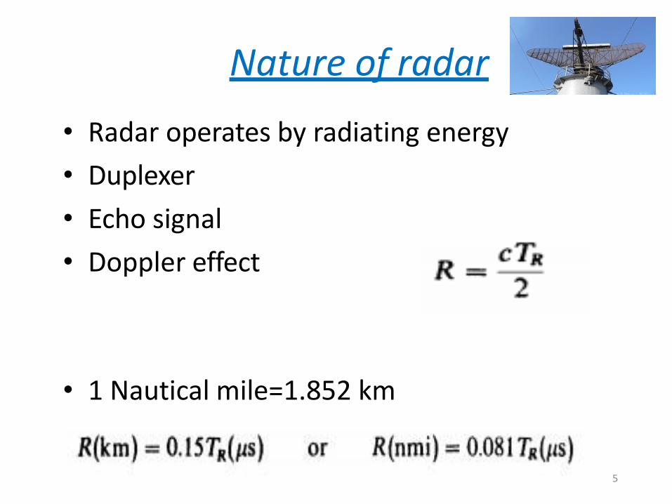
Nature of radar
• Radar operates by radiating energy
• Duplexer
• Echo signal
• Doppler effect
• 1 Nautical mile=1.852 km
5

Maximum Unambiguous Range
• Echoes that arrive after the transmission of the next pulse are called second-time- around(or multiple-time-around) echoes.
• The range beyond which targets appear as second-time-around echoes is called the
Maximu m unambiguous range
6
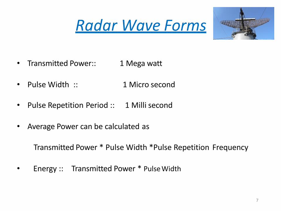
Radar Wave Forms
• Transmitted Power:: 1 Mega watt
• Pulse Width :: 1 Micro second
• Pulse Repetition Period :: 1 Milli second
• Average Power can be calculated as
Transmitted Power * Pulse Width *Pulse Repetition Frequency
• Energy :: Transmitted Power * Pulse Width
7
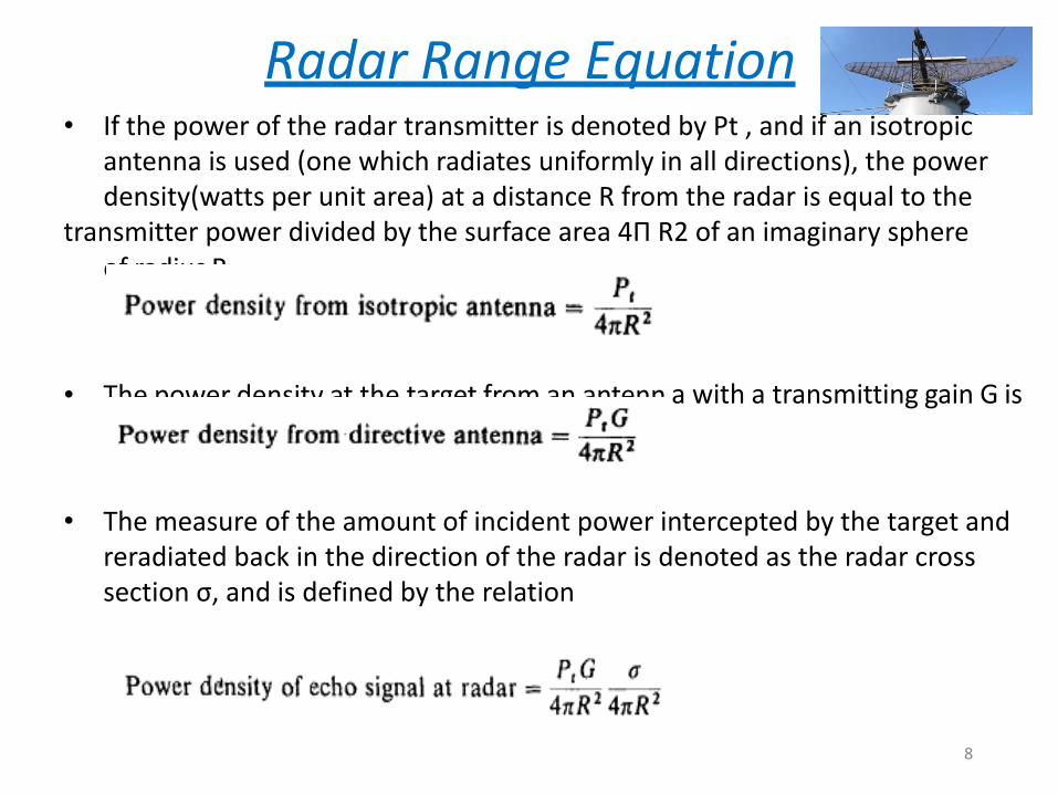
Radar Range Equation • If the power of the radar transmitter is denoted by Pt , and if an isotropic
antenna is used (one which radiates uniformly in all directions), the power density(watts per unit area) at a distance R from the radar is equal to the
transmitter power divided by the surface area 4Π R2 of an imaginary sphere of radius R,
• The power density at the target from an antenn a with a transmitting gain G is
• The measure of the amount of incident power intercepted by the target and reradiated back in the direction of the radar is denoted as the radar cross section σ, and is defined by the relation
8
Radar Range Equation
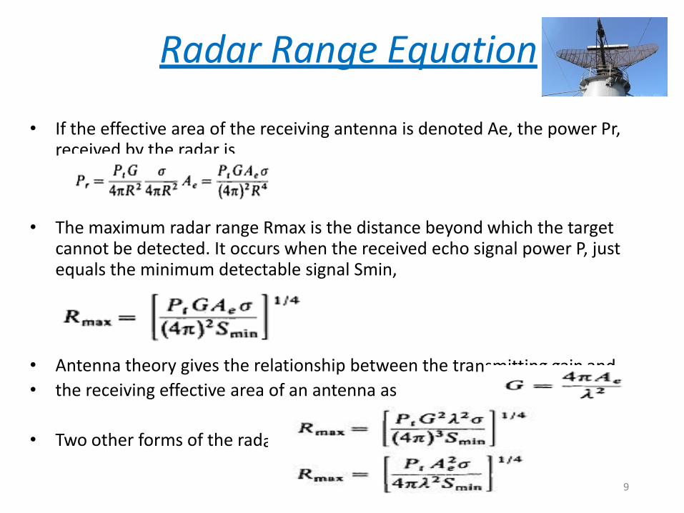
• If the effective area of the receiving antenna is denoted Ae, the power Pr, received by the radar is
• The maximum radar range Rmax is the distance beyond which the target cannot be detected. It occurs when the received echo signal power P, just equals the minimum detectable signal Smin,
nsmitting gain and
ar
• Antenna theory gives the relationship between the tra
• the receiving effective area of an antenna as
• Two other forms of the rad equation
9
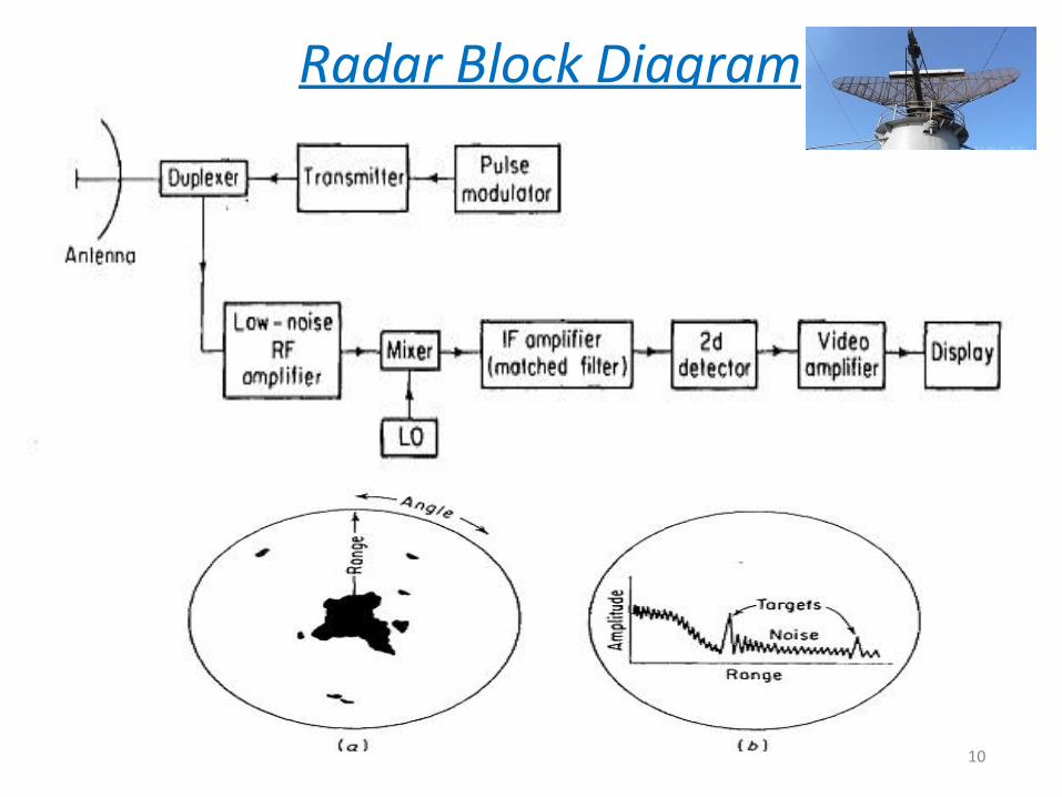
Radar Block Diagram
10

Radar Frequencies
11
Radar Applications
• Air Traffic Control (ATC)
• Aircraft Navigation
• Ship Safety
• Remote Sensing
• Space
• Law Enforcement
• Military
12

RADAR EQUATIONS
Prediction of Range Performance
Minimum Detectable Signal
Receiver Noise and SNR
Integration of Radar pulses
Radar Cross Section of targets
Transmitted Power
Pulse Repetition Frequencies
System Losses
13
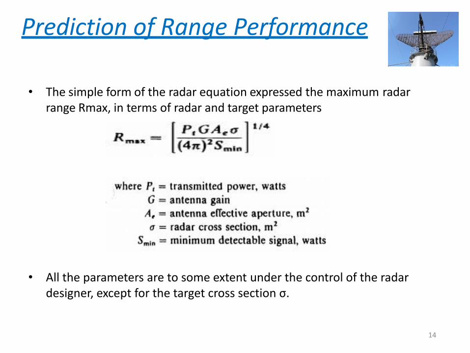
Prediction of Range Performance
• The simple form of the radar equation expressed the maximum radar range Rmax, in terms of radar and target parameters
• All the parameters are to some extent under the control of the radar designer, except for the target cross section σ.
14
Minimum Detectable Signal
• The weakest signal the receiver can detect is called the minimum detectable signal.
• A matched filter for a radar transmitting a rectangular- shaped pulse is usually characterized by a bandwidth B approximately the reciprocal of the pulse width τ,
or Bτ ≈ 1
• Detection is based on establishing a threshold level at the output of the receiver.
• If the receiver output exceeds the threshold, a signal is assumed to be present. This is called threshold detection.
15
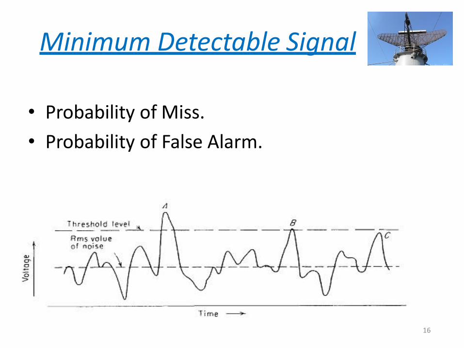
Minimum Detectable Signal
• Probability of Miss.
• Probability of False Alarm.
16
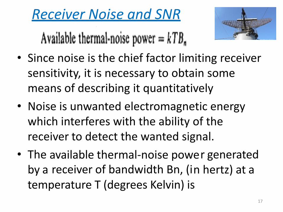
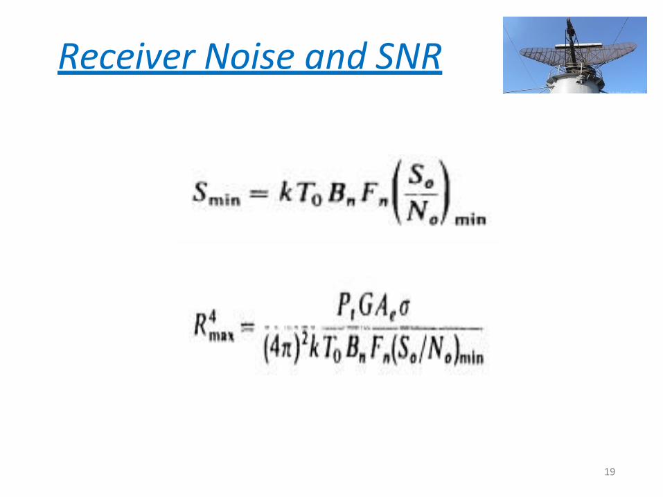
Receiver Noise and SNR
• Since noise is the chief factor limiting receiver sensitivity, it is necessary to obtain some means of describing it quantitatively
• Noise is unwanted electromagnetic energy which interferes with the ability of the receiver to detect the wanted signal.
• The by a
available thermal-noise powe receiver of bandwidth Bn, (i
r generated n hertz) at a
temperature T (degrees Kelvin) is 17

Receiver Noise and SNR
• where k = Boltzmann's constant = 1.38 x 10⁻²³ J/deg.
• Bandwidth and is given by
• If the minimum detectable signal Smin, is that value of Si corresponding to the minimum ratio of output (IF) signal-to-noise ratio (So /No)min necessary for detection.
18
Receiver Noise and SNR
19
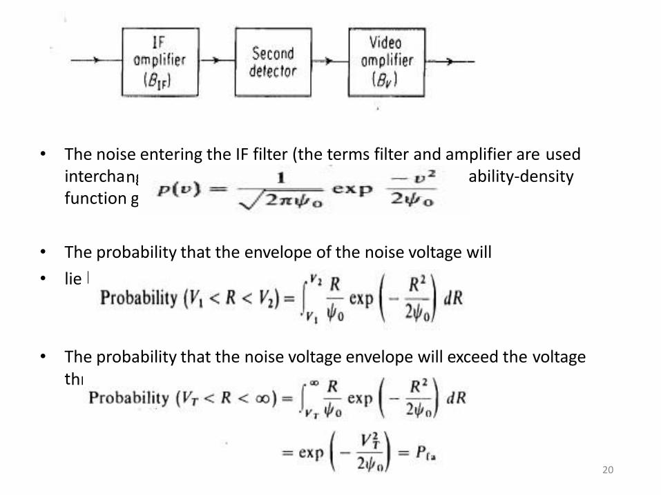
ngeably) is assumed to be guassian, with prob iven by
• The noise entering the IF filter (the terms filter and amplifier are used intercha ability-density function g
• The probability that the envelope of the noise voltage will
• lie between the values of V1 and V2 is
• The probability that the noise voltage envelope will exceed the voltage t hreshold VT is
20
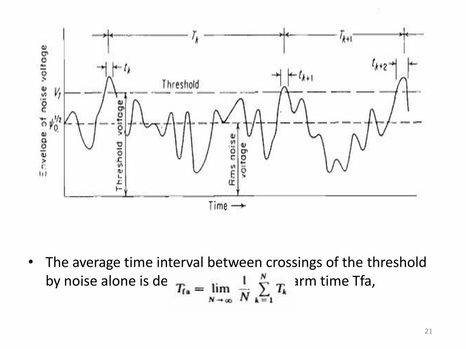
fined as the false-al • The average time interval between crossings of the threshold
by noise alone is de arm time Tfa,
21

• Consider sine-wave signals of amplitude A to be present along with noise at the input to the IFfilter. The frequency of the signal is the same as the IF midband frequency fIF. The output or theenvelope detector has a probability-de nsity function given by
• where Io (Z) is the modified Bessel function of zero order and argument Z
22
es
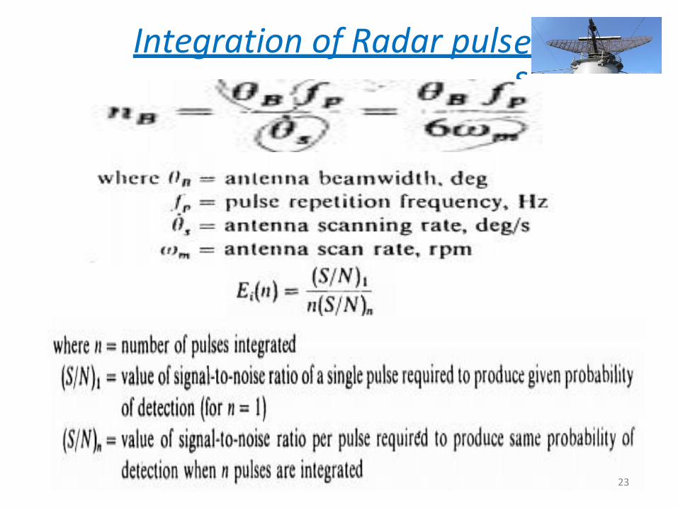
Integration of Radar puls
23
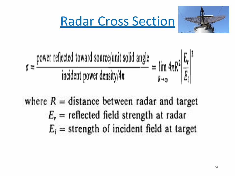
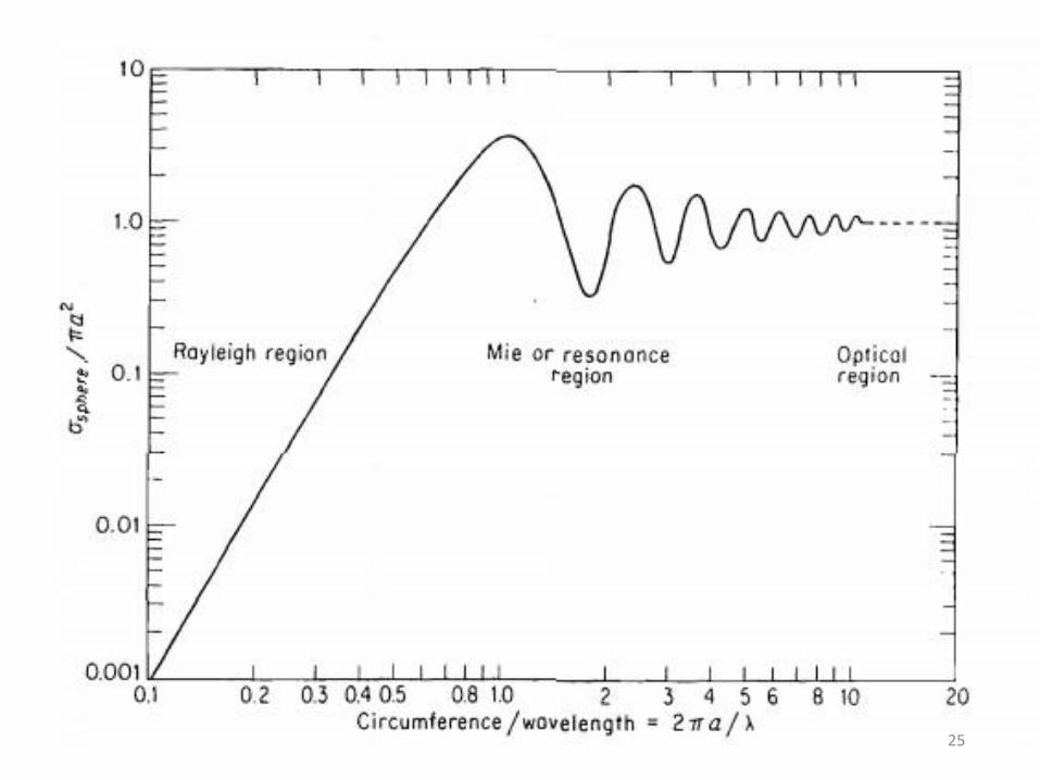
Radar Cross Section
24
25
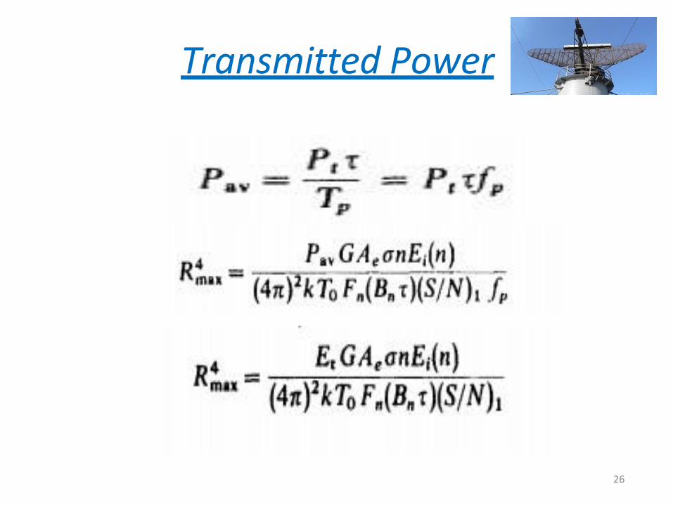
Transmitted Power
26
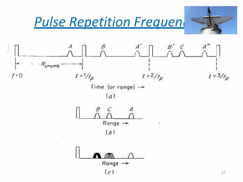
cies Pulse Repetition Frequen
27
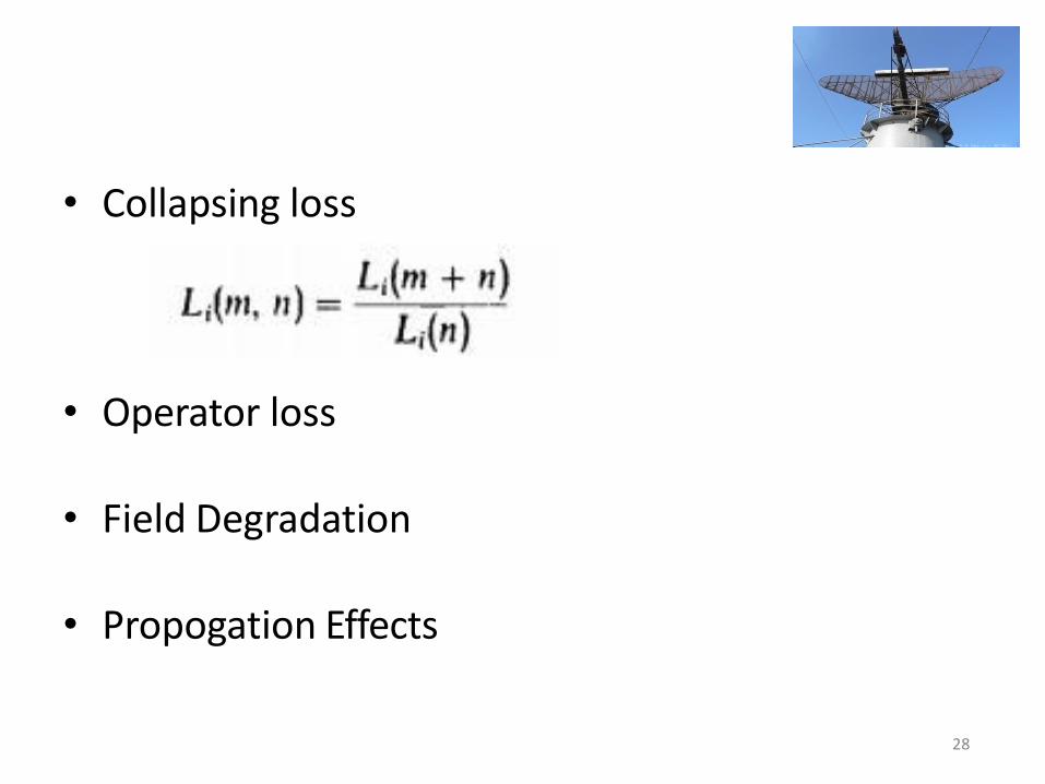
• Collapsing loss
• Operator loss
• Field Degradation
• Propogation Effects
28

CONTENTS :: UNIT-II
Doppler Effect CW Radar Block Diagram Isolation Between Transmitter and Receiver Non Zero IF Receiver Receiver Bandwidth Requirements Identification of Doppler Direction in CW
Radar Applications of CW Radar CW Radar Tracking Illuminator
29
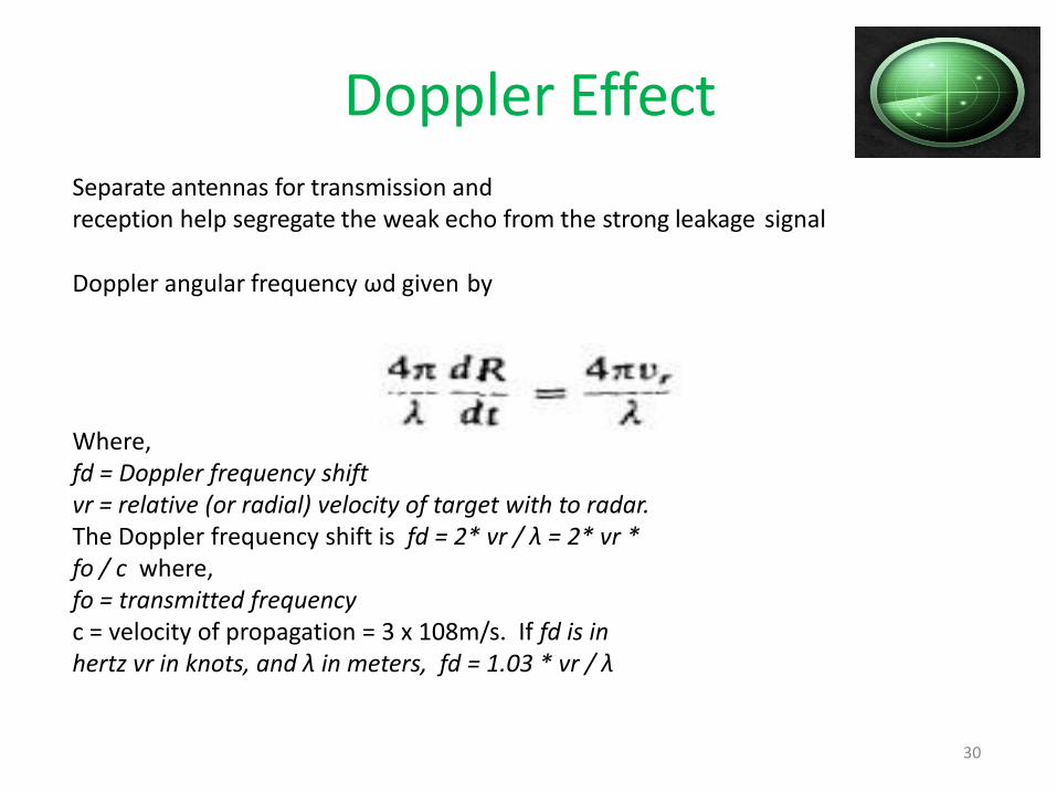
Doppler Effect Separate antennas for transmission and reception help segregate the weak echo from the strong leakage signal
Doppler angular frequency ωd given by
Where, fd = Doppler frequency shift vr = relative (or radial) velocity of target with to radar. The Doppler frequency shift is fd = 2* vr / λ = 2* vr * fo / c where, fo = transmitted frequency c = velocity of propagation = 3 x 10⁸m/s. If fd is in hertz vr in knots, and λ in meters, fd = 1.03 * vr / λ
30
Doppler Effect
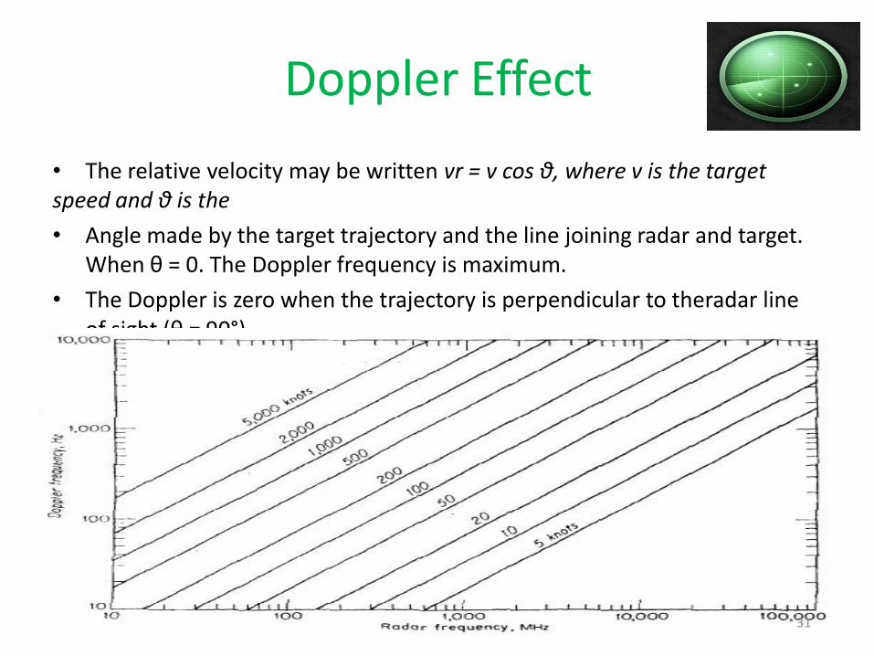
• The relative velocity may be written vr = v cos θ, where v is the target speed and θ is the
• Angle made by the target trajectory and the line joining radar and target. When θ = 0. The Doppler frequency is maximum.
• The Doppler is zero when the trajectory is perpendicular to theradar line of sight (θ = 90°).
31
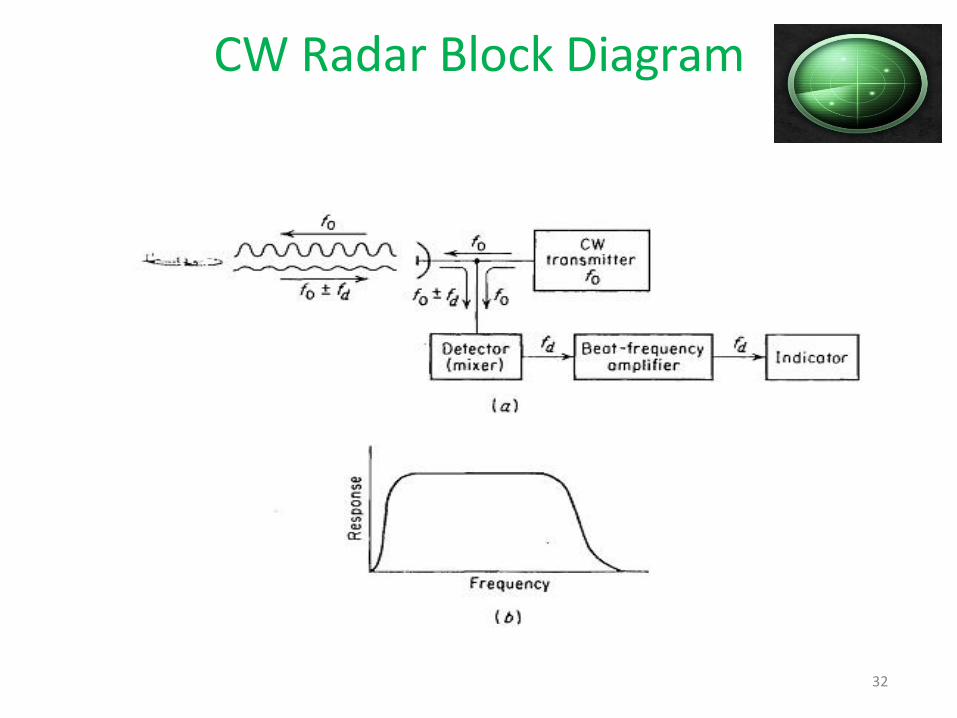
CW Radar Block Diagram
32
Isolation Between Transmitter a nd Receiver
• Isolation betweenthe transmitted and the received signals is achieved via separation in frequency as a result of the doppler effect.
• There are two practical effects which limit the amount of transmitter leakage power which can be tolerated at the receiver.
• (1) The maximum amount of power the receiver input circuitry can withstand before it is physically damaged or its sensitivity reduced
• (2) The amount of transmitter noise due to hum, microphonics etc.
33
and Isolation Between Transmitter Receiver
• The amount of isolation which can be readily achieved
between the arms of practical hybrid junctions such as
the magic-T is of the order of 20 to 30 dB.
• Separate polarizations
• VSWR
• Separate antennas
• Dynamic cancellation of leakage
34
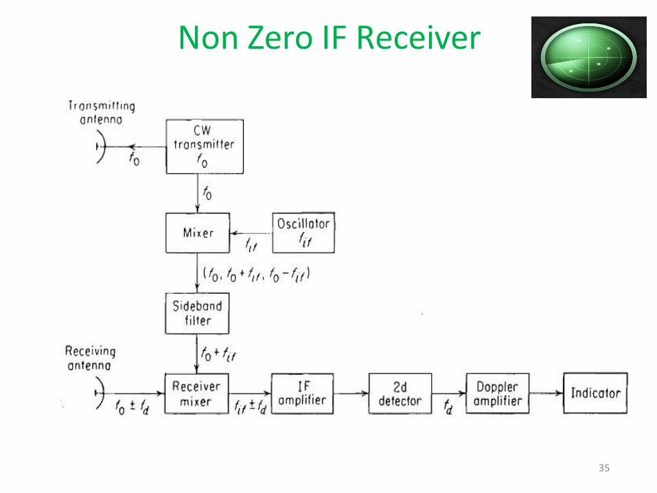
Non Zero IF Receiver
35
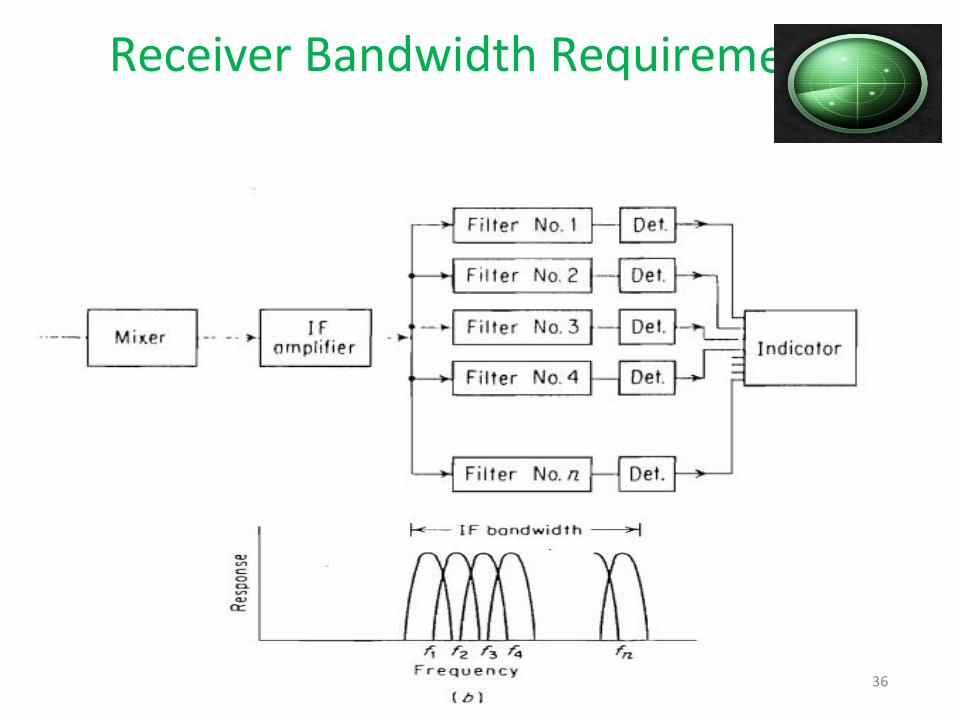
Receiver Bandwidth Requirem ents
36
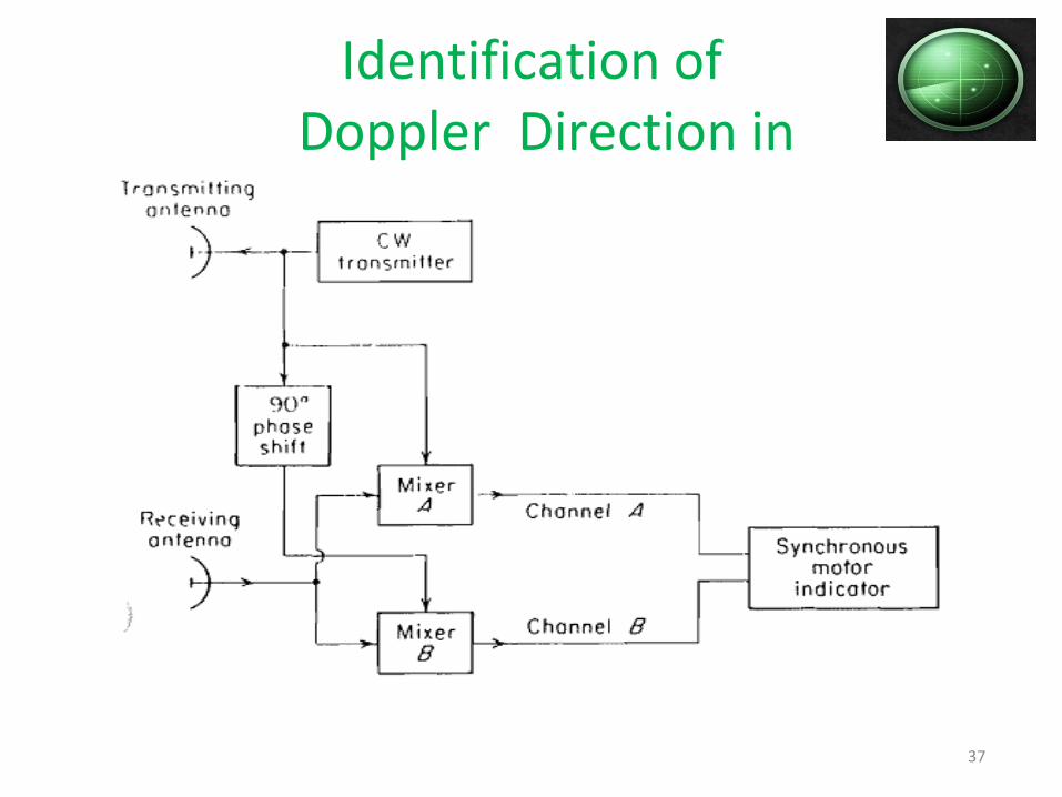
Identification of Doppler Direction in
CW Radar
37

Identification of Doppler Direction in
CW Radar • If the target is approaching (positive Doppler), the outputs from the two channels are
EA ( + ) = K2 E0 cos (wd t + φ ) EB ( + )= K2 E0 cos (wd t + φ + π / 2 )
• If the targets are receding (negative doppler), the outputs from the two channels are EA ( - ) = K2 E0 cos (wd t - φ ) EB ( - )= K2 E0 cos (wd t - φ - π / 2 ) • The direction of motor rotation is an indication of
the direction of the target motion.
38

Applications of CW Radar
• Police speed monitor
• Collision avoidance.
• Control of traffic lights
• CW radar can be used as a speedometer to replace the
conventional tachometer in Railways
• Warning of approaching trains.
• Speed of large ships.
• Velocity of missiles
39

CW Radar Tracking Illuminato r
40

FM-CW RADAR
FMCW Radar
Range and Doppler Measurement
Approaching and Receding Targets
FMCW Altimeter
Measurement Errors
Unwanted Signals
Sinusoidal Modulation
Multiple Frequency CW Radar
41

FMCW Radar
42
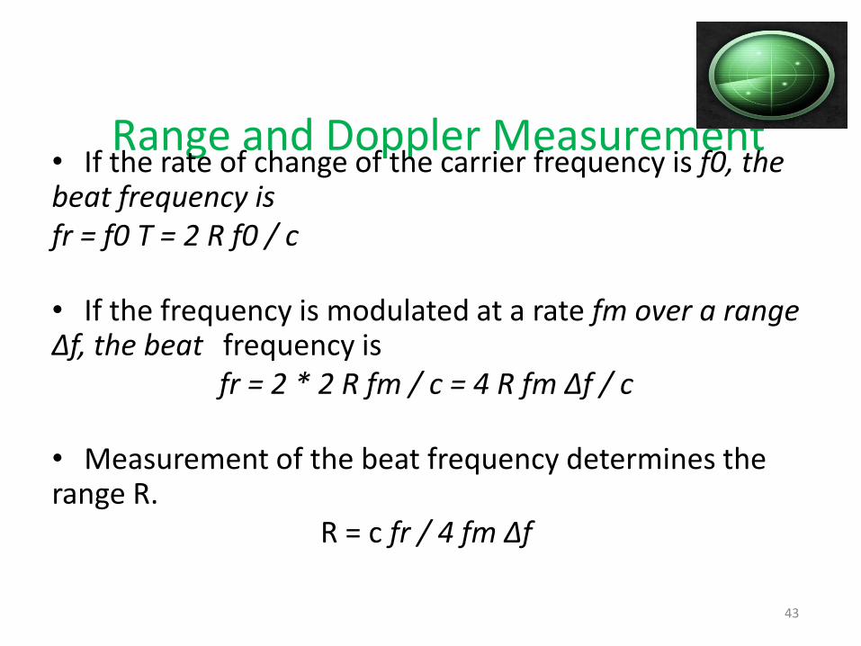
Range and Doppler Measurement • If the rate of change of the carrier frequency is f0, the beat frequency is fr = f0 T = 2 R f0 / c
• If the frequency is modulated at a rate fm over a range Δf, the beat frequency is
fr = 2 * 2 R fm / c = 4 R fm Δf / c
• Measurement of the beat frequency determines the range R.
R = c fr / 4 fm Δf
43
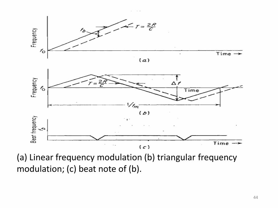
Range and Doppler Measurement
(a) Linear frequency modulation (b) triangular frequency modulation; (c) beat note of (b).
44
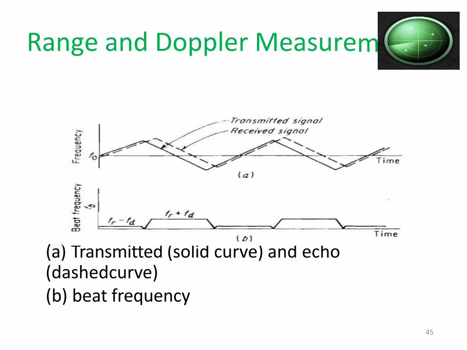
Range and Doppler Measure ment
(a) Transmitted (solid curve) and echo (dashedcurve) (b) beat frequency
45
Approaching and Receding Targets
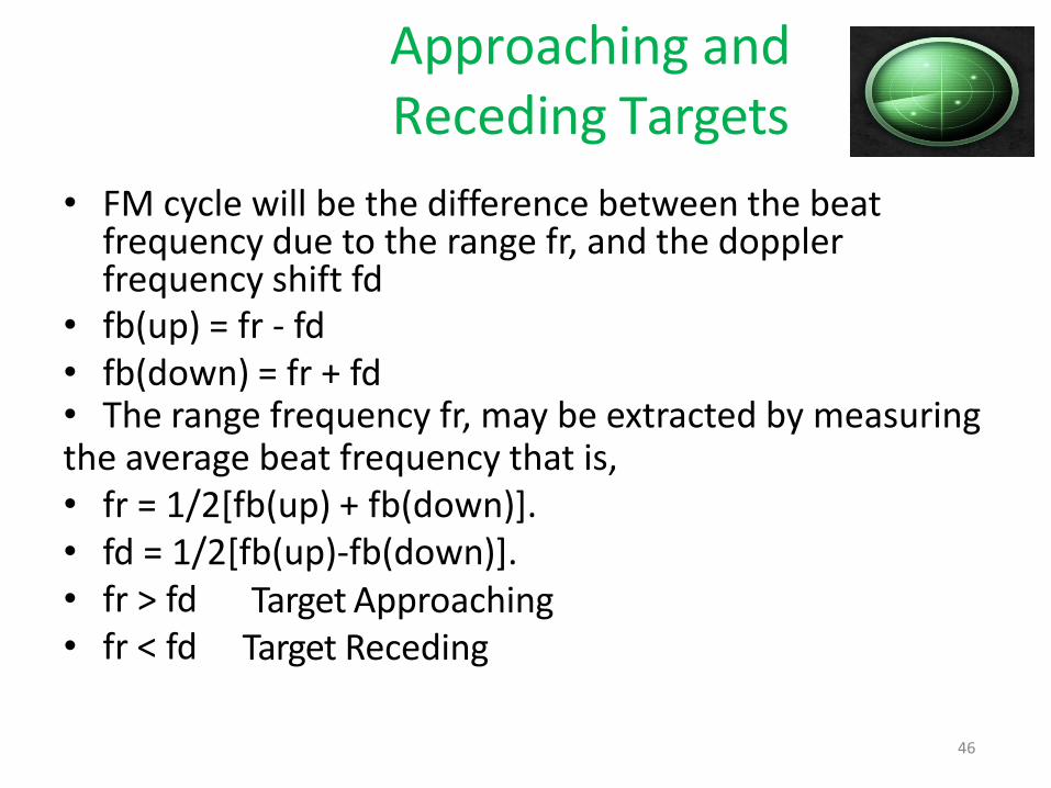
• FM cycle will be the difference between the beat frequency due to the range fr, and the doppler frequency shift fd
• fb(up) = fr - fd • fb(down) = fr + fd • The range frequency fr, may be extracted by measuring the average beat frequency that is, • fr = 1/2[fb(up) + fb(down)]. • fd = 1/2[fb(up)-fb(down)]. • fr > fd • fr < fd
Target Approaching Target Receding
46
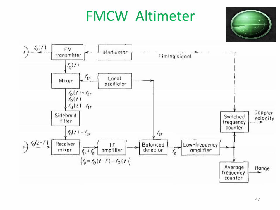
FMCW Altimeter
47

Measurement Errors
• The average number of cycles N of the beat frequency fb in one period of the modulation cycle fm is fb /fm , where the bar over , denotes time average.
• Which measures the number of cycles or half cycles of the beat during the modulation period.
• The total cycle count is a discrete- number since the counter is unable to measure fractions of a cycle.
• The discreteness of the frequency measurement gives rise to an error called the fixed error, or step erroror quantization error
48

Measurement Errors
• R = c N / 4 Δ f • Where, R = range (altitude). m c = velocity of propagation. m/s Δf = frequency
excursion. Hz • Since the output of the frequency counter N is an
integer, the range will be an integral multiple of c / 4 Δ f and will give rise to a quantization error equal to
δ R = c / 4 Δ f δ R (m) = 75 / Δ f ( MHz)
49
Unwanted Signals
50

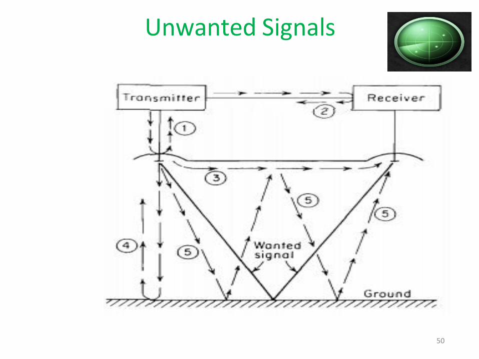
Unwanted Signals
•The Unwanted signals include 1.Transmitting Antenna
impedance mismatch 2.Receiver poor mixer match.
3.Coupling between transmitter and receiver antennas
4.The interference due to power being reflected back to
the transmitter
5. The double-bounce signal.
51

Sinusoidal Modulation
fm.
be
• If the CW carrier is frequency-modulated by a sine wave, the difference frequency obtained by heterodyning the returned signal with a portion of the transmitter signal may be expanded in a trigonometric series whose terms are the harmonics of the modulating frequency
• Assume the formwohfereth, e transmitted signal to fo = carrier frequency
fm = modulation frequency Δf = frequency excursion
52
Sinusoidal Modulation
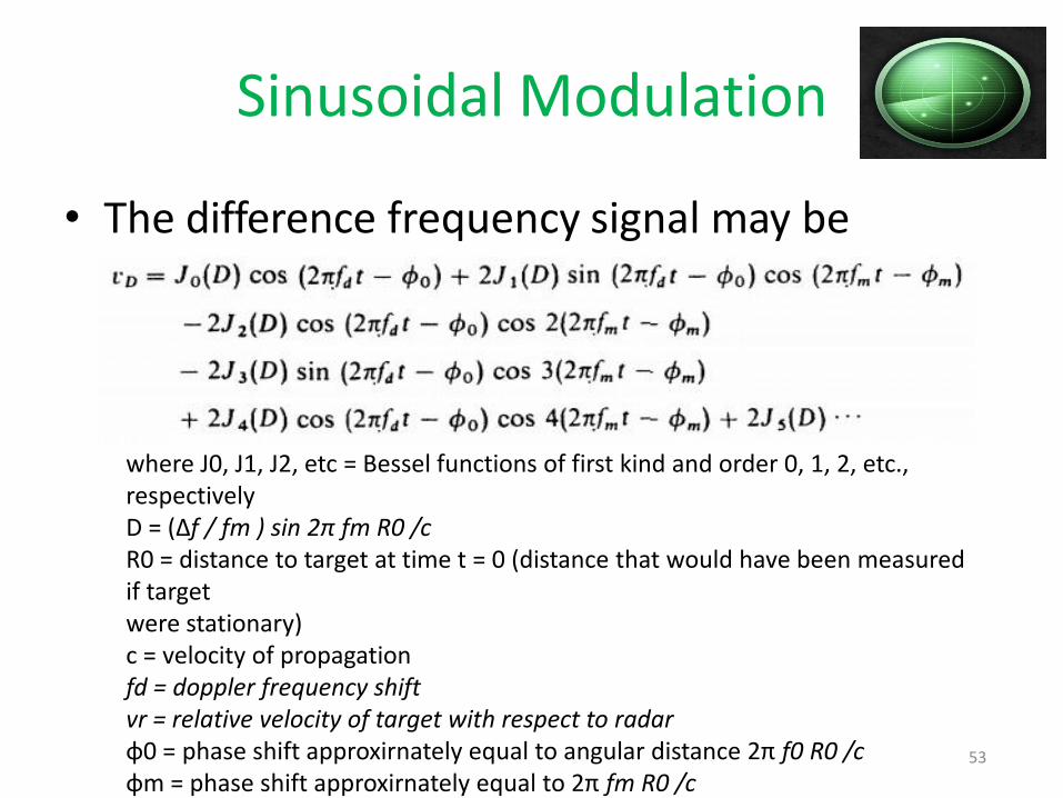
• The difference frequency signal may be written as
where J0, J1, J2, etc = Bessel functions of first kind and order 0, 1, 2, etc., respectively D = (Δf / fm ) sin 2π fm R0 /c R0 = distance to target at time t = 0 (distance that would have been measured if target were stationary) c = velocity of propagation fd = doppler frequency shift vr = relative velocity of target with respect to radar φ0 = phase shift approxirnately equal to angular distance 2π f0 R0 /c φm = phase shift approxirnately equal to 2π fm R0 /c
53

Sinusoidal Modulation (3rd Harmonic) Extraction
54
Multiple Frequency CW Rad ar
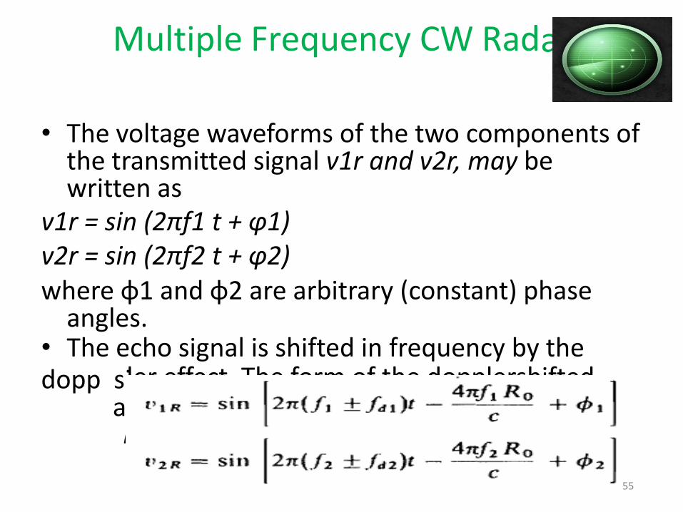
• The voltage waveforms of the two components of the transmitted signal v1r and v2r, may be written as
v1r = sin (2πf1 t + φ1) v2r = sin (2πf2 t + φ2) where φ1 and φ2 are arbitrary (constant) phase
angles. • The echo signal is shifted in frequency by the dopp sign may ler effect. The form of the dopplershifted
als at each of the two frequencies f1 and f2 be written as
55
Multiple Frequency CW Ra dar
• Where, Ro = range to target at a particular time t = t0 (range that would be measured if target were not moving)
• fd1 = doppler frequency shift associated with frequency f1
• fd2 = doppler frequency shift associated with frequency f2 • Since the two RF frequencies f1 , and f2 are
approximately the same the doppler frequency shifts fd1 and fd2 are approximately equal to one another. Therefore
• fd1 = fd2 = fd
56
Multiple Frequency CW Ra dar
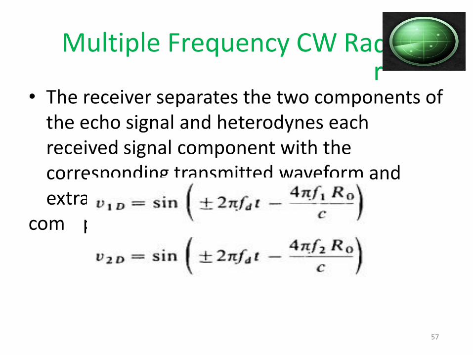
• The receiver separates the two components of the echo signal and heterodynes each received signal component with the corresponding transmitted waveform and extra
com cts the two doppler-frequency
ponents given below:
57
Multiple Frequency CW Ra dar
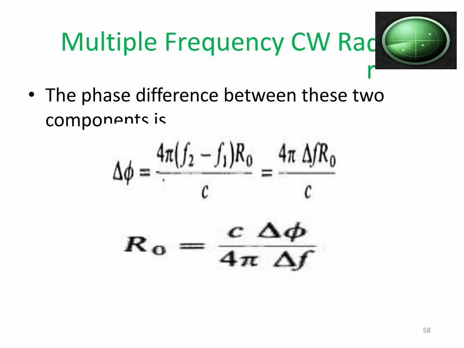
• The phase difference between these two components is
58
Multiple Frequency CW Ra dar
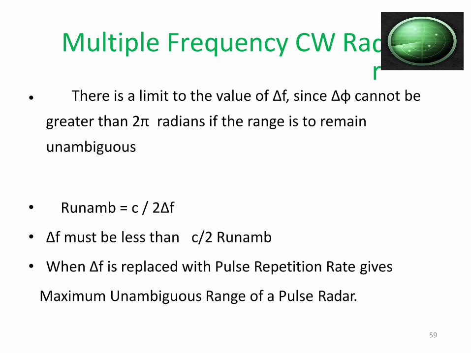
• There is a limit to the value of Δf, since Δφ cannot be
greater than 2π radians if the range is to remain
unambiguous
• Runamb = c / 2Δf
• Δf must be less than c/2 Runamb
• When Δf is replaced with Pulse Repetition Rate gives
Maximum Unambiguous Range of a Pulse Radar.
59

n
n
Moving Target Indicator Radar (MTI) Clutter is the term used for radar targets which are not of interest to the user.
Clutter is usually caused by static objects near the radar but sometimes far away as well:
UNIT III
60
Moving Target Indicator Radar (MTI)
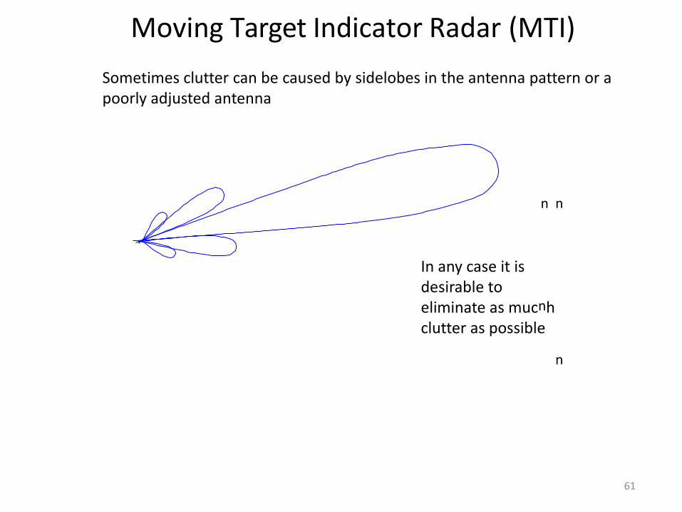
Sometimes clutter can be caused by sidelobes in the antenna pattern or a poorly adjusted antenna
n n
In any case it is desirable to eliminate as mucnh clutter as possible
n
61
Moving Target Indicator Radar (MTI)
n
n
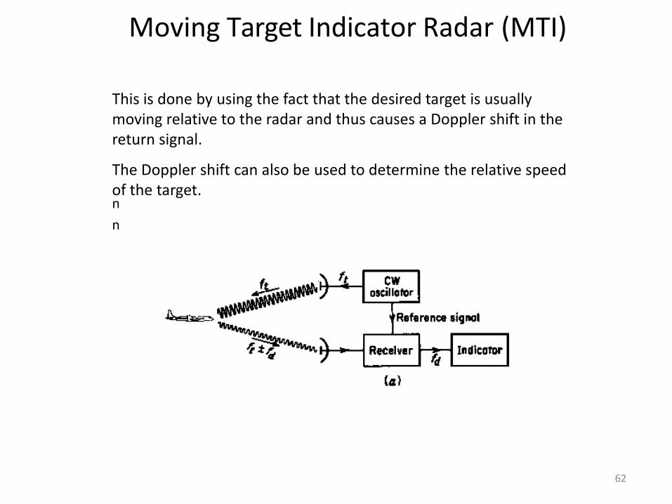
This is done by using the fact that the desired target is usually moving relative to the radar and thus causes a Doppler shift in the return signal.
The Doppler shift can also be used to determine the relative speed of the target. n
n
62
Moving Target Indicator Radar (MTI)
n
n
n
n
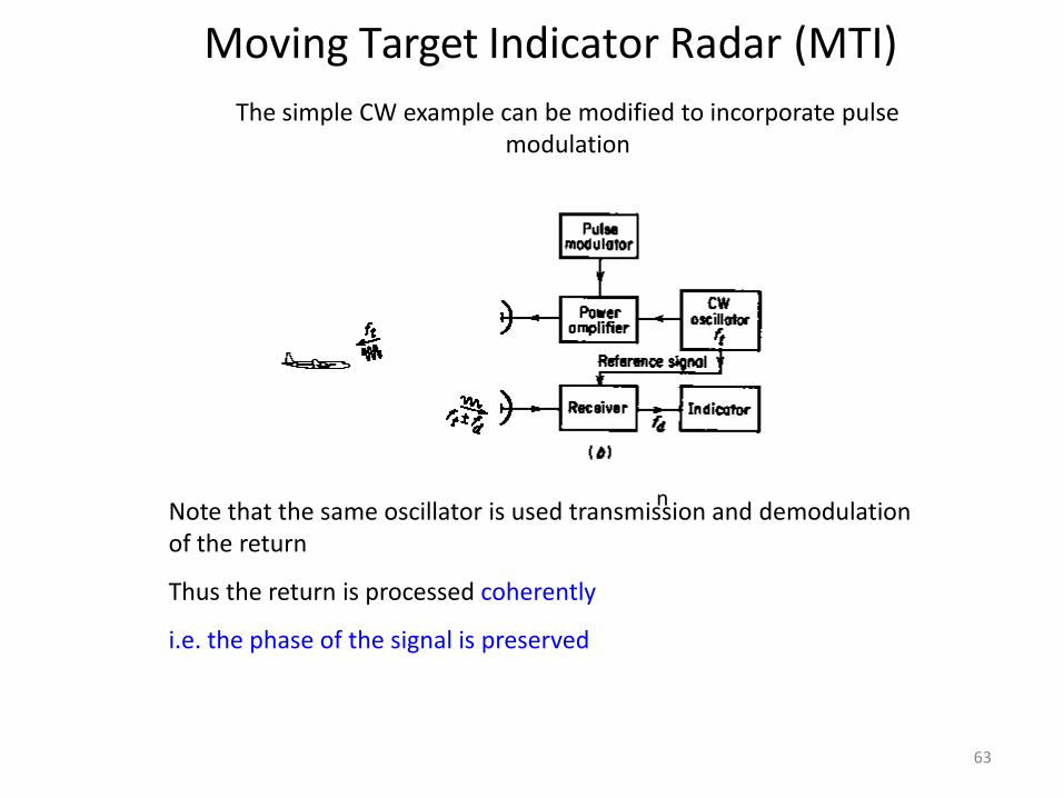
The simple CW example can be modified to incorporate pulse modulation
Note that the same oscillator is used transmission and demodulation of the return
Thus the return is processed coherently
i.e. the phase of the signal is preserved
63

Moving Target Indicator Radar (MTI)
n
n
The transmitted signal is
and the received signal is
these are mixed and the difference is extracted
64
n
This has two components, one is a sine wave at Doppler frequency, the other is a phase shift which depends on the range to the tarnget, R0

Moving Target Indicator Radar (MTI)
n
n
n
Note that for stationary targets fd = 0 so Vdiff is constant
Depending on the Doppler frequency one two situations will occur n
fd>1/τ
65
fd<1/τ
66
Moving Target Indicator Radar (MTI)
n
n
n
n
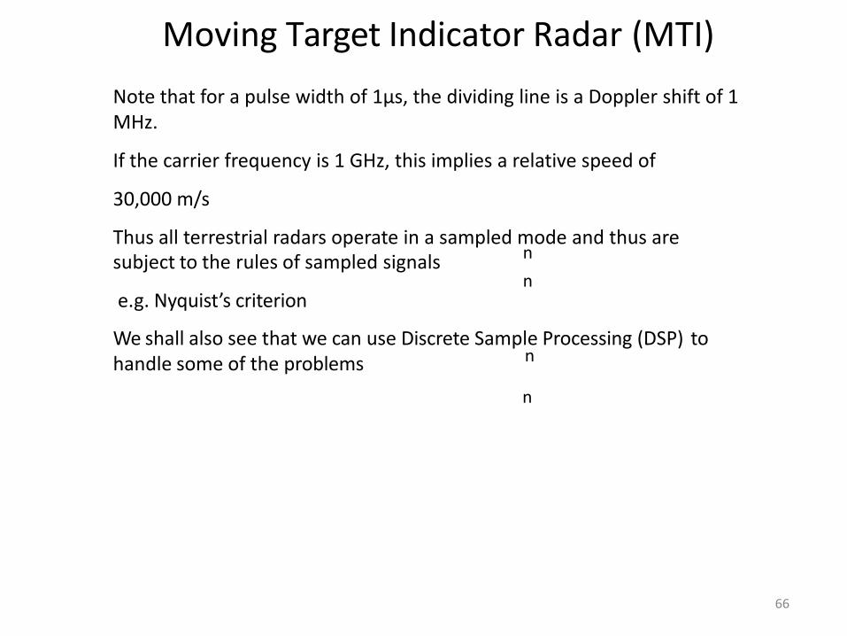
Note that for a pulse width of 1μs, the dividing line is a Doppler shift of 1 MHz.
If the carrier frequency is 1 GHz, this implies a relative speed of
30,000 m/s
Thus all terrestrial radars operate in a sampled mode and thus are subject to the rules of sampled signals
e.g. Nyquist’s criterion
We shall also see that we can use Discrete Sample Processing (DSP) to handle some of the problems
Moving Target Indicator Radar (MTI)
n
n
n
n
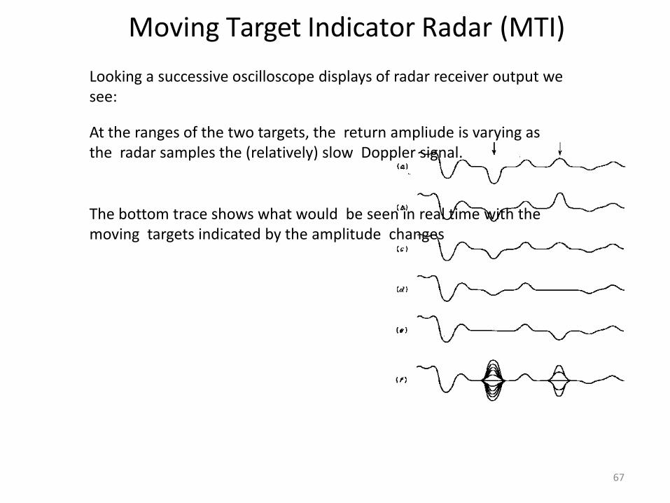
Looking a successive oscilloscope displays of radar receiver output we see:
At the ranges of the two targets, the return ampliude is varying as the radar samples the (relatively) slow Doppler signal.
The bottom trace shows what would be seen in real time with the moving targets indicated by the amplitude changes
67

Moving Target Indicator Radar (MTI)
n
n
n
We usually want to process the information automatically. To do this we take advantage of the fact that the amplitudes of successive pulse returns are different:
z-1
68
OR n
-
Moving Target Indicator Radar (MTI)
n
n
n
n
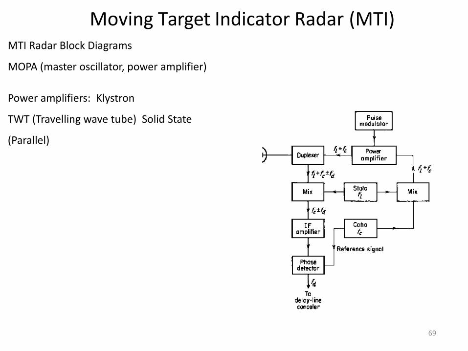
MTI Radar Block Diagrams
MOPA (master oscillator, power amplifier)
Power amplifiers: Klystron
TWT (Travelling wave tube) Solid State
(Parallel)
69

70
Moving Target Indicator Radar (MTI)
n
n
n
n
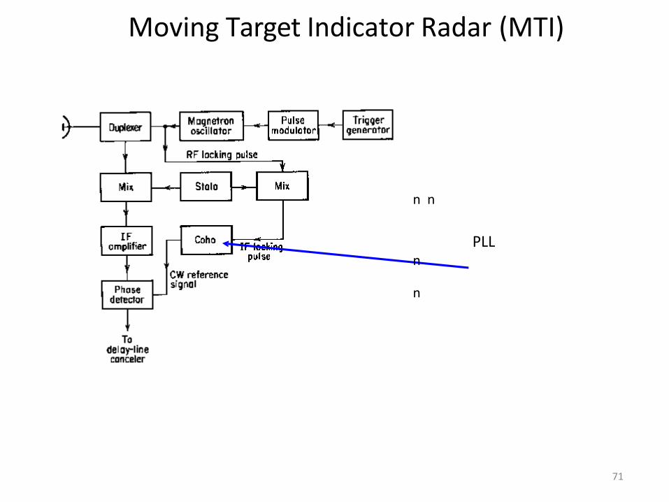
One of the problems with MTI in pulsed radars is that magnetrons are ON/OFF devices.
i.e. When the magnetron is pulsed it starts up with a random phase and is thus its ouput is not coherent with the pulse before it. Also it can not provide a reference oscillator to mix with the received signals.
Therefore some means must be provided to maintain the coherence (at least during a single pulse period)
Moving Target Indicator Radar (MTI)
n n
PLL
n
n
71
72
Moving Target Indicator Radar (MTI)
The notes have a section on various types of delay line cancellers.
This is a bit out of date because almost all radars today
use digitized data and implementing the required delays is relatively trivial but it also opens up much more complex processing possibilities
n n
n
n

Moving Target Indicator Radar (MTI)
n
n
n
n
The Filtering Characteristics of a Delay Line Canceller
The output of a single delay canceller is:
This will be zero whenever πfdT is 0 or a multiple of π
The speeds at which this occurs are called the blind
speeds of the radar
. where n is 0,1,2,3,…
73

74
Moving Target Indicator Radar (MTI)
If the first blind speed is to be greater than the highest expected radial speed the λfp must be large
large λ means larger antennas for a given beamwidth
large fp means that the unambiguous range will be quitensmall
n
So there has to be a compromise in the design of an MTI radar
n
n

75
Moving Target Indicator Radar (MTI)
n
n
n
n
The choice of operating with blind speeds or ambiguous ranges depends on the application
Two ways to mitigate the problem at the expense of increased complexity are:
a. operating with multiple prfs b. operating with multiple carrier frequencies

76
Moving Target Indicator Radar (MTI)
n
n
n
n
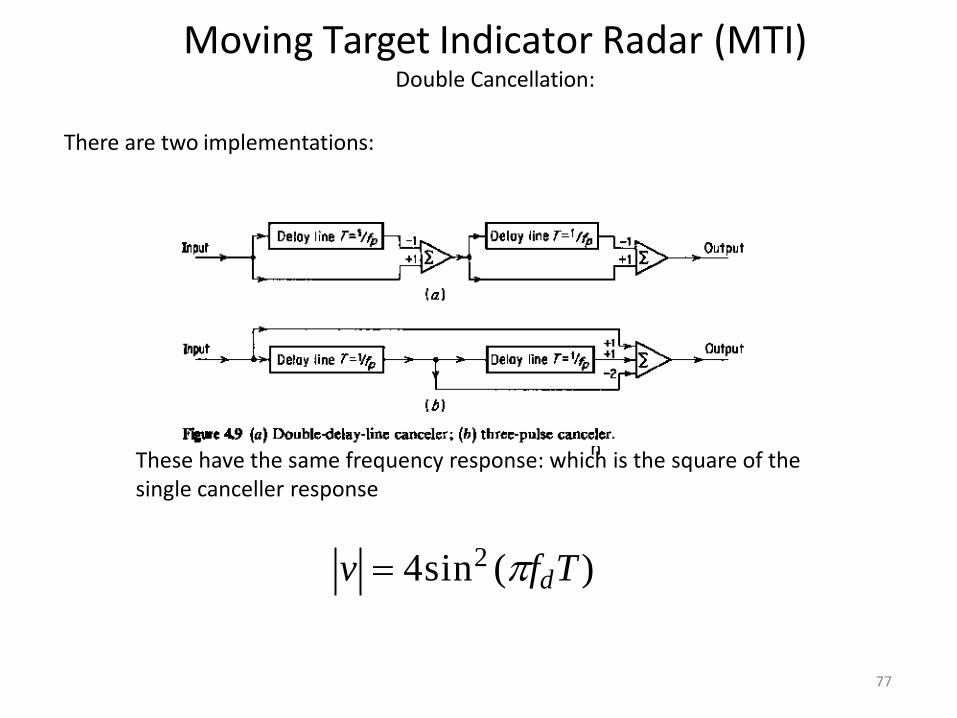
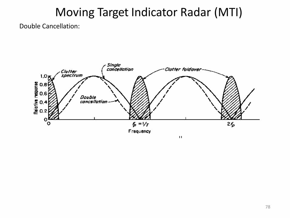
Double Cancellation:
Single cancellers do not have a very sharp cutoff at the nulls which limits their rejection of clutter
(clutter does not have a zero width spectrum)
Adding more cancellers sharpens the nulls
n
n
n
n
Moving Target Indicator Radar (MTI) Double Cancellation:
There are two implementations:
These have the same frequency response: which is the square of the single canceller response
v 4sin2 (fd T )
77
n
n
n
n
Moving Target Indicator Radar (MTI) Double Cancellation:
78
Moving Target Indicator Radar (MTI)
n
n
n
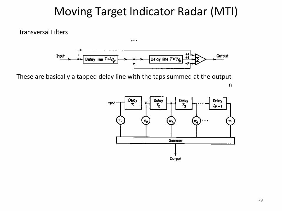
Transversal Filters
These are basically a tapped delay line with the taps summed at the output n
79
Moving Target Indicator Radar (MTI)
n
n
n
n
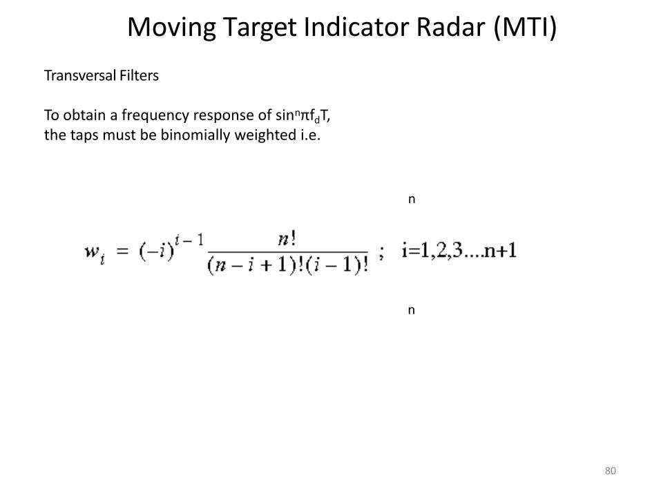
Transversal Filters
To obtain a frequency response of sinnπfdT, the taps must be binomially weighted i.e.
80

Moving Target Indicator Radar (MTI)
n
n
n
Filter Performance Measures MTI Improvement Factor, IC
in C I
(S / C)
(S / C)out
Note that this is averaged over all Doppler frequencies
n
1/2T 0
Signal Clutter
1/2T 0
Filter
81
82
Moving Target Indicator Radar (MTI)
Filter Performance Measures
Clutter Attenuation ,C/A
The ratio of the clutter power at the input of the canceler
to the clutter power at the output of the cancelern
n It is normalized, (or adjusted) to the signal attenuation of the canceler.
i.e. the inherent signal attenuation of the cancelernis ignored
n
Moving Target Indicator Radar (MTI)
n
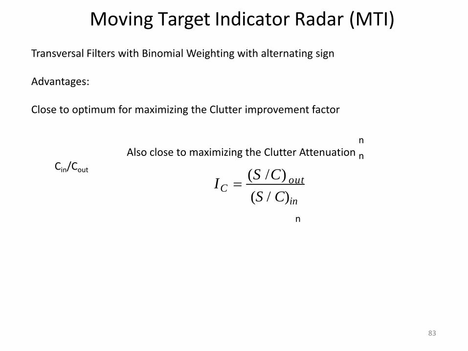
Transversal Filters with Binomial Weighting with alternating sign
Advantages:
Close to optimum for maximizing the Clutter improvement factor
n
Also close to maximizing the Clutter Attenuation n Cin/Cout
(S / C)in
n
83
(S / C) IC out
Moving Target Indicator Radar (MTI)
n
n
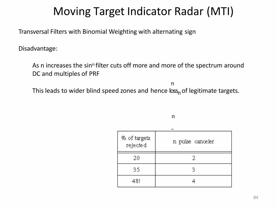
Transversal Filters with Binomial Weighting with alternating sign
Disadvantage:
As n increases the sinn filter cuts off more and more of the spectrum around DC and multiples of PRF
n This leads to wider blind speed zones and hence lossn of legitimate targets.
84

85
Moving Target Indicator Radar (MTI)
n
The ideal MTI filter should reject clutter at DC and th PRFs but give a flat pass band at all other frequencies.
The ability to shape the frequency response depends to a large degree on the number of pulses used. The more pulses, the more flexibility in the filter design.
Unfortunately the number of pulses is limited by the scnan rate and the antenna beam width.
Note that not all pulses are useful:
n The first n-1 pulses in an n pulse canceler are not useful
n
Moving Target Indicator Radar (MTI)
n
n
n
n
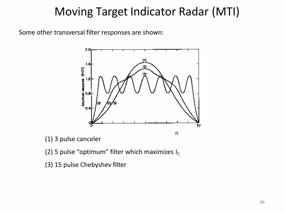
Some other transversal filter responses are shown:
(1) 3 pulse canceler
(2) 5 pulse “optimum” filter which maximizes IC
(3) 15 pulse Chebyshev filter
86

Moving Target Indicator Radar (MTI)
87
Feed forward (finite impulse response or FIR) filters have only poles (one per delay)
More flexibility in filter design can be obtained if we use recursive or feedback filters (also known as infinite impulse response or IIR filters)
These have a zero as well as a pole per delay and thus have twice as many variables to play with
88
Moving Target Indicator Radar (MTI)
IIR filters can be designed using standard continuous-time filter techniques and then transformed into the discrete form using z transforms
Thus almost any kind of frequency response can be obtained with these filters.
They work very well in the steady state case but unfortunately their transient response is not very good. A large pulse input can cause the filter to “ring” and thus miss desired targets.
Since most radars use short pulses, the filters are almost always in a transient state
89
Moving Target Indicator Radar (MTI)
Multiple PRFs
An alternative is to use multiple PRFs because the blind speeds (and hence the shape of the filter response) depends on the PRF and, combining two or more PRFs offers an opportunity to shape the overall response.

Moving Target Indicator Radar (MTI)
Multiple PRFs: Example
Two PRFs
Ratio 4/5
First blind speed is at
5/T1 or 4/T2
90
Moving Target Indicator Radar (MTI)
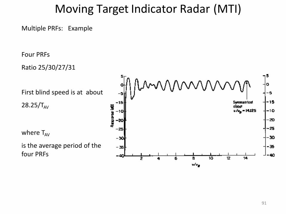
Multiple PRFs: Example
Four PRFs
Ratio 25/30/27/31
First blind speed is at about
28.25/TAV
where TAV
is the average period of the four PRFs
91
Moving Target Indicator Radar (MTI)
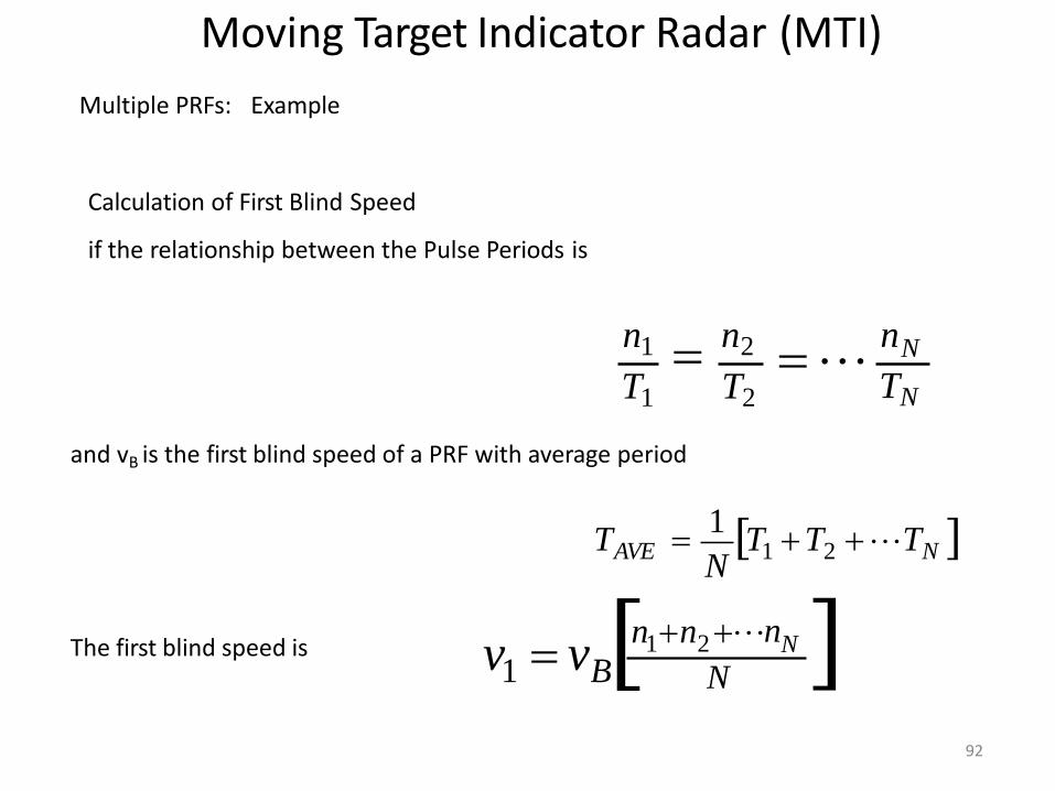
Multiple PRFs: Example
Calculation of First Blind Speed
if the relationship between the Pulse Periods is
N
TN
n
n1 n2
T1 T2
and vB is the first blind speed of a PRF with average period
AVE N
1 2 N T 1 T T T
The first blind speed is 92
N n n n v v 1 2
N 1 B
n
n
n
n
Moving Target Indicator Radar (MTI)
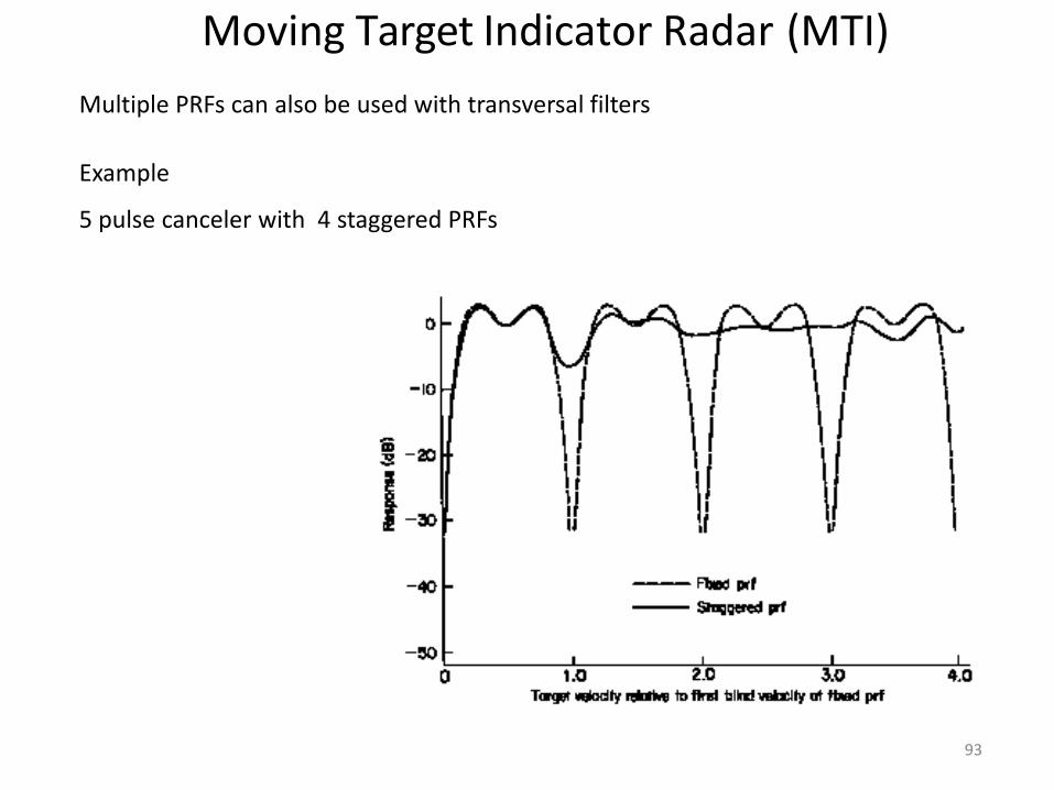
Multiple PRFs can also be used with transversal filters
Example
5 pulse canceler with 4 staggered PRFs
93
Moving Target Indicator Radar (MTI)
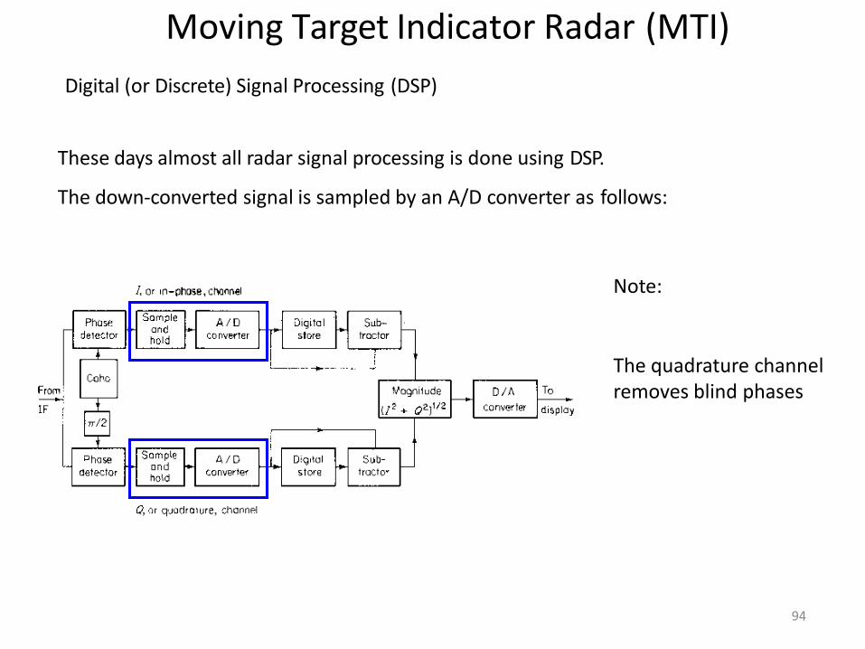
Digital (or Discrete) Signal Processing (DSP)
These days almost all radar signal processing is done using DSP.
The down-converted signal is sampled by an A/D converter as follows:
Note:
The quadrature channel removes blind phases
94
95
Moving Target Indicator Radar (MTI)
•Advantages of DSP
•greater stability
•greater repeatability
•greater precision
•greater reliability
•easy to implement multiple PRFs
•greater flexibility in designing filters
•gives the ability to change the system parameters dynamically
96
Moving Target Indicator Radar (MTI)
Digital (or Discrete) Signal Processing (DSP)
Note that the requirements for the A/D are not very difficult to meet with today’s technology.
Sampling Rate
Assuming a resolution (Rres) of 150m, the received signal has to be sampled at intervals of c/2Rres = 1μs or a sampling rate of 1 MHz
Memory Requirement
Assuming an antenna rotation period of 12 s (5rpm) the storage required would be only 12 Mbytes/scan.
Moving Target Indicator Radar (MTI) Digital (or Discrete) Signal Processing (DSP)
Quantization Noise
The A/D introduces noise because it quantizes the signal
The Improvement Factor can be limited by the quantization noise
the limit being:
IQN 20log(2N 1) 0.75 This is approximately 6 dB per bit
A 10 bit A/D thus gives a limit of 60 dB
In practice one or more extra bits to achieve the desired performance
97
98
Moving Target Indicator Radar (MTI) Digital (or Discrete) Signal Processing (DSP)
Dynamic Range
This is the maximum signal to noise ratio that can be handled by the A/D without saturation
dynamic _ range 22N 3 / k 2
N= number of bits
k=rms noise level divided by the quantization interval the larger k the lower the
dynamic range
but k<1 results in reduction of sensitivity
Note: A 10 bit A/D gives a dynamic range of 45.2dB

Moving Target Indicator Radar (MTI) Blind Phases
If the prf is double the Doppler frequency then every othyer pair of samples cane be the same amplitude and will thus be filtered out of the signal.
By using both inphase and quadrature signals, blind phases can be eliminated
99
Moving Target Indicator Radar (MTI)
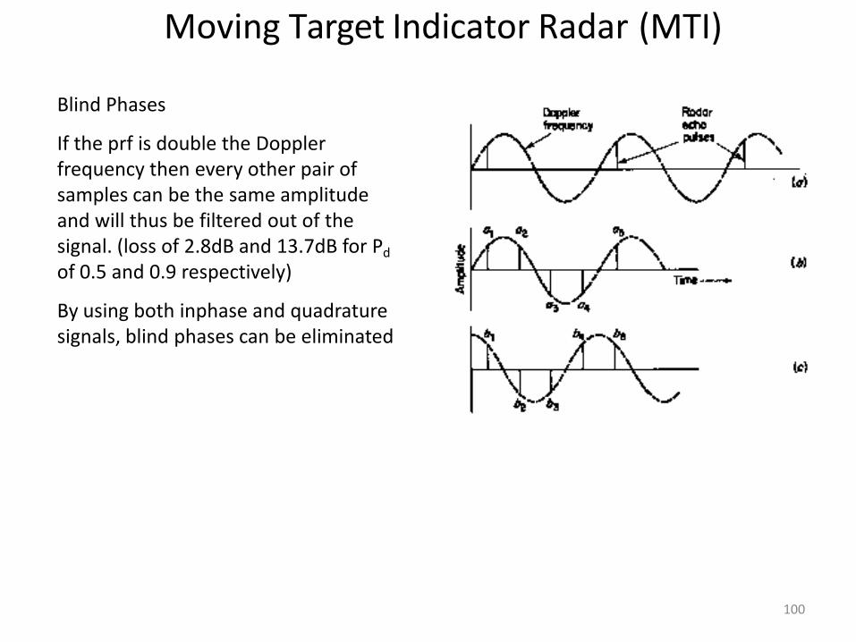
Blind Phases
If the prf is double the Doppler frequency then every other pair of samples can be the same amplitude and will thus be filtered out of the signal. (loss of 2.8dB and 13.7dB for Pd
of 0.5 and 0.9 respectively)
By using both inphase and quadrature signals, blind phases can be eliminated
100
w w w w w w w w
z-1 z-1 z-1 z-1 z-1 z-1 z-1 z-1
SUMMER
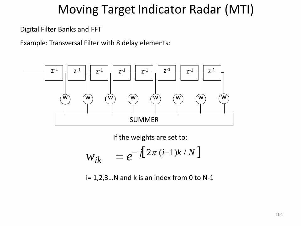
Moving Target Indicator Radar (MTI)
Digital Filter Banks and FFT
Example: Transversal Filter with 8 delay elements:
If the weights are set to:
wik e j2 (i1)k / N
i= 1,2,3…N and k is an index from 0 to N-1
101
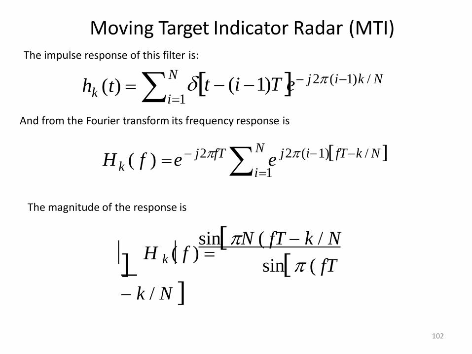
Moving Target Indicator Radar (MTI) The impulse response of this filter is:
k i1 h (t) N
t (i 1)T e j 2 (i1)k / N
And from the Fourier transform its frequency response is
N
k e i1
1)fT k / N H ( f ) e j 2 (i j 2fT
The magnitude of the response is
sinN ( fT k / N
H k ( f )
sin ( fT
k / N
102
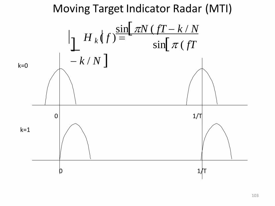
Moving Target Indicator Radar (MTI)
sinN ( fT k / N
H k ( f )
sin ( fT
k / N k=0
0 1/T
0
103
1/T
k=1

Moving Target Indicator Radar (MTI) The response for all eight filters is:
104
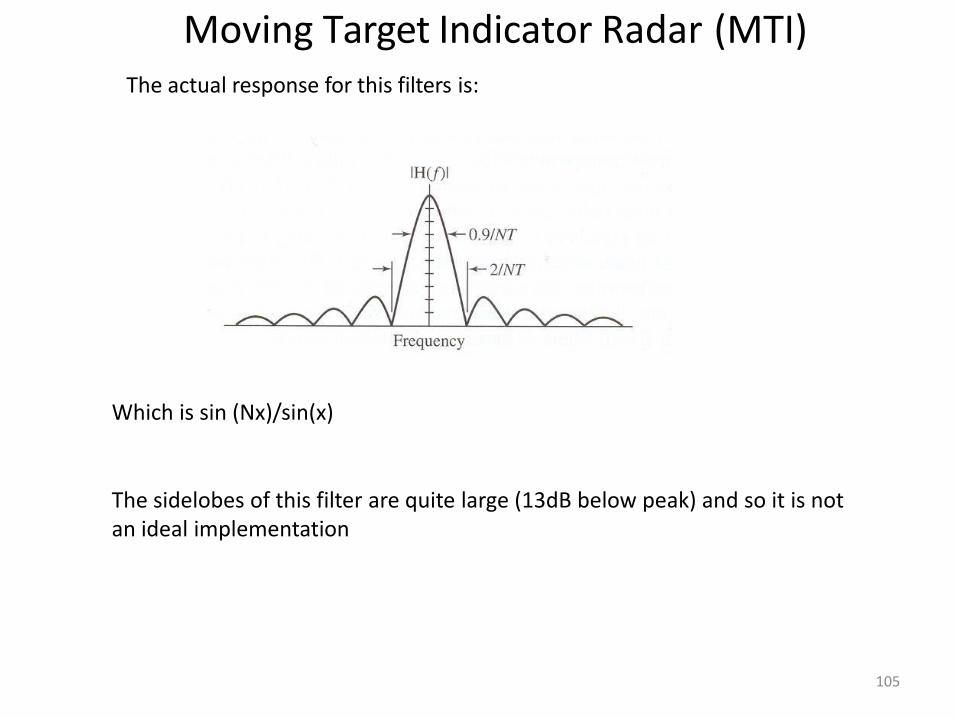
Moving Target Indicator Radar (MTI) The actual response for this filters is:
Which is sin (Nx)/sin(x)
The sidelobes of this filter are quite large (13dB below peak) and so it is not an ideal implementation
105
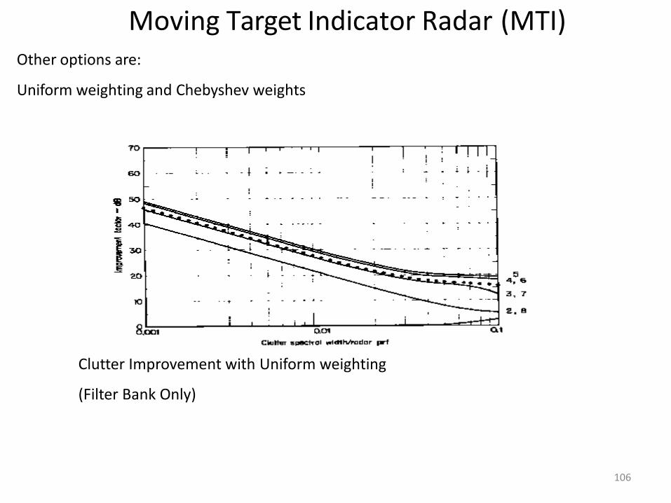
Moving Target Indicator Radar (MTI) Other options are:
Uniform weighting and Chebyshev weights
Clutter Improvement with Uniform weighting
(Filter Bank Only)
106

Moving Target Indicator Radar (MTI)
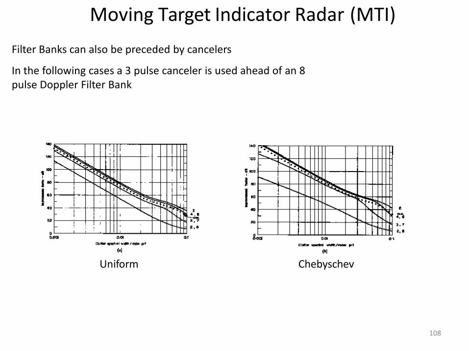
Filter Banks can also be preceded by cancelers
In the following cases a 3 pulse canceler
107
Moving Target Indicator Radar (MTI)
Filter Banks can also be preceded by cancelers
In the following cases a 3 pulse canceler is used ahead of an 8 pulse Doppler Filter Bank
Uniform
108
Chebyschev
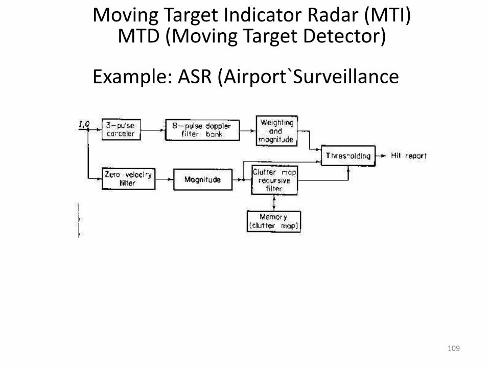
Moving Target Indicator Radar (MTI) MTD (Moving Target Detector)
Example: ASR (Airport`Surveillance Radar)
109
Moving Target Indicator Radar (MTI) MTD (Moving Target
Detector) Example: ASR (Airport`Surveillance Radar)
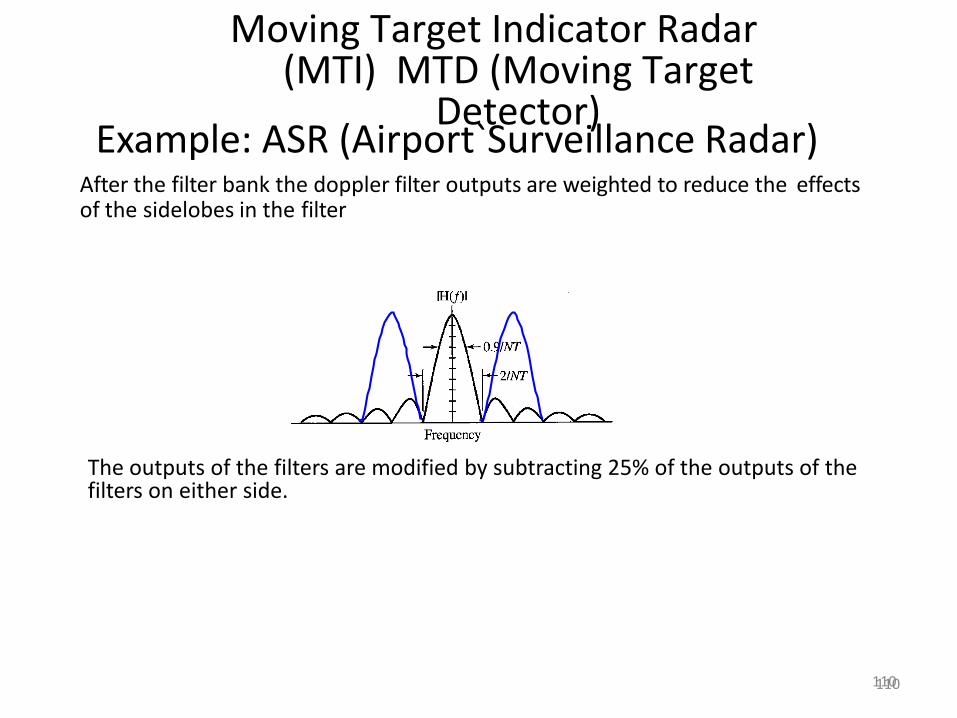
After the filter bank the doppler filter outputs are weighted to reduce the effects of the sidelobes in the filter
110
The outputs of the filters are modified by subtracting 25% of the outputs of the filters on either side.
110

Moving Target Indicator Radar (MTI) MTD (Moving Target Detector)
Example: ASR (Airport`Surveillance Radar)
111
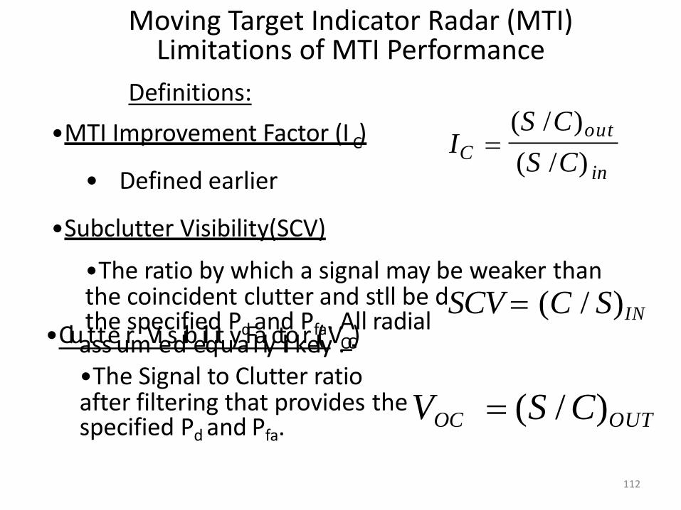
Moving Target Indicator Radar (MTI) Limitations of MTI Performance
Definitions:
C •MTI Improvement Factor (I )
• Defined earlier
•Subclutter Visibility(SCV)
•The ratio by which a signal may be weaker than
the specified Pd and Pfa. All radial etected with
velocities •CluatstseurmViesdibeilqituyaFlalyctliokrel(yV.OC)
•The Signal to Clutter ratio after filtering that provides the VOC (S / C)OUT specified Pd and Pfa.
in
(S / C)out IC
(S / C)
the coincident clutter and stll be dSCV (C / S)IN
112

n
n
Moving Target Indicator Radar (MTI) Limitations of MTI Performance
Definitions:
•Clutter Attenuation
• Defined earlier
•Cancellation Ratio
•The ratio by which a signal may be weaker than the coincident clutter and stll ben detected with the specified Pd and Pfa. All radian l velocities
umed equally likely. •Noatses
CA (CIN / COUT )
C
113
S (SCV )(VOC )
OUT IN
C
C S I

114
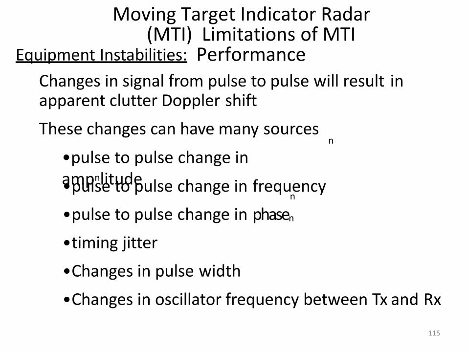
Moving Target Indicator Radar (MTI) Limitations of MTI
Performance Equipment Instabilities:
Changes in signal from pulse to pulse will result in apparent clutter Doppler shift
These changes can have many sources n
•pulse to pulse change in ampnlitude •pulse to pulse change in frequency
n
•pulse to pulse change in phasen
•timing jitter
•Changes in pulse width
•Changes in oscillator frequency between Tx and Rx
115
Moving Target Indicator Radar (MTI) Limitations of MTI
Performance Equipment Instabilities:
Changes in signal from pulse to pulse will result in apparent clutter Doppler shift
These changes can have many sources n
•pulse to pulse change in ampnlitude •pulse to pulse change in frequency
n
•pulse to pulse change in phasen
•timing jitter
•Changes in pulse width
•Changes in oscillator frequency between Tx and Rx
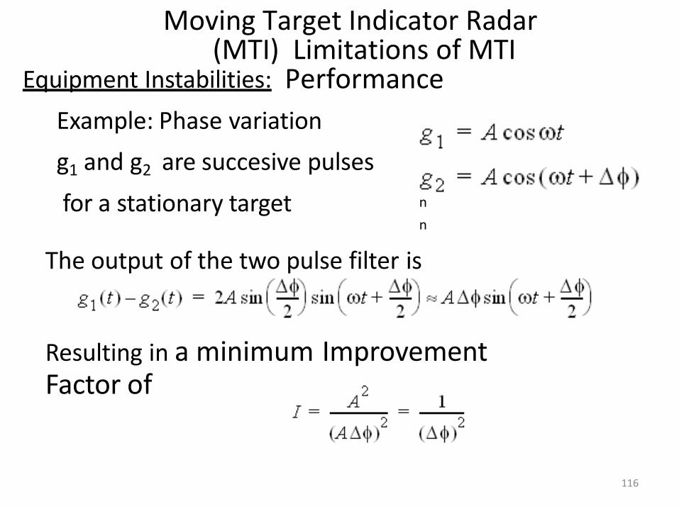
Moving Target Indicator Radar (MTI) Limitations of MTI
Performance
n
n
n
n
Equipment Instabilities:
Example: Phase variation
g1 and g2 are succesive pulses
for a stationary target
The output of the two pulse filter is
Resulting in a minimum Improvement Factor of
116
n
n
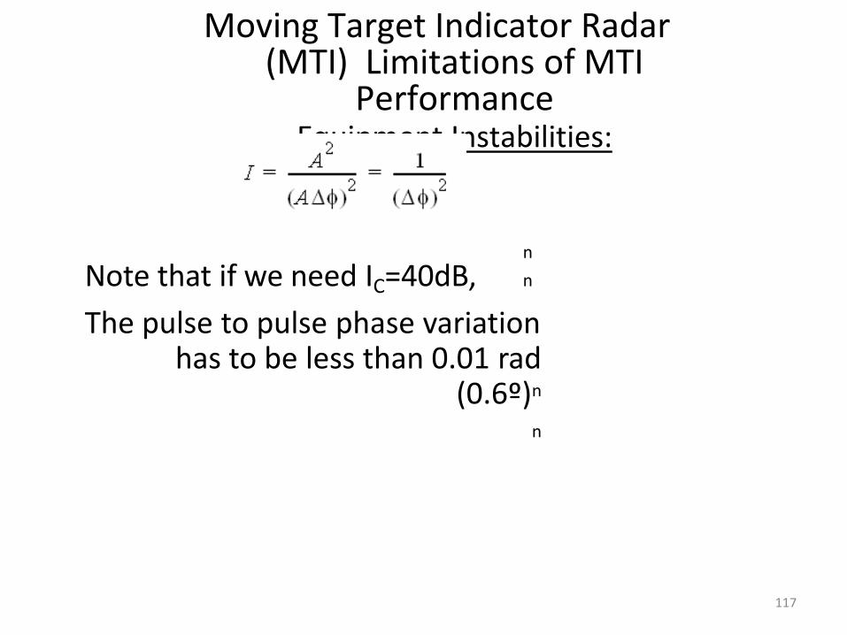
Moving Target Indicator Radar (MTI) Limitations of MTI
Performance Equipment Instabilities:
Note that if we need IC=40dB,
117
The pulse to pulse phase variation has to be less than 0.01 rad
(0.6º)n
n
Moving Target Indicator Radar (MTI) Limitations of MTI
Performance
n
n
n
n
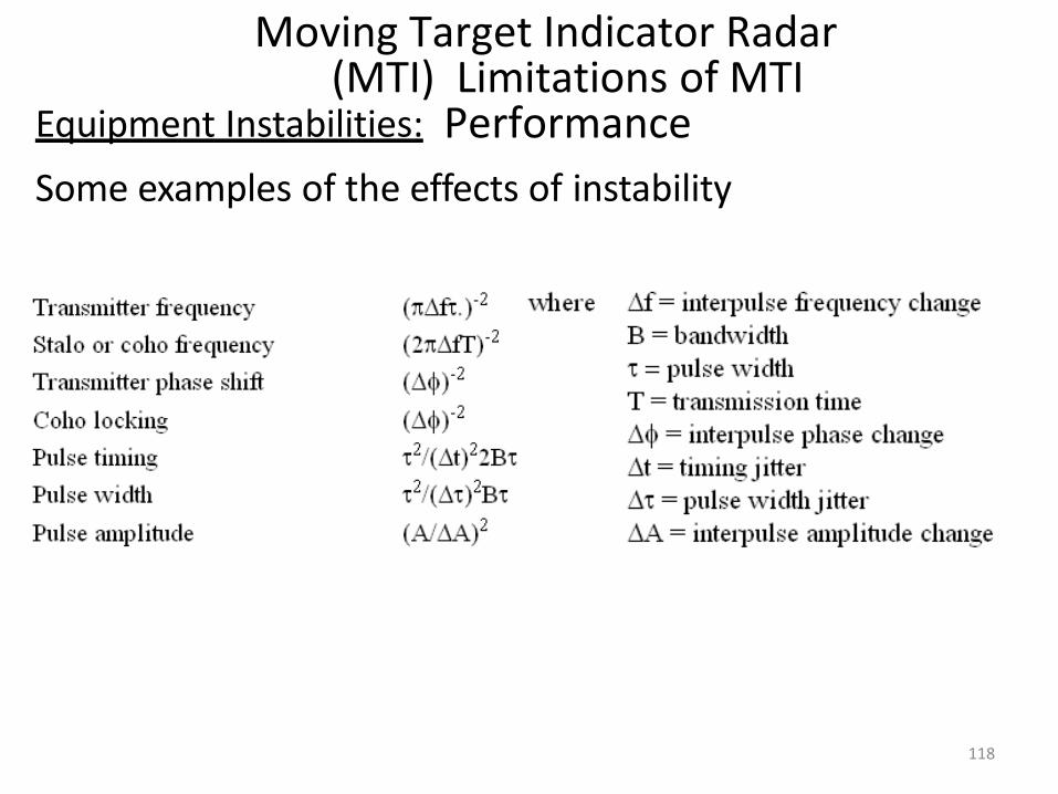
Equipment Instabilities:
Some examples of the effects of instability
118
119
Moving Target Indicator Radar (MTI) Limitations of MTI
Performance
n
n
n
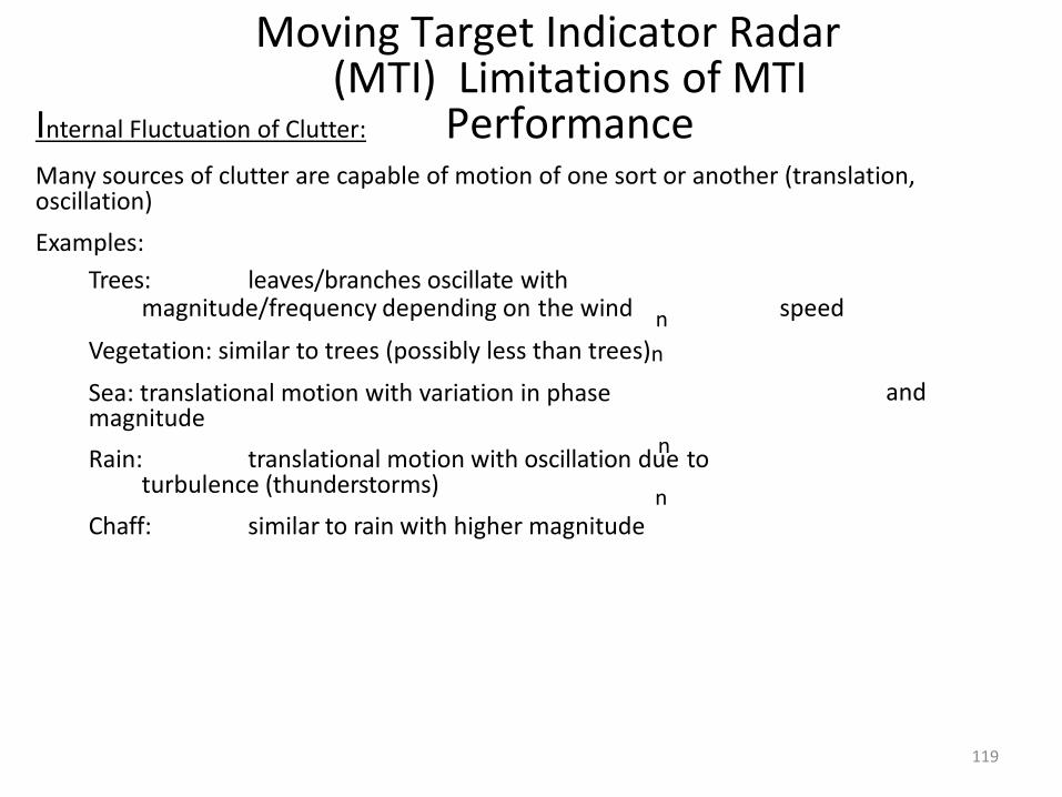
Internal Fluctuation of Clutter:
Many sources of clutter are capable of motion of one sort or another (translation, oscillation)
Examples:
Trees: leaves/branches oscillate with magnitude/frequency depending on the wind speed
and
Vegetation: similar to trees (possibly less than trees)n
Sea: translational motion with variation in phase magnitude
Rain: translational motion with oscillation due to turbulence (thunderstorms)
Chaff: similar to rain with higher magnitude
Moving Target Indicator Radar (MTI) Limitations of MTI
Performance
n
n
n
n
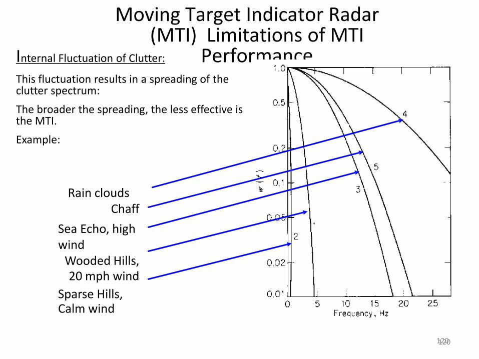
Internal Fluctuation of Clutter:
This fluctuation results in a spreading of the clutter spectrum:
The broader the spreading, the less effective is the MTI.
Example:
Rain clouds Chaff
Sea Echo, high wind
Wooded Hills, 20 mph wind
Sparse Hills, Calm wind
120 120
121
Moving Target Indicator Radar (MTI) Limitations of MTI
Performance
n
n
Internal Fluctuation of Clutter:
The spectrum of clutter can be expressed mathematically as a function of one of three variables:
1. a, a parameter given by Figure 4.29 for various clutter types
2. σC, the RMS clutter frequency spread in Hz
3. σv, the RMS clutter velocity spread in m/s
the clutter power spectrum is represented by W(f) n
n

Moving Target Indicator Radar (MTI) Limitations of MTI
Performance
n
n
n
n
Internal Fluctuation of Clutter:
The power spectra expressed in the three parameters are:
1.
2.
3.
122
Moving Target Indicator Radar (MTI) Limitations of MTI
Performance
n
n
n
n
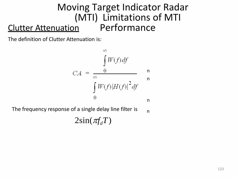
Clutter Attenuation The definition of Clutter Attenuation is:
The frequency response of a single delay line filter is
2sin(fdT )
123
Moving Target Indicator Radar (MTI) Limitations of MTI
Performance
n
n
n
n
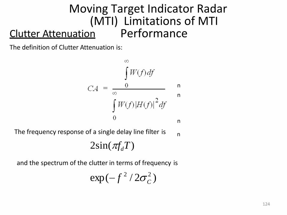
Clutter Attenuation The definition of Clutter Attenuation is:
The frequency response of a single delay line filter is
2sin(fdT )
124
and the spectrum of the clutter in terms of frequency is
2 2
C exp( f / 2 )
Moving Target Indicator Radar (MTI) Limitations of MTI
Performance
n
n
n
n
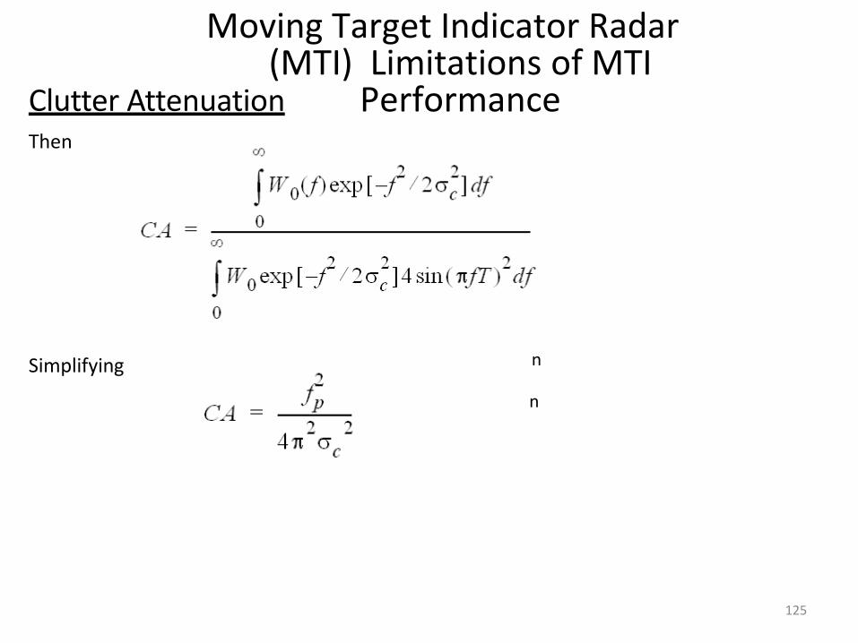
Clutter Attenuation Then
Simplifying
125
Moving Target Indicator Radar (MTI) Limitations of MTI
Performance
n
n
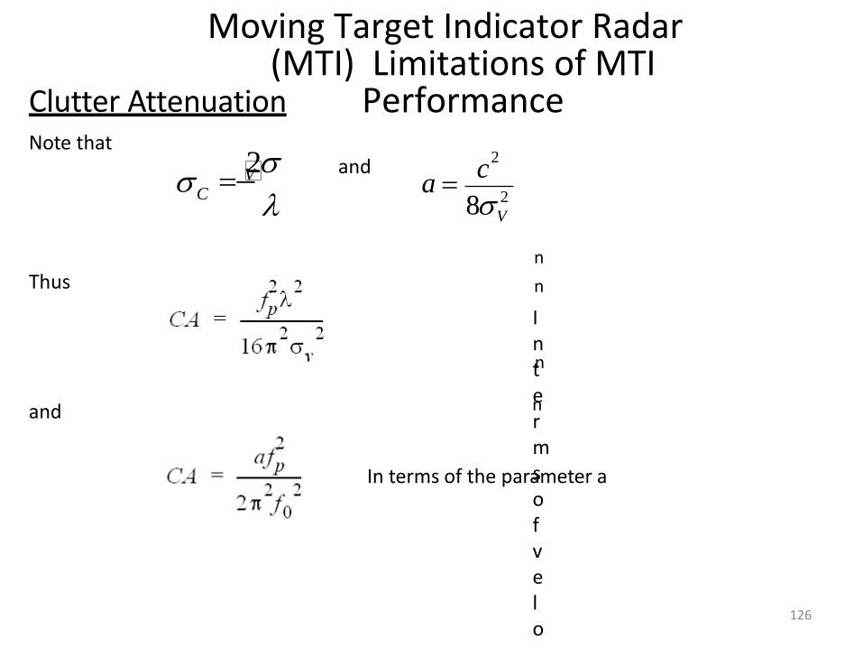
Clutter Attenuation Note that
C
2 V and
2
2
V 8 a
c
Thus
and
n
n
In terms of veloc
126
In terms of the parameter a
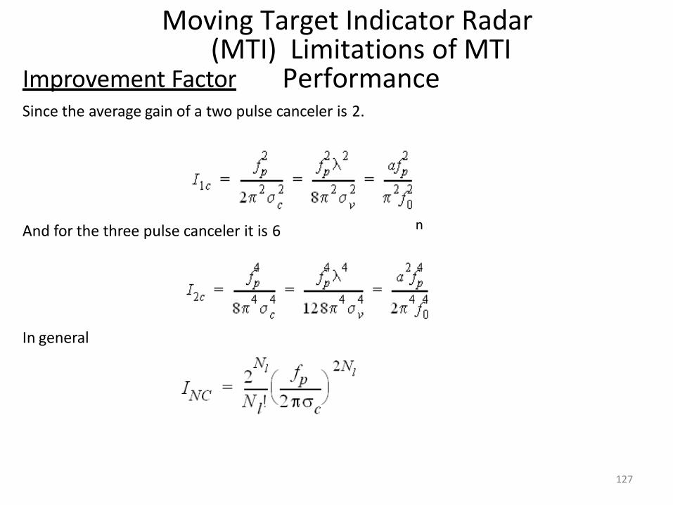
Moving Target Indicator Radar (MTI) Limitations of MTI
Performance
n
n
n
n
Improvement Factor Since the average gain of a two pulse canceler is 2.
And for the three pulse canceler it is 6
In general
127

Moving Target Indicator Radar (MTI) Limitations of MTI
Performance
n
Antenna Scanning Modulation Since the antenna spends only a short time on the target, the spectrum of any target is spread even if the target is perfectly stationary:
The two way voltage antenna pattern is
n n
Dividing numerator and denominator of exponent by the sncan rate
128
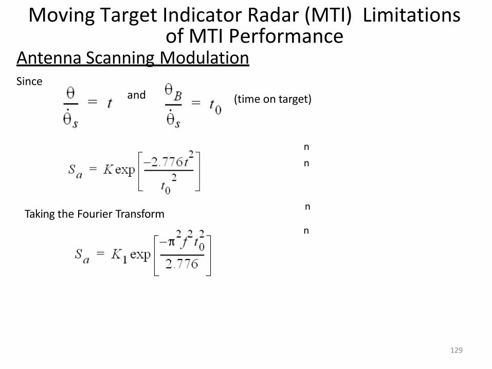
Moving Target Indicator Radar (MTI) Limitations of MTI Performance
n
n
n
n
Antenna Scanning Modulation Since
and (time on target)
Taking the Fourier Transform
129
Moving Target Indicator Radar (MTI) Limitations of MTI Performance
n
n
n
n
f
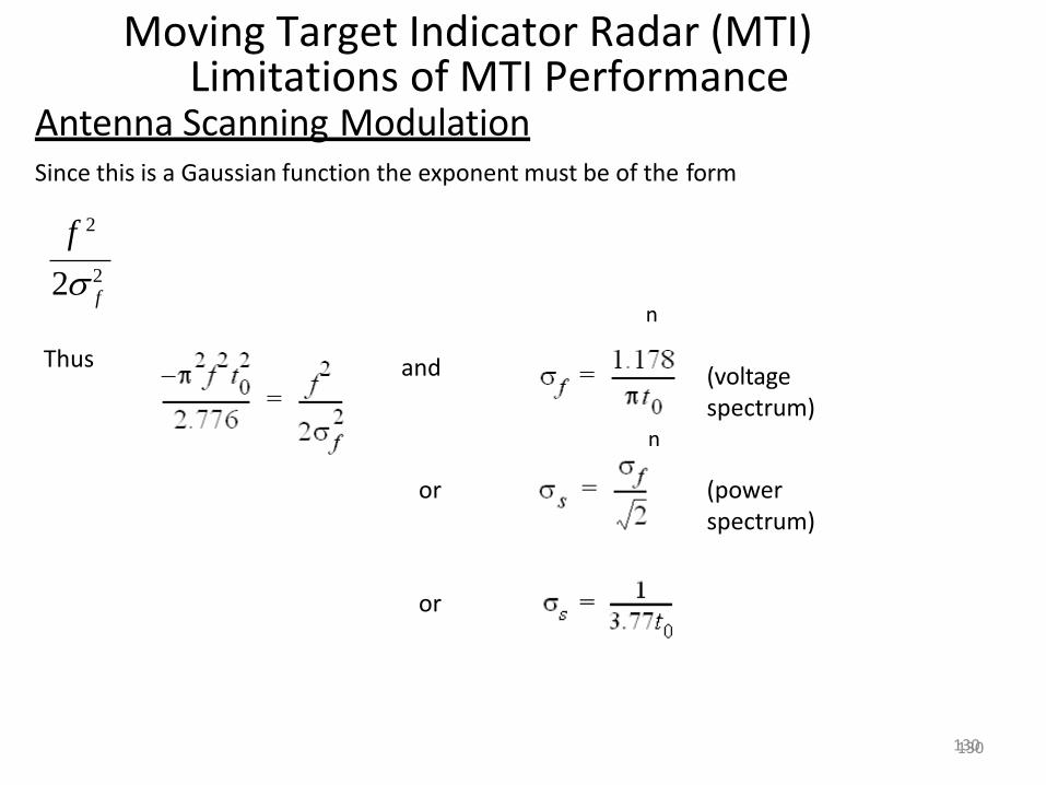
Antenna Scanning Modulation Since this is a Gaussian function the exponent must be of the form
f 2
2 2
Thus and (voltage spectrum)
or (power spectrum)
or
130 130
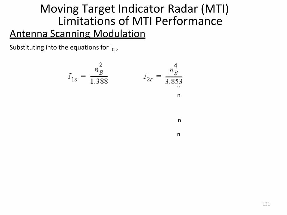
Moving Target Indicator Radar (MTI) Limitations of MTI Performance
n
n
n
n
Antenna Scanning Modulation Substituting into the equations for IC ,
131
132
Tracking with Scanning Radars (Track While scan)
n
n
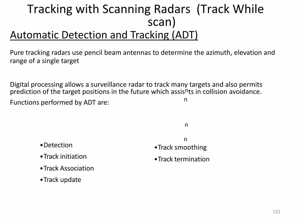
Automatic Detection and Tracking (ADT)
Pure tracking radars use pencil beam antennas to determine the azimuth, elevation and range of a single target Digital processing allows a surveillance radar to track many targets and also permits prediction of the target positions in the future which assisnts in collision avoidance.
Functions performed by ADT are:
•Detection
•Track initiation
•Track Association
•Track update
n
•Track smoothing
•Track termination

Tracking with Scanning Radars (Track While scan)
n
n
Automatic Detection and Tracking (ADT)
Target Detection (Range)
As described before, the range is divided into range cells or “bins” whose dimensions are close to the resolution of the radar.
Each cell has a threshold and if a predetermined number of pulses exceed the threshold a target is declared present
Target Detection (Azimuth)
Resolution better than antenna beamwidth is obtained by seeking the central pulse in the n pulses and using the azimuth associated withnthat pulse.
Thus theoretically the resolution is n
f p
360 6
133
Tracking with Scanning Radars (Track While scan)
n
Automatic Detection and Tracking (ADT)
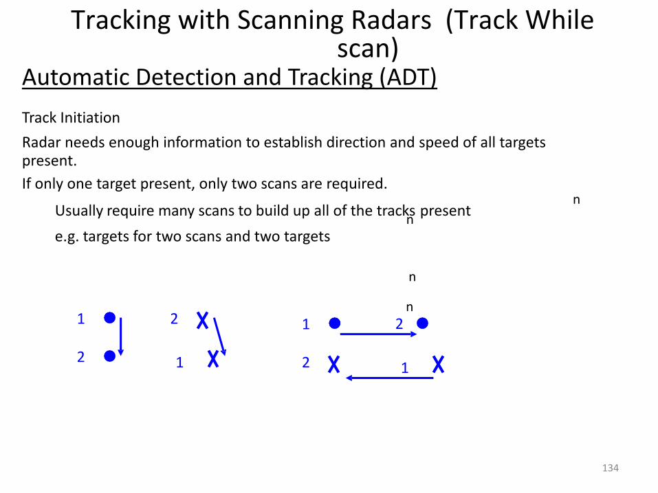
Track Initiation
Radar needs enough information to establish direction and speed of all targets present.
If only one target present, only two scans are required. n
Usually require many scans to build up all of the tracks present
e.g. targets for two scans and two targets
n
1
2
2
1
1
2
n 2
1
134
Tracking with Scanning Radars (Track While scan)
Automatic Detection and Tracking (ADT)
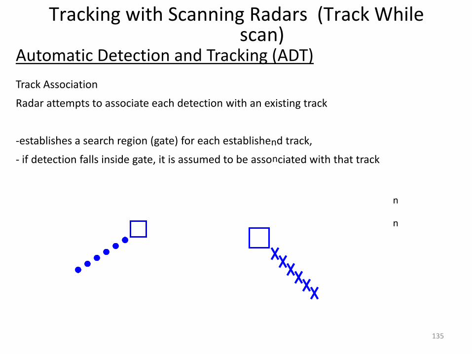
Track Association
Radar attempts to associate each detection with an existing track
-establishes a search region (gate) for each establishend track,
- if detection falls inside gate, it is assumed to be assonciated with that track
n
n
135
Tracking with Scanning Radars (Track While scan)
n
n
Automatic Detection and Tracking (ADT)
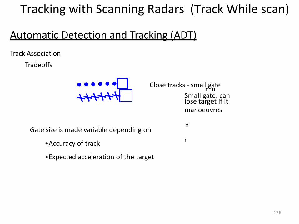
Track Association
Tradeoffs
Close tracks - small gate
136
n n Small gate: can lose target if it manoeuvres
Gate size is made variable depending on
•Accuracy of track
•Expected acceleration of the target
n
n
n
n
Tracking with Scanning Radars (Track While scan)
Automatic Detection and Tracking (ADT)
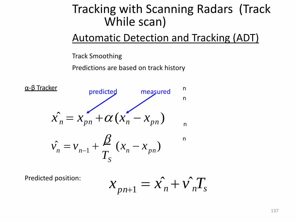
Track Smoothing
Predictions are based on track history
α-β Tracker
x̂ n xpn (xn xpn )
pn n
S
n T
v̂ v n1
(x x )
predicted measured
137
Predicted position: x x̂ n v̂ nTs pn1
UNIT –IV
138
TRACKING RADAR
139
1. Introduction
• Tracking radar systems are used to measure the targets range, azimuth angle, elevation angle, and velocity
• Predict the future values
• Target tracking is important to military and
civilian purposes as missile guidance and airport traffic control
140
Target tracking
Targets are divided to two types:
1 Single target
2 Multiple targets
140

141
Single target
1 Angle tracking A- Sequential lobing B- Conical scan C- Amplitude compression monopulse D- Phase compression monopulse
2 Range tracking
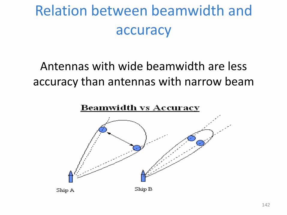
Relation between beamwidth and accuracy
Antennas with wide beamwidth are less accuracy than antennas with narrow beam
142
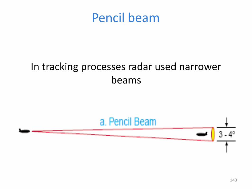
Pencil beam
In tracking processes radar used narrower beams
143
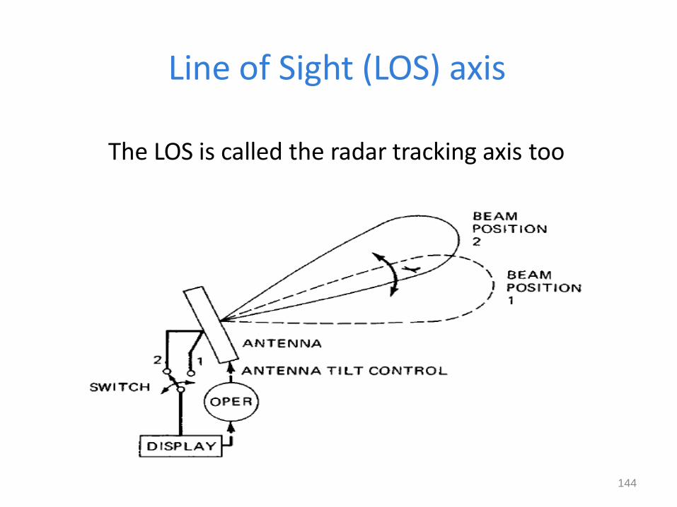
Line of Sight (LOS) axis
The LOS is called the radar tracking axis too
144

145
Error signal
• Describes how much the target has deviated from the beam main axis
• Radar trying to produce a zero error signal
• Azimuth and elevation error
146
1. Sequential lobing
• Sequential lobing is often referred to as lobe switching or sequential switching
• Accuracy depends on the pencil beam width
• It is very simple to implement
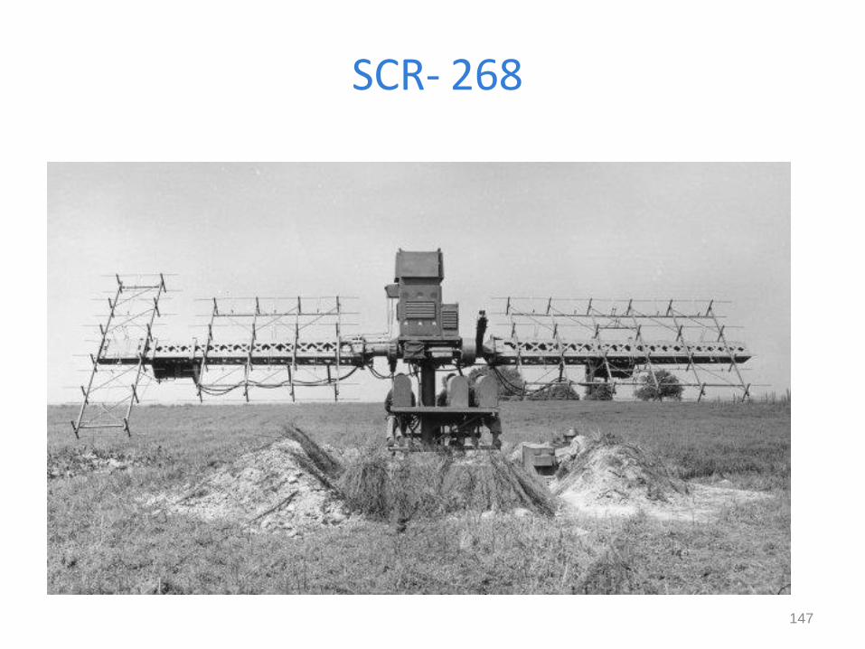
SCR- 268
147
148
Concept of operation:
Measuring the difference between the echo signals voltage levels

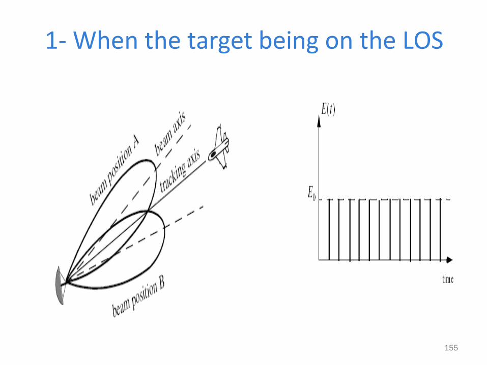
1- When the target being on the LOS
The difference between the echo signals voltage in (A) and (B) equal zero, that’s mean zero error signal
149
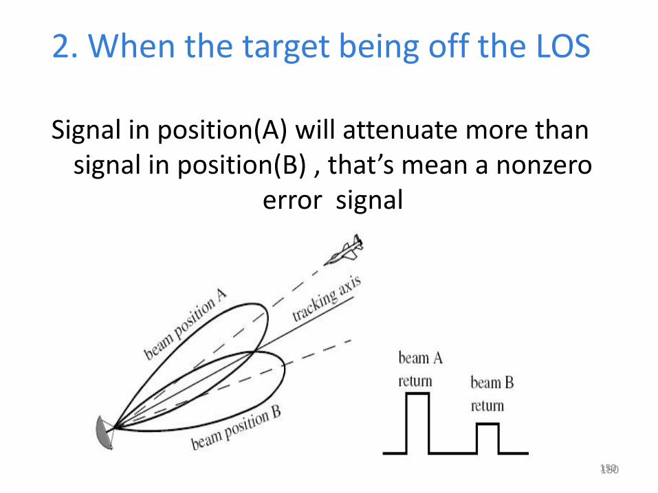
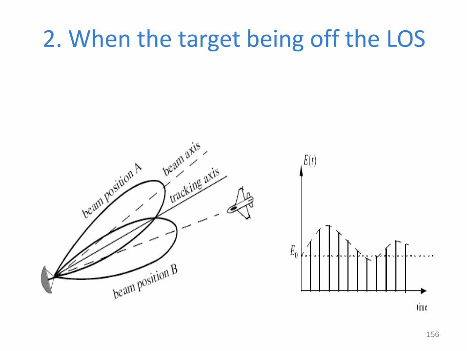
2. When the target being off the LOS
Signal in position(A) will attenuate more than signal in position(B) , that’s mean a nonzero
error signal
150 150

Mat lab Code
151 151

2. Conical scan
- It’s an extension of sequential lobbing
- The feed of antenna is rotating around the antenna axis
152

- The envelope detector is used to extract the return signal amplitude
- AGC is used to reduce the echo signal amplitude if it is strong and raises it when it is weaker
153

Elevation and azimuth error
154
1- When the target being on the LOS
155
2. When the target being off the LOS
156
157
3. Amplitude compression monopulse
• This type is more accurate than sequential and conical scanning
• Feed generated four beams simultaneously
with single pulse
• The four beams are inphase but have different
amplitudes.
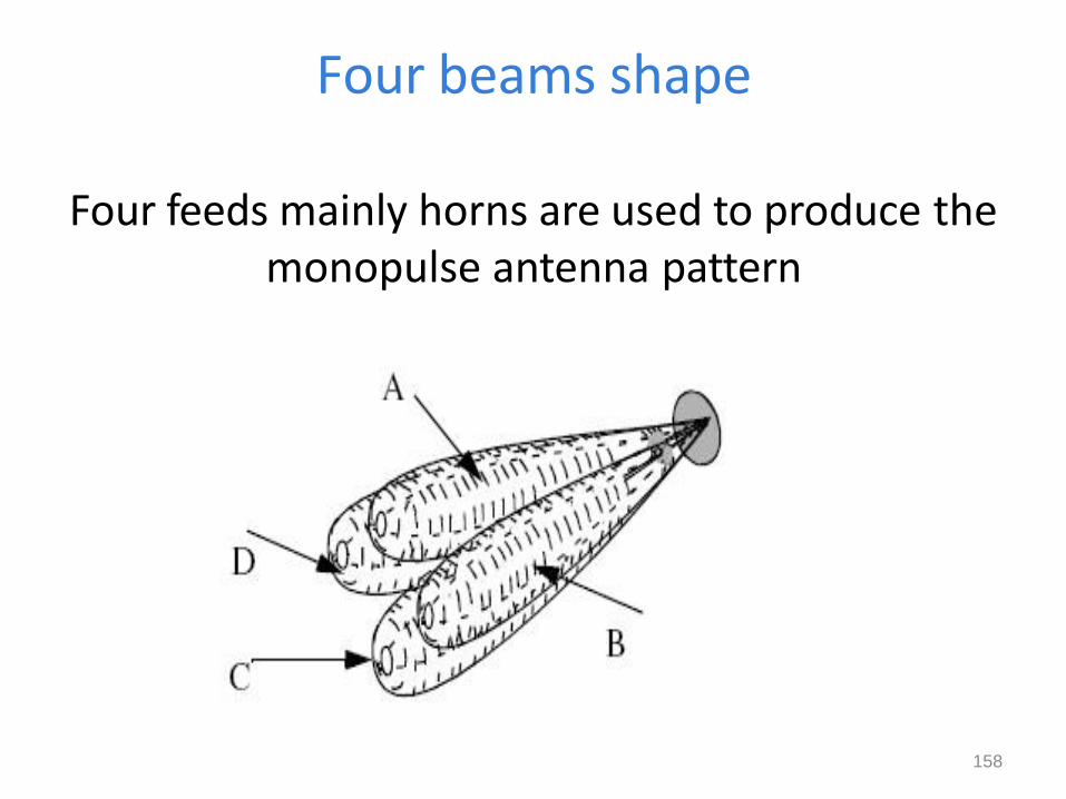
Four beams shape
Four feeds mainly horns are used to produce the monopulse antenna pattern
158

Simplified amplitude comparison monopulse radar block diagram
159

When the target being on the LOS
radar compares the amplitudes and phases of all echo signals of target
160 160
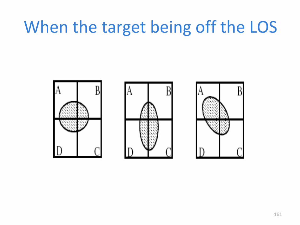
When the target being off the LOS
161
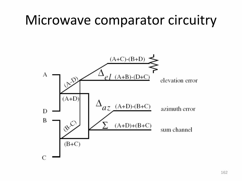
Microwave comparator circuitry
162
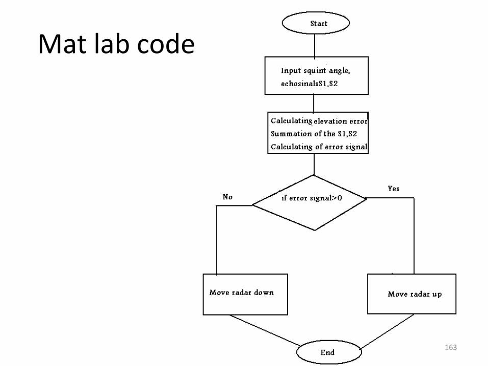
Mat lab code
163 163
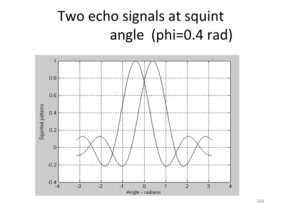
Two echo signals at squint angle (phi=0.4 rad)
164
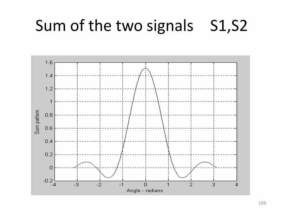
Sum of the two signals S1,S2
165

Difference between S1,S2
166

Elevation Error signal
167
168
4- Phased compression monopulse
• It’s the same as the last type but the amplitude here is equal for the four beams with different phases
• Phase comparison monopulse tracking radars use a minimum of a two-element array antenna
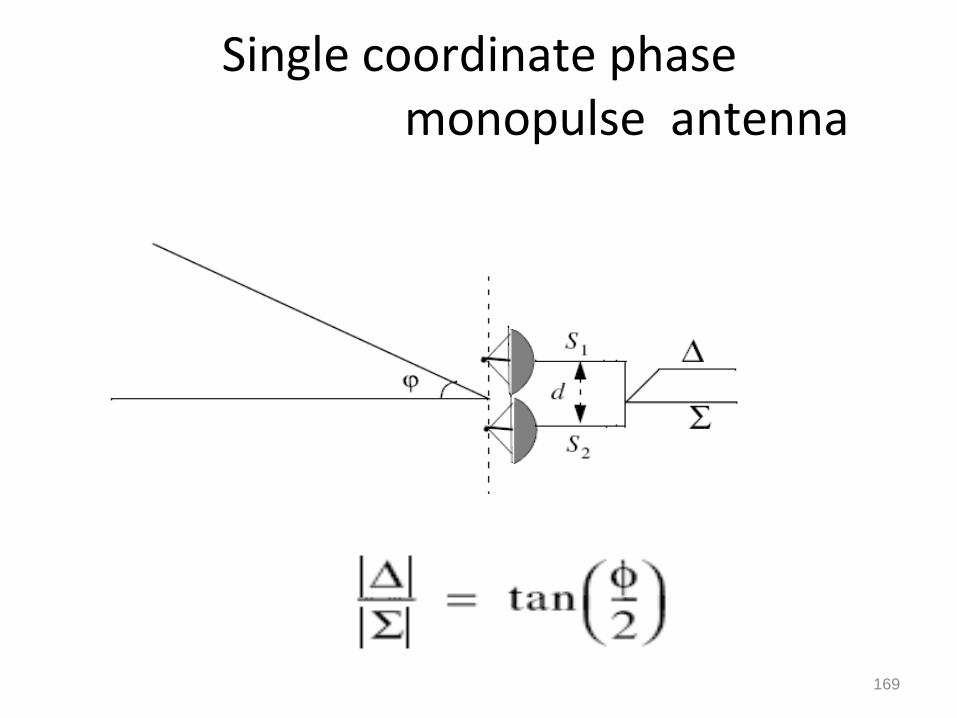
Single coordinate phase monopulse antenna
169
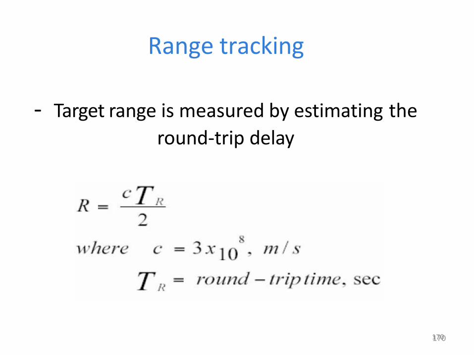
Range tracking
- Target range is measured by estimating the
round-trip delay
170 170
171
Split Gate System
• It consist of two gates:
1-Early gate 2- Late gate
• The early gate produces positive voltage output but the late gate produces negative voltage output.
• Subtracting & integration
• Output is: zero, negative or positive
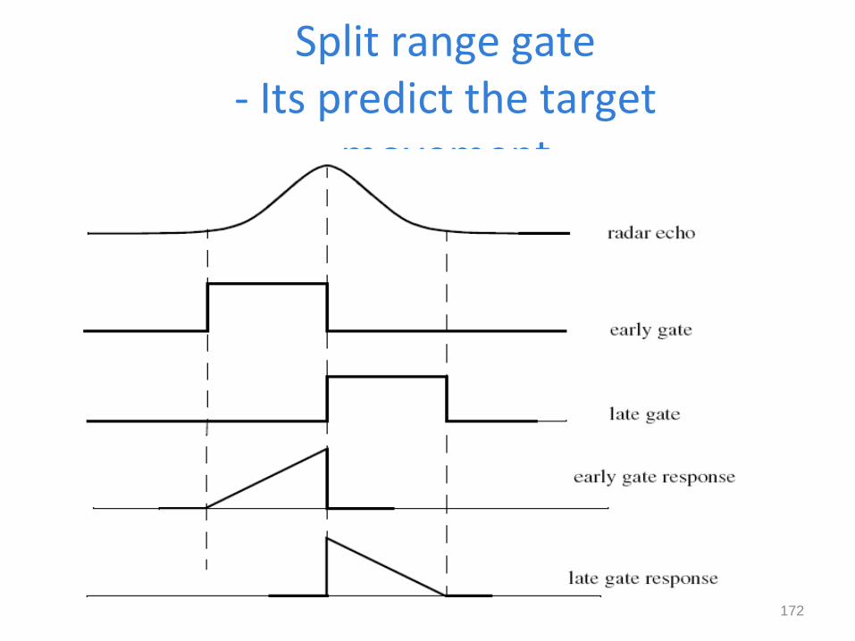
Split range gate - Its predict the target
movement
172
174
Multiple Targets
Here the system is more difficult since:
• Tracking
• Scanning
• reporting

175
Track while scanning (TWS)
• This type of radar is used for multiple targets
• It scans for new targets while its tracking old targets
• When TWS scan a new target it initiates a new
track file
176
177
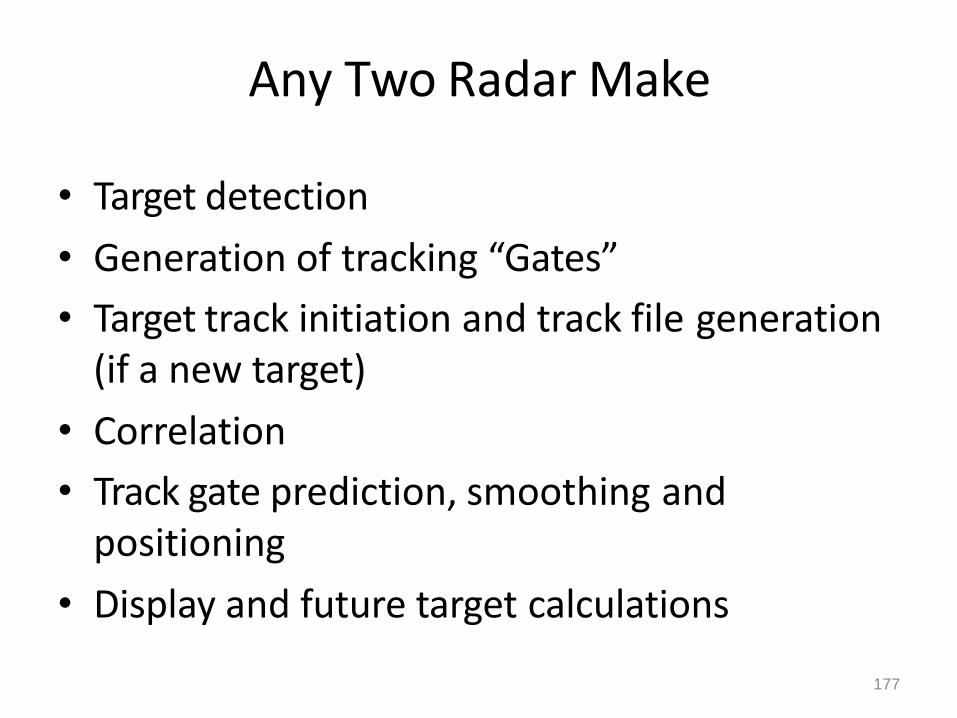
Any Two Radar Make
• Target detection
• Generation of tracking “Gates”
• Target track initiation and track file generation (if a new target)
• Correlation
• Track gate prediction, smoothing and positioning
• Display and future target calculations
178
Target Detection
This task is accomplished by two method :
• Circuit in receiver
• signal-processing equipment
179
Generation Gate
• Gate : small volume of space consist of many of cells
• Function : monitoring of each scan of the
target information
• Gating has responsibility for knowing if new/exist target

180
Gate Types
• Acquisition gate
• Tracking gate
• Turning gate
179

Acquisition Gate
• This gate is large to facilitate target motion cross one scan period
181
182
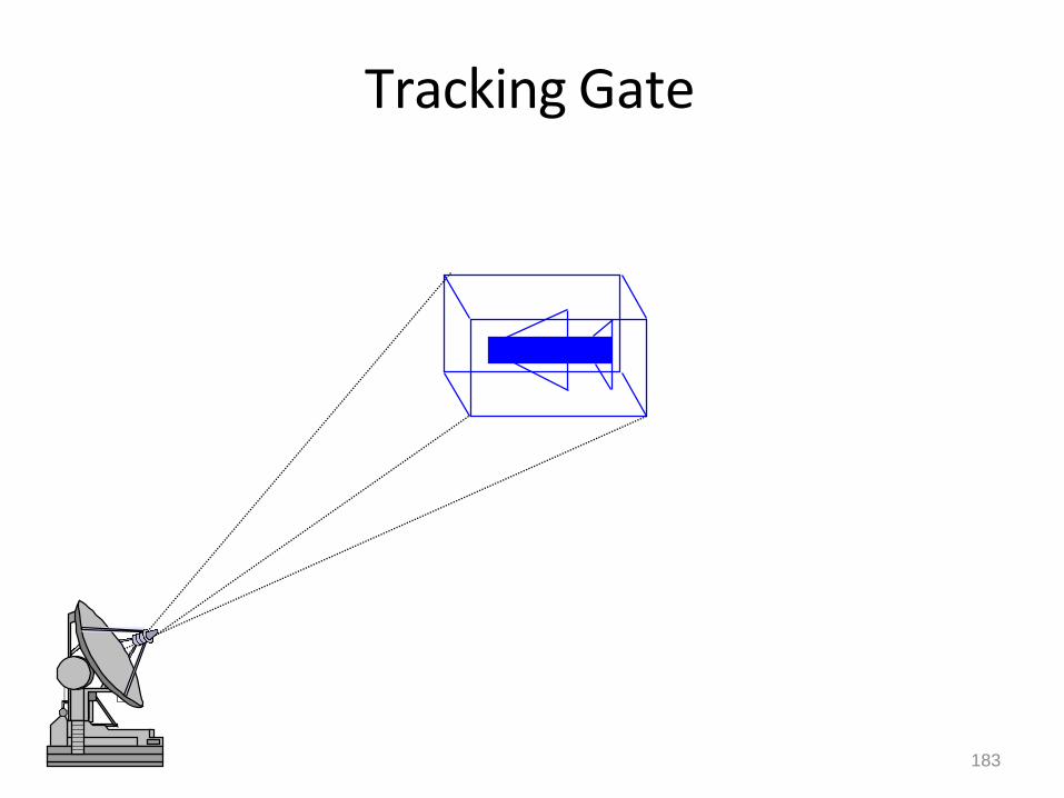
Tracking Gate
• This gate is generated when the target is within the acquisition gate on the next scan
• It is very small gate
• It is moving to the new expected target
position
Tracking Gate
183

184
Turning gate
• It is generated if the observation within the
tracking gate doesn’t appear
• It has larger size than tracking gate
• Tracking gate included by it
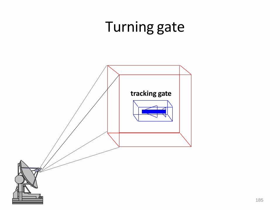
Turning gate
tracking gate
185

186
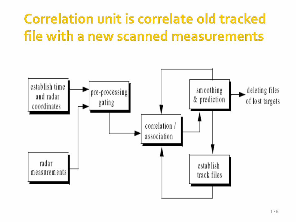
Target track correlation and association
• All observations site on the boundary of tracking gate must be correlate with that track
• Each observation is compared with all track
files
• Perhaps, observation is correlated with one
track files ,several tracks or no tracks
187
Tracking Ambiguity Results
• If the observation correlates with more one track files, tracking ambiguity is appear.
• Two reasons cause this result:
1 several targets site in the same gate
2 several gates overlap on a single target

188
How To Solve Ambiguity?
• If the system designed so that an operator initiate the tracks, then solution by delete
track
• But for the automatic systems , the solving
by maintain software rules
189
Target track initiation and track file generation
• The track file is initiated when acquisition gate is generated
• Track file store position and gate data
• Each track file occupies position in the digital
computer's high-speed memory
• Cont. refreshed data

Track gate prediction, smoothing and positioning
- Error Repositioning Smoothing
- The system lagged the target
- The system leading the target
- smoothing is completed by comparing
predicted parameters with observed parameters
190 189

TWS System Operation
Scanning radar
detects a target
Do
parameters match those
from previous
scan
Yes Does track
ambiguity
exist
NO
Yes
NO
Genera
te a
new
track
file &
store
data
Generate an
acquisition
gate
Resolve
ambiguity
Target
previously in track
or acquisition
Compute
target tracking
parameters
Acquisition
Track
Generate Track
Gate & indicator in
file
Update
tracking
parameters
Reposition track
gate centered on
future position
Ready for the
next radar scan
information
Recompute
track gate
191
192
Conclusion
• We discussed the concepts of the different ways to determine the angle of a target and its range
• We show the different between single and
multiple targets tracking
• We try to apply that on Matlab .
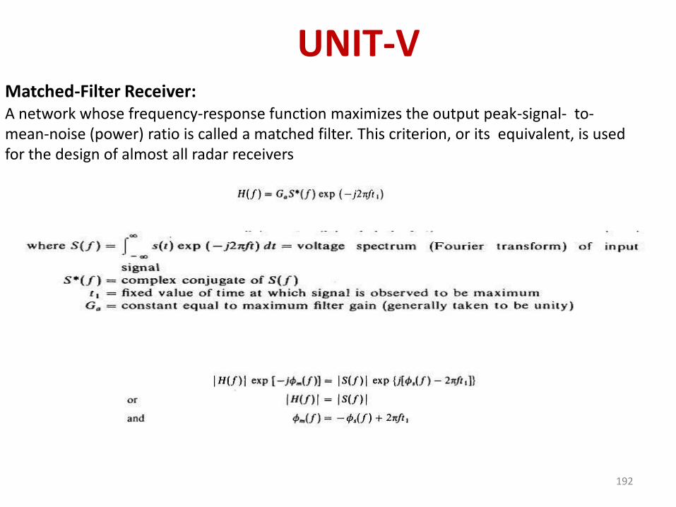
Matched-Filter Receiver: A network whose frequency-response function maximizes the output peak-signal- to- mean-noise (power) ratio is called a matched filter. This criterion, or its equivalent, is used for the design of almost all radar receivers
UNIT-V
192
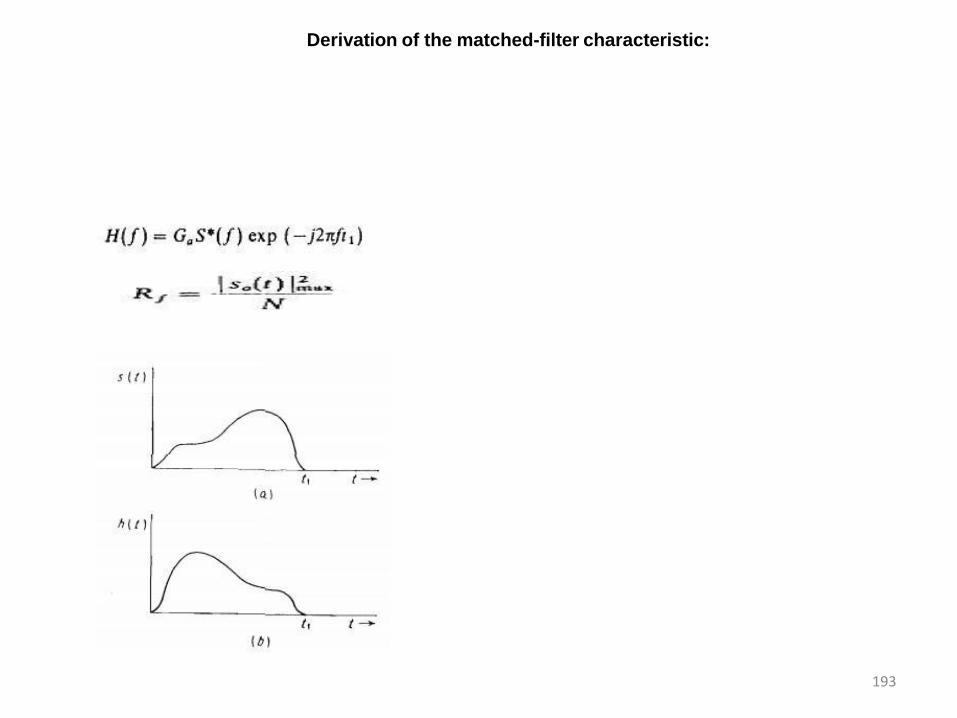
Derivation of the matched-filter characteristic:
193
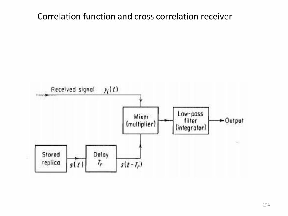
Correlation function and cross correlation receiver
194

EFFICIENCY OF NON-MATCHED FILTERS
195

196
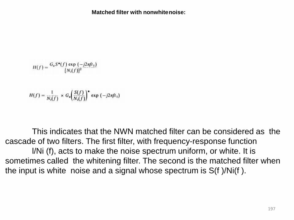
Matched filter with nonwhite noise:
This indicates that the NWN matched filter can be considered as the
cascade of two filters. The first filter, with frequency-response function
l/Ni (f), acts to make the noise spectrum uniform, or white. It is
sometimes called the whitening filter. The second is the matched filter when
the input is white noise and a signal whose spectrum is S(f )/Ni(f ).
197
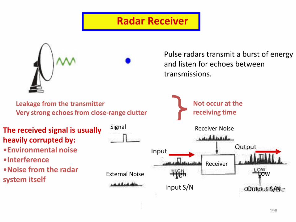
Pulse radars transmit a burst of energy and listen for echoes between transmissions.
Leakage from the transmitter Very strong echoes from close-range clutter
Radar Receiver
The received signal is usually heavily corrupted by: •Environmental noise •Interference •Noise from the radar system itself
Not occur at the receiving time
Input Output
External Noise
Signal Receiver Noise
Receiver
Low
Output S/N
High
Input S/N
198
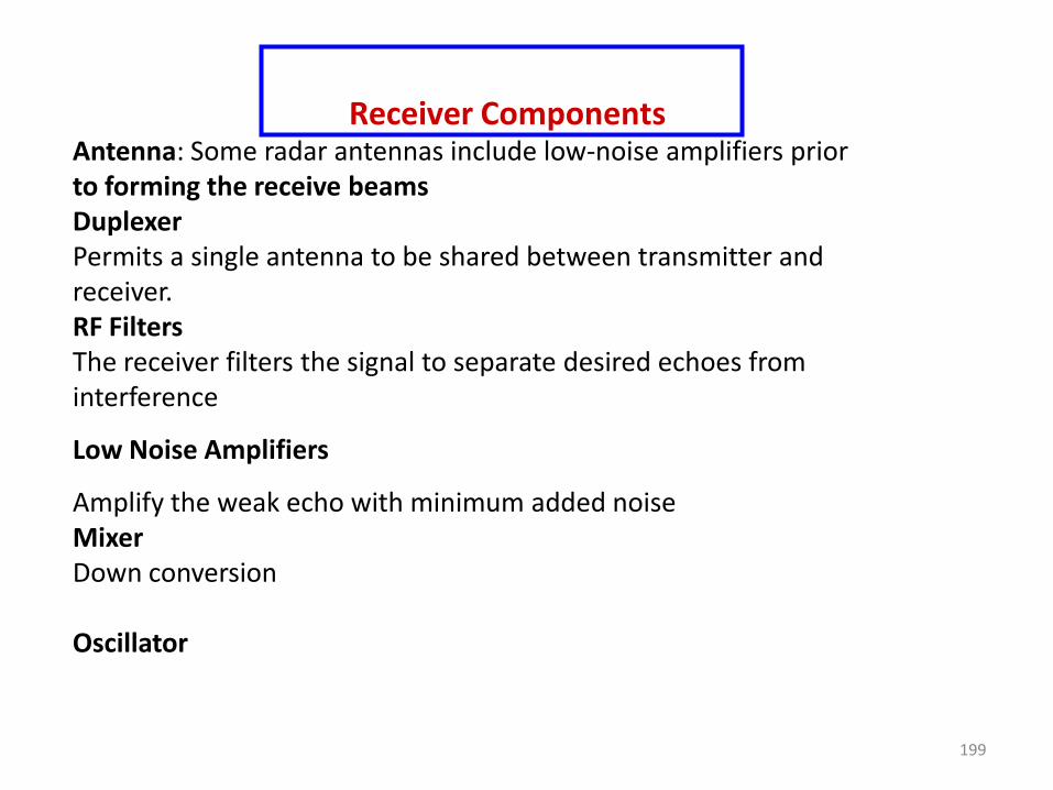
Receiver Components
Antenna: Some radar antennas include low-noise amplifiers prior to forming the receive beams Duplexer Permits a single antenna to be shared between transmitter and receiver. RF Filters The receiver filters the signal to separate desired echoes from interference
Low Noise Amplifiers
Amplify the weak echo with minimum added noise Mixer Down conversion
Oscillator
199
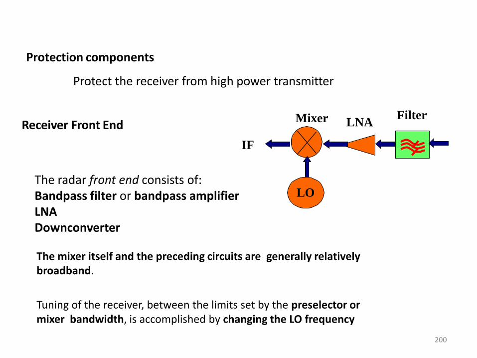
The radar front end consists of: Bandpass filter or bandpass amplifier LNA Downconverter
Receiver Front End
Protection components
Protect the receiver from high power transmitter
The mixer itself and the preceding circuits are generally relatively broadband.
Tuning of the receiver, between the limits set by the preselector or mixer bandwidth, is accomplished by changing the LO frequency
LNA Mixer
LO
Filter
IF
200
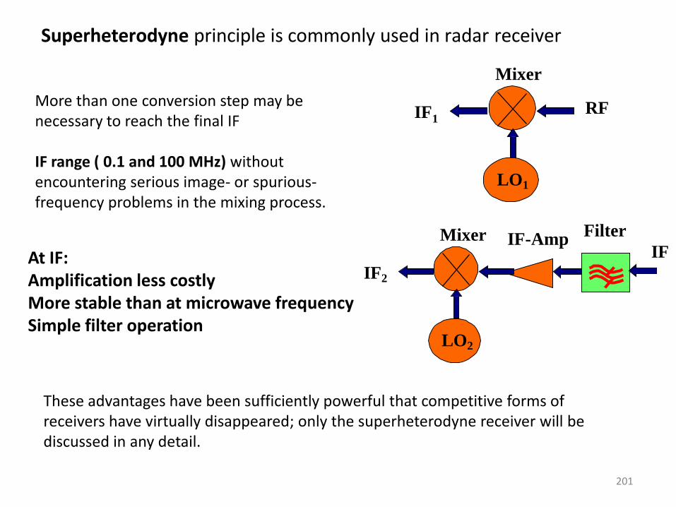
At IF: Amplification less costly More stable than at microwave frequency Simple filter operation
Superheterodyne principle is commonly used in radar receiver
More than one conversion step may be necessary to reach the final IF
IF range ( 0.1 and 100 MHz) without encountering serious image- or spurious- frequency problems in the mixing process.
Mixer
LO1
IF 1 RF
These advantages have been sufficiently powerful that competitive forms of receivers have virtually disappeared; only the superheterodyne receiver will be discussed in any detail.
IF IF-Amp Mixer
LO2
Filter
IF2
201

The function of a radar receiver is to amplify the echoes of the radar transmission and to filter them in a manner that will provide the maximum discrimination between desired echoes and undesired interference.
The interference comprises:
•Energy received from galactic sources •Energy received from neighboring radars •Energy received from neighboring communication systems •Energy received from possibly jammers •Noise generated in the radar receiver •The portion of the radar's own radiated energy that is scattered by undesired targets (such as rain, snow, birds, and atmospheric perturbations)
Receiver Function
202
In airborne radars are used for altimeters or mapping:
• Ground is the desired target
• Other aircraft are undesired targets
More commonly, radars are intended for detection of • Aircraft • Ships • Surface vehicles
203

Noise and Dynamic Range Considerations
Receivers generate internal noise which masks weak echoes being received from the radar transmissions. This noise is one of the fundamental limitations on the radar range
The receiver is often the most critical component
The purpose of a receiver is reliably recovering the desired echoes from a wide spectrum of transmitting sources, interference and noise
Noiseis added into an RF or IF passband and degrades system sensitivity
Receiver should not be overloaded by strong signals
Noise
(So/No)min
Receiver To demodulator
Desired echo + Noise
Internal Noise
Desired echo
204
Noise ultimately determines the threshold for the minimum echo level that can be reliably detected by a receiver.
The receiving system does not register the difference between signal power and noise power. The external source, an antenna, will deliver both signal power and noise power to receiver. The system will add noise of its own to the input signal, then amplify the total package by the power gain
Noise behaves just like any other signal a system processes
Filters:
Attenuators:
will filter noise
will attenuate noise
Noise Effects
205

Thermal Noise
R
The most basic type of noise being caused by thermal vibration of bound charges. Also known as Johnson or Nyquist noise.
R
T
Available noise power
Vn = 4KTBR
Pn = KTB
Where, K = Boltzmann’s constant (1.3810-23J/K)
T Absolute temperature in degrees Kelvin
B IF Band width in Hz
At room temperature 290 K:
For 1 Hz band width,
For 1 MHz Bandwidth
Pn = -174 dBm
Pn = -114 dBm 206

Shot Noise:
Source: random motion of charge carriers in electron tubes or solid state devices.
Noise in this case will be properly analyzed on based on noise figure or equivalent noise temperature Generation-recombination noise:
Recombination noise is the random generation and recombination of holes and electrons inside the active devices due to thermal effects. When a hole and electron combine, they create a small current spike.
207
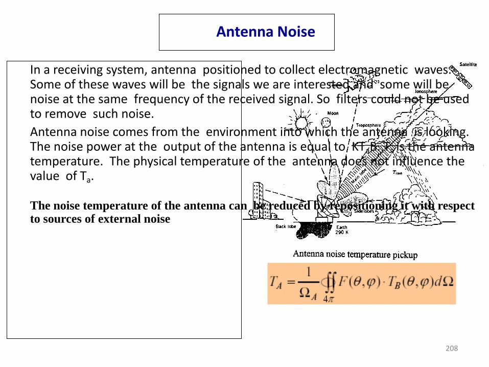
Antenna Noise
In a receiving system, antenna positioned to collect electromagnetic waves. Some of these waves will be the signals we are interested and some will be noise at the same frequency of the received signal. So filters could not be used to remove such noise.
Antenna noise comes from the environment into which the antenna is looking. The noise power at the output of the antenna is equal to KTaB. Ta is the antenna temperature. The physical temperature of the antenna does not influence the value of Ta. The noise temperature of the antenna can be reduced by repositioning it with respect to sources of external noise
208
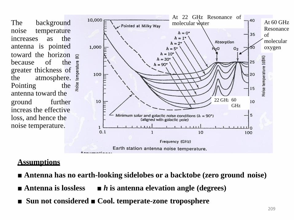
Assumptions
■ Antenna has no earth-looking sidelobes or a backtobe (zero ground noise)
■ Antenna is lossless ■ h is antenna elevation angle (degrees)
■ Sun not considered ■ Cool. temperate-zone troposphere
The background noise temperature increases as the antenna is pointed
toward the horizon because of the greater thickness of the atmosphere. Pointing the antenna toward the
ground further increas the effective loss, and hence the noise temperature.
At 22 GHz Resonance of molecular water At 60 GHz
Resonance of molecular oxygen
22 G Hz 60
GHz
209

Equivalent Noise Temperature and Noise Figure
F = (S/N)i/(S/N)o
Ni = Noise power from a matched load at To = 290 K; Ni
= KTo B.
F is usually expressed in dB
F(dB)=10 log F.
Noise Figure (F)
Two-port
Network Si + Ni So + No
210
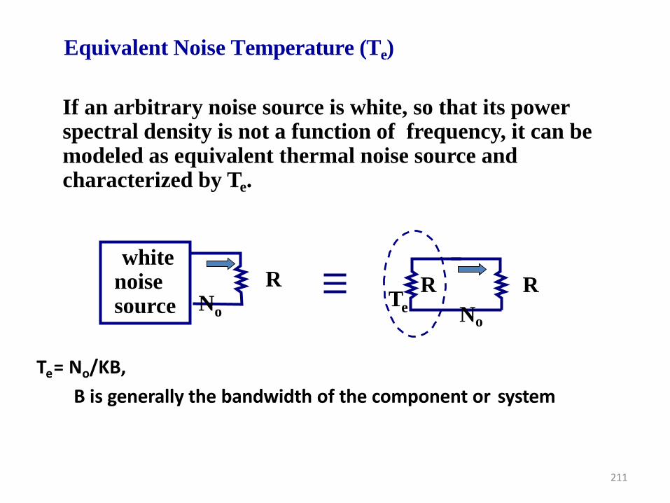
Te = No/KB,
B is generally the bandwidth of the component or system
R N o
white noise source
R R T e No
Equivalent Noise Temperature (Te)
If an arbitrary noise source is white, so that its power spectral density is not a function of frequency, it can be modeled as equivalent thermal noise source and characterized by Te.
211
R
No
G
Noisy amplifier
T = 0
R R
No-int= GKTeB
G
Noiseless amplifier
R
No-int
GKB e T =
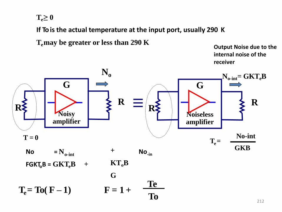
Te ≥ 0
If To is the actual temperature at the input port, usually 290 K
Te may be greater or less than 290 K
Te = To( F – 1) F = 1 + Te
To
Output Noise due to the internal noise of the receiver
No = N o-int No -in
FGKToB = GKTeB +
+
KToB
G
212

Noise Figure of Cascaded Components
Te = To (F - 1)
Ts = Ta + Te Pn = KTsBG,
where, G is the overall gain of the system = G1×G2×G3……×Gn
F2 – 1
G 1 G G 1 2
Fn – 1
G1 G2 ….. Gn-1 T 1 F = F +
F3 – 1 + + …… +
F1
G1
F2
G2
FN-1
GN-1
FN
GN
213
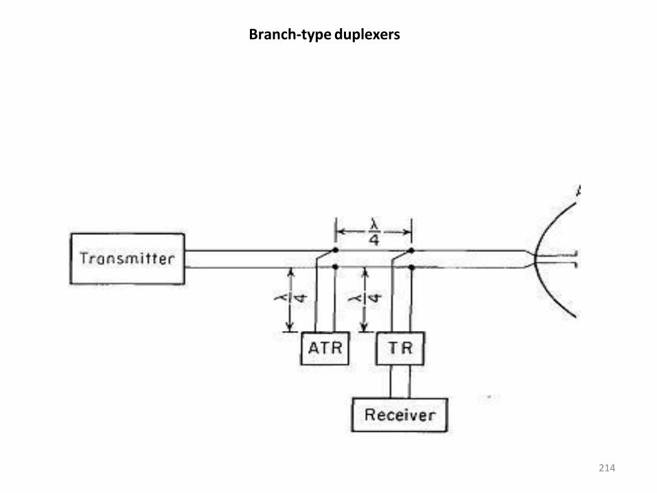
Branch-type duplexers
214
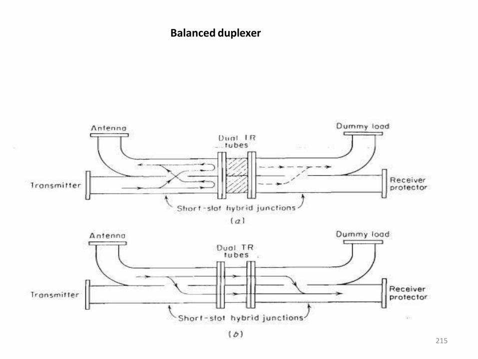
Balanced duplexer
215
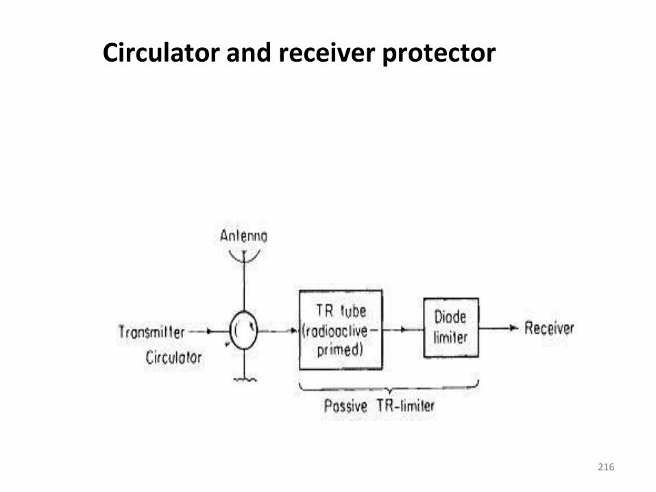
Circulator and receiver protector
216
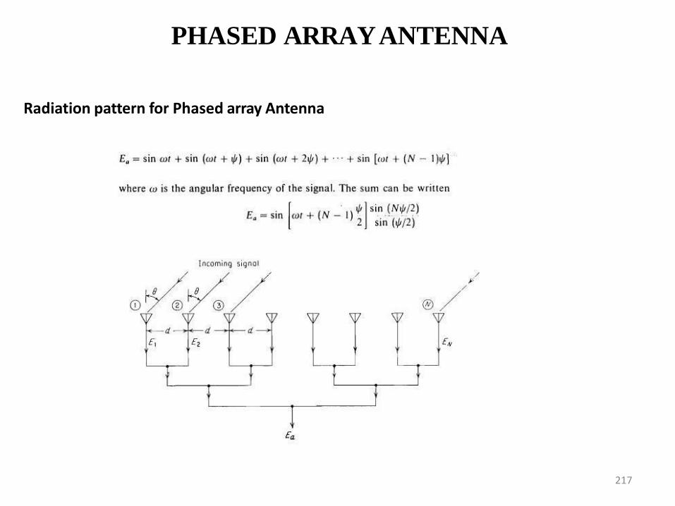
PHASED ARRAY ANTENNA
Radiation pattern for Phased array Antenna
217
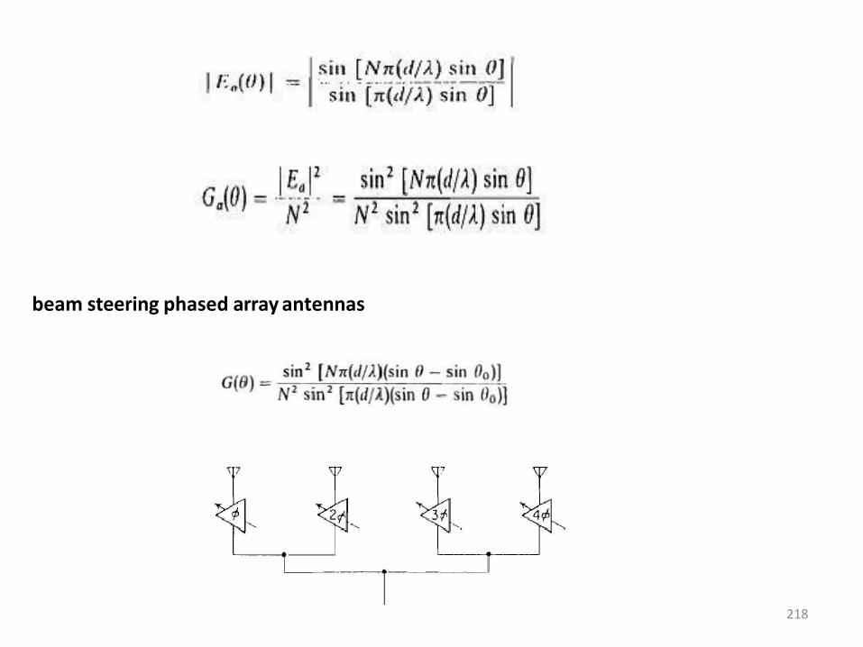
beam steering phased array antennas
218

Applications of phased array antennas
Linear array with frequency scan
Linear array with phase scan:
Phase-frequency planar array:
Phase-phase planar array
219
ADVANTAGES AND LIMITATIONS OF PHASED ARRAY ANTENNAS.
Limitations:
•The major limitation that has limited the widespread use of the conventional phased array in radar is its high cost, which is due in large part to its complexity. •When graceful degradation has gone too far a separate maintenance is needed. •When a planar array is electronically scanned, the change of mutual coupling that accompanies a change in beam position makes the maintenance of low side lobes more difficult. •Although the array has the potential for radiating large power, it is seldom that an array is required to radiate more power than can be radiated by other antenna types or to utilize a total power which cannot possibly be generated by current high- power microwave tube technology that feeds a single transmission line.
220