On maximum entropy regularization for aspecific inverse problem of option pricing

Bernd Hofmann ∗ and Romy Krämer †

Faculty of Mathematics, Technical University ChemnitzD–09107 Chemnitz, Germany

MSC2000 classification scheme numbers: 65J20, 47H30, 49N45, 47B07, 91B28

Abstract

We investigate the applicability of the method of maximum entropy regular-ization (MER) to a specific nonlinear ill-posed inverse problem (SIP) in a purelytime-dependent model of option pricing, introduced and analyzed for an L2-settingin [9]. In order to include the identification of volatility functions with a weak pole,we extend the results of [12] and [13], concerning convergence and convergence ratesof regularized solutions in L1, in some details. Numerical case studies illustrate thechances and limitations of (MER) versus Tikhonov regularization (TR) for smoothsolutions and solutions with a sharp peak. A particular paragraph is devoted tothe singular case of at-the-money options, where derivatives of the forward operatordegenerate.

1 Introduction

In this paper, we are dealt with a specific ill-posed nonlinear inverse problem that arisesin financial markets (for an overview of such problems see [3]). The problem consists infinding (calibrating) a time-dependent volatility function defined on a finite time intervalI := [0, T ] from the term structure on I of observed prices of vanilla call options witha fixed strike K > 0. This problem was introduced and discussed in an L2(I)-settingin [9] with a convergence rate analysis of Tikhonov regularization based on the seminalpaper [6]. Here, we consider solutions in L1(I) and show the theoretical and practicalapplicability of the method of maximum entropy regularization including convergenceand convergence rates of regularized solutions as well as numerical case studies. In thiscontext, we use the results of [12] and [13] and extend them in order to incorporate thecase of reference functions with a weak pole.

∗Email: hofmannb@mathematik.tu-chemnitz.de†Email: rokra@mathematik.tu-chemnitz.de

1

The paper is organized as follows: In the remaining part of the introduction we de-fine the specific inverse problem (SIP) under consideration in this paper and outline theproblem structure by characterizing the forward operator as a composition of a linearintegral operator and a nonlinear Nemytskii operator. Properties of the forward operator,which imply the local ill-posedness of the inverse problem, are given in §2. Then in §3we apply the maximum entropy regularization to the problem (SIP) and discuss sufficientconditions for obtaining convergence rates. There occurs a singular case treated in §4,where strike price of the option and current asset price coincide. A comprehensive casestudy with synthetic data, presented in §5, completes the paper.

The restricted model under consideration uses a generalized geometric Brownian mo-tion as stochastic process for an asset on which options are written. We denote by X(τ)the positive asset price at time τ. With a constant drift µ, time-dependent volatilitiesσ(τ) and a standard Wiener process W (τ) the stochastic differential equation

dX(τ)

X(τ)= µ dτ + σ(τ) dW (τ) (τ ∈ I)

is assumed to hold. For an asset with current asset price X := X(0) > 0 at time τ = 0we consider a family of European vanilla call options with a fixed strike K > 0, a fixedrisk-free interest rate r ≥ 0 and maturities t varying through the whole interval I. We seta(t) := σ2(t) (t ∈ I) and call this not directly observable function a, which expresses thevolatility term structure, volatility function. Then it follows from stochastic considerations(for details see, e.g., [15, p.71/72]) that the associated fair prices u(t) (0 < t ≤ T ) of theseoptions satisfy on an arbitrage-free market the equation

u(t) = X Φ

ln(XK )+rt+1

2

tR0

a(τ) dτ

vuut tR0

a(τ) dτ

− K e−rtΦ

ln(XK )+rt−1

2

tR0

a(τ) dτ

vuut tR0

a(τ) dτ

(1)

with the cumulative density function of the standard normal distribution

Φ(z) :=1√2π

z∫−∞

e−x2

2 dx. (2)

Moreover, the payoff of a European call at expiry provides

u(0) = max(X − K, 0). (3)

The Black-Scholes-type formula (1) – (3) is originally derived for positive continuousvolatility functions, but it also yields well-defined values u(t) ≥ 0 (t ∈ I) if the functiona is Lebesgue-integrable and almost everywhere finite and positive.

For parameters X > 0, K > 0, r ≥ 0, τ ≥ 0 and s ≥ 0 we introduce the Black-Scholesfunction

UBS(X, K, r, τ, s) :=

XΦ(d1) − Ke−rτΦ(d2) (s > 0)

max(X − Ke−rτ , 0) (s = 0)(4)

with

d1 :=ln

(XK

)+ rτ + s

2√s

, d2 := d1 −√

s (5)

2

and Φ(·) from formula (2). In terms of the auxiliary function

S(t) :=

t∫0

a(τ) dτ (t ∈ I) (6)

the option prices can be written concisely as

u(t) = UBS(X, K, r, t, S(t)) (t ∈ I).

Now let a∗ denote the exact volatility function of the underlying asset and S∗ denotethe corresponding auxiliary function obtained from a∗ via formula (6). Instead of the fairprice function

u∗(t) = UBS(X, K, r, t, S∗(t)) (t ∈ I). (7)

we observe a square-integrable noisy data function uδ(t) (t ∈ I), where u∗ and uδ belong tothe set D+ of nonnegative functions over the interval I. Then the specific inverse problemof identifying (calibrating) the volatility term structure a∗ from noisy data uδ can beexpressed as follows:

Definition 1.1 (Specific inverse problem – SIP) From a square-integrable noisy datafunction uδ(t) (t ∈ I) with noise level δ > 0 and

‖uδ − u∗‖L2(I) =

∫I

(uδ(t) − u∗(t)

)2dt

12

≤ δ

find appropriate approximations aδ of the function a∗, where both aδ and a∗ are integrableand almost everywhere nonnegative functions over I and we measure the accuracy of aδ

by

‖aδ − a∗‖L1(I) =

∫I

∣∣aδ(τ) − a∗(τ)∣∣ dτ.

The inverse problem (SIP) corresponds with the solution of the nonlinear operatorequation

F (a) = u (a ∈ D(F ) ⊂ B1, u ∈ D+ ∩ L2(I) ⊂ B2) (8)

in the pair of Banach spaces

B1 := L1(I) and B2 := L2(I)

with a given noisy right-hand side, where the nonlinear forward operator

F = N ◦ J : D(F ) ⊂ B1 −→ B2

with domainD(F ) :=

{a ∈ L1(I) : a(τ) ≥ 0 a.e. in I

}(9)

3

is decomposed into the inner linear Volterra integral operator J : B1 −→ B2 with

[J(h)](t) :=

t∫0

h(τ) dτ (t ∈ I) (10)

and the outer nonlinear Nemytskii operator N : D(N) := D+∩L2(I) ⊂ B2 −→ B2 definedas

[N(S)](t) := UBS(X, K, r, t, S(t)) (t ∈ I) (11)by using the Black-Scholes function (4) – (5).

2 Properties of the forward operator and ill-posednessof the inverse problem

In order to characterize the forward operator F in the pair of Banach spaces B1 and B2, wefirst study the components J and N of its decomposition. For example as a consequenceof Theorem 4.3.3 in [8] we obtain the continuity and compactness of the injective operatorJ : L1(I) → L2(I) defined by formula (10).

For studying the operator N, we summarize the main properties of the Black-Scholesfunction UBS by the following lemma, which can be proven straightforward by elementarycalculations.

Lemma 2.1 Let the parameters X > 0, K > 0 and r ≥ 0 be fixed. Then the nonnegativefunction UBS(X, K, r, τ, s) is continuous for (τ, s) ∈ [0,∞)× [0,∞). Moreover, for (τ, s) ∈[0,∞)×(0,∞), this function is continuously differentiable with respect to τ, where we have

∂UBS(X, K, r, τ, s)

∂τ= r K e−rτ Φ(d2) ≥ 0,

and twice continuously differentiable with respect to s, where we have with ν := ln(

XK

)∂UBS(X,K,r,τ,s)

∂s= Φ′(d1) X 1

2√

s

= X2√

2 π sexp

(− [ν+r τ ]2

2 s− [ν+r τ ]

2− s

8

)> 0

(12)

and∂2UBS(X,K,r,τ,s)

∂s2 = −Φ′(d1) X 14√

s

(− [ν+rτ ]2

s2 + 14

+ 1s

)= − X

4√

2 π s

(− [ν+rτ ]2

s2 + 14

+ 1s

)exp

(− [ν+r τ ]2

2 s− [ν+r τ ]

2− s

8

).

(13)

Furthermore, we find the limit conditions

lims→∞

UBS(X, K, r, τ, s) = X (14)

and

lims→0

∂UBS(X, K, r, τ, s)

∂s=

{ ∞ (X = K e−rτ )

0 (X �= K e−rτ )(15)

4

The Nemytskii operator N defined by formula (11) maps continuously in L2(I), sincethe function k(τ, s) := UBS(X, K, r, τ, s) satisfies the Caratheodory condition and thegrowth condition (see, e.g., [14, p.52]). Namely, due to the formulae (4), (12) and (14)k(τ, s) is continuous and uniformly bounded with 0 ≤ k(τ, s) ≤ X for all (τ, s) ∈ I×[0,∞).

From formula (12) of Lemma 2.1 we moreover obtain ∂k(τ,s)∂s

> 0 for all (τ, s) ∈ I × (0,∞)and hence the injectivity of the operator N on its domain D(N).

Lemma 2.2 The nonlinear operator F : D(F ) ⊂ L1(I) → L2(I) is compact, continuous,weakly continuous and injective. Thus, the inverse operator F−1 defined on the rangeF (D(F )) of F exists.

Proof: Since the linear operator J maps injective and compact from L1(I) to L2(I) andthe nonlinear operator N maps injective and continuous from D(N) ⊂ L2(I) to L2(I),the composite operator F = N ◦ J is injective, continuous and compact. Consequently,F transforms weakly convergent sequences {an}∞n=1 ⊂ D(F ) with an ⇀ a0 in L1(I) intostrongly convergent sequences F (an) → F (a0) in L2(I) and is weakly continuous. Due tothe injectivity of F, the inverse F−1 : F (D(F )) ⊂ L2(I) → D(F ) ⊂ L1(I) is well-defined.Note that the range F (D(F )) ⊂ D+ contains only continuous functions over I

Now we are in search of solution points a∗ ∈ D(F ), for which the inverse problem (SIP)written as an operator equation (8) is locally ill-posed or locally well-posed, respectively(cf. [10, Definition 2]).

Definition 2.3 We call the operator equation (8) between the Banach spaces B1 and B2

locally ill-posed at the point a∗ ∈ D(F ) if, for all balls Br(a∗) with radius r > 0 and center

a∗, there exist sequences {an}∞n=1 ⊂ Br(a∗) ∩ D(F ) satisfying the condition

F (an) → F (a∗) in B2, but an �→ a∗ in B1 as n → ∞ .

Otherwise, we call the equation (8) locally well-posed at a∗ ∈ D(F ) if there exists a radiusr > 0 such that

F (an) → F (a∗) in B2 =⇒ an → a∗ in B1 as n → ∞,

for all sequences {an}∞n=1 ⊂ Br(a∗) ∩ D(F ).

Note that, for the injective operator F under consideration, local ill-posedness at a∗

implies discontinuity of F−1 at the point u∗ = F (a∗) and vice versa continuity of F−1 atu∗ implies local well-posedness at a∗.

Theorem 2.4 The operator equation (8) associated with the inverse problem (SIP) islocally ill-posed at the solution point a∗ ∈ D(F ) whenever we have

ess infτ∈I

a∗(τ) > 0. (16)

5

Proof: For a function a∗ ∈ D(F ) satisfying (16) let ε > 0 in an(τ) := a∗(τ) + ε sin(nτ)(τ ∈ I) be small enough in order to ensure an ∈ D(F ) ∩ Br(a

∗). Due to the Riemann-Lebesgue lemma we have lim

n→∞∫I

sin(nτ)ϕ(τ)dτ = 0 for ϕ ∈ L∞(I) and thus an ⇀ a∗.

On the other hand,∫I

| sin(nτ)|dτ �→ 0 provides an �→ a∗ in L1(I) as n → ∞. Then the

compactness of F implies F (an) → F (a∗) in L2(I) and hence the local ill-posedness atthe point. a∗

By the arguments of the above proof it cannot be excluded that (8) is locally well-posedif ess inf

τ∈Ia∗(τ) = 0. For example in the case a∗ = 0 (zero function) the weak convergence

an ⇀ 0 in L1(I) implies strong convergence an → 0 in L1(I) if all functions an arenonnegative a.e. However, if there is no reason to assume a purely deterministic behaviorof the asset price X(t) for some time interval, the ill-posed situation caused by (16) seemsto be realistic.

Thus, a regularization approach is required for the stable solution of the nonlinearinverse problem (SIP). The standard Tikhonov regularization (TR) approach in the senseof [6] with penalty functional ‖a − a‖2

L2(I) for that problem including considerations onthe strength of ill-posedness is studied in the paper [9]. Here, we will apply the maximumentropy regularization (MER) to (SIP) and extend in this context the results of thepapers [12] and [13] concerning convergence and convergence rates to the case of referencefunctions, which are not necessarily in L∞(I).

3 Applicability of maximum entropy regularization

Since the solution space of the inverse problem (SIP) is L1(I) and we have a stochasticbackground, the use of maximum entropy regularization (MER) as an appropriate regu-larization approach (cf. [5, Chapters 5.3 and 10.6] and the references therein) is motivated.We use the penalty functional

E(a, a) :=

∫I

{a(τ) ln

(a(τ)

a(τ)

)+ a(τ) − a(τ)

}dτ (17)

called in [4] cross entropy relative to a fixed reference function a ∈ L1(I) satisfying thecondition

0 < c ≤ a(τ) a.e. on I. (18)

For the unique solution a∗ ∈ D(F ) (see (9)) of equation F (a) = u∗ with the exact right-hand side u∗ (see (7)) we assume in the sequel a∗ ∈ D(E) with

D(E) :={a ∈ D(F ) ⊂ L1(I) : E(a, a) < ∞}

. (19)

Since the weak continuity of F implies the weak closedness of the operator, we obtainfrom Lemma 2.2:

Corollary 3.1 The nonlinear operator F : D(F ) ⊂ L1(I) → L2(I) possessing a convexand in L1(I) weakly closed domain D(F ) is continuous, weakly closed and injective.

6

For the operator equation (8) with an operator F as characterized by Corollary 3.1 it isuseful to consider regularized solutions aδ

α solving the extremal problem

‖F (a) − uδ‖2L2(I) + α E(a, a) −→ min, subject to a ∈ D(E). (20)

If the unknown solution a∗ is normalized by specifying ‖a∗‖L1(I), frequently the penaltyfunctional

E(a, a) :=

∫I

a(τ) ln

(a(τ)

a(τ)

)dτ (21)

is considered instead of (17). This situation has been studied in [12] and [13] combinedwith a reference a ∈ L∞(I) satisfying the condition

0 < c ≤ a(τ) ≤ c < ∞ a.e. on I. (22)

Note that we haveE(a, a) = E(a, e · a) +

∫I

a(τ) dτ

and the functional (17) attains its minimum for a = a, whereas (21) attains its minimumfor a = a

e. Moreover, the domains D(E) :=

{a ∈ D(F ) ⊂ L1(I) : E(a, a) < ∞

}and D(E)

(see (19)) coincide. Whenever a satisfies (22), the extremal problem (20) is equivalent to

‖F (a) − uδ‖2L2(I) + αE(a, e · a) −→ min, subject to a ∈ D(E) (23)

and the theoretical results of [12] and [13] apply to regularized solutions aδα obtained by

solving (20).

Using [4, Lemmas 2.1 - 2.3] and the following Lemma 3.2, which is as an extensionof [12, Lemma 3], one can show along the lines of the proofs of [12, Theorems 1 and 2]that for all regularization parameters α > 0 the minimization problem (20) is solvable(not necessarily unique) and the regularized solutions aδ

α stably depend on the data uδ.In contrast to (22) we include in (18) functions a with a weak pole. This seems to bereasonable, since the admissible solutions a∗ of (SIP) may also have such a pole.

Lemma 3.2 For {an}∞n=1 ⊂ D(E), a0 ∈ D(E) and a satisfying (18) we have

an ⇀ a0 in L1(I) ∧ E(an, a) → E(a0, a) =⇒ an → a0 in L1(I) as n → ∞,

i.e., weak convergence and convergence in entropy imply strong convergence in L1(I).

Proof: Let B denote the Borel subsets of I. We define on (I,B) a measure

θ(A) :=

∫A

e · a(τ)dτ (A ∈ B)

and consider the finite measure space L1(I,B, θ). Weak convergence of a sequence {bn}∞n=1 ∈L1(I,B, θ) to an element b0 ∈ L1(I,B, θ) means, for all f ∈ L∞(I,B, θ),∫

I

bnfdθ →∫I

b0fdθ as n → ∞.

7

Note that f ∈ L∞(I,B, θ) is equivalent to f ∈ L∞(I). Moreover, for bn := an

e·a and b0 := a0

e·athe equivalences

an → a0 in L1(I) ⇐⇒ bn → b0 in L1(I,B, θ),

an ⇀ a0 in L1(I) ⇐⇒ bn ⇀ b0 in L1(I,B, θ)

and ∫I

{an ln ana

+a−an}dτ →∫I

{ao ln aoa

+a−ao}dτ ⇐⇒ ∫I

{bn ln bn}dθ →∫I

{bo ln bo}dθ

hold. Theorem 2.7 in [2] asserts that

bn ⇀ b0 in L1(I,B, θ) and∫I

{bn ln bn} dθ →∫I

{b0 ln b0} dθ

imply bn → b0 in L1(I,B, θ). This assertion combined with the above implications provesthe lemma.

Now we can prove a convergence theorem for maximum entropy method. Note that forthe entropy functional (21) and a reference function a satisfying (22) this result directlyfollows from [12, Theorem 3].

Theorem 3.3 Let a∗ ∈ D(E) be the exact solution of problem (SIP) associated withnoiseless data u∗. Then, for a sequence {uδn}∞n=1 of noisy data with ‖uδn − u∗‖L2(I) ≤ δn

and δn → 0 as n → ∞ and for a sequence {αn = α(δn)}∞n=1 of positive regularizationparameters with

αn → 0 andδ2n

αn→ 0 as n → ∞,

any sequence {aδnαn}∞n=1 of corresponding regularized solutions converges to the exact solu-

tion in L1(I), i.e., we havelim

n→∞‖aδn

αn− a∗‖L1(I) = 0.

Proof: By definition of aδnαn

we have

‖F (aδn

αn

)− uδn‖2L2(I) + αnE

(aδn

αn, a

) ≤ ‖F (a∗) − uδn‖2L2(I) + αnE (a∗, a) . (24)

By the choice of α(δ) there exists a constant C0 > 0 such that E(aδn

αn, a

) ≤ C0 forsufficiently large n. Since the level sets EC := {a ∈ D(E) : E(a, a) ≤ C} are weakly com-pact in L1(I) (see, e.g., [4, Lemma 2.3]), there are a subsequence

{a

δnkαnk

}∞

k=1of

{aδn

αn

}∞n=1

and an element a ∈ L1(I) with aδnkαnk

⇀ a in L1(I) as k → ∞. Moreover, (24) implies

limk→∞

‖F(a

δnkαnk

)−uδnk ‖2

L2(I) = 0 and therefore F(a

δnkαnk

)→ u∗ in L2(I). Thus, by the weak

closedness of F we have a ∈ D(F ) and F (a) = u∗. Since F is injective, this impliesa = a∗. It remains to show that a

δnkαnk

→ a∗ in L1(I) as k → ∞, since then any subse-quence of {aδn

αn}∞n=1 has the same convergence property. Applying Lemma 3.2 we only

have to show E(a

δnkαnk

, a)→ E(a∗, a) as k → ∞. From the weak lower semicontinuity of

8

E (·, a) together with (24) and the choice of α(δ) we immediately derive this convergencein entropy by the inequalities

E (a∗, a) ≤ lim infk→∞

E(a

δnkαnk

, a)≤ lim sup

k→∞E

(aδn

αn, a

) ≤ E (a∗, a) .

The convergence formulated in Theorem 3.3 may be arbitrarily slow. To obtain aconvergence rate of regularized solutions,

‖aδα − a∗‖L1(I) = O

(√δ)

as δ → 0, (25)

in the proof of the next theorem we follow the ideas of Theorem 1 from [13] (originallyformulated and proven in Chinese in [13]) and extend those results to our situation. Herewe use the Landau symbol O in (25) in the sense of the existence of a constant C > 0satisfying for sufficiently small δ the estimate above ‖aδ

α − a∗‖L1(I) ≤ C√

δ. Note thatconvergence rates results for the maximum entropy regularization avoiding the assumptionof weak closedness of the nonlinear forward operator are given in [7].

Theorem 3.4 Let the operator H : D(H) ⊂ L1(I) −→ L2(I) be continuous and weaklyclosed and let the domain D(H) of H, containing functions which are nonnegative a.e. onI, be convex. Moreover, let the operator equation H(a) = u∗, for the given right-hand sideu∗ ∈ L2(I), have a unique solution a∗ ∈ D(H) with E(a∗, a) < ∞. Then we have, fordata uδ ∈ L2(I) with ‖uδ − u∗‖L2(I) ≤ δ and regularization parameters chosen as α ∼ δ,regularized solutions aδ

α solving the extremal problems

‖H(a) − uδ‖2L2(I) + α E(a, a) −→ min, subject to a ∈ D(H) with E(a, a) < ∞,

which provide a convergence rate (25) whenever there exists a continuous linear operatorG : L1(I) −→ L2(I) with a (Banach space) adjoint G∗ : L2(I) −→ L∞ (I) and a positiveconstant L such that the following three conditions are satisfied:

(i) ‖H(a) − H(a∗) − G(a − a∗)‖L2(I) ≤ L

2‖a − a∗‖2

L1(I) for all a ∈ D(H),

(ii) there exists a function w ∈ L2(I) satisfying ln(

a∗a

)= G∗ w

and

(iii) L ‖w‖L2(I) ‖a∗‖L1(I) < 1.

Proof: By definition of aδα we have

‖H (aδ

α

)− uδ‖2L2(I) + αE

(aδ

α, a) ≤ ‖H(a∗) − uδ‖2

L2(I) + αE (a∗, a)

and hence

‖H (aδ

α

)− uδ‖2L2(I) + αE

(aδ

α, a∗) ≤ ‖H(a∗) − uδ‖2L2(I) + α

∫I

(a∗ − aδ

α

)ln

(a∗

a

)dτ.

9

With condition (ii) we then obtain

‖H (aδ

α

)− uδ‖2L2(I) + αE

(aδ

α, a∗) ≤ ‖H(a∗) − uδ‖2L2(I) + α

∫I

(a∗ − aδ

α

)G∗ w dτ.

The integral in the last formula can be understood as a duality product: G∗ w ∈ L∞ (I)is applied to a∗ − aδ

α ∈ L1(I). Using the definition of the adjoint operator G∗ we obtain

‖H (aδ

α

)− uδ‖2L2(I) + αE

(aδ

α, a∗) ≤ ‖H(a∗) − uδ‖2L2(I) + α

∫I

G(a∗ − aδ

α

)w dτ. (26)

For r(aδ

α, a∗) := H(aδ

α

)− H(a∗) − G(aδ

α − a∗) we have by condition (i)

‖r (aδ

α, a∗) ‖L2(I) ≤ L

2‖aδ

α − a∗‖2L1(I)

SubstitutingG

(a∗ − aδ

α

)= H(a∗) − H

(aδ

α

)+ r

(aδ

α, a∗)in (26) we get

‖H (aδ

α

)− uδ‖2L2(I) + αE

(aδ

α, a∗)≤ ‖H(a∗) − uδ‖2

L2(I) + α⟨w, H(a∗) − H

(aδ

α

)+ r

(aδ

α, a∗)⟩L2(I)

,

where 〈·, ·〉L2(I) denotes the common inner product in L2(I). Because of formula (1.7) in[4, p.1558] we have(

2

3‖aδ

α‖L1(I) +4

3‖a∗‖L1(I)

)−1

‖aδα − a∗‖2

L1(I) ≤ E(aδ

α, a∗) .

Therefore

‖H (aδ

α

)− uδ‖2L2(I) + α

(2

3‖aδ

α‖L1(I) +4

3‖a∗‖L1(I)

)−1

‖aδα − a∗‖2

L1(I) (27)

≤ δ2 + αδ‖w‖L2(I) + α‖w‖L2(I)‖H(aδ

α

)− uδ‖L2(I) +1

2αL‖w‖L2(I)‖aδ

α − a∗‖2L1(I).

Following the proof of Theorem 3.3 here we also have limδ→0

‖aδα − a∗‖L1(I) = 0 for the

parameter choice α ∼ δ. For sufficiently small values δ condition (iii) implies

1

2L‖w‖L2(I)

(2

3‖aδ

α‖L1(I) +4

3‖a∗‖L1(I)

)< 1. (28)

Thus we have

‖H (aδ

α

)− uδ‖2L2(I) ≤ δ2 + αδ‖w‖L2(I) + α‖w‖L2(I)‖H

(aδ

α

)− uδ‖L2(I).

With the implication a, b, c ≥ 0 ∧ a2 ≤ b2 + ac ⇒ a ≤ b + c we obtain

‖H (aδ

α

)− uδ‖L2(I) ≤√

δ2 + αδ‖w‖L2(I) + α‖w‖L2(I)

10

and by substituting this relation into (27)

α

[(2

3‖aδ

α‖L1(I) +4

3‖a∗‖L1(I)

)−1

− 1

2L‖w‖L2(I)

]‖aδ

α − a∗‖2L1(I) (29)

≤ δ2 + αδ‖w‖L2(I) + α‖w‖L2(I)

(√δ2 + αδ‖w‖L2(I) + α‖w‖L2(I)

).

For the parameter choice α ∼ δ we finally obtain ‖aδα − a∗‖L1(I) = O(

√δ) for δ → 0 from

formula (29) by considering the inequality (28).

In order to apply Theorem 3.4 with H = F to our problem (SIP), we restrict thedomain of F in the form

D(F ) :={a ∈ L1(I) : a(τ) ≥ c > 0 a.e. in I

}and assume a∗ ∈ D(F ) ∩ D(E) for a given lower positive bound c also occurring incondition (18). Since D(F ) is also convex and closed, F : D(F ) ⊂ L1(I) → L2(I) remainsweakly closed. Note that the functions S = J(a) according to (10) with a ∈ D(F ) satisfythe condition

S(t) ≥ c t (t ∈ I). (30)

Setting H := F and D(H) := D(F ) the operator G in Theorem 3.4 can be consideredas the Fréchet derivative F ′(a∗) of F at the point a∗ neglecting the fact that D(F ) hasan empty interior in L1(I) (cf. [5, Remark 10.30]). If there exists a linear operator Gsatisfying the condition (i) in Theorem 3.4, then the structure of G can be verified as a(formal) Gâteaux derivative by a limiting process outlined in [9, §5] in the form G = M ◦Jor

[G(h)](t) = m(t) [J(h)](t)(t ∈ I, h ∈ L1(I)

). (31)

with a linear multiplication operator M defined by the multiplier function

m(0) = 0, m(t) =∂UBS(X, K, r, t, S∗(t))

∂s> 0 (0 < t ≤ T ) , (32)

where S∗ := J(a∗) and we can prove:

Theorem 3.5 In the case X �= K we have m ∈ L∞ (I) and the operator G defined bythe formulae (31) and (32) maps continuously from L1(I) to L2(I). Then the condition

‖F (a) − F (a∗) − G(a − a∗)‖L2(I) ≤ L

2‖a − a∗‖2

L1(I) for all a ∈ D(F ) (33)

is satisfied with a constant

L =√

T C2, where C2 := sup(τ,s)∈Mc

∣∣∣∣∂2UBS(X, K, r, τ, s)

∂s2

∣∣∣∣ < ∞

is determined from the set

Mc := {(τ, s) ∈ IR2 : s ≥ c τ, 0 < τ ≤ T}.

11

Proof: We make use of the fact that a multiplication operator M is continuous in L2(I)if the multiplier function m belongs to L∞ (I) . From formula (12) we obtain for (τ, s) ∈I × (0,∞) the estimate∣∣∣∣∂UBS(X, K, r, τ, s)

∂s

∣∣∣∣ =X√8 π s

exp

(−

[ln

(XK

)+ r τ

]2

2 s− ln

(XK

)+ r τ

2− s

8

)

≤√

X K

8 π

1√s

exp

(−

[ln

(XK

)+ r τ

]2

2 s

).

This implies for (τ, s) ∈ Mc∣∣∣∣∂UBS(X, K, r, τ, s)

∂s

∣∣∣∣ ≤√

X K

8 π

(K

X

) rc 1√

sexp

(−

[ln

(XK

)]2

2 s

). (34)

For X �= K the right expression in the inequality (34) is continuous with respect tos ∈ (0,∞) and tends to zero as s → 0 and as s → ∞. With a finite constantC1 := sup

(τ,s)∈Mc

∣∣∣∂UBS(X,K,r,τ,s)∂s

∣∣∣ < ∞ we then have m ∈ L∞ (I) in that case. In order

to prove the condition (33) for X �= K, we use the structure of the second derivative∂2UBS(X,K,r,τ,s)

∂s2 as expressed by formula (13). Similar considerations as in the case of thefirst derivative also show the existence of a constant C2 := sup

(τ,s)∈Mc

∣∣∣∂2UBS(X,K,r,τ,s)∂s2

∣∣∣ < ∞.

Then we can estimate for S = J(a), S∗ = J(a∗), a, a∗ ∈ D(F ) and T ∈ I

|[F (a) − F (a∗) − G(a − a∗)](t)| =

=∣∣∣UBS(X, K, r, t, S(t)) − UBS(X, K, r, t, S∗(t)) − ∂UBS(X,K,r,t,S∗(t))

∂s(S(t) − S∗(t))

∣∣∣= 1

2

∣∣∣∂2UBS(X,K,r,t,Sim(t))∂s2 (S(t) − S∗(t))2

∣∣∣ ≤ C2

2‖a − a∗‖2

L1(I),

where Sim with min(S(t), S∗(t)) ≤ Sim(t) ≤ max(S(t), S∗(t)) for 0 < t ≤ T is an inter-mediate function such that the pairs of real numbers (t, S(t)), (t, S∗(t)) and (t, Sim(t)) allbelong to the set Mc. This provides

‖F (a) − F (a∗) − G(a − a∗)‖L2(I) ≤√

T C2

2‖a − a∗‖2

L1(I)

and hence the condition (33), which proves the theorem.

In order to interpret the conditions (ii) and (iii) in Theorem 3.4 for problem (SIP)with H = F in the case X �= K, we write (ii) as

ln

(a∗(t)a(t)

)=

T∫t

m(τ) w(τ)dτ(t ∈ I, w ∈ L2(I)

). (35)

If (ii) is satisfied, then the function ln(

a∗a

)belongs to the Sobolev space H1 (I) , which is

embedded in the space of continuous functions C(I). Moreover, we get

a∗ (T ) = a (T ) and w = −[ln

(a∗a

)] ′

m∈ L2(I), (36)

12

where the weight function 1m

does not belong to L∞ (I) , since we have limt→0

m(t) = 0. Asa consequence of condition (iii) the norm ‖w‖L2(I) has to be small enough with respect toL and ‖a∗‖L1(I) in order to ensure the convergence rate (25).

Note that the strength of the conditions (ii) and (iii) in the case X �= K also dependson the rate of growth of 1

m(t)→ ∞ as t → 0. If we restrict the reference functions a by

condition (22), then we have an exponential growth rate indicating an extremely ill-posedbehavior of (SIP), but localized in a neighborhood of t = 0. Namely, from formula (12)we derive

1

m(t)= C

√S∗(t) exp(ψ(t)) (0 < t < T )

with a constant C > 0 and

ψ(t) =ν2

2S∗(t)+

r2 t2

2S∗(t)+

νr t

S∗(t)+

ν

2+

r t

2+

S∗(t)8

, ν := ln

(X

K

)�= 0.

With a∗ ∈ D(F ) and formula (35) we obtain a constant c depending on w and c witha∗(τ) ≤ c a.e. in I. Hence we derive c t ≤ S∗(t) ≤ c t (t ∈ I). This implies the estimates

C√

t exp

(ν2

2 c t

)≤ 1

m(t)≤ C

√t exp

(ν2

2 c t

)(0 < t ≤ T ) (37)

below and above with positive constants C and C .

4 The singular case

Analyzing the structure of the second partial derivative ∂2UBS(X,K,r,τ,s)∂s2 in formula (13) for

X �= K we find that the upper bound C2 defined in Theorem 3.5 and hence L =√

T C2

grow to infinity as X − K → 0. The limit case X = K of at-the-money options, how-ever, represents a singular situation (cf. also [9, §3]), since then M fails to be a boundedlinear operator in L2(I) due to lim

t→0m(t) = ∞ (see formula (37) for ν = ln

(XK

)= 0).

Consequently, G defined by the formulae (31) – (32) is not necessarily a continuous oper-ator from L1(I) to L2(I) and the properties of this operator G may vary when the pointa∗ ∈ D(F ) ⊂ L1(I) changes. We formulate this variation in the following more in detail:

Theorem 4.1 In the case X = K the operator G defined by the formulae (31) – (32) isa bounded linear operator from L1(I) to L2(I) if a∗ ∈ D(F ) satisfies the condition

a∗(τ) ≥ c τ−β (τ ∈ I) (38)

for a fixed constant 0 < β < 1. On the other hand, that linear operator G is unboundedfor

a∗ ∈ D(F ) ∩ L∞(I). (39)

Proof: For X = K the formula (12) attains the form

∂UBS(X,K,r,τ,s)∂s

= X2√

2 π sexp

(−r2 τ2

2 s− r τ

2− s

8

). (40)

13

The following considerations are based on this formula. If a∗ ∈ D(F ) satisfies the condi-tion (38), then we can estimate with S∗ = J(a∗) and some positive constants C, C and˜C:

‖G(h)‖2L2(I) ≤ C

∫I

1

S∗(t)

t∫0

h(τ) dτ

2

dt ≤ C

∫I

dt

t1−β

‖h‖2L1(I) ≤ ˜

C‖h‖2L1(I). (41)

This proves the continuity of G in that case. On the other hand, for a∗ satisfying (39)and consequently c t ≤ S∗(t) ≤ c t we consider the sequences of functions

hn(τ) =

{2n(1 − nτ) (0 ≤ τ ≤ 1/n)

0 (1/n < τ ≤ T )with ‖hn‖L1(I) = 1

and[J(hn)](t) =

{2nt − n2t2 (0 ≤ t ≤ 1/n)

1 (1/n < t ≤ T ).

Then we derive from the structure of J(hn)

limn→∞

‖G(hn)‖2L2(I) = lim

n→∞

∫I

m2(t) [J(hn)]2(t) dt = ∞ if m �∈ L2(I).

Now we have in that case with positive constants C, C and K∫I

m2(t) dt = C

∫I

1

S∗(t)exp

(r2t2

S∗(t)− rt − S∗(t)

4

)dt

≥ C

∫I

exp(−Kt)

tdt ≥ C exp(−KT )

∫I

dt

t= ∞.

Thus the operator G is unbounded in that situation.

As Theorem 4.1 indicates, the operator F fails to be Gâteaux-differentiable at anypoint a∗ ∈ D(F ) ∩ L∞(I). Then a condition

‖F (a) − F (a∗) − G(a − a∗)‖L2(I) ≤ L

2‖a − a∗‖2

L1(I) (42)

for all a ∈ D(F ) requiring even the existence of a Fréchet derivative G cannot hold atsuch a point. Although the Gâteaux derivative G exists as a bounded linear operatorfrom L1(I) to L2(I) in the special case of elements a∗ with a weak pole satisfying (38) wedisbelieve the existence of a constant 0 < L < ∞ such that (42) is valid for all a∗ ∈ D(F ).However, we have no stringent proof of that fact.

After all we note that, for X = K, the operator G according to (31) – (32) mappingfrom L2(I) to L2(I) as considered in [9, §5] is continuous for all a∗ ∈ L2(I) ∩ D(F ).

Namely, for h ∈ L2(I) with(

t∫0

h(τ) dτ

)2

≤ t ‖h‖2L2(I) as a consequence of the Schwarz

14

inequality we estimate with positive constants C and ˆC and S∗(t) ≥ c t (t ∈ I) in analogy

to (41):

‖G(h)‖2L2(I) ≤ C

∫I

t

S∗(t)dt

‖h‖2L2(I) ≤ ˆ

C‖h‖2L2(I).

But we also conjecture that an inequality

‖F (a) − F (a∗) − G(a − a∗)‖L2(I) ≤ L

2‖a − a∗‖2

L2(I) for all a ∈ L2(I) ∩ D(F ),

cannot hold.

5 Numerical case studies

In [9] we find a case study concerning the solution of (SIP) using a discrete version ofa second order Tikhonov regularization (TR) approach with solutions of the extremalproblem

‖F (a) − uδ‖2L2(I) + α ‖a′′‖2

L2(I) −→ min, subject to a ∈ D(F ) ∩ H2(I). (43)

Here, we compare this approach with the results of a discrete version of maximum entropyregularization (MER) with respect to the character and quality of regularized solutions.In particular, we tried to find situations in which maximum entropy regularization per-forms better than Tikhonov regularization. In the paper [1] the applicability of these tworegularization methods for the classical moment problem was studied. The authors con-cluded that Tikhonov regularization of second order is superior if the solution is smooth,whereas maximum entropy regularization leads to better results if the solution has sharppeaks.

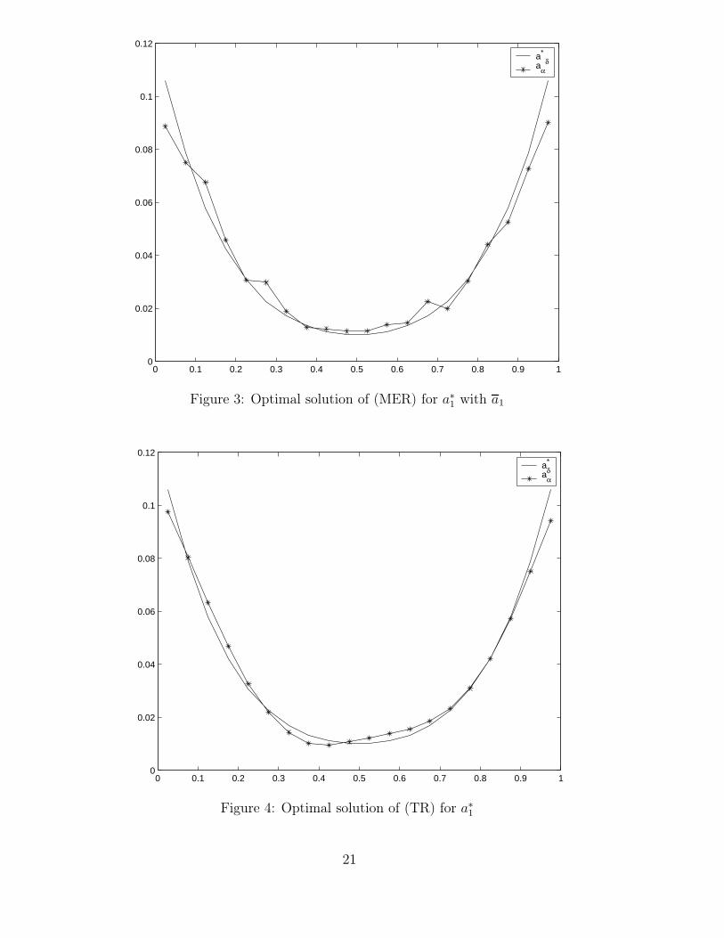
We compared for T = 1 the behavior of the maximum entropy regularization (MER)according to (20) and of the second order Tikhonov regularization (TR) according to (43)implemented in a discretized form for the convex and rather smooth volatility function

a∗1(τ) = ((τ − 0.5)2 + 0.1)2 (0 ≤ τ ≤ 1)

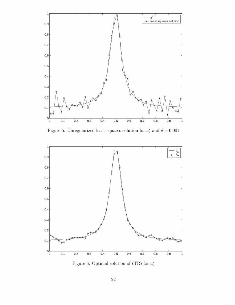
in a first study and for the volatility function

a∗2(τ) = 0.1 +

0.9

1 + 100(2τ − 1)2(0 ≤ τ ≤ 1)

with a sharp peak at the point τ = 0.5 in a second study.

For our case studies we approximated the functions a by the vector a = (a1, . . . , aN)T

with ai = a(

2i−12N

). Using the values X = 0.6, K = 0.5, r = 0.05 we computed the exact

option price data u∗j = u∗(tj) at time tj := j

N(j = 1, . . . , N) according to formula (7).

Perturbed by a random noise vector η = (η1, . . . , ηN)T ∈ IRN with normally distributedcomponents ηi ∼ N (0, 1), which are i.i.d. for i = 1, 2, ..., n, the vector u∗ := (u∗

1, . . . , u∗N)T

gives the noisy data vector uδ with components

uδj := u∗

j + δ‖u∗‖2

‖η‖2

ηj (j = 1, . . . , N),

15

where ‖ · ‖2 denotes the Euclidean vector norm. The discrete regularized solutionsaδ

α =((aδ

α)1, . . . , (aδα)N

)T were determined as minimizers of discrete analogs of the ex-tremal problems (23) and (43) and the accuracy of approximate solutions was measured

in the Manhattan norm ‖aδα−a∗‖1 =

N∑j=1

|(aδα)j −a∗

j |, which is proportional to the discrete

L1-norm.

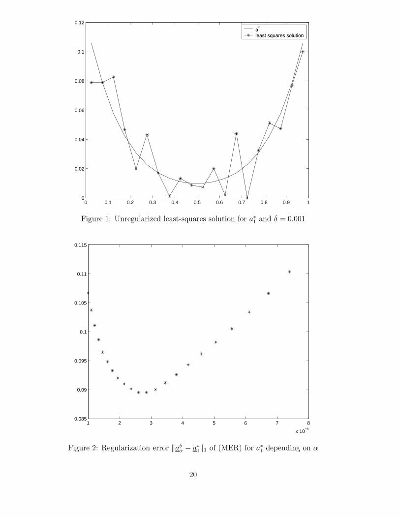
In the first case study with exact solution a∗1 we used the discretization level

N = 20 and in both studies and all figures the noise level δ = 0.001. Figure 1 showsthe unregularized solution (α = 0). Small data errors cause significant perturbationsin the least-squares solution. Therefore a regularization seems to be necessary. For themaximum entropy regularization (MER) with reference function

a1(τ) := (0.5 · (τ − 0.5)2 + 0.16)2 (0 ≤ τ ≤ 1)

the error ‖aδα − a∗

1‖1 as a function of the regularization parameter α > 0 is sketched infigure 2. Figure 3 shows for the same reference function the best solution obtained bymaximum entropy regularization minimizing the discrete L1-error norm over all regular-ization parameters α > 0. Figure 4 displays alternatively the best regularized solutioncomputed by second order Tikhonov regularization (TR).

Regularization method Error ‖aδαopt

− a∗1‖1

(TR) 0.0560(MER) with a1 0.0896(MER) with a2 0.1196

Table 1: Accuracy of best regularized solutions for smooth solution

Table 1 compares the errors ‖aδα − a∗

1‖1 for the best regularized solutions aδα obtained

by (TR) and by (MER) with the two different reference functions a1 as defined above and

a2(τ) := 0.07 (0 ≤ τ ≤ 1).

It can be concluded, that for the smooth function a∗1 to be recovered the best solutions were

obtained by Tikhonov regularization of second order. Hence, for the test function a∗1 the

smoothness information, which is used by Tikhonov regularization of second order, seemsto be more appropriate than the information about the shape of a∗, which is reflected bythe reference function a1 in the context of maximum entropy regularization. In absenceof any information about the shape of a∗ one has to use a constant reference function, forexample a2, which does not provide acceptable regularized solutions here.

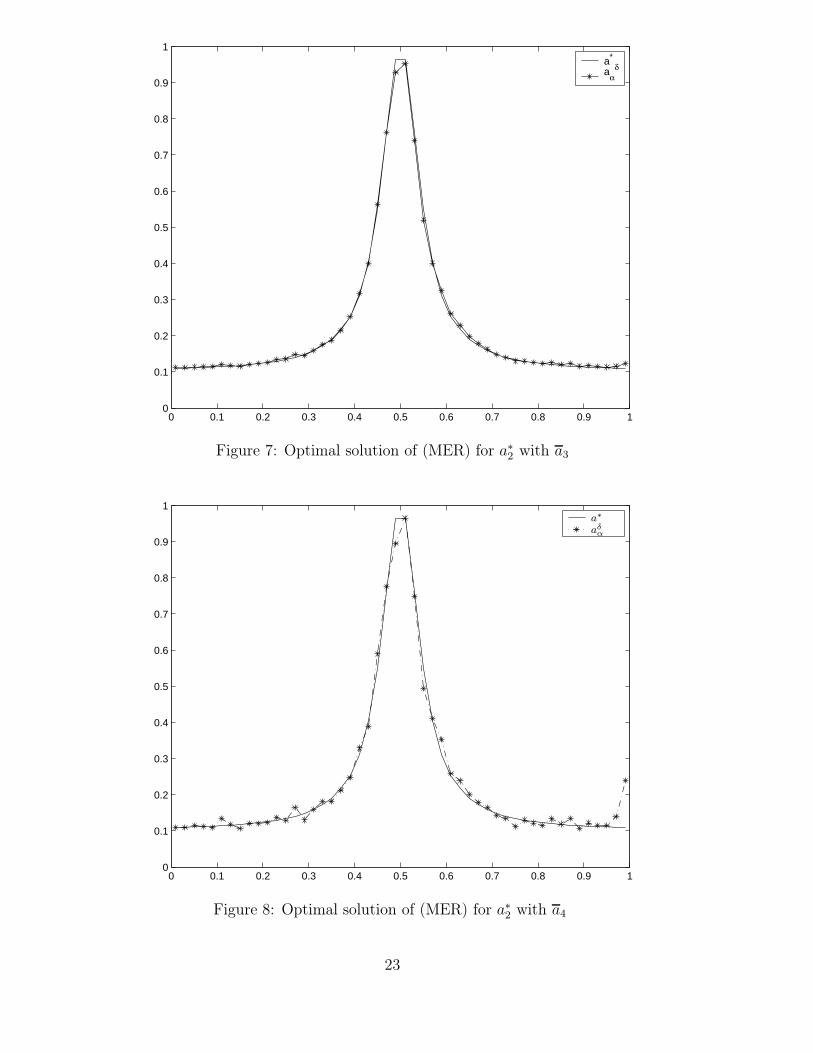
In our second case study with exact solution a∗2 we used N = 50 and compared (TR)

and (MER) with the well-approximating reference function

a3(τ) = 0.12 + 0.5/(1 + 100(2τ − 1)2) (0 ≤ τ ≤ 1)

and with the constant reference function

a4(τ) := 0.5 (0 ≤ τ ≤ 1).

16

The figures 5, 6, 7, 8 show the unregularized solution, the best regularized solution ob-tained by (TR) and by (MER) with reference function a3 and a4, respectively. The bestpossible errors ‖aδ

α − a∗2‖1 are compared in table 2. Here the maximum entropy results

with the reference function a3 are better than the results obtained with (TR). On theother hand, (MER) with reference function a4 leads to a regularized solution, which ap-proximates the exact solution a∗

2 quite well for 0 < τ < 0.95, but deviates at the rightend of the interval, because for τ ≈ 1 the data information decreases (cf. formulae (6),(7) and (36)) and the influence of the reference function dominates.

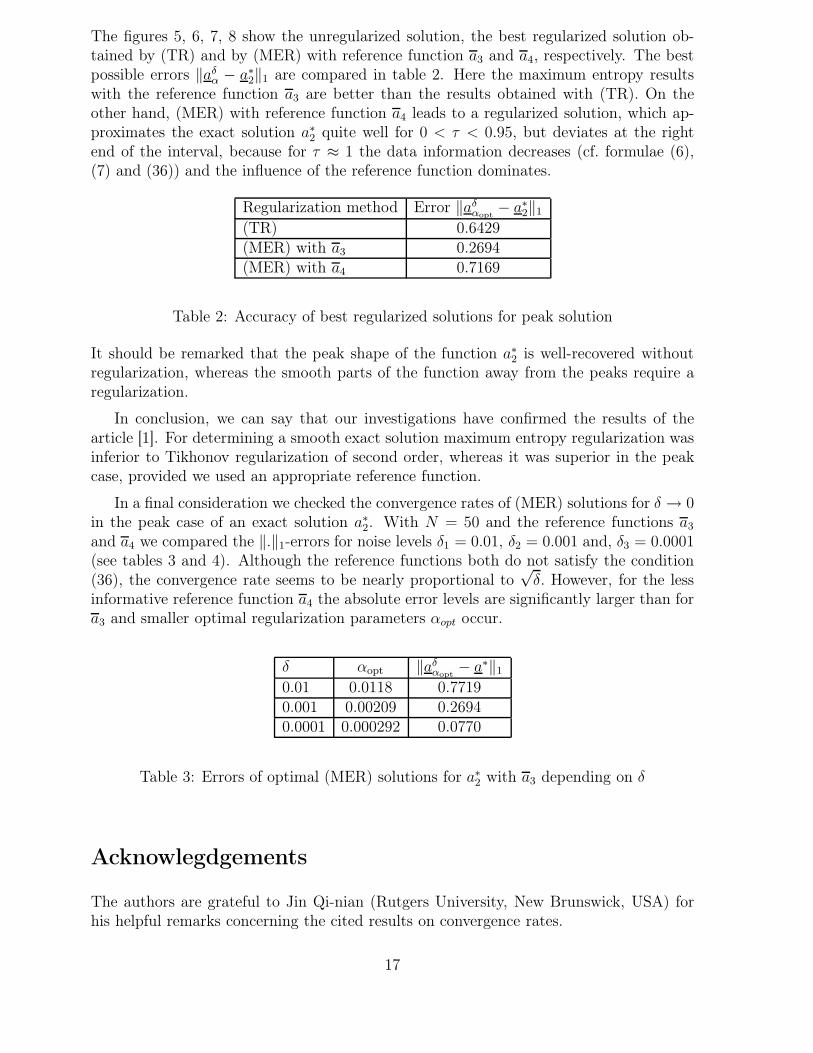
Regularization method Error ‖aδαopt

− a∗2‖1

(TR) 0.6429(MER) with a3 0.2694(MER) with a4 0.7169

Table 2: Accuracy of best regularized solutions for peak solution

It should be remarked that the peak shape of the function a∗2 is well-recovered without

regularization, whereas the smooth parts of the function away from the peaks require aregularization.

In conclusion, we can say that our investigations have confirmed the results of thearticle [1]. For determining a smooth exact solution maximum entropy regularization wasinferior to Tikhonov regularization of second order, whereas it was superior in the peakcase, provided we used an appropriate reference function.

In a final consideration we checked the convergence rates of (MER) solutions for δ → 0in the peak case of an exact solution a∗

2. With N = 50 and the reference functions a3

and a4 we compared the ‖.‖1-errors for noise levels δ1 = 0.01, δ2 = 0.001 and, δ3 = 0.0001(see tables 3 and 4). Although the reference functions both do not satisfy the condition(36), the convergence rate seems to be nearly proportional to

√δ. However, for the less

informative reference function a4 the absolute error levels are significantly larger than fora3 and smaller optimal regularization parameters αopt occur.

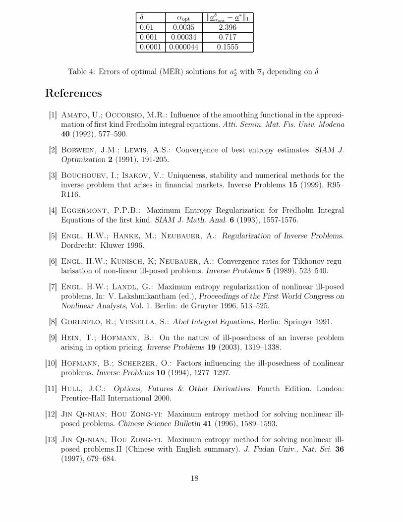
δ αopt ‖aδαopt

− a∗‖1

0.01 0.0118 0.77190.001 0.00209 0.26940.0001 0.000292 0.0770

Table 3: Errors of optimal (MER) solutions for a∗2 with a3 depending on δ

Acknowlegdgements

The authors are grateful to Jin Qi-nian (Rutgers University, New Brunswick, USA) forhis helpful remarks concerning the cited results on convergence rates.

17

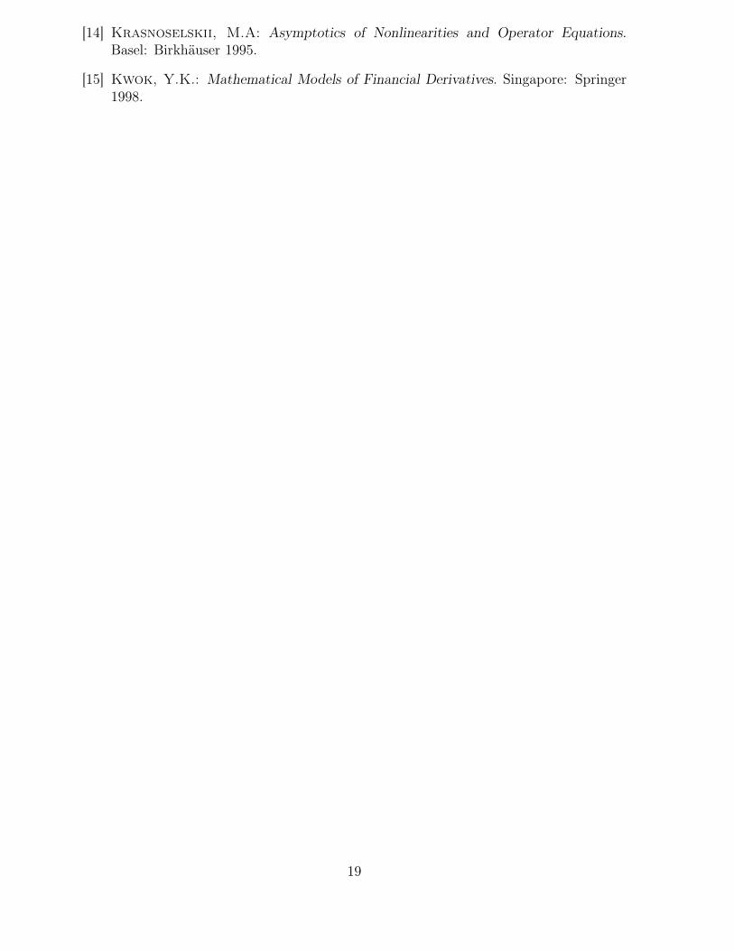
δ αopt ‖aδαopt

− a∗‖1

0.01 0.0035 2.3960.001 0.00034 0.7170.0001 0.000044 0.1555

Table 4: Errors of optimal (MER) solutions for a∗2 with a4 depending on δ

References

[1] Amato, U.; Occorsio, M.R.: Influence of the smoothing functional in the approxi-mation of first kind Fredholm integral equations. Atti. Semin. Mat. Fis. Univ. Modena40 (1992), 577–590.

[2] Borwein, J.M.; Lewis, A.S.: Convergence of best entropy estimates. SIAM J.Optimization 2 (1991), 191-205.

[3] Bouchouev, I.; Isakov, V.: Uniqueness, stability and numerical methods for theinverse problem that arises in financial markets. Inverse Problems 15 (1999), R95–R116.

[4] Eggermont, P.P.B.: Maximum Entropy Regularization for Fredholm IntegralEquations of the first kind. SIAM J. Math. Anal. 6 (1993), 1557-1576.

[5] Engl, H.W.; Hanke, M.; Neubauer, A.: Regularization of Inverse Problems.Dordrecht: Kluwer 1996.

[6] Engl, H.W.; Kunisch, K; Neubauer, A.: Convergence rates for Tikhonov regu-larisation of non-linear ill-posed problems. Inverse Problems 5 (1989), 523–540.

[7] Engl, H.W.; Landl, G.: Maximum entropy regularization of nonlinear ill-posedproblems. In: V. Lakshmikantham (ed.), Proceedings of the First World Congress onNonlinear Analysts, Vol. 1. Berlin: de Gruyter 1996, 513–525.

[8] Gorenflo, R.; Vessella, S.: Abel Integral Equations. Berlin: Springer 1991.

[9] Hein, T.; Hofmann, B.: On the nature of ill-posedness of an inverse problemarising in option pricing. Inverse Problems 19 (2003), 1319–1338.

[10] Hofmann, B.; Scherzer, O.: Factors influencing the ill-posedness of nonlinearproblems. Inverse Problems 10 (1994), 1277–1297.

[11] Hull, J.C.: Options, Futures & Other Derivatives. Fourth Edition. London:Prentice-Hall International 2000.

[12] Jin Qi-nian; Hou Zong-yi: Maximum entropy method for solving nonlinear ill-posed problems. Chinese Science Bulletin 41 (1996), 1589–1593.

[13] Jin Qi-nian; Hou Zong-yi: Maximum entropy method for solving nonlinear ill-posed problems.II (Chinese with English summary). J. Fudan Univ., Nat. Sci. 36(1997), 679–684.

18

[14] Krasnoselskii, M.A: Asymptotics of Nonlinearities and Operator Equations.Basel: Birkhäuser 1995.

[15] Kwok, Y.K.: Mathematical Models of Financial Derivatives. Singapore: Springer1998.

19

0 0.1 0.2 0.3 0.4 0.5 0.6 0.7 0.8 0.9 10

0.02

0.04

0.06

0.08

0.1

0.12a*

least squares solution

Figure 1: Unregularized least-squares solution for a∗1 and δ = 0.001

1 2 3 4 5 6 7 8

x 10−4

0.085

0.09

0.095

0.1

0.105

0.11

0.115

Figure 2: Regularization error ‖aδα − a∗

1‖1 of (MER) for a∗1 depending on α

20

0 0.1 0.2 0.3 0.4 0.5 0.6 0.7 0.8 0.9 10

0.02

0.04

0.06

0.08

0.1

0.12a*

aαδ

Figure 3: Optimal solution of (MER) for a∗1 with a1

0 0.1 0.2 0.3 0.4 0.5 0.6 0.7 0.8 0.9 10

0.02

0.04

0.06

0.08

0.1

0.12a*

aαδ

Figure 4: Optimal solution of (TR) for a∗1

21

0 0.1 0.2 0.3 0.4 0.5 0.6 0.7 0.8 0.9 10

0.1

0.2

0.3

0.4

0.5

0.6

0.7

0.8

0.9

1a*

least squares solution

Figure 5: Unregularized least-squares solution for a∗2 and δ = 0.001

0 0.1 0.2 0.3 0.4 0.5 0.6 0.7 0.8 0.9 10

0.1

0.2

0.3

0.4

0.5

0.6

0.7

0.8

0.9

1a*

aαδ

Figure 6: Optimal solution of (TR) for a∗2

22

0 0.1 0.2 0.3 0.4 0.5 0.6 0.7 0.8 0.9 10

0.1

0.2

0.3

0.4

0.5

0.6

0.7

0.8

0.9

1a*

aαδ

Figure 7: Optimal solution of (MER) for a∗2 with a3

0 0.1 0.2 0.3 0.4 0.5 0.6 0.7 0.8 0.9 10

0.1

0.2

0.3

0.4

0.5

0.6

0.7

0.8

0.9

1a∗aδ

α

Figure 8: Optimal solution of (MER) for a∗2 with a4

23