on dynamical pricing model

Nonlinear Analysis:Real World Applications 3 (2002) 131–137www.elsevier.com/locate/na

On dynamical pricing model

Timur Khusainova ;∗, Boris KalitinbaFaculty of Cybernetics, Kiev University, Vladimirskaya Str., 64, Kiev 252033, Ukraine

bFaculty of Applied Mathematics, Belarus University, Fransysk Skorina Str., 4, Minsk 220050, Belarus

Received 11 June 1999; accepted 26 November 2000

Keywords: Di.erential equations; Lyapunov functions; Stability modelling

1. Introduction

In this article, the researches on dynamics of pricing proposed in [6,7] are continued.The model was constructed under the following assumptions.

1. Market has an equilibrium, i.e. there exists such 9xed vector of prices (stationarypoint), such that the desires of all customers and sellers coincide.

2. The process of price establishment is operated by “forces” of pricing participants.They are:Vi(·) desire of ith seller to increase the price of its good;Cij(·) in<uence of jth competitor on the price of ith good;Di(·) in<uence of customers of ith good;Gi(·) in<uence on price of ith good on the part of external structures;

(i; j = 1; : : : ; n).3. We assume that there is a rule of forces independence for every good and that theresult of pricing dynamics depends on the sum of composing forces.

4. The process of price variation is de9ned by the following assumptions. Speed ofprice variation is equal to weighted sum of operating forces. This is the majorassumption for modeling the dynamic processes with the help of di.erentialequations.

∗ Corresponding author.E-mail addresses: [email protected] (T. Khusainov), [email protected] (B. Kalitin).

1468-1218/01/$ - see front matter c© 2001 Elsevier Science Ltd. All rights reserved.PII: S1468 -1218(01)00018 -9

132 T. Khusainov, B. Kalitin /Nonlinear Analysis:Real World Applications 3 (2002) 131–137

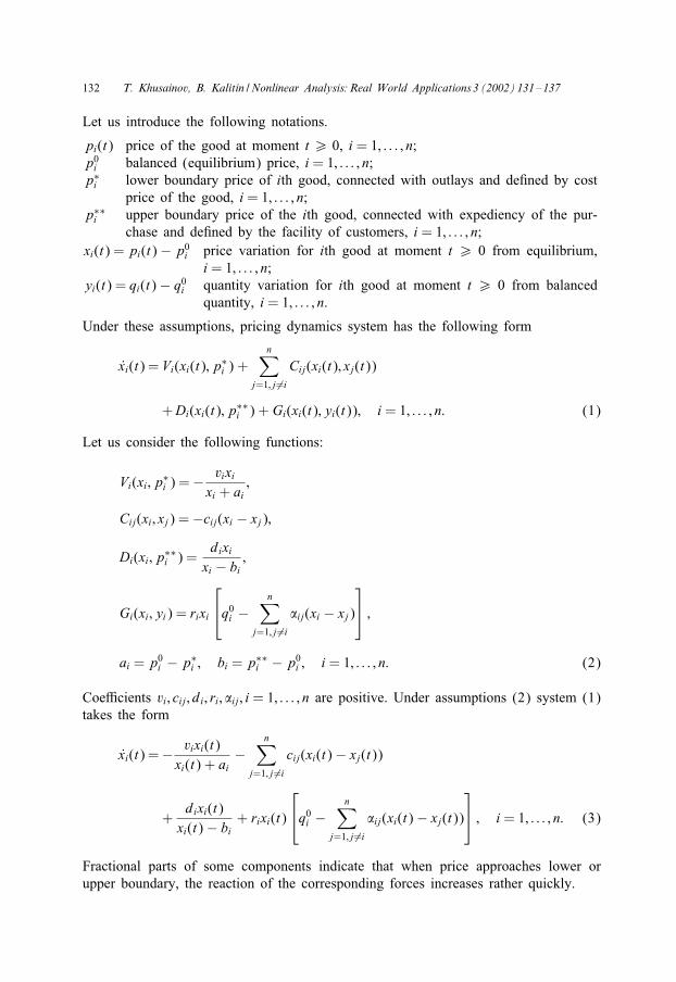
Let us introduce the following notations.

pi(t) price of the good at moment t ¿ 0, i = 1; : : : ; n;p0i balanced (equilibrium) price, i = 1; : : : ; n;p∗i lower boundary price of ith good, connected with outlays and de9ned by cost

price of the good, i = 1; : : : ; n;p∗∗i upper boundary price of the ith good, connected with expediency of the pur-

chase and de9ned by the facility of customers, i = 1; : : : ; n;xi(t) = pi(t)− p0i price variation for ith good at moment t ¿ 0 from equilibrium,

i = 1; : : : ; n;yi(t) = qi(t)− q0i quantity variation for ith good at moment t ¿ 0 from balanced

quantity, i = 1; : : : ; n.

Under these assumptions, pricing dynamics system has the following form

xi(t) = Vi(xi(t); p∗i ) +

n∑j=1; j �=i

Cij(xi(t); xj(t))

+Di(xi(t); p∗∗i ) + Gi(xi(t); yi(t)); i = 1; : : : ; n: (1)

Let us consider the following functions:

Vi(xi; p∗i ) =− vixi

xi + ai;

Cij(xi; xj) =−cij(xi − xj);

Di(xi; p∗∗i ) =

dixixi − bi

;

Gi(xi; yi) = rixi

q0i − n∑

j=1; j �=i�ij(xi − xj)

;

ai = p0i − p∗i ; bi = p∗∗

i − p0i ; i = 1; : : : ; n: (2)

CoeJcients vi; cij; di; ri; �ij; i = 1; : : : ; n are positive. Under assumptions (2) system (1)takes the form

xi(t) =− vixi(t)xi(t) + ai

−n∑

j=1; j �=icij(xi(t)− xj(t))

+dixi(t)xi(t)− bi

+ rixi(t)

q0i − n∑

j=1; j �=i�ij(xi(t)− xj(t))

; i = 1; : : : ; n: (3)

Fractional parts of some components indicate that when price approaches lower orupper boundary, the reaction of the corresponding forces increases rather quickly.

T. Khusainov, B. Kalitin /Nonlinear Analysis:Real World Applications 3 (2002) 131–137 133

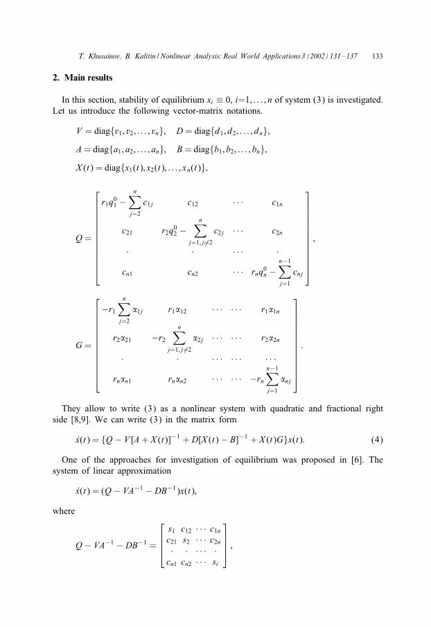
2. Main results

In this section, stability of equilibrium xi ≡ 0, i=1; : : : ; n of system (3) is investigated.Let us introduce the following vector-matrix notations.

V = diag{v1; v2; : : : ; vn}; D = diag{d1; d2; : : : ; dn};A= diag{a1; a2; : : : ; an}; B= diag{b1; b2; : : : ; bn};X (t) = diag{x1(t); x2(t); : : : ; xn(t)};

Q =

r1q01 −n∑j=2

c1j c12 · · · c1n

c21 r2q02 −n∑

j=1; j �=2c2j · · · c2n

· · · · · ·

cn1 cn2 · · · rnq0n −n−1∑j=1

cnj

;

G =

−r1n∑j=2

�1j r1�12 · · · · · · r1�1n

r2�21 −r2n∑

j=1; j �=2�2j · · · · · · r2�2n

· · · · · · · · · · ·

rn�n1 rn�n2 · · · · · · −rnn−1∑j=1

�nj

:

They allow to write (3) as a nonlinear system with quadratic and fractional rightside [8,9]. We can write (3) in the matrix form

x(t) = {Q − V [A+ X (t)]−1 + D[X (t)− B]−1 + X (t)G}x(t): (4)

One of the approaches for investigation of equilibrium was proposed in [6]. Thesystem of linear approximation

x(t) = (Q − VA−1 − DB−1)x(t);

where

Q − VA−1 − DB−1 =

s1 c12 · · · c1nc21 s2 · · · c2n· · · · · ·cn1 cn2 · · · si

;


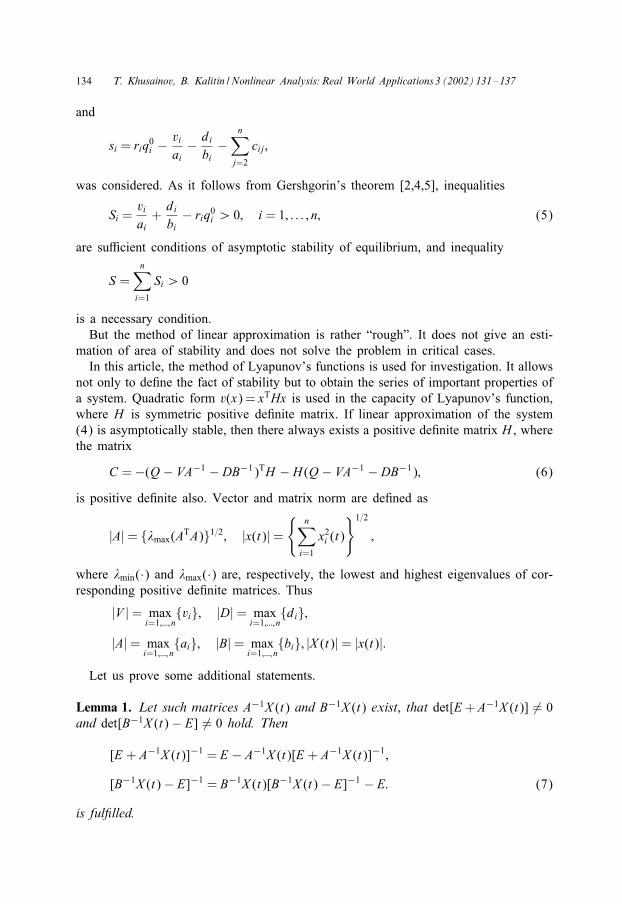
and

si = riq0i −viai

− dibi

−n∑j=2

cij;

was considered. As it follows from Gershgorin’s theorem [2,4,5], inequalities

Si =viai+dibi

− riq0i ¿ 0; i = 1; : : : ; n; (5)

are suJcient conditions of asymptotic stability of equilibrium, and inequality

S =n∑i=1

Si ¿ 0

is a necessary condition.But the method of linear approximation is rather “rough”. It does not give an esti-

mation of area of stability and does not solve the problem in critical cases.In this article, the method of Lyapunov’s functions is used for investigation. It allows

not only to de9ne the fact of stability but to obtain the series of important properties ofa system. Quadratic form v(x) = xTHx is used in the capacity of Lyapunov’s function,where H is symmetric positive de9nite matrix. If linear approximation of the system(4) is asymptotically stable, then there always exists a positive de9nite matrix H , wherethe matrix

C =−(Q − VA−1 − DB−1)TH − H (Q − VA−1 − DB−1); (6)

is positive de9nite also. Vector and matrix norm are de9ned as

|A|= {�max(ATA)}1=2; |x(t)|={

n∑i=1

x2i (t)

}1=2

;

where �min(·) and �max(·) are, respectively, the lowest and highest eigenvalues of cor-responding positive de9nite matrices. Thus

|V |= maxi=1;:::; n

{vi}; |D|= maxi=1;:::; n

{di};

|A|= maxi=1;:::; n

{ai}; |B|= maxi=1;:::; n

{bi}; |X (t)|= |x(t)|:

Let us prove some additional statements.

Lemma 1. Let such matrices A−1X (t) and B−1X (t) exist, that det[E+A−1X (t)] �= 0and det[B−1X (t)− E] �= 0 hold. Then

[E + A−1X (t)]−1 = E − A−1X (t)[E + A−1X (t)]−1;

[B−1X (t)− E]−1 = B−1X (t)[B−1X (t)− E]−1 − E: (7)

is ful6lled.


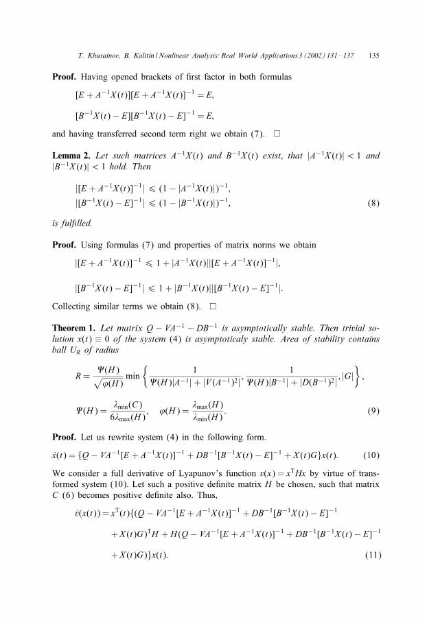
Proof. Having opened brackets of 9rst factor in both formulas

[E + A−1X (t)][E + A−1X (t)]−1 = E;

[B−1X (t)− E][B−1X (t)− E]−1 = E;

and having transferred second term right we obtain (7).

Lemma 2. Let such matrices A−1X (t) and B−1X (t) exist; that |A−1X (t)|¡ 1 and|B−1X (t)|¡ 1 hold. Then

|[E + A−1X (t)]−1|6 (1− |A−1X (t)|)−1;|[B−1X (t)− E]−1|6 (1− |B−1X (t)|)−1; (8)

is ful6lled.

Proof. Using formulas (7) and properties of matrix norms we obtain

|[E + A−1X (t)]−1 6 1 + |A−1X (t)||[E + A−1X (t)]−1|;

|[B−1X (t)− E]−1|6 1 + |B−1X (t)||[B−1X (t)− E]−1|:Collecting similar terms we obtain (8).

Theorem 1. Let matrix Q − VA−1 − DB−1 is asymptotically stable. Then trivial so-lution x(t) ≡ 0 of the system (4) is asymptoticaly stable. Area of stability containsball UR of radius

R=$(H)√’(H)

min{

1$(H)|A−1|+ |V (A−1)2| ;

1$(H)|B−1|+ |D(B−1)2| ; |G|

};

$(H) =�min(C)6�max(H)

; ’(H) =�max(H)�min(H)

: (9)

Proof. Let us rewrite system (4) in the following form.

x(t) = {Q − VA−1[E + A−1X (t)]−1 + DB−1[B−1X (t)− E]−1 + X (t)G}x(t): (10)

We consider a full derivative of Lyapunov’s function v(x) = xTHx by virtue of trans-formed system (10). Let such a positive de9nite matrix H be chosen, such that matrixC (6) becomes positive de9nite also. Thus,

v(x(t)) = xT(t){(Q − VA−1[E + A−1X (t)]−1 + DB−1[B−1X (t)− E]−1

+X (t)G)TH + H (Q − VA−1[E + A−1X (t)]−1 + DB−1[B−1X (t)− E]−1

+X (t)G)}x(t): (11)


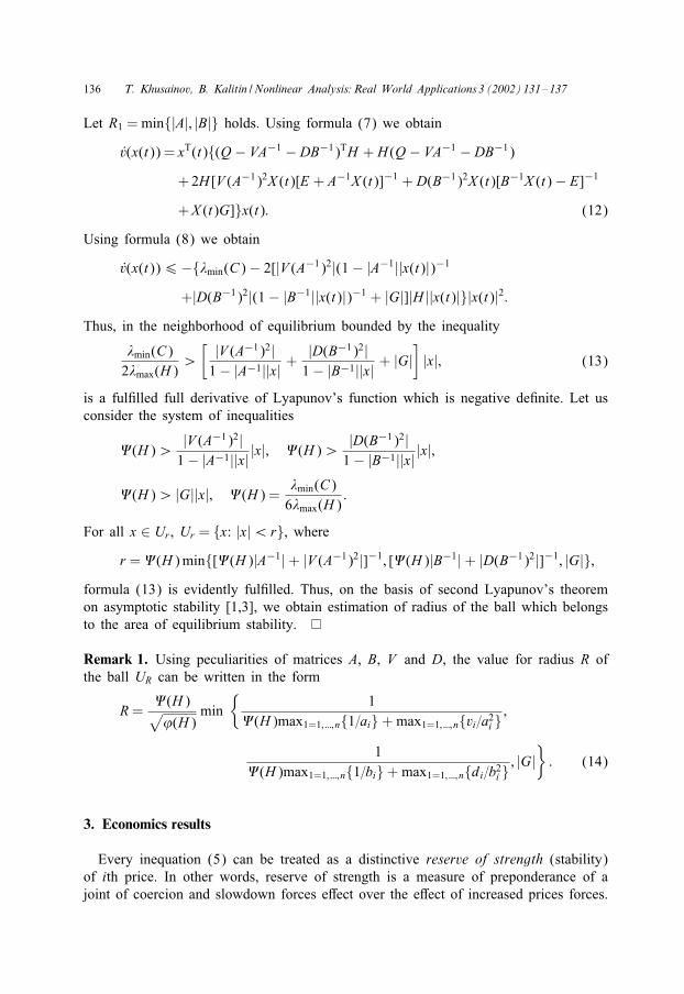
Let R1 = min{|A|; |B|} holds. Using formula (7) we obtainv(x(t)) = xT(t){(Q − VA−1 − DB−1)TH + H (Q − VA−1 − DB−1)

+2H [V (A−1)2X (t)[E + A−1X (t)]−1 + D(B−1)2X (t)[B−1X (t)− E]−1

+X (t)G]}x(t): (12)

Using formula (8) we obtain

v(x(t))6−{�min(C)− 2[|V (A−1)2|(1− |A−1||x(t)|)−1

+|D(B−1)2|(1− |B−1||x(t)|)−1 + |G|]|H ||x(t)|}|x(t)|2:Thus, in the neighborhood of equilibrium bounded by the inequality

�min(C)2�max(H)

¿[ |V (A−1)2|1− |A−1||x| +

|D(B−1)2|1− |B−1||x| + |G|

]|x|; (13)

is a ful9lled full derivative of Lyapunov’s function which is negative de9nite. Let usconsider the system of inequalities

$(H)¿|V (A−1)2|1− |A−1||x| |x|; $(H)¿

|D(B−1)2|1− |B−1||x| |x|;

$(H)¿ |G||x|; $(H) =�min(C)6�max(H)

:

For all x ∈ Ur , Ur = {x: |x|¡r}, wherer =$(H)min{[$(H)|A−1|+ |V (A−1)2|]−1; [$(H)|B−1|+ |D(B−1)2|]−1; |G|};

formula (13) is evidently ful9lled. Thus, on the basis of second Lyapunov’s theoremon asymptotic stability [1,3], we obtain estimation of radius of the ball which belongsto the area of equilibrium stability.

Remark 1. Using peculiarities of matrices A, B, V and D, the value for radius R ofthe ball UR can be written in the form

R=$(H)√’(H)

min{

1$(H)max1=1; :::; n{1=ai}+max1=1; :::; n{vi=a2i }

;

1$(H)max1=1; :::; n{1=bi}+max1=1; :::; n{di=b2i }

; |G|}: (14)

3. Economics results

Every inequation (5) can be treated as a distinctive reserve of strength (stability)of ith price. In other words, reserve of strength is a measure of preponderance of ajoint of coercion and slowdown forces e.ect over the e.ect of increased prices forces.


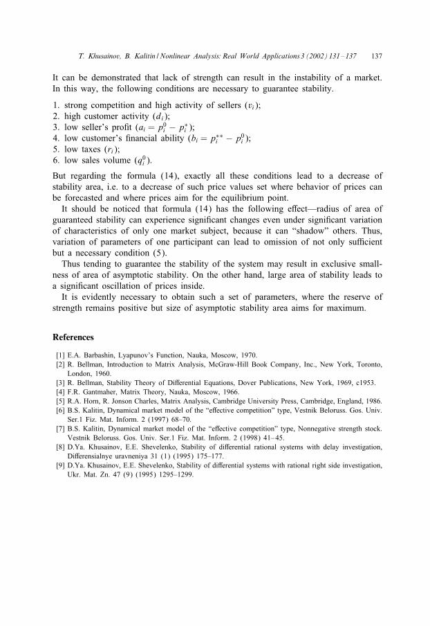
It can be demonstrated that lack of strength can result in the instability of a market.In this way, the following conditions are necessary to guarantee stability.

1. strong competition and high activity of sellers (vi);2. high customer activity (di);3. low seller’s pro9t (ai = p0i − p∗

i );4. low customer’s 9nancial ability (bi = p∗∗

i − p0i );5. low taxes (ri);6. low sales volume (q0i ).

But regarding the formula (14), exactly all these conditions lead to a decrease ofstability area, i.e. to a decrease of such price values set where behavior of prices canbe forecasted and where prices aim for the equilibrium point.It should be noticed that formula (14) has the following e.ect—radius of area of

guaranteed stability can experience signi9cant changes even under signi9cant variationof characteristics of only one market subject, because it can “shadow” others. Thus,variation of parameters of one participant can lead to omission of not only suJcientbut a necessary condition (5).Thus tending to guarantee the stability of the system may result in exclusive small-

ness of area of asymptotic stability. On the other hand, large area of stability leads toa signi9cant oscillation of prices inside.It is evidently necessary to obtain such a set of parameters, where the reserve of

strength remains positive but size of asymptotic stability area aims for maximum.

References

[1] E.A. Barbashin, Lyapunov’s Function, Nauka, Moscow, 1970.[2] R. Bellman, Introduction to Matrix Analysis, McGraw-Hill Book Company, Inc., New York, Toronto,

London, 1960.[3] R. Bellman, Stability Theory of Di.erential Equations, Dover Publications, New York, 1969, c1953.[4] F.R. Gantmaher, Matrix Theory, Nauka, Moscow, 1966.[5] R.A. Horn, R. Jonson Charles, Matrix Analysis, Cambridge University Press, Cambridge, England, 1986.[6] B.S. Kalitin, Dynamical market model of the “e.ective competition” type, Vestnik Beloruss. Gos. Univ.

Ser.1 Fiz. Mat. Inform. 2 (1997) 68–70.[7] B.S. Kalitin, Dynamical market model of the “e.ective competition” type, Nonnegative strength stock.

Vestnik Beloruss. Gos. Univ. Ser.1 Fiz. Mat. Inform. 2 (1998) 41–45.[8] D.Ya. Khusainov, E.E. Shevelenko, Stability of di.erential rational systems with delay investigation,

Di.erensialnye uravneniya 31 (1) (1995) 175–177.[9] D.Ya. Khusainov, E.E. Shevelenko, Stability of di.erential systems with rational right side investigation,

Ukr. Mat. Zn. 47 (9) (1995) 1295–1299.

on dynamical pricing model

Documents