on discriminative bayesian network classifiers and logistic

Machine Learning, 59, 267–296, 20052005 Springer Science + Business Media, Inc. Manufactured in The Netherlands.

On Discriminative Bayesian Network Classifiersand Logistic RegressionTEEMU ROOS [email protected]

HANNES WETTIGComplex Systems Computation Group, Helsinki Institute for Information Technology, P.O. Box 9800,FI-02015 TKK, Finland

PETER GRUNWALDCentrum voor Wiskunde en Informatica, P.O. Box 94079, NL-1090 GB Amsterdam, The Netherlands

PETRI MYLLYMAKI

HENRY TIRRIComplex Systems Computation Group, Helsinki Institute for Information Technology, P.O. Box 9800,FI-02015 TKK, Finland

Editors: Pedro Larranaga, Jose A. Lozano, Jose M. Pena and Inaki Inza

Abstract. Discriminative learning of the parameters in the naive Bayes model is known to be equivalent toa logistic regression problem. Here we show that the same fact holds for much more general Bayesian networkmodels, as long as the corresponding network structure satisfies a certain graph-theoretic property. The propertyholds for naive Bayes but also for more complex structures such as tree-augmented naive Bayes (TAN) as wellas for mixed diagnostic-discriminative structures. Our results imply that for networks satisfying our property,the conditional likelihood cannot have local maxima so that the global maximum can be found by simple localoptimization methods. We also show that if this property does not hold, then in general the conditional likelihoodcan have local, non-global maxima. We illustrate our theoretical results by empirical experiments with localoptimization in a conditional naive Bayes model. Furthermore, we provide a heuristic strategy for pruning thenumber of parameters and relevant features in such models. For many data sets, we obtain good results withheavily pruned submodels containing many fewer parameters than the original naive Bayes model.

Keywords: Bayesian classifiers, Bayesian networks, discriminative learning, logistic regression

1. Introduction

Bayesian network models are widely used for discriminative prediction tasks such asclassification. The parameters of such models are often determined using ‘unsupervised’methods such as maximization of the joint likelihood (Friedman, Geiger, & Goldszmidt,1997). In recent years, it has been recognized, both theoretically and experimentally, that inmany situations it is better to use a matching ‘discriminative’ or ‘supervised’ learning algo-rithm such as conditional likelihood maximization (Friedman, Geiger, & Goldszmidt, 1997;Greiner, Grove, & Schuurmans, 1997; Ng & Jordan, 2001; Kontkanen, Myllymaki, & Tirri,2001). In this paper, we show that if the network structure satisfies a certain simple graph-theoretic condition, then the corresponding conditional likelihood maximization problemis equivalent to logistic regression based on certain statistics of the data—different network

268 T. ROOS ET AL.

structures leading to different statistics. We thereby establish a connection between the rel-atively new methods of Bayesian network classifier learning and the established statisticalmethod of logistic regression, which has a long history and which has been thoroughlystudied in the past (McLachlan, 1992). One of the main implications of this connection isthe following: if the condition mentioned above holds for the network structure, the corre-sponding conditional likelihood of the Bayesian network model cannot have local optimaso that the global optimum can be found by local optimization methods. Other implications,as well as our additional results are summarized below.

Section 2 reviews Bayesian network models, Bayesian network classifiers and discrim-inative learning of Bayesian network models, based on the conditional rather than jointlikelihood. Consider a network structure (directed acyclic graph, DAG) B on a tuple ofdiscrete-valued random variables (X0, . . . , XM). In Section 2.4 we define our main concept,the conditional Bayesian network model MB. This is the set of conditional distributions ofclass variable X0 given the feature variables X1, . . . , XM , induced by the Bayesian networkmodel based on structure B that can be achieved with non-zero parameters. We define foreach network structure B a corresponding canonical form B∗ that facilitates comparisonwith logistic regression. Graph B∗ is simply the Markov blanket of the class variable X0

in B, with arcs added to make all parents of X0 fully connected. We show that the modelsMB and MB∗

are identical: even though the set of joint distributions on (X0, . . . , XM)corresponding to B and B∗ may not coincide, the set of conditional distributions of X0

given (X1, . . . , XM) is the same for both graphs.Section 3 reviews the multiple logistic regression model. We provide a reparameteri-

zation of conditional Bayesian network models MB such that the parameters in the newparameterization correspond to logarithms of parameters in the standard Bayesian networkparameterization. In this way, each conditional Bayesian network model is mapped to alogistic regression model. However, in some cases the parameters of this logistic regres-sion model are not allowed to vary freely. In other words, the Bayesian network modelcorresponds to a subset of a logistic regression model rather than a ‘full’ logistic regressionmodel. This is established in our Theorem 2.

In Section 4 we present our main result (Theorem 3) which provides a general conditionon the network structure B under which the Bayesian network model is mapped to a fulllogistic regression model with freely varying parameters. This condition is very simple: itrequires the corresponding canonical structure B∗ to be a perfect DAG, meaning that allnodes are moral nodes. It is satisfied by, for example, the naive Bayes model, the tree-augmented naive Bayes model (TAN), but also for more complicated models in which theclass node has parents.

The conditional log-likelihood for logistic regression models is a concave function of theparameters. Therefore, in the new parameterization the conditional log-likelihood becomesa concave function of the parameters that under the perfectness condition are allowed tovary freely over the convex set R

k . This implies that we can find the global maximumin the conditional likelihood surface by simple local optimization techniques such as hill-climbing. This result still leaves open the possibility that there are no network structures forwhich the conditional likelihood surface has local, non-global maxima. This would makeperfectness a superfluous condition. Our second result (Theorem 4) shows that this is not

BAYESIAN NETWORK CLASSIFIERS AND LOGISTIC REGRESSION 269

the case: there are very simple network structures B whose canonical version B∗ is notperfect, and for which the conditional likelihood can exhibit local, non-global maxima.

Section 5 discusses the various issues arising when implementing local optimizationmethods for finding the maximum conditional likelihood of Bayesian network modelswhose structure B satisfies the perfectness property. These involve choosing the appropriateparameterization, dealing with model selection (parameter/feature pruning), missing dataand flat regions of the conditional likelihood surface, which we handle by introducingBayesian parameter priors. It turns out that in the standard parameterization of a Bayesiannetwork, the conditional likelihood may be non-concave, even if the Bayesian networkcorresponds to a logistic regression model. Therefore, optimization should be performedin the logistic parameterization in which the likelihood is concave. Finally, we introducethe algorithms of our experiments here, including a heuristic algorithm for pruning theconditional naive Bayes model.

Section 6 reports the results of these experiments. One of our main findings is that ourpruning strategy leads to considerably simpler models that are competitive against bothnaive Bayes and conditional naive Bayes with the full set of features in terms of predictiveperformance.

Viewing Bayesian network models as subsets of logistic regression models has beensuggested earlier in papers such as Heckerman and Meek (1997a), Ng and Jordan (2001),and Greiner and Zhou (2002). Also, the concavity of the log-likelihood surface for logisticregression is a well-known result. Our main contribution is to supply the condition underwhich Bayesian network models correspond to logistic regression with completely freelyvarying parameters. Only then can we guarantee that there are no local maxima in thelikelihood surface. As a direct consequence of our result, we show that the conditionallikelihood of, for instance, the tree-augmented naive Bayes (TAN) model has no localnon-global maxima.

2. Bayesian network classifiers

We start with some notation and basic properties of Bayesian networks. For more informa-tion see, e.g., Pearl (1988) and Lauritzen (1996).

2.1. Preliminaries and notation

Consider a discrete random vector X = (X0, X1, . . . , XM), where each variable Xi takesvalues in {1, . . . , ni}. Let B be a directed acyclic graph (DAG) over X, that factorizes P(X)into

P(X) =M∏

i=0

P(Xi | Pai ), (1)

where Pai ⊆ {X0, . . . , XM} is the parent set of variable Xi in B. Such a model is usuallyparameterized by vectors θB with components of the form θB

xi |paidefined by

θBxi |pai

:= P(Xi = xi | Pai = pai ), (2)

270 T. ROOS ET AL.

where pai is any configuration (set of values) for the parents Pai of Xi. Whenever we wantto emphasize that each pai is determined by the complete data vector x = (x0, . . . , xM),we write pai (x) to denote the configuration of Pai in B given by the vector x. For a givendata vector x = (x0, x1 . . . , xM), we sometimes need to consider a modified vector wherex0 is replaced by x ′

0 and the other entries remain the same. We then write pai (x′0, x) for the

configuration of Pai given by (x ′0, x1, . . . , xM ).

We are interested in predicting some class variable Xl for some l∈{0, . . . , M} conditionedon all Xi, i �= l. Without loss of generality we may assume that l = 0 (i.e., X0 is the classvariable) and that the children of X0 in B are {X1, . . . , Xm} for some m ≤ M. For instance,in the so-called naive Bayes model we have m = M and the children of the class variableX0 are independent given the value of X0. The Bayesian network model corresponding toB is the set of all distributions satisfying the conditional independencies encoded in B.

Conditional distributions for the class variable given the other variables can be writtenas

P(x0 | x1, . . . , xM , θB) = P(x0, x1, . . . , xM | θB)∑n0

x ′0=1 P(x ′

0, x1, . . . , xM | θB)

= θBx0|pa0(x)

∏Mi=1 θB

xi |pai (x)∑n0

x ′0=1 θB

x ′0|pa0(x)

∏Mi=1 θB

xi |pai (x′0,x)

. (3)

2.2. Bayesian network classifiers

A Bayesian network model can be used both for probabilistic prediction and for classifica-tion. By probabilistic prediction we mean a game where given a query vector (x1, . . . , xM),we must output a conditional distribution P(X0|x1, . . . , xM) for the class variable X0. Underthe logarithmic loss function (log-loss) we incur−ln P(x0 | x1, . . . , xM) units of loss wherex0 is the actual outcome. If we successively predict class variable outcomes x1

0 , x20 , . . . , x N

0given query vectors (x1, . . . , xM)1, . . . , (x1, . . . , xM)N using the same P , then the logarithmicloss function is just minus the conditional log-likelihood of x1

0 , x20 , . . . , x N

0 given the queryvectors, a standard statistical measure. By classification we mean the scenario where givena query vector we must output a single value, x0 of X0 that we consider the most likelyoutcome. Under 0/1 loss the loss is zero if our guess was correct and one otherwise.

Given a Bayesian network model, the corresponding Bayesian network classifier(Friedman, Geiger, & Goldszmidt, 1997) uses (3) for both prediction and classification.Given a parameter vector θB, under the log-loss we output the conditional distribution givenby (3) and under the 0/1 loss we choose as our guess the class value x0 maximizing (3). Ifthe distribution indexed by the parameter vector is actually the distribution generating thedata vectors, then in both cases this is the Bayes optimal choice.

In order to predict and/or classify new instances based on some training data, we need tofix a method to infer good parameter values based on the training data. A commonly usedmethod is to maximize the likelihood, or equivalently the log-likelihood, of the trainingdata. Given a complete data-matrix D = (x1, . . . , xN ), the (full) log-likelihood, LL(D; θB),with parameters θB is given by


L L(D; θB) :=N∑

j=1

ln P(x j

0 , . . . , x jM | θB

) =N∑

j=1

M∑i=0

ln P(x j

i | pai (xj ), θB

). (4)

Taking the derivative wrt. θB shows that for complete data the maximum is achieved bysetting for each xi and pai

θBxi |pai

(D) = n[xi ,pai ]

n[pai ], (5)

where n[xi ,pai ] and n[pai ] are respectively the numbers of data vectors with Xi = xi , Pai =pai and Pai = pai . In case the data contain missing values, there is no closed form solutionbut iterative algorithms such as the Expectation-Maximization algorithm (Dempster, Laird,& Rubin, 1977; McLachlan & Krishnan, 1997), or local search methods such as gradientascent (Russell et al., 1995; Thiesson, 1995) can be applied.

In the M-closed case (Bernardo & Smith, 1994), i.e. the case in which the data generatingdistribution can be represented with the Bayesian network B, maximizing the full likelihoodis a consistent method of estimating the joint distribution of X. The joint distributionof X given the maximum likelihood (ML) parameters converges (with growing samplesize) to the generating distribution. Thus, also the conditional distributions of the classvariable given the other variables and the maximum likelihood parameters converge to thetrue conditional distribution. As a consequence, the maximum likelihood plug-in classifierobtained by plugging (5) into (3) converges to the Bayes optimal classifier. This holds forboth the 0/1 loss and the logarithmic loss.

2.3. Discriminative parameter learning

In the context of predicting the class variable given the other variables, the full log-likelihood is not the most natural objective function since it does not take into account thediscriminative or supervised nature of the prediction task. A more focused version is theconditional log-likelihood, defined as

C L L(D; θB) :=N∑

j=1

ln P(x j

0 | x j1 . . . , x j

M , θB), (6)

where P(x j0 | x j

1 . . . , x jM , θB) is given by (3). It is important to note that (3), appearing in

(6), is not one of the terms in (4) unless Pa0 = {X1, . . . , XM}, i.e., unless the class variablehas only incoming arcs. If this were the case, the θx0|pa0

maximizing the full likelihoodwould also maximize the conditional likelihood. Due to the normalization over possiblevalues of X0 in (3), the parameters maximizing conditional likelihood (6) are not given by(5). In fact no closed-form solution is known (Friedman, Geiger, & Goldszmidt, 1997).

Maximizing the conditional likelihood is a consistent method for estimating the con-ditional distributions of the class variable in the M-closed case, just like maximizing thefull likelihood. However, there is a crucial difference between the two methods in the case

272 T. ROOS ET AL.

where the generating distribution is not in the model class, i.e., some of the independenceassumptions inherent to the Bayesian network structure B are violated. In this M-open caseit is clear that no plug-in predictor can be guaranteed to converge to the Bayes optimalclassifier. However, in probabilistic prediction under log-loss, maximizing the conditionallikelihood converges to the best possible distribution in the model class, in that it minimizesthe expected conditional log loss. To see this, let Q, P be two distributions on (X0, . . . , XM)and define the conditional Kullback-Leibler divergence as

Dcond(Q‖P) := EX0,...,X M lnQ(X0 | X1, . . . , X M )

P(X0 | X1, . . . , X M ), (7)

where the expectation is taken with respect to Q. The Kullback-Leibler divergence gives theexpected additional log-loss over the best possible distribution given by Q (see Appendix Ain Friedman, Geiger, and Goldszmidt (1997)). The following proposition shows that P(· |θB

N ) converges in probability to the distribution in B minimizing expected conditionallog-loss:

Proposition 1. Let the data be i.i.d. according to any distribution Q with full support,i.e. Q(x0, x1, . . . , xM) > 0 for all vectors x with components xi ∈ {1, . . . , ni}. Then withprobability one, for all large N there exists at least one θB

N maximizing the conditionallog-likelihood (6). For any sequence of such maximizing θB

N the distribution P(· | θBN )

converges in probability to the distribution closest to Q in conditional Kullback-Leiblerdivergence.

This follows from Theorem 1 in Greiner and Zhou (2002) which gives in addition a rateof convergence in term of sample size. When maximizing the full likelihood in the M-opencase, we may not converge to the best possible distribution. In the Appendix, we give a verysimple concrete case (Example 4) such that with probability 1, the ordinary ML estimatorconverges to a parameter vector θ and the conditional ML estimator converges to anothervector θcond with

Dcond(Q ‖ P(· | θ )) = ln 2; Dcond(Q ‖ P(· | θcond)) = 1

2ln 2.

In classification the situation is not as clear cut as in log loss prediction. Nevertheless,there is both empirical and theoretical evidence that maximizing the conditional likelihoodleads to better classification as well (see Friedman, Geiger, & Goldszmidt, 1997; Ng &Jordan, 2001; Greiner & Zhou, 2002) and references therein. Theoretically, one can argueas follows. Suppose data are i.i.d. according to some distribution Q not necessarily in M.Given a distribution P(· | θB), we say θB is conditionally correct if Q(X0 | X1, . . . , XM)= P(X0 | X1, . . . , XM , θB) for all (X0, . . . , XM) that occur with positive Q-probability.Now suppose that M contains a θcond that is conditionally correct. Then θcond must alsobe the distribution that is optimal for classification; that is, the Bayes classifier based onθcond achieves the minimum expected classification error where the expectation is over thedistribution Q. As a consequence of Proposition 1, in the large N limit, the conditional


ML estimator θBN converges to θcond and hence, asymptotically, the Bayes classifier based

on the conditional ML estimator is optimal. Note that this still holds if P(· | θcond) is‘unconditionally incorrect’ in the sense that the marginal distributions Q(X1, . . . , XM) andP(X1, . . . , XM | θcond) are very different from each other.

In contrast, when maximizing the unconditional likelihood, the distribution θ that theML estimator converges to can only be guaranteed to lead to the optimal classification ruleif M contains a distribution that is fully correct, a much stronger condition. Thus, for largetraining samples, the conditional ML estimator can be shown to be optimal for classificationunder much weaker conditions than the unconditional ML estimator. This suggests (butof course does not prove) that, for large training samples, conditional ML estimators willoften achievebetter classification performance than unconditional ML estimators.

2.4. Conditional Bayesian network models

We define the conditional model MB as the set of conditional distributions that can berepresented using network B equipped with any strictly positive1parameter set θB > 0;that is, the set of all functions from (X1, . . . , XM) to distributions on X0 of the form (3).The model MB does not contain any notion of the joint distribution: Terms such as P(Xi |Pai ), where Xi is not the class variable are undefined and neither are we interested in them.Heckerman and Meek (1997a, 1997b) call such models Bayesian regression/classification(BRC) models.

Conditional models MB have some useful properties, which are not shared by theirunconditional counterparts. For example, for many different network structures B, thecorresponding conditional models MB are equivalent. This is because in (3), all θB

xi |paiwith

i > m (standing for nodes that are neither the class variable nor any of its children) cancelout, since for these terms we have pai (x) ≡ pai (x

′0, x) for all x0

′. Thus the only relevantparameters for the conditional likelihood are of the form θB

xi |paiwith i ∈ {0, . . . , m}, xi ∈

{1, . . . , ni} and pai any configuration of Xi ’s parents Pai . In terms of graphical structurethis is expressed in Lemmas 1 and 2 below.

Lemma 1 (Pearl, 1987). Given a Bayesian network B, the conditional distribution of avariable Xi depends on the other variables only through the nodes in the Markov blanket2

of Xi.

Lemma 2 (Buntine, 1994). Let B be a Bayesian network and MB the correspondingconditional model. If a node Xi and all its parents have their values given (which impliesthat neither Xi nor any of its parents is the class variable X0), then the Bayesian network B′

created by deleting all the arcs into Xi represents the same conditional probability modelas B: MB = MB′

.

Note that although for a node Xi with i > m, the parameter θBxi |pai

cancels out in (3), thevalue of Xi may still influence the conditional probability of X0 if Xi is a parent of X0 orof some child of X0. In that case, Xi ∈ Paj where j is such that parameters θB

x j |pa jdo not

cancel out in (3). Thus, we can restrict attention to the Markov blanket, but not just the class

274 T. ROOS ET AL.

Figure 1. Networks (a) and (b) are equivalent in terms of conditional distributions for variable Disease giventhe shaded variables. Reproduced from Buntine (1994).

node and its children. Lemma 2, slightly rephrased from (Buntine, 1994) and illustratedby Figure 1, implies that we can assume that all parents of the class variable are fullyconnected—which greatly simplifies our comparison to logistic regression models.

Definition 1. For an arbitrary Bayesian network structure B, we define the correspondingcanonical structure (for classification) as the structure B∗ which is constructed from B byfirst restricting B to X0’s Markov blanket and then adding as many arcs as needed to makethe parents of X0 fully connected.3

We have for all network structures B that MB and MB∗are equivalent. This follows

from Lemmas 1 and 2. Thus, instead of the graph in Figure 1(b) we will use the graph inFigure 1(a).

3. Bayesian network classifiers and logistic regression

We can think of the conditional model obtained from a Bayesian network also as a predictorthat combines the information of the observed variables to update the distribution of thetarget (class) variable. Thus, we view the Bayesian network as a discriminative rather thana generative model (Dawid, 1976; Heckerman & Meek, 1997a; Ng & Jordan, 2001; Jebara,2003). In order to make this view concrete, we now introduce logistic regression modelsthat have been extensively studied in statistics (see, e.g., McLachlan, 1992). We will then(Section 3.2) see that any conditional Bayesian network model may be viewed as a subsetof a logistic regression model.

3.1. Logistic regression models

Let X0 be a random variable with possible values {1, . . . , n0}, and let Y = (Y1, . . . , Yk) be areal-valued random vector. The multiple logistic regression model with dependent variable


Figure 2. A logistic regression model.

X0 and covariates Y1, . . . , Yk is defined as the set of conditional distributions

P(x0 | y, β) := exp∑k

i=1 βxi ,i yi∑n0

x ′0=1 exp

∑ki=1 βx ′

0,i yi

, (8)

where the parameter vector β with components of the form βx0,i with x0 ∈ {1, . . . ,n0}, i ∈ {1, . . . , k} is allowed to take on all values in R

n0·k . Figure 2 is a graphicalrepresentation of the model: the intermediate nodes ηi correspond to the linear com-binations

∑ki=1 βxi ,i yi of the covariates which are converted to predicted class proba-

bilities pi by the normalized exponential or softmax (Bishop, 1995) function as in (8).For all values of the class variable r ∈ {1, . . . , n0} and all covariates s ∈ {1, . . . , k},

the components of the gradient vector, i.e., the partial derivatives of the log-likelihood aregiven by

∂ ln P(x0 | y, β)

∂βr,s= ys

(I [r=x0] − P(r | y, β)

), (9)

where I[·] is the indicator function taking value 1 if the argument is true, 0 otherwise. TheHessian matrix, H, of second derivatives has entries given by

∂2 ln P(x0 | y, β)

∂βr,s∂βt,u= −ys yu P(r | y, β)

(I[r=t] − P(t | y, β)

), (10)

where r, t ∈ {1, . . . , n0} and s, u ∈ {1, . . . , k}. The following theorem is well-known instatistics (see e.g., McLachlan, 1992).

Theorem 1. The Hessian matrix is negative semidefinite.

The theorem is a direct consequence of the fact that logistic regression models are ex-ponential families (see e.g., McLachlan, 1992, p. 260; Barndorff-Nielsen, 1978). The

276 T. ROOS ET AL.

model is extended to several outcomes under the i.i.d. assumption by defining the log-likelihood

CLLL (D; β) :=N∑

j=1

ln P(x j

0

∣∣y j , β). (11)

Given a data set, the entries in the gradient vector and the Hessian matrix are sums ofterms given by (9) and (10) respectively. By Theorem 1, the Hessian for each data vectoris negative semidefinite, the logarithm of (8) is concave. Therefore, log-likelihood (11) asa sum of concave functions is also concave, so that we have:

Corollary 1. The log-likelihood (11) is a concave function of the parameters.

Corollary 2. Concavity, together with the fact that the parameter vector β varies freelyin a convex set (Rn0·k) guarantees that there are no local, non-global, maxima in thelog-likelihood surface of a logistic regression model.

The conditions under which a global maximum exists and the maximum likelihood esti-mators do not diverge are discussed in e.g., (McLachlan, 1992) and references therein.A possible solution in cases where no maximum exists is to assign a prior on themodel parameters and maximize the ‘conditional posterior’ instead of the likelihood, seeSection 5.5. The prior can also resolve problems in optimization caused by the well-knownfact that the parameterization of the logistic model is not one-to-one and the log-likelihoodsurface is not strictly concave.

3.2. A logistic representation of Bayesian networks

In order to create a logistic model corresponding to a Bayesian network structure, weintroduce a new set of covariates derived from the original variables. First, for all parentconfigurations pa0 of X0, set

Ypa0:= I[Pa0=pa0]. (12)

Denote the parameters associated with such covariates by βBx0,pai

. Next, define Pa+i := Pai

\ {X0 }, i.e., the parent set of Xi with the exclusion of the class variable X0. Now, for i ∈{1, . . . , m}, xi ∈ {1, . . . , ni } and pa+

i ∈ dom(Pa+i ), set

Yxi ,pa+i

:= I [Xi =xi ,Pa+i =pa+

i ]. (13)

Denote the parameters associated for such covariates by βBx0,xi ,pa+

i.

Example 1. Consider the Bayesian network in Figure 1(a). The covariates of type (12)correspond to all combinations of the values of Age, Occupation and Climate. Covariates of


type (13) correspond to all combinations of the values of Age and Symptoms. The logisticmodel obtained from the network in Figure 1(b) is identical.

For convenience, but without loss of generality we can use indexing of the form Ypa0and

Yxi ,pa+i

instead of Yi. With these notations (8) can be written as a function of variables X1,. . . , XM:

P(x0 | x1, . . . , xM , βB)

:=exp

( ∑pa0

βBx0,pa0

ypa0+ ∑m

i=1

∑nixi =1

∑pa+

iβB

x0,xi ,pa+i

yxi ,pa+i

)∑n0

x ′0=1 exp

( ∑pa0

βBx ′

0,pa0ypa0

+ ∑mi=1

∑nixi =1

∑pa+

iβB

x ′0,xi ,pa+

iyxi ,pa+

i

) .

Because most of the indicator variables take value zero, the equation simplifies to

P(x0 | x1, . . . , xM , βB) =exp

(βB

x0,pa0(x) + ∑mi=1 βB

x0,xi ,pa+i (x)

)∑n0

x ′0=1 exp

(βB

x ′0,pa0(x) + ∑m

i=1 βBx ′

0,xi ,pa+i (x)

) . (14)

Let the conditional model MBL be the set of conditional distributions for X0 that can

be represented with the logistic regression model corresponding to B. It turns out thatthe logistic regression conditional model MB

L is very closely related to the correspondingconditional BN model MB: Theorem 2 shows that all conditional distributions representablewith the Bayesian network can be mapped to distributions of the logistic model.

Theorem 2. Let MB be the set of conditional distributions that can be represented bya Bayesian model with network structure B and strictly positive parameters, and let MB

Lbe the conditional model defined by the logistic regression model with covariates (12) and(13). Then MB ⊆ MB

L .

Proof: Let θB be an arbitrary parameter vector. The theorem is equivalent to there beinga parameter vector βB for the logistic regression model such that the two models representthe same conditional distributions for X0. Set

βBx0,pa0

= ln θBx0|pa0

; βBx0,xi ,pa+

i= ln θB

xi |paifor 1 < i ≤ m, (15)

where pai is the combination of pa+i and x0. Plugging these into (14) gives the same

conditional distributions as (3). �

Given data D, define the conditional log-likelihood of the logistic model as

CLLL (D; βB) :=N∑

j=1

ln P(x j

0

∣∣x j1 . . . , x j

M , βB), (16)

278 T. ROOS ET AL.

where P(x j0 | x j

1 . . . , x jM , βB) is given by (14). Note that (16) has the same properties as

(11). In particular, Corollaries 1 and 2 apply to (16) as well: there are no local maxima inthe log-likelihood surface (16) of any logistic regression model MB

L .The global conditional maximum likelihood parameters obtained from training data

can be used for prediction of future data. In addition, as discussed by Heckerman andMeek (1997a), they can be used to perform model selection among several competingmodel structures using, e.g., the Bayesian Information Criterion (BIC) (Schwarz, 1978) orapproximations of the Minimum Description Length (MDL) criterion (Rissanen, 1996).Heckerman and Meek (1997a) state that for general conditional Bayesian network modelsMB, “although it may be difficult to determine a global maximum, gradient-based methods[. . .] can be used to locate local maxima”. Corollary 2 shows that if the network structure B issuch that the two models are equivalent, MB = MB

L , we can find even the global maximumof the conditional likelihood by using the logistic model and using some local optimizationmethod. Therefore, it becomes a crucial problem to determine the exact condition underwhich the equivalence holds.

4. Theoretical results

In the preceding sections we gave a logistic representation of Bayesian networks and showedthat all conditional distributions for the class variable can be represented with the logisticmodel. Here we show that in general the converse of this statement is not true, which meansthat the two conditional models are not equivalent. However, we give a condition on thenetwork structure under which the conditional models are equivalent.

4.1. A condition on the network structure

It was shown in the previous section that by using parameters given by (15), it follows thateach distribution in MB is also in MB

L (Theorem 2). This suggests that by doing the reversetransformation

θBxi |pai

={

exp βBx0,pa0

, if i = 0,

exp βBx0,xi ,pa+

i, if 1 < i ≤ m,

(17)

we could also show that distributions in MBL are also in MB. However, since the pa-

rameters of the logistic model are free, this will in some cases violate the sum-to-oneconstraint, i.e., for some βB ∈ R

n0·k we get after the transformation (17) parameters suchthat

∑nixi =1 θB

xi |pa+i

�= 1 for some i ∈ {0, . . . , M} and pai . Such parameters are not validBayesian network parameters. Note that simply renormalizing them (over xi, not x0!) couldchange the resulting distributions. But, since the parameterization of the logistic model isnot one-to-one, it may still be the case that the distribution indexed by parameters βB is inMB. Indeed, it turns out that for some network structures B, the corresponding MB

L is suchthat each distribution in MB

L can be expressed by a parameter vector such that the mapping(17) gives valid Bayesian network parameters. In that case, we do have MB = MB

L . Our


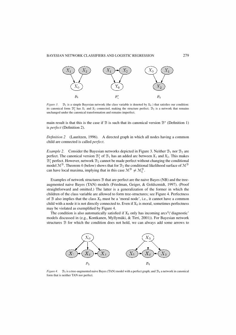
Figure 3. B1 is a simple Bayesian network (the class variable is denoted by X0 ) that satisfies our condition:its canonical form B∗

1 has X1 and X2 connected, making the structure perfect; B2 is a network that remainsunchanged under the canonical transformation and remains imperfect.

main result is that this is the case if B is such that its canonical version B∗ (Definition 1)is perfect (Definition 2).

Definition 2 (Lauritzen, 1996). A directed graph in which all nodes having a commonchild are connected is called perfect.

Example 2. Consider the Bayesian networks depicted in Figure 3. Neither B1 nor B2 areperfect. The canonical version B∗

1 of B1 has an added arc between X1 and X2. This makesB∗

1 perfect. However, network B2 cannot be made perfect without changing the conditionalmodel MB. Theorem 4 (below) shows that for B2 the conditional likelihood surface of MB

can have local maxima, implying that in this case MB �= MBL .

Examples of network structures B that are perfect are the naive Bayes (NB) and the tree-augmented naive Bayes (TAN) models (Friedman, Geiger, & Goldszmidt, 1997). (Proofstraightforward and omitted.) The latter is a generalization of the former in which thechildren of the class variable are allowed to form tree-structures; see Figure 4. Perfectnessof B also implies that the class X0 must be a ‘moral node’, i.e., it cannot have a commonchild with a node it is not directly connected to. Even if X0 is moral, sometimes perfectnessmay be violated as exemplified by Figure 4.

The condition is also automatically satisfied if X0 only has incoming arcs4(‘diagnostic’models discussed in (e.g., Kontkanen, Myllymaki, & Tirri, 2001)). For Bayesian networkstructures B for which the condition does not hold, we can always add some arrows to

Figure 4. B3 is a tree-augmented naive Bayes (TAN) model with a perfect graph; and B4 a network in canonicalform that is neither TAN nor perfect.

280 T. ROOS ET AL.

arrive at a structure B′ for which the condition does hold (for instance, add an arrow fromX1 to X3 in B4 of Figure 4). Therefore, MB is always a subset of a larger model MB′

forwhich the condition holds.

4.2. Main result

We now present our main result stating that the conditional models MB and MBL of a

Bayesian network B and the corresponding logistic regression model respectively, areequivalent if B∗ is perfect:

Theorem 3. If B is such that its canonical version B∗ is perfect, then MB = MBL .

The proof is based on the following proposition:

Proposition 2 (Lauritzen, 1996). Let B be a perfect DAG. A distribution P(X) admitsa factorization of the form (1) with respect to B if and only if it factorizes as

P(X) =∏

c ∈ C

φc(X), (18)

where C is the set of cliques in B and the φc(X) are non-negative functions that depend onX only through the variables in clique c.

Recall that a clique is a fully connected subset of nodes. The set of cliques C appearingin (18) contains both maximal and non-maximal cliques (e.g., consisting of single nodes).

Proof of Theorem 3. We need to show that for an arbitrary parameter vector βB forthe logistic model, there are Bayesian network parameters that index the same distributionas the logistic model. Let θB

xi |paibe the parameters obtained from (17), and define the

normalizing constant Z = ∑x

∏mi=0 θB

xi |pai (x). Define

φi (x) ={

Z−1θBx0|pa0

if i = 0

θBxi |pai

if 1 < i ≤ m.(19)

Consider the joint distribution PZ(X) defined by

PZ (x | θB) =m∏

i=0

φi (x) = 1

Z

m∏i=0

θBxi |pai (x). (20)

Note that, even though the product θBxi |Pai (x) may not sum to one over all data vectors

x, by introducing the normalizing constant Z, we ensure that the resulting PZ (x | θB)defines a probability distribution for (X0, . . . , Xm) . Distribution (20) induces the sameconditionals for X0 as the logistic model with parameter vector βB given by (14). Each


function φi (x) is non-negative and a function of the set {Xi} ∪ Pai , which is a clique byassumption. Thus (20) is a factorization of the form (18) and Proposition 2 implies thatPZ(X) admits a factorization of the form (1) (the usual Bayesian network factorization).Thus there are Bayesian network parameters that satisfy the sum-to-one constraint andrepresent distribution PZ(X). In particular, those parameters give the same conditionaldistributions for X0 as the logistic model. �

The proof is not constructive in that it does not explicitly give the Bayesian networkparameters that give the same conditional distributions as the logistic model. A constructiveproof is given by Wettig et al. (2003). We omitted it here because the present proof is muchshorter, easier to understand and clarifies the connection to perfectness.

Together with Corollary 2 (stating that the conditional log-likelihood is concave),Theorem 3 shows that perfectness of B∗ suffices to ensure that the conditional likelihoodsurface of MB has no local (non-global) maxima. This further implies that, for example,the conditional likelihood surface of TAN models has no local maxima. Therefore, a globalmaximum can be found by local optimization techniques.

But what about the case in which B∗ is not perfect? Our second result, Theorem 4 (provenin the Appendix) says that in this case, there can be local maxima:

Theorem 4. There exist network structures B whose canonical form B∗ is not perfect,and for which the conditional likelihood (6) has local, non-global maxima.

The theorem implies that MBL �= MB for some network structures B. In fact, it implies

the stronger statement that for some structures B, no logistic model indexes the sameconditional distributions as MB. The proof of this stronger statement is by contradiction:if MB coincided with some logistic regression model, the conditional likelihood surface inMB would not have local maxima—contradiction.

Thus, perfectness of B∗ is not a superfluous condition. We may now ask whether it is anecessary condition for having MB′

L = MB for some logistic model MB′L , with a (possibly

different) network structure B′. We plan to address this intriguing open question in futurework.

5. Technical issues

At this point we have all the tools together in order to build a logistic regression modelequivalent to any given Bayesian classifier with underlying network structure B such thatB’s canonical version B∗ is perfect. Its parameters may be determined using hill-climbingor some other local optimization method, such that the conditional log-likelihood is maxi-mized. This results in a prediction method that in most cases outperforms the correspondingBayesian classifier with ordinary maximum likelihood parameters. In practice, however,we find that there is a number of questions yet to be answered. In the following, we addresssome crucial technical details and outline the algorithms implemented.

282 T. ROOS ET AL.

5.1. Standard or logistic parameterization?

Because the mapping from the Bayesian parameters to the logistic model in the proof ofTheorem 2 is continuous, it follows (with some calculus) that if MB = MB

L , then allmaxima of the (concave) conditional likelihood in the logistic parameterization are global(and connected) maxima also in the standard Bayesian parameterization. Thus we may alsoin the standard parameterization optimize the conditional log-likelihood locally to obtain aglobal maximum.

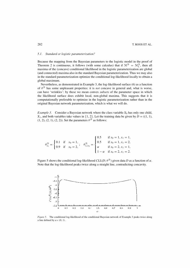
Nevertheless, as demonstrated in Example 3, the log-likelihood surface (6) as a functionof θB has some unpleasant properties: it is not concave in general and, what is worse,can have ‘wrinkles’: by these we mean convex subsets of the parameter space in whichthe likelihood surface does exhibit local, non-global maxima. This suggests that it iscomputationally preferable to optimize in the logistic parameterization rather than in theoriginal Bayesian network parameterization, which is what we will do.

Example 3. Consider a Bayesian network where the class variable X0 has only one child,X1, and both variables take values in {1, 2}. Let the training data be given by D = ((1, 1),(1, 2), (2, 1), (2, 2)). Set the parameters θB as follows:

θBx0

={

0.1 if x0 = 1,

0.9 if x0 = 2,; θB

x1|x0=

0.5 if x0 = 1, x1 = 1,

0.5 if x0 = 1, x1 = 2,

α if x0 = 2, x1 = 1,

1 − α if x0 = 2, x1 = 2.

Figure 5 shows the conditional log-likelihood CLL(D; θB) given data D as a function of α.Note that the log-likelihood peaks twice along a straight line, contradicting concavity.

Figure 5. The conditional log-likelihood of the conditional Bayesian network of Example 3 peaks twice alonga line defined by α ε (0, 1) .


5.2. Continuous predictor variables

Bayesian classifiers have a built-in difficulty in handling continuous data since all condi-tional probability distributions are represented as tables of the form θB

xi |pai, see Section 2.2.

Opposed to that, logistic regression models have no natural way of handling discrete data.But this shortcoming can easily be ironed out by introducing a covariate Yxi ,pai

for eachinstantiation pai of the parent set of a variable Xi as we have seen in Section 3.2.

For our experiments we discretized any continuous features based on the training dataonly, using the entropy-based method of Fayyad and Irani (1993). This way, the methodswe compare will have the same (discrete) input.

Note that logistic models are much more flexible than this and we have not yet exploitedall their advantages. We could have fed them the original continuous values just as well,they would have not had any difficulty in combining this information with that of other,discrete attributes; we could have even handled mixed features (e.g. “died at age” ∈ {alive,0, 1, . . .} etc.). It is also possible to discretize on the fly, i.e. to generate covariates of theform Y≤xi := I[Xi ≤xi ] as this seems beneficial for the discriminative model. One might evenuse a combination of the original continuous value of a feature and its discretized versionby introducing a piece-wise log-linear function into the model. We leave the pursuit ofthese ideas as an objective for future research.

5.3. Model selection

Usually we are not provided with a Bayesian network structure B, but we are only givena data sample D, and somehow must choose a model (structure) B ourselves. How shouldwe do this? This is a hard problem already when modelling the joint data distribution(Buntine, 1994; Heckerman, 1996; Myllymaki et al., 2002). Finding a good conditionalmodel can be much harder than joint modelling, and many of the tools for modelling thejoint distribution can no longer be used. For example, methods such as cross-validation orprequential validation become computationally highly demanding, since for each candidatenetwork one has to re-optimize the model parameters. While optimizing the conditionallog-likelihood of a single model is quite feasible for reasonable size data, optimizationseems too computationally demanding for the task of model selection. Using the joint datalikelihood as a criterion is easier but may yield very poor results, while improvementshave been achieved with heuristic ‘semi-supervised’ methods that mix supervised andunsupervised learning (Keogh & Pazzani, 1999; Kontkanen et al., 1999; Cowell, 2001;Shen et al., 2003; Madden, 2003; Raina et al., 2003; Grossman & Domingos, 2004).

For these reasons, we take a different approach. We start out with the naive Bayesclassifier, the simplest model taking into account all data entries given. Our predictions areof the form (14), extended by independence. Since for naive Bayes models, the set pa+

iis empty for all nodes Xi, we may denote βx0 := βx0,pa0(x) and βx0,xi := βx0,xi ,pa+

0 (x). Thisbecomes our first algorithm, conditional naive Bayes (cNB). Our second algorithm, prunednaive Bayes (pNB) will become a submodel of cNB, with a parameter selection schemeas described below. Both the cNB and the pNB models are parameterized in the logisticregression fashion.

284 T. ROOS ET AL.

We stress that the scope of our experiments is rather limited. Implementing a fullysupervised, yet computationally feasible model selection method without severe restrictionson the range of network structures is a challenging open research topic.

5.4. Missing data

Most standard classification methods—including Bayesian network classifiers and logisticregression—have been designed for the case where all training data vectors are complete,in the sense that they have no missing values. Yet in real-world data, missing data (featurevalues) appear to be the rule than the exception. Therefore we need to explicitly deal withthis problem. The most general way of handling the issue is to treat ‘missing’ as a legitimatevalue for all features Xi whose value is missing in one or more data vectors (Myllymakiet al., 2002). This however, makes our model larger and thus may result in more overfitting,and therefore worse classification performance for small samples.

Instead, it is often assumed that the patterns of ‘missingness’ in the data do not provideany information about the class values. Mathematically, this can be expressed as follows:we assume that the true data generating distribution satisfies, for all class values x0, allvectors x−i with the ith element missing,

P(x0 | x−i , xi = ‘missing’) =∑

xi

P(xi | x−i )P(x0 | x), (21)

where the sum is over all ‘ordinary’ values for Xi (excluding the value‘missing’). The sameequation can be trivially extended to multiple missing values in x.

While the assumption (21) is typically wrong, it often leads to acceptable results inpractice. The related notion of ‘missing completely at random’ (MCAR) (see e.g. Little &Rubin, 1987) is a strictly stronger requirement since it requires that xi being missing givesno information about the joint distribution of (X0, . . . , XM), whereas we only require thisto hold for the class variable X0.

The proper way to implement (21) would to integrate out the missing entries. However,this makes the parameter learning (search) problem NP-complete. Therefore, we adjustedour learning method so as to achieve an approximation of (21), by effectively ignoring(‘skipping’) parameters corresponding to missing information, during both inference andprediction. More precisely, we introduce constraints of the form

∑xi

P(xi | x−i )βx0,i = 0, (22)

where we estimate the terms P(xi | x−i ) from the training data. As a result, our modelswill respect an approximation to (21), namely its logarithmic version

log P(x0 | x−i , xi = ‘missing’, β) =∑

xi

P(xi | x−i ) log P(x0 | x, β), (23)


This way, skipping all parameters corresponding to missing values results in logarithmicallyunbiased predictive distributions, which judged on the basis of our experiments reported inSection 6 seems to be a good enough approximation in practice.

5.5. Priors

In practical applications, a sample D will typically include zero frequencies, i.e. n[x0,xi ] = 0for some x0, xi. In that case, the conditional log-likelihood CLL(D; β) given by (16) willhave no maximum over β, but some βx0,xi will diverge to −∞. The same problem can arisein more subtle situations as well, see Example 4 in Wettig et al. (2002).

We can avoid such problems by introducing a Bayesian prior distribution on the con-ditional model B (Bernardo & Smith, 1994). Kontkanen et al. (2000) have shown that forordinary, unsupervised naive Bayes, whenever we are in danger of over-fitting the trainingdata—usually with small sample sizes—prediction performance can be greatly improvedby imposing a prior on the parameters. Since the conditional model cNB is inclined toworse over-fitting than unsupervised naive Bayes (Ng & Jordan, 2001), this should holdalso in our case.

We impose a strictly concave prior that goes to zero as the absolute value of any parameterapproaches infinity. We choose the closest we can find to the uniform, least informativeprior in the usual parameterization where parameters take values between zero and one. Weretransform the parameters βx0 and βx0,xi back into the space of probability distributions(by taking their normalized exponentials) and define their prior probability density, P(β),to be proportional to the product of all entries in the resulting distributions.

Instead of the conditional log-likelihood CLL we optimize the ‘conditional posterior’(Grunwald et al., 2002):

CLL+(D; β) := CLL(D; β) + ln P(β). (24)

Using this prior also yields strict concaveness of CLL+ as the sum of a concave and astrictly concave function, which guarantees a unique maximum.

5.6. Algorithms

We now fill in the missing details of our algorithms, and explain how the actual optimiza-tion is performed. The conditional naive Bayes algorithm maximizes CLL+(D; β) usingcomponent-wise binary search until convergence. Although we can compute all first andsecond derivatives, (9) and (10), we found that this takes so much computation time thatthe benefit in convergence speed obtained by using more sophisticated methods such asNewton-Raphson or conjugate gradient ascent is lost. Minka (2001) suggests and comparesa number of algorithms for this task. In our case the simplest of them, coordinate-wise linesearch, seems to suffice.

Our second method, the pruned naive Bayes classifier pNB aims at preventing over-fitting. We prune the full naive Bayes model cNB by maximizing the same objective but

286 T. ROOS ET AL.

with the additional freedom to exclude some parameters from the model. These are beingignored in the same way any parameter is when the corresponding data entry is missing:

CLL+(D; β) = ∑j ln

(exp

(βx0 +∑

i :βx0 ,x

ji

∈β j βx0 ,x

ji

)∑n0

x ′0=1

exp(βx ′

0+∑

i :βx ′0 ,x

ji

∈β j βx ′0 ,x

ji

))

+ ln P(β), (25)

where β j is defined to be the set of parameters that apply to vector x j : β j := {βx0,xi ∈β: x j

i �= ‘missing′}.Note that although zero valued parameters have no effect on the conditional likelihood,

the corresponding prior term is not zero, so that any parameter that is chosen to be part ofthe model has an associated cost to it. This defines a natural threshold: a parameter βx0,xi

that does not improve the conditional log-likelihood by at least −ln P(βx0,xi ) ≥ −ln P(0)will be removed from the model, since it will deteriorate the log-posterior.

The pNB algorithm is quite simple. We start out with the full cNB model and eliminateparameters one at a time until no improvement is achieved. To speed up the process, wechoose the next parameter to be dropped so that CLL+(D; β) is maximized without re-optimizing the remaining parameters. We re-optimize only after choosing which parameterto drop. When there is no parameter left whose exclusion from the model yields directgain, we choose the parameter causing the least loss. If after re-optimizing the system theobjective still has not improved, we undo the last step and the algorithm terminates.

6. Empirical results

We compare our methods against conventional naive Bayes and against each other. Ourexperimental methodology resembles that of Madden (2003) and Friedman, Geiger, andGoldszmidt (1997). We split each data set into disjunct train and test sets at random suchthat the training set contains 80% of the original data set and the test set the remaining 20%. This we do 20 times independently of the previous splits. We report average log-loss and0/1 loss +/− 1.645 times standard deviation over splits.

As mentioned in Section 5.1, we discretize continuous features using the entropy-basedmethod of Fayyad and Irani (1993). This is done using the training data only, so that foreach random split this results in possibly different discretizations. Data vectors with missingentries were included in the tests. As a test bed we took 18 data sets from the UCI MachineLearning Repository (Blake & Merz, 1998), ten of which contain missing data. In the tablesbelow, these are marked by an asterisk ‘ ∗ ’.

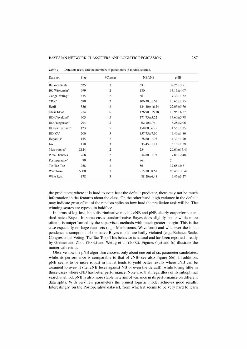
Table 1 lists the data sets used, their sizes and the number of parameters used bythe different algorithms. The NB and cNB models, although parameterized differently,obviously contain the same number of parameters. Variance in this number is due toindividual discretizations on each training set. Note the drastic pruning performed by pNB.

We list the log-scores achieved by the algorithms NB, cNB and pNB in Table 2. Forcomparison we also report the results of the default predictor (class node independent ofeverything else) which—as also the NB algorithm—has been equipped with a uniformprior on its parameters. The default gives some clue about how hard it is to learn from


Table 1. Data sets used, and the numbers of parameters in models learned.

Data set Size #Classes NB/cNB pNB

Balance Scale 625 3 63 32.25±3.81

BC Wisconsin∗ 699 2 180 13.15±4.07

Congr. Voting∗ 435 2 66 7.30±1.32

CRX∗ 690 2 106.30±1.61 10.65±1.95

Ecoli 336 8 124.40±16.24 22.05±5.76

Glass Ident. 214 6 126.90±15.78 16.95±6.57

HD Cleveland∗ 303 5 171.75±5.52 14.60±5.78

HD Hungarian∗ 294 2 62.10±.74 8.25±2.06

HD Switzerland∗ 123 5 158.00±6.75 4.55±1.25

HD VA∗ 200 5 157.75±7.30 6.40±1.80

Hepatitis∗ 155 2 78.80±1.97 4.30±1.70

Iris 150 3 33.45±1.81 5.10±1.59

Mushrooms∗ 8124 2 234 29.00±15.40

Pima Diabetes 768 2 34.80±1.97 7.80±2.48

Postoperative∗ 90 4 96 2

Tic-Tac-Toe 958 2 56 37.65±0.81

Waveform 5000 3 215.70±8.61 96.40±30.49

Wine Rec. 178 3 88.20±6.48 9.45±3.27

the predictors; where it is hard to even beat the default predictor, there may not be muchinformation in the features about the class. On the other hand, high variance in the defaultmay indicate great effect of the random splits on how hard the prediction task will be. Thewinning scores are typeset in boldface.

In terms of log-loss, both discriminative models cNB and pNB clearly outperform stan-dard naive Bayes. In some cases standard naive Bayes does slightly better while moreoften it is outperformed by the supervised methods with much greater margin. This is thecase especially on large data sets (e.g., Mushrooms, Waveform) and whenever the inde-pendence assumptions of the naive Bayes model are badly violated (e.g., Balance Scale,Congressional Voting, Tic-Tac-Toe). This behavior is natural and has been reported alreadyby Greiner and Zhou (2002) and Wettig et al. (2002). Figures 6(a) and (c) illustrate thenumerical results.

Observe how the pNB algorithm chooses only about one out of six parameter candidates,while its performance is comparable to that of cNB; see also Figure 6(e). In addition,pNB seems to be more robust in that it tends to yield better results where cNB can beassumed to over-fit (i.e. cNB loses against NB or even the default), while losing little inthose cases where cNB has better performance. Note also that, regardless of its suboptimalsearch method, pNB is also more stable in terms of variance in its performance on differentdata splits. With very few parameters the pruned logistic model achieves good results.Interestingly, on the Postoperative data-set, from which it seems to be very hard to learn

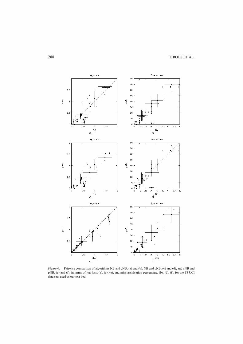
288 T. ROOS ET AL.

Figure 6. Pairwise comparison of algorithms NB and cNB, (a) and (b), NB and pNB, (c) and (d), and cNB andpNB, (e) and (f), in terms of log-loss, (a), (c), (e), and misclassification percentage, (b), (d), (f), for the 18 UCIdata sets used as our test bed.


Table 2. Predictive accuracies with respect to logarithmic loss.

Data set Default NB cNB pNB

Balance Scale .925±.057 .528±.078 .214±.067 .228±.081

BC Wisconsin∗ .646±.047 .261±.195 .140±.078 .113±.050

Congr. Voting∗ .675±.033 .577±.359 .112±.081 .121±.064

CRX∗ .688±.012 .396±.134 .332±.099 .339±.078

Ecoli 1.545±.149 .448±.227 .445±.236 .488±.214

Glass Ident. 1.546±.181 .828±.271 .784±.184 .937±.222

HD Cleveland∗ 1.304±.185 1.023±.322 1.125±.350 1.053±.232

HD Hungarian∗ .647±.041 .403±.226 .366±.128 .407±.211

HD Switzerland∗ 1.392±.157 1.468±.299 1.652±.349 1.367±.149

HD VA∗ 1.542±.074 1.500±.166 1.613±.207 1.544±.135

Hepatitis∗ .532±.160 .434±.296 .409±.267 .413±.177

Iris 1.110±.018 .091±.123 .112±.091 .111±.075

Mushrooms∗ .693±.001 .129±.029 .001±.001 .002±.001

Pima Diabetes .647±.036 .433±.059 .442±.043 .456±.041

Postoperative∗ .714±.213 .808±.310 .927±.337 .707±.219

Tic-Tac-Toe .650±.029 .554±.045 .090±.030 .090±.030

Waveform 1.099±.001 .634±.082 .296±.027 .299±.025

Wine Rec. 1.104±.048 .014±.034 .028±.033 .053±.051

anything about its class, pNB constantly chooses only two parameters which leads to betterperformance than using the full model. On the other hand, for data-set Tic-Tac-Toe, pNBchooses a large fraction of the available parameters behaving no different from cNB on allsplits.

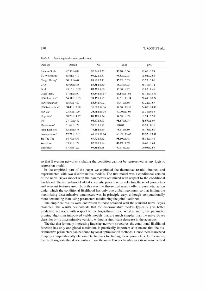
Table 3 is the counterpart of Table 2, reporting the results of the same test runs in terms of0/1-loss. Figures 6(b), (d) and (f) compare the classification errors of the three algorithms.Naive Bayes seems to do relatively better under the 0/1-loss, but note that again it wins bysmaller margins than those it loses by on other data sets. The logistic models cNB and pNBare quite comparable also in terms of classification accuracy.

7. Conclusions

The focus of this paper is in discriminative learning of models from sample data, wherethe goal is to determine the model parameters maximizing the conditional (supervised)likelihood instead of the commonly used joint (unsupervised) likelihood. In the theoreticalpart of the paper we showed that for Bayesian network models satisfying a simple graph-theoretic condition, this problem is equivalent to a logistic regression problem. Bayesiannetwork structures satisfying this condition include the naive Bayes model and the tree-augmented naive Bayes model, but the condition allows also other non-trivial networkstructures. It remains an interesing open problem whether the condition is also necessary

290 T. ROOS ET AL.

Table 3. Percentages of correct predictions.

Data set Default NB cNB pNB

Balance Scale 42.36±4.08 90.24±3.27 93.20±3.56 92.60±3.98

BC Wisconsin∗ 65.61±7.19 97.22±1.87 95.82±2.03 95.04±2.68

Congr. Voting∗ 60.12±6.44 89.89±5.71 95.92±3.33 95.75±3.01

CRX∗ 55.65±5.35 87.36±4.30 85.98±4.93 85.11±4.12

Ecoli 43.16±10.09 85.29±8.60 85.00±8.22 82.87±8.46

Glass Ident. 31.51±8.90 69.54±11.57 69.54±11.64 65.12±13.93

HD Cleveland∗ 54.51±10.85 58.77±9.87 58.61±11.54 58.69±10.74

HD Hungarian∗ 65.59±7.89 85.34±7.02 84.41±6.56 83.22±7.67

HD Switzerland∗ 38.40±12.88 36.00±14.16 34.60±13.55 34.00±14.40

HD VA∗ 23.50±10.54 33.75±13.04 30.00±13.07 25.38±9.83

Hepatitis∗ 78.23±11.27 86.78±8.24 84.68±9.09 81.94±9.95

Iris 27.17±5.42 95.67±5.93 95.67±5.07 95.67±5.07

Mushrooms∗ 51.69±1.78 95.51±0.92 100.00 99.98±0.11

Pima Diabetes 65.26±5.73 79.16±4.69 78.51±3.89 78.15±3.61

Postoperative∗ 72.22±13.91 68.89±11.64 63.89±13.43 72.22±13.91

Tic-Tac-Toe 64.79±4.57 69.72±4.42 98.10±1.48 98.10±1.48

Waveform 33.50±1.79 82.20±1.84 86.69±1.69 86.60±1.68

Wine Rec. 37.36±12.71 99.58±1.68 99.17±2.15 99.03±2.69

so that Bayesian networks violating the condition can not be represented as any logisticregression model.

In the empirical part of the paper we exploited the theoretical results obtained andexperimented with two discriminative models. The first model was a conditional versionof the naive Bayes model with the parameters optimized with respect to the conditionallikelihood. The second model added a heuristic procedure for selecting the set of parametersand relevant features used. In both cases the theoretical results offer a parameterizationunder which the conditional likelihood has only one global maximum so that finding themaximizing discriminative parameters was in principle easy, although computationallymore demanding than using parameters maximizing the joint likelihood.

The empirical results were contrasted to those obtained with the standard naive Bayesclassifier. The results demonstrate that the discriminative models typically give betterpredictive accuracy with respect to the logarithmic loss. What is more, the parameterpruning algorithm introduced yields models that are much simpler than the naive Bayesclassifier or its discriminative version, without a significant decrease in the accuracy.

The fact that for many interesting Bayesian network structures, the conditional likelihoodfunction has only one global maximum, is practically important as it means that the dis-criminative parameters can be found by local optimization methods. Hence there is no needto apply computationally elaborate techniques for finding these parameters. Furthermore,the result suggests that if one wishes to use the naive Bayes classifier as a straw man method


to which alternative approaches are to be compared, as is often the case, one could equallywell use an even better straw man method offered by the supervised version of the naiveBayes model.

On the other hand, the results may have implications with respect to the model selectionproblem in supervised domains: many model selection criteria typically contain the datalikelihood as one of the factors of the criterion—cf. for example, the Bayesian InformationCriterion (BIC) (Schwarz, 1978) or approximations of the Minimum Description Length(MDL) criterion (Rissanen, 1996). Therefore, it is natural to assume that the conditionallikelihood plays an important role in the supervised versions of the model selection criteria.This aspect will be addressed more formally in our future work.

A. Appendix: Proofs

Proof (sketch) of Theorem 4: Use the rightmost network in Figure 3 with structureX0 → X2 ← X1. Let the data be

D = ((1, 1, 1), (1, 1, 2), (2, 2, 1), (2, 2, 2)). (26)

We are interested in predicting the value of X0 given X1 and X2. The parameter definingthe distribution of X1 has no effecton conditional predictions and we can ignore it. For theremaining five parameters we use the following notation:

θ2 := P(X0 = 2),θ2|1,1 := P(X2 = 2 | X0 = 1, X1 = 1),θ2|1,2 := P(X2 = 2 | X0 = 1, X1 = 2),θ2|2,1 := P(X2 = 2 | X0 = 2, X1 = 1),θ2|2,2 := P(X2 = 2 | X0 = 2, X1 = 2).

(27)

Idea of the Proof. In the empirical distribution based on data D, X0 is highly (even perfectly)dependent on X1, even given the value of X2. Such a perfect dependence cannot berepresented by any of the distributions in MB since the network structure implies thatconditioned on X2, X1 and X0 must be independent. However, the parameters θ2|1,2 andθ2|2,1 correspond to contexts that do not occur in D and this fact can be exploited: by settingθ2|2,1 to 0 and θ2|1,2 to 0, we can represent distributions θ with P(X0 = X1 | X2 = 2, θ ) = 1and P(X0 = X1 | X2 = 1, θ ) = 0.5 ± ε for any ε > 0. These distributions represent someof the dependence between X0 and X1 after all and, for ε → 0, converge to the maximumconditional likelihood. However, by setting θ ′

2|2,1 to 1 and θ ′2|1,2 to 1, we can represent

distributions θ with P(X0 = X1 | X2 = 1, θ ′) = 1 and P(X0 = X1 | X2 = 2, θ ′) = 0.5±ε

which also converge to the maximum conditional likelihood as ε → 0. In Part I of the proofwe formalize this argument and show that with data (26), there are four non-connectedsuprema of the conditional likelihood. In Part II, we sketch how the argument can beextended to allow for non-global maxima (rather than suprema).

292 T. ROOS ET AL.

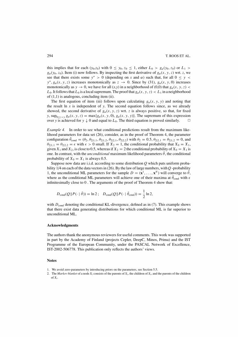
Figure 7. Function g (x, y, z) given by (29) with x = 0.5.

Part I. The conditional log-likelihood can be written as

CLL(D; θB) = g(1 − θ2, θ2|1,1, θ2|2,1) + g(θ2, θ2|2,2, θ2|1,2), (28)

where

g(x, y, z) := f (x, y, z) + f (x, 1 − y, 1 − z), (29)

and

f (x, y, z) := lnxy

xy + (1 − x)z. (30)

Figure 7 illustrates function g(x,y,z) at x = 0.5. In (28) each parameter except θ2 appearsonly once. Thus, for a fixed θ2 we can maximize each term separately. We can now applyLemma 3 below with α = 1/2, so that gα(x, y, z) = 2g(x, y, z) for the g defined in(29). It follows from the lemma that the supremum of the log-likelihood with θ2 fixed isln(1−θ2)+ ln(θ2), which achieves its maximum value −2 ln 2 at θ2 = 0.5. Furthermore, thelemma shows that the log-likelihood approaches its supremum when θ2|2,1 ∈ {0, 1}, θ2|1,2 ∈{0, 1}, θ2|1,1 → θ2|2,1, and θ2|2,2 → θ2|1,2. Moreover, by item (ii) of the lemma, thesesuprema are separated by areas where the log-likelihood is smaller, i.e., the suprema arelocal and not connected.Part II. To conclude the proof we still need to address two issues: (a) the four local supremagive the same conditional log-likelihood −2 ln 2, and (b), they are suprema, not maxima(not achieved by any θB). We now roughly sketch how to extend the argument to deal withthese issues. Concerning (a), fix some 0 < α < 1 and consider a sample D′ consisting ofN data vectors, with αN/2 repetitions of (1,1,1), αN/2 repetitions of (2,2,1), (1 − α)N/2repetitions of (1,1,2) and (1 − α)N/2 repetitions of (2,2,2). Using Lemma 3 in the sameway as before, we find that the conditional log-likelihood has four local suprema which arenot connected. Moreover, if α �= 1/2, then at least two of these suprema are not equal.

Concerning (b), let D′′ be the sample D′ but with four extra ‘barrier’ datavectors (1,2,1),(2,1,1),(1,2,2),(2,1,2) added. Let C ′′ be the corresponding condi-tional log-likelihood, C ′′(θB) := C L L(D′′; θB). If one of the five parameters


θ2, θ2|1,1, θ2|2,1, θ2|2,2, θ2|1,2 ∈ {0, 1}, then C ′′(θB) = −∞. On the other hand, C ′′ iscontinuous and finite for (θ2, θ2|1,1, θ2|2,1, θ2|2,2, θ2|1,2) ∈ (0, 1)5, so C ′′ must achieve itsmaximum or maxima for each N. On the other hand, for large N, the influence of the barrierdata vectors C ′′ at each individual point θB becomes negligible. Using Lemma 3, item (iii),these two facts can be exploited to show that for large N, C ′′ has (at least) two maxima,which, if α �= 1/2, are neither equal nor connected. We omit further details. �

Lemma 3. Define gα(x, y, z) := α f (x, y, z) + (1 − α) f (x, 1 − y, 1 − z), wheref (x, y, z) is defined as in (30). Fix some 0 < x < 1 and 0 < α < 1. With y and zboth varying between 0 and 1, we have:(i) The global supremum of gα(x, y, z) satisfies

sup0≤y,z≤1

gα(x, y, z) = sup{α ln x, (1 − α) ln x}.

(ii) The local suprema are at z = 0, y ↓ 0 and at z = 1, y ↑ 1:

limy↓0

gα(x, y, 0) = (1 − α) ln x ; limy↑1

gα(x, y, 1) = α ln x .

(iii) For restricted z we have:

sup0≤y,z≤1,z=y gα(x, y, z) = ln xsup0≤y,z≤1,z<y gα(x, y, z) = (1 − α) ln xsup0≤y,z≤1,z>y gα(x, y, z) = α ln x .

Proof Differentiating twice wrt. z gives

∂2

∂2zgα(x, y, z) = α(1 − x)2

(xy + (1 − x)z)2+ (1 − α)(1 − x)2

(x(1 − y) + (1 − x)(1 − z))2,

which is always positive and the function achieves its maximum value either at z = 0 orz = 1 or both. At these two points differentiating wrt. y yields

∂

∂ygα(x, y, 0) = (1 − α)(x − 1)

(1 − y)(1 − xy);

∂

∂ygα(x, y, 1) = α(1 − x)

y(xy + 1 − x). (31)

Since in the first case the derivative is always negative, and in the second case the derivativeis always positive, gα(x, y, 0) increases monotonically as y → 0, and gα(x, y, 1) increasesmonotonically as y → 1. Denoting

L0 = limy↓0

gα(x, y, 0) = (1 − α) ln x and L1 = limy↑1

gα(x, y, 1) = α ln x,

294 T. ROOS ET AL.

this implies that for each (y0,z0) with 0 ≤ y0, z0 ≤ 1, either L0 > gα(y0, z0) or L1 >

gα(y0, z0). Item (i) now follows. By inspecting the first derivative of gα(x, y, z) wrt. z, wesee that there exists some y∗ > 0 (depending on x and α) such that, for all 0 ≤ y <

y∗, gα(x, y, z) increases monotonically as z → 0. Since by (31), gα(x, y, 0) increasesmonotonically as y → 0, we have for all (x,y) in a neighborhood of (0,0) that gα(x, y, z) <

L0. It follows that L0 is a local supremum. The proof that gα(x, y, z) < L1 in a neighborhoodof (1,1) is analogous, concluding item (ii).

The first equation of item (iii) follows upon calculating gα(x, y, y) and noting thatthe result ln x is independent of y. The second equation follows since, as we alreadyshowed, the second derivative of gα(x, y, z) wrt. z is always positive, so that, for fixedy, sup0≤z<y gα(x, y, z) = max{gα(x, y, 0), gα(x, y, y)}. The supremum of this expressionover y is achieved for y ↓ 0 and equal to L0. The third equation is proved similarly. �

Example 4. In order to see what conditional predictions result from the maximum like-lihood parameters for data set (26), consider, as in the proof of Theorem 4, the parameterconfiguration θcond = (θ2, θ2|1,1, θ2|1,2, θ2|2,1, θ2|2,2) with θ2 = 0.5, θ2|2,1 = θ2|1,2 = 0, andθ2|1,1 = θ2|2,2 = ε with ε > 0 small. If X2 = 1, the conditional probability that X0 = X1,given X1 and X2, is close to 0.5, whereas if X2 = 2 the conditional probability of X0 = X1 isone. In contrast, with the unconditional maximum likelihood parameters θ , the conditionalprobability of X0 = X1 is always 0.5.

Suppose now data are i.i.d. according to some distribution Q which puts uniform proba-bility 1/4 on each of the data vectors in (26). By the law of large numbers, with Q -probability1, the unconditional ML parameters for the sample D = (x1, . . . , xN ) will converge to θ ,where as the conditional ML parameters will achieve one of their maxima at θcond with ε

infinitesimally close to 0 . The arguments of the proof of Theorem 4 show that:

Dcond(Q‖P(· | θ )) = ln 2 ; Dcond(Q‖P(· | θcond)) = 1

2ln 2,

with Dcond denoting the conditional KL-divergence, defined as in (7). This example showsthat there exist data generating distributions for which conditional ML is far superior tounconditional ML.

Acknowledgments

The authors thank the anonymous reviewers for useful comments. This work was supportedin part by the Academy of Finland (projects Cepler, DeepC, Minos, Prima) and the ISTProgramme of the European Community, under the PASCAL Network of Excellence,IST-2002-506778. This publication only reflects the authors’ views.

Notes

1. We avoid zero-parameters by introducing priors on the parameters, see Section 5.5.2. The Markov blanket of a node Xi consists of the parents of Xi, the children of Xi, and the parents of the children

of Xi.


3. The addition can always be done without introducing any cycles (Lauritzen, 1996), usually in several differentways all of which are equivalent for our purposes.

4. As noted in Section 2, in that case the maximum conditional likelihood parameters may even be determinedanalytically.

References

Barndorff-Nielsen, O. (1978). Information and exponential families in statistical theory. New York, NY: JohnWiley & Sons.

Bernardo, J. & Smith, A. (1994). Bayesian theory. New York, NY: John Wiley & Sons.Bishop, C. (1995). Neural networks for pattern recognition. Oxford, UK: Oxford University Press.Blake, C., & Merz, C. (1998). UCI repository of machine learning databases. http://www.ics.uci.edu/∼mlearn/

MLRepository.html. University of California, Irvine, Department of Information and Computer Science.Buntine, W. (1994). Operations for learning with graphical models. Journal of Artificial Intelligence Research,

2, 159–225.Cowell, R. (2001). On searching for optimal classifiers among Bayesian networks. In T. Jaakkola, & T. Richardson

(Eds.), Proceedings of the eight international workshop on artificial intelligence and statistics. (pp. 175–180).San Francisco, CA: Morgan Kaufmann.

Dawid, A. (1976). Properties of diagnostic data distributions. Biometrics, 32:3, 647–658.Dempster, A., Laird, N., & Rubin, D. (1977). Maximum likelihood from incomplete data via the EM algorithm.

Journal of the Royal Statistical Society, Series B, 39:1, 1–38.Fayyad, U., & Irani, K. (1993). Multi-interval discretization of continuous-valued attributes for classification

learning. In R. Bajcsy (Ed.), Proceedings of the thirteenth international joint conference on artificial intelligence(pp. 1022–1027). San Francisco, CA: Morgan Kaufmann.

Friedman, N., Geiger, D., & Goldszmidt, M. (1997). Bayesian network classifiers. Machine Learning, 29:2,131–163.

Greiner, R., Grove, A., & Schuurmans, D. (1997). Learning Bayesian nets that perform well. In D. Geiger, & P.P. Shenoy (Eds.), Proceedings of the thirteenth annual conference on uncertainty in artificial intelligence (pp.198–207). San Francisco, CA: Morgan Kaufmann.

Greiner, R., & Zhou, W. (2002). Structural extension to logistic regression: discriminant parameter learning ofbelief net classifiers. In R. Dechter, M. Kearns, & R. Sutton (Eds.), Proceedings of the eighteenth nationalconference on artificial intelligence (pp. 167–173). Cambridge, MA: MIT Press.

Grossman, D., & Domingos, P. (2004). Learning Bayesian network classifiers by maximizing conditional likeli-hood. In C. E. Brodley (Ed.), Proceedings of the twenty-first international conference on machine learning (pp.361–368). Madison, WI: Omnipress.

Grunwald, P., Kontkanen, P., Myllymaki, P., Roos, T., Tirri, H., & Wettig, H. (2002). Supervised posteriordistributions. Presented at the seventh Valencia international meeting on Bayesian statistics, Tenerife, Spain.

Heckerman, D. (1996). A tutorial on learning with Bayesian networks. Technical Report MSR-TR-95-06, Mi-crosoft Research, Redmond, WA.

Heckerman, D., & Meek, C. (1997a). Embedded Bayesian network classifiers. Technical Report MSR-TR-97-06,Microsoft Research, Redmond, WA.

Heckerman, D., & Meek, C. (1997b). Models and selection criteria for regression and classification. In D. Geiger,& P.P. Shenoy (Eds.), Proceedings of the thirteenth annual conference on uncertainty in artificial intelligence(pp. 198–207). San Francisco, CA: Morgan Kaufmann.

Jebara, T. (2003). Machine learning: Discriminative and generative. Boston, MA: Kluwer Academic Publishers.Keogh, E., & Pazzani, M. (1999). Learning augmented Bayesian classifiers: A comparison of distribution-based

and classification-based approaches. In D. Heckerman, & J. Whittaker (Eds.), Proceedings of the seventhinternational workshop on artificial intelligence and statistics (pp. 225–230). San Francisco, CA: MorganKaufmann.

Kontkanen, P., Myllymaki, P., Silander, T., & Tirri, H. (1999). On supervised selection of Bayesian networks.In K. B. Laskey, & H. Prade (Eds.), Proceedings of the fifteenth international conference on uncertainty inartificial intelligence (pp. 334–342). San Francisco, CA: Morgan Kaufmann Publishers.

296 T. ROOS ET AL.

Kontkanen, P., Myllymaki, P., Silander, T., Tirri, H., & Grunwald, P. (2000). On predictive distributions andBayesian networks. Statistics and Computing, 10:1, 39–54.

Kontkanen, P., Myllymaki, P., & Tirri, H. (2001). Classifier learning with supervised marginal likelihood. In J. S.Breese, & D. Koller (Eds.), Proceedings of the seventeenth conference on uncertainty in artificial intelligence(pp. 277-284). San Francisco, CA: Morgan Kaufmann.

Lauritzen, S. (1996). Graphical models. Oxford, UK: Oxford University Press.Little, R. & Rubin, D. (1987). Statistical analysis with missing data. New York, NY: John Wiley & Sons.Madden, M. (2003). The performance of Bayesian network classifiers constructed using different techniques.

In Working notes of the ECML/PKDD-03 workshop on probabilistic graphical models for classification(pp. 59–70).

McLachlan, G. (1992). Discriminant analysis and statistical pattern recognition. New York, NY: John Wiley &Sons.

McLachlan, G. & Krishnan, T. (1997). The EM algorithm and extensions. New York, NY: John Wiley & Sons.Minka, T. (2001). Algorithms for maximum-likelihood logistic regression. Technical Report 758, Carnegie Mellon

University, Department of Statistics. Revised Sept. 2003.Myllymaki, P., Silander, T., Tirri, H., & Uronen, P. (2002). B-Course: a web-based tool for Bayesian and causal

data analysis. International Journal on Artificial Intelligence Tools, 11:3, 369–387.Ng, A. & Jordan, M. (2001). On discriminative vs. generative classifiers: A comparison of logistic regression

and naive Bayes. In T. G. Dietterich, S. Becker, & Z. Ghahramani (Eds.), Advances in neural informationprocessing systems, 14 (pp. 605–610). Cambridge, MA: MIT Press.

Pearl, J. (1987). Evidential reasoning using stochastic simulation of causal models. Artificial Intelligence, 32:2,245–258.

Pearl, J. (1988). Probabilistic reasoning in intelligent systems: Networks of plausible inference. San Mateo, CA:Morgan Kaufmann.

Raina, R., Shen, Y., Ng, A. Y., & McCallum, A. (2003). Classification with hybrid generative/discriminativemodels. In S. Thrun, L. Saul , & B. Scholkopf (Eds.), Advances in neural information processing systems 16.Cambridge, MA: MIT Press.

Rissanen, J. (1996). Fisher information and stochastic complexity. IEEE Transactions on Information Theory,42:1, 40–47.

Russell, S., Binder, J., Koller, D., & Kanawaza, K. (1995). Local learning in probabilistic networks with hiddenvariables. In S. Thrun, & T. M. Mitchell (Eds.), Proceedings of the fourteenth international joint conference onartificial intelligence (pp. 1146–1152). San Francisco, CA: Morgan Kaufmann Publishers.

Schwarz, G. (1978). Estimating the dimension of a model. Annals of Statistics, 6:2, 461–464.Shen, B., Su, X., Greiner, R., Musilek, P., & Cheng, C. (2003). Discriminative parameter learning of general

Bayesian network classifiers. In Proceedings of the fifteenth IEEE international conference on tools withartificial intelligence (pp. 296–305). Los Alamitos, CA: IEEE Computer Society Press.

Thiesson, B. (1995). Accelerated quantification of Bayesian networks with incomplete data. In U. M. Fayyad,& R. Uthurusamy (Eds.), Proceedings of the first international conference on knowledge discovery and datamining (pp. 306–311). Cambridge, MA: MIT Press.

Wettig, H., Grunwald, P., Roos, T., Myllymaki, P., & Tirri, H. (2002). Supervised naive Bayes parameters. In P.Ala-Siuru, & S. Kaski (Eds.), Proceedings of the tenth Finnish artificial intelligence conference (pp. 72–83).Oulu, Finland: Finnish Artificial Intelligence Society.

Wettig, H., Grunwald, P., Roos, T., Myllymaki, P., & Tirri, H. (2003). When discriminative learning of Bayesiannetwork parameters is easy. In G. Gottlob, & T. Walsh (Eds.), Proceedings of the eighteenth international jointconference on artificial intelligence (pp. 491–496). San Francisco, CA: Morgan Kaufmann Publishers.

Received March 5, 2004Revised November 26, 2004Accepted November 26, 2004

on discriminative bayesian network classifiers and logistic

Documents