on applications of xfem to dynamic fracture and dislocations

On Applications of XFEM to DynamicFracture and Dislocations

Ted Belytschko1, Jeong-Hoon Song2, Hongwu Wang3, and Robert Gracie4

Summary. The application of the extended finite element method, which canmodel arbitrary discontinuities in finite elements to dynamic fracture and dislo-cations, is described. The dynamic fracture methodology is applied to a problem ofcrack branching and compared to element deletion and interelement crack methods.The dislocation method directly models the dislocation as a tangential discontinuity.This makes the method readily applicable to problems with interfaces and aniso-tropy.

Key words: extended finite element method; dynamic fracture; dislocations

We describe some recent studies in the extended finite element method(XFEM) and related methods for the treatment of dynamic crack propagationand a new approach for treating dislocations by XFEM. The extended finiteelement method is a methodology for modeling cracks of arbitrary geometryin a finite element method without remeshing. It originated in Belytschko andBlack [1] and Moes et al. [2], and was combined with level sets in Stolarskaet al. [3] and Belytschko et al. [4]. The method can be viewed as a partitionof unity method [5], but in fact, in the treatment of discontinuities by thismethod, a partition of unity is never constructed. Instead, a discontinuousfunction that only spans one element and vanishes at the edges is construc-ted. In the new approach to dislocations, this contrast with a partition ofunity is even more apparent, for the enrichment is a single function whichintroduces a discontinuity along the glide line.

Dynamic crack propagation is an application domain for which XFEM isparticularly suitable because the most prevalent method for treating crackgrowth, remeshing, is very awkward for these problems. In most dynamiccrack propagation problems, the crack advances over a large part of the mesh,

Alain Combescure et al. (eds.), IUTAM Symposium on Discretization Methods for EvolvingDiscontinuities, 155–170.© 2007 Springer. Printed in the Netherlands.

Ted Belytschko et al.

so that remeshing would need to be performed many times. Remeshing is es-pecially daunting for fragmentation simulations, since such simulations wouldentail very extensive remeshing. Furthermore, the continuity of the solution isquite important in any numerical model, and even with excellent projectionschemes, significant discontinuities can be introduced in the velocities, stressesand displacements by remeshing.

XFEM was first applied to dynamic crack propagation in Belytschko etal. [6]. Subsequently, Song et al. [7] used the Hansbo and Hansbo [8] approachwhich uses the same basis functions; see Areias and Belytschko [9]. Rethoreet al. [10, 11] improved the stability of the explicit time integration schemeand developed an energy conserving dynamic crack propagation algorithmwith XFEM. Remmers et al. [12] have introduced an interesting variant ofXFEM where they initiate a crack by injecting discontinuities that span threeelements at a time.

Here, we will compare three methods for dynamic crack propagation:1. the extended finite element method2. the interelement crack method3. the element deletion methodDynamic crack propagation is a difficult area in which to benchmark dif-

ferent methods because there are no analytical solutions which can readily becompared to numerical results. Therefore we will make comparisons to exper-imental results and examine how well the three methods reproduce variousaspects of a selected experiment.

Section 3 describes a new method for modelling dislocations that was re-cently reported by Gracie et al. [13]. In contrast to most previous methods,in the XFEM approach to dislocations, superposition is not used. Instead,an interior dislocation is introduced. This is closely related to the Volterraconcept of a dislocation, in which a glide dislocation is modelled by cutting asolid along the glide plane, sliding it by the Burgers vector, reattaching thesolid along the glide plane and then determining the stresses in the solid. Inour approach, the process is modelled by introducing an interior discontinu-ity whose magnitude is given by the Burgers vector and then computing thedisplacements in the rest of the body.

This XFEM method for dislocations can readily be implemented in stand-ard finite element programs, since it only involves the computation of ex-ternal forces that result from the interior discontinuities. More important,the method is applicable to many highly relevant problems that could notbe tackled by superposition based methods: problems with interfaces, grainboundaries, and material anisotropy.

156

On Applications of XFEM to Dynamic Fracture and Dislocations

1 Dynamic Crack Propagation

We first briefly describe the extended finite element method, the interelementcrack method, and the element deletion method, which is also often calledelement killing and element erosion methods.

The implementation of XFEM used in this study is based on Song et al. [7],which differs in performance from Belytschko et al. [6] only in its omission ofpartially cracked elements. The key idea in the formulation of this method isthat the displacement field incorporates the discontinuity as additional termsin the displacement approximation.

Let the crack surface be defined by f(X) = 0 and g(X, t) > 0 where X arethe reference coordinates; these implicit function f(X) and g(X, t) are oftencalled level sets. Then the FE displacement field approximation is

uh(X, t) =∑

I

NI(X)uI(t) + H(f(X))H(g(X, t))qI(t) (1)

where NI(X) are the standard finite element shape functions, uI(t) are thenodal displacements and qI(t) are additional nodal parameters that governthe strength of the discontinuity.

In XFEM, the enrichment is injected when a criterion for crack nucleationor crack growth is met. In the solutions reported here, we used loss of mater-ial stability criterion (i.e. loss of hyperbolicity), as in [6, 7]. This conditionalinjection is one of the major drawbacks of the method which is discussed inmore details later. The derivation of the equations of motion for the finiteelement model then follows the usual procedure and yields

MI uI + f intI = fext

I (2)

See Belytschko et al. [6] and Song et al. [7] for details.In the interelement crack method, the crack is modeled by separating

along the element edges. This involves adding extra nodes, see Figure 1. Twoapproaches are used. In the original formulation of Xu and Needleman [14],all elements are separated from the beginning of the simulation. The edgesare mechanically joined by cohesive laws of the form

Tn = − φn

∆ne(−δn/∆n) δn

∆ne(−δ2

n/∆2n) +

1 − q

r − 1[1 − e(−δ2

n/∆2n)](r − δn

∆n)

Tt = − φn

∆n(2

∆n

∆t)

δt

∆tq +

r − q

r − 1δn

∆ne(−δn/∆n)e(−δ2

t /∆2t ) (3)

where T is the traction across the interelement surface, n and t denote thenormal and tangential components respectively, δ is the displacement jumpacross the cohesive surface interface, φ is the cohesive potential function, and∆ is a characteristic length; for details, see [14]. In the Ortiz and Camachoapproach [15], elements are allowed to separate along edges only when a cri-terion is met or the element edges are contiguous to a crack tip. The cohesivelaw used in Camacho and Ortiz is

157


(a) (b)

Element

Cohesivezone

Crack

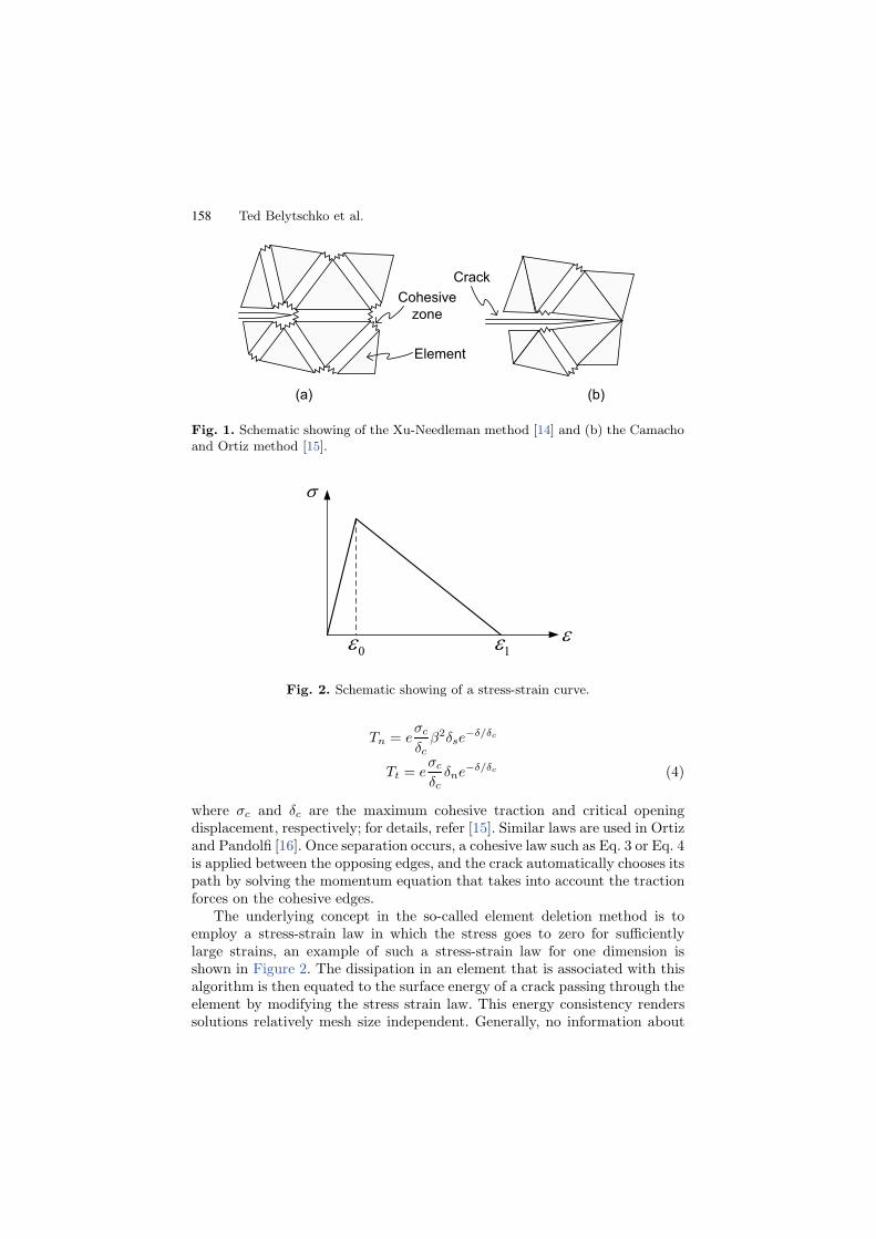
Fig. 1. Schematic showing of the Xu-Needleman method [14] and (b) the Camachoand Ortiz method [15].

V

H0H

1H

Fig. 2. Schematic showing of a stress-strain curve.

Tn = eσc

δcβ2δse

−δ/δc

Tt = eσc

δcδne−δ/δc (4)

where σc and δc are the maximum cohesive traction and critical openingdisplacement, respectively; for details, refer [15]. Similar laws are used in Ortizand Pandolfi [16]. Once separation occurs, a cohesive law such as Eq. 3 or Eq. 4is applied between the opposing edges, and the crack automatically chooses itspath by solving the momentum equation that takes into account the tractionforces on the cohesive edges.

The underlying concept in the so-called element deletion method is toemploy a stress-strain law in which the stress goes to zero for sufficientlylarge strains, an example of such a stress-strain law for one dimension isshown in Figure 2. The dissipation in an element that is associated with thisalgorithm is then equated to the surface energy of a crack passing through theelement by modifying the stress strain law. This energy consistency renderssolutions relatively mesh size independent. Generally, no information about

158


the orientation of the crack surface is included, so it is best to use square ornearly square elements.

To illustrate the energy equivalence in two dimensional problems for thestress-strain law shown in Figure 2, the upper strain limit ϵ1 is scaled so that

Gfhe =12Eϵ0 ϵ1A

e (5)

where Gf is the fracture energy, he is a characteristic dimension (the length ofa side for a square element), and Ae is the area of the element, unit thickness isassumed. While the method is called an element deletion method, the elementis not deleted, but instead the stress in the element is set to zero. Someprograms, such as LS-DYNA [17], remove the mass of the element from theglobal mass matrix to eliminate the inertia effects for these elements, but thisseems unwarranted, since the mass does not disappear. We have retained themass, but for the problems considered here, it makes little difference.

In the calculations reported here, we used the continuum damage modelproposed by Lemaitre [18]. The damage evolution law is given by

D(ϵ) = 1 − (1 − A)ϵ0 ϵ−1 − Ae−B⟨ϵ−ϵ0⟩ (6)

where D is the damage parameter which can have values 0 to 1, ϵ is theeffective strain, A and B are material parameters, ϵ0 is the strain threshold,and ⟨·⟩ is the MacCaulay bracket. The constitutive relation is given by:

σij = (1 − D)Cijklϵkl (7)

where Cijkl is the elastic modulus of the undamaged material, and σij andϵkl are stress and strain components, respectively.

All calculations were performed with 3 node triangular elements or 4 nodequadrilateral elements in which one point integration rule is used. Both struc-tured and unstructured meshes were used as noted; all calculations were madewith explicit time integration. The time step was usually a very small fractionof the stable time step. This appears to be unavoidable in crack propagationproblems at this time.

2 Benchmark Problem

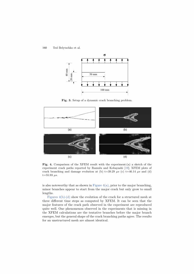
We have chosen as a benchmark problem crack growth in a prenotched glasssheet. The setup of the problem is shown in Figure 3. As can be seen, a tensilestress σy = 1 MPa is applied at the top and bottom surfaces; the time historyof the load is a step function. Experiment on specimens of similar dimensionshave been reported by [19–23].

In these experiments, a crack starts growing at the notch and propagatesto the right, generally with increasing speed. At a certain point, the crackbranches into at least two cracks (some experiments show more branches). It

159


100 mm

40

mm

50 mm

20

mm

ı

Fig. 3. Setup of a dynamic crack branching problem.

(a) (b)

(c) (d)

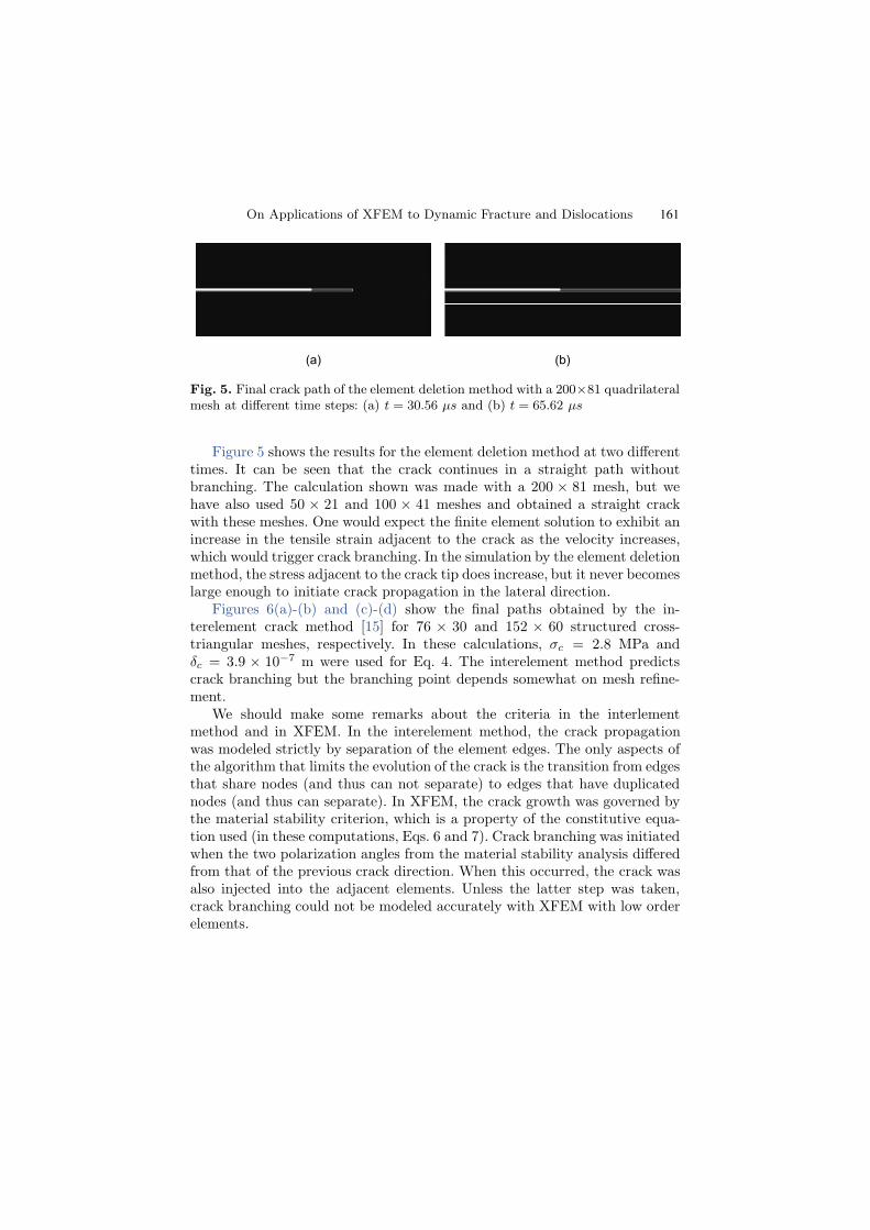
Fig. 4. Comparison of the XFEM result with the experiment:(a) a sketch of theexperiment crack paths reported by Ramulu and Kobayashi [19]; XFEM plots ofcrack branching and damage evolution at (b) t=39.29 µs (c) t=46.14 µs and (d)t=55.93 µs.

is also noteworthy that as shown in Figure 4(a), prior to the major branching,minor branches appear to start from the major crack but only grow to smalllengths.

Figures 4(b)-(d) show the evolution of the crack for a structured mesh atthree different time steps as computed by XFEM. It can be seen that themajor features of the crack path observed in the experiment are reproducedquite well. One phenomenon observed in the experiments that is missing inthe XFEM calculations are the tentative branches before the major branchemerges, but the general shape of the crack branching paths agree. The resultsfor an unstructured mesh are almost identical.

160


(a) (b)

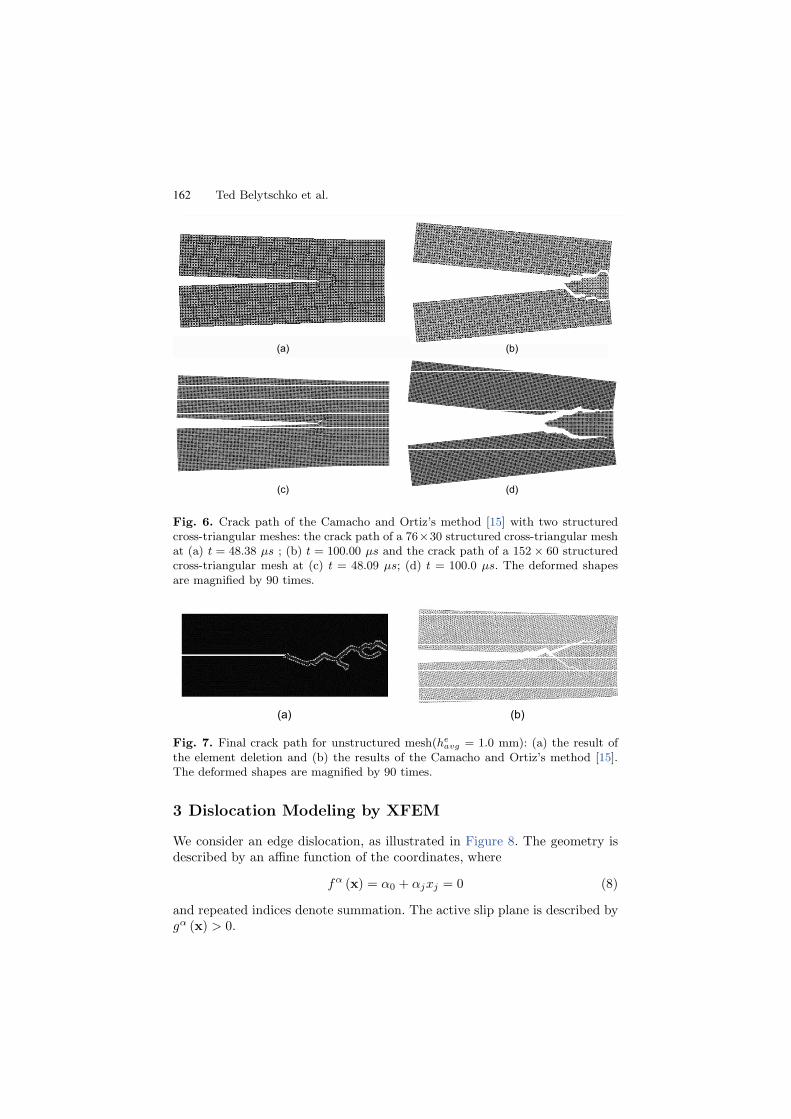
Fig. 5. Final crack path of the element deletion method with a 200×81 quadrilateralmesh at different time steps: (a) t = 30.56 µs and (b) t = 65.62 µs

Figure 5 shows the results for the element deletion method at two differenttimes. It can be seen that the crack continues in a straight path withoutbranching. The calculation shown was made with a 200 × 81 mesh, but wehave also used 50 × 21 and 100 × 41 meshes and obtained a straight crackwith these meshes. One would expect the finite element solution to exhibit anincrease in the tensile strain adjacent to the crack as the velocity increases,which would trigger crack branching. In the simulation by the element deletionmethod, the stress adjacent to the crack tip does increase, but it never becomeslarge enough to initiate crack propagation in the lateral direction.

Figures 6(a)-(b) and (c)-(d) show the final paths obtained by the in-terelement crack method [15] for 76 × 30 and 152 × 60 structured cross-triangular meshes, respectively. In these calculations, σc = 2.8 MPa andδc = 3.9 × 10−7 m were used for Eq. 4. The interelement method predictscrack branching but the branching point depends somewhat on mesh refine-ment.

We should make some remarks about the criteria in the interlementmethod and in XFEM. In the interelement method, the crack propagationwas modeled strictly by separation of the element edges. The only aspects ofthe algorithm that limits the evolution of the crack is the transition from edgesthat share nodes (and thus can not separate) to edges that have duplicatednodes (and thus can separate). In XFEM, the crack growth was governed bythe material stability criterion, which is a property of the constitutive equa-tion used (in these computations, Eqs. 6 and 7). Crack branching was initiatedwhen the two polarization angles from the material stability analysis differedfrom that of the previous crack direction. When this occurred, the crack wasalso injected into the adjacent elements. Unless the latter step was taken,crack branching could not be modeled accurately with XFEM with low orderelements.

161


(a) (b)

(c) (d)

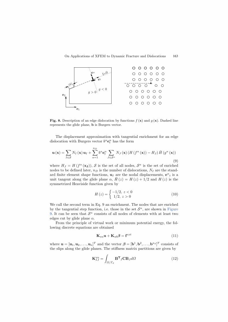
Fig. 6. Crack path of the Camacho and Ortiz’s method [15] with two structuredcross-triangular meshes: the crack path of a 76×30 structured cross-triangular meshat (a) t = 48.38 µs ; (b) t = 100.00 µs and the crack path of a 152 × 60 structuredcross-triangular mesh at (c) t = 48.09 µs; (d) t = 100.0 µs. The deformed shapesare magnified by 90 times.

(a) (b)

Fig. 7. Final crack path for unstructured mesh(heavg = 1.0 mm): (a) the result of

the element deletion and (b) the results of the Camacho and Ortiz’s method [15].The deformed shapes are magnified by 90 times.

3 Dislocation Modeling by XFEM

We consider an edge dislocation, as illustrated in Figure 8. The geometry isdescribed by an affine function of the coordinates, where

fα (x) = α0 + αjxj = 0 (8)

and repeated indices denote summation. The active slip plane is described bygα (x) > 0.

162


e t

e2

e1

en

||b||

f=0

g > 0g < 0

Fig. 8. Description of an edge dislocation by functions f (x) and g (x). Dashed linerepresents the glide plane, b is Burgers vector.

The displacement approximation with tangential enrichment for an edgedislocation with Burgers vector bαeα

t has the form

u (x) =∑

I∈SNI (x)uI +

nD∑

α=1

bαeαt

∑

J∈Sα

NJ (x) (H (fα (x)) − HJ) H (gα (x))

(9)where HJ = H (fα (xJ)), S is the set of all nodes, Sα is the set of enrichednodes to be defined later, nD is the number of dislocations, NI are the stand-ard finite element shape functions, uI are the nodal displacements, eα

t is aunit tangent along the glide plane α, H (z) = H (z) + 1/2 and H (z) is thesymmetrized Heaviside function given by

H (z) =−1/2, z < 01/2, z > 0 (10)

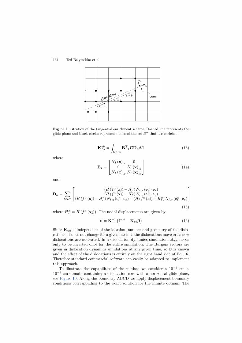
We call the second term in Eq. 9 an enrichment. The nodes that are enrichedby the tangential step function, i.e. those in the set Sα, are shown in Figure9. It can be seen that Sα consists of all nodes of elements with at least twoedges cut by glide plane α.

From the principle of virtual work or minimum potential energy, the fol-lowing discrete equations are obtained

Kuuu + Kubβ = fext (11)

where u = [u1,u2, . . . ,un]T and the vector β = [b1,b2, . . . ,bnd ]T consists ofthe slips along the glide planes. The stiffness matrix partitions are given by

KuuIJ =

∫

Ω/Γd

BTICBJdΩ (12)

163


et

glideplan

ecore

en

ut = b

ut = b

ut = b

Fig. 9. Illustration of the tangential enrichment scheme. Dashed line represents theglide plane and black circles represent nodes of the set Sα that are enriched.

KubIα =

∫

Ω/Γd

BTICDαdΩ (13)

where

BI =

⎡

⎣NI (x),x 0

0 NI (x),y

NI (x),y NI (x),x

⎤

⎦ (14)

and

Dα =∑

I∈Sα

⎡

⎣(H (fα (x)) − Hα

I )NI,x (eαt · ex)

(H (fα (x)) − HαI )NI,y (eα

t · ey)(H (fα (x)) − Hα

I )NI,y (eαt · ex) + (H (fα (x)) − Hα

I )NI,x (eαt · ey)

⎤

⎦

(15)where Hα

I = H (fα (xI)). The nodal displacements are given by

u = K−1uu

(fext − Kubβ

)(16)

Since Kuu is independent of the location, number and geometry of the dislo-cations, it does not change for a given mesh as the dislocations move or as newdislocations are nucleated. In a dislocation dynamics simulation, Kuu needsonly to be inverted once for the entire simulation. The Burgers vectors aregiven in dislocation dynamics simulations at any given time, so β is knownand the effect of the dislocations is entirely on the right hand side of Eq. 16.Therefore standard commercial software can easily be adapted to implementthis approach.

To illustrate the capabilities of the method we consider a 10−4 cm ×10−4 cm domain containing a dislocation core with a horizontal glide plane,see Figure 10. Along the boundary ABCD we apply displacement boundaryconditions corresponding to the exact solution for the infinite domain. The

164


A B

D C

A

D C

B

x

y x’

y’b

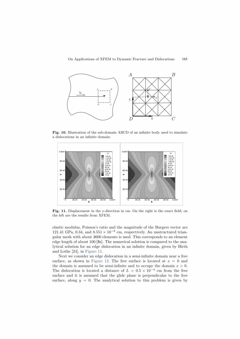
Fig. 10. Illustration of the sub-domain ABCD of an infinite body used to simulatea dislocations in an infinite domain.

X

Y

0 2E-05 4E-05 6E-05 8E-05 0.00010

2E-05

4E-05

6E-05

8E-05

0.0001UY

1.2E-081.15E-081.1E-081.05E-081E-089.5E-099E-098.5E-098E-097.5E-097E-09

X

Y

0 2E-05 4E-05 6E-05 8E-05 0.00010

2E-05

4E-05

6E-05

8E-05

0.0001UY

1.2E-081.15E-081.1E-081.05E-081E-089.5E-099E-098.5E-098E-097.5E-097E-09

Fig. 11. Displacement in the y-direction in cm. On the right is the exact field; onthe left are the results from XFEM.

elastic modulus, Poisson’s ratio and the magnitude of the Burgers vector are121.41 GPa, 0.34, and 8.551 × 10−8 cm, respectively. An unstructured trian-gular mesh with about 3600 elements is used. This corresponds to an elementedge length of about 100 ∥b∥. The numerical solution is compared to the ana-lytical solution for an edge dislocation in an infinite domain, given by Hirthand Lothe [24], in Figure 11.

Next we consider an edge dislocation in a semi-infinite domain near a freesurface, as shown in Figure 12. The free surface is located at x = 0 andthe domain is assumed to be semi-infinite and to occupy the domain x > 0.The dislocation is located a distance of L = 0.5 × 10−4 cm from the freesurface and it is assumed that the glide plane is perpendicular to the freesurface, along y = 0. The analytical solution to this problem is given by

165


A B

CDFREE

SU

RFA

CE

x

y

L

10−2

10−1

10−2

10−1

100

1/he 10−4 cm

rela

tive

ener

gy e

rror

nor

m

1.0

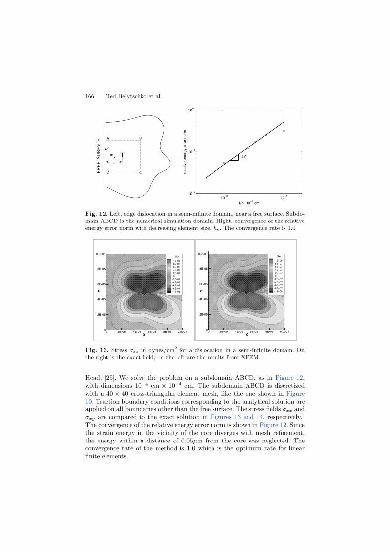
Fig. 12. Left, edge dislocation in a semi-infinite domain, near a free surface. Subdo-main ABCD is the numerical simulation domain. Right, convergence of the relativeenergy error norm with decreasing element size, he. The convergence rate is 1.0

X

Y

0 2E-05 4E-05 6E-05 8E-05 0.00010

2E-05

4E-05

6E-05

8E-05

0.0001Sxx

1E+088E+076E+074E+072E+070

-2E+07-4E+07-6E+07-8E+07-1E+08

X

Y

0 2E-05 4E-05 6E-05 8E-05 0.00010

2E-05

4E-05

6E-05

8E-05

0.0001Sxx

1E+088E+076E+074E+072E+070

-2E+07-4E+07-6E+07-8E+07-1E+08

Fig. 13. Stress σxx in dynes/cm2 for a dislocation in a semi-infinite domain. Onthe right is the exact field; on the left are the results from XFEM.

Head, [25]. We solve the problem on a subdomain ABCD, as in Figure 12,with dimensions 10−4 cm × 10−4 cm. The subdomain ABCD is discretizedwith a 40 × 40 cross-triangular element mesh, like the one shown in Figure10. Traction boundary conditions corresponding to the analytical solution areapplied on all boundaries other than the free surface. The stress fields σxx andσxy are compared to the exact solution in Figures 13 and 14, respectively.The convergence of the relative energy error norm is shown in Figure 12. Sincethe strain energy in the vicinity of the core diverges with mesh refinement,the energy within a distance of 0.05µm from the core was neglected. Theconvergence rate of the method is 1.0 which is the optimum rate for linearfinite elements.

166


X

Y

0 2E-05 4E-05 6E-05 8E-05 0.00010

2E-05

4E-05

6E-05

8E-05

0.0001Sxy

1E+088E+076E+074E+072E+070

-2E+07-4E+07-6E+07-8E+07-1E+08

XY

0 2E-05 4E-05 6E-05 8E-05 0.00010

2E-05

4E-05

6E-05

8E-05

0.0001Sxy

1E+088E+076E+074E+072E+070

-2E+07-4E+07-6E+07-8E+07-1E+08

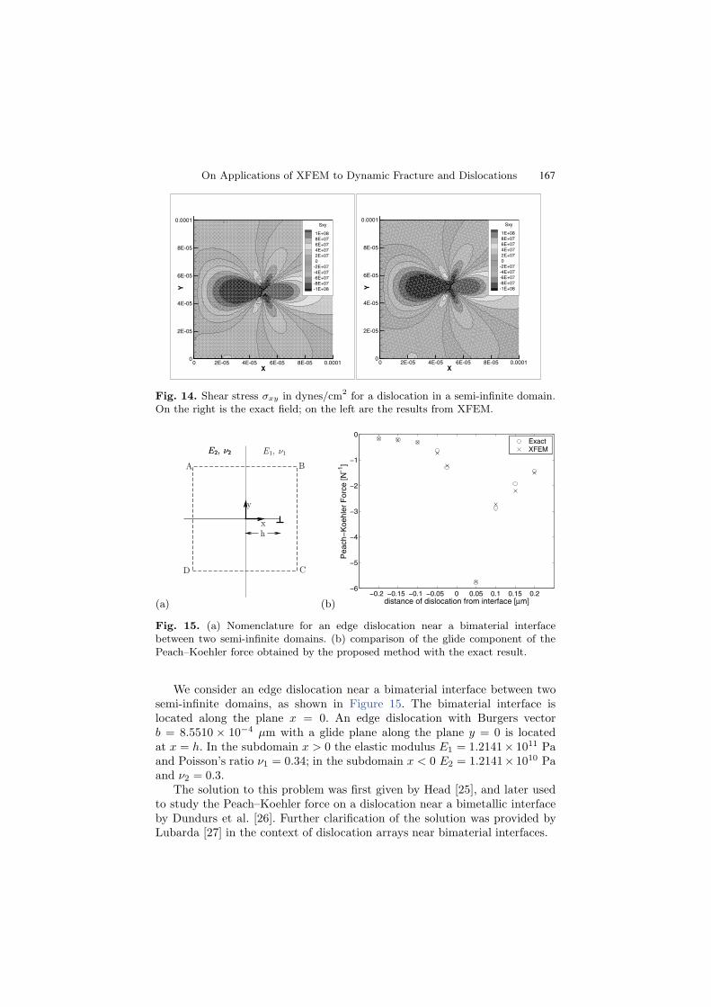
Fig. 14. Shear stress σxy in dynes/cm2 for a dislocation in a semi-infinite domain.On the right is the exact field; on the left are the results from XFEM.

(a)

h

E1, ν1E2, ν2

x

y

A

E2, ν2

B

CD

(b)−0.2 −0.15 −0.1 −0.05 0 0.05 0.1 0.15 0.2

−6

−5

−4

−3

−2

−1

0

Pea

ch−K

oehl

er F

orce

[N−1

]

distance of dislocation from interface [µm]

ExactXFEM

Fig. 15. (a) Nomenclature for an edge dislocation near a bimaterial interfacebetween two semi-infinite domains. (b) comparison of the glide component of thePeach–Koehler force obtained by the proposed method with the exact result.

We consider an edge dislocation near a bimaterial interface between twosemi-infinite domains, as shown in Figure 15. The bimaterial interface islocated along the plane x = 0. An edge dislocation with Burgers vectorb = 8.5510 × 10−4 µm with a glide plane along the plane y = 0 is locatedat x = h. In the subdomain x > 0 the elastic modulus E1 = 1.2141 × 1011 Paand Poisson’s ratio ν1 = 0.34; in the subdomain x < 0 E2 = 1.2141 × 1010 Paand ν2 = 0.3.

The solution to this problem was first given by Head [25], and later usedto study the Peach–Koehler force on a dislocation near a bimetallic interfaceby Dundurs et al. [26]. Further clarification of the solution was provided byLubarda [27] in the context of dislocation arrays near bimaterial interfaces.

167


X

Y

0 2E-05 4E-05 6E-05 8E-05 0.00010

2E-05

4E-05

6E-05

8E-05 Sxy

5E+074E+073E+072E+071E+070

-1E+07-2E+07-3E+07-4E+07-5E+07

XY

2E-05 4E-05 6E-05 8E-05 0.00010

2E-05

4E-05

6E-05

8E-05 Sxy

5E+074E+073E+072E+071E+070

-1E+07-2E+07-3E+07-4E+07-5E+07

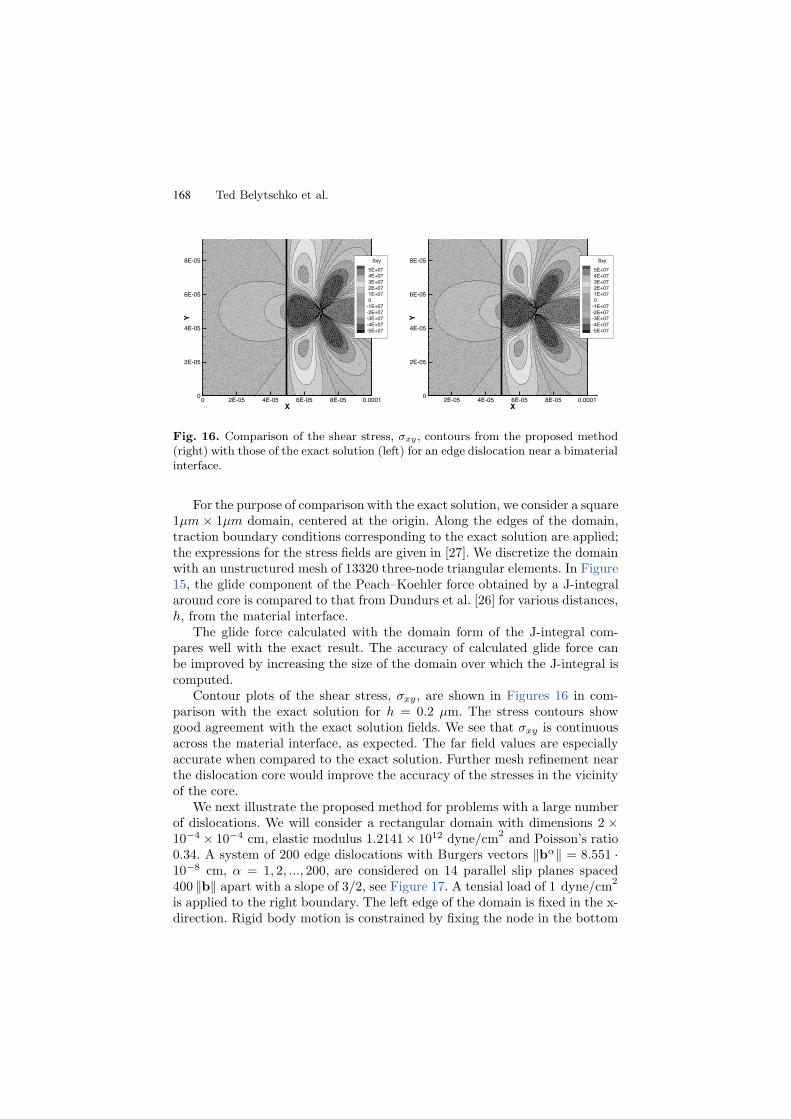
Fig. 16. Comparison of the shear stress, σxy , contours from the proposed method(right) with those of the exact solution (left) for an edge dislocation near a bimaterialinterface.

For the purpose of comparison with the exact solution, we consider a square1µm × 1µm domain, centered at the origin. Along the edges of the domain,traction boundary conditions corresponding to the exact solution are applied;the expressions for the stress fields are given in [27]. We discretize the domainwith an unstructured mesh of 13320 three-node triangular elements. In Figure15, the glide component of the Peach–Koehler force obtained by a J-integralaround core is compared to that from Dundurs et al. [26] for various distances,h, from the material interface.

The glide force calculated with the domain form of the J-integral com-pares well with the exact result. The accuracy of calculated glide force canbe improved by increasing the size of the domain over which the J-integral iscomputed.

Contour plots of the shear stress, σxy, are shown in Figures 16 in com-parison with the exact solution for h = 0.2 µm. The stress contours showgood agreement with the exact solution fields. We see that σxy is continuousacross the material interface, as expected. The far field values are especiallyaccurate when compared to the exact solution. Further mesh refinement nearthe dislocation core would improve the accuracy of the stresses in the vicinityof the core.

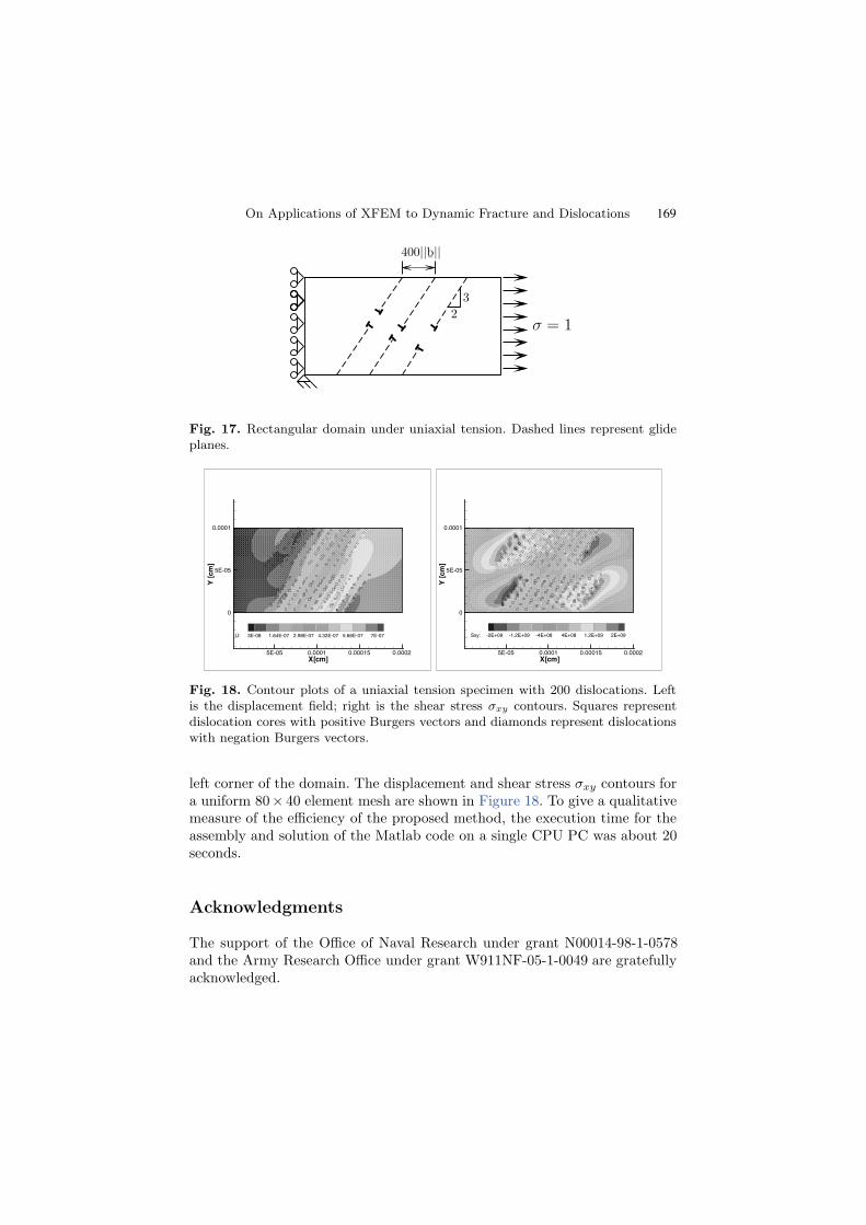
We next illustrate the proposed method for problems with a large numberof dislocations. We will consider a rectangular domain with dimensions 2 ×10−4 × 10−4 cm, elastic modulus 1.2141 × 1012 dyne/cm2 and Poisson’s ratio0.34. A system of 200 edge dislocations with Burgers vectors ∥bα∥ = 8.551 ·10−8 cm, α = 1, 2, ..., 200, are considered on 14 parallel slip planes spaced400 ∥b∥ apart with a slope of 3/2, see Figure 17. A tensial load of 1 dyne/cm2

is applied to the right boundary. The left edge of the domain is fixed in the x-direction. Rigid body motion is constrained by fixing the node in the bottom

168


σ = 1

400||b¯||

23

Fig. 17. Rectangular domain under uniaxial tension. Dashed lines represent glideplanes.

X[cm]

Y[c

m]

5E-05 0.0001 0.00015 0.0002

0

5E-05

0.0001

U: 3E-08 1.64E-07 2.98E-07 4.32E-07 5.66E-07 7E-07

X[cm]

Y[c

m]

5E-05 0.0001 0.00015 0.0002

0

5E-05

0.0001

Sxy: -2E+09 -1.2E+09 -4E+08 4E+08 1.2E+09 2E+09

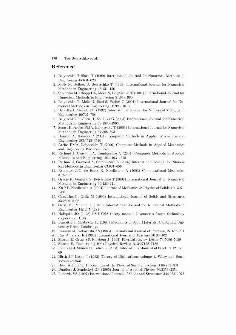
Fig. 18. Contour plots of a uniaxial tension specimen with 200 dislocations. Leftis the displacement field; right is the shear stress σxy contours. Squares representdislocation cores with positive Burgers vectors and diamonds represent dislocationswith negation Burgers vectors.

left corner of the domain. The displacement and shear stress σxy contours fora uniform 80 × 40 element mesh are shown in Figure 18. To give a qualitativemeasure of the efficiency of the proposed method, the execution time for theassembly and solution of the Matlab code on a single CPU PC was about 20seconds.

Acknowledgments

The support of the Office of Naval Research under grant N00014-98-1-0578and the Army Research Office under grant W911NF-05-1-0049 are gratefullyacknowledged.

169


References

1. Belytschko T,Black T (1999) International Journal for Numerical Methods inEngineering 45:601–620

2. Moes N, Dolbow J, Belytschko T (1999) International Journal for NumericalMethods in Engineering 46:131–150

3. Stolarska M, Chopp DL, Moes N, Belytschko T (2001) International Journal forNumerical Methods in Engineering 51:943–960

4. Belytschko T, Moes N, Usui S, Parimi C (2001) International Journal for Nu-merical Methods in Engineering 50:993–1013

5. Babuska I, Melenk JM (1997) International Journal for Numerical Methods inEngineering 40:727–758

6. Belytschko T, Chen H, Xu J, Zi G (2003) International Journal for NumericalMethods in Engineering 58:1873–1905

7. Song JH, Areias PMA, Belytschko T (2006) International Journal for NumericalMethods in Engineering 67:868–893

8. Hansbo A, Hansbo P (2004) Computer Methods in Applied Mechanics andEngineering 193:3523–3540

9. Areias PMA, Belytschko T (2006) Computer Methods in Applied Mechanicsand Engineering 195:1275–1276

10. Rethore J, Gravouil A, Combescure A (2004) Computer Methods in AppliedMechanics and Engineering 193:4493–4510

11. Rethore J, Gravouil A, Combescure A (2005) International Journal for Numer-ical Methods in Engineering 63:631–659

12. Remmers JJC, de Borst R, Needleman A (2003) Computational Mechanics31:69–77

13. Gracie R, Ventura G, Belytschko T (2007) International Journal for NumericalMethods in Engineering 69:423–441

14. Xu XP, Needleman A (1994) Journal of Mechanics & Physics of Solids 42:1397–1434

15. Camacho G, Ortiz M (1996) International Journal of Solids and Structures33:2899–2938

16. Ortiz M, Pandolfi A (1999) International Journal for Numerical Methods inEngineering 44:1267–1282

17. Hallquist JO (1998) LS-DYNA theory manual. Livemore software thchnologycorporation, USA

18. Lemaitre J, Chaboche JL (1990) Mechanics of Solid Materials. Cambridge Uni-versity Press, Cambridge

19. Ramulu M, Kobayashi AS (1985) International Journal of Fracture, 27:187–20120. Ravi-Chandar K (1998) International Journal of Fracture 90:83–10221. Sharon E, Gross SP, Fineberg J (1995) Physical Review Letter 74:5096–509922. Sharon E, Fineberg J (1996) Physical Review B, 54:7128–713923. Fineberg J, Sharon E, Cohen G (2003) International Journal of Fracture 121:55–

6924. Hirth JP, Lothe J (1982) Theory of Dislocations: volume 1. Wiley and Sons,

second edition25. Head AK (1953) Proceedings of the Physical Society. Section B 66:793–80126. Dundurs J, Sendeckyj GP (1965) Journal of Applied Physics 36:3353–335427. Lubarda VA (1997) International Journal of Solids and Structures 34:1053–1073

170

on applications of xfem to dynamic fracture and dislocations

Documents