on a double-threshold autoregressive heteroscedastic time series model
TRANSCRIPT
JOURNAL OF APPLIED ECONOMETRICS, VOL. 11,253-274 (1996)
ON A DOUBLE-THRESHOLD AUTOREGRESSIVE HETEROSCEDASTIC TIME SERIES MODEL
C. W. LI AND W. K. LI Department of Statistics, University of Hong Kong, Pokfulanr Road, Hong Kong
SUMMARY
Tong’s threshold models have been found useful in modelling nonlinearities in the conditional mean of a time series. The threshold model is extended to the so-called double-threshold ARCH(DTARCH) model, which can handle the situation where both the conditional mean and the conditional variance specifications are piecewise linear given previous information. Potential applications of such models include financial data with different (asymmetric) behaviour in a rising versus a falling market and business cycle modelling. Model identification, estimation and diagnostic checking techniques are developed. Maximum likelihood estimation can be achieved via an easy-to-use iteratively weighted least squares algorithm. Portmanteau-type statistics are also derived for checking model adequacy. An illustrative example demonstrates that asymmetric behaviour in the mean and the variance could be present in financial series and that the DTARCH model is capable of capturing these phenomena.
1. INTRODUCTION
The concept of ARCH, which stands for Autoregressive Conditional Heteroscedasticity , was first introduced by Engle (1982) to handle time series with a changing conditional variance. It was then shown to be a useful model in financial applications (Christie, 1982; Engle and Bollerslev, 1986; Hinich and Patterson, 1985; French, Schwert and Stambaugh, 1987; Schwert, 1989; Nelson, 1991). Bollerslev (1986) extended the ARCH model into the so-called Generalized Autoregressive Conditional Heteroscedastic model (GARCH). On the other hand, time series analysis has gone well beyond the linear models of Box and Jenkins and a popular class of nonlinear time series model is the threshold models of Tong (1978) and Tong and Lim (1980). Tong (1990, p. 116) suggested a threshold model with a changing conditional variance, which is entitled the SETAR-ARCH model. This model has a piecewise linear conditional mean and an ARCH innovation. It combines the advantages of the SETAR model and the ARCH model.
Although the SETAR-ARCH model may have many applications (Li and Lam, 1995), it has assumed a fixed description of the conditional variance. Several authors have pointed out that in financial time series the behaviour of the conditional variance is probably asymmetric conditional on previous returns (Rabemanjara and Zakoian, 1993; Campbell and Hentschell, 1990; Christie, 1982; Nelson, 1990, 1991; Schwert, 1989). For example, Schwert (1989) found that financial assets’ volatility is usually high during recessions. On the other hand, there is a Wall Street ‘adage’ that volume is relatively heavy in bull markets and light in bear markets. Such asymmetry in a price-volume relationship is well known (Karpoff, 1987). This suggests
CCC 0883-7252/96/030253-22 0 1996 by John Wiley & Sons, Ltd.
Received 30 August I994 Revised November 1995
254 C. W. LI AND W. K. LI
that asymmetric volatility could be a characteristic of financial time series. In order to deal with such situations, a double-threshold autoregressive conditional heteroscedastic time series (DTARCH) model is proposed. Hamilton (1990) considered a special case of the general SETAR class model in which an appropriate indicator time series is invoked. However, this takes the form of a latent driving force process behind such changes, and is different from the model we are going to discuss. The DTARCH model does not assume such an unobserved process and thus is expected to be much easier to understand and estimate.
One advantage of the SETAR-type models is that they can model limit cycle behaviour in a natural way. For example, in their study of the business cycles of 13 OECD countries Terasvirta and Anderson (1993) used a smoothed transition SETAR model. However, these models assume a homoscedastic variance for the distribution of the white-noise disturbance. As will be shown in this paper, this assumption may not be adequate in financial time series. Beaudry and Koop (1993) proposed a business cycle model where the growth rate of the economy depends on a variable that indicates the depth of recession. In a more recent work on business cycle modelling Pesaran and Potter (1994) proposed a model that incorporates indicators for both the depth of recession and overheating during economic expansion. They called this type of model 'floor and ceiling' model. All these models have the flavour of a general threshold model in the sense that a different model structure will be in effect if a certain threshold is triggered. However, a significant new element in Pesaran and Potter (1994) is that the variance of the disturbance is also allowed to be dependent on the current state of the economy, the states (regimes) being determined by past observations and the threshold structures. This development is clearly important in view of the observation by Schwert (1 989) on the apparent relationship between volatility and business cycle. The DTARCH model proposed in this paper is closely related to this development in business cycle modelling. With suitable modifications the results here can be applied to the 'floor and ceiling' types of business cycle model.
In this paper the DTARCH model is proposed to allow for a different ARCH specification conditional on previous information. Model identification, parameter estimation and a model diagnostic method for the DTARCH models are developed. Model identification includes estimating the delay parameter, threshold parameter, AR orders and ARCH orders. This can be achieved by extending the arranged autoregression technique in Tsay (1989). An iteratively weighted least square (IWLS) approach (Mak and Li, 1994) is introduced for maximum likelihood estimation. Model diagnostics are introduced by using standardized residual autocorrelations and squared residual autocorrelations. Asymptotic distributions of residual autocorrelations and squared residual autocorrelations are derived in the same way as Li (1992) and Li and Mak (1994). The asymptotic covariance matrices provide the correct large sample standard errors for these quantities and portmanteau type tests Q,n(M) and Q,,,,,(M) are introduced for the overall diagnosis of the conditional mean and conditional variance specifications. The relative merits of these statistics in model construction were studied using simulation. Consistency and asymptotic normality of maximum likelihood estimates are also discussed.
The paper is organized as follows. In Section 2, definition and assumptions of the DTARCH model will be given. Section 3 deals with the identification of a DTARCH model. Section 4 discusses the MLE of a DTARCH model and presents an IWLS approach for maximum likelihood estimation. Comparison of computational efficiency will be made with the Quasi- Newton method. Section 5 presents the asymptotic normality of residual autocorrelations and square residual autocorrelations, and chi-square statistics Q,, , (M) and Q,",,,(M) are then introduced for the overall diagnosis of the conditional mean and conditional variance. In Section
A DOUBLE-THRESHOLD AUTOREGRESSIVE TIME SERIES MODEL 255
6, a DTARCH model is applied to the Daily Hong Kong Hang Seng Index return from 1982 to 1991. Discussion will be given in Section 7.
2. DEFINITION OF THE DTARCH MODEL AND ASSUMPTIONS
Let Y,-l be the a-field generated by the random variables [ u1-; I i = 1, 2, ...). For each t , given information a, is a normally distributed random variable, with mean zero and conditional variance, E(a: I TI-,) = h,, where E ( - 1 Y,-,) denotes conditional expectation given A time series { X I ) is a Double-Threshold Autoregressive Conditional Heteroscedastic process, if it follows the model,
r = 1
where j = 1, 2, ..., rn and d is the delay parameter. The threshold parameters rI satisfy -= = rn < rl < r2 ... < rm = 00. Note that it is straightforward to allow for different delays and different sets of threshold parameters for the mean and variance. Further, the threshold effect might not be present in both the mean and the variance.
The DTARCH model extends Tong's threshold model in a natural way. Tong and Lim (1 980) showed that the threshold model is capable of capturing various nonlinear phenomena, such as asymmetric cycles, jump resonance and amplitude-frequency dependence. The special conditional mean structure of DTARCH model is similar to the threshold model, therefore it has the same threshold nonlinear characteristics as that of the threshold model. We denote model (1) as DTARCH(pI, p 2 ..., p,,,; q l , q2, ..., 4,"). The first rn integers, p i , p2, ..., p , , represent the AR orders in the m regimes, while the last rn integers, q l , q2, ..., qm, represent the corresponding ARCH orders. If the ARCH order within a regime is zero, then the conditional variance of this regime is constant. Clearly, if other variables such as hl-d or are used in the place of XI+ the results of this paper can be adapted to these cases with suitable modifications.
For the sake of further development, the assumptions in Weiss (1986) on ARCH model are employed and they are summarized in the following six regular conditions:
(1) The time series { X I ) is stationary and ergodic. (2) E(X,?) < and (3) All the parameters in the conditional variance are positive or non-negative, aL">O and
a! ' "zOforr=l ,2 ,..., q l a n d j = 1 , 2 ,..,, m. (4) (1, a:-,, ..., a;-[,A) is linearly independent for k = 1, 2, ..., m, i.e. for any /lo, PI , ... B,;
i fBo+Bia : - , + . . . + B 9ku:- qk=OthenBn=B,=. . .=B, ,=O ( 5 ) Model (1) is stationary when h, is constant within each regime. (6) Let a(')= (a;'), a;'), ...,
2
( I ) ) then a ( I ) + a (") if k # k' and a similar condition holds for
Conditions (1), ( 2 ) , (3) and ( 5 ) are the usual assumptions on a stationary conditional heteroscedastic and threshold nonlinear time series process (Tong, 1990). Condition (4) ensures the identification of the parameters a(') (Weiss, 1986). Condition (6) is required for the full DTARCH model to be identifiable. In the following sections we will concentrate our discussion
( 1 ) - @(I' @ ( I ) 0 ) 7- Q, - ( 0 t i ) .

256 C. W. LI AND W. K. LI
1 i = I
r ‘I I
1 I = 1
Similar results can be obtained for the general model DTARCH(p,, p 2 , ..., pm; q , , qr, ..., q,n) Note that if the conditional mean is simply an AR(p) model, we have a DTARCH(p; q , , q2 ) model, which is equivalent to an AR-TARCH(p; (I,, q2) model. The AR-TARCH process has a linear AR(p) conditional mean and a threshold nonlinear conditional variance. Similarly, if the conditional variance is a simple ARCH(q) model, we have a DTARCH(p,, p2; q ) model or, equivalently, a SETAR-ARCH(p, , p 2 ; q ) model. The original SETAR model will be denoted by SETAR(p,, p 2 ) . Finally, a DTARCH(p; q ) model is equivalent to an AR-ARCH(p; q ) model.
3. MODEL IDENTIFICATION
The Box and Jenkins time series modelling methodology consists of three steps: model identification, parameter estimation and diagnostic checking. Model identification will be presented now and parameter estimation and diagnostic checking will be discussed in the next two sections. For a linear AR model, model identification is done by examining the ACF and PACF of the process. However, when identifying a DTARCH model, this simple approach would not be effective apart from giving a rough upper bound of the AR orders. This is because autocorrelations are uninfoimative about asymmetries in the model. Tsay (1989) used arranged autoregression to model the threshold model. He proposed procedures for testing threshold nonlinearity and using various scatterplots to identify the threshold parameters. The AIC is then used to identify the AR orders of each regime.
We consider the AR-ARCH process first. An AR-ARCH(p; q ) process is a process X , given by X , = a0 + (PIX,-, + ... + QP,X,-, + a,, with conditional variance given by h,=a,+ a ,a f_ ,+ . . -+ a,&, .Let v ,=q2-h, .Thenwehave
(3)
The v, is a sequence of martingale differences, namely given 3,-], E(v , ( 3, - , )=0 and, furthermore, E ( V , U , - ~ ) = 0 for k > O . Therefore, the conditional variance can be rewritten in the form of a linear regression and Tsay’s arranged autoregression can be extended to the DTARCH models.
The preliminary identification procedure is divided into two parts; the first applies Tsay ’s procedure to identify the delay, threshold parameters and the AR orders in the conditional mean. If threshold structure is found the second part merely identifies the ARCH orders in the conditional variance using equation (3). For each regime, the squared residuals from the best
ar2 = a. + a,a,’_, + ... + a&-, + v,
A DOUBLE-THRESHOLD AUTOREGRESSIVE TIME SERIES MODEL 257
fitted SETAR model will replace in (3) . Otherwise, Tsay’s method based on (3) is applied to the squared residuals from the best-fitting AR model in identifying the threshold structure and the ARCH orders. If a threshold structure is identified a full DTARCH model will be considered. The second step extends Tsay ’s methodology to the conditional variance. A comprehensive review of the procedure for the conditional mean can be found in Tsay (1989) and the overall procedure is summarized as follows:
(1) Select the AR order p , the ARCH order q and the set S of possible delays. (2) Fit arranged autoregressions for a given p and each element d of S, and perform the
threshold nonlinear test F ( p , d). If nonlinearity of the process is detected, select the delay parameter d by the one maximizing F ( p , d).
(3) For given p and d, locate the threshold parameter by using Tsay’s arranged autoregression and the scatterplots of predictive residuals and t-ratios.
(4) If threshold structure is identified, calculate the residuals Ci, of the threshold AR model and identify the ARCH order using equation (3) and S,?.
(5) Otherwise, locate the threshold structure by applying arranged autoregression to equation (3) and the scatterplots of predictive residuals and t-ratios (the squared residuals from the best AR model replacing u: in equation (3)).
(6) Fit the entire DTARCH model by MLE if a threshold structure is identified. Otherwise just fit an AR-ARCH model.
(7) Use AIC to refine the AR orders, ARCH orders, the delay and threshold parameters by repeating steps (1)- (6) , if necessary.
In step (1) the maximum AR order p and ARCH order q may be selected by examining the ACF, PACF and the ACF of the squared series. The set of threshold lags S may be { 1, 2, ..., max(p, q ) ] . In step (2) there is the question of robustness of the F-statistic under a changing ARCH condition. Some simulation results were performed to investigate the power and size of the F-statistic under the DTARCH model. The results suggest that the power is as high as 0.8 for a sample size of 200 while the sizes are just slightly more sensitive. This seems to justify the use of the F-statistic here as a preliminary identification tool for the mean. Note that in steps (3) and ( 5 ) t-ratio scatterplots of AR and ARCH coefficients can be examined to locate the threshold parameters. Step (7) involves the refinement of the model that may rely on the Akalke Information Criterion (AIC) and other model-checking techniques. Chan (1993) suggested that d,, (the estimate of d ) in the SETAR model is strongly consistent. It is plausible that his result also holds here.
4. MAXIMUM LIKELIHOOD ESTIMATION BY IWLS
Given the specification of the model and assuming conditional Gaussianity, maximum likelihood estimation (MLE) can be performed. Asymptotic results for the MLE in Weiss (1986) can be extended easily to the DTARCH model, with a known threshold parameter r and known delay parameter d. We assume that these quantities are known because the derivation is much easier and in some applications, such as financial series, non-zero thresholds do not appear to be physically meaningful. If the parameters are unknown, the estimation of the delay parameter d does not provide a serious problem. Since there is only a finite number of choices for these estimates, the best one can be chosen by AIC. Chan (1993) showed that such an estimate of the delay parameter in the case of the SETAR model is strongly consistent. However, for the DTARCH model with a non-trivial ARCH component the problem become much more complicated. The non-differentiablity of the likelihood function prevents the usage
258 C. W. LI AND W. K. LI
of standard asymptotic results. Chan (1993) considered this problem for the threshold models. The proof for the unknown threshold and delay case can follow the argument of Chan, but it will not be considered here. A referee has pointed out that with a least squares loss function Chan's results should apply to the conditional mean estimates almost directly and so it seems plausible that the maximum likelihood estimates using the full model structure will also satisfy similar properties.
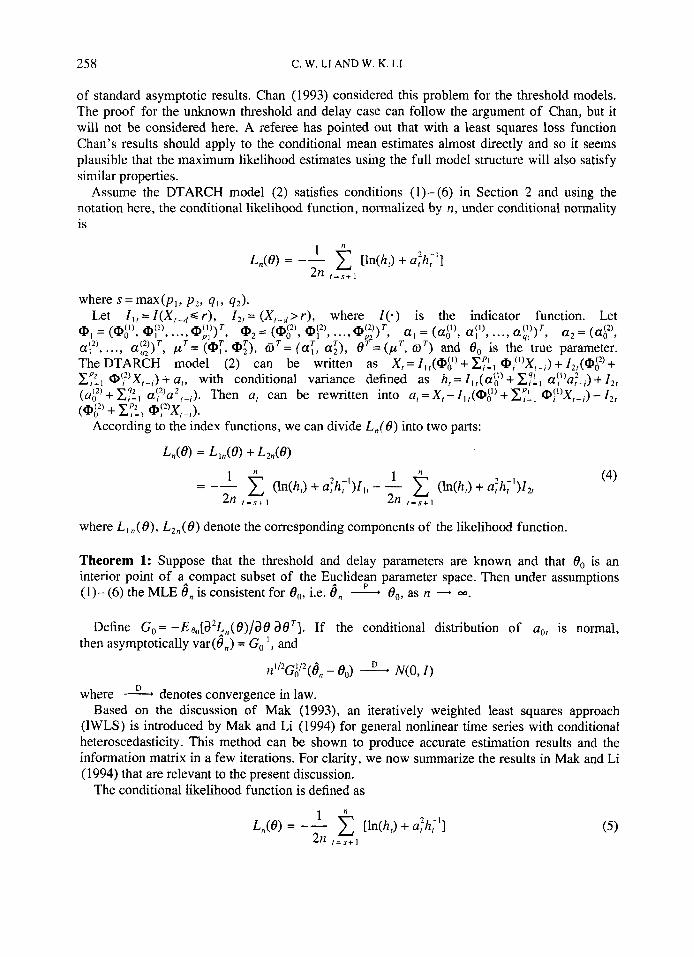
Assume the DTARCH model (2) satisfies conditions (1)-(6) in Section 2 and using the notation here, the conditional likelihood function, normalized by n, under conditional normality is
where = max(y,, p 2 , ql , q2) . Let I , , = l ( X , - d G r ) , 12, = (X,-,> r ) , where I ( . ) is the indicator function. Let
p T = (a:, a;), aT= (a:, a;), O'=(pT, a') and 8, is the true parameter. The DTARCH model (2 ) can be written as X, = I , , ( (€$) + CrL, @,( ' )X, - , ) + 12,(@h2) + cf'=, W , ' ) X , - , ) + Q,, with conditional variance defined as h, = I,,(ag) + CyL, a~')a,2_,) + I , , (uh2) + Zy21 at2)a2,-,). Then a, can be rewritten into a, =X, - ll,(@t) + xyl.l @!')Xr-,) - I , ,
= (Or', @{I) , ..., OF;)', Q2 = (Oh'), a!,), ..., o:'))~, a , = ( a , (1) , I , ..., aq, (1) T , a2 = (as) , , ...,
+ c:, O:2'x,-,). According to the index functions, we can divide L , ( 0 ) into two parts:
Ln(@ = LIn(6) + L 2 n ( @
where L , "( 0), L2,,( 0) denote the corresponding components of the likelihood function.
Theorem 1: Suppose that the threshold and delay parameters are known and that 0, is an interior point of a compact subset of the Euclidean parameter space. Then under assumptions (1)- (6) the MLE 8, is consistent for On, i.e. 8, 8,, as n - =.
Define Go= -E&3*Ln(0)/iM &IT] . If the conditional distribution of a,, is normal, then asymptotically var(6,) = Go', and
n 112 G, 112 (4, -0") -.L N ( O , I ) D where - denotes convergence in law.
Based on the discussion of Mak (1993), an iteratively weighted least squares approach (IWLS) is introduced by Mak and Li (1994) for general nonlinear time series with conditional heteroscedasticity. This method can be shown to produce accurate estimation results and the information matrix in a few iterations. For clarity, we now summarize the results in Mak and Li (1994) that are relevant to the present discussion.
The conditional likelihood function is defined as
A DOUBLE-THRESHOLD AUTOREGRESSIVE TIME SERIES MODEL 259
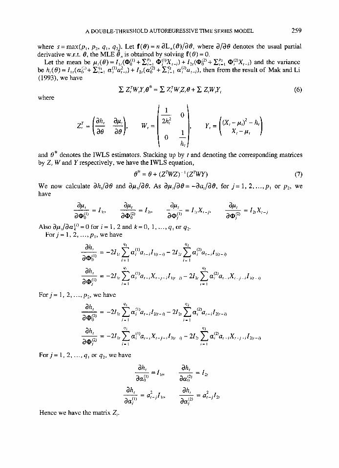
where s = max(p,, p2, q l , q2]. Let f(0) = n aL,,(e)/ae, where 8/86 denotes the usual partial derivative w.r.t. 8, the MLE 8, is obtained by solving f(0) = 0.
Let the mean be P I ( @ = Ilr(O#) + CpII Oj’)X,-;) + 12,(Oh2) + Zpzl Op12)X,-j) and the variance be h,(8) = I l r (a t )+ ZyLl a\”u~- i ) + 12,(ah2)+ C z I a$2)ur- i ) , then from the result of Mak and Li (1 993), we have
c z:w,r,e* = c z:w,z,e + C Z,W,Y, where
and 8” denotes the IWLS estimators. Stacking up by t and denoting the corresponding matrices by Z, Wand Y respectively, we have the IWLS equation,
(7)
We now calculate ah,/ae and ap,/ae. AS aPrlae= -au,/ae, for j = 1, 2, ..., p, or p 2 , we
ex = e + (z rwz) - I ( zTwr)
have
Also ap,/aap = o for i = 1, 2 and k = 0, 1, . . . , q1 or q2. For j = 1, 2, ..., p I , we have
For j = 1, 2, ..., p2, we have
For j = 1, 2, ..., q1 or q2, we have
Hence we have the matrix Z,.
260 C. \y. LI AND W. K. LI
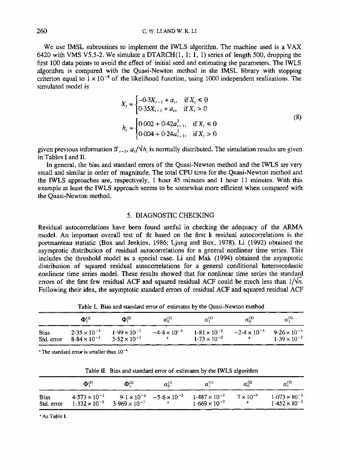
We use IMSL subroutines to implement the IWLS algorithm. The machine used is a VAX 6420 with VMS V5.5-2. We simulate a DTARCH(1, 1; 1, 1) series of length 500, dropping the first 100 data points to avoid the effect of initial seed and estimating the parameters. The IWLS algorithm is compared with the Quasi-Newton method in the IMSL library with stopping criterion equal to 1 x lo-' of the likelihood function, using 1000 independent realizations. The simulated model is
-0-3X,-, + (I,, if X , S 0 0.35X,-, + u,, if X , > 0
0.002 + 0.42~:- I , if X, s 0 h, = [ 0.004 + 0.24~:- if X , > 0
given previous information T,.-l, u,/dh, is normally distributed. The simulation results are given in Tables I and 11.
In general, the bias and standard errors of the Quasi-Newton method and the IWLS are very small and similar in order of magnitude. The total CPU time for the Quasi-Newton method and the IWLS approaches are, respectively, 1 hour 45 minutes and 1 hour 1 1 minutes. With this example at least the IWLS approach seems to be somewhat more efficient when compared with the Quasi-Newton method.
5 . DIAGNOSTIC CHECKING
Residual autocorrelations have been found useful in checking the adequacy of the ARMA model. An important overall test of fit based on the first k residual autocorrelations is the portmanteau statistic (Box and Jenkins, 1986; Ljung and Box, 1978). Li (1992) obtained the asymptotic distribution of residual autocorrelations for a general nonlinear time series. This includes the threshold model as a special case. Li and Mak (1994) obtained the asymptotic distribution of squared residual autocorrelations for a general conditional heteroscedastic nonlinear time series model. These results showed that for nonlinear time series the standard errors of the first few residual ACF and squared residual ACF could be much less than l/&. Following their idea, the asymptotic standard errors of residual ACF and squared residual ACF
Table I. Bias and standard error of estimates by the Quasi-Newton method
Bias 2.35 x 1.99 x lo-' -4.4 x 1-81 x -2.4 x lo-' 9.26 x lo-' Std. error 8.84 x lo-' 3.52 x 1.73 x 1.39 x lo-' d a
The standard error is smaller than
Table II. Bias and standard error of estimates by the IWLS algorithm
Bias 4.573 x lo-' 9.1 x -5.6 x 1.487 x lo-* 7 x 1.073 x Std. error 1.332 x 3.969 x lo-' d 1.669 x lo-* a 1.452 x
it As Table I.
A DOUBLE-THRESHOLD AUTOREGRESSIVE TIME SERIES MODEL 26 1
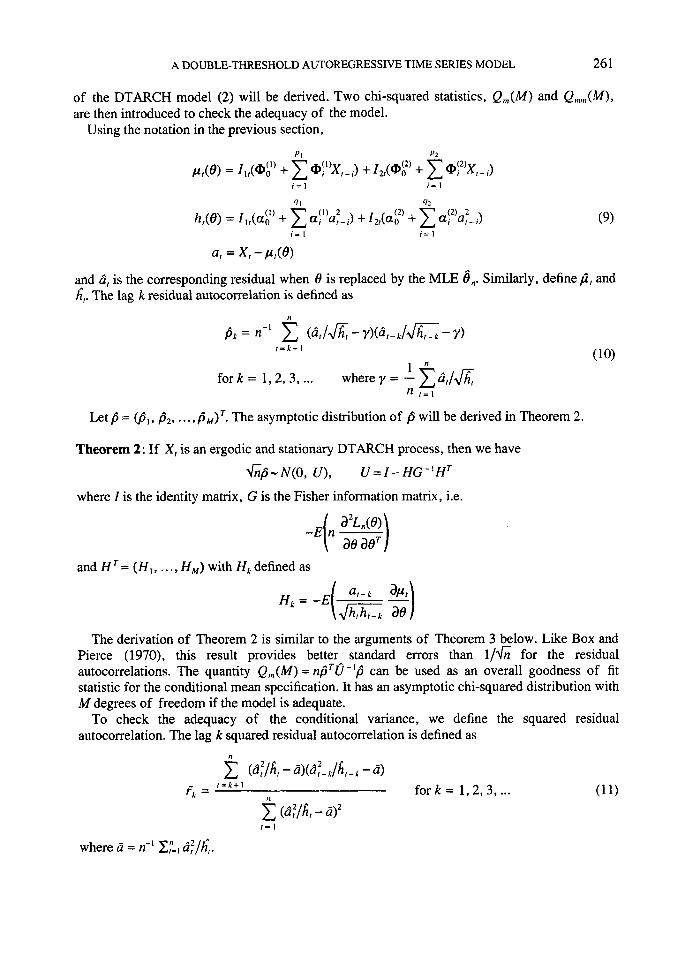
of the DTARCH model (2) will be derived. Two chi-squared statistics, Q,"(M) and Qnm(M), are then introduced to check the adequacy of the model.
Using the notation in the previous section,
1'1 YZ
i = 1 i = 1
'I I
i = 1 i = 1
at = Xr -
and d, is the corresponding residual when tl is replaced by the MLE 6,. Similarly, define k , and i,. The lag k residual autocorrelation is defined as
I = . k + l
1 "
n , = I
fork = 1,2,3, ... where y = - c &,/A
Let p = u 1 , pz, . . . , pM)'. The asymptotic distribution of p will be derived in Theorem 2.
Theorem 2: If X , is an ergodic and stationary DTARCH process, then we have
Gp- N ( 0 , U ) , U = I - HG-'HT
where Z is the identity matrix, G is the Fisher information matrix, i.e.
and H T = (HI, ..., H,,,) with H,defined as
The derivation of Theorem 2 is similar to the arguments of Theorem 3 below. Like Box and Pierce (1970), this result provides better standard errors than l / f i for the residual autocorrelations. The quantity Q,(M) = npT0-'@ can be used as an overall goodness of fit statistic for the conditional mean specification. It has an asymptotic chi-squared distribution with M degrees of freedom if the model is adequate.
To check the adequacy of the conditional variance, we define the squared residual autocorrelation. The lag k squared residual autocorrelation is defined as
262 C . W. LI AND W. K. LI
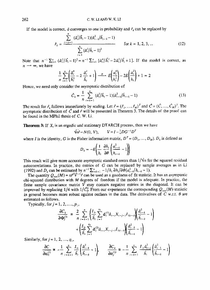
If the model is correct, c i converges to one in probability and f k can be replaced by n 1 (d;/hr- l)(d;-,/hr-L- 1)
c (d:/hr - 1)' I!
fork = 1,2, 3, ... (12) A r = t + l rL =
r = 1
Note that n-' x:=, (d,?/Gr - 1)*= n-' Z:=, [d : /@ - 2d:/h", + 11. If the model is correct, as n - 00, we have
Hence, we need only consider the asymptotic distribution of
The result for tk follows immediately by scaling. Let i = (i,, . . . , iM) and c = (c, . . . , c,,,) '. The asymptotic distribution of c and t will be presented in Theorem 3. The details of the proof can be found in the MPhil thesis of C. W. Li.
Theorem 3: If X, is an ergodic and stationary DTARCH process, then we have
where I is the identity, G is the Fisher information matrix, D T = ( D l , . . . , D,,,). D, is defined as G~-N(o , v), V = I - : D G - ' D ~
This result will give more accurate asymptotic standard errors than 1/dn for the squared residual autocorrelations. In practice, the entries of G can be replaced by sample averages as in Li (1992) and D,can beestimated by n-'C:=,+, - l / h r ahr/aB(a:-k/h,-L- 1).
The quantity Q m ( M ) = n F T v - ' t can be used as a goodness of fit statistic. It has an asymptotic chi-squared distribution with M degrees of freedom if the model is adequate. In practice, the finite sample covariance matrix v may contain negative entries in the diagonal. It can be improved by replacing 1/4 with l / e i . From our experience the corresponding Q,,,,(M) statistic in general becomes more robust against outliers in the data. The derivatives of C w.r.t. 8 are estimated as follows.
Typically, for j = 1 , 2, . . .., p , ,
Similarly, f o r j = 1, 2, ..., q , ,
A DOUBLE-THRESHOLD AUTOREGRESSIVE TIME SERIES MODEL 263
The vector D, is then estimated by stacking together ae,/d@t), JeL/&D{’), . . ., de,/a@1,22! a(?,/ sat), ae,/&$), . . . , aC,/aa$
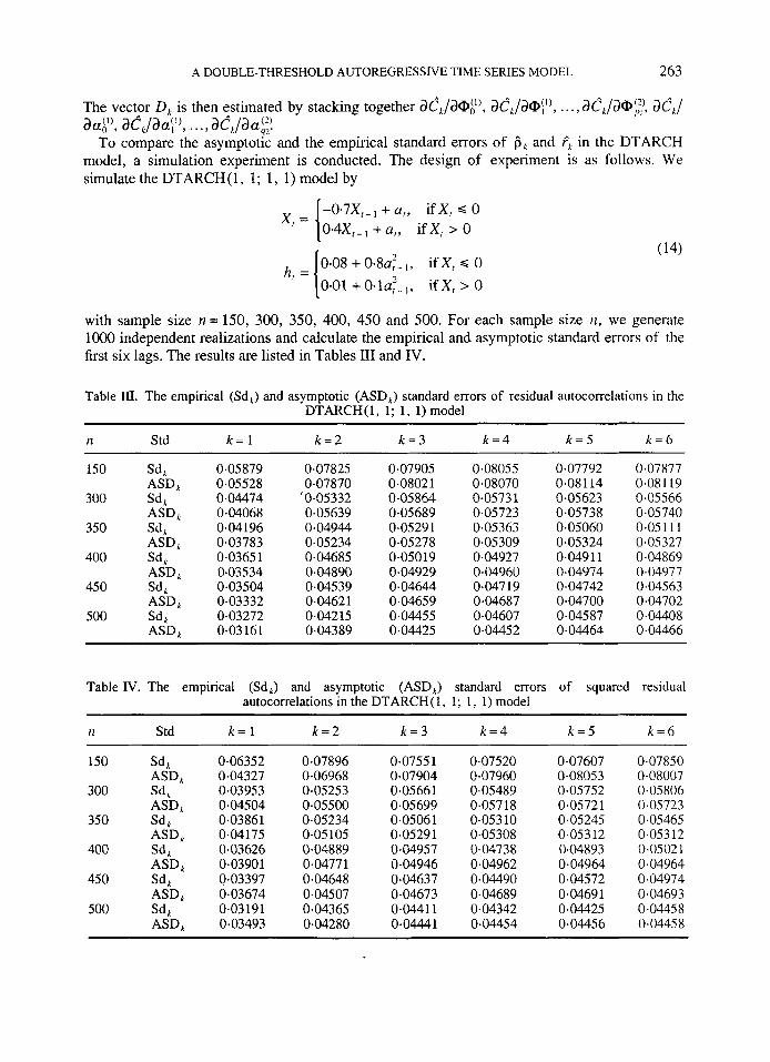
To compare the asymptotic and the empirical standard errors of 6, and t, in the DTARCH model, a simulation experiment is conducted. The design of experiment is as follows. We simulate the DTARCH (1, 1 ; 1, 1) model by
-o.~X,-, + a,, ifX, s 0 0.4X,-, +a,, ifX, > 0
with sample size n = 150, 300, 350, 400, 450 and 500. For each sample size n , we generate lo00 independent realizations and calculate the empirical and asymptotic standard errors of the first six lags. The results are listed in Tables 111 and IV.
Table III. The empirical (Sd,) and asymptotic (ASD,) standard errors of residual autocorrelations in the DTARCH(1, 1; 1, 1) model
I 2 Std k = 1 k = 2 k = 3 k = 4 k = 5 k = 6
150 Sd,
300 Sd,
350 Sd,
400 Sd,
450 Sd,
ASD,
ASD , ASD,
ASD , ASD,
ASD , 500 Sd I
0.05879 0.05528 0.04474 0.04068 0.04196 0.03783 0.0365 1 0.03534 0.03504 0.03332 0.03272 0.03161
0.07825 0.07870
‘0.05332 0.05639 0.04944 0.05234 0.04685 0.04890 0.04539 0.0462 1 0.04215 0.04389
0.07905 0.08021 0.05864 0.05689 0.05291 0.05278 0.05019 0-04929 0.04644 0.04659 0.04455 0.04425
0.08055 0.08070 0.0573 1 0.05723 0.05363 0.05309 0.04927 0.04960 0.047 19 0.04687 0.04607 0.0445 2
0.07792 0.081 14 0.05623 0.05738 0.05060 0.05 3 24 0.049 1 1 0.04974 0.04742 0.04700 0.04587 0.04464
0.07877 0.08119 0-05566 0.05740 0.05111 0.05327 0.04869 0.04977 0.04563 0.04702 0.04408 0.04466
Table IV. The empirical (Sd,) and asymptotic (ASD,) standard errors of squared residual autocorrelations in the DTARCH(1, 1; 1, 1) model
~ ~~~ ~ ~~
I 2 Std k = l k = 2 k = 3 k = 4 k = 5 X=6
150 Sd A
300 Sd A
350 Sd,
400 Sd,
450 Sd,
ASD,
ASD,
ASD,
ASD,
ASD,
ASD, 500 Sd I
0.06352 0.04327 0.03953 0.04504 0.03861 0.04175 0.03626 0.03901 0.03397 0.03674 0.03 191 0.03493
0.07896 0.06968 0.05253 0.05500 0.05234 0.05 105 0.04889 0.04771 0.04648 0.04507 0.04365 0.04280
0.0755 1 0-07904 0.05661 0.05699 0.05061 0.05291 0.04957 0.04946 0.04637 0,04673 0.0441 1 0.04441
0.07520 0.07960 0-05489 0.05718 0.05310 0.05308 0-04738 0.04962 0.04490 0.04689 0.04342 0.04454
0.07607 0-08053 0.05752 0.05721 0.05245 0.05312 0.04893 0.04964 0.04572 0.04691 0.04425 0.04456
0.07850 0.08007 0.05806 0.05723 0.05465 0.05312 0.0502 f 0.04964 0.04974 0.04693 0.04458 0.04458
264 C. W. LI AND W. K. LI
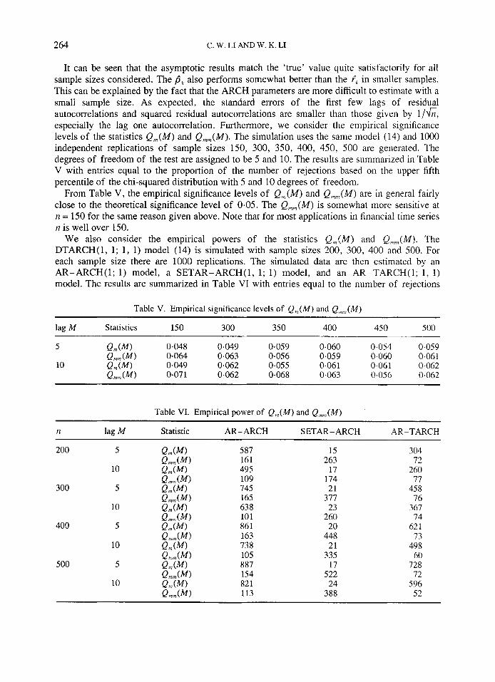
It can be seen that the asymptotic results match the 'true' value quite satisfactorily for all sample sizes considered. The pk also performs somewhat better than the tk in smaller samples. This can be explained by the fact that the ARCH parameters are more difficult to estimate with a small sample size. As expected, the standard errors of the first few lags of residual autocorrelations and squared residual autocorrelations are smaller than those given by 1 /fi, especially the lag one autocorrelation. Furthermore, we consider the empirical significance levels of the statistics Q,n(M) and Q,n,n(M). The simulation uses the same model (14) and 1000 independent replications of sample sizes 150, 300, 350, 400, 450, 500 are generated. The degrees of freedom of the test are assigned to be 5 and 10. The results are summarized in Table V with entries equal to the proportion of the number of rejections based on the upper fifth percentile of the chi-squared distribution with 5 and 10 degrees of freedom.
From Table V, the empirical significance levels of Q,,(M) and Q,n,,,(M) are in general fairly close to the theoretical significance level of 0.05. The Q,,n(M) is somewhat more sensitive at n = 150 for the same reason given above. Note that for most applications in financial time series n is well over 150.
We also consider the empirical powers of the statistics Q,n(M) and Q,,,,,,(M). The DTARCH(1, 1; 1, 1) model (14) is simulated with sample sizes 200, 300, 400 and 500. For each sample size there are 1000 replications. The simulated data are then estimated by an AR-ARCH(1; 1) model, a SETAR-ARCH(1, 1; I ) model, and an AR-TARCH(1; 1, 1) model. The results are summarized in Table VI with entries equal to the number of rejections
Table V. Empirical significance levels of Q,,(M) and Q,","(M)
lag M Statistics 150 300 350 400 450 500
5 Q,,(MI 0.048 0.049 0.059 0.060 0.054 0.059 Q,,,, (MI 0.064 0.063 0.056 0.059 0.060 0.061
10 Q,,(W 0.049 0,062 0.055 0.06 1 0.06 1 0.062 Q,,,, (MI 0.07 1 0.062 0.068 0.063 0.056 0.062
~~~
Table VI. Empirical power of Q,,(M) and Q,,,,(M)
I1 lag M Statistic AR-ARCH SETAR-ARCH AR-TARCH
200 5
10
300 5
10
400 5
10
500 5
10
587 161 495 109 745 165 638 10 1 861 163 738 105 887 154 82 1 113
15 263
17 174 21
377 23
260 20
448 21
335 17
522 24
388
304 72
260 77
45 8 76
367 74
62 1 73
498 60
728 72
596 52
A DOUBLE-THRESHOLD AUTOREGRESSIVE TIME SERIES MODEL 265
based on the upper fifth percentiles of the chi-squared distributions with 5 and 10 degrees of freedom.
It can be seen that except for situations explained below, in general the empirical powers are not large when n = 200, but they improve if the sample size grows to 400 or 500. The empirical powers when M = 5 is larger than those when M = 10. This is not surprising, as the first few autocorrelations are usually more informative (Ansley and Newbold, 1979) than the others. For the SETAR-ARCH model, model misspecification occurred in the conditional variance; and for the AR-TARCH model, model misspecification occurred in the conditional mean. These explain why the empirical powers of Q,n(M) for the SETAR-ARCH model and Q,,,,,(M) for the AR-TARCH model are small, since part of the behavior of the DTARCH model have been taken into consideration. For the AR-ARCH model, model misspecifications are in both the conditional mean and the conditional variance. The empirical powers of Q,,,(M) are quite high for all cases, but the empirical powers of Q,,,,(M) are small even when n = 500. These suggest that if both conditional mean and conditional variance are misspecified, the misspecification of the conditional mean may spoil the power of Q,,(M). This in fact provides a justification for the modelling procedure proposed in Section 3. When fitting the DTARCH model, the conditional mean specification should be checked first. After the conditional mean is correctly specified, there are fewer problems with the power of Q,,,,(M) and the correct identification of the conditional variance structure. Note that given a correct conditional mean specification, estimates for @,(j) will still be consistent although inefficient.
6. EMPIRICAL RESULTS
It is a market belief that stock prices in a bull market behaves differently from that in a bear market. See Karpoff (1987) for a comprehensive review. This kind of distributional differences between bull and bear market could be described by nonlinearity in both the conditional mean and the conditional variance. This phenomenon can be modelled easily by the DTARCH model.
As an illustration, the DTARCH(y,, p2; q , , q2) model will be applied to the daily Hong Kong Hang Seng Index (HSI) from 1982 to 1991. The return series is defined as the log difference of the index. As the situation in Hong Kong has undergone a dramatic change within the ten years it is reasonable to believe that the structure of the market evolves over time. Therefore it may be reasonable to divide the data into ten non-overlapping time periods. We used one year as a period and in each period there are about 245 observations. Using the identification scheme in Section 3, we found that it is adequate to assume that r = 0 and d = 1. This choice of the threshold and delay parameters is consistent with observations on the stock market.
Refinement of AR orders and ARCH orders are achieved using AIC and the portmanteau statistics. All the models are estimated by the IWLS procedure of Section 4. To reduce the number of possible models, it is assumed that y , = p 2 = p and q , = q2 = q. Table VII presents the final fitted orders of the DTARCH model. The corresponding estimates (with @:) and restricted to zero) can be found in the Appendix. As a further check on the final DTARCH model likelihood ratio statistics can be computed for restrictions on igcJ) and a(’). However, in order to have a valid chi-squared test it is necessary to assume known threshold and delay parameters. It is, in principle, possible to develop tests without assuming known threshold and delay parameters along the lines of Chan and Tong (1990) and Chan (1990). Nevertheless, this seems to be beyond the scope of the present paper. As in the SETAR case (Chan and Tong, 1990), the likelihood ratio tests considered here may have a much larger significance level when compared with more general tests not assuming known threshold structure.
One interesting rival to the full DTARCH model is the original SETAR model of Tong and Lim
266 C. W. LI AND W. K. LI
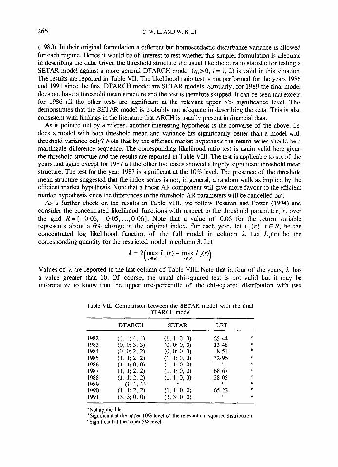
(1980). In their original formulation a different but homoscedastic disturbance variance is allowed for each regime. Hence it would be of interest to test whether this simpler formulation is adequate in describing the data. Given the threshold structure the usual llkelihood ratio statistic for testing a SETAR model against a more general DTARCH model ( q i > O , i = 1, 2) is valid in this situation. The results are reported in Table VII. The likelihood ratio test is not performed for the years 1986 and 1991 since the final DTARCH model are SETAR models. Similarly, for 1989 the final model does not have a threshold mean structure and the test is therefore skipped. It can be seen that except for 1986 all the other tests are significant at the relevant upper 5% significance level. This demonstrates that the SETAR model is probably not adequate in describing the data. This is also consistent with findings in the literature that ARCH is usually present in financial data.
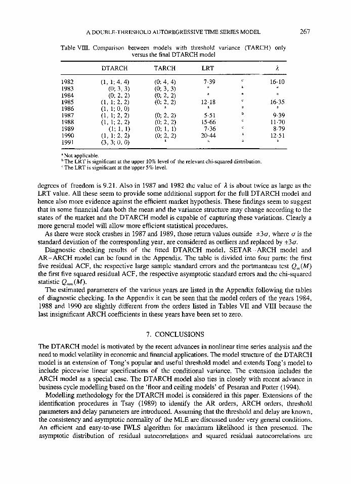
As is pointed out by a referee, another interesting hypothesis is the converse of the above: i.e. does a model with both threshold mean and variance fits significantly better than a model with threshold variance only? Note that by the efficient market hypothesis the return series should be a martingale difference sequence. The corresponding likelihood ratio test is again valid here given the threshold structure and the results are reported in Table VIII. The test is applicable to six of the years and again except for 1987 all the other five cases showed a highly significant threshold mean structure. The test for the year 1987 is significant at the 10% level. The presence of the threshold mean structure suggested that the index series is not, in general, a random walk as implied by the efficient market hypothesis. Note that a linear AR component will give more favour to the efficient market hypothesis since the differences in the threshold AR parameters will be cancelled out.
As a further check on the results in Table VIII, we follow Pesaran and Potter (1994) and consider the concentrated likelihood functions with respect to the threshold parameter, r , over the grid R = [-0.06, -0.05, ..., 0.061. Note that a value of 0.06 for the return variable represents about a 6% change in the original index. For each year, let f , , ( r ) , r E R , be the concentrated log likelihood function of the full model in column 2. Let L 2 ( r ) be the corresponding quantity for the restricted model in column 3. Let
1 = 2 max L,(r ) - max L2(r) ( r E R r E R
Values of 1 are reported in the last column of Table VIII. Note that in four of the years, 1 has a value greater than 10. Of course, the usual chi-squared test is not valid but it may be informative to know that the upper one-percentile of the chi-squared distribution with two
Table VII. Comparison between the SETAR model with the final DTARCH model
DTARCH
1982 1983 1984 1985 1986 1987 1988 1989 1990 1991
LRT
65-44 13.48 8.51
32.96
68.67 28.05
65.23
c
b
C
a d
‘ c
‘I d
c
a a
-
Not applicable. hSignificant at the upper 10% level of the relevant chi-squared distribution. “Significant at the upper 5% level.
A DOUBLE-THRESHOLD AUTOREGRESSIVE TIME SERIES MODEL 267
Table VIII. Comparison between models with threshold variance (TARCH) only versus the final DTARCH model
DTARCH TARCH LRT A c
d a d 1982 (1, 1; 4,4) (0; 4, 4) 7.39 16.10 1983 (0; 3, 3) (0; 3, 3) 1984 (0; 2, 2) (0; 2, 2)
1986 (1, 1; 0,O)
a a a
c 16.35
9.39 11.70 8.79
12.5 1
1985 (1, 1; 2, 2) (0; 2, 2) 12.18
1987 (1, 1; 2 ,2 ) (0; 2, 2) 5.51 1988 (1, 1; 2 ,2) (0; 2, 2) 15.66 1989 (1; 1, 1) (0; 1, 1) 7.36
a h a d
b
c
c
d 1990 (1, 1; 2 ,2 ) (0; 2, 2) 20.44 1991 (3, 3; 0, 0 ) a a il a
a Not applicable. hThe LRT is significant at the upper 10% level of the relevant chi-squared distribution. ‘The LRT is significant at the upper 5% level.
degrees of freedom is 9.21. Also in 1987 and 1982 the value of A is about twice as large as the LRT value. All these seem to provide some additional support for the full DTARCH model and hence also more evidence against the efficient market hypothesis. These findings seem to suggest that in some financial data both the mean and the variance structure may change according to the states of the market and the DTARCH model is capable of capturing these variations. Clearly a more general model will allow more efficient statistical procedures.
As there were stock crashes in 1987 and 1989, those return values outside k30, where cr is the standard deviation of the corresponding year, are considered as outliers and replaced by k30.
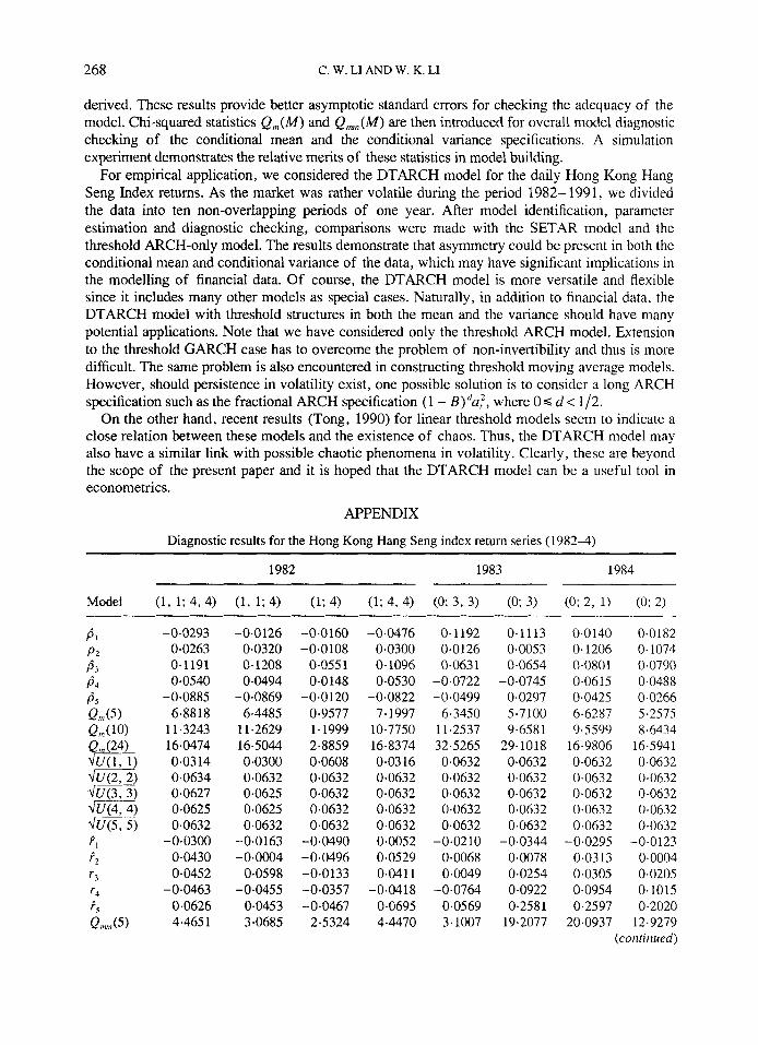
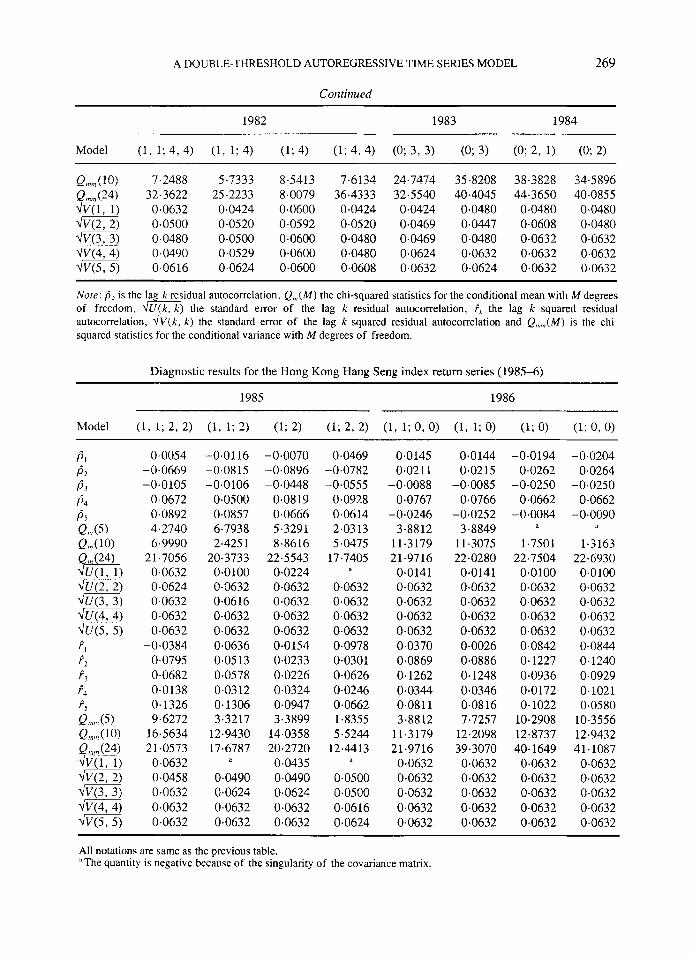
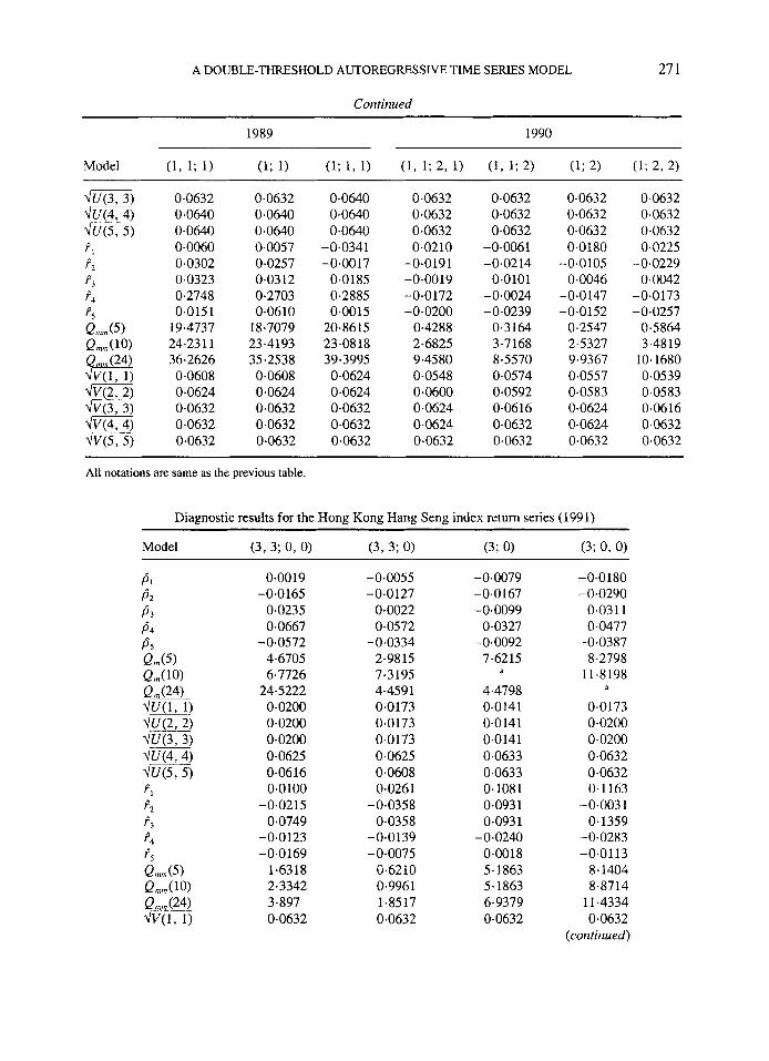
Diagnostic checking results of the fitted DTARCH model, SETAR-ARCH model and AR-ARCH model can be found in the Appendix. The table is divided into four parts: the first five residual ACF, the respective large sample standard errors and the portmanteau test Q,n(M) the first five squared residual ACF, the respective asymptotic standard errors and the chi-squared statistic Qmm(M).
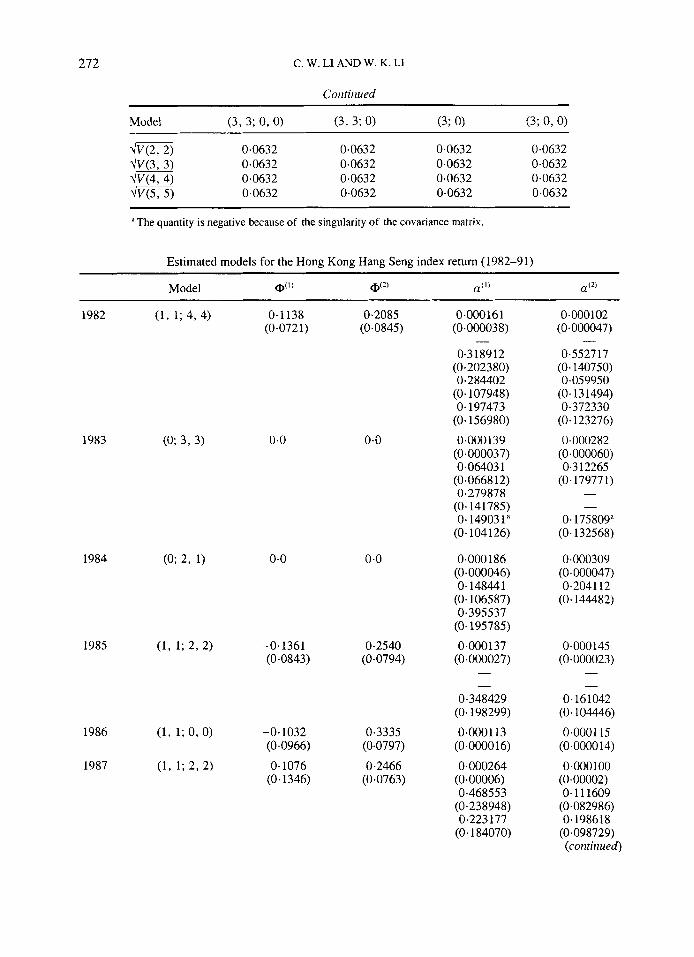
The estimated parameters of the various years are listed in the Appendix following the tables of diagnostic checking. In the Appendix it can be seen that the model orders of the years 1984, 1988 and 1990 are slightly different from the orders listed in Tables VII and VIII because the last insignificant ARCH coefficients in these years have been set to zero.
7. CONCLUSIONS
The DTARCH model is motivated by the recent advances in nonlinear time series analysis and the need to model volatility in economic and financial applications. The model structure of the DTARCH model is an extension of Tong’s popular and useful threshold model and extends Tong’s model to include piecewise linear specifications of the conditional variance. The extension includes the ARCH model as a special case. The DTARCH model also ties in closely with recent advance in business cycle modelling based on the ‘floor and ceiling models’ of Pesaran and Potter (1994).
Modelling methodology for the DTARCH model is considered in this paper. Extensions of the identification procedures in Tsay (1989) to identify the AR orders, ARCH orders, threshold parameters and delay parameters are introduced. Assuming that the threshold and delay are known, the consistency and asymptotic normality of the MLE are discussed under very general conditions. An efficient and easy-to-use IWLS algorithm for maximum likelihood is then presented. The asymptotic distribution of residual autocorrelations and squared residual autocorrelations are
268 C. W. LI AND W. K. LI
derived. These results provide better asymptotic standard errors for checking the adequacy of the model. Chi-squared statistics Q,,(M) and Q,,,,,(M) are then introduced for overall model diagnostic checking of the conditional mean and the conditional variance specifications. A simulation experiment demonstrates the relative merits of these statistics in model building.
For empirical application, we Considered the DTARCH model for the daily Hong Kong Hang Seng Index returns. As the market was rather volatile during the period 1982- 1991, we divided the data into ten non-overlapping periods of one year. After model identification, parameter estimation and diagnostic checking, comparisons were made with the SETAR model and the threshold ARCH-only model. The results demonstrate that asymmetry could be present in both the conditional mean and conditional variance of the data, which may have significant implications in the modelling of financial data. Of course, the DTARCH model is more versatile and flexible since it includes many other models as special cases. Naturally, in addition to financial data, the DTARCH model with threshold structures in both the mean and the variance should have many potential applications. Note that we have considered only the threshold ARCH model. Extension to the threshold GARCH case has to overcome the problem of non-invertibility and thus is more difficult. The same problem is also encountered in constructing threshold moving average models. However, should persistence in volatility exist, one possible solution is to consider a long ARCH specification such as the fractional ARCH specification (1 - B)"u;, where 0 G d < 1/2.
On the other hand, recent results (Tong, 1990) for linear threshold models seem to indicate a close relation between these models and the existence of chaos. Thus, the DTARCH model may also have a similar link with possible chaotic phenomena in volatility. Clearly, these are beyond the scope of the present paper and it is hoped that the DTARCH model can be a useful tool in econometrics.
APPENDIX
Diagnostic results for the Hong Kong Hang Seng index return series (19824)
1982 1983 1984
Model (1, 1; 4, 4) (1, 1; 4) (I; 4) (1; 4, 4) (0; 3, 3) (0; 3) (0; 2, 1) (0; 2)
-0.0293 0.0263 0.1191 0.0540
-0.0885 6.8818
11.3243 160374 0,0314 0.0634 0.0627 0.0625 0.0632
-0.0300 0.0430 0.0452
-0.0463 0.0626 4.465 1
-0.0126 0.0320 0- 1208 0.0494
-0.0869 6.4485
11.2629 16.5044 0.0300 0.0632 0.0625 0.0625 0.0632
-0.0163 -0.0004
0.0598 -0.0455
0.0453 3.0685
-0.0160 -0.0108
0-055 1 0.0148
-0.0120 0.9577 1.1999 2.8859 0.0608 0.0632 0.0632 0.0632 0.0632
-0.0490 -0.0496 -0.0133 -0.0357 -0.0467
2.5324
-0.0476 0.0300 0-1096 0.0530
-0.0822 7.1997
10.7750 16.83 74 0.0316 0.0632 0.0632 0,0632 0,0632 0.0052 0.0529 0.041 1
- 0.04 1 8 0.0695 4.4470
0.1 192 0.0126 0.063 1
-0.0722 -0.0499
6.3450 11.2537 32.5265 0.0632 0.0632 0.0632 0.0632 0.0632
-0.0210 0.0068 0.0049
-0.0764 0.0569 3.1007
0.1113 0.0053 0.0654
-0.0745 -0.0297
5.7100 9.6581
29.1018 0.0632 0.0632 0.0632 0.0632 0.0632
-0.0344 0.0078 0.0254 0.0922 0.2581
19.2077
0.0140 0.0182 0.1206 0.1074 0.0801 0.0790 0.0615 0.0488
-0.0425 -0.0266 6.6287 5.2575 9.5599 8.6434
16.9806 165941 0.0632 0.0632 0.0632 0.0632 0.0632 0.0632 0.0632 0.0632 0.0632 0.0632
-0.0295 -0.0123 0.03 13 0.0004 0.0305 0.0205 0.0954 0.1015 0.2597 0.2020
20.0937 12.9279 (confirmed)
A DOUBLE-THRESHOLD AUTOREGRESSIVE TIME SERIES MODEL 269
Coiitiriued
1982 1983 1984
Model (1, 1; 4, 4) (1, 1; 4) (1; 4) (1; 4 ,4 ) (0; 3, 3) (0; 3) (0; 2, 1) (0; 2)
Q,,(lO) 7.2488 5.7333 8.5413 7.6134 24.7474 35.8208 38.3828 34.5896 Q (24) 32.3622 25.2233 8.0079 36.4333 32.5540 40.4045 44.3650 40.0855
m) 0.0500 0.0520 0.0592 0.0520 0.0469 0.0447 0.0608 0.0480 7Jv(3,3) 0.0480 0.0500 0.0600 0.0480 0.0469 0.0480 0.0632 0.0632 mq 0.0490 0.0529 0.0600 0.0480 0.0624 0.0632 0.0632 0.0632 m) 0.0616 0.0624 0.0600 0.0608 0.0632 0.0624 0.0632 0.0632
a) 0.0632 0.0424 0.0600 0.0424 0.0424 0.0480 0.0480 0.0480
Nore: b, is the la k residual autocorrelation, Q,,,(M) the chi-squared statistics for the conditional mean with M degrees
autocorrelation, .Iv(x-,) the standard error of the lag k squared residual autocorrelation and Q,,,,,,(M) is the chi- squared statistics for the conditional variance with M degrees of freedom.
of freedom, + U ( k , k ) the standard error of the lag k residual autocorrelation, F, the lag k squared residual
Diagnostic results for the Hong Kong Hang Seng index return series (1985-6)
1985 1986
Model (1, 1; 2, 2) (1, 1; 2) (1; 2) (1; 2, 2) (1, 1; 0, 0) (1, 1; 0) (1; 0) (1; 0, 0)
0.0054 - 0-0669 -0.0105
0.0672 0.0892 4.2740 6.9990
21.7056 0-0632 0.0624 0.0632 0.0632 0-0632
-0.0384 0.0795 0.0682 0.0138 0.1326 9.6272
16.5634 21-0573 0.0632 0.0458 0.0632 0.0632 0.0632
-0.0116 -0.0815 -0.0106
0.0500 0.0857 6.7938 2.425 1
20.3733 0~0100 0.0632 0.0616 0.0632 0.0632 0.0636 0.05 13 0.0578 0.0312 0.1306 3.3217
12.9430 17.6787
d
0.0490 0.0624 0.0632 0.0632
-0.0070 -0.0896 -0.0448
0.0819 0.0666 5.3291 8.8616
22.5 543 0.0224 0.0632 0.0632 0.0632 0.0632 0.0154 0.0233 0.0226 0.0324 0.0947 3.3899
14.0358 20.2720 0.0435 0.0490 0.0624 0.0632 0.0632
0.0469 -0.0782 -0.0555
0.0928 0.0614 2.0313 5.0475
17.7405
0.0632 0.0632 0.0632 0.0632 0.0978 0.0301 0.0626 0.0246 0.0662 1.8355 5.5244
12.4413
0.0500 0.0500 0.0616 0.0624
P
0.0145 0.021 1
-0.0088 0.0767
-0.0246 3.8812
11.3179 21.9716 0.0141 0.0632 0.0632 0-0632 0.0632 0.0370 0.0869 0.1262 0.0344 0.08 1 1 3.8812
11.3179 2 1.97 16 0,0632 0.0632 0.0632 0.0632 0.0632
0-0144 0.0215
-0.0085 0.0766
-0.0252 3.8849
11.3075 22.0280 0.0141 0.0632 0.0632 0.0632 0.0632 0.0026 0.0886 0.1248 0.0346 0.0816 7.7257
12.2098 39.3070 0.0632 0.0632 0,0632 0.0632 0.0632
-0.0194 0.0262
-0.0250 0.0662
- 0.0084 'I
1.7501 22.7504
0~0100 0-0632 0.0632 0.0632 0.0632 0.0842 0.1227 0.0936 0.0172 0.1022
10.2908 12.8737 40.1649
0.0632 0.0632 0.0632 0.0632 0.0632
-0.0204 0.0264
-0.0250 0.0662
-0.0090 il
1.3163 22.6930 0~0100 0-0632 0.0632 0.0632 0.0632 0.0844 0.1240 0.0929 0.1021 0.0580
10.3556 12.9432 41.1087
0.0632 0-0632 0-0632 0.0632 0.0632
All notations are same as the previous table. "The quantity is negative because of the singularity of the covariance matrix.
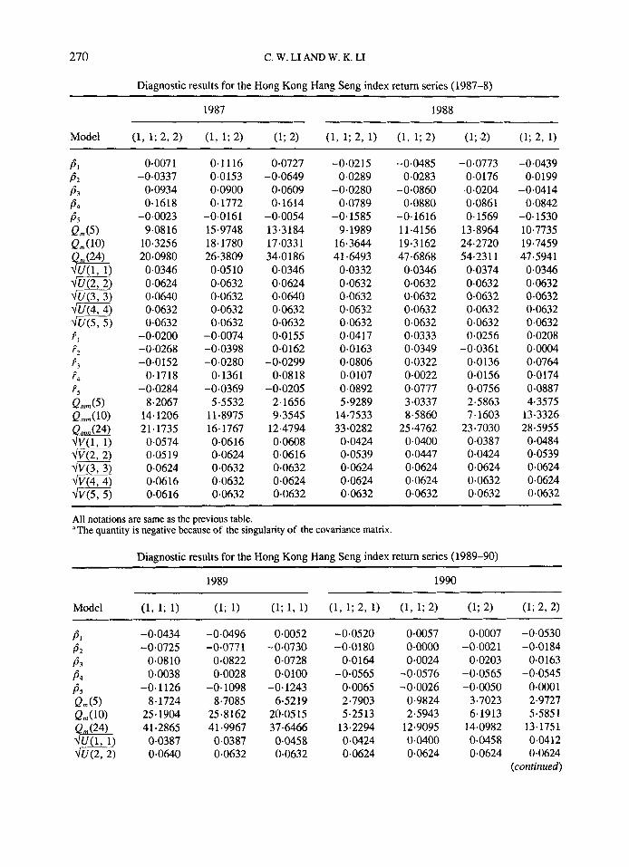
270 C. W. LI AND W. K. LI
Diagnostic results for the Hong Kong Hang Seng index return series (1987-8)
1987 1988
Model (1, 1; 2, 2) (1, 1; 2) (1; 2) (1, 1; 2, 1) (1, 1; 2) (1 ;a (1; 2, 1)
0.007 1 -0.0337
0.0934 0.1618
-0.0023 9.0816
10.3256 20.0980 0.0346 0.0624 0.0640 0.0632 0-0632
-0.0200 -0.0268 -0.0152
0.1718 -0.0284
8.2067 14.1206 21.1735 0.0574 0.0519 0.0624 0.0616 0.0616
0.1116 0.0153 0.0900 0.1772
-0.0161 15.9748 18.1780 26.3809 0.0510 0.0632 0.0632 0.0632 0.0632
-0.0074 -0.0398 -0.0280
0.1361 -0.0369
5.5532 11.8975 16.1767 0.0616 0.0624 0.0632 0.0632 0.0632
0.0727 -0.0649
0.0609 0.1614
- 0.0054 13.3184 17.0331 34.0 186 0.0346 0.0624 0.0640 0.0632 0.0632 0.0155 0.0162
-0.0299 0.08 18
-0.0205 2.1656 9.3545
12.4794 0.0608 0.0616 0.0632 0.0624 0.0632
-0.0215 0.0289
-0.0280 0.0789
-0.1585 9.1989
16.3644 41.6493 0.0332 0.0632 0.0632 0.0632 0.0632 0.0417 0.0163 0.0806 0.0107 0.0892 5.9289
14-7533 33.0282 0.0424 0.0539 0-0624 0.0624 0.0632
-0.0485 0.0283
-0.0860 0.0880
-0.1616 11.4156 19.3162 47.6868 0.0346 0.0632 0.0632 0.0632 0.0632 0.0333 0.0349 0.0322 0.0022 0.0777 3.0337 8.5860
25 *4762 0.0400 0.0447 0.0624 0.0624 0.0632
-0.0773 0-0176
-0.0204 0.0861 0.1569
13.8964 24.2720 54.23 1 1 0.0374 0.0632 0.0632 0.0632 0.0632 0.0256
-0.0361 0.0136 0.0156 0.0756 2.5863 7.1603
23.7030 0.0387 0.0424 0.0624 0.0632 0.0632
-0.0439 0.0199
-0.0414 0.0842
-0.1530 10.7735 19.7459 47.5941 0.0346 0.0632 0.0632 0.0632 0.0632 0.0208 0.0004 0.0764 0.0174 0.0887 4.3575
13.3326 28.5955 0.0484 0.0539 0.0624 0.0624 0.0632
All notations are same as the previous table. 'The quantity is negative because of the singularity of the covariance matrix.
Diagnostic results for the Hong Kong Hang Seng index return series (1989-90)
PI -0.0434 P 2 -0.0725
P 4 0.0038 P5 -0.1126 Qm(5) 8.1724 Q,n (1 0) 25.1904
41.2865
P 3 0.0810
e) 0.0387 4m-T) 0.0640
-0.0496 -0.077 1
0.0822 0.0028
-0.1098 8.7085
25 -8 162 41.9967 0.0387 0.0632
0.0052 - 0.07 30
0-0728 0*0100
-0.1243 6.5219
20.05 15 37.6466 0.0458 0.0632
-0.0520 -0.0180
0.0164 -0.0565
0.0065 2.7903 5.2513
13.2294 0-0424 0.0624
0.0057 0~0000 0.0024
-0.0576 -0.0026
0.9824 2.5943
12.9095 0.0400 0.0624
0.0007 -0,0021
0.0203 - 0.05 65 -0.0050
3.7023 6.1913
14.0982 0.0458 0.0624
-0.0530 -0.0184
0.0163 -0.0545
0~000 1 2.9727 5.585 1
13.1751 0,0412 0.0624
(continued)
A DOUBLE-THRESHOLD AUTOREGRESSIVE TIME SERIES MODEL 27 1
0.0632 0.0640 0.0640 0.0060 0.0302 0.0323 0.2748 0.0151
19.4737 24.23 1 1 36.2626 0.0608 0.0624 0.0632 0.0632 0.0632
0.0632 0.0640 0.0640 0.0057 0.0257 0.0312 0.2703 0.0610
18.7079 23.4193 35.2538 0.0608 0.0624 0.0632 0.0632 0.0632
0.0640 0.0640 0,0640
-0.0341 -0.0017
0.0185 0.2885 0.0015
20.86 15 23.0818 39.3995 0.0624 0.0624 0.0632 0.0632 0.0632
0.0632 0.0632 0.0632 0.0210
-0.0191 -0.0019 -0.0172 -0-0200
0-4288 2-6825 9.4580 0.0548 0.0600 0.0624 0-0624 0.0632
0.0632 0.0632 0.0632
-0-0061 -0.0214
0.0101 -0.0024 -0.0239
0.3164 3.7168 8.5570 0.0574 0.0592 0.06 16 0-0632 0.0632
0.0632 0.0632 0.0632 0.0180
-0.0105 0.0046
-0.0147 -0.0152
0.2547 2.5327 9.9367 0.0557 0.0583 0.0624 0.0624 0.0632
0.0632 0.0632 0.0632 0.0225
-0.0229 0.0042
-0.0173 -0.0257
0.5864 3.4819
10.1680 0.0539 0.0583 0.0616 0.0632 0.0632
All notations are same as the previous table.
Diagnostic results for the Hong Kong Hang Seng index return series (1991)
P I
d2
P 3
P 4
ds Q,,(5>
0.0019 -0.0165
0.0235 0-0667
-0.0572 4.6705 6.7726
24.5222 0.0200 0.0200 0.0200 0.0625 0.0616 0~0100
-0.0215 0.0749
-0.0123 -0.0169
1.6318 2.3342 3.897 0.0632
-0.0055 - 0.0 127
0.0022 0.0572
-0.0334 2.9815 7.3195 4.459 1 0.0173 0.0173 0.0173 0.0625 0,0608 0.0261
-0,0358 0.0358
-0.0139 -0.0075
0.62 10 0.9961 1.8517 0,0632
-0.0079 -0.0167 -0.0099
0.0327 -0.0092
7.6215 a
4.4798 0.0141 0.0141 0.0141 0.0633 0.0633 0.108 1 0.093 1 0.093 1
-0.0240 0.0018 5-1863 5.1863 6.9379 0.0632
-0.0180 -0.0290
0.031 1 0.0477
-0.0387 8.2798
11.8198 a
0.0173 0~0200 0.0200 0.0632 0.0632 0.1163
-0.003 1 0.1359
-0.0283 -0.0113
8.1404 8.8714
11.4334 0.0632
(coiztirzued)
272 C. W. LI AND W. K. LI
Coritiriued
llvo 0.0632 0.0632 0.0632 0.0632 q 3 7 ) 0.0632 0.0632 0.0632 0.0632 -1 0.0632 0.0632 0.0632 0.0632 -1 0.0632 0.0632 0.0632 0.0632
The quantity is negative because of the singularity of the covariance matrix.
Estimated models for the Hong K o n g Hang Seng index return (1982-91)
1982 (1, 1: 4 ,4> 0.1 138 0.2085 0.000161 (0.0721) (0.0845) (0.000038)
- 0.3 189 12
(0.202380) 0.284402
(0.107948) 0.197473
(0.156980)
1983 (0; 3, 3) 0.0
1984 (0; 2, 1) 0.0
0.0
0.0
1985 (1, 1; 2 ,2) -0.1361 0.2540 (0.0843) (0.0794)
1986 (1, 1; 0,O) - 0.1032 0.3335 (0.0966) (0.0797)
1987 (1, 1; 2, 2) 0.1076 0.2466 (0.1346) (0.0763)
0.000139 (0.000037) 0.06403 1
(0.066812) 0.279878 (0.14 1785) 0.14903 1 a
(0.104 126)
0.000186 (0.000046) 0.148441
(0.106587) 0.395537
(0- 195785)
0.000 1 37 (0.000027) - -
0.348429 (0.198299)
0.0001 13 (0.000016)
0.000264 (0.00006) 0.468553
(0.238948) 0.223 177
(0.184070)
0.000 102 (0.000047)
0.5527 17 (0.140750) 0.059950
(0.13 1494) 0.372330
(0.123276)
0-000282 (0.000060) 0.3 12265
(0.179771)
-
-
- 0. 175809a
(0.132568)
0.000309 (0.000047) 0.204112
(0.14448 2)
0.000 145 (0.000023) - -
0.16 1042 (0.104446)
0.0001 15 (0.0000 14)
0.000 100 (0~00002) 0.111609
(0.082986) 0.198618
(0.098729) (continued)
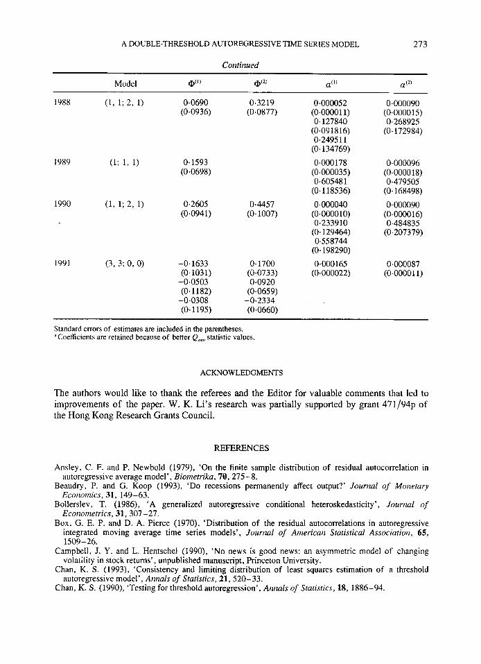
A DOUBLE-THRESHOLD AUTOREGRESSIVE TIME SERIES MODEL 21 3
Continued
1988 (1, 1; 2, 1) 0.0690 (0.0936)
0.1593 (0.0698)
1990 (1, 1; 2, 1) 0.2605 (0.094 1)
1991 ( 3 , 3; 0, 0) -0.1633
-0.0503
-0.0308
(0.1031)
(0.1182)
(0.1 195)
0.3219 (0.0877)
04457 (0.1007)
0.1700 (0.0733) 0.0920
(0.0659) -0.2334 (0.0660)
~~~
0.000052 (0~000011) 0.127840
(0.09 18 16) 0.2495 11
(0.134769) 0.000 178
(0.000035) 0.60548 1
(0.118536) 0.000040
(0~000010) 0.233910
(0- 129464) 0.558744
(0.198290) 0.000 165
(0~000022)
0.000090
0 - 268925 (0- 172984)
(0~000015)
0.000096 (0.0000 18) 0.479505
(0.168498) 0.000090
(0.0000 16) 0-484835
(0-207379)
0.000087 (0-00001 1)
Standard errors of estimates are included in the parentheses. ‘Coefficients are retained because of better Q,,,,,, statistic values.
ACKNOWLEDGMENTS
The authors would like to thank the referees and the Editor for valuable comments that led to improvements of the paper. W. K. Li’s research was partially supported by grant 471/94p of the Hong Kong Research Grants Council.
REFERENCES
Ansley, C. F. and P. Newbold (1979), ‘On the finite sample distribution of residual autocorrelation in autoregressive average model’, Biometrika, 70,275-8.
Beaudry, P. and G. Koop (1993), ‘Do recessions permanently affect output?’ Journal of Monetary Economics, 31, 149-63.
Bollerslev, T. (1986), ‘A generalized autoregressive conditional heteroskedasticity’, Journal of Econornetrics, 31, 307-27.
Box, G. E. P. and D. A. Pierce (1970), ‘Distribution of the residual autocorrelations in autoregressive integrated moving average time series models’, Jourrial of Americaii Statistical Association, 65,
Campbell, J. Y. and L. Hentschel (1990), ‘No news is good news: an asymmetric model of changing
Chan, K. S . (1993), ‘Consistency and limiting distribution of least squares estimation of a threshold
Chan, K. S . (1990), ‘Testing for threshold autoregression’, Annals of Statistics, 18, 1886-94.
1509-26.
volatility in stock returns’, unpublished manuscript, Princeton University.
autoregressive model’, Annals of Statistics, 21, 520-33.
274 C. W. LI AND W. K. LI
Chan, K. S. and H. Tong (1990), ‘On likelihood ratio tests for threshold autoregression’, Journal of Royal
Christie, A. A. (1982), ‘The stochastic behavior of common stock variances’, Journal of Firiancial
Engle, R. F. (1982), ‘Autoregressive conditional heteroskedasticity with estimates of the variance of U.K.
Engle, R. F. and T. Bollerslev (1986), ‘Modeling the persistence of conditional variances’, Eroriornetric
French, K. R., G. W. Schwert and R. K. Stambaugh (1987), ‘Expected stock returns and volatility’,
Hamilton, J. D (1990), ‘Analysis of time series subject to changes in regime’, Jourizal of Econometrics,
Statistical Society, B52,469-76.
Econoinics, 10, 407 -32.
inflation’, Econornetrica, 50, 987- 1008.
Reviews, 5, 1-87.
Journal of Financial Econotnics, 19, 3 -29.
45,39-70. Hinich, M. J. and D. M. Patterson (1985), ‘Evidence of nonlinearity in daily stock return’, Journal of
Business arid Ecorzornic Statistics, 3(1), 69-77. Karpoff, J. M. (1987), ‘The relation between price changes and trading volume: a survey’, Journal of
Quantitative Analysis, 21, No. 11, May, 109- 126. Li, C. W. (1994), On a Double Threshold Autoregressive Heteroskedastic Time Series Model, MPhil
thesis, University of Hong Kong. Li, W. K. (1992), ‘On the asymptotic standard errors of residual autocorrelations in nonlinear time series
modeling’, Biornetrika, 79, 2,435-7. Li, W. K. and K. Lam (1995). ‘Modeling asymmetry in stock returns by a threshold ARCH model’, to
appear in The Statistician. Li, W. K. and T. K. Mak (1994), ‘On the squared residual autocorrelations in conditional heteroskedastic
time series modeling’, Jourrml of Time series Analysis, 15,627 -36. Ljung, G. M. and G. E. P. Box (1978), ‘On a measure of lack of fit in time series models’, Journal of
Applied Probability, 25, 553-64. Mak, T. K. and W. K. Li (1994), ‘Estimation of nonlinear time series with conditional heteroskedastic
variance by iteratively weighted least squares’, unpublished manuscript, Department of Statistics, University of Hong Kong.
Mak, T. K. (1993), ‘Solving nonlinear estimation equations’, Journal of Royal Sratisticd Society, Series
Nelson, D. B. (1990), ‘ARCH models as diffusion approximations’, Journal of Econoinefrics, 45, 7-38. Nelson, D. B. (1991), ‘Conditional heteroskedasticity in asset returns: a new approach’, Ecoriornetrica,
Pesaran, M. H. and S. M. Potter (1994), ‘A floor and ceiling modeling of US output’, Department of Applied Economics Working paper No. 9407, University of Cambridge.
Rabemanjara, R. and J. M. Zakoian (1993), ‘Threshold ARCH model and asymmetries in volatility’, Journal of Applied Econometrics, 8, 3 1-49.
Schwert, G. W. (1989), ‘Why do stock market volatility change over time?’ Jourrial of Finance, 44, 5 , 11 15-53.
Terasvirta, T. and H. M. Anderson (1993), ‘Characterizing nonlinearities in business cycles using smooth transition autoregressive models’ in M. H. Pesaran and S. M. Potter (eds), Noriliriear Dynamics, Chaos arid Econornetrics, 11 1 - 128, Wiley, New York.
Tong, H. (1978), ‘On a threshold model’, in C. H. Chen (ed.), Pattern Recogriiriori arid Sigrid Processing, Sijthoff and Noordhoff, Amsterdam.
Tong, H. and K. S. Lim (1980), ‘Threshold autoregressive, limit cycles and cyclical data’, Journal of the Royal Statistical Society, Series B ,42,245 -92.
Tong, H. (1990), Non-Linear Time Series: A Dynainical System Approach, Oxford University Press, Oxford.
Tsay , R. S. (1989), ‘Testing and modeling threshold autoregressive processes’, Journal of American Statistical Association, 84, 23 1-40.
B, 55, NO. 4,945-55.
59,347-70.
Weiss, A. A. (1986), ‘Asymptotic theory for ARCH models: estimation and testing’, Ecoriornetric Theory, 2, 107-131.