M A X P L A N C K S O C I E T Y

Preprints of theMax Planck Institute for

Research on Collective GoodsBonn 2011/1

Oligopoly as a Socially Embedded Dilemma. An Experiment

Christoph Engel Lilia Zhurakhovska

Preprints of the Max Planck Institute for Research on Collective Goods Bonn 2011/1

Oligopoly as a Socially Embedded Dilemma.An Experiment

Christoph Engel / Lilia Zhurakhovska

January 2011, revised November 2011

Max Planck Institute for Research on Collective Goods, Kurt-Schumacher-Str. 10, D-53113 Bonn http://www.coll.mpg.de

1

Oligopoly as a Socially Embedded Dilemma An Experiment

1. Introduction

Albert Einstein once said: everything should be made as simple as possible – but not simpler.1 Viewed from inside the supply side of the market, competition may be interpreted as a prisoner’s dilemma. In this perspective, collusion is the equivalent of cooperation, competitive behavior is defection. Individually, each supplier is best off if the other suppliers are faithful to the cartel, and she undercuts the collusive price or, for that matter, surpasses her quota. This is certainly a simple way of capturing the essence of the competitors’ dilemma. But is it too simple? Two features of competition are missing in this model: first, the suppliers’ dilemma is embedded in a market, and in society at large. If they cooperate, suppliers impose a distributional loss on the demand side, and they generate a deadweight loss, to the detriment of society. Second, both on efficiency and on distributional grounds, in almost all legal orders of the world, the law steps in and combats cartels (for an overview, see Hylton and Deng 2007). In a pure world of profit maximization, suppliers have no reticence to inflict harm on the opposite side of the market. And illegality is not an argument per se. Risk-neutral suppliers only react if apprehension and enforcement are sufficiently likely, and if the sanction is sufficiently severe. Of course, in repeated or nested interaction, it may be profit-maximizing to play by the rules. But behaviorally, this explanation is incomplete. On the one hand, the rich experimental literature on oligopoly demonstrates that subjects frequently overcome the competition dilemma (see Engel 2007 for a meta-study). Apparently, the Nash equilibrium of the stage game is not the exclusive force driving the decision to collude. This is in line with a rich experimental literature on prisoner dilemma games. In such games, cooperation is much more pronounced than models of perfectly anticipatory, profit-maximizing agents predict. To a remarkable degree, experimental subjects are willing to go the risk of being exploited (see already Rapoport and Chammah 1965). If the prisoner’s dilemma model captures the essence of the decision to collude, from a behavioral perspective a much higher degree of collusion is to be expected. On the other hand, it is an established piece of wisdom in the experimental community that there is more cooperation in a public good than in an oligopoly, although structurally both are prisoner’s dilemma games (Ledyard 1995; Zelmer 2003; Chaudhuri 2011: survey the evidence). Specifically, in a behavioral perspective the two features that distinguish oligopoly from a naked prisoner’s dilemma can be expected to dampen cooperation. Inequity-averse oligopolists might also be averse to

1 As quoted by Roger Sessions, New York Times, 8 January 1950.

2

impose harm on an innocent outsider. Risk-averse or loss-averse oligopolists might dread sanctions, even beyond their expected payoff. In this paper, we experimentally test these two reasons, both separately and jointly, why a cartel might not just be an ordinary prisoner’s dilemma. In order to avoid framing effects and to prevent participants from activating their world knowledge about the effects and the desirability of cartels, we test them on a standard matrix game with neutral framing. Our baseline is a one-shot symmetric two-person prisoner’s dilemma. In our treatments, using the strategy method (Selten 1967), we expose two active players to increasing levels of harm on an outsider if they do not both defect (meant to capture the effect on the opposite market side); we expose them to an increasing risk of not receiving gains from cooperation (meant to capture the risk of sanctions); and we cross both effects. It turns out that, compared with the naked prisoner’s dilemma (baseline), sanctions only slightly decrease cooperation, while negative externalities even slightly enhance it. Obviously neither legal interventions (sanctions) nor moral norms (negative externalities) lead to more desirable behavior from the perspective of the society as a whole. This is remarkable. In our experiment, participants have no hesitance to impose harm on passive, innocent outsiders. And turning gains from cooperation into a lottery only has a very small effect, compared with getting the certainty equivalent with certainty. Seemingly, from a behavioral perspective one does not miss anything important if one analyses competition as a simple dilemma of insiders. The fact that competition is embedded in a market, and in a society that cares about market outcomes, has hardly any effect on the behavior of market participants. The gloomy picture of supplier callousness is supported by a series of post-experimental tests. We measure the individual willingness to harm outsiders by a dictator game variant. It turns out that behavior in this post-experimental test does not significantly explain choices in the prisoner’s dilemma with externalities. Likewise, from a behavioral perspective, one might have expected that participants shy away from cooperation in a prisoner’s dilemma with uncertain gains the more they are risk-averse. We measure risk preferences by a standard test (Holt and Laury 2002). This does not explain choices in the prisoner’s dilemma with uncertain gains from cooperation either. If participants take gains from collusion as the reference point, one would have expected them to shy away from cooperation the more they are loss-averse. To test this explanation, we also measure the individual degree of loss aversion, using the test proposed by (Gächter, Johnson et al. 2007). Again, we do not find significant results. Yet we get a more nuanced, and an even less comforting, picture once we control for individual beliefs about the willingness of others to cooperate. This control variable has a strong and significant effect throughout.

3

Conditional on beliefs, we find significant treatment differences. If we control for the individual level of optimism about cooperativeness, the fact matters that the oligopoly dilemma is socially embedded. Knowing that they have to impose harm on outsiders has a striking effect. On the one hand, players become more pessimistic. Yet conditional on beliefs, when cooperation with the other active players imposes harm on an outsider, players cooperate more, irrespective of the degree of harm. Knowing that the opposite market side suffers not only fails to induce greater caution; it even seems to help firms coordinate. We find a similar effect if participants not only impose harm on an outsider but, additionally, face a sanction. By contrast, conditional on beliefs, sanctions basically only matter if cooperation no longer pays in expected payoff. From a policy perspective, these are troubling findings. Of course, industrial organization scholars always had second thoughts when analyzing competition as a stage game of profit-maximizing actors. The prediction of the Bertrand model (with homogenous goods) seemed too good to be true (see, e.g., the discussion in Tirole 1988: chapter 5). They were skeptical that the mere structure of the game would suffice to deter collusion. Yet our experiment was motivated by the hope that, at least, the fact that the suppliers’ dilemma is embedded in a market and in a legal order would mitigate the otherwise pronounced ability to overcome the dilemma. As our results show, this hope is not well founded. Antitrust has reason to dread the willingness of suppliers to incur the risk of cooperation. The fact that the opposite market side suffers if collusion succeeds even helps suppliers coordinate. The remainder of the paper is organized as follows: Section 2 relates the paper to the existing literature. Section 3 introduces the design. Section 4 makes theoretical predictions. Section 5 presents and discusses the treatment effects. Section 6 exploits the post-experimental tests to generate explanations for these effects. Section 7 concludes.

2. Related Literature

There is a rich experimental literature on oligopoly (see the meta-study by Engel 2007); yet it does not focus on the fact that oligopoly is socially and legally embedded. The effects of externalities on passive outsiders have only rarely been studied. To the best of our knowledge, they have not been tested in a standard prisoner’s dilemma. Güth and van Damme (1998) present an ultimatum game with an externality on an inactive third player who has no say. The proposer decides how to divide the pie between three players. The division is executed if and only if the responder accepts. Otherwise, all three players receive nothing. In this game, the outsider receives very little. If the responder only learns the fraction the proposer wants to give the outsider, proposers keep almost everything for themselves. In anticipation, responders are very likely to reject the (mostly unknown) offer. Bolton and Ockenfels (2010) study

4

lottery choice tasks in which the actor’s choice also influences the payoff of a non-acting second player. This induces participants to take larger risks, provided the safe option yields unequal payoffs. Abbink (2005) plays a two-person bribery game in which corruption negatively affects passive workers. He concludes that reciprocity between briber and official overrules concerns about distributive fairness towards other members of the society. Ellman and Pezanis-Christou (2010) study how a firm’s organizational structure influences ethical behavior towards passive outsiders. A firm of two players decides on its production strategy, which influences a passive third player. They find that horizontally organized firms in which the firm’s decision corresponds to the average of both individual decisions are less likely to harm the outsider than consensus-based firms or firms in which one of both members is the boss. Uncertainty has been introduced into prisoner’s dilemma games the following way: Kahn and Murnighan (1993) expose participants in a two-person prisoner’s dilemma to uncertainty about their counterpart’s payoff, which leads to less cooperation, and they explore the interaction with payoff asymmetry. Our design differs in that there is also uncertainty about one’s own payoff. Bereby-Meyer and Roth (2006) compare a prisoner’s dilemma where all payoffs are certain with one where all are lottery tickets. The latter decreases cooperation in repeated interaction, but increases cooperation if partners change every period. Our design differs in that we introduce uncertainty only for the case of joint cooperation, while all other payoffs are certain (since they involve no risk of antitrust intervention). Kunreuther, Silvasi et al. (2009) manipulate the payoffs if at least one player does not cooperate. In the stochastic setting, players then run the risk of a loss. Hence gains from cooperation consist of perfect insurance. This induces less cooperation than a standard deterministic game, where all payoffs are certain. In a way, in one of our treatments, we are studying the mirror situation, where uncertainty is present only if both players cooperate. Grechenig, Nicklisch et al. (2010) manipulate the quality of the information other contributors receive in a linear public good with a punishment option. They find that contributions are not significantly different from the case of perfect feedback if the information is almost always correct. By contrast, if feedback is noisier, the beneficial effect of punishment vanishes. In our game, the sanction itself is uncertain. It is inflicted by design, not by the decision of a sanctioning authority. Sabater-Grande and Georgantzis (2002) measure the level of risk aversion of individual participants, and later expose them to a repeated prisoner’s dilemma. The more participants are risk-averse, the more they are likely to defect. However, highly risk-averse participants are also more sensitive to signals by their partners when the discounting of earnings in future periods is uncertain. Our experiment differs in that we have a one-shot game, and we manipulate the degree of uncertainty, and the level of harm imposed on an outsider. Blanco, Engelmann et al. (2011) have

5

participants, among other games, play a dictator and a prisoner’s dilemma game. They find that the degree of aversion against advantageous inequity derived from the dictator game does not explain choices in the prisoner’s dilemma at an individual level. We have a different research question, and we also elicit beliefs, which turns out crucial for explaining behavior in the prisoner’s dilemma.

3. Design

We have four treatments: a Baseline with neither externalities nor sanctions; a treatment with only negative Externalities; a treatment with only Sanctions; finally a treatment combining Externalities+Sanctions. We deliberately avoid a market frame. This not only makes sure that our results are not driven by the frame. It is also necessary to disentangle the effects of externalities and sanctions. In a market setting, from their world knowledge subjects would know that collusion has a detrimental effect on the opposite market side, and that collusion is illegal.

a) Baseline

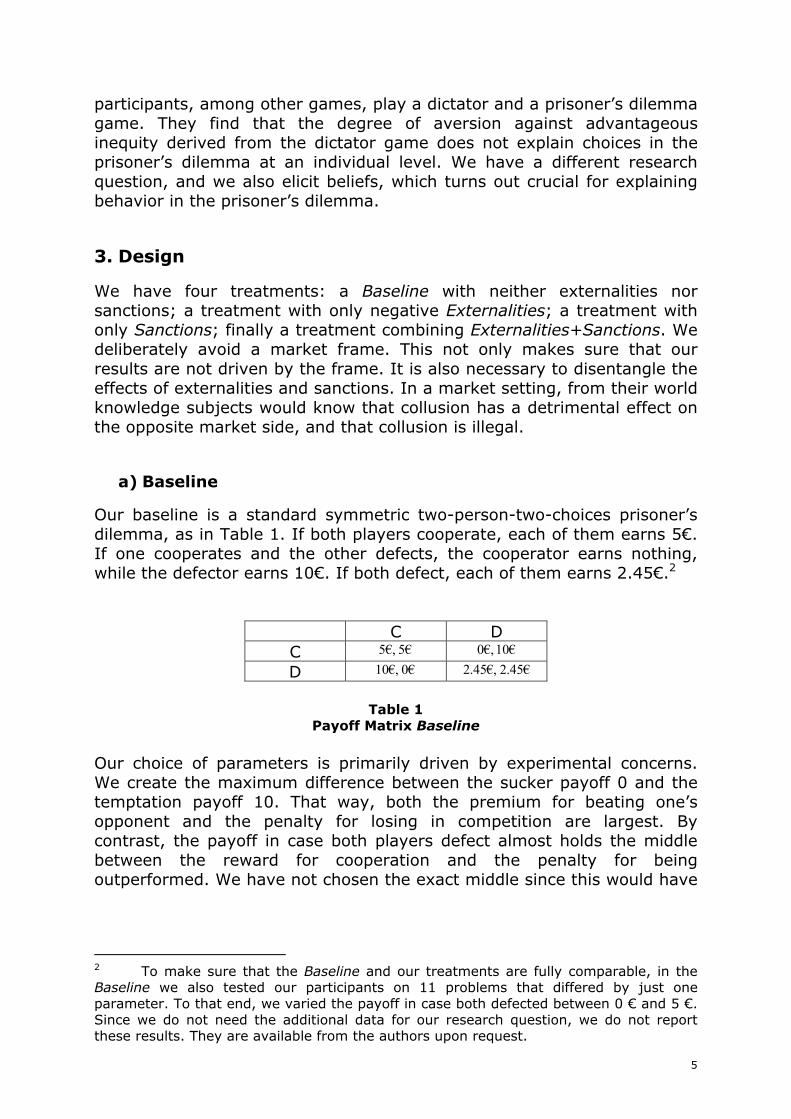
Our baseline is a standard symmetric two-person-two-choices prisoner’s dilemma, as in Table 1. If both players cooperate, each of them earns 5€. If one cooperates and the other defects, the cooperator earns nothing, while the defector earns 10€. If both defect, each of them earns 2.45€.2

C D C €5€,5 €10€,0

D €0€,10 €45.2€,45.2

Table 1

Payoff Matrix Baseline Our choice of parameters is primarily driven by experimental concerns. We create the maximum difference between the sucker payoff 0 and the temptation payoff 10. That way, both the premium for beating one’s opponent and the penalty for losing in competition are largest. By contrast, the payoff in case both players defect almost holds the middle between the reward for cooperation and the penalty for being outperformed. We have not chosen the exact middle since this would have

2 To make sure that the Baseline and our treatments are fully comparable, in the Baseline we also tested our participants on 11 problems that differed by just one parameter. To that end, we varied the payoff in case both defected between 0 € and 5 €. Since we do not need the additional data for our research question, we do not report these results. They are available from the authors upon request.

6

created an identification problem in the Sanctions treatment.3 For this payoff, we deliberately have not chosen either extreme. If participants earn 0€ in case both defect, cooperation is no longer strictly dominated. Strictly speaking, the game is no longer a prisoner’s dilemma. At the opposite extreme, the equilibrium is not affected. But if participants earn 5€ in case both defect, gains from cooperation are 0. The situation is no longer a dilemma. In a stylized way, our game captures a one-shot Bertrand market with constant marginal cost where two firms individually decide whether to set the collusive price (C) or to engage in a price war (D). If both engage in (tacit or explicit) collusion, both set the monopoly price and split the monopoly profit evenly. If only one of them starts a price war, it undercuts the collusive price by the smallest possible decrement. As is standard in the theoretical literature, we assume this decrement to be infinitesimally small, which implies that the aggressive firm cashes in the entire monopoly profit, while the firm that is faithful to the cartel receives nothing. If both firms start fighting, they end up in the Nash equilibrium. The positive payoff in the case of joint defection requires a slightly richer model, for instance one with heterogeneous products.4 In a repeated game, the effects of optimism, generosity, risk, and loss aversion would be overshadowed by reputation effects. We therefore test our subjects on a one-shot game. That way, we also need not be concerned that players might take turns. There is no room for an equilibrium in iterations.

b) Externalities

In the Externalities treatment, payoffs for the active players are as in the Baseline. Yet in this treatment, each group consists of three players. If at least one of the two active players cooperates, a third, inactive player suffers harm €h . In a stylized way, this player captures the detrimental effects cooperating firms impose on the opposite market side, and on society at large. Using the strategy method (Selten 1967), we vary

3 In Sanctions, gains from cooperation are only received with probability p . Had we set the payoff in the case of joint defection at exactly €5.2 , with 5.=p , the expected payoff of joint defection would have been exactly the same as the expected payoff of joint cooperation. We could not have said whether participants are overdeterred if, with

5.=p , they choose to defect. 4 For sure, in a Bertrand market with heterogeneous products, undercutting does not allow a firm to reap the entire monopoly profit. The opponent still makes a small, but positive profit. We might have captured this by a payoff of €9 if a firm defects while the other cooperates, and by a payoff of €1 in case the other firm defects while this firm stays faithful to the cartel. We have chosen not to do so for the sake of giving our participants a design that is a as simple and transparent as possible.

7

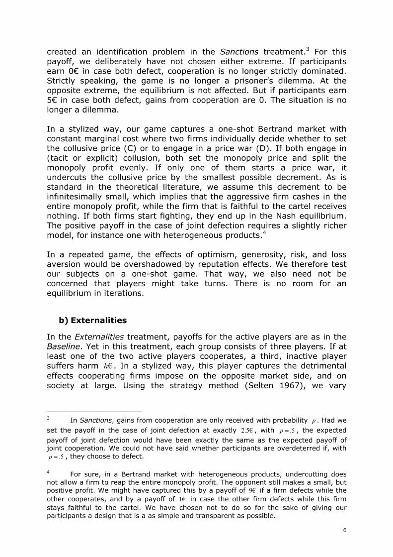
€]3.9€,3[.∈h , in 11 equal steps of .9€. This makes for the following payoff matrix:

C D C €€5€5 h−,, €€10€,0 h−,

D €€€10 h−,0, €0€,45.2€,45.2

Table 2

Payoff Matrix Externalities This manipulation is meant to capture the loss in consumer welfare inherent in anticompetitive behavior. As in the field, this harm is not confined to the case of successful collusion. It also results if one firm sets the collusive price or quantity, while the other infinitesimally undercuts. Therefore in the experiment we do not confine harm to the situation where both active players cooperate. We impose the same harm if one cooperates while the other defects. We normalize harm to zero if both active players defect. Factor h thus captures the additional harm resulting from anticompetitive behavior.

c) Sanctions

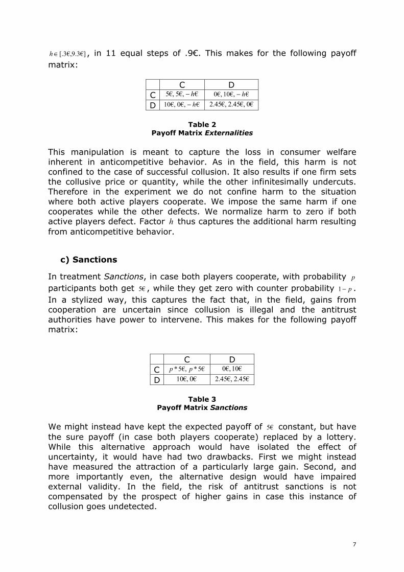
In treatment Sanctions, in case both players cooperate, with probability p participants both get €5 , while they get zero with counter probability p−1 . In a stylized way, this captures the fact that, in the field, gains from cooperation are uncertain since collusion is illegal and the antitrust authorities have power to intervene. This makes for the following payoff matrix:

C D C €5*€5* pp , €10€,0

D €€10 0, €45.2€,45.2

Table 3

Payoff Matrix Sanctions We might instead have kept the expected payoff of €5 constant, but have the sure payoff (in case both players cooperate) replaced by a lottery. While this alternative approach would have isolated the effect of uncertainty, it would have had two drawbacks. First we might instead have measured the attraction of a particularly large gain. Second, and more importantly even, the alternative design would have impaired external validity. In the field, the risk of antitrust sanctions is not compensated by the prospect of higher gains in case this instance of collusion goes undetected.

8

At the end of the game, after the computer has paired participants and chosen the payoff-relevant game, in a further random draw it decides whether gains from cooperation materialize, with the determined probability. Again using the strategy method, we vary ]9,.1[.∈p , in eleven equal steps of .08. Hence we exclude the situations where getting gains from cooperation is certain (since this would be the same as the Baseline), and where not getting gains from cooperation is certain (since this would make the game trivial). To avoid any demand effect, we frame the game neutrally and do not speak of sanctions. All we do is to turn gains from cooperation into a lottery.

Note that, with 49.<p , the expected payoff of joint cooperation is smaller than the expected payoff of joint defection. Consequently, risk-neutral actors will not choose cooperation, even if they believe all other participants are willing to cooperate, and if they are not willing to exploit their random counterpart. We choose this array of parameters for two reasons. In line with (Becker 1968), we wonder whether participants might be overly attracted by the prospect of a large gain, i.e., the difference between 5€ and the sure 2.45€. Also, in the final Externalities+Sanctions treatment that crosses the effects from the Externalities and the Sanctions treatments, we want to keep the same parameters, and we want more scope for disentangling motives. In antitrust, collusion is straightforwardly forbidden and sanctioned. By contrast, undercutting (even if only by a small amount) is not at variance with antitrust. On the contrary, it is the behavior antitrust desires. In most legal orders, holding a dominant position is not illegal either (see the overview by Hylton and Deng 2007). Legal orders are divided over acts that help a firm acquire or defend a dominant position. Only the abuse of dominance is illegal in most legal orders. Yet it requires more than setting an infracollusive price. In keeping with this, we confine the uncertainty (parameter p ) to the case where both participants cooperate, while the defector gets 10€ with certainty if the other player cooperates.

d) Externalities + Sanctions

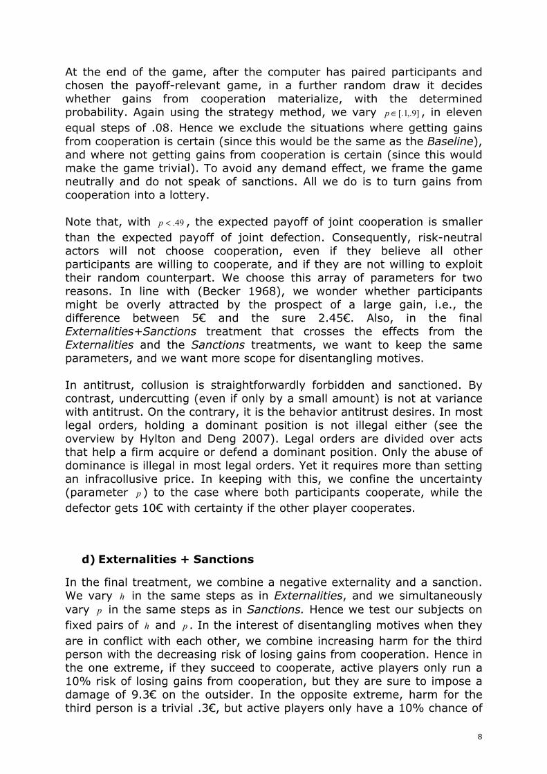
In the final treatment, we combine a negative externality and a sanction. We vary h in the same steps as in Externalities, and we simultaneously vary p in the same steps as in Sanctions. Hence we test our subjects on fixed pairs of h and p . In the interest of disentangling motives when they are in conflict with each other, we combine increasing harm for the third person with the decreasing risk of losing gains from cooperation. Hence in the one extreme, if they succeed to cooperate, active players only run a 10% risk of losing gains from cooperation, but they are sure to impose a damage of 9.3€ on the outsider. In the opposite extreme, harm for the third person is a trivial .3€, but active players only have a 10% chance of

9

actually getting gains from cooperation. Our way of crossing levels of harm with levels of risk is also meant to capture the fact that, in the field, the less firms are likely to be detected, the more they are likely to impose harm on the opposite market side, and vice versa. In this game, the payoff matrix looks as follows:

C D C €€5*€5* hpp −,, €€10€,0 h−,

D €€€10 h−,0, €0€,45.2€,45.2

Table 4

Payoff Matrix Externalities + Sanctions

e) Procedures

The experiment was run at the University of Bonn in May 2010 with a computerized interaction using z-Tree (Fischbacher 2007). ORSEE (Greiner 2004) was used to invite subjects from a subject pool of approximately 3500 subjects. Each subject played in one of the four treatments and no subject played in more than one. We collected 48 independent observations in all treatments; in treatments Externalities and Externalities+Sanctions, we also invited 24 inactive players, randomly assigned to be the potential targets of externalities. We thus have a total of 192 independent observations. Subjects were on average 24.04 years old (range 17-50). 58.33% were female. They held various majors.5 Each session lasted about one and a half hours. There was no show-up fee, but participants were guaranteed a minimum payoff of 5€.6 Subjects earned on average 10.91€ (equivalent to 13.66$ on the last day of the experiment, range 5€-25.85€). In the Baseline, they earned on average 9.84€; in Externalities, the average sum was 11.80€, in Sanctions, it was 10.96€, and in Externalities+Sanctions, it was 10.71€. These earnings partly stem from post-experimental tests, which we report below.

4. Predictions

Since our game is a one-shot prisoner’s dilemma, money-maximizing agents defect in the Baseline. Empirically, many experimental subjects have been found to be conditional cooperators (Fischbacher, Gächter et al. 2001; Fischbacher and Gächter 2010). Pure conditional cooperators (at least weakly) prefer cooperation over defection if they expect their counterpart to cooperate with certainty. This implies that they resist the temptation to exploit their

5 22.08% lawyers, 13.75% economists. 6 This applied to participants who had a total of less than 5€ from the main experiment and all post-experimental tests, especially if they made losses.

10

counterpart. If conditional cooperators are perfectly optimistic, they do not expect to run a risk. Consequently, in the Baseline, perfectly optimistic conditional cooperators cooperate. In line with previous experiments, we expect conditional cooperation to be more prevalent than outright selfishness. Yet we expect participants to be less than perfectly optimistic. If their beliefs make them less optimistic, conditional cooperators run the risk of not getting gains from cooperation. If they are neutral to risk and losses, they compare the expected payoff of cooperation with the expected payoff of defection. If they are pure conditional cooperators in the sense of not desiring gains from exploitation, they discount gains from cooperation by their subjective degree of pessimism, and compare them with the minimum payoff in case they defect. Hence for such actors, the size of this outside option matters. Cooperation is the less likely, the smaller the difference is between the outside option and gains from cooperation. Cooperation becomes even less likely if an actor is an imperfect conditional cooperator, meaning that she strives to outperform her counterpart, if only slightly (Fischbacher and Gächter 2010); if she is averse against the risk of not getting gains from cooperation since her counterpart defects; if she dreads losing the outside option since she is exploited by her counterpart (Tversky and Kahneman 1992). If these personality traits combine, the dampening effect on cooperation multiplies. If this actor defects while the other actor cooperates, two effects combine. Payoffs are unequal, with an advantage for the defecting actor (as modelled in Fehr and Schmidt 1999; Bolton and Ockenfels 2000). If the first actor expects the second to cooperate, she also violates the second actor’s expectation of reciprocal action (as modelled in Rabin 1993; Dufwenberg and Kirchsteiger 2004). The reciprocity motive is not affected by adding a third player in treatment Externalities. Since the third player is inactive, she has no chance to reciprocate kind or unkind behavior. By contrast, in Externalities the inequity balance is more complicated. If both active players defect, they are symmetrically favored with respect to the inactive player. If both cooperate, they are favored even more. If one defects while the other cooperates, the defecting one is strongly favored in comparison with both other players, while the cooperating one has a payoff of 0€, and the inactive player incurs a loss of –h€. This line of argument, however, neglects that in case both active players defect, the payoff difference in comparison with the inactive players “is not their fault”. Actually if they want to be kind to the inactive player, defecting is the best thing both can do. In situations that are structurally similar to the one tested here, it has been shown that intentions matter in the assessment of fairness (Falk, Fehr et al. 2008). Taking this into account, the Externalities treatment exposes active players to a conflict

11

between fairness with the inactive player (calling for both defecting) and the motives behind conditional cooperation (calling for cooperation, provided the player is sufficiently optimistic about cooperativeness in this population). However, defection has a double dividend in this game: the defecting active player for herself at least secures the payoff she expects if both players defect cell, and she does the best she can to protect the inactive player from harm. The effect should be the stronger the more severe the harm on the outsider is. We therefore predict

H1: In Externalities, there is less cooperation than in the Baseline.

In Sanctions, gains from cooperation are uncertain. If the expected payoff of these gains is below the certain value of the outside option, even perfectly optimistic, risk-neutral conditional cooperators should defect. Even above this threshold, the more participants are risk-averse, the less cooperation we should see. If participants take gains from cooperation to be the reference point, they should also consider not getting these gains as a loss. This leads to

H2: In Sanctions, there is no cooperation if the expected payoff of gains from cooperation is below the outside payoff. There is less cooperation than in the Baseline.

Both in Externalities and in Sanctions, we expect less cooperation than in the Baseline. In Externalities+Sanctions, we have chosen parameters such that severe harm goes together with a small risk of losing gains from cooperation, and vice versa. We therefore have no reason for considering whether both effects might neutralize each other. We predict less cooperation than in the Baseline. We have no theoretical reasons to expect the effect of harm on outsiders to be substantially bigger than the effect of a risk of losing the cooperative gain. We therefore predict

H3: In Externalities+Sanctions, there is less cooperation than in the Baseline.

5. Treatment Effects

a) Baseline

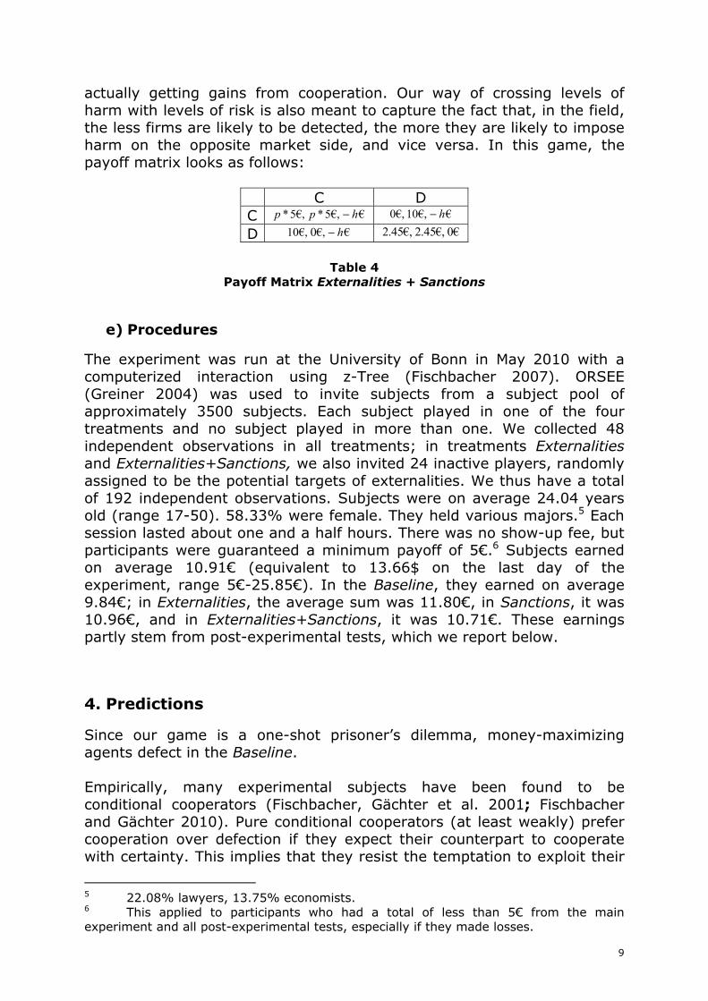
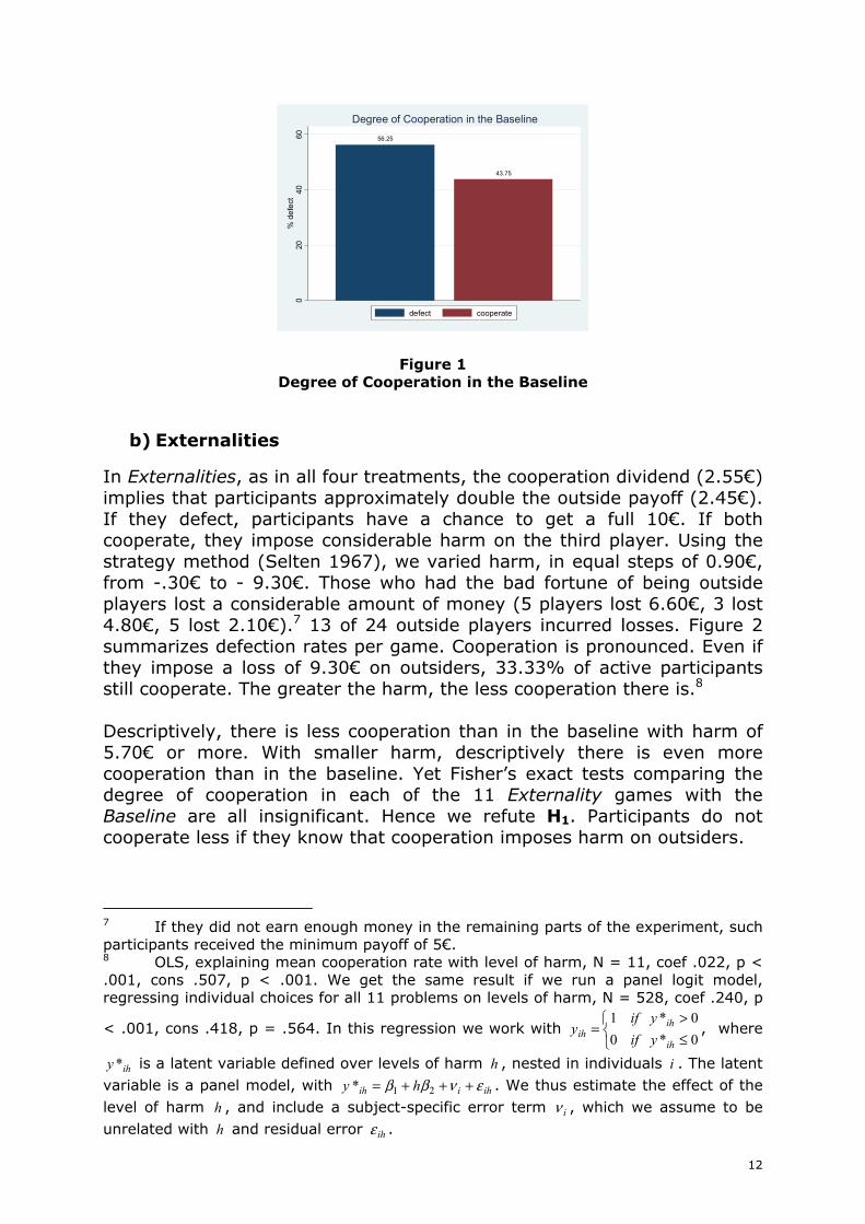
The Baseline exposes participants to a standard prisoner’s dilemma. The purpose of the baseline is to provide us with a benchmark. While the majority defected, 43.75% of our participants were willing to take the risk of cooperation.

12

56.25

43.75

020

4060

% d

efe

ct

Degree of Cooperation in the Baseline

defect cooperate

Figure 1 Degree of Cooperation in the Baseline

b) Externalities

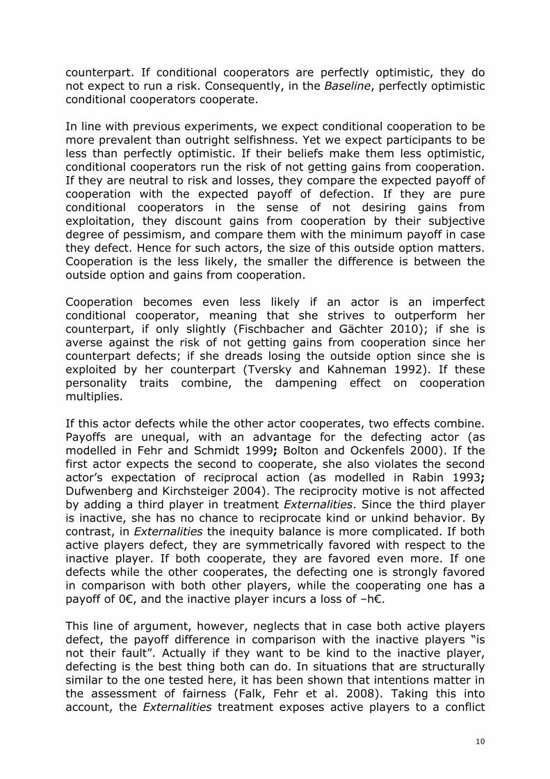
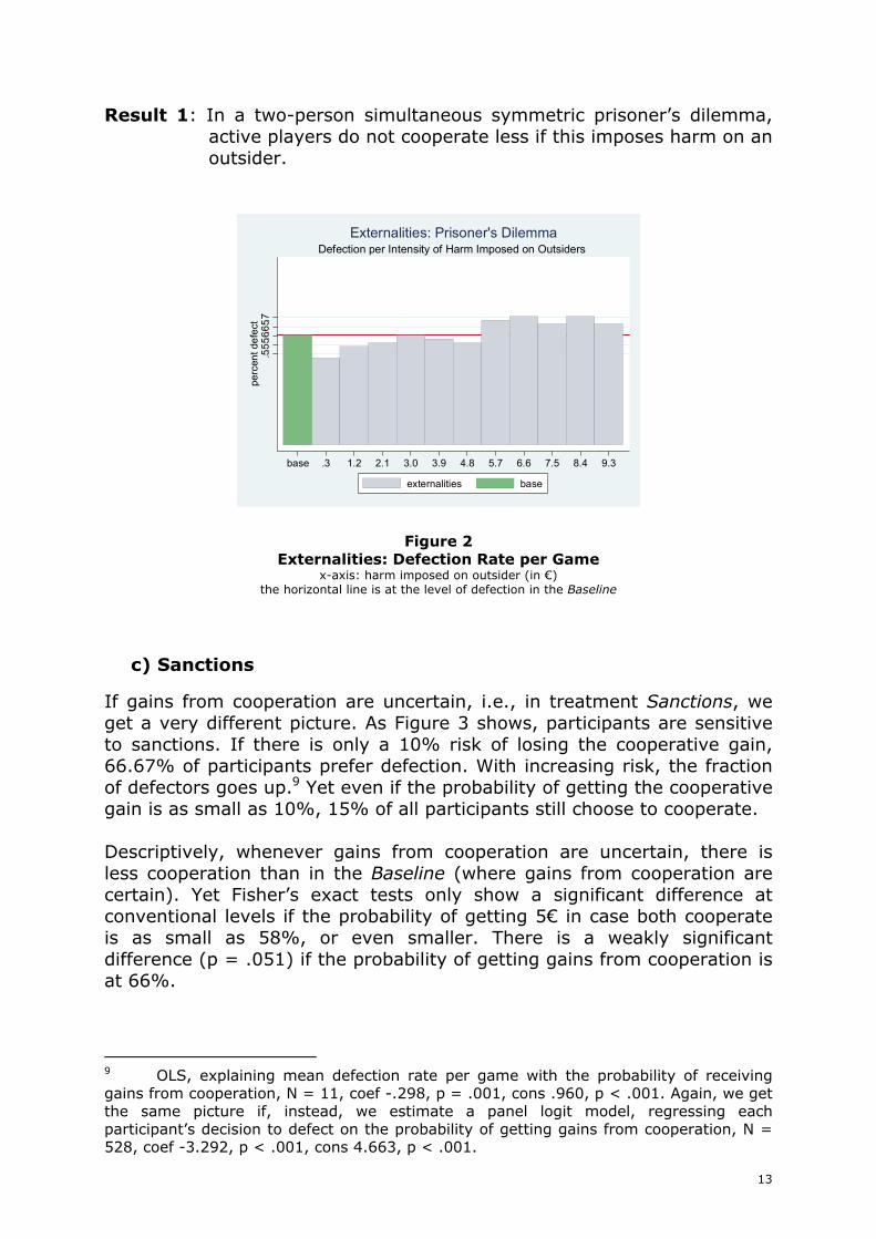
In Externalities, as in all four treatments, the cooperation dividend (2.55€) implies that participants approximately double the outside payoff (2.45€). If they defect, participants have a chance to get a full 10€. If both cooperate, they impose considerable harm on the third player. Using the strategy method (Selten 1967), we varied harm, in equal steps of 0.90€, from -.30€ to - 9.30€. Those who had the bad fortune of being outside players lost a considerable amount of money (5 players lost 6.60€, 3 lost 4.80€, 5 lost 2.10€).7 13 of 24 outside players incurred losses. Figure 2 summarizes defection rates per game. Cooperation is pronounced. Even if they impose a loss of 9.30€ on outsiders, 33.33% of active participants still cooperate. The greater the harm, the less cooperation there is.8 Descriptively, there is less cooperation than in the baseline with harm of 5.70€ or more. With smaller harm, descriptively there is even more cooperation than in the baseline. Yet Fisher’s exact tests comparing the degree of cooperation in each of the 11 Externality games with the Baseline are all insignificant. Hence we refute H1. Participants do not cooperate less if they know that cooperation imposes harm on outsiders.

7 If they did not earn enough money in the remaining parts of the experiment, such participants received the minimum payoff of 5€. 8 OLS, explaining mean cooperation rate with level of harm, N = 11, coef .022, p < .001, cons .507, p < .001. We get the same result if we run a panel logit model, regressing individual choices for all 11 problems on levels of harm, N = 528, coef .240, p

< .001, cons .418, p = .564. In this regression we work with

≤>

=0*00*1

ih

ihih yif

yify , where

ihy* is a latent variable defined over levels of harm h , nested in individuals i . The latent variable is a panel model, with ihiih hy ενββ +++= 21* . We thus estimate the effect of the level of harm h , and include a subject-specific error term iν , which we assume to be unrelated with h and residual error ihε .

13

Result 1: In a two-person simultaneous symmetric prisoner’s dilemma, active players do not cooperate less if this imposes harm on an outsider.

.5.5

5.6.

65.

7pe

rcen

t de

fect

base .3 1.2 2.1 3.0 3.9 4.8 5.7 6.6 7.5 8.4 9.3

externalities base

Defection per Intensity of Harm Imposed on OutsidersExternalities: Prisoner's Dilemma

Figure 2 Externalities: Defection Rate per Game

x-axis: harm imposed on outsider (in €) the horizontal line is at the level of defection in the Baseline

c) Sanctions

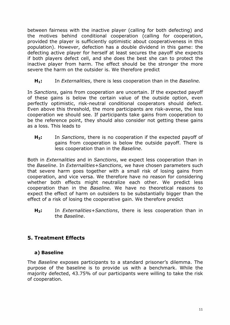
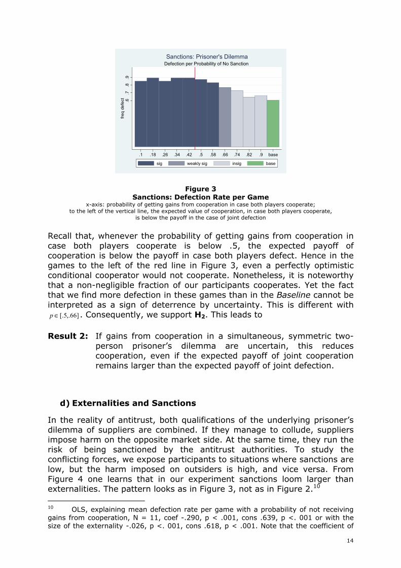
If gains from cooperation are uncertain, i.e., in treatment Sanctions, we get a very different picture. As Figure 3 shows, participants are sensitive to sanctions. If there is only a 10% risk of losing the cooperative gain, 66.67% of participants prefer defection. With increasing risk, the fraction of defectors goes up.9 Yet even if the probability of getting the cooperative gain is as small as 10%, 15% of all participants still choose to cooperate. Descriptively, whenever gains from cooperation are uncertain, there is less cooperation than in the Baseline (where gains from cooperation are certain). Yet Fisher’s exact tests only show a significant difference at conventional levels if the probability of getting 5€ in case both cooperate is as small as 58%, or even smaller. There is a weakly significant difference (p = .051) if the probability of getting gains from cooperation is at 66%.

9 OLS, explaining mean defection rate per game with the probability of receiving gains from cooperation, N = 11, coef -.298, p = .001, cons .960, p < .001. Again, we get the same picture if, instead, we estimate a panel logit model, regressing each participant’s decision to defect on the probability of getting gains from cooperation, N = 528, coef -3.292, p < .001, cons 4.663, p < .001.

14

.6.7

.8.9

fre

q de

fect

.1 .18 .26 .34 .42 .5 .58 .66 .74 .82 .9 base

sig weakly sig insig base

Defection per Probability of No SanctionSanctions: Prisoner's Dilemma

Figure 3 Sanctions: Defection Rate per Game

x-axis: probability of getting gains from cooperation in case both players cooperate; to the left of the vertical line, the expected value of cooperation, in case both players cooperate,

is below the payoff in the case of joint defection

Recall that, whenever the probability of getting gains from cooperation in case both players cooperate is below .5, the expected payoff of cooperation is below the payoff in case both players defect. Hence in the games to the left of the red line in Figure 3, even a perfectly optimistic conditional cooperator would not cooperate. Nonetheless, it is noteworthy that a non-negligible fraction of our participants cooperates. Yet the fact that we find more defection in these games than in the Baseline cannot be interpreted as a sign of deterrence by uncertainty. This is different with

]66,.5[.∈p . Consequently, we support H2. This leads to Result 2: If gains from cooperation in a simultaneous, symmetric two-

person prisoner’s dilemma are uncertain, this reduces cooperation, even if the expected payoff of joint cooperation remains larger than the expected payoff of joint defection.

d) Externalities and Sanctions

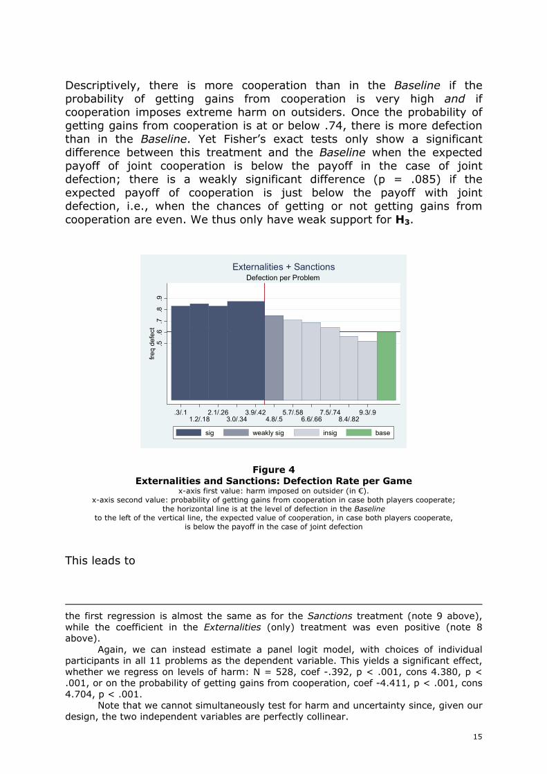
In the reality of antitrust, both qualifications of the underlying prisoner’s dilemma of suppliers are combined. If they manage to collude, suppliers impose harm on the opposite market side. At the same time, they run the risk of being sanctioned by the antitrust authorities. To study the conflicting forces, we expose participants to situations where sanctions are low, but the harm imposed on outsiders is high, and vice versa. From Figure 4 one learns that in our experiment sanctions loom larger than externalities. The pattern looks as in Figure 3, not as in Figure 2.10 10 OLS, explaining mean defection rate per game with a probability of not receiving gains from cooperation, N = 11, coef -.290, p < .001, cons .639, p <. 001 or with the size of the externality -.026, p <. 001, cons .618, p < .001. Note that the coefficient of

15

Descriptively, there is more cooperation than in the Baseline if the probability of getting gains from cooperation is very high and if cooperation imposes extreme harm on outsiders. Once the probability of getting gains from cooperation is at or below .74, there is more defection than in the Baseline. Yet Fisher’s exact tests only show a significant difference between this treatment and the Baseline when the expected payoff of joint cooperation is below the payoff in the case of joint defection; there is a weakly significant difference (p = .085) if the expected payoff of cooperation is just below the payoff with joint defection, i.e., when the chances of getting or not getting gains from cooperation are even. We thus only have weak support for H3.

.5.6

.7.8

.9fr

eq

defe

ct

.3/.11.2/.18

2.1/.263.0/.34

3.9/.424.8/.5

5.7/.586.6/.66

7.5/.748.4/.82

9.3/.9

sig weakly sig insig base

Defection per ProblemExternalities + Sanctions

Figure 4 Externalities and Sanctions: Defection Rate per Game

x-axis first value: harm imposed on outsider (in €). x-axis second value: probability of getting gains from cooperation in case both players cooperate;

the horizontal line is at the level of defection in the Baseline to the left of the vertical line, the expected value of cooperation, in case both players cooperate,

is below the payoff in the case of joint defection

This leads to

the first regression is almost the same as for the Sanctions treatment (note 9 above), while the coefficient in the Externalities (only) treatment was even positive (note 8 above).

Again, we can instead estimate a panel logit model, with choices of individual participants in all 11 problems as the dependent variable. This yields a significant effect, whether we regress on levels of harm: N = 528, coef -.392, p < .001, cons 4.380, p < .001, or on the probability of getting gains from cooperation, coef -4.411, p < .001, cons 4.704, p < .001.

Note that we cannot simultaneously test for harm and uncertainty since, given our design, the two independent variables are perfectly collinear.

16

Result 3: Even if gains from cooperation are mildly uncertain, knowing that they impose severe harm on an outsider does not induce active players in a simultaneous two-person prisoner’s dilemma to cooperate less.

6. Potential and Actual Driving Forces

In hypothesis H1, we had expected that there would be less cooperation in Externalities since players might be reticent to impose harm on innocent outsiders. In hypothesis H2, we had expected that there would be less cooperation in Sanctions, since participants are risk-averse or loss-averse. We have not found a significant difference between the Baseline and Externalities, and the difference between the Baseline and Sanctions is not very pronounced. Using post-experimental tests, we now test whether the expected driving forces have had an effect.

a) Reticence to Impose Harm

To test whether the reticence to impose harm explains choices in a prisoner’s dilemma with outsiders, after they have played the prisoner’s dilemma, we tested our participants on a variant of the dictator game. We asked our subjects to choose between two situations: in situation 1, the proposer and her partner both got 5€. In situation 2, the proposer had a chance of 10 ≤≤ a to get 10€, and a chance of a−1 to get 5€, while the partner got nothing. The rules of the game were common knowledge. Again using the strategy method (Selten 1967), we varied ]1,0[∈a , in equal steps of .1. We asked participants to make their choices for each of the 11 games. All participants made a choice in the role of the dictator, with random draws defining roles and matching participants, after the experiment. All problems are presented simultaneously on one computer screen. At the end of the experiment, one situation is chosen at random, and another random draw determines whether dictators make the high profit, provided they have chosen the lottery. We only give feedback after the entire experiment is over. The game is as follows:

Situation 1 €5€,5

Situation 2 €0€,5*)1(€10* aa −+

Table 5

Payoff Matrix Dictator Game Variant left payoff is for dictator, right payoff is for recipient

We have our subjects choose between a lottery and a safe outcome, rather than between two safe outcomes, to maintain an element of risk. Both in the prisoner’s dilemma and in this game, a player can make sure

17

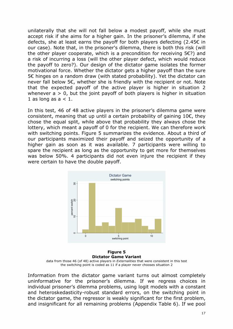
unilaterally that she will not fall below a modest payoff, while she must accept risk if she aims for a higher gain. In the prisoner’s dilemma, if she defects, she at least earns the payoff for both players defecting (2.45€ in our case). Note that, in the prisoner's dilemma, there is both this risk (will the other player cooperate, which is a precondition for receiving 5€?) and a risk of incurring a loss (will the other player defect, which would reduce the payoff to zero?). Our design of the dictator game isolates the former motivational force. Whether the dictator gets a higher payoff than the sure 5€ hinges on a random draw (with stated probability). Yet the dictator can never fall below 5€, whether she is friendly with the recipient or not. Note that the expected payoff of the active player is higher in situation 2 whenever a > 0, but the joint payoff of both players is higher in situation 1 as long as a < 1. In this test, 46 of 48 active players in the prisoner’s dilemma game were consistent, meaning that up until a certain probability of gaining 10€, they chose the equal split, while above that probability they always chose the lottery, which meant a payoff of 0 for the recipient. We can therefore work with switching points. Figure 5 summarizes the evidence. About a third of our participants maximized their payoff and seized the opportunity of a higher gain as soon as it was available. 7 participants were willing to spare the recipient as long as the opportunity to get more for themselves was below 50%. 4 participants did not even injure the recipient if they were certain to have the double payoff.

010

2030

perc

ent s

witc

h

0 5 10switching point

switching pointsDictator Game

Figure 5 Dictator Game Variant

data from those 46 (of 48) active players in Externalities that were consistent in this test the switching point is coded as 11 if a player never chooses situation 2

Information from the dictator game variant turns out almost completely uninformative for the prisoner’s dilemma. If we regress choices in individual prisoner’s dilemma problems, using logit models with a constant and heteroskedasticity-robust standard errors, on the switching point in the dictator game, the regressor is weakly significant for the first problem, and insignificant for all remaining problems (Appendix Table 6). If we pool

18

the data from the Baseline with each individual problem in Externalities and control for switching points in the dictator game, only in a single of 11 problems does the treatment dummy for Externalities in a logit model with a constant and heteroskedasticity-robust standard errors become weakly significant. This is the problem with the very large externality of 8.4€. The coefficient is positive, and indicates that the probability of defection for this problem goes up by 17.58% to 73.83% (Appendix Table 7).

b) Dreading Risk and Loss

We had hypothesized that participants would shy away from cooperation if gains were uncertain, even if the expected payoff of gains from cooperation was still higher than the payoff in case both players defect. This is indeed what we find in comparing the Baseline with Sanctions, provided the risk of not receiving gains from cooperation is not too small. If participants held standard preferences, we should not see any cooperation in the first place. In the prisoner’s dilemma, cooperation is dominated, after all. However, conditional cooperators might be sensitive to the risk of cooperation being futile. To test this explanation, we administer a standard test of risk aversion (Holt and Laury 2002). In this test, we ask participants to choose between pairs of lotteries. In the first lottery, they have a chance of b to win 2€, and a chance to win 1.6€ with counter-probability b−1 . In the second lottery, with probability b they win 3.85€, while they win only 0.1€ with counter-probability b−1 . We vary b in 10 equal steps of 0.1, in the interval

]1,1[.∈b . Once more, using the strategy method, participants are asked to choose a lottery from each pair. A random draw determines which problem is relevant. A second random draw decides whether the high or the low outcome of the chosen lottery is paid out. Again, feedback is withheld until the entire experiment is over. In this test, in Sanctions, 45 of 48 participants were consistent, which allows us to work with switching points. Risk-neutral actors switch to the riskier problem when the winning probability is ½. In our sample, the mode is at 8/10, implying a risk premium of 1.18€. 3 participants did not even choose the “riskier” problem when they could have had 3.85€ with certainty.

19

010

2030

perc

ent s

witc

h

0 .1 .2 .3 .4 .5 .6 .7 .8 .9 1 1.1switching point

switching pointsHolt Laury Test

Figure 6 Risk Aversion

data from those 45 (of 48) players in Sanctions that were consistent in this test the switching point is coded as 1.1 if a participant never chooses the risky lottery

On all but the first problem, in logit models with a constant and heteroskedasticity-robust standard error, the individual level of risk aversion does not significantly explain choices in the prisoner’s dilemma. Oddly, in the problem with a probability of getting gains from cooperation as small as 10%, defection is significantly less likely the more the participant is risk-averse (Appendix Table 8). Fisher’s exact tests had already established a significant treatment effect whenever the probability of getting gains from cooperation is no larger than .58, and a weakly significant effect if this probability is .66. Unsurprisingly, we also find significant treatment effects in logit models that pool data from the Baseline with data from each individual Sanctions problem and control for the individual level of risk aversion (Appendix Table 9).11 Now the effect is significant at conventional levels if the probability of getting gains from cooperation is .66. We also find a weakly significant treatment effect if this probability is at .74 (p = .088). Controlling for risk aversion therefore adds very little to our understanding of choices in Sanctions. Arguably, conditionally cooperative participants do not only see missing gains from cooperation as a risk, but they see it as a loss. This would be the case if they were to treat gains from cooperation as their reference points. To check this possibility, we also administer a standard test for loss aversion. We use the version proposed by Gächter, Johnson et al. (2007), which is a modification of Fehr and Goette (2007); (for background information, see also Rabin 2000; Rabin and Thaler 2001; 11 In the Baseline, only a single participant is inconsistent on the Holt/Laury test. The mean switching point is at a winning probability of 68.09%.

20

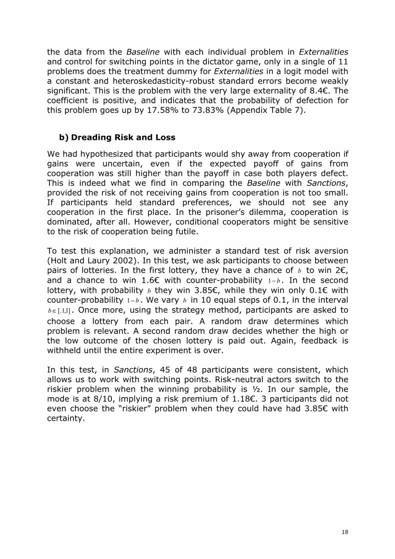
Köbberling and Wakker 2005). In this game, a participant chooses between a safe payoff of zero and a lottery. In the lottery, there is a 50% chance to gain 6€. In six equal steps of 1€, we vary the loss in the interval [2€, 7€]. Once more, we use the strategy method, all six problems are presented on one computer screen, and feedback is given only after the entire experiment is over. In the test for loss aversion, participants can make real losses. If total earnings are below 5€, the participant receives a minimum payoff of 5€. The minimum payoff is also guaranteed if overall gains from all the main and all post tests are below 5€. This is announced at the beginning of the experiment. In Sanctions, all participants were consistent in this test, which is why we work with switching points. Participants who are not loss-averse at all should accept all lotteries but the final. Effectively, in our sample most participants asked for a substantial premium for accepting the possibility of a loss, Figure 7.

05

10

15

20

25

pe

rce

nt

switc

h

1 2 3 4 5 6 7switching point

sw itching pointsLoss Aversion

Figure 7 Loss Aversion

data from 48 players in Sanctions, all of whom were consistent in this test switching points refer to the highest loss (in €) that the participant accepts the switching point is coded 1 if the participant never chooses the lottery,

and coded 7 if the participant accepts all lotteries

In none of the 11 prisoner’s dilemma problems of Sanctions does the individual switching point in the test for loss aversion have explanatory power, again using logit models with a constant and heteroskedasticity-robust standard error (Appendix Table 10). Controlling for the individual switching point does not yield a significant treatment effect in a logit regression that pools data from the Baseline with individual Sanctions problems, if the treatment effect had not already been significant in Fisher’s exact tests (Appendix Table 11). Hence loss aversion is completely uninformative for behavior in Sanctions.

21

c) Optimism

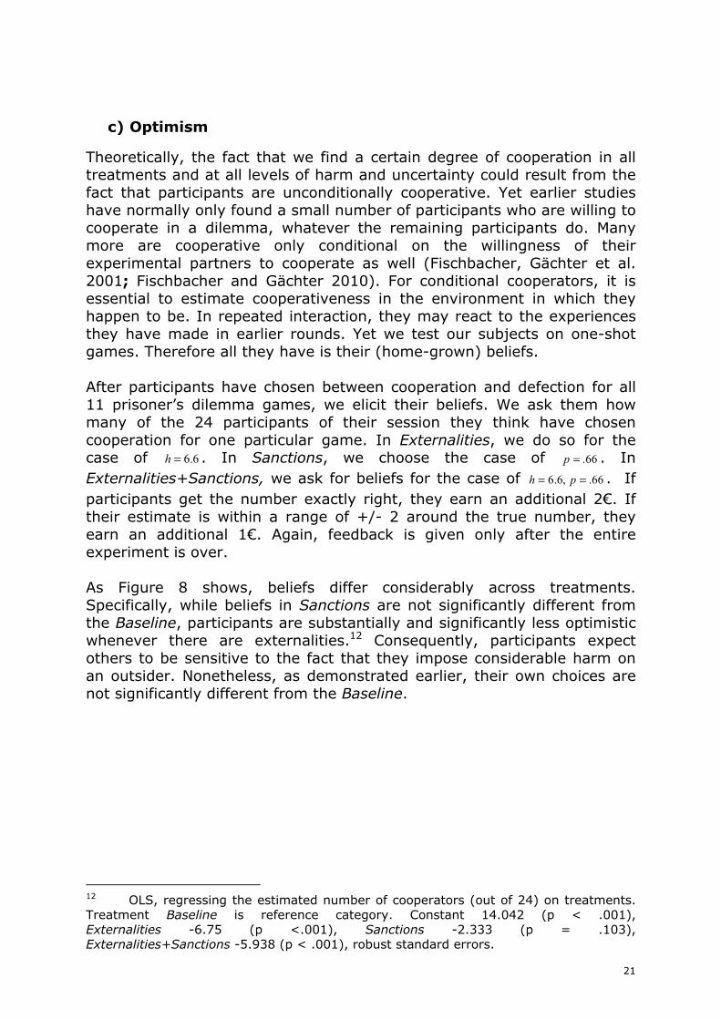
Theoretically, the fact that we find a certain degree of cooperation in all treatments and at all levels of harm and uncertainty could result from the fact that participants are unconditionally cooperative. Yet earlier studies have normally only found a small number of participants who are willing to cooperate in a dilemma, whatever the remaining participants do. Many more are cooperative only conditional on the willingness of their experimental partners to cooperate as well (Fischbacher, Gächter et al. 2001; Fischbacher and Gächter 2010). For conditional cooperators, it is essential to estimate cooperativeness in the environment in which they happen to be. In repeated interaction, they may react to the experiences they have made in earlier rounds. Yet we test our subjects on one-shot games. Therefore all they have is their (home-grown) beliefs. After participants have chosen between cooperation and defection for all 11 prisoner’s dilemma games, we elicit their beliefs. We ask them how many of the 24 participants of their session they think have chosen cooperation for one particular game. In Externalities, we do so for the case of 6.6=h . In Sanctions, we choose the case of 66.=p . In Externalities+Sanctions, we ask for beliefs for the case of 66.,6.6 == ph . If participants get the number exactly right, they earn an additional 2€. If their estimate is within a range of +/- 2 around the true number, they earn an additional 1€. Again, feedback is given only after the entire experiment is over. As Figure 8 shows, beliefs differ considerably across treatments. Specifically, while beliefs in Sanctions are not significantly different from the Baseline, participants are substantially and significantly less optimistic whenever there are externalities.12 Consequently, participants expect others to be sensitive to the fact that they impose considerable harm on an outsider. Nonetheless, as demonstrated earlier, their own choices are not significantly different from the Baseline.

12 OLS, regressing the estimated number of cooperators (out of 24) on treatments. Treatment Baseline is reference category. Constant 14.042 (p < .001), Externalities -6.75 (p <.001), Sanctions -2.333 (p = .103), Externalities+Sanctions -5.938 (p < .001), robust standard errors.

22

02

46

8F

requ

ency

0 5 10 15 20 25# cooperate

Baseline

02

46

8F

requ

ency

0 5 10 15 20 25# cooperate

harm = 6.6Externalities

02

46

8F

requ

ency

0 5 10 15 20 25# cooperate

p = .66Sanctions

02

46

8F

requ

ency

0 5 10 15 20 25# cooperate

harm = 6.6, p = .66Externalities+Sanctions

Figure 8 Beliefs

estimated number of cooperators, per treatment, in the indicated problem This already hints at the fact that participants make up for the loss in optimism by a greater individual willingness to cooperate. This is indeed what we find if we pool data from the Baseline with data from each individual Externalities problem and control for beliefs, in a logit model with a constant and heteroskedasticity-robust standard errors. We now find a significant positive treatment effect for all 11 prisoner’s dilemma problems (Appendix Table 12). This leads to the striking Result 1a: Conditional on their beliefs, however severe the harm they

impose on an outsider, active players in a simultaneous two-person prisoner’s dilemma cooperate more if cooperation is to the detriment of an outsider.

This result fits a recent finding from an experimental linear public good where contributions by active players to the public good either had a positive or a negative externality on passive bystanders. It turned out that contribution decisions were not driven by the direction of the externality, but by the comparison with bystander payoffs (Engel and Rockenbach 2011). In the present experiment, by the design of the Externality treatment, the outside player is always worse off. She can, at best, not lose, and will have her payoff reduced if at least one participant cooperates. Thereby cooperation pays a double dividend. Among the insiders, there is a chance to get gains from cooperation. If the other insider cooperates as well, both players also further distance themselves

23

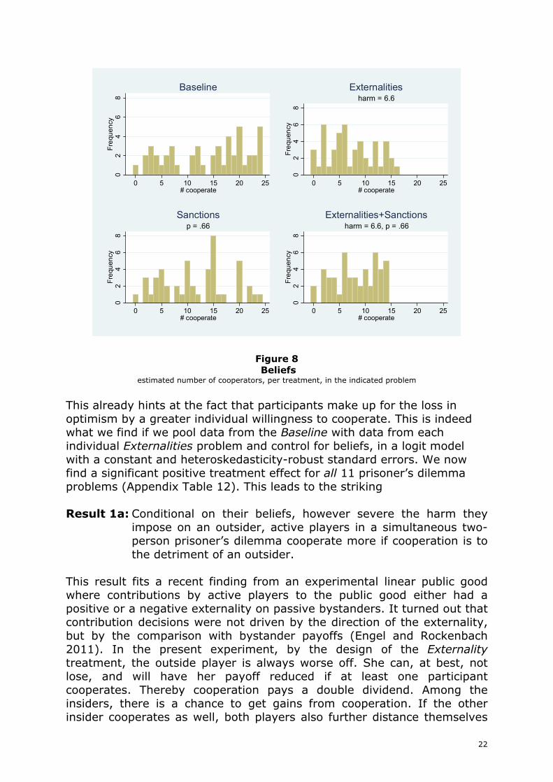
from the outsider. If not, relative payoffs depend on the size of the externality. Provided the externality is above 2.45€, even if a cooperator is exploited by the other insider she at least more strongly outperforms the outsider, compared with the only outcome she can enforce unilaterally and where both insiders earn 2.45€. Note that the benefit in terms of relative payoffs is the larger, the more pronounced the externality. By contrast, in Sanctions, if we control for beliefs, compare with the Baseline, andthe probability of getting gains from cooperation is .58, we no longer find a significant treatment effect. Yet the effect remains for a probability of .5. Hence there is still a small effect of deterrence by uncertainty (Appendix Table 13). Finally, in Externalities+Sanctions, Figure 9 shows another striking result. The left panel repeats Figure 4. If we compare treatments unconditionally, only the effect of sanctions matters. If the probability of getting gains from cooperation is low, participants cooperate significantly less; the level of harm is immaterial. Once we control for beliefs, the picture reverses, as shown in the right panel of Figure 9. Now there is significantly more cooperation when the harm imposed on the outsider is severe. By contrast, once we control for beliefs, there is no longer a significant difference from the baseline when harm is low, but the uncertainty is high (Appendix Table 14).

0.2

.4.6

.81

freq

def

ect

.3/.11.2/.18

2.1/.263.0/.34

3.9/.424.8/.5

5.7/.586.6/.66

7.5/.748.4/.82

9.3/.9

sig weakly sig insig base

Defection per Problemunconditional

0.2

.4.6

.81

freq

def

ect

.3/.11.2/.18

2.1/.263.0/.34

3.9/.424.8/.5

5.7/.586.6/.66

7.5/.748.4/.82

9.3/.9

insig sig, control for belief base

Defection per Problemconditional on beliefs

Figure 9 Externalities+Sanctions

This leads to Result 3a: When there are externalities and when, simultaneously, gains

from cooperation are uncertain, in a simultaneous two-person prisoner’s dilemma there is less cooperation with high uncertainty. Yet this effect disappears once one controls for beliefs. By contrast, if one does not control for beliefs, the fact that they inflict harm on an outsider does not significantly

24

influence participants unconditionally. Yet if one controls for beliefs, participants significantly and substantially contribute more if harm is severe.

7. Conclusions

From the perspective of basic research, our endeavor has been successful. We have one highly surprising finding: if cooperation imposes harm on an innocent outsider, this does not make cooperation less likely in a symmetric one-shot two-person prisoner’s dilemma. More interestingly even: participants believe that the externality makes it less likely that their anonymous counterparts will cooperate, but they react by a significantly higher willingness to cooperate themselves. This even holds if gains from cooperation are uncertain. We also have a second finding, which is in line with theoretical expectations: both unconditionally and conditional on the individual level of optimism, the risk of sanctions deters cooperation, even if the expected payoff of cooperation is still positive, compared with gains from mutual defection. We have designed our experiment to capture, in a stylized way, how the oligopoly dilemma is embedded in a wider social context: of the market, and of the respective legal order. It turns out that embeddedness in a market (conditionally) decreases the dilemma. Embeddedness in the legal order (mildly) increases the dilemma. From a policy perspective, our findings are less welcome news. As long as the risk of losing gains from cooperation is small, it does not induce participants to cooperate less. Since cartels are notoriously hard to detect, the detection probability will hardly ever be as high as 42%, which was necessary in our experiment to induce a change. Of course, antitrust authorities have the right to impose severe sanctions, and they increasingly do so. If behavior indeed responds to expected payoffs, harsh sanctions might suffice, even if they are rarely inflicted. Yet over-optimism (Weinstein 1980; van den Steen 2004) and the illusion of control (Langer 1975; Presson and Benassi 1996) might run counter to this effect. To which degree this matters would have to be tested in a new experiment. The behavioral effect of externalities is even more worrying. Making them salient is not only immaterial; it is even counterproductive. The latter effect, of course, requires that insiders compare themselves to outsiders. In the lab, this comparison is induced by the design of the experiment. In the field, suppliers may not (always) consider themselves to be in the same boat as their customers, which, in policy terms, would still imply that suppliers collude if ever they can. At any rate, given our findings, antitrust has no reason to expect that reticence to impose harm on those at the opposite side of the market alleviates the cartel problem. Our findings further suggest that the interaction of (small) sanctions and making the harm for the opposite market side salient does not substantially improve the situation either.

25

Of course, firms are no students. Yet for obvious methodological reasons, it is hard, if not impossible, to study the behavior of firms in the lab (Engel 2010). In most markets, there is not one outsider, but a large, often even anonymous group of buyers that suffers if sellers collude. The anonymity might make it even easier for cartelists to neglect the harm they impose on the opposite market side. On the other hand, in the field, cartelists do not only face a negative profit if the cartel is detected by the antitrust authorities. If the case is salient, it may also be covered by the press and entail reputational damage. To the extent that antitrust violations come under the purview of criminal law, managers might dread stigma on the labor market, or social disapproval, when a criminal charge is brought against them. Hiring committees might disproportionately select persons as managers with little or no social preferences. For all of these reasons we cannot give a definite answer to the question whether, in behavioral terms, oligopoly is different from a standard prisoner’s dilemma. Our results, however, suggest that two intuitive explanations for a difference are not valid: small sanctions do not induce less collusion; making harm on the opposite market side salient does not reduce collusion.

26

References

ABBINK, KLAUS (2005). Fair Salaries and the Moral Costs of Corruption. Advances in

Cognitive Economics. B. N. Kokinov. Sofia, NBU Press: ***. BECKER, GARY STANLEY (1968). "Crime and Punishment. An Economic Approach." Journal of

Political Economy 76: 169-217. BEREBY-MEYER, YOELLA and ALVIN E. ROTH (2006). "The Speed of Learning in Noisy Games.

Partial Reinforcement and the Sustainability of Cooperation." American Economic Review 96: 1029-1042.

BLANCO, MARIANA, DIRK ENGELMANN, et al. (2011). "A Within-Subject Analysis of Other-Regarding Preferences." Games and Economic Behavior ***: ***.

BOLTON, GARY E. and AXEL OCKENFELS (2000). "ERC: A Theory of Equity, Reciprocity and Competition." American Economic Review 90: 166-193.

BOLTON, GARY E. and AXEL OCKENFELS (2010). "Betrayal Aversion. Evidence from Brazil, China, Oman, Switzerland, Turkey, and the United States. Comment." American Economic Review 100: 628-633.

CHAUDHURI, ANANISH (2011). "Sustaining Cooperation in Laboratory Public Goods Experiments. A Selective Survey of the Literature." Experimental Economics 14: 47-83.

DUFWENBERG, MARTIN and GEORG KIRCHSTEIGER (2004). "A Theory of Sequential Reciprocity." Games and Economic Behavior 47: 268-298.

ELLMAN, MATTHEW and PAUL PEZANIS-CHRISTOU (2010). "Organisational Structure, Communication and Group Ethics." American Economic Review 100: ***.

ENGEL, CHRISTOPH (2007). "How Much Collusion? A Meta-Analysis on Oligopoly Experiments." Journal of Competition Law and Economics 3: 491-549.

ENGEL, CHRISTOPH (2010). "The Behaviour of Corporate Actors. A Survey of the Empirical Literature." Journal of Institutional Economics 6: 445-475.

ENGEL, CHRISTOPH and BETTINA ROCKENBACH (2011). We Are Not Alone. The Impact of Externalities on Public Good Provision.

FALK, ARMIN, ERNST FEHR, et al. (2008). "Testing Theories of Fairness - Intentions Matter." Games and Economic Behavior 62: 287-303.

FEHR, ERNST and LORENZ GOETTE (2007). ""Do Workers Work More if Wages Are High? Evidence from a Randomized Field Experiment." American Economic Review 97: 298-317.

FEHR, ERNST and KLAUS M. SCHMIDT (1999). "A Theory of Fairness, Competition, and Cooperation." Quarterly Journal of Economics 114: 817-868.

FISCHBACHER, URS (2007). "z-Tree. Zurich Toolbox for Ready-made Economic Experiments." Experimental Economics 10: 171-178.

FISCHBACHER, URS and SIMON GÄCHTER (2010). "Social Preferences, Beliefs, and the Dynamics of Free Riding in Public Good Experiments." American Economic Review 100: 541-556.

FISCHBACHER, URS, SIMON GÄCHTER, et al. (2001). "Are People Conditionally Cooperative? Evidence from a Public Goods Experiment." Economics Letters 71: 397-404.

GÄCHTER, SIMON, ERIC J. JOHNSON, et al. (2007). Individual-Level Loss Aversion in Riskless and Risky Choices.

GRECHENIG, KRISTOFFEL, ANDREAS NICKLISCH, et al. (2010). "Punishment Despite Reasonable Doubt. A Public Goods Experiment with Uncertainty over Contributions." Journal of Empirical Legal Studies 7: 847-867.

GREINER, BEN (2004). An Online Recruiting System for Economic Experiments. Forschung und wissenschaftliches Rechnen 2003. K. Kremer and V. Macho. Göttingen: 79-93.

GÜTH, WERNER and ERIC VAN DAMME (1998). "Information, Strategic Behavior, and Fairness in Ultimatum Bargaining. An Experimental Study." Journal of Mathematical Psychology 42: 227-247.

HOLT, CHARLES A. and SUSAN K. LAURY (2002). "Risk Aversion and Incentive Effects." American Economic Review 92: 1644-1655.

27

HYLTON, KEITH N. and FEI DENG (2007). "Antitrust Around the World: An Empirical Analysis of the Scope of Competition Laws and Their Effects’(2007)." Antitrust Law Journal 74: 271-341.

KAHN, LAWRENCE M. and J. KEITH MURNIGHAN (1993). "Conjecture, Uncertainty, and Cooperation in Prisoner's Dilemma Games. Some Experimental Evidence." Journal of Economic Behavior & Organization 22: 91-117.

KÖBBERLING, VERONIKA and PETER P. WAKKER (2005). "An Index of Loss Aversion." Journal of Economic Theory 122: 119-131.

KUNREUTHER, HOWARD, GABRIEL SILVASI, et al. (2009). "Bayesian Analysis of Deterministic and Stochastic Prisoner’s Dilemma Games." Judgement and Decision Making 4: 363-384.

LANGER, ELLEN J. (1975). "The Illusion of Control." Journal of Personality and Social Psychology 32: 311-328.

LEDYARD, JOHN O. (1995). Public Goods. A Survey of Experimental Research. The Handbook of Experimental Economics. J. H. Kagel and A. E. Roth. Princeton, NJ, Princeton University Press: 111-194.

PRESSON, PAUL K. and VICTOR A. BENASSI (1996). "Illusion of Control. A Meta-Analytic Review." Journal of Social Behavior and Personality 11: 493-510.

RABIN, MATTHEW (1993). "Incorporating Fairness into Game Theory and Economics." American Economic Review 83: 1281-1302.

RABIN, MATTHEW (2000). "Risk Aversion and Expected-Utility Theory. A Calibration Theorem." Econometrica 68: 1281-1293.

RABIN, MATTHEW and RICHARD THALER (2001). "Anomalies - Risk Aversion." Journal of Economic Perspectives 15: 219-232.

RAPOPORT, ANATOL and ALBERT M. CHAMMAH (1965). Prisoner's Dilemma. A Study in Conflict and Cooperation. Ann Arbor,, University of Michigan Press.

SABATER-GRANDE, GERARDO and NIKOLAOS GEORGANTZIS (2002). "Accounting for Risk Aversion in Repeated Prisoners’ Dilemma Games. An Experimental Test." Journal of Economic Behavior & Organization 48: 37-50.

SELTEN, REINHARD (1967). Die Strategiemethode zur Erforschung des eingeschränkt rationalen Verhaltens im Rahmen eines Oligopolexperiments. Beiträge zur experimentellen Wirtschaftsforschung. E. Sauermann. Tübingen, Mohr: 136-168.

TIROLE, JEAN (1988). The Theory of Industrial Organization. Cambridge, Mass., MIT Press. TVERSKY, AMOS and DANIEL KAHNEMAN (1992). "Advances in Prospect Theory. Cumulative

Representation of Uncertainty." Journal of Risk and Uncertainty 5: 297-323. VAN DEN STEEN, ERIC (2004). "Rational Overoptimism (and Other Biases)." American

Economic Review 94: 1141-1151. WEINSTEIN, NEIL D. (1980). "Unrealistic Optimism about Future Life Events." Journal of

Personality and Social Psychology 39(5): 806-820. ZELMER, JENNIFER (2003). "Linear Public Goods. A Meta-Analysis." Experimental Economics

6: 299-310.

28

Appendix

I. Instructions The Instructions for the four treatments differ only in Part 1. The rest is identical. Therefore we report first the full instructions of the baseline treatment and afterwards only part 1 of the other treatments.

a. Baseline

Welcome to our experiment. Please remain quiet and do not talk to the other participants during the experiment. If you have any questions, please give us a signal. We will answer your queries individually.

Course of Events

The experiment is divided into four parts. We will distribute separate instructions for each of the four parts of the experiment. Please read these instructions carefully and make your decisions only after taking an appropriate amount of time to reflect on the situations, and after we have fully answered any questions you may have. Only when all participants have decided will we move on to the next part of the experiment. All of your decisions will be treated anonymously.

Your Payoff

At the end of the experiment, we will give you your payoff in cash. Each of you will receive the earnings resulting from the decisions you will have made in the course of the experiment. It is possible to make a loss in one part of the experiment. These losses will be subtracted from the earnings in the other parts.

Thus:

Total payment =

+ Earnings from Part 1 + Earnings from Part 2 + Earnings from Part 3 + Earnings from Part 4 (min. 5€)

In Part 2, however, losses are possible, too. Should you incur losses, these will be deducted from your earnings from Part 1, Part 3, or Part 4. (The possibility of losses in Part 2 is limited, however; you will definitely receive a total payment that is on the plus side of the balance.) If you earn on the whole less than 5€, you will get a minimum payment of 5€.

29

We will explain the details of how your payoff is made up for each of the four parts separately. In each of the four parts, possible payoffs are given in Euro, which is the currency you will be paid in.

Part 1

The basic idea of this part of the experiment is as follows: you are anonymously paired by us with another participant. You and the other participant will make a total of eleven decisions.

Only one pair of decisions will determine your payoff. This procedure is explained below.

We will show you eleven tables that look as follows:

Type B Above Below Above 5€, 5€ 0€, 10€

Type A Below 10€, 0€ z€, z€

We will let you know at the start whether you are a Type A or a Type B participant. (You will probably notice that the payments given to both types are symmetrical; the distinction between Type A and Type B is solely for the purpose of explaining the experiment.)

The decisions Above or Below determine the payoffs to you and the other participant. In each of the four cells of the table, the figure on the left denotes A’s profit, while the figure on the right denotes B’s profit.

For instance, if Type A chooses the option Above and Type B chooses the option Above, then both receive a payment of 5€. If Type A chooses Above and Type B chooses Below, then Type A receives zero profit and Type B gets 10€. The same is valid for a Below/Above constellation. Finally, if Type A chooses Below and Type B chooses Below, then both receive a payment of z€.

What does the z stand for? z is varied in the following eleven tables; all other payments remain unchanged. You have to decide on all eleven tables (Above or Below). Please mark your decision by clicking on the appropriate box shown on your screen.

You will be free to address each of the eleven tables separately, making your decisions independently of the other tables. You can also make the same decision all the time. This is entirely up to you.

Please note, once again, that only one of the eleven decision pairs will be relevant for your payoff. We will choose one of the eleven tables at

30

random at the end. Your decision for the table that is drawn by lot and the other participant’s decision for the same table determine the payoff in this part of the experiment.

Let us first begin with some test questions. (The aim of these questions is merely to verify whether all participants have fully understood the instructions. Neither the questions nor the answers have anything to do with your final payment.) Then the screen on which your actual decisions are marked will appear.

Do you have any further questions?

Part 1a

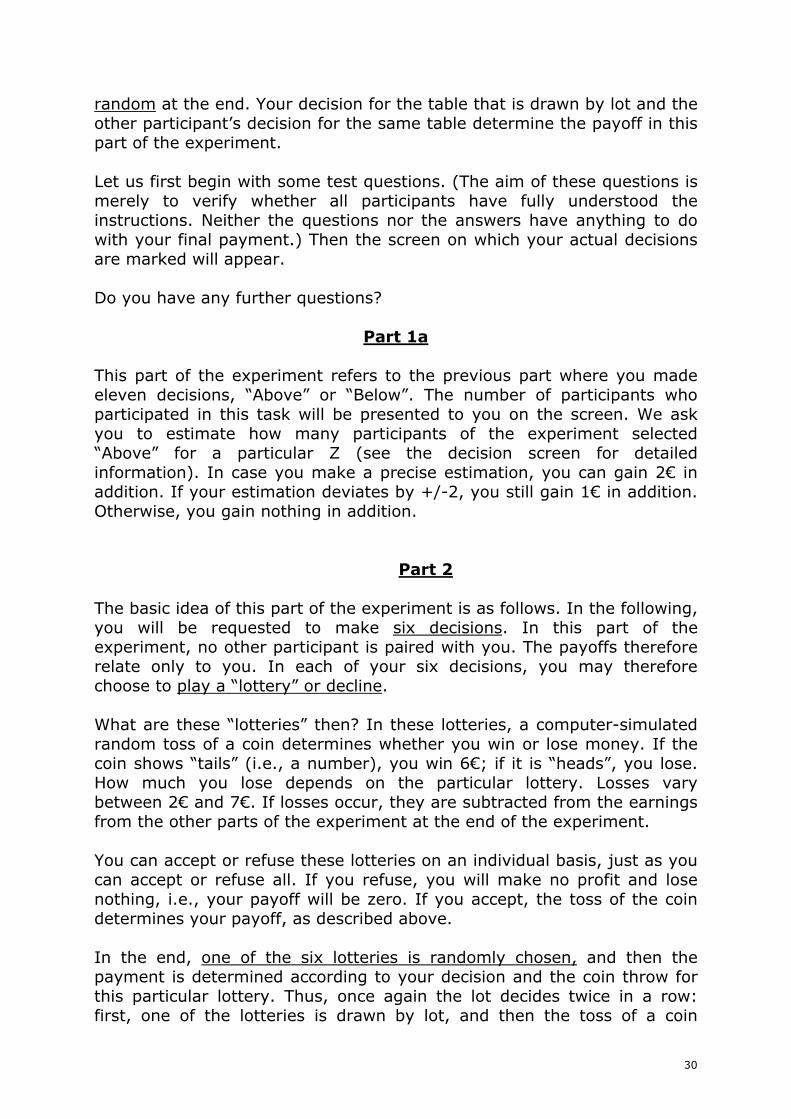
This part of the experiment refers to the previous part where you made eleven decisions, “Above” or “Below”. The number of participants who participated in this task will be presented to you on the screen. We ask you to estimate how many participants of the experiment selected “Above” for a particular Z (see the decision screen for detailed information). In case you make a precise estimation, you can gain 2€ in addition. If your estimation deviates by +/-2, you still gain 1€ in addition. Otherwise, you gain nothing in addition.

Part 2

The basic idea of this part of the experiment is as follows. In the following, you will be requested to make six decisions. In this part of the experiment, no other participant is paired with you. The payoffs therefore relate only to you. In each of your six decisions, you may therefore choose to play a “lottery” or decline.

What are these “lotteries” then? In these lotteries, a computer-simulated random toss of a coin determines whether you win or lose money. If the coin shows “tails” (i.e., a number), you win 6€; if it is “heads”, you lose. How much you lose depends on the particular lottery. Losses vary between 2€ and 7€. If losses occur, they are subtracted from the earnings from the other parts of the experiment at the end of the experiment.

You can accept or refuse these lotteries on an individual basis, just as you can accept or refuse all. If you refuse, you will make no profit and lose nothing, i.e., your payoff will be zero. If you accept, the toss of the coin determines your payoff, as described above.

In the end, one of the six lotteries is randomly chosen, and then the payment is determined according to your decision and the coin throw for this particular lottery. Thus, once again the lot decides twice in a row: first, one of the lotteries is drawn by lot, and then the toss of a coin

31

decides whether or not you win in this lottery – on condition that you have decided to go for the lottery.

Let us first begin with some test questions. (The aim of these questions is merely to verify whether all participants have fully understood the instructions. Neither the questions nor the answers have anything to do with your final payment.) Then the screen on which your actual decisions are marked will appear.

Part 3

This part of the experiment is as follows: one Type X participant has to decide between two situations (1 or 2). His decision influences his own payoff, and the payoff of one other randomly paired Type Y participant, as follows:

Situation 1: Type X receives a payoff, determined by lot, of 5€ or 10€, Type Y receives a payoff of zero Euro. The likelihood with which Type X either receives 5€ or 10€ is systematically varied in the following table. Type X must make a decision for each of the eleven constellations (a total of 11 decisions).

Situation 2 remains the same for all 11 constellations: Type X and Type Y both receive 5€.

In this part, all participants must initially make their decisions in the role of Type X.

We will proceed with the payoff as follows:

− The lot is drawn to determine whether your payments, following

your own decisions, classify you as a Type X or a (passive) Type Y. We will draw one half of the group as Type X and the other as Type Y.

− The next draw pairs each Type Y participant with a Type X participant.

− Finally, the third draw determines one single payoff-relevant situation out of the total of eleven situations. Therefore, one out of the eleven decisions emerges as the basis for payoff. With a probability of ½, it will be your own decision, and with the same likelihood it will be another participant’s decision.

32

Example for Part 3

Profit With likelihood of

You 10€ 30% 5€ 70%

Other participant 0€ 100% 1

Your decision 2

Both 5€ 100%

As stated above, all participants will make eleven decisions of this kind. Please mark your decision by clicking on the appropriate box.

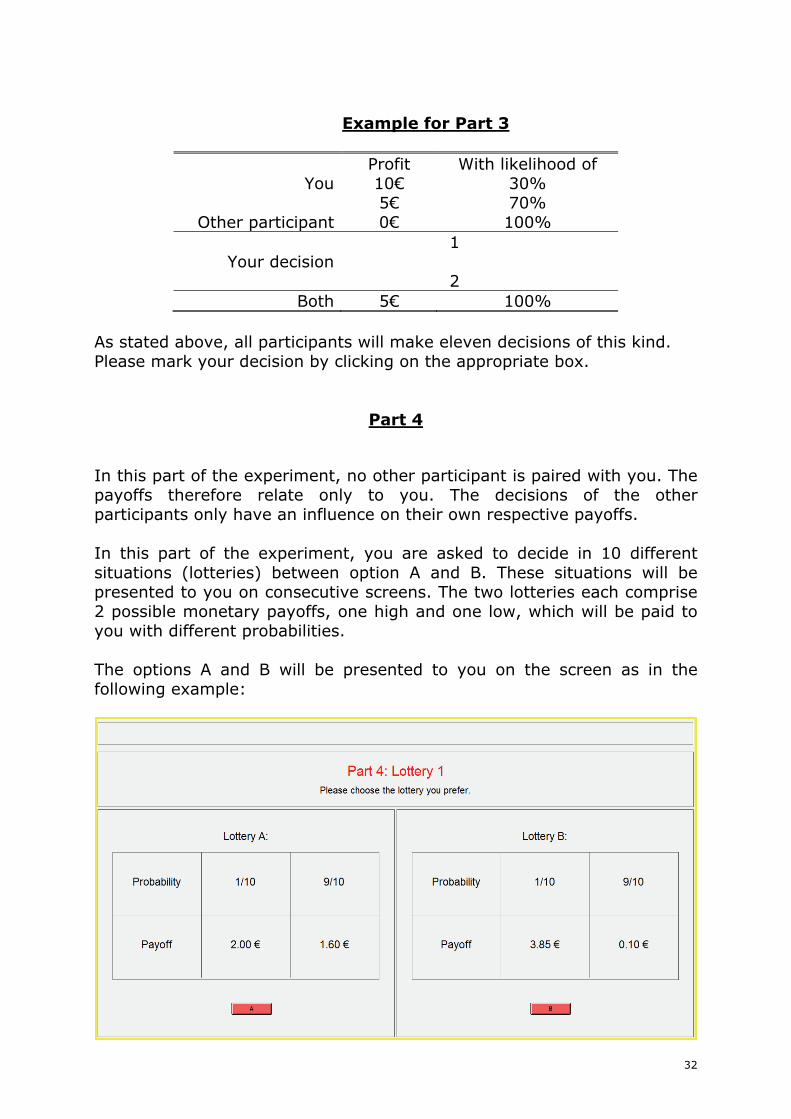
Part 4 In this part of the experiment, no other participant is paired with you. The payoffs therefore relate only to you. The decisions of the other participants only have an influence on their own respective payoffs. In this part of the experiment, you are asked to decide in 10 different situations (lotteries) between option A and B. These situations will be presented to you on consecutive screens. The two lotteries each comprise 2 possible monetary payoffs, one high and one low, which will be paid to you with different probabilities. The options A and B will be presented to you on the screen as in the following example:

33

The computer uses a random draw program, which assigns you payments exactly according to the denoted probabilities. For the above example, this means: Option A obtains a payoff of 2 Euro with a probability of 10% and a payoff of 1.60 Euro with a probability of 90%. Option B obtains a payoff of 3.85 Euro with a probability of 10% and a payoff of 0.10 Euro with a probability of 90%. Now you have to click on the particular option you decide for. Please note that at the end of the experiment only one of the 10 situations will eventually be paid. Yet, each of the situations can be randomly chosen with equal probability to be the payoff-relevant one. After this, a draw will determine whether for the payoff-relevant situation the high payoff (2.00 Euro or 3.85 Euro) or the low payoff (1.60 Euro or 0.10 Euro) will be paid.

b. Externalities

Part 1

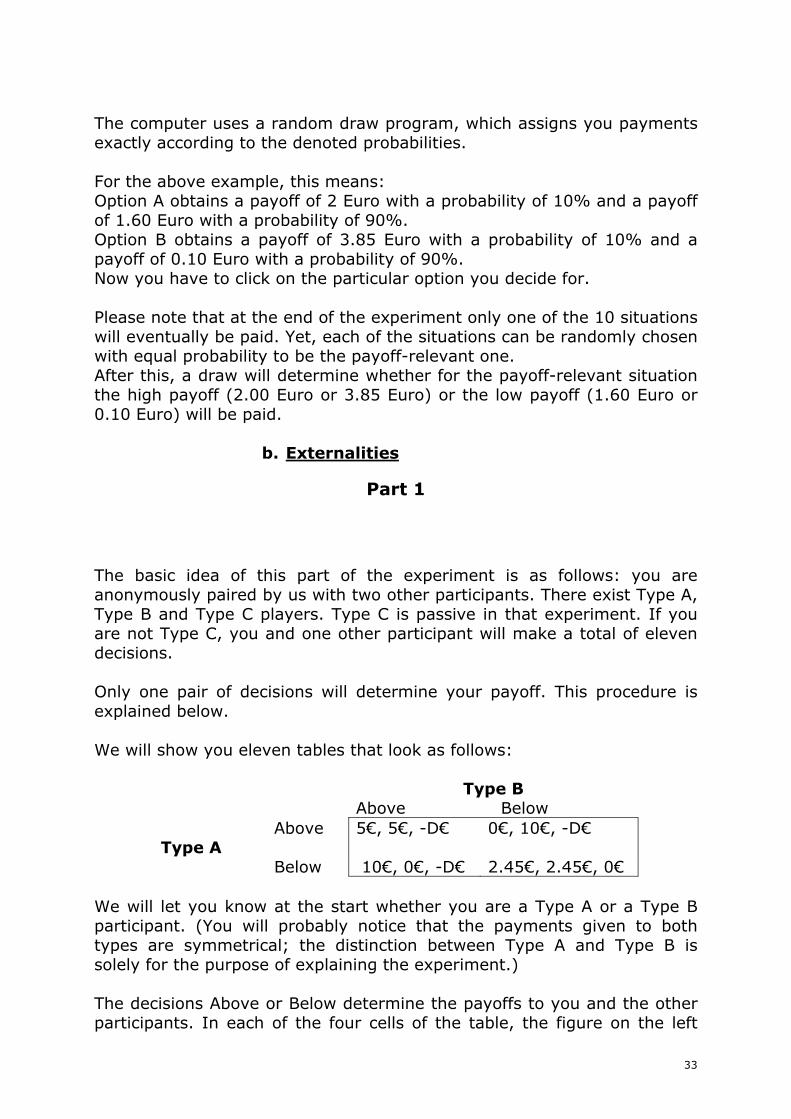
The basic idea of this part of the experiment is as follows: you are anonymously paired by us with two other participants. There exist Type A, Type B and Type C players. Type C is passive in that experiment. If you are not Type C, you and one other participant will make a total of eleven decisions. Only one pair of decisions will determine your payoff. This procedure is explained below. We will show you eleven tables that look as follows:

Type B Above Below Above 5€, 5€, -D€ 0€, 10€, -D€ Type A Below 10€, 0€, -D€ 2.45€, 2.45€, 0€

We will let you know at the start whether you are a Type A or a Type B participant. (You will probably notice that the payments given to both types are symmetrical; the distinction between Type A and Type B is solely for the purpose of explaining the experiment.) The decisions Above or Below determine the payoffs to you and the other participants. In each of the four cells of the table, the figure on the left

34

denotes A’s profit, while the figure on the right denotes B’s profit. Type C receives either –D€ or 0€, depending on the decisions of Type A and B. For instance, if Type A chooses the option Above and Type B chooses the option Above, then both receive a payment of 5€ and Type C receives –D€. If Type A chooses Above and Type B chooses Below, then Type A receives zero profit, Type B gets 10€, and Type C receives –D€. The same is valid for a Below/Above constellation. Finally, if Type A chooses Below and Type B chooses Below, then both receive a payment of 2.45€ and Type C receives 0€. What does the D stand for? D is varied in the following eleven tables. It is an absolute value that will be paid in €; all other payments remain unchanged. You have to decide on all eleven tables (Above or Below). Please mark your decision by clicking on the appropriate box shown on your screen. You will be free to address each of the eleven tables separately, making your decisions independently of the other tables. You can also make the same decision all the time. This is entirely up to you. Please note, once again, that only one of the eleven decision pairs will be relevant for your payoff. We will choose one of the eleven tables at random at the end. Your decision for the table that is drawn by lot and the other participant’s decision for the same table determine the payoff in this part of the experiment. Let us first begin with some test questions. (The aim of these questions is merely to verify whether all participants have fully understood the instructions. Neither the questions nor the answers have anything to do with your final payment.) Then the screen on which your actual decisions are marked will appear. Do you have any further questions?

c. Sanctions

Part 1

The basic idea of this part of the experiment is as follows: you are anonymously paired by us with another participant. You and the other participant will make a total of eleven decisions.

Only one pair of decisions will determine your payoff. This procedure is explained below.

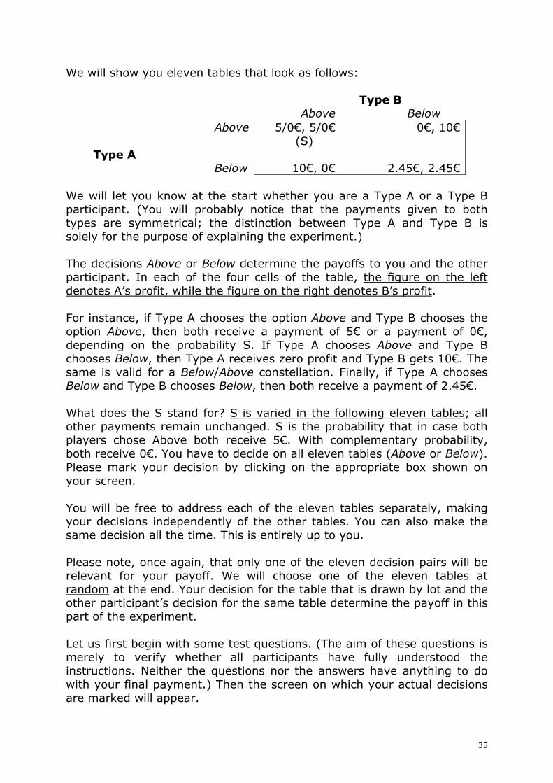
35

We will show you eleven tables that look as follows:

Type B Above Below Above 5/0€, 5/0€

(S) 0€, 10€

Type A Below 10€, 0€ 2.45€, 2.45€

We will let you know at the start whether you are a Type A or a Type B participant. (You will probably notice that the payments given to both types are symmetrical; the distinction between Type A and Type B is solely for the purpose of explaining the experiment.)

The decisions Above or Below determine the payoffs to you and the other participant. In each of the four cells of the table, the figure on the left denotes A’s profit, while the figure on the right denotes B’s profit.

For instance, if Type A chooses the option Above and Type B chooses the option Above, then both receive a payment of 5€ or a payment of 0€, depending on the probability S. If Type A chooses Above and Type B chooses Below, then Type A receives zero profit and Type B gets 10€. The same is valid for a Below/Above constellation. Finally, if Type A chooses Below and Type B chooses Below, then both receive a payment of 2.45€.

What does the S stand for? S is varied in the following eleven tables; all other payments remain unchanged. S is the probability that in case both players chose Above both receive 5€. With complementary probability, both receive 0€. You have to decide on all eleven tables (Above or Below). Please mark your decision by clicking on the appropriate box shown on your screen.

You will be free to address each of the eleven tables separately, making your decisions independently of the other tables. You can also make the same decision all the time. This is entirely up to you.

Please note, once again, that only one of the eleven decision pairs will be relevant for your payoff. We will choose one of the eleven tables at random at the end. Your decision for the table that is drawn by lot and the other participant’s decision for the same table determine the payoff in this part of the experiment.

Let us first begin with some test questions. (The aim of these questions is merely to verify whether all participants have fully understood the instructions. Neither the questions nor the answers have anything to do with your final payment.) Then the screen on which your actual decisions are marked will appear.

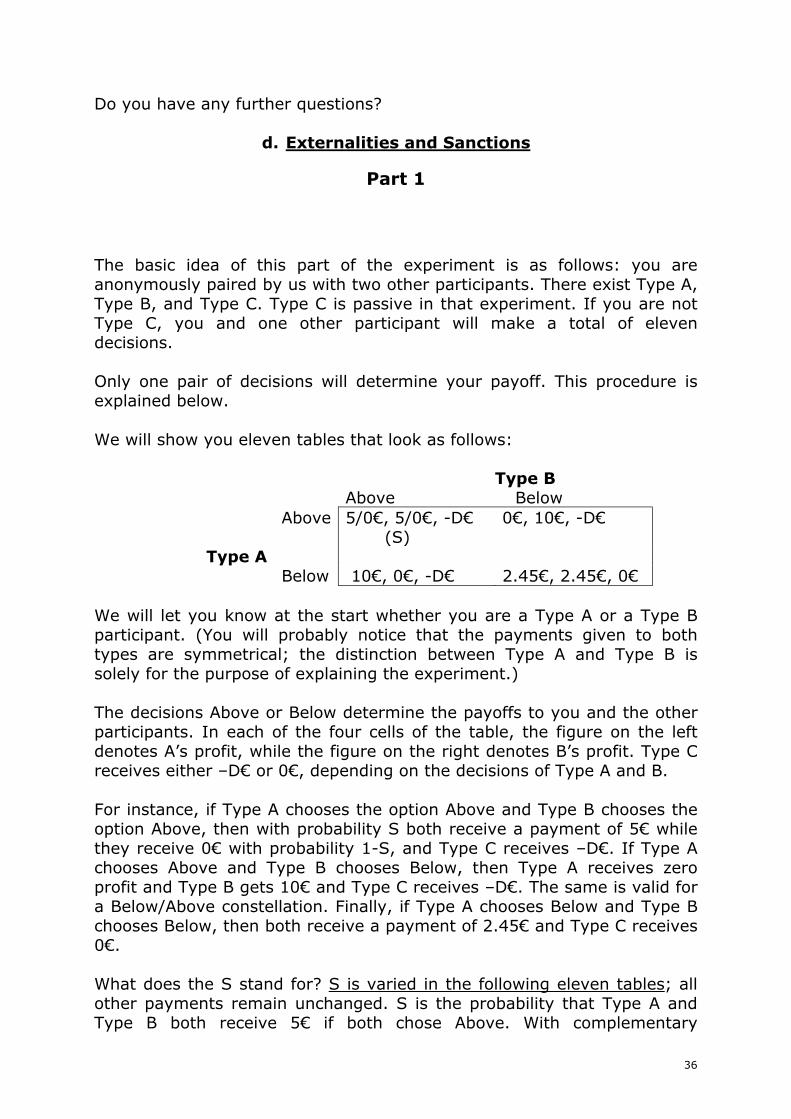
36

Do you have any further questions?

d. Externalities and Sanctions

Part 1

The basic idea of this part of the experiment is as follows: you are anonymously paired by us with two other participants. There exist Type A, Type B, and Type C. Type C is passive in that experiment. If you are not Type C, you and one other participant will make a total of eleven decisions. Only one pair of decisions will determine your payoff. This procedure is explained below. We will show you eleven tables that look as follows:

Type B Above Below Above 5/0€, 5/0€, -D€

(S) 0€, 10€, -D€

Type A Below 10€, 0€, -D€ 2.45€, 2.45€, 0€

We will let you know at the start whether you are a Type A or a Type B participant. (You will probably notice that the payments given to both types are symmetrical; the distinction between Type A and Type B is solely for the purpose of explaining the experiment.) The decisions Above or Below determine the payoffs to you and the other participants. In each of the four cells of the table, the figure on the left denotes A’s profit, while the figure on the right denotes B’s profit. Type C receives either –D€ or 0€, depending on the decisions of Type A and B. For instance, if Type A chooses the option Above and Type B chooses the option Above, then with probability S both receive a payment of 5€ while they receive 0€ with probability 1-S, and Type C receives –D€. If Type A chooses Above and Type B chooses Below, then Type A receives zero profit and Type B gets 10€ and Type C receives –D€. The same is valid for a Below/Above constellation. Finally, if Type A chooses Below and Type B chooses Below, then both receive a payment of 2.45€ and Type C receives 0€. What does the S stand for? S is varied in the following eleven tables; all other payments remain unchanged. S is the probability that Type A and Type B both receive 5€ if both chose Above. With complementary

37

probability, both receive 0. What does the D stand for? D is varied in the following eleven tables. It is an absolute value that will be paid in €. All payments, except those depending on D and S, remain unchanged in all eleven situations. You have to decide on all eleven tables (Above or Below). Please mark your decision by clicking on the appropriate box shown on your screen. You will be free to address each of the eleven tables separately, making your decisions independently of the other tables. You can also make the same decision all the time. This is entirely up to you. Please note, once again, that only one of the eleven decision pairs will be relevant for your payoff. We will choose one of the eleven tables at random at the end. Your decision for the table that is drawn by lot and the other participant’s decision for the same table determine the payoff in this part of the experiment. Let us first begin with some test questions. (The aim of these questions is merely to verify whether all participants have fully understood the instructions. Neither the questions nor the answers have anything to do with your final payment.) Then the screen on which your actual decisions are marked will appear. Do you have any further questions?

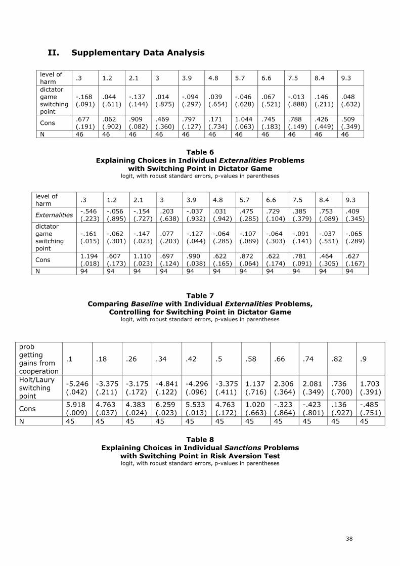
38

II. Supplementary Data Analysis

level of harm .3 1.2 2.1 3 3.9 4.8 5.7 6.6 7.5 8.4 9.3

dictator game switching point

-.168 (.091)

.044 (.611)

-.137 (.144)

.014 (.875)

-.094 (.297)

.039 (.654)

-.046 (.628)

.067 (.521)

-.013 (.888)

.146 (.211)

.048 (.632)

Cons .677 (.191)

.062 (.902)

.909 (.082)

.469 (.360)

.797 (.127)

.171 (.734)

1.044 (.063)

.745 (.183)

.788 (.149)

.426 (.449)

.509 (.349)

N 46 46 46 46 46 46 46 46 46 46 46

Table 6 Explaining Choices in Individual Externalities Problems

with Switching Point in Dictator Game logit, with robust standard errors, p-values in parentheses

level of harm .3 1.2 2.1 3 3.9 4.8 5.7 6.6 7.5 8.4 9.3

Externalities -.546 (.223)

-.056 (.895)

-.154 (.727)

.203 (.638)

-.037 (.932)

.031 (.942)

.475 (.285)

.729 (.104)

.385 (.379)

.753 (.089)

.409 (.345)

dictator game switching point

-.161 (.015)

-.062 (.301)

-.147 (.023)

.077 (.203)

-.127 (.044)

-.064 (.285)

-.107 (.089)

-.064 (.303)

-.091 (.141)

-.037 (.551)

-.065 (.289)

Cons 1.194 (.018)

.607 (.173)

1.110 (.023)

.697 (.124)

.990 (.038)

.622 (.165)

.872 (.064)

.622 (.174)

.781 (.091)

.464 (.305)

.627 (.167)

N 94 94 94 94 94 94 94 94 94 94 94

Table 7

Comparing Baseline with Individual Externalities Problems, Controlling for Switching Point in Dictator Game

logit, with robust standard errors, p-values in parentheses

prob getting gains from cooperation

.1 .18 .26 .34 .42 .5 .58 .66 .74 .82 .9

Holt/Laury switching point

-5.246 (.042)

-3.375(.211)

-3.175 (.172)

-4.841(.122)

-4.296(.096)

-3.375(.411)

1.137 (.716)

2.306 (.364)

2.081 (.349)

.736 (.700)

1.703 (.391)

Cons 5.918 (.009)

4.763 (.037)

4.383 (.024)

6.259 (.023)

5.533 (.013)

4.763 (.172)

1.020 (.663)

-.323 (.864)

-.423 (.801)

.136 (.927)

-.485 (.751)

N 45 45 45 45 45 45 45 45 45 45 45

Table 8 Explaining Choices in Individual Sanctions Problems

with Switching Point in Risk Aversion Test logit, with robust standard errors, p-values in parentheses

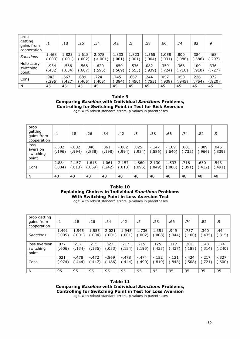
39

prob getting gains from cooperation

.1 .18 .26 .34 .42 .5 .58 .66 .74 .82 .9

Sanctions 1.468 (.003)

1.823 (.001)

1.618 (.002)

2.078 (<.001)

1.833 (.001)

1.823 (.001)

1.565 (.004)

1.058 (.031)

.800 (.088)

.384 (.386)

.468 (.297)

Holt/Laury switching point

-.934 (.432)

-.536 (.634)

-.568 (.607)

-.620 (.595)

-.650 (.569)

-.536 (.653)

.082 (.939)

.359 (.724)

.368 (.710)

.109 (.910)

.336 (.727)

Cons .942 (.295)

.667 (.427)

.689 (.405)

.724 (.405)

.745 (.384)

.667 (.450)

.244 (.755)

.057 (.939)

.050 (.945)

.226 (.754)

.072 (.920)

N 45 45 45 45 45 45 45 45 45 45 45

Table 9 Comparing Baseline with Individual Sanctions Problems, Controlling for Switching Point in Test for Risk Aversion

logit, with robust standard errors, p-values in parentheses

prob getting gains from cooperation

.1 .18 .26 .34 .42 .5 .58 .66 .74 .82 .9

loss aversion switching point

-.302 (.196)

-.002 (.994)

.046 (.838)

.361 (.198)

-.002 (.994)

.025 (.934)

-.147 (.586)

-.109 (.640)

.081 (.732)

-.009 (.966)

.045 (.839)

Cons 2.884 (.004)

2.157 (.013)

1.613 (.059)

1.061 (.242)

2.157 (.013)

1.860 (.095)

2.130 (.049)

1.593 (.080)

.718 (.391)

.630 (.412)

.543 (.491)

N 48 48 48 48 48 48 48 48 48 48 48

Table 10 Explaining Choices in Individual Sanctions Problems

With Switching Point in Loss Aversion Test logit, with robust standard errors, p-values in parentheses

prob getting gains from cooperation

.1 .18 .26 .34 .42 .5 .58 .66 .74 .82 .9

Sanctions 1.491 (.005)

1.945 (.001)

1.555 (.004)

2.021 (.001)

1.945 (.001)

1.736 (.002)

1.351 (.008)

.949 (.044)

.757 (.100)

.340 (.435)

.444 (.315)

loss aversion switching point

.077 (.606)

.217 (.134)

.215 (.136)

.327 (.033)

.217 (.134)

.215 (.195)

.125 (.433)

.117 (.437)

.201 (.188)

.143 (.314)

.174 (.240)

Cons .021 (.974)

-.478 (.444)

-.472 (.447)

-.869 (.186)

-.478 (.444)

-.474 (.490)

-.152 (.819)

-.121 (.848)

-.424 (.508)

-.217 (.721)

-.327 (.600)

N 95 95 95 95 95 95 95 95 95 95 95

Table 11 Comparing Baseline with Individual Sanctions Problems, Controlling for Switching Point in Test for Loss Aversion

logit, with robust standard errors, p-values in parentheses

40

level of harm .3 1.2 2.1 3 3.9 4.8 5.7 6.6 7.5 8.4 9.3

ext -2.205 (0.001)

-2.025 (0.002)

-1.738 (0.004)

-1.965 (0.004)

-2.056 (0.004)

-2.091 (0.002)

-1.641 (0.016)

-1.418 (0.026)

-1.747 (0.01)

-1.602 (0.02)

-1.947 (0.008)

belief -0.233 (<.001)

-0.248 (<.001)

-0.228 (<.001)

-0.28 (<.001)

-0.277 (<.001)

-0.268 (<.001)

-0.302 (<.001)

-0.291 (<.001)

-0.299 (<.001)

-0.315 (<.001)

-0.324 (<.001)

cons 3.779 (<.001)

4.028 (<.001)

3.696 (<.001)

4.555 (<.001)

4.502 (<.001)

4.354 (<.001)

4.927 (<.001)

4.736 (<.001)

4.869 (<.001)

5.147 (<.001)

5.288 (<.001)

Table 12

Comparing Baseline with Individual Externalities Problems, Controlling for Beliefs

logit, with robust standard errors, p-values in parentheses

prob getting gains from cooperation

.1 .18 .26 .34 .42 .5 .58 .66 .74 .82 .9

sanc 1.371 (0.019)

1.831(0.006)

1.379 (0.019)

1.931(0.007)

1.863(0.008)

1.628(0.014)

1.209(0.055)

0.638(0.265)

0.362 (0.495)

-0.111(0.824)

-0.034(0.948)

belief -0.178 (<.001)

-0.205 (<.001)

-0.204 (<.001)

-0.285(<.001)

-0.235(<.001)

-0.25(<.001)

-0.299(<.001)

-0.274(<.001)

-0.236 (<.001)

-0.204(<.001)

-0.225(<.001)

cons 2.905 (<.001)

3.329(<.001)

3.31 (<.001)

4.644(<.001)

3.815(<.001)

4.068(<.001)

4.877(<.001)

4.466(<.001)

3.835 (<.001)

3.318(<.001)

3.66(<.001)

Table 13

Comparing Baseline with Individual Sanctions Problems, Controlling for Beliefs

logit, with robust standard errors, p-values in parentheses

param combi .3/.1 1.2/.18 2.1/.26 3.0/.34 3.9/.42 4.8/.5 5.7/.58 6.6/.66 7.5/.74 8.4/.82 9.3/.9

both 0.137 0.782

0.228 0.659

-0.016 0.975

0.019 0.976

0.019 0.976

-1.077 0.093

-1.391 0.031

-1.945 0.009

-1.999 0.004

-1.999 0.001

-2.212 0.001

belief -0.211 (<.001)

-0.225 (<.001)

-0.237 (<.001)

-0.297 (<.001)

-0.297 (<.001)

-0.313 (<.001)

-0.32 (<.001)

-0.382 (<.001)

-0.351 (<.001)

-0.288 (<.001)

-0.287 (<.001)

cons 3.426 (<.001)

3.653 (<.001)

3.851 (<.001)

4.835 (<.001)

4.835 (<.001)

5.107 (<.001)

5.224 (<.001)

6.273 (<.001)

5.76 (<.001)

4.689 (<.001)

4.67 (<.001)

Table 14

Comparing Baseline with Individual Externalities+Sanctions Problems, Controlling for Beliefs

logit, with robust standard errors, p-values in parentheses