October,25 2005 Scripps Institution of Oceanography

An Alternative Method to Building Adjoints

Julia LevinRutgers University

Andrew Bennett “Inverse Modeling of the Ocean and Atmosphere”

Carl Wunsch “Ocean Circulation Inverse Problem”

Julia Muccino’s Inverse Ocean Modeling Website http://216.216.95.110/index.cfm?fuseaction=home.main

Different ways of building adjoints

“Symbolic” “Analytic” Automatic

Outline

• Background: basic ideas of building adjoint operators on a simple 1D advection equation.

• Continuous and discrete adjoint operators

• Comparison between “analytic” and “symbolic” approaches to building discrete adjoint operators.

• Examples

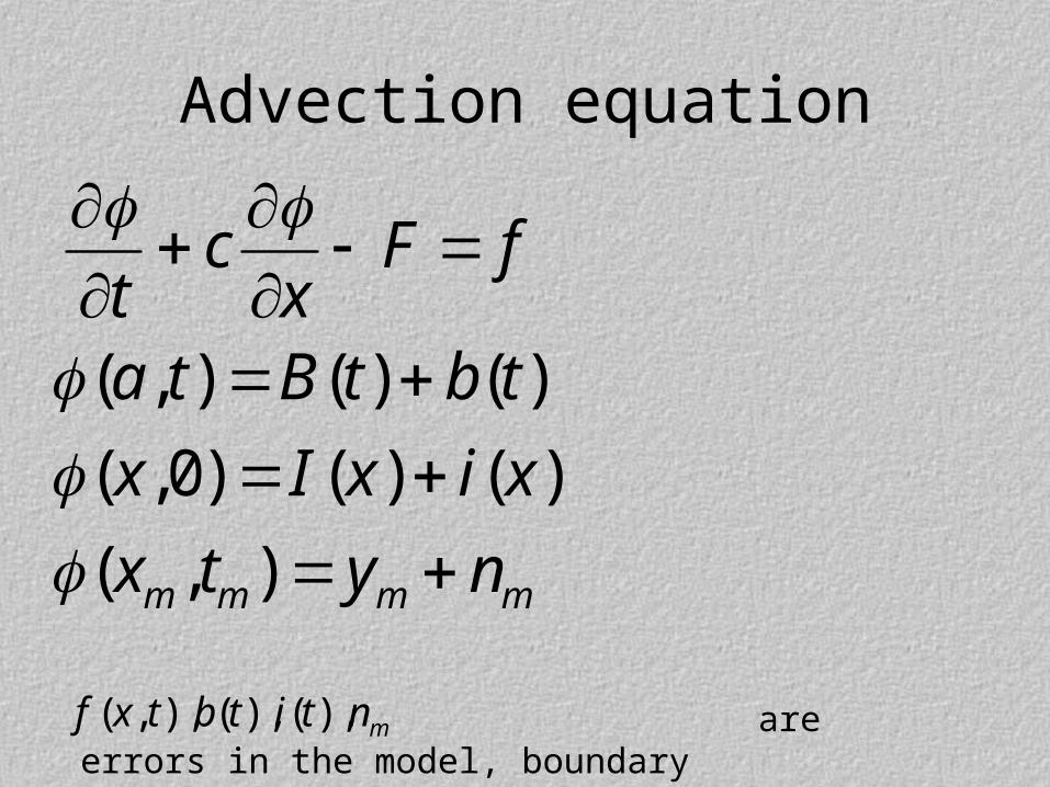
Advection equation

( , ) ( ) ( )

( ,0) ( ) ( )

( , )m m m m

c F ft xa t B t b t

x I x i x

x t y n

are errors in the model, boundary conditions, initial conditions and data respectively

mntitbtxf ),(),(),,(

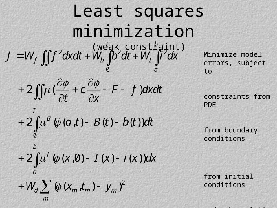
Least squares minimization (weak constraint)

2 2 2

0

0

2

2 ( )

2 ( ( , ) ( ) ( ))

2 ( ( ,0) ( ) ( ))

( ( , ) )

T b

f b I

a

TB

bI

a

d m m mm

J W f dxdt W b dt W i dx

c F f dxdtt x

a t B t b t dt

x I x i x dx

W x t y

Minimize model errors, subject to

constraints from PDE

from boundary conditions

from initial conditions

and make solution closest to the data

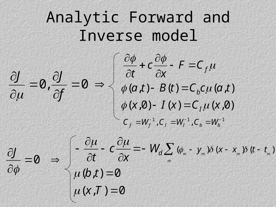
Analytic Forward and Inverse model

( , ) ( ) ( , )

( ,0) ( ) ( ,0)

f

b

I

c F Ct xa t B t C c a t

x I x C x

( ) ( ) ( )

( , ) 0

( , ) 0

m m m m

m

d y x x t tc Wt xb t

x T

0,0f

JJ

0J

111 ,, bbIIff WCWCWC

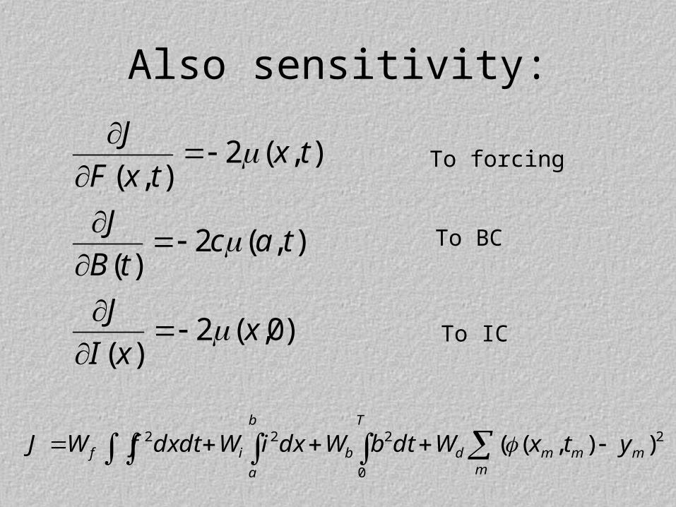
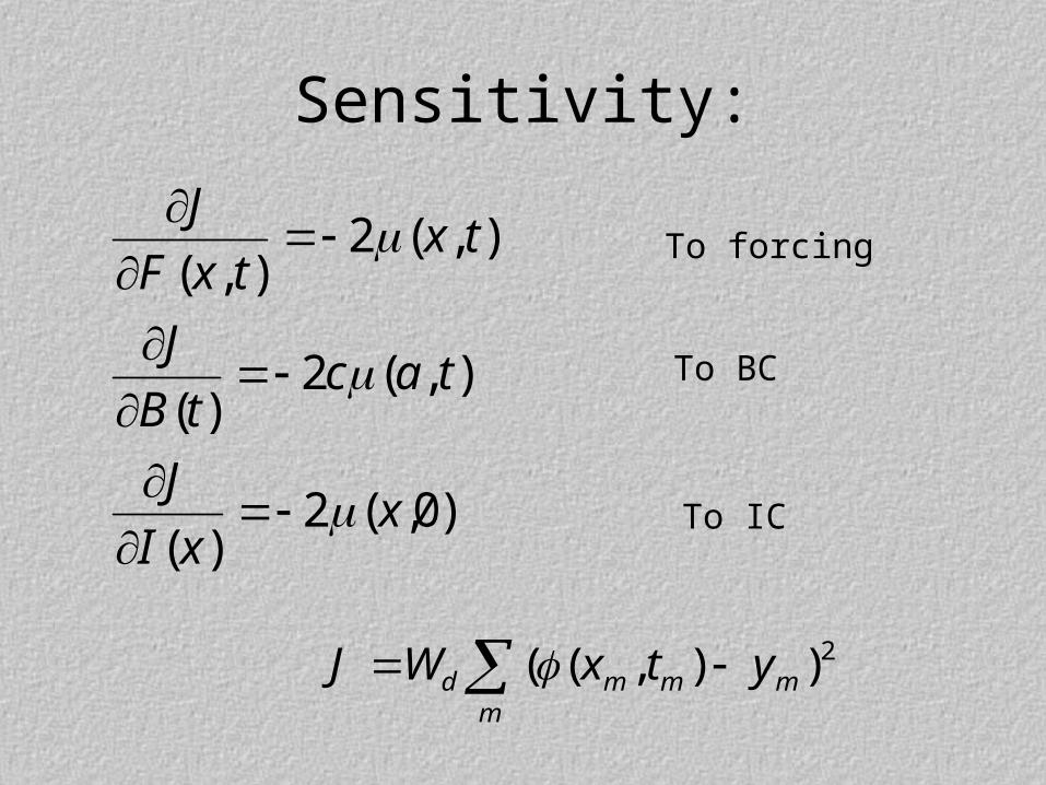
Also sensitivity:

To forcing

To BC

To IC)0,(2)(

),(2)(

),(2),(

xxI

J

tactB

J

txtxF

J

m

mmmd

T

b

b

a

if ytxWdtbWdxiWdxdtfWJ 2

0

222 )),((

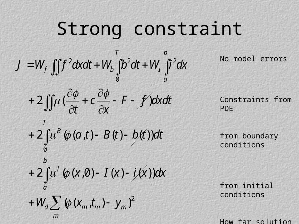
Strong constraint

2 2 2

0

0

2

2 ( )

2 ( ( , ) ( ) ( ))

2 ( ( ,0) ( ) ( ))

( ( , ) )

T b

f b I

a

TB

bI

a

d m m mm

J W f dxdt W b dt W i dx

c F f dxdtt x

a t B t b t dt

x I x i x dx

W x t y

No model errors

Constraints from PDE

from boundary conditions

from initial conditions

How far solution is from to the data

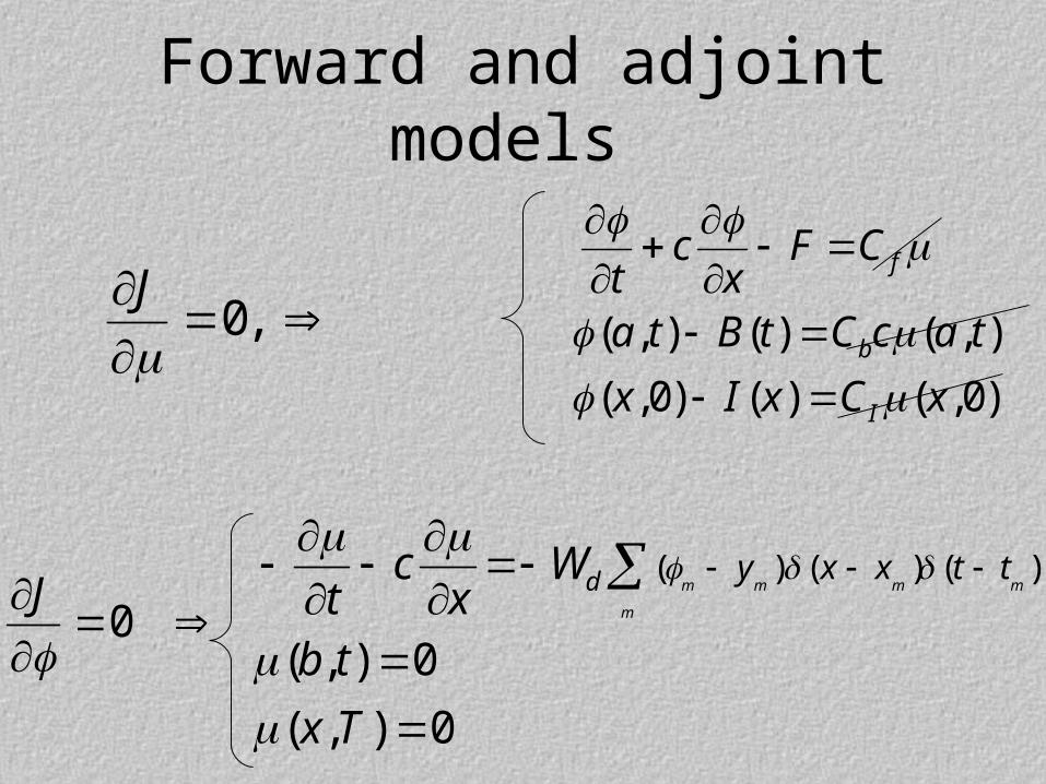
Forward and adjoint models

( , ) ( ) ( , )

( ,0) ( ) ( ,0)

f

b

I

c F Ct xa t B t C c a t

x I x C x

( ) ( ) ( )

( , ) 0

( , ) 0

m m m m

m

d y x x t tc Wt xb t

x T

,0J

0J

Sensitivity:

To forcing

To BC

To IC)0,(2)(

),(2)(

),(2),(

xxI

J

tactB

J

txtxF

J

m

mmmd ytxWJ 2)),((

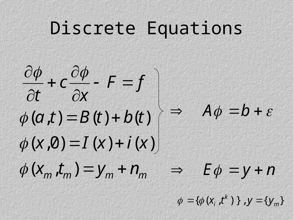
Discrete Equations

( , ) ( ) ( )

( ,0) ( ) ( )

( , )m m m m

c F ft xa t B t b t

x I x i x

x t y n

bA

nyE

}{)},,({ mk

i yytx

2 2 2

0

0

2

2 ( )

2 ( ( , ) ( ) ( ))

2 ( ( ,0) ( ) ( ))

( ( , ) )

T b

f b I

a

TB

bI

a

d m m mm

J W f dxdt W b dt W i dx

c F f dxdtt x

a t B t b t dt

x I x i x dx

W x t y

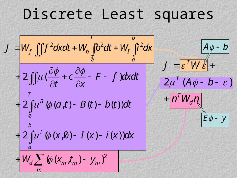
Discrete Least squares

nWn

bA

WJ

dT

T

T

)(2

bA

yE

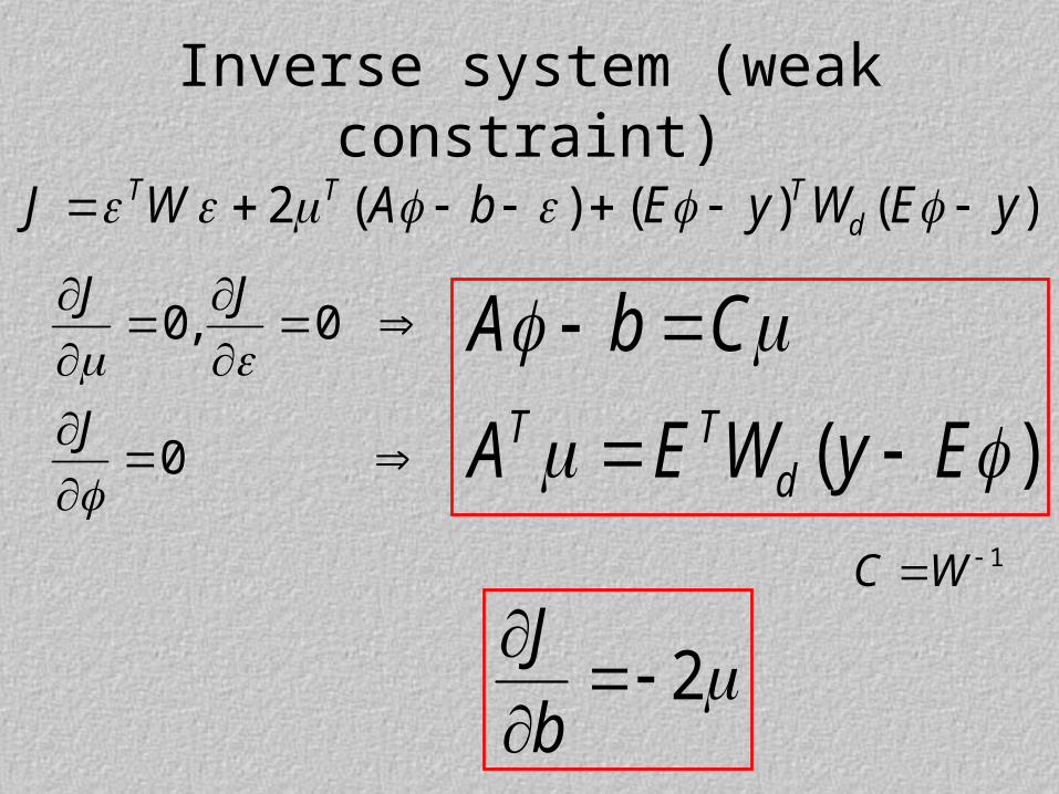
Inverse system (weak constraint)

)()()(2 yEWyEbAWJ dTTT

0

0,0

J

JJ

)(

EyWEA

CbA

dTT

2b

J1WC

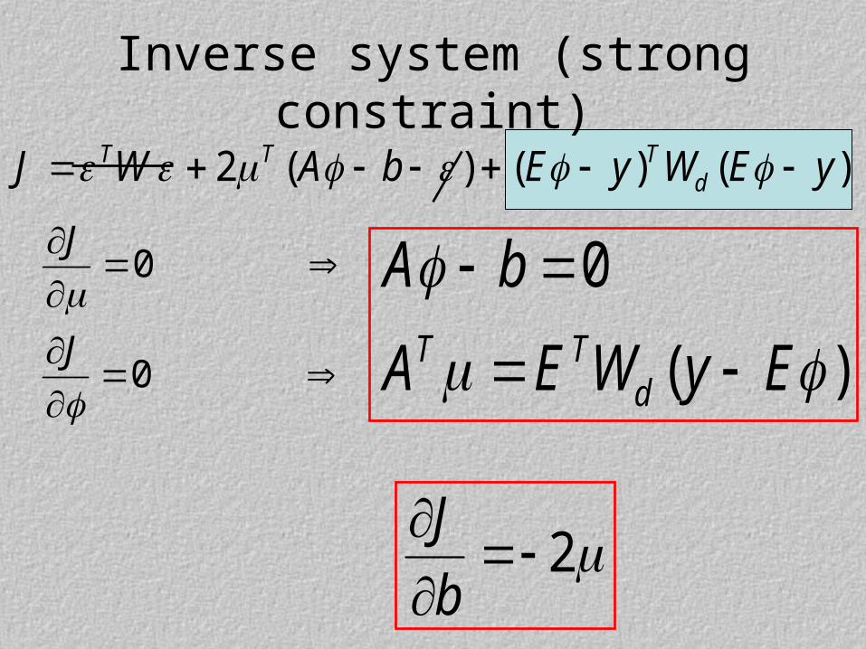
Inverse system (strong constraint)

)()()(2 yEWyEbAWJ dTTT

0

0

J

J

)(

0

EyWEA

bA

dTT

2b

J

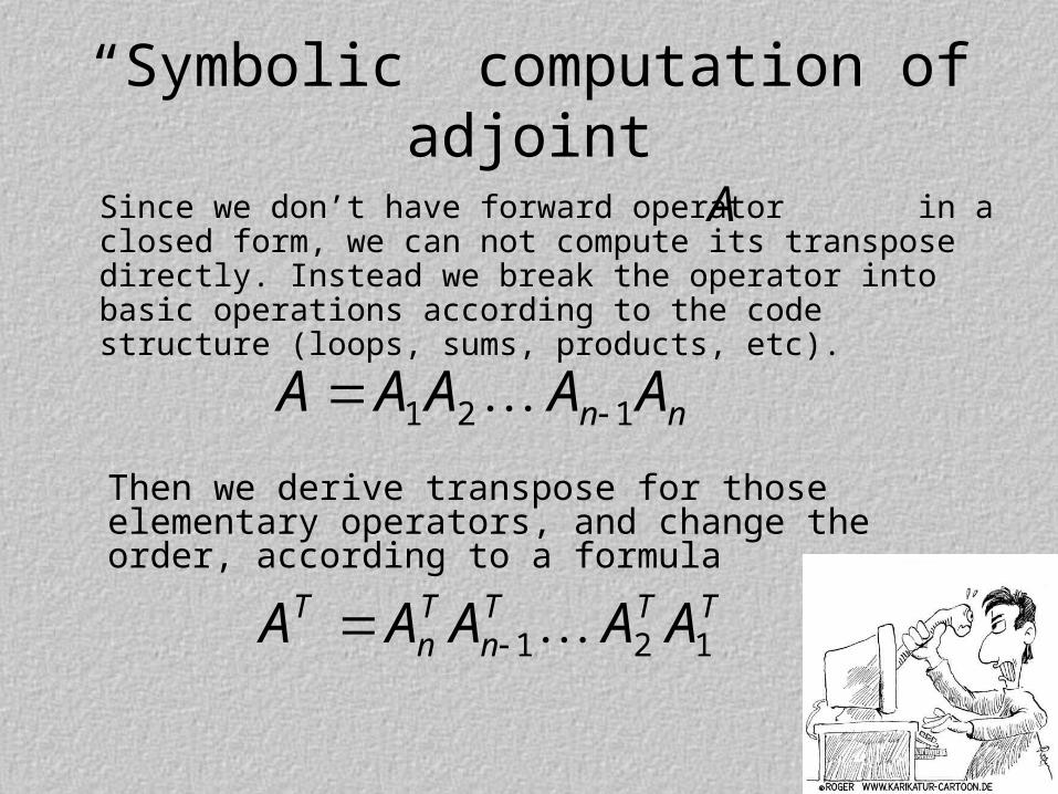
“Symbolic” computation of adjoint

Since we don’t have forward operator in a closed form, we can not compute its transpose directly. Instead we break the operator into basic operations according to the code structure (loops, sums, products, etc).

nn AAAAA 121

A

Then we derive transpose for those elementary operators, and change the order, according to a formula

TTTn

Tn

T AAAAA 121

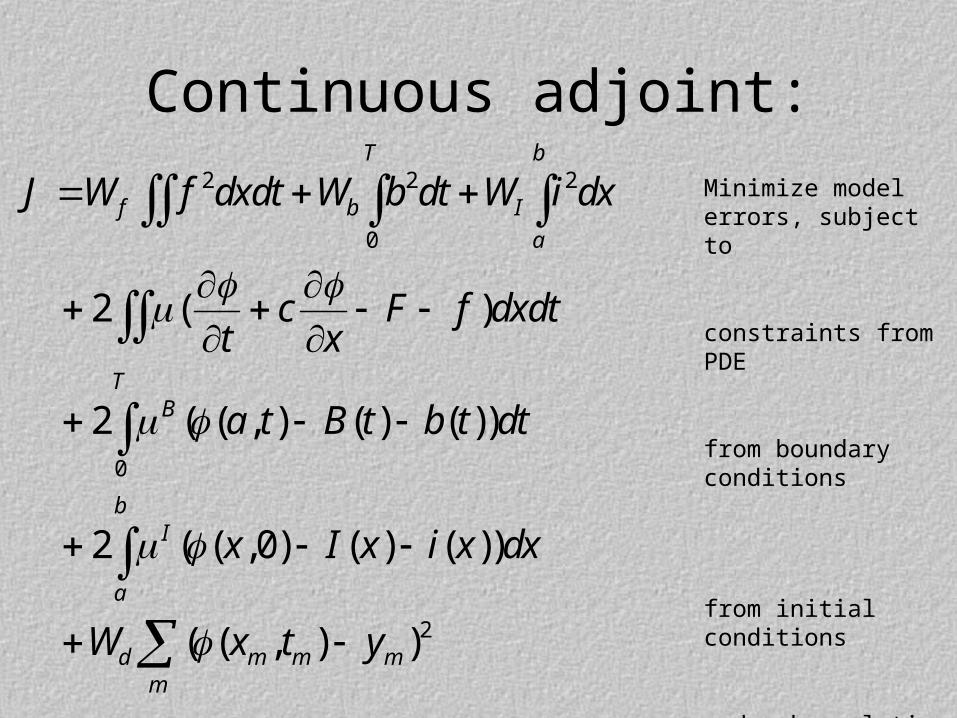
Continuous adjoint:2 2 2

0

0

2

2 ( )

2 ( ( , ) ( ) ( ))

2 ( ( ,0) ( ) ( ))

( ( , ) )

T b

f b I

a

TB

bI

a

d m m mm

J W f dxdt W b dt W i dx

c F f dxdtt x

a t B t b t dt

x I x i x dx

W x t y

Minimize model errors, subject to

constraints from PDE

from boundary conditions

from initial conditions

and make solution closest to the data

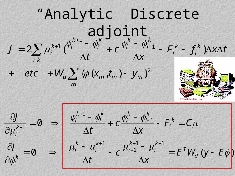
“Analytic” Discrete adjoint

mmmmd

ki

ki

ki

ki

ki

ki

kik

i

ytxWetc

txfFx

ct

J

2

1

,

11

)),((

)(2

)(0

0

111

1

11

1

EyWEx

ct

J

CFx

ct

J

dT

ki

ki

ki

ki

ki

ki

ki

ki

ki

ki

ki

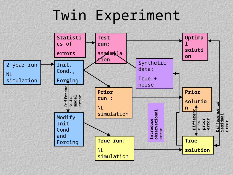
Twin Experiment

2 year run

NL simulation

Init. Cond.,

Forcing

True run:

NL simulation

True

solution

Modify Init Cond and Forcing

Dif

fere

nce

is

mod

el e

rror

Prior run :

NL simulation

Prior

solution

Synthetic data:

True + noise

Intr

odu

ce

obse

rvat

ion

al e

rror

Test run:

assimilation

Optimal solution

Statistics of

errors

Dif

fere

nce

is

resi

du

al e

rror

Dif

fere

nce

is

pri

or e

rror

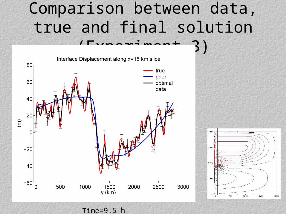
Comparison between data, true and final solution (Experiment 3)

Time=9.5 h

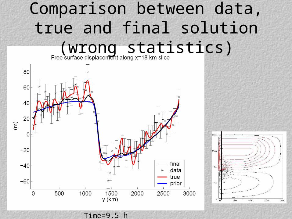
Comparison between data, true and final solution (wrong statistics)

Time=9.5 h

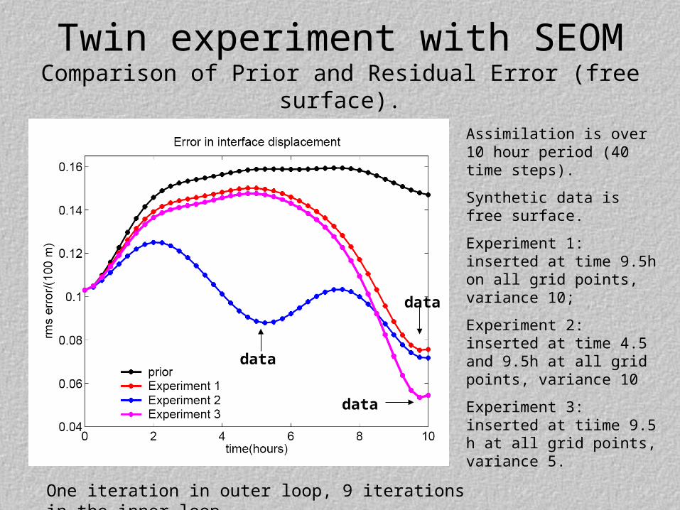
Twin experiment with SEOM Comparison of Prior and Residual Error (free surface).

Assimilation is over 10 hour period (40 time steps).

Synthetic data is free surface.

Experiment 1: inserted at time 9.5h on all grid points, variance 10;

Experiment 2: inserted at time 4.5 and 9.5h at all grid points, variance 10

Experiment 3: inserted at tiime 9.5 h at all grid points, variance 5.

data

data

data

One iteration in outer loop, 9 iterations in the inner loop

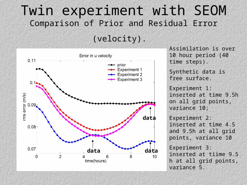
Twin experiment with SEOM Comparison of Prior and Residual Error (velocity).

data

data data

Assimilation is over 10 hour period (40 time steps).

Synthetic data is free surface.

Experiment 1: inserted at time 9.5h on all grid points, variance 10;

Experiment 2: inserted at time 4.5 and 9.5h at all grid points, variance 10

Experiment 3: inserted at tiime 9.5 h at all grid points, variance 5.

Conclusion

• “Symbolic” method is a powerful tool to build complex adjoint operators, but it produces a unintuitive code, and does not provide any insight on the resulting discrete adjoint equations, more difficult to debug and analize.

• Continuous adjoint equations are very important in understanding the adjoint processes. Usually, they are not difficult to derive.

• “Analytic”approach to building discrete adjoint equations provides good understanding of the numerics of an adjoint code; the adjoint code is more compact and more readable; but the equations can be difficult to derive, especially for complex difference schemes.