GEOPHYSICAL RESEARCH LETTERS, VOL. 40, 2557–2561, doi:10.1002/grl.50514, 2013

Observations of core-mantle boundary Stoneley modesPaula Koelemeijer,1 Arwen Deuss,1 and Jeroen Ritsema2

Received 11 March 2013; revised 22 April 2013; accepted 26 April 2013; published 4 June 2013.

[1] Core-mantle boundary (CMB) Stoneley modes repre-sent a unique class of normal modes with extremely strongsensitivity to wave speed and density variations in theD” region. We measure splitting functions of eight CMBStoneley modes using modal spectra from 93 events withMw > 7.4 between 1976 and 2011. The obtained splittingfunction maps correlate well with the predicted splittingcalculated for S20RTS+Crust5.1 structure and the distri-bution of Sdiff and Pdiff travel time anomalies, suggestingthat they are robust. We illustrate how our new CMBStoneley mode splitting functions can be used to estimatedensity variations in the Earth’s lowermost mantle. Citation:Koelemeijer, P., A. Deuss, and J. Ritsema (2013), Observationsof core-mantle boundary Stoneley modes, Geophys. Res. Lett., 40,2557–2561, doi:10.1002/grl.50514.

1. Introduction[2] The D” region is the lowest 200–300 km of the mantle,

atop the core-mantle boundary (CMB). D” is characterizedby ultra-low-velocity zones (ULVZs), seismic disconti-nuities, anisotropy, CMB topography, and, most promi-nently, by large-low-shear-velocity provinces (LLSVPs)below Africa and the Pacific [e.g., Lay, 2007; Garnero andMcNamara, 2008]. The LLSVPs extend hundreds of kilo-meters both laterally and vertically into the lower mantle[Ritsema et al., 1999]. To assess their effect on mantledynamics, it is essential to have information on the densityvariations [Forte and Mitrovica, 2001].

[3] Observations of Earth’s normal modes have the poten-tial to constrain both wave speed and density variations inthe mantle. Previous normal mode analyses suggest an anti-correlation between variations in the seismic shear veloc-ity and density, particularly for the LLSVPs [e.g., Ishiiand Tromp, 1999; Trampert et al., 2004; Mosca et al.,2012]. These results motivated the modeling of LLSVPsas long-lived “piles” of intrinsically dense material [e.g.,Davaille, 1999; McNamara and Zhong, 2005]. However,it was debated whether some of these density models arerobust, as they depend on the regularization and a priori con-straints [Romanowicz, 2001; Kuo and Romanowicz, 2002],and the studied modes have sensitivity to both the upper andlower mantle [Resovsky and Ritzwoller, 1999].

Additional supporting information may be found in the online versionof this article.

1Bullard Laboratories, University of Cambridge, Cambridge, UK.2Department of Earth and Environmental Sciences, University of

Michigan, Ann Arbor, Michigan, USA.

Corresponding author: P. J. Koelemeijer, Bullard Laboratories,Department of Earth Sciences, University of Cambridge, Madingley Rise,Madingley Road, Cambridge, CB3 0EZ, UK. (pjk49@cam.ac.uk)

©2013. American Geophysical Union. All Rights Reserved.0094-8276/13/10.1002/grl.50514

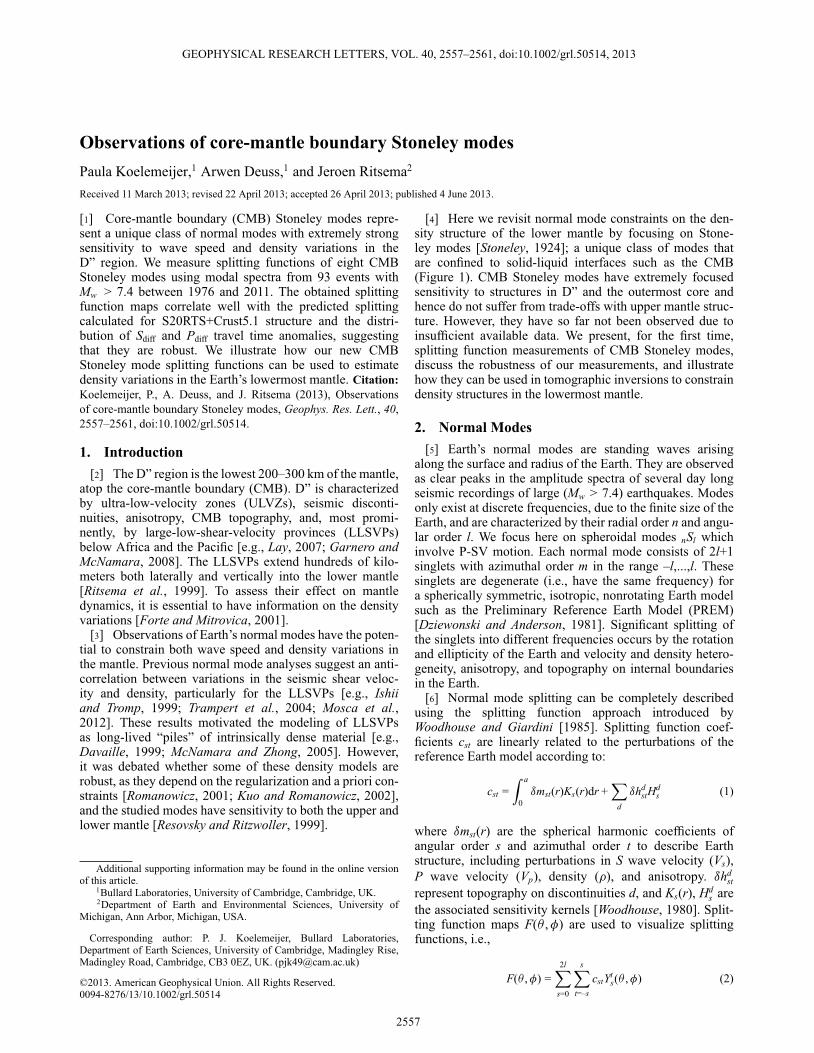
[4] Here we revisit normal mode constraints on the den-sity structure of the lower mantle by focusing on Stone-ley modes [Stoneley, 1924]; a unique class of modes thatare confined to solid-liquid interfaces such as the CMB(Figure 1). CMB Stoneley modes have extremely focusedsensitivity to structures in D” and the outermost core andhence do not suffer from trade-offs with upper mantle struc-ture. However, they have so far not been observed due toinsufficient available data. We present, for the first time,splitting function measurements of CMB Stoneley modes,discuss the robustness of our measurements, and illustratehow they can be used in tomographic inversions to constraindensity structures in the lowermost mantle.

2. Normal Modes[5] Earth’s normal modes are standing waves arising

along the surface and radius of the Earth. They are observedas clear peaks in the amplitude spectra of several day longseismic recordings of large (Mw > 7.4) earthquakes. Modesonly exist at discrete frequencies, due to the finite size of theEarth, and are characterized by their radial order n and angu-lar order l. We focus here on spheroidal modes nSl whichinvolve P-SV motion. Each normal mode consists of 2l+1singlets with azimuthal order m in the range –l,...,l. Thesesinglets are degenerate (i.e., have the same frequency) fora spherically symmetric, isotropic, nonrotating Earth modelsuch as the Preliminary Reference Earth Model (PREM)[Dziewonski and Anderson, 1981]. Significant splitting ofthe singlets into different frequencies occurs by the rotationand ellipticity of the Earth and velocity and density hetero-geneity, anisotropy, and topography on internal boundariesin the Earth.

[6] Normal mode splitting can be completely describedusing the splitting function approach introduced byWoodhouse and Giardini [1985]. Splitting function coef-ficients cst are linearly related to the perturbations of thereference Earth model according to:

cst =Z a

0ımst(r)Ks(r)dr +

Xd

ıhdstH

ds (1)

where ımst(r) are the spherical harmonic coefficients ofangular order s and azimuthal order t to describe Earthstructure, including perturbations in S wave velocity (Vs),P wave velocity (Vp), density (�), and anisotropy. ıhd

strepresent topography on discontinuities d, and Ks(r), Hd

s arethe associated sensitivity kernels [Woodhouse, 1980]. Split-ting function maps F(� ,�) are used to visualize splittingfunctions, i.e.,

F(� ,�) =2lX

s=0

sXt=–s

cstYts(� ,�) (2)

2557

KOELEMEIJER ET AL.: CMB STONELEY MODE SPLITTING FUNCTIONS

(a) 1S12

Surface

CMB

D’’

(b) 2S16 (c) 3S26

CMB

100km

D’’

Vp sensitivity Vs sensitivity sensitivity

Figure 1. Sensitivity kernels for Vp (solid), Vs (dashed),and � (red) for representative CMB Stoneley modes nSl anda zoom of the sensitivity in the D” region. Note that theStoneley mode sensitivity becomes more focused at theCMB with increasing angular order l.

where Yts(� ,�) are the complex spherical harmonics of

Edmonds [1960]. These maps show the local variation insplitting due to the underlying heterogeneity.

3. Methods and Data[7] Splitting functions are measured from the inversion of

spectra observed for large earthquakes. We make use of arecent normal mode spectra data set of 92 events with Mw >7.4 for the period 1976–2011 [Deuss et al., 2011, 2013], withthe addition of the 2011 Tohoku event (Mw = 9.0). FollowingDeuss et al. [2013], we measure the splitting functions usingnonlinear iterative least squares inversion [Tarantola andValette, 1982], starting from PREM or predictions for man-tle and crust structure. Cross validation is used to determinethe errors of our measured coefficients.

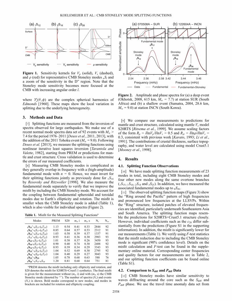
[8] Measuring CMB Stoneley modes is complicated asthey generally overlap in frequency with a (high-amplitude)fundamental mode with n = 0. Hence, we must invert fortheir splitting functions jointly as previously done for 1S14by Resovsky and Ritzwoller [1998]. We also measure thefundamental mode separately to verify that we improve themisfit by including the CMB Stoneley mode. We account forthe coupling between fundamental spheroidal and toroidalmodes due to Earth’s ellipticity and rotation. The misfit issmaller when the CMB Stoneley mode is added (Table 1),which is also visible for individual spectra (Figure 2).

Table 1. Misfit for the Measured Splitting Functionsa

Modes PREM S20 mst i mst s Ns Nev

1S11s-0S15-(0T16) 1.13 0.54 0.41 0.33 2844 92

1S12s-0S17-(0T18) 0.85 0.64 0.57 0.53 2312 91

1S13s-0S19-(0T20) 1.03 0.58 0.39 0.37 1337 91

1S14s-0S21-(0T22) 0.93 0.41 0.36 0.30 2983 93

1S15-0S23-(0T24) 1.01 0.38 0.37 0.26 3450 931S16-0S25-(0T26) 0.90 0.40 0.74 0.30 2488 922S14-0S22-(0T23) 0.93 0.39 0.34 0.29 3343 932S15

s-0S24-(0T25) 1.04 0.52 0.69 0.30 2795 922S16

s-0S26-(0T27) 1.04 0.40 0.29 0.27 3043 932S25

s-3S25 1.05 0.78 0.68 0.63 588 763S26

s-6S15-9S10 1.20 0.81 0.68 0.64 751 81

aPREM denotes the misfit including only ellipticity and rotation, andS20 denotes the misfit for S20RTS+Crust5.1 synthetics. The final misfitis given for the measurement without (mst i) and with (mst s) the CMBStoneley mode (denoted by ‘s’). The number of spectra (Ns) and events(Ne) is shown. Bold modes correspond to new modes, and modes inbrackets are included for rotation and ellipticity coupling.

0

Nor

mal

ised

am

plitu

de

2.54 2.56 2.58

Frequency (mHz)

Fundamental mode0S17

Stoneleymode1S12

0

Pha

se

(a) 070508A − SUR

3.42 3.44 3.46

Frequency (mHz)

Fundamentalmode

0S26

Stoneleymode2S16

(b) 122604A − INCN

Data Fundamental Fundamental+Stoneley

Figure 2. Amplitude and phase spectra for (a) a deep event(Okhotsk, 2008, 615 km, Mw = 7.7) at station SUR (SouthAfrica) and (b) a shallow event (Sumatra, 2004, 28.6 km,Mw = 9.0) at station INCN (South Korea).

[9] We compare our measurements to predictions formantle and crust structure, calculated using mantle Vs modelS20RTS [Ritsema et al., 1999]. We assume scaling factorsof the form Rp = ılnVp/ılnVs = 0.5 and R� = ıln�/ılnVs =0.3, consistent with previous work [Karato, 1993; Li et al.,1991]. The contributions of crustal thickness, surface topog-raphy, and water level are calculated using model Crust5.1[Mooney et al., 1998].

4. Results4.1. Splitting Function Observations

[10] We have made splitting function measurements of 23modes in total, including eight CMB Stoneley modes andfour other new modes along the same overtone branches(1S15, 1S16, 2S14 and 3S25). In addition, we have measured theassociated fundamental modes up to 0S26.

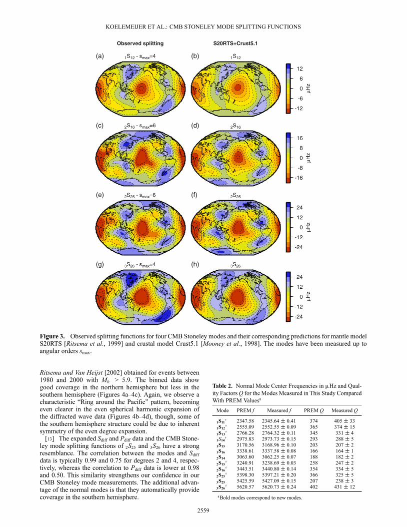
[11] The observed splitting function maps (Figure 3) showthe “Ring around the Pacific” pattern of high frequenciesand pronounced low frequencies at the LLSVPs. Withinthe “Ring” structure, isolated patches of elevated frequen-cies are identified, particularly underneath Southeastern Asiaand South America. The splitting function maps resem-ble the predictions for S20RTS+Crust5.1 structure closely.However, individual coefficients such as the c20 differ sub-stantially from the predictions (Figure S1 in the supportinginformation). In addition, the misfit is significantly lower forour measurements (Table 1). We verify using F-test statisticsthat the misfit reduction due to including the CMB Stoneleymode is significant (90% confidence level). Details on themisfit calculation and F-test can be found in the supple-mentary online material. Corresponding center frequenciesand quality factors for our measurements are in Table 2,and our splitting function coefficients can be found online(Table S1).

4.2. Comparison to Sdiff and Pdiff Data[12] CMB Stoneley modes have similar sensitivity to

waves diffracting around the core such as the Sdiff andPdiff phase. We use the travel time anomaly data set from

2558

KOELEMEIJER ET AL.: CMB STONELEY MODE SPLITTING FUNCTIONS

Observed splitting

(a) 1S12 - smax=4

2S25 - smax=6

3S26 - smax=4

2S16 - smax=6

S20RTS+Crust5.1

(b) 1S12

2S16

2S25

3S26

-12

-6

0

6

12

μHz

μHz

μHz

μHz

(c) (d)

-16

-8

0

8

16

(e) (f)

-24

-12

0

12

24

(g) (h)

-24

-12

0

12

24

Figure 3. Observed splitting functions for four CMB Stoneley modes and their corresponding predictions for mantle modelS20RTS [Ritsema et al., 1999] and crustal model Crust5.1 [Mooney et al., 1998]. The modes have been measured up toangular orders smax.

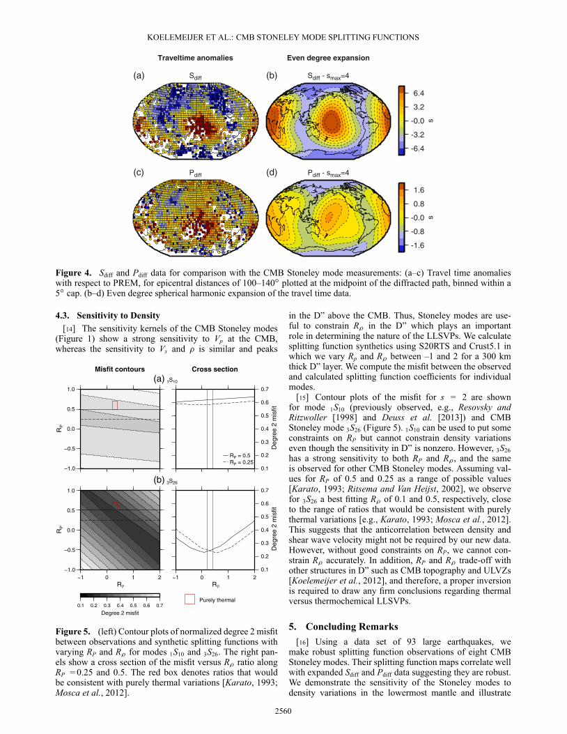
Ritsema and Van Heijst [2002] obtained for events between1980 and 2000 with Mb > 5.9. The binned data showgood coverage in the northern hemisphere but less in thesouthern hemisphere (Figures 4a–4c). Again, we observe acharacteristic “Ring around the Pacific” pattern, becomingeven clearer in the even spherical harmonic expansion ofthe diffracted wave data (Figures 4b–4d), though, some ofthe southern hemisphere structure could be due to inherentsymmetry of the even degree expansion.

[13] The expanded Sdiff and Pdiff data and the CMB Stone-ley mode splitting functions of 2S25 and 3S26 have a strongresemblance. The correlation between the modes and Sdiffdata is typically 0.99 and 0.75 for degrees 2 and 4, respec-tively, whereas the correlation to Pdiff data is lower at 0.98and 0.50. This similarity strengthens our confidence in ourCMB Stoneley mode measurements. The additional advan-tage of the normal modes is that they automatically providecoverage in the southern hemisphere.

Table 2. Normal Mode Center Frequencies in �Hz and Qual-ity Factors Q for the Modes Measured in This Study ComparedWith PREM Valuesa

Mode PREM f Measured f PREM Q Measured Q

1S11s 2347.58 2345.64˙ 0.41 374 405˙ 33

1S12s 2555.09 2552.55˙ 0.09 365 374˙ 15

1S13s 2766.28 2764.32˙ 0.11 345 331˙ 4

1S14s 2975.83 2973.73˙ 0.15 293 288˙ 5

1S15 3170.56 3168.96˙ 0.10 203 207˙ 21S16 3338.61 3337.58˙ 0.08 166 164˙ 12S14 3063.60 3062.25˙ 0.07 188 182˙ 22S15

s 3240.91 3238.69˙ 0.03 258 247˙ 22S16

s 3443.51 3440.80˙ 0.14 354 334˙ 52S25

s 5398.30 5397.21˙ 0.20 366 325˙ 53S25 5425.59 5427.09˙ 0.15 207 238˙ 33S26

s 5620.57 5620.73˙ 0.24 402 431˙ 12

aBold modes correspond to new modes.

2559

KOELEMEIJER ET AL.: CMB STONELEY MODE SPLITTING FUNCTIONS

Traveltime anomalies

(a) Sdiff

Pdiff

Even degree expansion

(b) Sdiff - smax=4

Pdiff - smax=4

-6.4

-3.2

-0.0

3.2

6.4

s

(c) (d)

-1.6

-0.8

-0.0

0.8

1.6

s

Figure 4. Sdiff and Pdiff data for comparison with the CMB Stoneley mode measurements: (a–c) Travel time anomalieswith respect to PREM, for epicentral distances of 100–140ı plotted at the midpoint of the diffracted path, binned within a5ı cap. (b–d) Even degree spherical harmonic expansion of the travel time data.

4.3. Sensitivity to Density[14] The sensitivity kernels of the CMB Stoneley modes

(Figure 1) show a strong sensitivity to Vp at the CMB,whereas the sensitivity to Vs and � is similar and peaks

−1.0

−0.5

0.0

0.5

1.0

−1.0

−0.5

0.0

0.5

1.0

−1 0 1 2

0.1 0.2 0.3 0.4 0.5 0.6 0.7

Degree 2 misfit

0.1

0.2

0.3

0.4

0.5

0.6

0.7

0.1

0.2

0.3

0.4

0.5

0.6

0.7

Deg

ree

2 m

isfit

RP = 0.5RP = 0.25

Deg

ree

2 m

isfit

−1 0 1 2

RP

RP

RρRρ

Purely thermal

(b) 3S26

(a) 1S10

Misfit contours Cross section

Figure 5. (left) Contour plots of normalized degree 2 misfitbetween observations and synthetic splitting functions withvarying RP and R� for modes 1S10 and 3S26. The right pan-els show a cross section of the misfit versus R� ratio alongRP = 0.25 and 0.5. The red box denotes ratios that wouldbe consistent with purely thermal variations [Karato, 1993;Mosca et al., 2012].

in the D” above the CMB. Thus, Stoneley modes are use-ful to constrain R� in the D” which plays an importantrole in determining the nature of the LLSVPs. We calculatesplitting function synthetics using S20RTS and Crust5.1 inwhich we vary Rp and R� between –1 and 2 for a 300 kmthick D” layer. We compute the misfit between the observedand calculated splitting function coefficients for individualmodes.

[15] Contour plots of the misfit for s = 2 are shownfor mode 1S10 (previously observed, e.g., Resovsky andRitzwoller [1998] and Deuss et al. [2013]) and CMBStoneley mode 3S26 (Figure 5). 1S10 can be used to put someconstraints on RP but cannot constrain density variationseven though the sensitivity in D” is nonzero. However, 3S26has a strong sensitivity to both RP and R�, and the sameis observed for other CMB Stoneley modes. Assuming val-ues for RP of 0.5 and 0.25 as a range of possible values[Karato, 1993; Ritsema and Van Heijst, 2002], we observefor 3S26 a best fitting R� of 0.1 and 0.5, respectively, closeto the range of ratios that would be consistent with purelythermal variations [e.g., Karato, 1993; Mosca et al., 2012].This suggests that the anticorrelation between density andshear wave velocity might not be required by our new data.However, without good constraints on RP, we cannot con-strain R� accurately. In addition, RP and R� trade-off withother structures in D” such as CMB topography and ULVZs[Koelemeijer et al., 2012], and therefore, a proper inversionis required to draw any firm conclusions regarding thermalversus thermochemical LLSVPs.

5. Concluding Remarks[16] Using a data set of 93 large earthquakes, we

make robust splitting function observations of eight CMBStoneley modes. Their splitting function maps correlate wellwith expanded Sdiff and Pdiff data suggesting they are robust.We demonstrate the sensitivity of the Stoneley modes todensity variations in the lowermost mantle and illustrate

2560

KOELEMEIJER ET AL.: CMB STONELEY MODE SPLITTING FUNCTIONS

the trade-off with P wave velocity structure. This trade-offcan be partially removed when we consider thinner layers(100 km thick) due to the nature of the sensitivity kernels(Figure 1). In addition, a large number of P wave sensi-tive normal mode observations is available [Deuss et al.,2013], and body wave data also provide constraints onRP. Therefore, when our new measurements are includedwith these in tomographic inversions, they will help toprovide tighter constraints on the density variations in thelowermost mantle.

[17] Acknowledgments. We thank the Editor (Michael Wyssession),Caroline Beghein, and Joseph Resovsky for their detailed comments, whichgreatly improved the manuscript. Data were provided by the IRIS/DMC.PJK and AD are funded by the European Research Council under theEuropean Community’s 7th Framework Programme (FP7/2007-2013)/ERCgrant agreement 204995. PJK is also supported by the Nahum Scholarshipin Physics and a Graduate Studentship, both from Pembroke College,Cambridge. AD is also funded by a Philip Leverhulme Prize, and JR is sup-ported by NSF grant EAR-1014749. We would like to thank Anna Mäkinenfor advice on the F-test statistics. Figures have been produced using theGMT software [Wessel and Smith, 1998].

[18] The Editor thanks Caroline Beghein and an anonymous reviewerfor their assistance in evaluating this paper.

ReferencesDavaille, A. (1999), Simultaneous generation of hotspots and superswells

by convection in a heterogeneous planetary mantle, Nature, 402(6763),756–760.

Deuss, A., J. Ritsema, and H. van Heijst (2011), Splitting function measure-ments for Earth’s longest period normal modes using recent large earth-quakes, Geophys. Res. Lett., 38, L04303, doi:10.1029/2010GL046115.

Deuss, A., J. Ritsema, and H. Van Heijst (2013), A new catalogue ofnormal-mode splitting function measurements up to 10 mHz, Geophys.J. Int., 193(2), 920–937, doi:10.1093/gji/ggt010.

Dziewonski, A., and D. Anderson (1981), Preliminary reference Earthmodel, Phys. Earth Planet. Inter., 25(4), 297–356.

Edmonds, A. (1960), Angular Momentum in Quantum Mechanics,Princeton University Press, Princeton, NJ.

Forte, A., and J. Mitrovica (2001), Deep-mantle high-viscosity flow andthermochemical structure inferred from seismic and geodynamic data,Nature, 410(6832), 1049–1056.

Garnero, E., and A. McNamara (2008), Structure and dynamics of Earth’slower mantle, Science, 320(5876), 626.

Ishii, M., and J. Tromp (1999), Normal-mode and free-air gravity con-straints on lateral variations in velocity and density of Earth’s mantle,Science, 285(5431), 1231.

Karato, S. (1993), Importance of anelasticity in the interpretation of seismictomography, Geophys. Res. Lett., 20(15), 1623–1626.

Koelemeijer, P., A. Deuss, and J. Trampert (2012), Normal mode sensitivityto Earth’s D” layer and topography on the core–mantle boundary: Whatwe can and cannot see, Geophys. J. Int., 190, 553–568.

Kuo, C., and B. Romanowicz (2002), On the resolution of density anomaliesin the Earth’s mantle using spectral fitting of normal-mode data, Geophys.J. Int., 150(1), 162–179.

Lay, T. (2007), Deep Earth structure – Lower mantle and D”, Treatise onGeophysics, 1, 620–654.

Li, X., D. Giardini, and J. Woodhouse (1991), The relative amplitudesof mantle heterogeneity in P velocity, S velocity and density fromfree-oscillation data, Geophys. J. Int., 105(3), 649–657.

McNamara, A. K., and S. Zhong (2005), Thermochemical structuresbeneath Africa and the Pacific Ocean, Nature, 437(7062), 1136–1139.

Mooney, W., G. Laske, and T. Masters (1998), CRUST 5.1: A global crustalmodel at 5� 5 ı, J. Geophys. Res., 103(B1), 727–747.

Mosca, I., L. Cobden, A. Deuss, J. Ritsema, and J. Trampert (2012),Seismic and mineralogical structures of the lower mantle from prob-abilistic tomography, J. Geophys. Res., 117, B06304, doi:10.1029/2011JB008851.

Resovsky, J., and M. Ritzwoller (1999), Regularization uncertainty in den-sity models estimated from normal mode data, Geophys. Res. Lett.,26(15), 2319–2322.

Resovsky, J. S., and M. H. Ritzwoller (1998), New and refined constraintson three-dimensional Earth structure from normal modes below 3 mHz,J. Geophys. Res., 103(B1), 783–810.

Ritsema, J., and H. Van Heijst (2002), Constraints on the correlation of P-and S-wave velocity heterogeneity in the mantle from P, PP, PPP andPKPab traveltimes, Geophys. J. Int., 149(2), 482–489.

Ritsema, J., H. Heijst, and J. Woodhouse (1999), Complex shearwave velocity structure imaged beneath Africa and Iceland, Science,286(5446), 1925.

Romanowicz, B. (2001), Can we resolve 3D density heterogeneity in thelower mantle? Geophys. Res. Lett., 28(6), 1107–1110.

Stoneley, R. (1924), Elastic waves at the surface of separation of two solids,Proc. R. Soc. London, Ser. A, Containing Papers of a Mathematical andPhysical Character, 106(738), 416–428.

Tarantola, A., and B. Valette (1982), Generalized nonlinear inverse prob-lems solved using the least squares criterion, Rev. Geophys. Space. Phys.,20(2), 219–232.

Trampert, J., F. Deschamps, J. Resovsky, and D. Yuen (2004), Probabilistictomography maps chemical heterogeneities throughout the lower mantle,Science, 306(5697), 853.

Wessel, P., and W. Smith (1998), New, improved version of the genericmapping tools released, Eos Trans. AGU, 79, 579–579.

Woodhouse, J. (1980), The coupling and attenuation of nearly resonant mul-tiplets in the Earth’s free oscillation spectrum, Geophys. J. R. Astr. Soc.,61(2), 261–283.

Woodhouse, J., and D. Giardini (1985), Inversion for the splitting functionof isolated low order normal mode multiplets, Eos Trans. AGU, 66, 300.

2561