objective functions for full waveform inversiontrip.rice.edu/downloads/talk_ws05.pdf · objective...
TRANSCRIPT
Objective functions for full waveform inversion
William Symes
The Rice Inversion Project
EAGE 2012Workshop: From Kinematic to Waveform Inversion
A Tribute to Patrick Lailly

Agenda
Overview
Challenges for FWI
Extended modeling
Summary
Full Waveform Inversion
M = model space, D = data space
F : M → D forward model
Least squares inversion (“FWI”): given d ∈ D, find m ∈ M tominimize
JLS [m] = ‖F [m]− d‖2[+ regularizing terms]
(‖ · ‖2 = mean square)
Full Waveform Inversion
+ accommodates any modeling physics, data geometry, spatialvariation on all scales (Bamberger, Chavent & Lailly 79,...)
+ close relation to prestack migration via local optimization(Lailly 83, Tarantola 84)
+ gains in hard/software, algorithm efficiency ⇒ feasible dataprocessing method
++ some spectacular successes with 3D field data (keep listening!)
± with regularizations pioneered by Pratt and others, applicablesurface data if sufficient (i) low frequency s/n and (ii) longoffsets
- reflection data still a challenge
Full Waveform Inversion
Why are
I low frequencies important?
I long offsets (diving waves, transmission) easier than shortoffsets (reflections)?
What alternatives to Standard FWI = output least squares?
I different error measures, domains - time vs. Fourier vs.Laplace, L1, logarithmic - other talks today, survey Virieux &Operto 09
I model extensions - migration velocity analysis as alinearization, nonlinear MVA

Agenda
Overview
Challenges for FWI
Extended modeling
Summary
Nonlinear Challenges: Why low frequencies are important
Well-established observation, based on heuristic arguments (“cycleskipping”), numerical evidence :forward modeling operator is morelinear [objective function is more quadratic] at lower frequencies
Leads to widely-used frequency continuation strategy (Kolb,Collino, & Lailly 86)
Why?
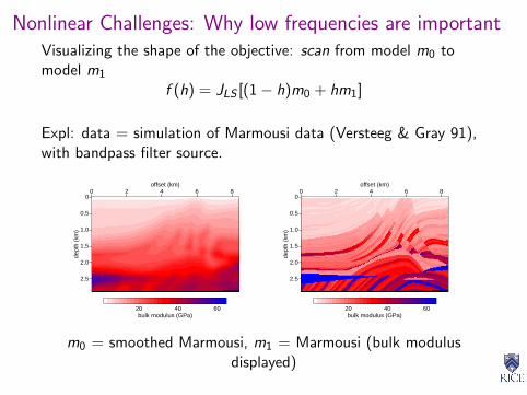
Nonlinear Challenges: Why low frequencies are importantVisualizing the shape of the objective: scan from model m0 tomodel m1
f (h) = JLS [(1− h)m0 + hm1]
Expl: data = simulation of Marmousi data (Versteeg & Gray 91),with bandpass filter source.
0
0.5
1.0
1.5
2.0
2.5
dept
h (k
m)
0 2 4 6 8offset (km)
20 40 60bulk modulus (GPa)
0
0.5
1.0
1.5
2.0
2.5de
pth
(km
)
0 2 4 6 8offset (km)
20 40 60bulk modulus (GPa)
m0 = smoothed Marmousi, m1 = Marmousi (bulk modulusdisplayed)
Nonlinear Challenges: Why low frequencies are important
0 0.2 0.4 0.6 0.8 1.0h (scan parameter)
0
0.5
1.0M
S e
rror
(no
rmal
ized
)
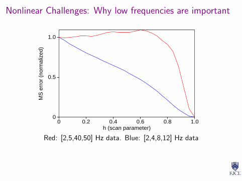
Red: [2,5,40,50] Hz data. Blue: [2,4,8,12] Hz data
Nonlinear Challenges: Why low frequencies are important
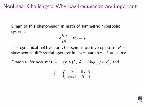
Origin of this phenomenon in math of symmetric hyperbolicsystems:
A∂u
∂t+ Pu = f
u = dynamical field vector, A = symm. positive operator, P =skew-symm. differential operator in space variables, f = source
Example: for acoustics, u = (p, v)T , A = diag(1/κ, ρ), and
P =
(0 div
grad 0
)
Nonlinear Challenges: Why low frequencies are important
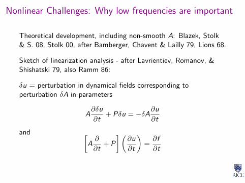
Theoretical development, including non-smooth A: Blazek, Stolk& S. 08, Stolk 00, after Bamberger, Chavent & Lailly 79, Lions 68.
Sketch of linearization analysis - after Lavrientiev, Romanov, &Shishatski 79, also Ramm 86:
δu = perturbation in dynamical fields corresponding toperturbation δA in parameters
A∂δu
∂t+ Pδu = −δA
∂u
∂t
and [A∂
∂t+ P
](∂u
∂t
)=∂f
∂t
Nonlinear Challenges: Why low frequencies are important
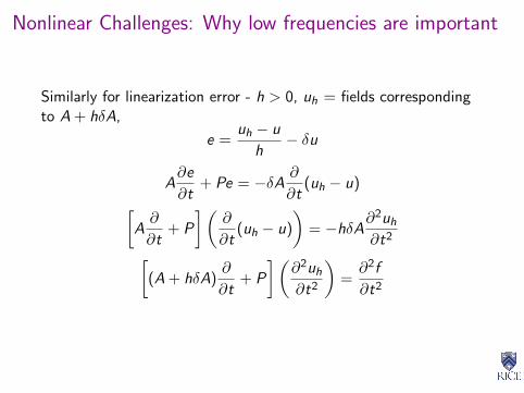
Similarly for linearization error - h > 0, uh = fields correspondingto A + hδA,
e =uh − u
h− δu
A∂e
∂t+ Pe = −δA
∂
∂t(uh − u)[
A∂
∂t+ P
](∂
∂t(uh − u)
)= −hδA
∂2uh
∂t2[(A + hδA)
∂
∂t+ P
](∂2uh
∂t2
)=∂2f
∂t2
Nonlinear Challenges: Why low frequencies are important
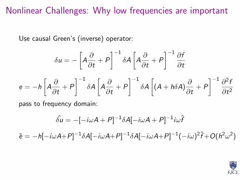
Use causal Green’s (inverse) operator:
δu = −[
A∂
∂t+ P
]−1
δA
[A∂
∂t+ P
]−1 ∂f
∂t
e = −h
[A∂
∂t+ P
]−1
δA
[A∂
∂t+ P
]−1
δA
[(A + hδA)
∂
∂t+ P
]−1 ∂2f
∂t2
pass to frequency domain:
δu = −[−iωA + P]−1δA[−iωA + P]−1iωf
e = −h[−iωA+P]−1δA[−iωA+P]−1δA[−iωA+P]−1(−iω)2f +O(h2ω2)
Nonlinear Challenges: Why low frequencies are important
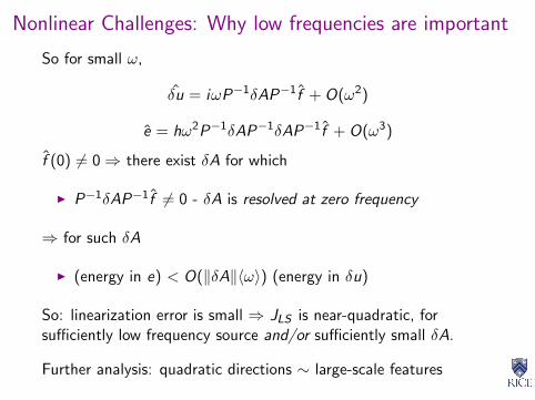
So for small ω,
δu = iωP−1δAP−1f + O(ω2)
e = hω2P−1δAP−1δAP−1f + O(ω3)
f (0) 6= 0⇒ there exist δA for which
I P−1δAP−1f 6= 0 - δA is resolved at zero frequency
⇒ for such δA
I (energy in e) < O(‖δA‖〈ω〉) (energy in δu)
So: linearization error is small ⇒ JLS is near-quadratic, forsufficiently low frequency source and/or sufficiently small δA.
Further analysis: quadratic directions ∼ large-scale features
Linear Challenges: Why reflection is hard
Relative difficulty of reflection vs. transmission
I numerical examples: Gauthier, Virieux & Tarantola 86
I spectral analysis of layered traveltime tomography: Baek &Demanet 11
Spectral analysis of reflection per se: Virieux & Operto 09
Linear Challenges: Why reflection is hard
Reproduction of “Camembert” Example (GVT 86) (thanks: DongSun)
Circular high-velocity zone in 1km × 1km square background - 2%∆v .
Transmission configuration: 8 sources at corners and sidemidpoints, 400 receivers (100 per side) surround anomaly.
Reflection configuration: all 8 sources, 100 receivers on one side(“top”).
Modeling details: 50 Hz Ricker source pulse, density fixed andconstant, staggered grid FD modeling, absorbing boundaries.
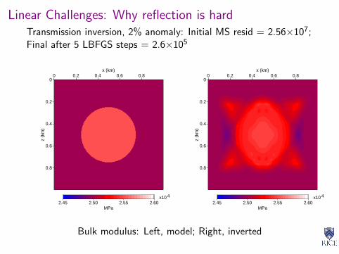
Linear Challenges: Why reflection is hardTransmission inversion, 2% anomaly: Initial MS resid = 2.56×10⁷;Final after 5 LBFGS steps = 2.6×10⁵
0
0.2
0.4
0.6
0.8
z (k
m)
0 0.2 0.4 0.6 0.8x (km)
2.45 2.50 2.55 2.60x10⁴
MPa
0
0.2
0.4
0.6
0.8
z (k
m)
0 0.2 0.4 0.6 0.8x (km)
2.45 2.50 2.55 2.60x10⁴
MPa
Bulk modulus: Left, model; Right, inverted
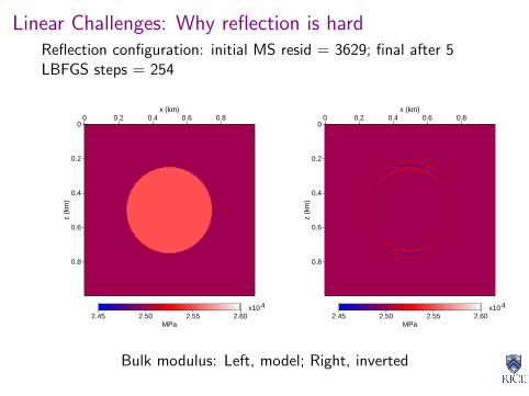
Linear Challenges: Why reflection is hardReflection configuration: initial MS resid = 3629; final after 5LBFGS steps = 254
0
0.2
0.4
0.6
0.8
z (k
m)
0 0.2 0.4 0.6 0.8x (km)
2.45 2.50 2.55 2.60x10⁴
MPa
0
0.2
0.4
0.6
0.8
z (k
m)
0 0.2 0.4 0.6 0.8x (km)
2.45 2.50 2.55 2.60x10⁴
MPa
Bulk modulus: Left, model; Right, inverted
Linear Challenges: Why reflection is hard
Message: in reflection case, “the Camembert has melted”.
Small anomaly ⇒ linear phenomenon
Linear resolution analysis (eg. Virieux & Operto 09): narrowaperture data does not resolve low spatial wavenumbers
Resolution analysis of phase (traveltime tomography) in layeredcase: Baek & Demanet 11
I model 7→ traveltime map = composition of (i) increasingrearangement, (ii) invertible algebraic tranformation, (iii)linear operator
I factor (iii) has singular values decaying like n−1/2 for divingwave traveltimes, expontially decaying for reflected wavetraveltimes.
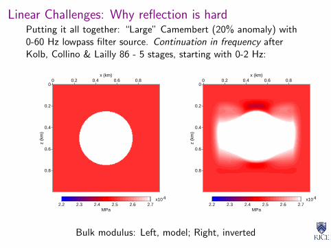
Linear Challenges: Why reflection is hardPutting it all together: “Large” Camembert (20% anomaly) with0-60 Hz lowpass filter source. Continuation in frequency afterKolb, Collino & Lailly 86 - 5 stages, starting with 0-2 Hz:
0
0.2
0.4
0.6
0.8
z (k
m)
0 0.2 0.4 0.6 0.8x (km)
2.2 2.3 2.4 2.5 2.6 2.7x10⁴
MPa
0
0.2
0.4
0.6
0.8
z (k
m)
0 0.2 0.4 0.6 0.8x (km)
2.2 2.3 2.4 2.5 2.6 2.7x10⁴
MPa
Bulk modulus: Left, model; Right, inverted

Agenda
Overview
Challenges for FWI
Extended modeling
Summary
Extended Models and Differential Semblance
Inversion of reflection data: difficulty rel. transmission is linear inorigin, so look to migration velocity analysis for useful ideas
Prestack migration as approximate inversion: fits subsets of datawith non-physical extended models (= image volume), so all datamatched - no serendipitous local matches!
Transfer info from small to large scales by demanding coherence ofextended models
Familiar concept from depth-domain migration velocity analysis -independent models (images) grouped together as image gathers,coherence ⇒ good velocity model
Exploit for automatic model estimation: residual moveout removal(Biondi & Sava 04, Biondi & Zhang 12), van Leeuwen & Mulder 08(data domain VA), differential waveform inversion (Chauris, postersession), differential semblance (image domain VA) S. 86 ...
Extended Models and Differential Semblance
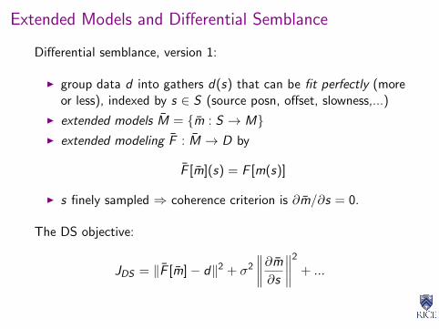
Differential semblance, version 1:
I group data d into gathers d(s) that can be fit perfectly (moreor less), indexed by s ∈ S (source posn, offset, slowness,...)
I extended models M = {m : S → M}I extended modeling F : M → D by
F [m](s) = F [m(s)]
I s finely sampled ⇒ coherence criterion is ∂m/∂s = 0.
The DS objective:
JDS = ‖F [m]− d‖2 + σ2
∥∥∥∥∂m
∂s
∥∥∥∥2
+ ...
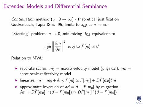
Extended Models and Differential Semblance
Continuation method (σ : 0→∞) - theoretical justificationGockenbach, Tapia & S. ’95, limits to JLS as σ →∞.
“Starting” problem: σ → 0, minimizing JDS equivalent to
minm
∥∥∥∥∂m
∂s
∥∥∥∥2
subj to F [m] ' d
Relation to MVA:
I separate scales: m0 = macro velocity model (physical), δm =short scale reflectivity model
I linearize: m = m0 + δm, F [m] ' F [m0] + DF [m0]δm
I approximate inversion of δd = d − F [m0] by migration:δm = DF [m0]−1(d − F [m0]) ' DF [m0]T (d − F [m0])
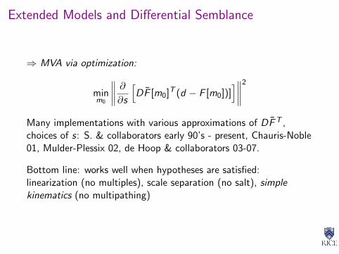
Extended Models and Differential Semblance
⇒ MVA via optimization:
minm0
∥∥∥∥ ∂∂s
[DF [m0]T (d − F [m0])]
]∥∥∥∥2
Many implementations with various approximations of DFT ,choices of s: S. & collaborators early 90’s - present, Chauris-Noble01, Mulder-Plessix 02, de Hoop & collaborators 03-07.
Bottom line: works well when hypotheses are satisfied:linearization (no multiples), scale separation (no salt), simplekinematics (no multipathing)
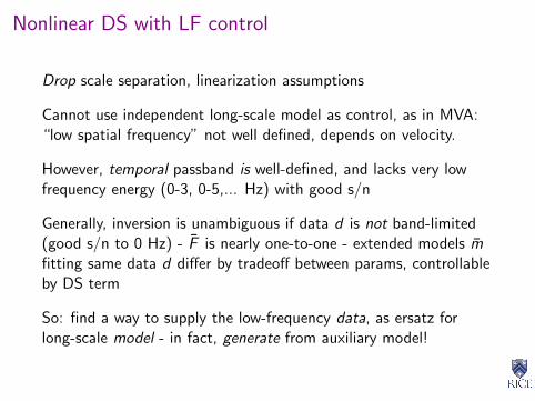
Nonlinear DS with LF control
Drop scale separation, linearization assumptions
Cannot use independent long-scale model as control, as in MVA:“low spatial frequency” not well defined, depends on velocity.
However, temporal passband is well-defined, and lacks very lowfrequency energy (0-3, 0-5,... Hz) with good s/n
Generally, inversion is unambiguous if data d is not band-limited(good s/n to 0 Hz) - F is nearly one-to-one - extended models mfitting same data d differ by tradeoff between params, controllableby DS term
So: find a way to supply the low-frequency data, as ersatz forlong-scale model - in fact, generate from auxiliary model!
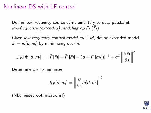
Nonlinear DS with LF control
Define low-frequency source complementary to data passband,low-frequency (extended) modeling op Fl (Fl)
Given low frequency control model ml ∈ M, define extended modelm = m[d ,ml ] by minimizing over m
JDS [m; d ,ml ] = ‖F [m] + Fl [m]− (d + Fl [ml ])]‖2 + σ2
∥∥∥∥∂m
∂s
∥∥∥∥2
Determine ml ⇒ minimize
JLF [d ,ml ] =
∥∥∥∥ ∂∂sm[d ,ml ]
∥∥∥∥2
(NB: nested optimizations!)
Nonlinear DS with LF control
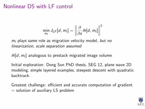
minml
JLF [d ,ml ] =
∥∥∥∥ ∂∂sm[d ,ml ]
∥∥∥∥2
ml plays same role as migration velocity model, but nolinearization, scale separation assumed
m[d ,ml ] analogous to prestack migrated image volume
Initial exploration: Dong Sun PhD thesis, SEG 12, plane wave 2Dmodeling, simple layered examples, steepest descent with quadraticbacktrack.
Greatest challenge: efficient and accurate computation of gradient= solution of auxiliary LS problem
Example: DS Inversion with LF control, free surface
0
0.2
0.4
z (k
m)
0 2x (km)
0.6 0.8 1.0 1.2x10⁴
MPa
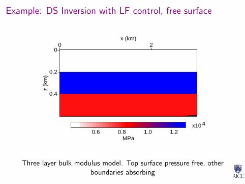
Three layer bulk modulus model. Top surface pressure free, otherboundaries absorbing
Example: DS Inversion with LF control, free surface
0
0.5
1.0time
(s)
-0.09 -0.08 -0.06 -0.04 -0.02 0.00 0.02 0.04 0.06 0.08sign(p)*p^2 (s^2/km^2)
-1000 -500 0 500 1000
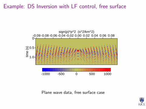
Plane wave data, free surface case
Example: DS Inversion with LF control, free surface
0
0.1
0.2
0.3
0.4
0.5
z (k
m)
-0.08 -0.06 -0.04 -0.02 0 0.02 0.04 0.06 0.08sign(p)*p^2 (s^2/km^2)
-500 0 500MPa
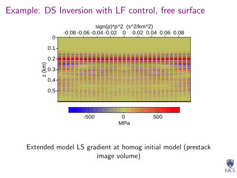
Extended model LS gradient at homog initial model (prestackimage volume)
Example: DS Inversion with LF control, free surface
0
0.1
0.2
0.3
0.4
0.5
z (k
m)
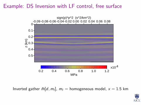
-0.09-0.08-0.06-0.04-0.02 0.00 0.02 0.04 0.06 0.08sign(p)*p^2 (s^2/km^2)
0.2 0.4 0.6 0.8 1.0 1.2x10⁴
MPa
Inverted gather m[d ,ml ], ml = homogeneous model, x = 1.5 km
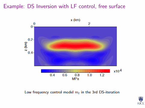
Example: DS Inversion with LF control, free surface
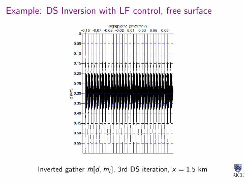
Example: DS Inversion with LF control, free surface
Inverted gather m[d ,ml ], 3rd DS iteration, x = 1.5 km
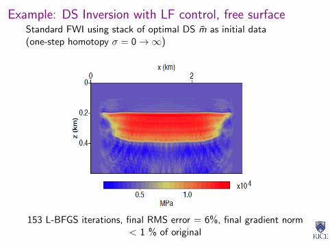
Example: DS Inversion with LF control, free surfaceStandard FWI using stack of optimal DS m as initial data(one-step homotopy σ = 0→∞)
153 L-BFGS iterations, final RMS error = 6%, final gradient norm< 1 % of original
Space Shift DS
Defect in version 1 of DS already known in MVA context:
Image gathers generated from individual surface databins may not be flat, even when migration velocity isoptimally chosen (Nolan & S, 97, Stolk & S 04)
Source of kinematic artifacts obstructing flatness: multiple raypaths connecting sources, receivers with reflection points.
Therefore version 1 of DS only suitable for mild lateralheterogeneity. Must use something else to identify complexrefracting structures
Space Shift DS
For MVA, remedy is known: use space-shift image gathers δm (deHoop, Stolk & S 09)
Claerbout’s imaging principle (71): velocity is correct if energy inδm(x,h) is focused at h = 0 (h = subsurface offset)
Quantitative measure of focus: choose P(h) so that P(0) = 0,P(h) > 0 if h 6= 0, minimize∑
x,h
|P(h)δm[m0](x,h)|2
(e. g. P(h) = |h|).
MVA based on this principle by Shen, Stolk, & S. 03, Shen et al.05, Albertin 06, 11, Kubir et al. 07, Fei & Williamson 09, 10, Tang& Biondi 11, others - survey in Shen & S 08. Gradient issues: Fei& Williamson 09, Vyas 09.
Space Shift DS
Extension to nonlinear problems - how is δm[x,h] the output of anadjoint derivative?
Answer: Replace coefficients m in wave equation with operators m:e. g. κ[u](x) =
∫dhκ(x,h)u(x + h). Physical case: multiplication
operators κ(x,h) = κ(x)δ(h). Then
δm[m0] = DF [m0]T (d − F [m])
for resulting extended fwd map F
⇒ Version 2 of nonlinear DS. Physical case =no-action-at-a-distance principle of continuum mechanics =nonlinear version of Claerbout’s imaging principle (S, 08).Mathematical foundation: Blazek, Stolk & S. 08.

Agenda
Overview
Challenges for FWI
Extended modeling
Summary
Summary
I restriction to low frequency data makes FWI objective morequadratic, just like you always thought
I transmission inversion is easier than reflection for linearreasons, so MVA seems like a good place to look for reflectioninversion approaches
I extended modeling provides a formalism for expressing MVAobjectives that extend naturally to nonlinear FWI, viacontinuation - provision of starting models, route to FWIsolution
I positive early experience with “gather flattening” nonlineardifferential semblance
I “survey sinking” NDS involves wave equations with operatorcoefficients
I Patrick’s fingerprints are all over this subject

Thanks to...
I Florence Delprat and other organizers, EAGE
I my students and postdocs, particularly Dong Sun, Peng Shen,Chris Stolk, Kirk Blazek, Joakim Blanch, Cliff Nolan, SueMinkoff, Mark Gockenbach, Roelof Versteeg, Michel Kern
I National Science Foundation
I Sponsors of The Rice Inversion Project
I Patrick Lailly, for inspired, inspiring, and fundamentalcontributions to this field