object tracking using kalman and particle filtering …...object tracking using kalman and particle...

Object Tracking using Kalman and Particle filtering Techniques

Department of Electronics and Communication Engineering

National Institute of Technology Rourkela

Rourkela, Odisha, 769008, India

2015

Object Tracking using Kalman and Particle filtering Techniques

A thesis submitted in partial fulfillment of the requirement for the degree of

Master of Technology

In Electronics and Communication Engineering Specialization: Signal and Image Processing

By

Kodali Sai Krishna Roll No. 213EC6261

Under the Supervision of Dr. A.K.SAHOO

Department of Electronics and Communication Engineering

National Institute of Technology Rourkela

Rourkela, Odisha, 769008, India

2015

DECLARATION

I certify that,

a. The work presented in this thesis is an original content of the research done

by myself under the general supervision of my supervisor.

b. The work has not been submitted to any other institute for any degree or

diploma.

c. The data used in this work is taken from free source and its credit has been

cited in reference.

d. The materials (data, theoretical analysis and text) used for this work has

been given credit by citing them in the text of thesis and their details in the

references.

e. I have followed the thesis guidelines provided by the institution

KODALI SAI KRISHNA

DEPARTMENT OF ELECRTONICS AND COMMUNICATION

NATIONAL INSTITUTE OF TECHNOLOGY,

ROURKELA, ODISHA -769008.

CERTIFICATE

Dr. A.K.SAHOO

This is to certify that the work done in the report entitled “Object Tracking using

Kalman and Particle filtering Techniques” by “KODALI SAI KRISHNA” is a

record of research work carried out by him in National Institute of Technology, Rourkela

under my supervision and guidance during 2014-15 in partial fulfillment of the

requirement for the award of degree in Master of Technology in Electronics and

Communication Engineering (Signal and Image Processing), National Institute of

Technology, Rourkela. To the best of my knowledge, this thesis has not been submitted

for any degree or diploma.

DEPARTMENT OF ELECRTONICS AND COMMUNICATION

NATIONAL INSTITUTE OF TECHNOLOGY,

ROURKELA, ODISHA -769008.

Date

ACKNOWLEDGEMENT This research work is one of the significant achievements in my life and is made possible because

of the unending encouragement and motivation given by so many in every part of my life. It is

immense pleasure to have this opportunity to express my gratitude and regards to them.

Firstly, I would like to express my gratitude and sincere thanks to Dr. A.K.SAHOO, my

supervisor, Department of Electronics and Communication Engineering for his esteemed

supervision and guidance during the tenure of my project work. His valuable advices have

motivated me a lot when I feel saturated in my work. His impartial feedback in every walk of the

research has made me to approach a right way in excelling the work. It would also like to thank

him for providing best facilities in the department.

I am very much indebted to Prof. S. K. Patra and Prof. K. K. Mohapatra for teaching me subjects

that proved to be very helpful in my work. My special thanks go to Prof. S. Meher, Prof. L.P. Roy

and Prof. S. Ari for contributing towards enhancing the quality of the work and eventually shaping

my thesis.

Lastly, I would like to express my love and heartfelt respect to my parents, sister and brothers

for their consistent support, encouragement in every walk of my life without whom I would be

nothing.

Kodali Sai Krishna

I

ABSTRACT

Object tracking has been an active field of research in the past decade. There are many challenges

in tracking the object understand in which kind of system model it is moving and which type of

noise it is taking . System model can be either linear or nonlinear or coordinated turn model and

such noise can be either Gaussian or non-Gaussian depending on the type of filter chosen,

Extended Kalman filter (EKF) is widely used for tracking moving objects like missiles, aircrafts

and robots. Here analyse the instance of a single sensor or observer bearing only tracking (BOT)

problem for two different models. In model 1, the target is assumed to have a constant velocity

and constant course. In model 2, the target is assumed to follow a coordinated turn model with

constant velocity but varying course. Extended Kalman Filter is used to track the target in both

cases.

For some application part, it is getting to be necessary to include components of nonlinearity

and non-Gaussianity with a specific end goal to model exactly the essential dynamics of a system.

The nonlinear extended Kalman filter (EKF) and the particle filter (PF) algorithms are used and

compared the manoeuvring object tracking with bearing-only measurements. We also propose a

proficient system for resampling particles to decrease the impact of degeneracy effect of particle

propagation in the particle filter (PF) algorithm. One of the particle filter (PF) technique is

sequential importance resampling (SIR). It is discussed and compared with the standard EKF

through an illustrative example.

Keywords: Bearing Only Tracking (BOT), Extended Kalman filter (EKF), Particle Filter (PF),

Sequential Importance Resampling (SIR).

II

Table of Contents ABSTRACT ...................................................................................................................................................... ii

List of Figures ............................................................................................................................................. v

List of acronyms.................................................................................................................................... vi

CHAPTER1 ..................................................................................................................................................... 1

Chapter1 ....................................................................................................................................................... 2

Introduction .................................................................................................................................................. 2

1.1 Tracking: ............................................................................................................................................. 2

1.2 Filter.................................................................................................................................................... 2

1.2.1 Adaptive Filter ............................................................................................................................. 2

1.3 Different system models .................................................................................................................... 4

1.4 Motivation: ......................................................................................................................................... 5

1.5 Problem Statement ............................................................................................................................ 6

1.6 Organization of Thesis: ....................................................................................................................... 6

Chapter 2 ...................................................................................................................................................... 9

KALMAN FILTER ............................................................................................................................................ 9

2.1 Introduction: ....................................................................................................................................... 9

2.2 Linear recursive estimator .................................................................................................................. 9

2.3 Basic Kalman filter model ................................................................................................................. 10

2.3.1 Prediction: ................................................................................................................................. 11

2.3.2 Update: ...................................................................................................................................... 11

Chapter3 ..................................................................................................................................................... 14

EXTENDED KALMAN FILTER ........................................................................................................................ 14

3.1 Introduction ...................................................................................................................................... 14

3.2 Extended kalman filter ..................................................................................................................... 16

3.2.1 Ekf algorithm ............................................................................................................................. 16

Prediction: .......................................................................................................................................... 17

Kalman gain: ....................................................................................................................................... 17

Update ................................................................................................................................................ 17

3.3 EKF WITH SINGLE SENSOR CASE ....................................................................................................... 18

3.4 EKF WITH MULTI SENSOR CASE ........................................................................................................ 19

3.4.1 First order Ekf ............................................................................................................................ 20

3.4.1 Second order Ekf ....................................................................................................................... 20

3.5 ILLUSTRATION ................................................................................................................................... 21

3.5.1 Illustration with different models ............................................................................................. 23

III

3.6 Disadvantages of extended kalman filter: ........................................................................................ 27

Chapter4 ..................................................................................................................................................... 29

PARTICLE FILTER ......................................................................................................................................... 29

4.1 Introduction ...................................................................................................................................... 29

4.2 Sequential importance sampling ...................................................................................................... 30

4.3 Basic Particle filter model ................................................................................................................. 31

4.4 Basic algorithm steps ........................................................................................................................ 31

4.5 Sample impoverishment: ................................................................................................................. 34

4.5.1 Regularized particle filter: ......................................................................................................... 34

4.3 Comparison to the discrete Kalman filter ........................................................................................ 35

Chapter5 ..................................................................................................................................................... 37

EXPERIMENTAL RESULTS AND DISCUSSION ............................................................................................... 37

Constant Velocity and Course Target ................................................................................................. 37

Constant Velocity and Varying Course Target .................................................................................... 38

Chapter6 ................................................................................................................................................. 43

Conclusion and Future Work .................................................................................................................. 43

REFERENCES ........................................................................................................................................... 44

IV

List of Figures

Fig 1.1 General Adaptive Model 3

Fig 1.2 Adaptive filter 3

Fig 4.1.Comparison between kalman and particle filters 35

Fig 5.1 tracking with kalman filter case1 37

Fig 5.2 tracking with kalman filter case2 37

Fig 5.3 tracking the object path for a manoeuvuring targert case1 38

Fig5.4 tracking the object path for a manoeuvuring targert case1 38

Fig 5.5tracking one dimensional nonlinear example of particle filter 39

Fig 5.6 tracking two imensional nonlinear example of particle filter 40

Fig 5.7tracking comparision between particle filter and extende kalman filters 41

V

List of acronyms

BOT Bearing Only Tracking

EKF Extended Kalman Filter

PF Particle Filter

SIR Sequential Importance Resampling

IMM Inter active Multiple Model

GHKF Gauss-Hermite Kalman Filter

SIS Sequential Importance Sampling

𝑁𝑁𝑒𝑒𝑒𝑒𝑒𝑒 Effective Sample Size

VI

CHAPTER1

INTRODUCTION

1

Chapter1

Introduction

1.1 Tracking: Tracking means finding the position of object with respect to time, in general while tracking the

object first step is detection of the object, next tracking the object and finally observing its

behaviour with respect to time. Object tracking is required in various tasks in real life, such as

surveillance, video compression and video analysis. While tracking the object trajectory there exist

certain problems those will be solved by different tracking techniques.

1.2 Filter The term filter means it accepts certain type of data as input and processes it, transformed and

then outputs the transformed data. The term filter comes in tracking the object trajectory is due to

while tracking the object path there exists certain uncertainties comes into picture those are noise,

occlusions, appearance changes. One of the technique to remove the existed noise is filtering. The

term filtering fundamentally implies the methodology of separating out the noises in estimations

and giving an ideal assessment to the state. Filter in generally removes those existed noises. Here

filtering term is used while tracking the object so that it is called tracking with filters.

1.2.1 Adaptive Filter The term Adaptive represents iterative in nature, in general adaptive filter means it models

computation between two devices in iterative manner. In adaptive algorithm it portrays how the

parameters are adjusted from one time moment to next time moment. In general in adaptive filter

it takes input signal samples x(n) and process it and gives the output signal samples let us consider

these output samples as y(n) in adaptive filter these output samples are varied from one time

moment to next time moment by adjusting and taking certain

2

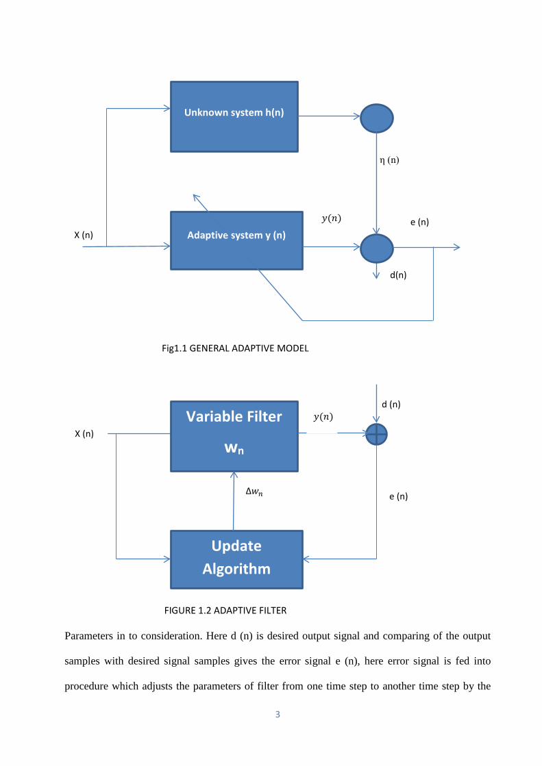
Fig1.1 GENERAL ADAPTIVE MODEL

FIGURE 1.2 ADAPTIVE FILTER

Parameters in to consideration. Here d (n) is desired output signal and comparing of the output

samples with desired signal samples gives the error signal e (n), here error signal is fed into

procedure which adjusts the parameters of filter from one time step to another time step by the

Variable Filter

wn

Update Algorithm

X (n)

𝑦𝑦(𝑛𝑛)

Δ𝑤𝑤𝑛𝑛

e (n)

Unknown system h(n)

Adaptive system y (n) X (n)

𝑦𝑦(𝑛𝑛)

η (n)

d (n)

e (n)

d(n)

3

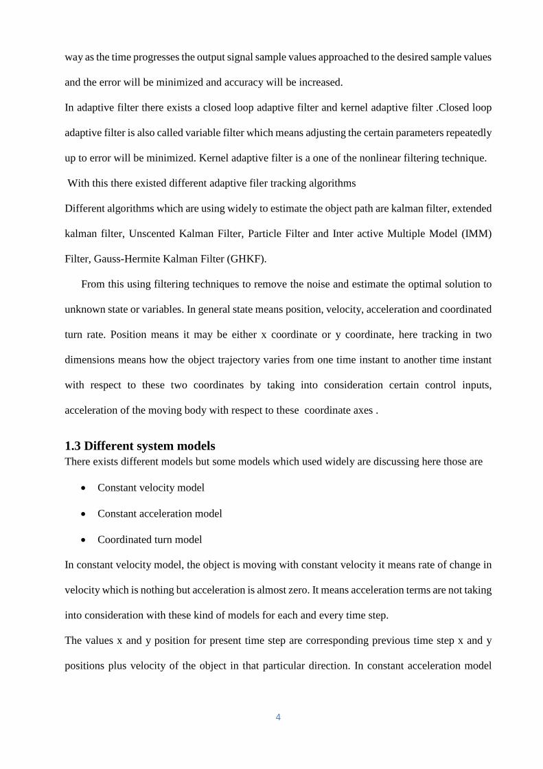
way as the time progresses the output signal sample values approached to the desired sample values

and the error will be minimized and accuracy will be increased.

In adaptive filter there exists a closed loop adaptive filter and kernel adaptive filter .Closed loop

adaptive filter is also called variable filter which means adjusting the certain parameters repeatedly

up to error will be minimized. Kernel adaptive filter is a one of the nonlinear filtering technique.

With this there existed different adaptive filer tracking algorithms

Different algorithms which are using widely to estimate the object path are kalman filter, extended

kalman filter, Unscented Kalman Filter, Particle Filter and Inter active Multiple Model (IMM)

Filter, Gauss-Hermite Kalman Filter (GHKF).

From this using filtering techniques to remove the noise and estimate the optimal solution to

unknown state or variables. In general state means position, velocity, acceleration and coordinated

turn rate. Position means it may be either x coordinate or y coordinate, here tracking in two

dimensions means how the object trajectory varies from one time instant to another time instant

with respect to these two coordinates by taking into consideration certain control inputs,

acceleration of the moving body with respect to these coordinate axes .

1.3 Different system models There exists different models but some models which used widely are discussing here those are

• Constant velocity model

• Constant acceleration model

• Coordinated turn model

In constant velocity model, the object is moving with constant velocity it means rate of change in

velocity which is nothing but acceleration is almost zero. It means acceleration terms are not taking

into consideration with these kind of models for each and every time step.

The values x and y position for present time step are corresponding previous time step x and y

positions plus velocity of the object in that particular direction. In constant acceleration model

4

object is moving with constant acceleration here constant acceleration term is included for each

and every time instant while updating the positions of x and y coordinates.

In coordinated turn model it includes one more new term that is coordinated turn rate which is also

called as angular turn rate measured in radians per second here in this model, it takes velocity term

but it can’t take the acceleration term while updating the x and y coordinates, it takes the newly

included term coordinated turn rate which is denoted by w in general, this term also has been

included while updating the x and y coordinates.

In constant velocity model for present x or y position it wants previous x or y position and its

corresponding x or y position velocity it means it is looking like a linear model so constant velocity

model is also called linear model.

In constant acceleration model while measuring present x or y positions it wants previous x or y

positions and corresponding velocities and corresponding acceleration terms are included. Here

because of only one term this model seems to be not a linear model that term is acceleration term

but any way this is not that much of nonlinear in nature. In coordinated turn model with that

constant velocity term for each and every coordinate updating coordinated turn rate also has been

included because of this term this model is seems to be nonlinear model.

1.4 Motivation: The main theme of object tracking is based on the tracking the object path in the unknown

environment. Tracking the object path within its environment is a crucial task and has been

extensively explored in many research papers. Tracking the object with different nonlinear models

has been studied in many other papers. There is need for highly accurate or optimal filtering

techniques to track the object path. While tracking the object path it will be affected by different

obstacles those are occlusions, noises and scene changes. These noise terms will be removed by

using different adaptive filtering techniques. Hence to address these problems a robust and

simple,yet efficient object tracking technique is necessary. The typical models discussed below as

described in gives us an idea of the various steps involved in tracking the object trajectory process.

5

1.5 Problem Statement In light of all the obstacles plaguing the object tracking process a need for an accurate and

estimation system is required. Hence the problem at hand is to track the object trajectory as the

object moves along the unknown environment. To track the object trajectory bearing

measurements is also essential. Adaptive filter algorithms estimate the unknown position but there

existed a lot of disturbances while estimating the states of the object. An advanced algorithm

estimation approach is to be taken in which gradually update the particle positions with respect to

its initial location and update the particle weights with respect to system dynamics.

1.6 Organization of Thesis: This thesis consists of a total of six chapters organized as below

Chapter 1. This chapter gives a brief introduction to the object tacking that is detecting

tracking the object trajectory which is varying with respect to time, and the different system

models in which object is moving and then little bit discussion about the filtering, and

adaptive filtering algorithms.

Chapter 2. This chapter will give description to the kalman filter, how the kalman filter

works, and the models for which it works well and how it tracks the object trajectory in

unknown environment and the steps which this kalman filter algorithm takes to give best

solution for object path tracking.

Chapter 3. This chapter will give detailed description to the extended kalman filter, how it

over comes the disadvantages in kalman filter and for the models which it gives best

estimation, and how the jacobian and hessian matrices approximates the nonlinearity and

the algorithm steps which it takes to track the nonlinear object path effectively.

Chapter 4. This chapter will discuss the complete description to the particle filter, here we

also discussed the disadvantages existed in extended kalman filter, how these will be solved

6

in particle filter, compared it with discrete kalman filter and the basic steps to implement

the particle filter algorithm.

Chapter 5. The results of the trajectory paths obtained by applying the different filtering

techniques to different system models are presented in this chapter. Evaluation and analysis

of these results is also presented in this chapter.

Chapter 6. This chapter will discuss Conclusion and also future improvements

7

CHAPTER2 KALMAN FILTER

8

Chapter 2

KALMAN FILTER

2.1 Introduction: The Kalman filter was at first introduced by Rudolph E. Kalman in his innovative Paper

(Kalman, 1960). Kalman filter is also called as linear quadratic estimator, it estimates the unknown

variables by taking series of measurements which contains noise and other inaccuracies and

estimates the unknown variables. Kalman filter is also called as linear state space estimator which

uses linear state and measurement equations. Kalman filter operates recursively on stream of noisy

input data to find the optimal estimate of unknown state.

2.2 Linear recursive estimator Kalman filter operates by taking linear models and noise is Gaussian noise then it gives better

results by minimizing the mean square error. One most praised apparatuses in straight minimum

mean-squares estimation hypothesis, to be specific the Kalman channel. The channel has a

personal connection with versatile channel hypothesis, to such an extent that a strong

comprehension of its usefulness can recommend expansions of traditional versatile plans. After

we have advanced adequately enough in our treatment of versatile channels. At that stage, we

might tie up the Kalman channel with versatile slightest squares hypothesis and show how it can

rouse helpful augmentations.

Kalman filter is a recursive estimator it means that while estimating the current state it

requires previous state and its current measurements. These two are sufficient to estimate the

current state.

Kalman filter averages the prediction of system state with new measurement by using

weighted average phenomenon. The reason behind the weighted average is to estimate the state

with lesser uncertainty that is for more accurate estimated values. The estimated value through

weighted average lies between predicted and measurement values. With the new gauge and its

9

covariance advising the expectation utilized as a part of the taking after cycle. The Kalman channel

is a proficient strategy for deciding the advancements, when the perception process emerges from

a limited dimensional direct state-space model, Kalman filter uses system model and control inputs

to that corresponding model and it takes multiple series measurements in to consideration to

estimate the unknown variables, which are varying continuously with time. This gives better

estimate compared to the single measurement alone.

Kalman filter gives a recursive solution to discrete data linear filtering issues. Kalman filter is the

subject of broad examination and application, especially in the zone of self-sufficient or aided

route. It can estimate the state of the system very accurately when the system is unknown also and

so it is very powerful linear recursive estimator of unknown state. Kalman filter is basically an

ideal recursive information handling algorithm that mixes all accessible data measurement outputs

and it has the knowledge about the system model, measurement sensors and then it can estimate

the state of unknown variables by the way mean square error will be minimized.

Kalman filter is one of simplest linear state space model used widely in present days if

the known system and measurement models are linear. While estimating the unknown state

variables recursively with time there is certain uncertainty in measurement values. Uncertainty is

that process noise and measurement noise included in the measured values and that noise included

must be Gaussian in nature while kalman filter is using to estimate the unknown state variables.

From this we can’t model the system entirely deterministically. Kalman filter uses linear equation

systems with white Gaussian noises as standard model.

2.3 Basic Kalman filter model Kalman filter uses two steps while estimating the unknown states.

• Prediction step

• Updating step

10

2.3.1 Prediction: Forecast type of the Kalman channel depends on propagation of the one-stage expectation. One

more implementation of kalman filter also known as time and measurement update form. In

Prediction step current time state estimate is measured from previous time step. This estimate is

also known as a priori state estimate.it does not require any measurement (observation) values.

Prediction step equations are written as

Here prediction measurements are time update equations that above two equations are a priori

state estimate and a priori error covariance estimates respectively.

2.3.2 Update: In update step, by taking measurement (observation) value in to consideration updating the

apriori state estimate to improve accuracy of estimated state. The estimate after including

observation value is called a posterior state estimate.

Update step equations are written as

( ) ( ) ( )1|^

−−= ttytyte (2.3)

( ) )()()1|().( '~

tRtCttptCtR vvee +−= (2.4)

( ) ( )tRtCttptK ee1'

~)()1|( −−= (2.5)

( ) ( ) ( ) ( )tetKttxttx .1||^^

+−= (2.6)

( ) ( )[ ] )1|()|(~~

−−= ttptCtKIttp (2.7)

Here )1|(^

−ttx and )1|(~

−ttp are predicted state and covariance of the state without knowing the

value of measurement value.

)1()1()1()1|1().1()1|(^^

−+−−+−−−=− tRtutBttxtAttx vv

)1()1()1|1().1()1|( '~~

−+−−−−=− tRtAttptAttp ww

(2.2)

(2.1)

11

Whereas ( )ttx |^

)|(~

ttp are the estimated state and covariance values after knowing the measurement

value.

( )tk Is the Kalman gain at time step t.

( )te Is the residual measurement error on time step t.

( )tRee Is prediction covariance by including measurement value at time step t.

From the above equations predicted, estimated state and covariance matrices, are independent of

measurement values at any time. A, B, C and R known matrices at each and every time interval. It

is known and understood that the Kalman filter has been generally utilized for parameter

estimation in a state-space model. Since it is the ideally recursive linear filter in the Gaussian noise

distribution environment.

12

CHAPTER3 EXTENDED KALMAN FILTER

13

Chapter3

EXTENDED KALMAN FILTER

3.1 Introduction The extended Kalman filter stretches out the scope of Kalman filter to nonlinear ideal separating

problems by shaping a Gaussian rough guess to the joint circulation of state x and estimations y

utilizing a Taylor arrangement based transformation. Here First and second order extended kalman

filters are introduced. To examine and make induction about an element state no less than two

models are obliged first, a model portraying the advancement of the state with time what's more,

second, a model relating the noisy estimations to the state (the estimation model). We will accept

that these models are accessible in a probabilistic structure. The probabilistic state-space plan and

the prerequisite for the upgrading of data on receipt of new estimations are in a perfect world suited

for the Bayesian approach. This gives a thorough general system for element state estimation

issues.

The Bayesian way to deal with element state estimation, one endeavours to build the back

probability likelihood of the state based on all accessible data, including the arrangement of

observed estimations. Since this work encapsulates all available measurable data, it might be said

to be the complete solution to the estimation issue. On a fundamental level evaluation of the state

may be obtained from the probability distribution function. A measure of the exactness of the

estimate may likewise be acquired. For some issues, an assessment is required every time that

estimation is obtained. For this situation, a recursive filter is an advantageous solution. A recursive

sifting approach means that got information can be prepared sequentially rather than as a cluster,

so it is not important to store the complete data set or to reprocess existing information if another

measurement becomes available. Such a channel comprises of essentially two stages: forecast and

upgrade. The forecast stage utilizes the system model to anticipate the state pdf forward starting

14

with one measurement time then onto the next. Since the state is typically subject to unknown

noise. Prediction generally interprets, twists, and spreads the state pdf. The update operation

utilizes the most recent estimation to alter the prediction pdf. This is accomplished utilizing Bayes

hypothesis, which is the mechanism for overhauling learning about the target state in the additional

data from new information.

In many cases dynamic systems are not linear by nature, so the conventional kalman filter can’t

be used in evaluating the condition of such a system. In these kind of systems either measurement

model or motion are nonlinear or any one of these motion or measurement model may be non-

linear. So we portray some augmentations to the kalman filter those are extended kalman filter,

unscented kalman filter, particle filter, gauss newton filter and Interactive Multi Model (IMM)

filter. Out of these extended kalman filter can be evaluate the nonlinear dynamic systems by

shaping Gaussian estimates to the joint distribution of the state x and estimation y. To start with

the Extended Kalman filter (EKF), which is taking into account Taylor series arrangement estimate

of the joint distribution, and after that the Unscented Kalman filter is take in to consideration in

this unscented kalman filter, it takes sigma points into consideration while estimating the unknown

variables. The extended Kalman filter broadens the extent of Kalman channel to nonlinear ideal

separating issues by shaping a Gaussian estimate to the joint distribution of state x and estimations

y utilizing a Taylor arrangement based change. If the non-linearity is up to certain extent extended

kalman filter works fine. If the non-linearity is more and more and joint distribution for the state

and measurement models is non Gaussian it can’t work well or it can’t track the object path

correctly. It means that extended kalman filter is not the best estimate if the joint probability

distribution for those state and measurement models is non Gaussian and system dynamics with

more and more linearity, so we proceeded to one more filter to optimizing the filtering estimate

that is to increase the accuracy and to get best estimation of object trajectory. One filter which

satisfies above criteria very well and gives optimal solution to object path tracking is particle filter.

Particle filter is one of the best solutions of object tracking in signal domain if the system dynamics

15

that may be either system model or measurement models, are nonlinear or joint probability

distribution for these two models is non Gaussian then gives results very accurately that is it tracks

the object trajectory very well. One example of such nonlinearity case is bearing only object

tracking it used is widely in lot of fields. In this there exists certain kind of target which contains

more nonlinearity is maneuvering target means that it has abrupt change in its state by sudden

using of acceleration parameter

3.2 Extended kalman filter The filtering model used in the extended kalman filter is

𝑋𝑋𝑘𝑘+1 = 𝑓𝑓(𝑋𝑋𝑘𝑘,𝑘𝑘) + 𝑤𝑤𝑘𝑘 (3.1)

𝑧𝑧𝑘𝑘 = ℎ(𝑋𝑋𝑘𝑘,𝑘𝑘) + 𝑣𝑣𝑘𝑘 (3.2)

Here 𝑋𝑋𝑘𝑘denotes the state vector at kth time step

𝑤𝑤𝑘𝑘 is the process noise vector

𝑣𝑣𝑘𝑘 is measurement noise vector

𝑓𝑓(𝑋𝑋𝑘𝑘,𝑘𝑘) is nonlinear system state transition function which transits state from one time instant to

another time instant

ℎ(𝑋𝑋𝑘𝑘,𝑘𝑘) is measurement function

𝑧𝑧𝑘𝑘 is measurement state vector at kth time instant

3.2.1 Ekf algorithm Similar to kalman filter extended kalman filter also has two steps to estimate the unknown state or

variables. Those two steps are

• Prediction

• Updating

In prediction step prediction of new state vector and its corresponding covariance will be

calculated for certain time interval by using its dynamic system and measurement models

respectively. After prediction residual measurement error and residual error covariance matrices

16

are calculated and these terms will be used in state and covariance updating, and to evaluate the

kalman gain.

After predicting the state vector and covariance matrices, then next step is updating these state

vector and covariance matrices, then calculating the kalman gain matrix and after getting this

kalman gain final estimation of state vector and covariance matrices will be done by using this

kalman gain term[8],[12].

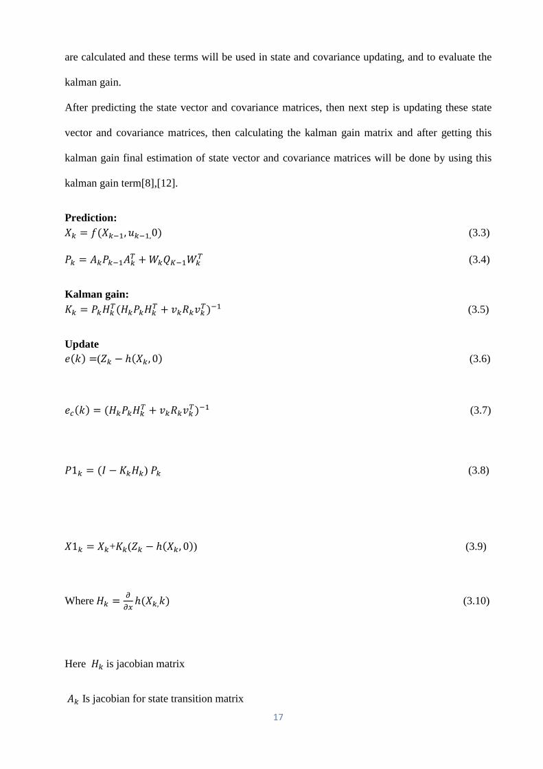
Prediction: 𝑋𝑋𝑘𝑘 = 𝑓𝑓(𝑋𝑋𝑘𝑘−1,𝑢𝑢𝑘𝑘−1,0) (3.3)

𝑃𝑃𝑘𝑘 = 𝐴𝐴𝑘𝑘𝑃𝑃𝑘𝑘−1𝐴𝐴𝑘𝑘𝑇𝑇 + 𝑊𝑊𝑘𝑘𝑄𝑄𝐾𝐾−1𝑊𝑊𝑘𝑘𝑇𝑇 (3.4)

Kalman gain: 𝐾𝐾𝑘𝑘 = 𝑃𝑃𝑘𝑘𝐻𝐻𝑘𝑘𝑇𝑇(𝐻𝐻𝑘𝑘𝑃𝑃𝑘𝑘𝐻𝐻𝑘𝑘𝑇𝑇 + 𝑣𝑣𝑘𝑘𝑅𝑅𝑘𝑘𝑣𝑣𝑘𝑘𝑇𝑇)−1 (3.5)

Update 𝑒𝑒(𝑘𝑘) =(𝑍𝑍𝑘𝑘 − ℎ(𝑋𝑋𝑘𝑘, 0) (3.6)

𝑒𝑒𝑐𝑐(𝑘𝑘) = (𝐻𝐻𝑘𝑘𝑃𝑃𝑘𝑘𝐻𝐻𝑘𝑘𝑇𝑇 + 𝑣𝑣𝑘𝑘𝑅𝑅𝑘𝑘𝑣𝑣𝑘𝑘𝑇𝑇)−1 (3.7)

𝑃𝑃1𝑘𝑘 = (𝐼𝐼 − 𝐾𝐾𝑘𝑘𝐻𝐻𝑘𝑘) 𝑃𝑃𝑘𝑘 (3.8)

𝑋𝑋1𝑘𝑘 = 𝑋𝑋𝑘𝑘+𝐾𝐾𝑘𝑘(𝑍𝑍𝑘𝑘 − ℎ(𝑋𝑋𝑘𝑘, 0)) (3.9)

Where 𝐻𝐻𝑘𝑘 = 𝜕𝜕𝜕𝜕𝜕𝜕ℎ(𝑋𝑋𝑘𝑘,𝑘𝑘) (3.10)

Here 𝐻𝐻𝑘𝑘 is jacobian matrix

𝐴𝐴𝑘𝑘 Is jacobian for state transition matrix

17

𝑒𝑒(𝑘𝑘) is measurement error vector

𝑒𝑒𝑐𝑐(𝑘𝑘) is measurement error covariance

𝑄𝑄𝐾𝐾−1 is process noise covariance matrix

𝑅𝑅𝑘𝑘 is measurement noise covariance matrix

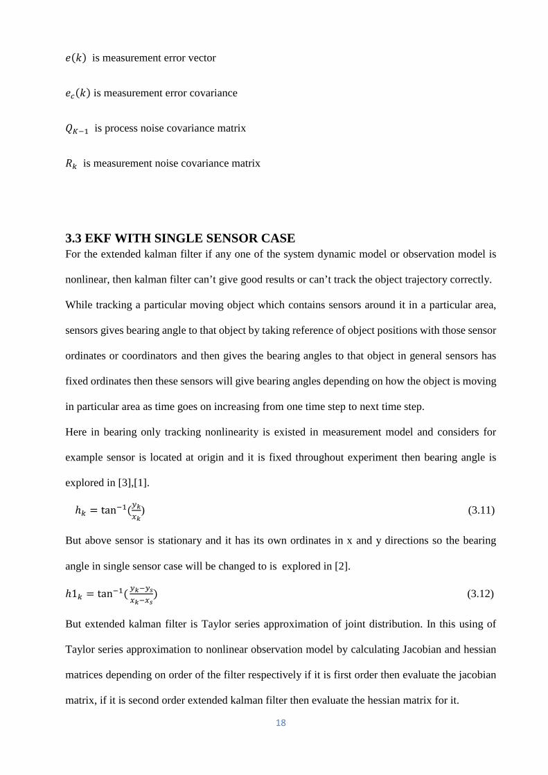
3.3 EKF WITH SINGLE SENSOR CASE For the extended kalman filter if any one of the system dynamic model or observation model is

nonlinear, then kalman filter can’t give good results or can’t track the object trajectory correctly.

While tracking a particular moving object which contains sensors around it in a particular area,

sensors gives bearing angle to that object by taking reference of object positions with those sensor

ordinates or coordinators and then gives the bearing angles to that object in general sensors has

fixed ordinates then these sensors will give bearing angles depending on how the object is moving

in particular area as time goes on increasing from one time step to next time step.

Here in bearing only tracking nonlinearity is existed in measurement model and considers for

example sensor is located at origin and it is fixed throughout experiment then bearing angle is

explored in [3],[1].

ℎ𝑘𝑘 = tan−1(𝑦𝑦𝑘𝑘𝜕𝜕𝑘𝑘

) (3.11)

But above sensor is stationary and it has its own ordinates in x and y directions so the bearing

angle in single sensor case will be changed to is explored in [2].

ℎ1𝑘𝑘 = tan−1( 𝑦𝑦𝑘𝑘−𝑦𝑦𝑠𝑠𝜕𝜕𝑘𝑘−𝜕𝜕𝑠𝑠

) (3.12)

But extended kalman filter is Taylor series approximation of joint distribution. In this using of

Taylor series approximation to nonlinear observation model by calculating Jacobian and hessian

matrices depending on order of the filter respectively if it is first order then evaluate the jacobian

matrix, if it is second order extended kalman filter then evaluate the hessian matrix for it.

18

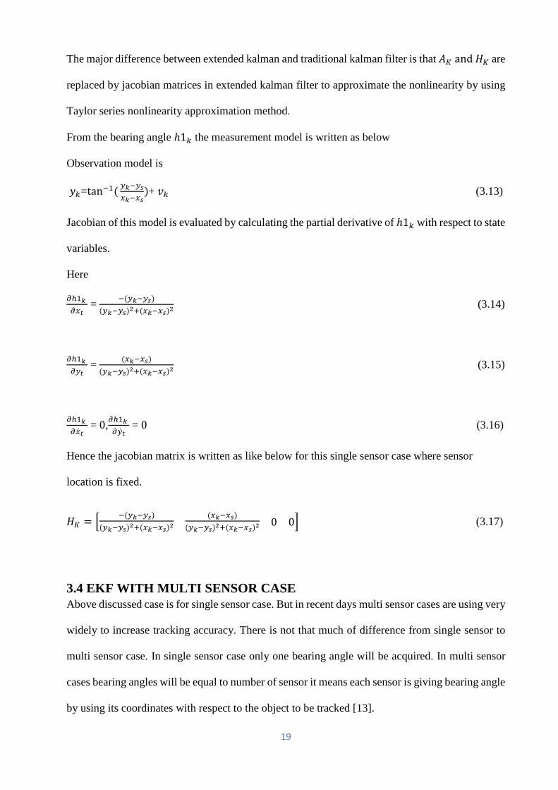
The major difference between extended kalman and traditional kalman filter is that 𝐴𝐴𝐾𝐾 and 𝐻𝐻𝐾𝐾 are

replaced by jacobian matrices in extended kalman filter to approximate the nonlinearity by using

Taylor series nonlinearity approximation method.

From the bearing angle ℎ1𝑘𝑘 the measurement model is written as below

Observation model is

𝑦𝑦𝑘𝑘=tan−1( 𝑦𝑦𝑘𝑘−𝑦𝑦𝑠𝑠𝜕𝜕𝑘𝑘−𝜕𝜕𝑠𝑠

)+ 𝑣𝑣𝑘𝑘 (3.13)

Jacobian of this model is evaluated by calculating the partial derivative of ℎ1𝑘𝑘 with respect to state

variables.

Here

𝜕𝜕ℎ1𝑘𝑘 𝜕𝜕𝜕𝜕𝑡𝑡

= −(𝑦𝑦𝑘𝑘−𝑦𝑦𝑠𝑠)(𝑦𝑦𝑘𝑘−𝑦𝑦𝑠𝑠)2+(𝜕𝜕𝑘𝑘−𝜕𝜕𝑠𝑠)2

(3.14)

𝜕𝜕ℎ1𝑘𝑘 𝜕𝜕𝑦𝑦𝑡𝑡

= (𝜕𝜕𝑘𝑘−𝜕𝜕𝑠𝑠)(𝑦𝑦𝑘𝑘−𝑦𝑦𝑠𝑠)2+(𝜕𝜕𝑘𝑘−𝜕𝜕𝑠𝑠)2

(3.15)

𝜕𝜕ℎ1𝑘𝑘 𝜕𝜕�̇�𝜕𝑡𝑡

= 0,𝜕𝜕ℎ1𝑘𝑘 𝜕𝜕�̇�𝑦𝑡𝑡

= 0 (3.16)

Hence the jacobian matrix is written as like below for this single sensor case where sensor

location is fixed.

𝐻𝐻𝐾𝐾 = � −(𝑦𝑦𝑘𝑘−𝑦𝑦𝑠𝑠)(𝑦𝑦𝑘𝑘−𝑦𝑦𝑠𝑠)2+(𝜕𝜕𝑘𝑘−𝜕𝜕𝑠𝑠)2

(𝜕𝜕𝑘𝑘−𝜕𝜕𝑠𝑠)(𝑦𝑦𝑘𝑘−𝑦𝑦𝑠𝑠)2+(𝜕𝜕𝑘𝑘−𝜕𝜕𝑠𝑠)2 0 0� (3.17)

3.4 EKF WITH MULTI SENSOR CASE Above discussed case is for single sensor case. But in recent days multi sensor cases are using very

widely to increase tracking accuracy. There is not that much of difference from single sensor to

multi sensor case. In single sensor case only one bearing angle will be acquired. In multi sensor

cases bearing angles will be equal to number of sensor it means each sensor is giving bearing angle

by using its coordinates with respect to the object to be tracked [13].

19

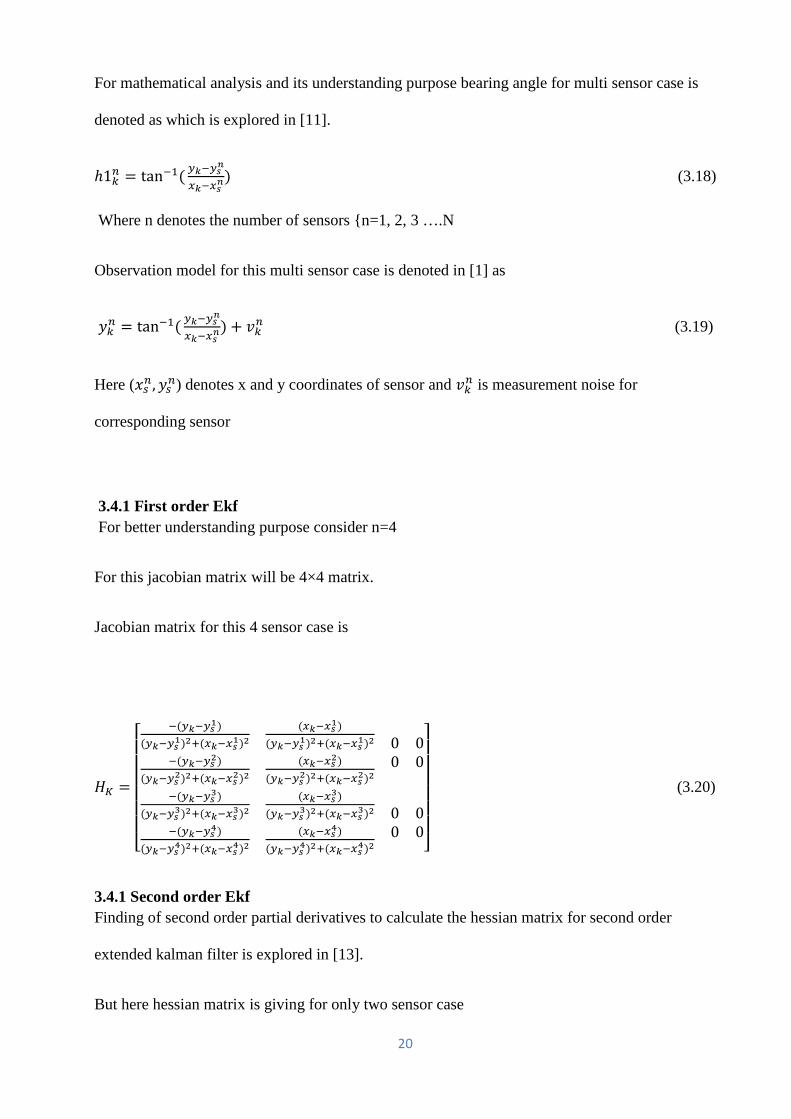
For mathematical analysis and its understanding purpose bearing angle for multi sensor case is

denoted as which is explored in [11].

ℎ1𝑘𝑘𝑛𝑛 = tan−1( 𝑦𝑦𝑘𝑘−𝑦𝑦𝑠𝑠𝑛𝑛

𝜕𝜕𝑘𝑘−𝜕𝜕𝑠𝑠𝑛𝑛) (3.18)

Where n denotes the number of sensors {n=1, 2, 3 ….N

Observation model for this multi sensor case is denoted in [1] as

𝑦𝑦𝑘𝑘𝑛𝑛 = tan−1( 𝑦𝑦𝑘𝑘−𝑦𝑦𝑠𝑠𝑛𝑛

𝜕𝜕𝑘𝑘−𝜕𝜕𝑠𝑠𝑛𝑛) + 𝑣𝑣𝑘𝑘𝑛𝑛 (3.19)

Here (𝑥𝑥𝑠𝑠𝑛𝑛,𝑦𝑦𝑠𝑠𝑛𝑛) denotes x and y coordinates of sensor and 𝑣𝑣𝑘𝑘𝑛𝑛 is measurement noise for

corresponding sensor

3.4.1 First order Ekf For better understanding purpose consider n=4

For this jacobian matrix will be 4×4 matrix.

Jacobian matrix for this 4 sensor case is

𝐻𝐻𝐾𝐾 =

⎣⎢⎢⎢⎢⎢⎢⎡

−(𝑦𝑦𝑘𝑘−𝑦𝑦𝑠𝑠1)(𝑦𝑦𝑘𝑘−𝑦𝑦𝑠𝑠1)2+(𝜕𝜕𝑘𝑘−𝜕𝜕𝑠𝑠1)2

(𝜕𝜕𝑘𝑘−𝜕𝜕𝑠𝑠1)(𝑦𝑦𝑘𝑘−𝑦𝑦𝑠𝑠1)2+(𝜕𝜕𝑘𝑘−𝜕𝜕𝑠𝑠1)2



0 00 0





0 00 0

⎦⎥⎥⎥⎥⎥⎥⎤

(3.20)

3.4.1 Second order Ekf Finding of second order partial derivatives to calculate the hessian matrix for second order

extended kalman filter is explored in [13].

But here hessian matrix is giving for only two sensor case

20

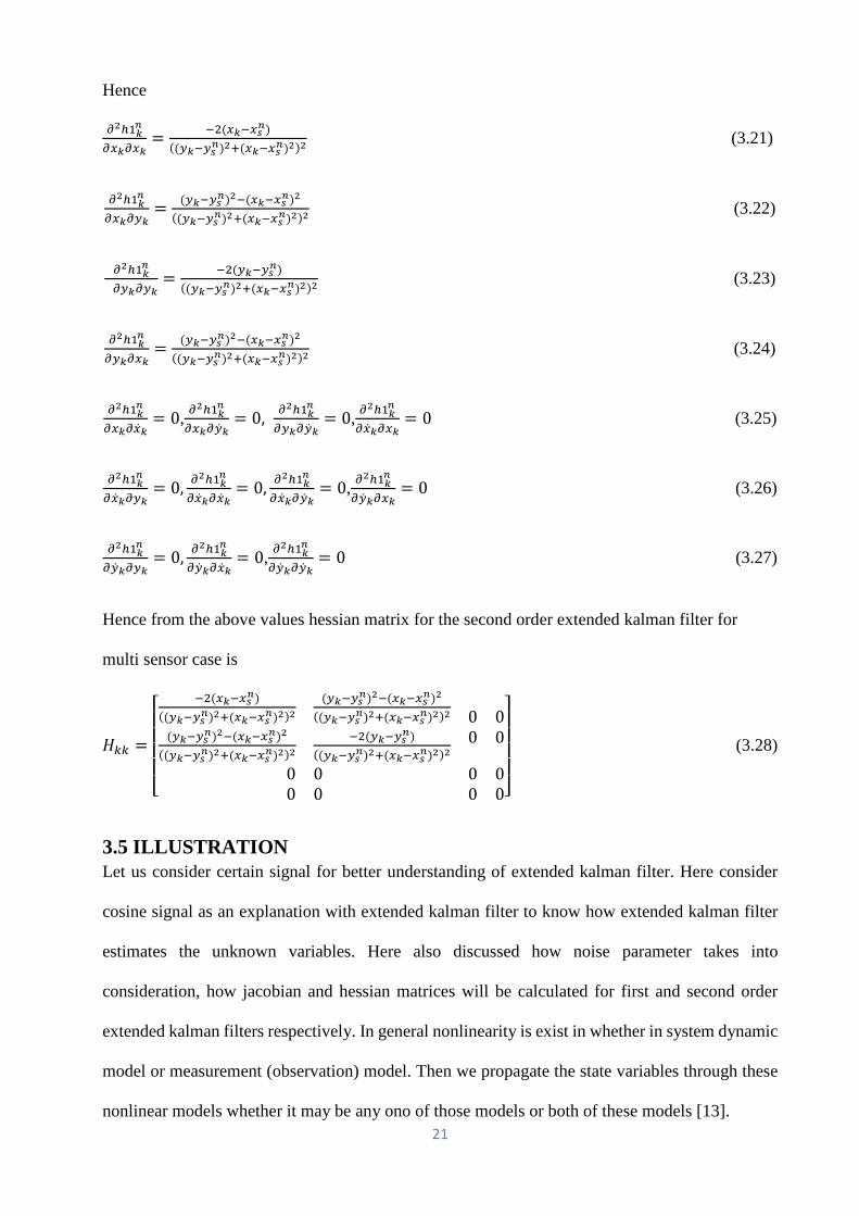
Hence

𝜕𝜕2ℎ1𝑘𝑘𝑛𝑛

𝜕𝜕𝜕𝜕𝑘𝑘𝜕𝜕𝜕𝜕𝑘𝑘= −2(𝜕𝜕𝑘𝑘−𝜕𝜕𝑠𝑠𝑛𝑛)

((𝑦𝑦𝑘𝑘−𝑦𝑦𝑠𝑠𝑛𝑛)2+(𝜕𝜕𝑘𝑘−𝜕𝜕𝑠𝑠𝑛𝑛)2)2 (3.21)


𝜕𝜕𝜕𝜕𝑘𝑘𝜕𝜕𝑦𝑦𝑘𝑘= (𝑦𝑦𝑘𝑘−𝑦𝑦𝑠𝑠𝑛𝑛)2−(𝜕𝜕𝑘𝑘−𝜕𝜕𝑠𝑠𝑛𝑛)2



𝜕𝜕𝑦𝑦𝑘𝑘𝜕𝜕𝑦𝑦𝑘𝑘= −2(𝑦𝑦𝑘𝑘−𝑦𝑦𝑠𝑠𝑛𝑛)



𝜕𝜕𝑦𝑦𝑘𝑘𝜕𝜕𝜕𝜕𝑘𝑘= (𝑦𝑦𝑘𝑘−𝑦𝑦𝑠𝑠𝑛𝑛)2−(𝜕𝜕𝑘𝑘−𝜕𝜕𝑠𝑠𝑛𝑛)2



𝜕𝜕𝜕𝜕𝑘𝑘𝜕𝜕�̇�𝜕𝑘𝑘= 0, 𝜕𝜕

2ℎ1𝑘𝑘𝑛𝑛

𝜕𝜕𝜕𝜕𝑘𝑘𝜕𝜕�̇�𝑦𝑘𝑘= 0, 𝜕𝜕2ℎ1𝑘𝑘

𝑛𝑛

𝜕𝜕𝑦𝑦𝑘𝑘𝜕𝜕�̇�𝑦𝑘𝑘= 0, 𝜕𝜕


𝜕𝜕�̇�𝜕𝑘𝑘𝜕𝜕𝜕𝜕𝑘𝑘= 0 (3.25)


𝜕𝜕�̇�𝜕𝑘𝑘𝜕𝜕𝑦𝑦𝑘𝑘= 0, 𝜕𝜕2ℎ1𝑘𝑘

𝑛𝑛

𝜕𝜕�̇�𝜕𝑘𝑘𝜕𝜕�̇�𝜕𝑘𝑘= 0, 𝜕𝜕2ℎ1𝑘𝑘

𝑛𝑛

𝜕𝜕�̇�𝜕𝑘𝑘𝜕𝜕�̇�𝑦𝑘𝑘= 0, 𝜕𝜕


𝜕𝜕�̇�𝑦𝑘𝑘𝜕𝜕𝜕𝜕𝑘𝑘= 0 (3.26)


𝜕𝜕�̇�𝑦𝑘𝑘𝜕𝜕𝑦𝑦𝑘𝑘= 0, 𝜕𝜕2ℎ1𝑘𝑘

𝑛𝑛

𝜕𝜕�̇�𝑦𝑘𝑘𝜕𝜕�̇�𝜕𝑘𝑘= 0, 𝜕𝜕


𝜕𝜕�̇�𝑦𝑘𝑘𝜕𝜕�̇�𝑦𝑘𝑘= 0 (3.27)

Hence from the above values hessian matrix for the second order extended kalman filter for

multi sensor case is

𝐻𝐻𝑘𝑘𝑘𝑘 =

⎣⎢⎢⎢⎢⎡

−2(𝜕𝜕𝑘𝑘−𝜕𝜕𝑠𝑠𝑛𝑛)((𝑦𝑦𝑘𝑘−𝑦𝑦𝑠𝑠𝑛𝑛)2+(𝜕𝜕𝑘𝑘−𝜕𝜕𝑠𝑠𝑛𝑛)2)2

(𝑦𝑦𝑘𝑘−𝑦𝑦𝑠𝑠𝑛𝑛)2−(𝜕𝜕𝑘𝑘−𝜕𝜕𝑠𝑠𝑛𝑛)2

((𝑦𝑦𝑘𝑘−𝑦𝑦𝑠𝑠𝑛𝑛)2+(𝜕𝜕𝑘𝑘−𝜕𝜕𝑠𝑠𝑛𝑛)2)2

(𝑦𝑦𝑘𝑘−𝑦𝑦𝑠𝑠𝑛𝑛)2−(𝜕𝜕𝑘𝑘−𝜕𝜕𝑠𝑠𝑛𝑛)2

((𝑦𝑦𝑘𝑘−𝑦𝑦𝑠𝑠𝑛𝑛)2+(𝜕𝜕𝑘𝑘−𝜕𝜕𝑠𝑠𝑛𝑛)2)2−2(𝑦𝑦𝑘𝑘−𝑦𝑦𝑠𝑠𝑛𝑛)

((𝑦𝑦𝑘𝑘−𝑦𝑦𝑠𝑠𝑛𝑛)2+(𝜕𝜕𝑘𝑘−𝜕𝜕𝑠𝑠𝑛𝑛)2)2

0 00 0

0 00 0

0 00 0⎦

⎥⎥⎥⎥⎤

(3.28)

3.5 ILLUSTRATION Let us consider certain signal for better understanding of extended kalman filter. Here consider

cosine signal as an explanation with extended kalman filter to know how extended kalman filter

estimates the unknown variables. Here also discussed how noise parameter takes into

consideration, how jacobian and hessian matrices will be calculated for first and second order

extended kalman filters respectively. In general nonlinearity is exist in whether in system dynamic

model or measurement (observation) model. Then we propagate the state variables through these

nonlinear models whether it may be any ono of those models or both of these models [13]. 21

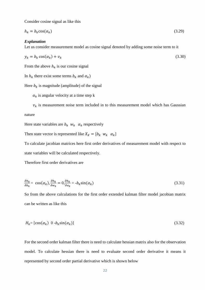
Consider cosine signal as like this

ℎ𝑘𝑘 = 𝑏𝑏𝑘𝑘cos (𝛼𝛼𝑘𝑘) (3.29)

Explanation Let us consider measurement model as cosine signal denoted by adding some noise term to it

𝑦𝑦𝑘𝑘 = 𝑏𝑏𝑘𝑘 cos(𝛼𝛼𝑘𝑘) + 𝑣𝑣𝑘𝑘 (3.30)

From the above ℎ𝑘𝑘 is our cosine signal

In ℎ𝑘𝑘 there exist some terms 𝑏𝑏𝑘𝑘 and 𝛼𝛼𝑘𝑘)

Here 𝑏𝑏𝑘𝑘 is magnitude (amplitude) of the signal

𝛼𝛼𝑘𝑘 is angular velocity at a time step k

𝑣𝑣𝑘𝑘 is measurement noise term included in to this measurement model which has Gaussian

nature

Here state variables are 𝑏𝑏𝑘𝑘 𝑤𝑤𝑘𝑘 𝛼𝛼𝑘𝑘 respectively

Then state vector is represented like 𝑋𝑋𝐾𝐾 = [𝑏𝑏𝑘𝑘 𝑤𝑤𝑘𝑘 𝛼𝛼𝑘𝑘]

To calculate jacobian matrices here first order derivatives of measurement model with respect to

state variables will be calculated respectively.

Therefore first order derivatives are

𝜕𝜕ℎ𝑘𝑘𝜕𝜕𝑏𝑏𝑘𝑘

= cos(𝛼𝛼𝑘𝑘), 𝜕𝜕ℎ𝑘𝑘𝜕𝜕𝑤𝑤𝑘𝑘

= 0,𝜕𝜕ℎ𝑘𝑘 𝜕𝜕𝛼𝛼𝑘𝑘

= -𝑏𝑏𝑘𝑘sin (𝛼𝛼𝑘𝑘) (3.31)

So from the above calculations for the first order extended kalman filter model jacobian matrix

can be written as like this

𝐻𝐻𝑘𝑘= [cos(𝛼𝛼𝑘𝑘) 0 -𝑏𝑏𝑘𝑘sin (𝛼𝛼𝑘𝑘)] (3.32)

For the second order kalman filter there is need to calculate hessian matrix also for the observation

model. To calculate hessian there is need to evaluate second order derivative it means it

represented by second order partial derivative which is shown below

22

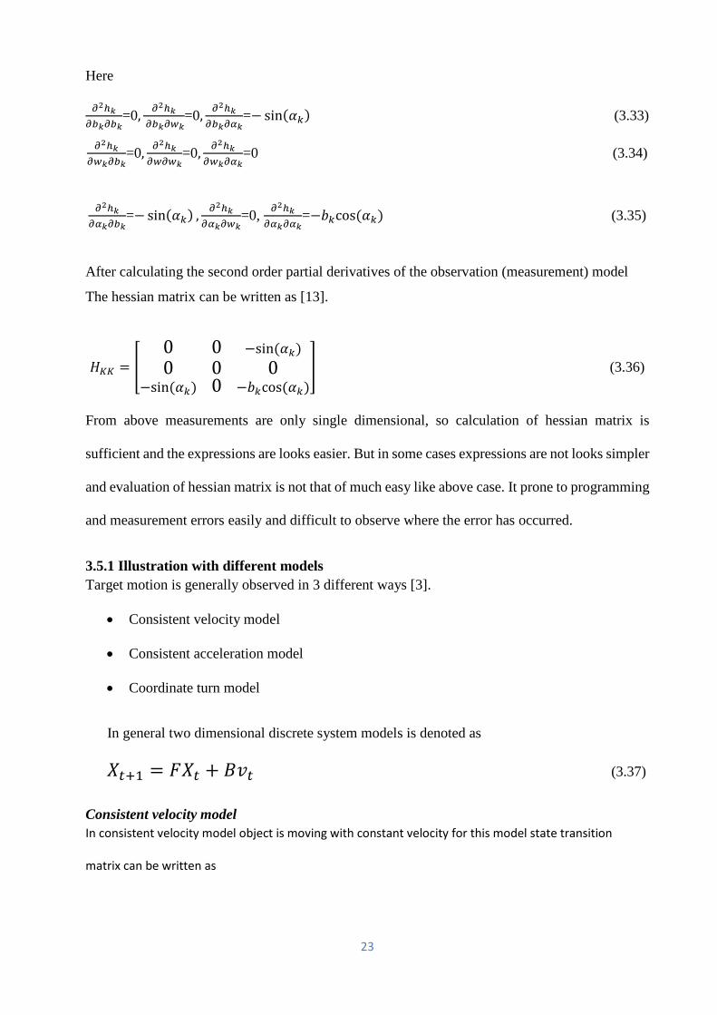
Here

𝜕𝜕2ℎ𝑘𝑘𝜕𝜕𝑏𝑏𝑘𝑘𝜕𝜕𝑏𝑏𝑘𝑘

=0, 𝜕𝜕2ℎ𝑘𝑘 𝜕𝜕𝑏𝑏𝑘𝑘𝜕𝜕𝑤𝑤𝑘𝑘

=0, 𝜕𝜕2ℎ𝑘𝑘𝜕𝜕𝑏𝑏𝑘𝑘𝜕𝜕𝛼𝛼𝑘𝑘

=− sin(𝛼𝛼𝑘𝑘) (3.33)

𝜕𝜕2ℎ𝑘𝑘𝜕𝜕𝑤𝑤𝑘𝑘𝜕𝜕𝑏𝑏𝑘𝑘

=0, 𝜕𝜕2ℎ𝑘𝑘𝜕𝜕𝑤𝑤𝜕𝜕𝑤𝑤𝑘𝑘

=0, 𝜕𝜕2ℎ𝑘𝑘𝜕𝜕𝑤𝑤𝑘𝑘𝜕𝜕𝛼𝛼𝑘𝑘

=0 (3.34)

𝜕𝜕2ℎ𝑘𝑘

𝜕𝜕𝛼𝛼𝑘𝑘𝜕𝜕𝑏𝑏𝑘𝑘=− sin(𝛼𝛼𝑘𝑘) , 𝜕𝜕2ℎ𝑘𝑘

𝜕𝜕𝛼𝛼𝑘𝑘𝜕𝜕𝑤𝑤𝑘𝑘=0, 𝜕𝜕2ℎ𝑘𝑘

𝜕𝜕𝛼𝛼𝑘𝑘𝜕𝜕𝛼𝛼𝑘𝑘=−𝑏𝑏𝑘𝑘cos (𝛼𝛼𝑘𝑘) (3.35)

After calculating the second order partial derivatives of the observation (measurement) model

The hessian matrix can be written as [13].

𝐻𝐻𝐾𝐾𝐾𝐾 = �0 0 −sin (𝛼𝛼𝑘𝑘)0 0 0

−sin (𝛼𝛼𝑘𝑘) 0 −𝑏𝑏𝑘𝑘cos (𝛼𝛼𝑘𝑘)� (3.36)

From above measurements are only single dimensional, so calculation of hessian matrix is

sufficient and the expressions are looks easier. But in some cases expressions are not looks simpler

and evaluation of hessian matrix is not that of much easy like above case. It prone to programming

and measurement errors easily and difficult to observe where the error has occurred.

3.5.1 Illustration with different models Target motion is generally observed in 3 different ways [3].

• Consistent velocity model

• Consistent acceleration model

• Coordinate turn model

In general two dimensional discrete system models is denoted as

𝑋𝑋𝑡𝑡+1 = 𝐹𝐹𝑋𝑋𝑡𝑡 + 𝐵𝐵𝑣𝑣𝑡𝑡 (3.37)

Consistent velocity model In consistent velocity model object is moving with constant velocity for this model state transition

matrix can be written as

23

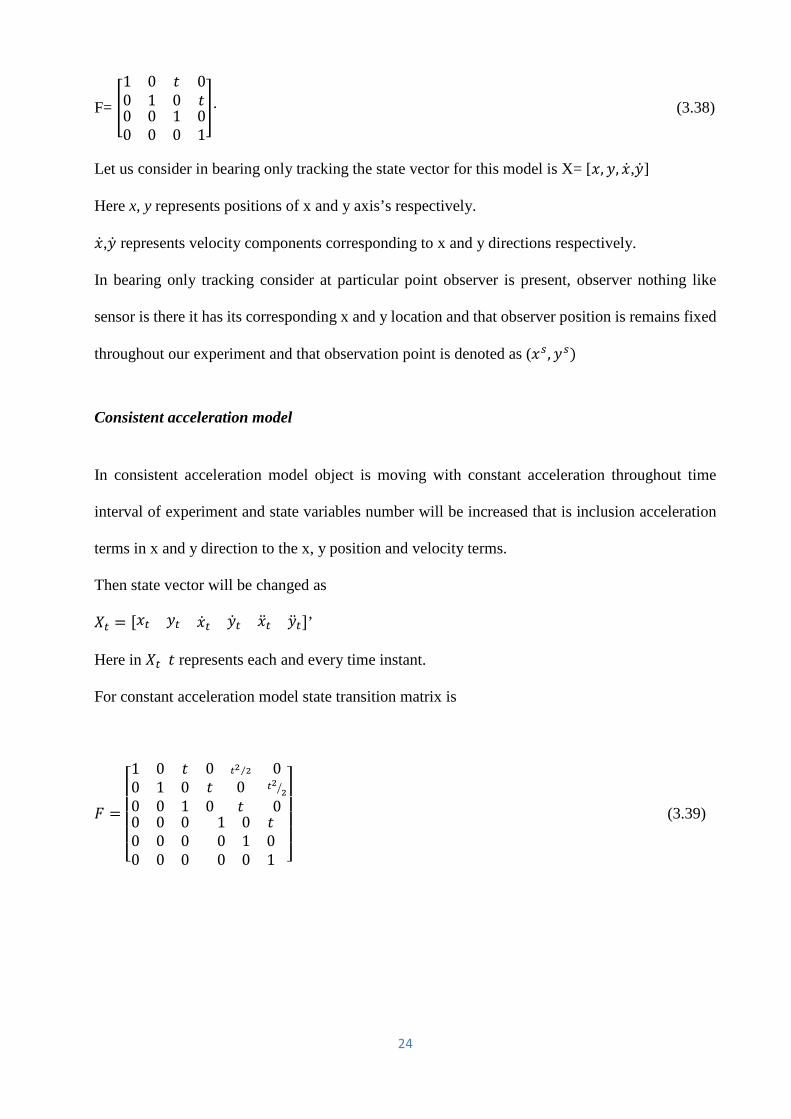
F= �1 00 1

𝑡𝑡 00 𝑡𝑡

0 00 0

1 00 1

�· (3.38)

Let us consider in bearing only tracking the state vector for this model is X= [𝑥𝑥,𝑦𝑦, �̇�𝑥,�̇�𝑦]

Here x, y represents positions of x and y axis’s respectively.

�̇�𝑥,�̇�𝑦 represents velocity components corresponding to x and y directions respectively.

In bearing only tracking consider at particular point observer is present, observer nothing like

sensor is there it has its corresponding x and y location and that observer position is remains fixed

throughout our experiment and that observation point is denoted as (𝑥𝑥𝑠𝑠 ,𝑦𝑦𝑠𝑠)

Consistent acceleration model

In consistent acceleration model object is moving with constant acceleration throughout time

interval of experiment and state variables number will be increased that is inclusion acceleration

terms in x and y direction to the x, y position and velocity terms.

Then state vector will be changed as

𝑋𝑋𝑡𝑡 = [𝑥𝑥𝑡𝑡 𝑦𝑦𝑡𝑡 �̇�𝑥𝑡𝑡 �̇�𝑦𝑡𝑡 �̈�𝑥𝑡𝑡 �̈�𝑦𝑡𝑡]’

Here in 𝑋𝑋𝑡𝑡 𝑡𝑡 represents each and every time instant.

For constant acceleration model state transition matrix is

𝐹𝐹 =

⎣⎢⎢⎢⎢⎡1 0 𝑡𝑡0 1 00 0 1

0 𝑡𝑡2 2⁄ 0𝑡𝑡 0 𝑡𝑡2

2�

0 𝑡𝑡 00 0 00 0 00 0 0

1 0 𝑡𝑡0 1 00 0 1 ⎦

⎥⎥⎥⎥⎤

(3.39)

24

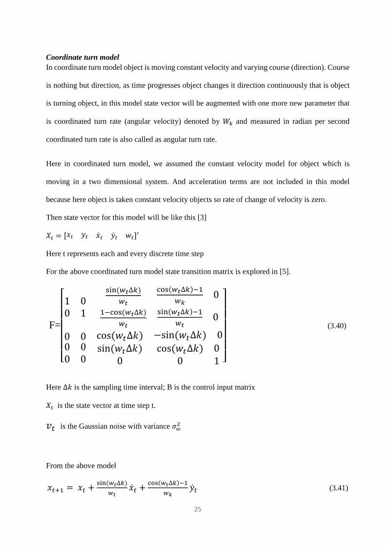
Coordinate turn model In coordinate turn model object is moving constant velocity and varying course (direction). Course

is nothing but direction, as time progresses object changes it direction continuously that is object

is turning object, in this model state vector will be augmented with one more new parameter that

is coordinated turn rate (angular velocity) denoted by 𝑊𝑊𝑘𝑘 and measured in radian per second

coordinated turn rate is also called as angular turn rate.

Here in coordinated turn model, we assumed the constant velocity model for object which is

moving in a two dimensional system. And acceleration terms are not included in this model

because here object is taken constant velocity objects so rate of change of velocity is zero.

Then state vector for this model will be like this [3]

𝑋𝑋𝑡𝑡 = [𝑥𝑥𝑡𝑡 𝑦𝑦𝑡𝑡 �̇�𝑥𝑡𝑡 �̇�𝑦𝑡𝑡 𝑤𝑤𝑡𝑡]′

Here t represents each and every discrete time step

For the above coordinated turn model state transition matrix is explored in [5].

F=

⎣⎢⎢⎢⎢⎢⎡1 00 1

sin (𝑤𝑤𝑡𝑡∆𝑘𝑘)𝑤𝑤𝑡𝑡

cos(𝑤𝑤𝑡𝑡∆𝑘𝑘)−1𝑤𝑤𝑘𝑘

01−cos (𝑤𝑤𝑡𝑡∆𝑘𝑘)

𝑤𝑤𝑡𝑡

sin(𝑤𝑤𝑡𝑡∆𝑘𝑘)−1𝑤𝑤𝑡𝑡

0

0 000

00

cos (𝑤𝑤𝑡𝑡∆𝑘𝑘) −sin (𝑤𝑤𝑡𝑡∆𝑘𝑘) 0sin (𝑤𝑤𝑡𝑡∆𝑘𝑘)

0cos (𝑤𝑤𝑡𝑡∆𝑘𝑘) 0

0 1 ⎦⎥⎥⎥⎥⎥⎤

(3.40)

Here ∆𝑘𝑘 is the sampling time interval; B is the control input matrix

𝑋𝑋𝑡𝑡 is the state vector at time step t.

𝑣𝑣𝑡𝑡 is the Gaussian noise with variance 𝜎𝜎𝜔𝜔2

From the above model

𝑥𝑥𝑡𝑡+1 = 𝑥𝑥𝑡𝑡 + sin (𝑤𝑤𝑡𝑡∆𝑘𝑘)𝑤𝑤𝑡𝑡

�̇�𝑥𝑡𝑡 + cos(𝑤𝑤𝑡𝑡∆𝑘𝑘)−1𝑤𝑤𝑘𝑘

�̇�𝑦𝑡𝑡 (3.41)

25

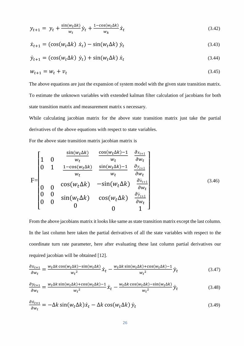
𝑦𝑦𝑡𝑡+1 = 𝑦𝑦𝑡𝑡 + sin (𝑤𝑤𝑡𝑡∆𝑘𝑘)𝑤𝑤𝑡𝑡

�̇�𝑦𝑡𝑡 + 1−cos(𝑤𝑤𝑡𝑡∆𝑘𝑘)𝑤𝑤𝑘𝑘

�̇�𝑥𝑡𝑡 (3.42)

�̇�𝑥𝑡𝑡+1 = (cos(𝑤𝑤𝑡𝑡∆𝑘𝑘) �̇�𝑥𝑡𝑡) − sin (𝑤𝑤𝑡𝑡∆𝑘𝑘) �̇�𝑦𝑡𝑡 (3.43)

�̇�𝑦𝑡𝑡+1 = (cos(𝑤𝑤𝑡𝑡∆𝑘𝑘) �̇�𝑦𝑡𝑡) + sin (𝑤𝑤𝑡𝑡∆𝑘𝑘) �̇�𝑥𝑡𝑡 (3.44)

𝑤𝑤𝑡𝑡+1 = 𝑤𝑤𝑡𝑡 + 𝑣𝑣𝑡𝑡 (3.45)

The above equations are just the expansion of system model with the given state transition matrix.

To estimate the unknown variables with extended kalman filter calculation of jacobians for both

state transition matrix and measurement matrix s necessary.

While calculating jacobian matrix for the above state transition matrix just take the partial

derivatives of the above equations with respect to state variables.

For the above state transition matrix jacobian matrix is

F=

⎣⎢⎢⎢⎢⎢⎢⎡1 00 1

sin (𝑤𝑤𝑡𝑡∆𝑘𝑘)𝑤𝑤𝑡𝑡

cos(𝑤𝑤𝑡𝑡∆𝑘𝑘)−1𝑤𝑤𝑡𝑡

𝜕𝜕𝑥𝑥𝑡𝑡+1

𝜕𝜕𝑤𝑤𝑡𝑡1−cos (𝑤𝑤𝑡𝑡∆𝑘𝑘)

𝑤𝑤𝑡𝑡

sin(𝑤𝑤𝑡𝑡∆𝑘𝑘)−1𝑤𝑤𝑡𝑡

𝜕𝜕𝑦𝑦𝑡𝑡+1

𝜕𝜕𝑤𝑤𝑡𝑡

0 000

00

cos (𝑤𝑤𝑡𝑡∆𝑘𝑘) −sin (𝑤𝑤𝑡𝑡∆𝑘𝑘) 𝜕𝜕�̇�𝑥𝑡𝑡+1


sin (𝑤𝑤𝑡𝑡∆𝑘𝑘)0

cos (𝑤𝑤𝑡𝑡∆𝑘𝑘) 𝜕𝜕�̇�𝑦𝑡𝑡+1


0 1 ⎦⎥⎥⎥⎥⎥⎥⎤

(3.46)

From the above jacobians matrix it looks like same as state transition matrix except the last column.

In the last column here taken the partial derivatives of all the state variables with respect to the

coordinate turn rate parameter, here after evaluating these last column partial derivatives our

required jacobian will be obtained [12].

𝜕𝜕𝜕𝜕𝑡𝑡+1𝜕𝜕𝑤𝑤𝑡𝑡

= 𝑤𝑤𝑡𝑡∆𝑘𝑘 cos(𝑤𝑤𝑡𝑡∆𝑘𝑘)−sin(𝑤𝑤𝑡𝑡∆𝑘𝑘)𝑤𝑤𝑡𝑡2

�̇�𝑥𝑡𝑡 −𝑤𝑤𝑡𝑡∆𝑘𝑘 sin(𝑤𝑤𝑡𝑡∆𝑘𝑘)+cos(𝑤𝑤𝑡𝑡∆𝑘𝑘)−1

𝑤𝑤𝑡𝑡2�̇�𝑦𝑡𝑡 (3.47)

𝜕𝜕𝑦𝑦𝑡𝑡+1𝜕𝜕𝑤𝑤𝑡𝑡

= 𝑤𝑤𝑡𝑡∆𝑘𝑘 sin(𝑤𝑤𝑡𝑡∆𝑘𝑘)+cos(𝑤𝑤𝑡𝑡∆𝑘𝑘)−1𝑤𝑤𝑡𝑡2

�̇�𝑥𝑡𝑡 −𝑤𝑤𝑡𝑡∆𝑘𝑘 cos(𝑤𝑤𝑡𝑡∆𝑘𝑘)−sin(𝑤𝑤𝑡𝑡∆𝑘𝑘)

𝑤𝑤𝑡𝑡2�̇�𝑦𝑡𝑡 (3.48)

𝜕𝜕�̇�𝜕𝑡𝑡+1𝜕𝜕𝑤𝑤𝑡𝑡

= −∆𝑘𝑘 sin(𝑤𝑤𝑡𝑡∆𝑘𝑘)�̇�𝑥𝑡𝑡 − ∆𝑘𝑘 cos(𝑤𝑤𝑡𝑡∆𝑘𝑘) �̇�𝑦𝑡𝑡 (3.49)

26

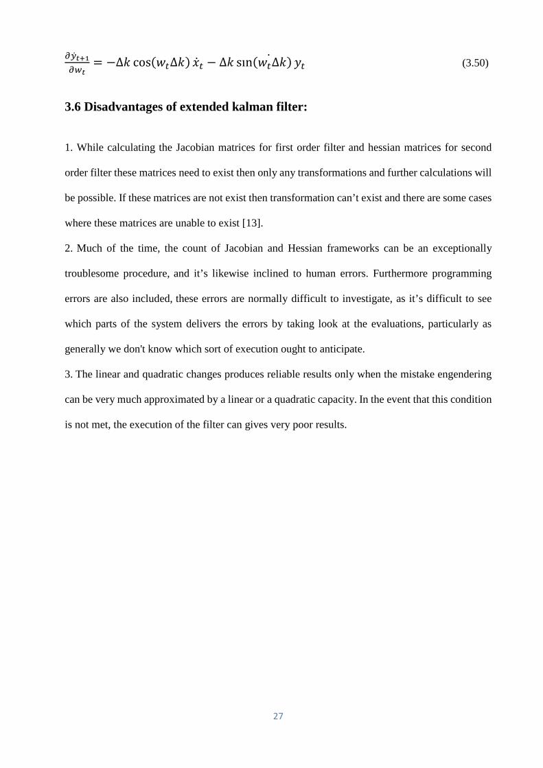
𝜕𝜕�̇�𝑦𝑡𝑡+1𝜕𝜕𝑤𝑤𝑡𝑡

= −∆𝑘𝑘 cos(𝑤𝑤𝑡𝑡∆𝑘𝑘) �̇�𝑥𝑡𝑡 − ∆𝑘𝑘 sın(𝑤𝑤𝑡𝑡∆𝑘𝑘)𝑦𝑦̇ 𝑡𝑡 (3.50)

3.6 Disadvantages of extended kalman filter:

1. While calculating the Jacobian matrices for first order filter and hessian matrices for second

order filter these matrices need to exist then only any transformations and further calculations will

be possible. If these matrices are not exist then transformation can’t exist and there are some cases

where these matrices are unable to exist [13].

2. Much of the time, the count of Jacobian and Hessian frameworks can be an exceptionally

troublesome procedure, and it’s likewise inclined to human errors. Furthermore programming

errors are also included, these errors are normally difficult to investigate, as it’s difficult to see

which parts of the system delivers the errors by taking look at the evaluations, particularly as

generally we don't know which sort of execution ought to anticipate.

3. The linear and quadratic changes produces reliable results only when the mistake engendering

can be very much approximated by a linear or a quadratic capacity. In the event that this condition

is not met, the execution of the filter can gives very poor results.

27

CHAPTER 4 PARTICLE FILTER

28

Chapter4

PARTICLE FILTER

4.1 Introduction From the perspective of useful model on states, the EKF does not ensure an ideal arrangement in

a complicated situation of nonlinearity and non-Gaussian distribution. The particle filter (PF) is an

alternative with competitive performance contrasted with the extended kalman filter.

A few calculations don't adapt to nonlinear state or estimation models and non-Gaussian state or

measured noises, under such sort of circumstances Particle filter is especially adjusted.

Customary routines are taking into account linearized models and Gaussian noise approximate

estimations, so that the Kalman filter can be used. Here major analysis is based on how different

state directions or numerous models can be used to bound the estimations.

In divergence to this, the particle filter estimates the optimal solution based on the system dynamic

model. A well-understood issue with the particle filter is that its performance degrades

immediately when the dimension of the state vector increases. Key hypothetical commitment here

is to apply under estimation procedures prompting that the Kalman filter can be used to evaluate

or take out all position derivatives, and the particle filter is connected with the part of the state

vector containing just the position. Thus, in the particle filters dimensions just depending on the

application, and this is the main measure to get real-time better superior algorithms. When

applying optimal filtering tracking techniques are not tracking the object path there is need to shift

to approximation methods one such kind of approximation method is Monte Carlo methods [15].

Sequential importance sampling uses Monte Carlo methods it approximates the full posteriori

distribution instead of filtering distribution. Sequential importance sampling is the one of major

step in particle filter when optimal filter technique with its corresponding prediction and updating

steps are not sufficient to track the object path. Sequential importance sampling uses some random

particles each particle contains its appropriate weights.

29

4.2 Sequential importance sampling Essential thought of this design is to illustrate the posterior density for an arrangement of weighted

arbitrary samples and to evaluate the parameters of interest depends upon these specimens and

weights [4].

The filtering issue includes the estimation of the state vector at time k, given all the estimations up

to and including time k, which we mean by 𝑧𝑧1:𝑘𝑘. at the point when the estimate and upgrade stage

of the ideal filtering are not tractable accurately, then one needs to turn to estimated systems, one

such technique is Monte Carlo evaluation. Sequential Importance sampling (SIS) is the most

essential Monte Carlo technique utilized for this purpose.

The basic thought in sequential importance sampling is estimating the posterior distribution at time

k that is P (𝑥𝑥0:𝑘𝑘 𝑧𝑧1:𝑘𝑘)⁄ .

In sequential importance sampling it is helpful to consider the full posterior distribution at a time,

instead of the filtering distribution, which is simply the marginal of the full posterior distribution.

In filtering distribution while prediction the state at some time k that is for 𝑥𝑥𝑘𝑘 it required

measurement values from 1: k which is represented like this [13].

P (𝑥𝑥𝑘𝑘 𝑧𝑧1:𝑘𝑘)⁄ where as in full posterior distribution to predict the state 𝑥𝑥0:𝑘𝑘 it requires measurement

values from 1: k which is represented with P (𝑥𝑥0:𝑘𝑘 𝑧𝑧1:𝑘𝑘)⁄ with weighted arrangement of particles

𝑥𝑥0:𝑘𝑘𝑖𝑖 with its corresponding weights 𝑤𝑤𝑘𝑘

𝑖𝑖 where i ranges from 1 to N, and recursively upgrade these

particles to get a close estimation to this posterior distribution.

As the number of samples becomes very large, the SIS filter approaches optimal estimate.

The primary particle set is made by drawing N autonomous acknowledge from p(X0) and allotting

uniform weight 1/N to each of them.

It additionally has two stages.

The expectation comprises of spreading every particle as per the advancement comparison.

The heaviness of every particle is will be changed during the rectification step.

Particle filter tracking algorithm requires five basic steps.

30

4.3 Basic Particle filter model The particle filter gives an approximate solution to an exact model, rather than the optimal solution

to an approximate model. Particle filtering is a general Monte Carlo (examining) technique for

performing derivation in state-space models. Where the state of a system develops in time and data

about the state is acquired by means of noisy estimations measured at each and every time step. In

a general discrete-time state-space, the state of a system model is evolved like this [12].

𝑥𝑥𝑡𝑡 = 𝑓𝑓(𝑥𝑥𝑡𝑡−1,𝑤𝑤𝑡𝑡−1) (4.1)

Here 𝑥𝑥𝑡𝑡 represents the state vector of a system at time t

𝑤𝑤𝑡𝑡−1 is noise vector of system model.

f (.) represents nonlinear state function and it varies with respect to time and illustrates the

reconstruction of new state vector for each and every time instant. State vector 𝑥𝑥𝑡𝑡 is unobservable.

Observation model is represented with ℎ𝑡𝑡 .

Then its measurement vector 𝑧𝑧𝑡𝑡=ℎ𝑡𝑡(𝑥𝑥𝑡𝑡, 𝑣𝑣𝑡𝑡) (4.2)

Here ℎ𝑡𝑡(.) is nonlinear function and it is varies with respect to time which illustrating the

measurement vector and 𝑣𝑣𝑡𝑡 is measurement noise vector.

The major step in particle filtering algorithm is sequential importance sampling are given below.

4.4 Basic algorithm steps • Initialization

• Time update (move particles)

• Measurement update (change weights)

• Degeneracy problem

• Resampling

31

Initialization Here initially we take N random particles assign each particle with equal weights. In this step chose

N random samples (particles) around the initial positons. It means suppose a particular object is

moved in a two dimensional plane chose N random particles in that 2-D plane, here each particle

contains x coordinate and y coordinate and some other parameters depend on the chosen model

[2].

Time update After initializing the particle set, Propagate the particle set according to the process model of target

dynamics.

One-step prediction of each particle

𝑥𝑥𝑡𝑡+1𝑖𝑖 =𝑓𝑓𝑡𝑡�𝑥𝑥𝑡𝑡𝑖𝑖� + 𝑤𝑤𝑡𝑡�𝑥𝑥𝑡𝑡𝑖𝑖� (4.3)

The approximation error decreases as the number of particles grows on increasing.

Measurement update Updating the probability density function based on received measurement value with that update

particle weight [2].

The weights are adjusted using the measurement

𝑤𝑤𝑡𝑡+1𝑖𝑖 = 𝑤𝑤𝑡𝑡

𝑖𝑖𝑝𝑝(𝑦𝑦𝑡𝑡 𝑥𝑥𝑡𝑡𝑖𝑖)⁄ (4.4)

After adjusting the weights all weights will be normalized

𝑤𝑤𝑡𝑡+1𝑖𝑖 = 𝑤𝑤𝑡𝑡+1

𝑖𝑖 /𝛼𝛼 (4.5)

Here 𝛼𝛼 = ∑ 𝑤𝑤𝑡𝑡+1𝑖𝑖𝑁𝑁

𝑖𝑖=1 (4.6)

Here particles can explain measurement gain weight, in this sensor gives bearing angles by taking

N particles and the particles which are far from the true object state will lose weight and the

particles which are nearer to true object state will gain the weight.

32

Degeneracy problem As number of iterations increases, it leads degeneracy problem. Degeneracy problem is that after

some iterations some particles with very less weight an remaining particles carries more weight,

the particles which carries more weight has useful Information and rest of particles are unnecessary

ones.one best solution to the eliminate degeneracy problem is resampling. Degeneracy is generally

measured by effective sample size, it is represented by Neff. [4], [7].

𝑁𝑁𝑒𝑒𝑒𝑒𝑒𝑒 = 1

∑ �𝑤𝑤𝑘𝑘𝑖𝑖�2𝑁𝑁

𝑖𝑖=1 (4.7)

Generally degeneracy is depends on effective sample size 𝑁𝑁𝑒𝑒𝑒𝑒𝑒𝑒 ,if the 𝑁𝑁𝑒𝑒𝑒𝑒𝑒𝑒 value is small that

means it has larger variance in the weights so it has more degeneracy. If 𝑁𝑁𝑒𝑒𝑒𝑒𝑒𝑒 value is high then it

has smaller variance in the weights and so it has less degeneracy problem.

Resampling The resampling can’t perform for each case, resampling will be performed if 𝑁𝑁𝑒𝑒𝑒𝑒𝑒𝑒 falls below

certain threshold value then only we perform resampling in particle filter to increase the accuracy

of estimated state [13]. Threshold values are 2N/3 or 3N/4

There are lot of approaches to perform resampling , out of those systematic resampling is one

approach, in this technique after updating the particles weights with measurement equations we

normalize the particle weights, after that we calculate the cumulative sum of normalized particle

weights, here we generate a some random number in which interval that random number occurred

we use that index value to regenerate the new samples, here we repeat the process until the

regenerated sample number would be equal to that initially generated random particles after

generating the new samples we estimate the new state of the object which we want to track ,and

we reinitialize particles weight to 1/N before going to the second iteration this we repeat over 100

times to find trajectory of object. In this resampling technique in particle filter while resampling

some times while generating random number, if it can’t fall in any cumulative summed interval or

only single particle will be picked sometimes causes sub optimal solution and after some iterations

33

all particles will be divided in to subsets, after some more iterations more particles form a group

but we don’t want all particles to estimate state, here we are using all particles by computing mean

of all particles to estimate new state of object currently also lot of research is going on to

concentrate only on certain number of particles and to neglect remaining unwanted particles,

resampling is great importance in particle filter technique while tracking the nonlinear path of

object [4].

4.5 Sample impoverishment: Resampling will be performed once it will meet effective sample size threshold criteria, while

performing resampling major intension is removal of particles which carries lesser weight and

major concentration is choose the particles which carrying higher weights i.e. particles which

carrying higher weights will be chosen multiple times and get rid of smaller weight particles that

is not picked these particles. While doing like this after some time steps diversity of particles tends

to be decreased and at one particular exceptional case all particles may crumple into a single

particle. This phenomenon is called sample impoverishment problem [4], [13], this will give

contrarily affect to the nature of the estimate.

4.5.1 Regularized particle filter: Regularized particle filter provide the solution to this sample impoverishment problem by

approximating the filtering and posterior distribution with choosing the kernel density estimation

of particles. The most used kernel while density estimation particles is Epanechnikov kernel [4] to

solve the sample impoverishment problem.

34

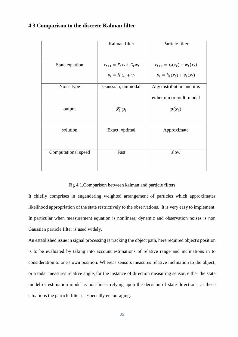
4.3 Comparison to the discrete Kalman filter

Kalman filter Particle filter

State equation 𝑥𝑥𝑡𝑡+1 = 𝐹𝐹𝑡𝑡𝑥𝑥𝑡𝑡 + 𝐺𝐺𝑡𝑡𝑤𝑤𝑡𝑡

𝑦𝑦𝑡𝑡 = 𝐻𝐻𝑡𝑡𝑥𝑥𝑡𝑡 + 𝑣𝑣𝑡𝑡

𝑥𝑥𝑡𝑡+1 = 𝑓𝑓𝑡𝑡(𝑥𝑥𝑡𝑡) + 𝑤𝑤𝑡𝑡(𝑥𝑥𝑡𝑡)

𝑦𝑦𝑡𝑡 = ℎ𝑡𝑡(𝑥𝑥𝑡𝑡) + 𝑣𝑣𝑡𝑡(𝑥𝑥𝑡𝑡)

Noise type Gaussian, unimodal

Any distribution and it is

either uni or multi modal

output 𝑥𝑥𝑡𝑡 ,� 𝑝𝑝𝑡𝑡 𝑝𝑝(𝑥𝑥𝑡𝑡)

solution Exact, optimal

Approximate

Computational speed Fast slow

Fig 4.1.Comparison between kalman and particle filters

It chiefly comprises in engendering weighted arrangement of particles which approximates

likelihood appropriation of the state restrictively to the observations. It is very easy to implement.

In particular when measurement equation is nonlinear, dynamic and observation noises is non

Gaussian particle filter is used widely.

An established issue in signal processing is tracking the object path, here required object's position

is to be evaluated by taking into account estimations of relative range and inclinations in to

consideration to one's own position. Whereas sensors measures relative inclination to the object,

or a radar measures relative angle, for the instance of direction measuring sensor, either the state

model or estimation model is non-linear relying upon the decision of state directions, at these

situations the particle filter is especially encouraging.

35

CHAPTER5 EXPERIMENTAL RESULTS AND DISCUSSION

36

Chapter5

EXPERIMENTAL RESULTS AND DISCUSSION

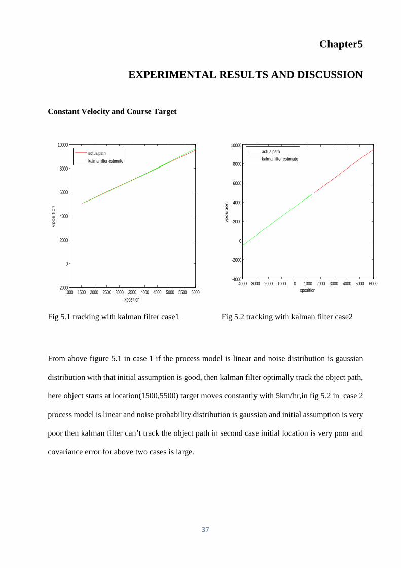
Constant Velocity and Course Target

Fig 5.1 tracking with kalman filter case1 Fig 5.2 tracking with kalman filter case2

From above figure 5.1 in case 1 if the process model is linear and noise distribution is gaussian

distribution with that initial assumption is good, then kalman filter optimally track the object path,

here object starts at location(1500,5500) target moves constantly with 5km/hr,in fig 5.2 in case 2

process model is linear and noise probability distribution is gaussian and initial assumption is very

poor then kalman filter can’t track the object path in second case initial location is very poor and

covariance error for above two cases is large.

1000 1500 2000 2500 3000 3500 4000 4500 5000 5500 6000-2000

0

2000

4000

6000

8000

10000

xposition

ypositio

n

actualpathkalmanfilter estimate

-4000 -3000 -2000 -1000 0 1000 2000 3000 4000 5000 6000-4000

-2000

0

2000

4000

6000

8000

10000

xposition

ypositio

n

actualpathkalmanfilter estimate

37

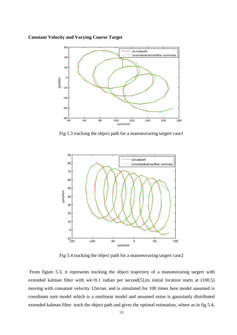
Constant Velocity and Varying Course Target

Fig 5.3 tracking the object path for a manoeuvuring targert case1

Fig 5.4 tracking the object path for a manoeuvuring targert case2

From figure 5.3, it represents tracking the object trajectory of a manoeuvuring targert with

extended kalman filter with wk=0.1 radian per second[5],its initial location starts at (100,5)

moving with consatant velocity 12m/sec and is simulated for 100 times here model aasumed is

coordinate turn model which is a nonlinear model and assumed noise is gaussianly distributed

extended kalman filter track the object path and gives the optimal estimation, where as in fig 5.4,

40 60 80 100 120 140 160 180-80

-60

-40

-20

0

20

40

60

xposition

ypos

ition

actualpathextendedkalmanfilter estimate

-150 -100 -50 0 50 100-10

0

10

20

30

40

50

60

70

80

90

xposition

ypos

ition

actualpathextendedkalmanfilter estimate

38

it represents tracking the object trajectory of a manoeuvuring targert with extended kalman filter

with wk=-0.1 radian per second[5], its initial location starts at (100,5) moving with consatant

velocity 12m/sec and is simulated for 100 times here model asumed is coordinate turn model which

is a nonlinear model and assumed noise is gaussianly distributed extended kalman filter track the

object path and gives the optimal estimation.

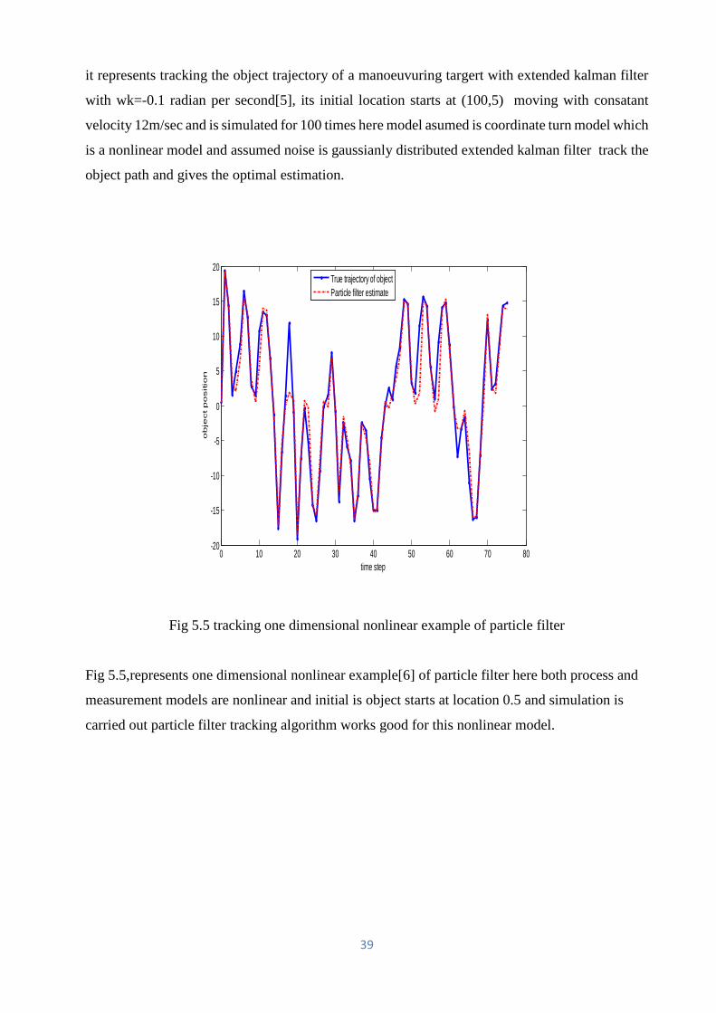
Fig 5.5 tracking one dimensional nonlinear example of particle filter

Fig 5.5,represents one dimensional nonlinear example[6] of particle filter here both process and

measurement models are nonlinear and initial is object starts at location 0.5 and simulation is

carried out particle filter tracking algorithm works good for this nonlinear model.

0 10 20 30 40 50 60 70 80-20

-15

-10

-5

0

5

10

15

20

time step

ob

ject p

ositio

n

True trajectory of objectParticle filter estimate

39

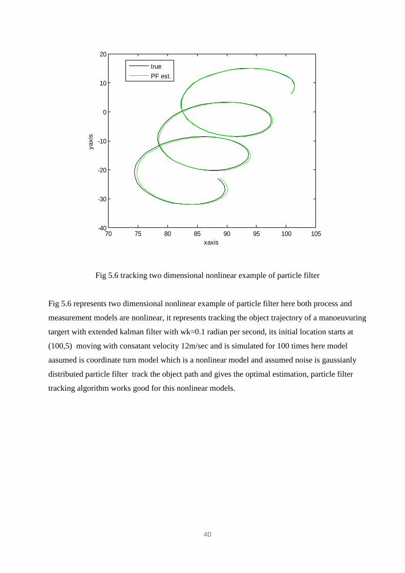
Fig 5.6 tracking two dimensional nonlinear example of particle filter

Fig 5.6 represents two dimensional nonlinear example of particle filter here both process and

measurement models are nonlinear, it represents tracking the object trajectory of a manoeuvuring

targert with extended kalman filter with wk=0.1 radian per second, its initial location starts at

(100,5) moving with consatant velocity 12m/sec and is simulated for 100 times here model

aasumed is coordinate turn model which is a nonlinear model and assumed noise is gaussianly

distributed particle filter track the object path and gives the optimal estimation, particle filter

tracking algorithm works good for this nonlinear models.

70 75 80 85 90 95 100 105-40

-30

-20

-10

0

10

20

xaxis

yaxi

s

truePF est.

40

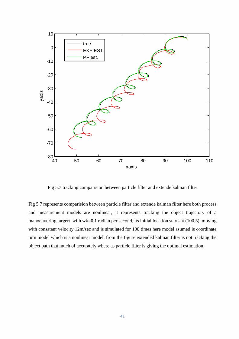
Fig 5.7 tracking comparision between particle filter and extende kalman filter

Fig 5.7 represents comparision between particle filter and extende kalman filter here both process

and measurement models are nonlinear, it represents tracking the object trajectory of a

manoeuvuring targert with wk=0.1 radian per second, its initial location starts at (100,5) moving

with consatant velocity 12m/sec and is simulated for 100 times here model asumed is coordinate

turn model which is a nonlinear model, from the figure extended kalman filter is not tracking the

object path that much of accurately where as particle filter is giving the optimal estimation.

40 50 60 70 80 90 100 110-80

-70

-60

-50

-40

-30

-20

-10

0

10

xaxis

yaxi

s

trueEKF ESTPF est.

41

CHAPTER6 Conclusion and Future Work

42

Chapter6

Conclusion and Future Work We have analyzed various cases of target tracking using extended kalman filter. Based on the

simulation results obtained we have arrived at some major conclusions. Kalman filter gives better

results if the chosen system model is linear model, assumed noise distribution is Gaussian

distribution. Extended kalman filter works well even if chosen system model is nonlinear and noise

distribution is Gaussian distribution and as nonlinearity is more and for non-Gaussian distribution

case it can’t give better results for these kind of cases particle filter gives optimal tracking. The

use of particle filter in the estimation of the object tracking for any kind of system model and noise

seems to have an advantage over the traditional kalman filter based tracking approaches. This is

mainly due to the solution to problem of nonlinearity and non Gaussianity which has been

addressed through the use of the random particles and resampling the use of these object detection

algorithms may further increase the scope of the object path estimation by using some good

resampling techniques as it increases the accuracy of the trajectory.

43

REFERENCES 1. Hue, Carine, J-P. Le Cadre and Patrick Pérez. "Tracking multiple objects with particle

filtering." Aerospace and Electronic Systems, IEEE Transactions on 38, no. 3 (2002): 791-

812.

2. Gustafsson, Fredrik, Fredrik Gunnarsson, Niclas Bergman, Urban Forssell, Jonas Jansson,

Rickard Karlsson, and P-J. Nordlund. "Particle filters for positioning, navigation, and

tracking." Signal Processing, IEEE Transactions on 50, no. 2 (2002): 425-437.

3. Chang, Dah-Chung, and Meng-Wei Fang. "Bearing-Only Maneuvering Mobile Tracking

With Nonlinear Filtering Algorithms in Wireless Sensor Networks."Systems Journal,

IEEE Transactions on 8, no. 1 (2014): 160-170.

4. Arulampalam, M. Sanjeev, Simon Maskell, Neil Gordon, and Tim Clapp. "A tutorial on

particle filters for online nonlinear/non-Gaussian Bayesian tracking."Signal Processing,


5. Radhakrishnan, K., A. Unnikrishnan, and K. G. Balakrishnan. "Bearing only tracking of

maneuvering targets using a single coordinated turn model. International Journal of

Computer Applications on1, no. 1 (2010): 25-33.

6. Gordon, Neil J., David J. Salmond, and Adrian FM Smith. "Novel approach to

nonlinear/non-Gaussian Bayesian state estimation." In IEEE Proceedings (Radar and

Signal Processing), on 140, no. 2 (1993): 107-113.

7. La Scala, Barbara, and Mark Morelande. "An analysis of the single sensor bearings-only

tracking problem." In Information Fusion, IEEE 11th International Conference, (2008): 1-

6.

8. Lin, Yuejin, Fasheng Wang, Yu Han, and Quan Guo. "Bearing-only target tracking with

improved particle filter." In Signal Processing Systems (ICSPS), IEEE 2nd International

Conference on 1, (2010): 331-333.

44

9. Yu, Jinxia, and Wenjing Liu. "Improved Particle Filter Algorithms Based on Partial

Systematic Resampling." IEEE International Conference on Intelligent Computing and

Intelligent Systems on 1, (2010):483-487.

10. Farina, Alfonso. "Target tracking with bearings–only measurements." Signal

processing on78, no. 1 (1999): 61-78.

11. Crouse, David Frederic, R. W. Osborne, Krishna Pattipati, Peter Willett, and Yaakov Bar-

Shalom. "2D Location estimation of angle-only sensor arrays using targets of opportunity."

In Information Fusion (FUSION), IEEE 13th Conference, (2010): 1-8.

12. Panakkal, Viji Paul, and Rajbabu Velmurugan. "Bearings-only tracking using derived

heading." In IEEE Aerospace Conference, (2010):1-11.

13. Hartikainen, Jouni, Arno Solin, and Simo Särkkä. "Optimal filtering with Kalman filters

and smoothers." Department of Biomedica Engineering and Computational Sciences,

Aalto University School of Science: Greater Helsinki, Finland on16 (2011).

14. Zhang, Jinghe, Greg Welch, Gary Bishop, and Zhenyu Huang. "A two-stage Kalman filter

approach for robust and real-time power system state estimation. “Sustainable Energy,


15. Mallick, Mahendra, Mark Morelande, and Lyudmila Mihaylova. "Continuous-discrete

filtering using EKF, UKF, and PF." In Information Fusion (FUSION), IEEE 15th

International Conference, (2012):1087-1094.

45

object tracking using kalman and particle filtering …...object tracking using kalman and particle...

Documents