oberflächenplasmonen-artige resonanzen auf metallischen
TRANSCRIPT

Oberflächenplasmonen-artige Resonanzenauf metallischen Gittern
Dissertation zur Erlangung des Grades
„Doktor der Naturwissenschaften“
am Fachbereich Physik
der Johannes Gutenberg-Universität
in Mainz
vorgelegt von
Maximilian Kreiter
geboren in Neuburg an der Donau
Mainz, 2000

Tag der mündlichen Prüfung: 28. Juni 2000

Surface plasmon-related resonances onmetallic diffraction gratings
submitted to
Fachbereich Physik
Johannes Gutenberg-Universität
Mainz
as a thesis for the degree of
„Doktor der Naturwissenschaften“
by
Maximilian Kreiter
Mainz, 2000


Contents
1 INTRODUCTION ............................................................................................. 1
2 INTRODUCTION TO GRATING- AND SURFACE PLASMON OPTICS......... 3
2.1 Light in matter ......................................................................................................................................3
2.2 The dielectric function of metals .........................................................................................................4
2.3 Reflection of light on a grating ............................................................................................................6
2.3.1 Reflection on a plane multilayer system ..............................................................................................6
2.3.2 Reflection on a grating.........................................................................................................................8
2.3.2.1 Definition of the geometry................................................................................................................8
2.3.2.2 About the electromagnetic problem..................................................................................................9
2.3.2.3 The solution of the electromagnetic problem..................................................................................11
2.3.3 The modelling code ‘oblique’............................................................................................................12
2.4 The surface plasmon resonance as 2-dimensional light ...................................................................14
2.4.1 Grating coupling ................................................................................................................................14
2.4.2 Prism coupling...................................................................................................................................16
2.4.3 The plane interface between two infinite media ................................................................................17
2.4.4 Limitations of the momentum matching approach.............................................................................18
2.4.5 Treatment as purely optical problem .................................................................................................19
3 EXPERIMENTAL........................................................................................... 20
3.1 Preparation of gratings ......................................................................................................................20
3.1.1 Small amplitude .................................................................................................................................20
3.1.1.1 Preparation of the substrate ............................................................................................................20
3.1.1.2 Deposition of photoresist ................................................................................................................21
3.1.1.3 Writing of the grating structure.......................................................................................................21
3.1.1.4 Reactive ion beam etching ..............................................................................................................22
3.1.1.5 Evaporation and removal of the metal coatings ..............................................................................23
3.1.2 Deep gold gratings.............................................................................................................................23
3.1.2.1 Preparation routine .........................................................................................................................23
3.1.2.2 Characterisation ..............................................................................................................................25
3.2 Optical set-up for reflectivity measurements ...................................................................................26
3.3 Optical characterisation of a grating ................................................................................................27

Contents
4 THERMALLY INDUCED EMISSION OF LIGHT FROM A METALLICDIFFRACTION GRATING, MEDIATED BY SURFACE PLASMONS.............. 31
4.1 Introduction ........................................................................................................................................ 31
4.2 Experimental....................................................................................................................................... 32
4.2.1 Sample preparation............................................................................................................................ 32
4.2.2 Emission measurement from the grating at 700°C............................................................................. 32
4.3 Results ................................................................................................................................................. 33
4.3.1 Reflectivity of the grating.................................................................................................................. 33
4.3.2 Angular dependence of the light emission from a gold grating at 700° Celsius ................................ 35
4.3.3 Polarisation of the plasmon enhanced emission ................................................................................ 36
4.4 Conclusion........................................................................................................................................... 37
5 RESONANCES ON DEEP AND OVERHANGING GRATINGS.................... 38
5.1 Introduction ........................................................................................................................................ 38
5.2 Classification of resonances in model calculations .......................................................................... 39
5.2.1 Reflection geometry .......................................................................................................................... 40
5.2.2 Symmetries in the grating profile ...................................................................................................... 40
5.2.3 Shallow gratings ................................................................................................................................ 41
5.2.3.1 The role of the second harmonic of the grating profile................................................................... 43
5.2.3.2 ‘Selection rules’.............................................................................................................................. 44
5.2.4 Deep gratings with mirror symmetry ................................................................................................. 46
5.2.5 Deep, asymmetric gratings ................................................................................................................ 49
5.2.6 A ‘new’ resonance ............................................................................................................................. 49
5.2.6.1 Interaction between the two families of resonances........................................................................ 51
5.2.7 Conclusion......................................................................................................................................... 53
5.3 Experimental results........................................................................................................................... 54
5.3.1 Blazed gratings at ‘normal’ incidence ............................................................................................... 54
5.3.1.1 Etched at 10° .................................................................................................................................. 55
5.3.1.2 Etched at 20° .................................................................................................................................. 58
5.3.1.3 Etched at 30° .................................................................................................................................. 60
5.3.1.4 Etched at 40° .................................................................................................................................. 62
5.3.1.5 Overview on blazed gratings .......................................................................................................... 64
5.3.2 A stationary resonance....................................................................................................................... 66
5.3.3 The deep, symmetric grating ............................................................................................................. 67
5.3.4 The photonic mode density on the surface ........................................................................................ 69
5.4 Conclusion and outlook...................................................................................................................... 70

Contents
6 FLUORESCENCE IN THE FIELD OF COUPLED SURFACERESONANCES ................................................................................................ 72
6.1 Introduction ........................................................................................................................................72
6.1.1 The structure under investigation.......................................................................................................72
6.1.2 Photonic band gaps with monochromatic light ..................................................................................73
6.1.3 Fluorescent dyes in inhomogenous dielectric surroundings...............................................................77
6.1.3.1 The density of states .......................................................................................................................77
6.1.3.2 The modulated interface .................................................................................................................78
6.2 Two models for the fluorescence intensity........................................................................................80
6.2.1 Cross section for the excitation process.............................................................................................80
6.2.2 Cross section of the emission process................................................................................................80
6.2.3 The appropriate averaging procedure ................................................................................................81
6.3 Experimental .......................................................................................................................................82
6.3.1 Sample preparation ............................................................................................................................82
6.3.2 Experimental set-up ...........................................................................................................................83
6.3.3 Additional data treatment...................................................................................................................85
6.4 Results..................................................................................................................................................86
6.4.1 Sample characterisation with reflectivity measurements ...................................................................86
6.4.2 Fluorescence emission in the plane of incidence ...............................................................................87
6.4.3 Detection in the plane of incidence: model calculations....................................................................89
6.4.4 Emission outside the plane of incidence ............................................................................................90
6.5 Selective bleaching..............................................................................................................................92
6.5.1 Observation of the selective bleaching ..............................................................................................93
6.5.2 A new ‘FRAP’ method ......................................................................................................................94
6.6 Conclusion and outlook......................................................................................................................96
7 THE POLARISATION DEPENDENCE OF THE COUPLING TO THESURFACE PLASMON RESONANCE.............................................................. 98
7.1 Introduction ........................................................................................................................................98
7.2 Experimental results...........................................................................................................................99
7.3 Numerical calculations .....................................................................................................................101
7.3.1 Mathematical description of the polarisation...................................................................................101
7.3.2 Comparison between theory and experiment ...................................................................................102
7.3.3 Asymptotic behaviour......................................................................................................................104
7.4 Geometrical discussion .....................................................................................................................105

Contents
7.4.1 Easy geometries............................................................................................................................... 105
7.4.2 Definition of the geometry............................................................................................................... 106
7.4.3 Geometrical interpretation............................................................................................................... 107
7.5 Elliptical polarisation ....................................................................................................................... 109
7.6 Conclusion......................................................................................................................................... 110
8 ABOUT THIN FILM SENSING.................................................................... 112
8.1 Introduction ...................................................................................................................................... 112
8.2 Experimental..................................................................................................................................... 113
8.2.1 Experimental set-up......................................................................................................................... 113
8.2.2 Investigation of a thin film .............................................................................................................. 114
8.3 Evaluation procedures ..................................................................................................................... 115
8.3.1 Rigorous modelling of the grating ................................................................................................... 116
8.3.2 Evaluation by transformation .......................................................................................................... 117
8.4 Conclusion......................................................................................................................................... 120
SUMMARY..................................................................................................... 121
LITERATURE................................................................................................. 123
ABBREVIATIONS.......................................................................................... 130


1 Introduction
Almost 100 years ago, R. W. Wood observed strong, angular dependent variations in theintensity of light that was reflected from an optical metal grating [Woo02]. These effectsare due to the interaction of light with a fundamental excitation of a metal-dielectricinterface. This excitation is characterised by a charge density oscillation in the metal,which is accompanied by an electromagnetic field that extends in both media. Since theenergy is confined to the vicinity of the metal surface, and the conduction electrons of ametal can be treated as a plasma, this excitation is called the surface plasmon resonance.For quite a long period of time, not much progress was made in this field until theavailability of new theoretical and experimental techniques triggered growing interest inthe optics of metal gratings.
Today, many aspects of the optics of metal gratings are well understood, although aquantitative mathematical description of the processes that are involved in theinteraction of light with metal gratings cannot be obtained analytically. The availabilityof computers allowed the development of algorithms that solve this mathematicalproblem numerically, and enabled focusing the attention of contemporary research onthe optics of metal gratings. A short introduction to the basic understanding of „Wood’sanomalies“ and grating optics as established today is given in the second chapter. Thepossibilities offered by numerical modelling are described.
Since lasers have become relatively cheap and easy to handle, optical experiments witha previously unknown precision have become possible. The development of techniquesfor the structuring of surfaces on a sub-micron scale, which were pushed forward by thesilicon technology, allows the preparation of high-quality samples. Details about theexperimental techniques that were explored in this work are described in chapter 3.
A large variety of interesting effects in the context of Wood’s anomalies has now beenstudied both theoretically and experimentally. Many of them are due to the ability of thesurface plasmon resonance to interact not only with light like in Wood’s originalexperiment, but with other forms of energy as well. The strong influence of thegeometry defined by the grating still allows the observation of new and sometimespuzzling effects due to surface plasmons on gratings. The understanding of these effectsis desirable not only from a fundamental point of view, but also because mechanismsthat allow a defined control over the optical properties of a surface promise applicationsin the future. This work is intended as a contribution to gain more insight into the worldof surface plasmons and the ways they exchange energy with other excitations.
The occurrence of Wood’s anomalies is due to an energy transfer from light to thesurface plasmon resonance and from there to thermal energy of the metal. In the fourthchapter, an experiment is presented to prove the possibility of the reverse process:

2 1 Introduction
surface plasmons may be thermally excited and lead to specific light-emission propertiesof a metallic grating.
Another possible channel of energy exchange is the interaction of two surface plasmonswhich is possible on metal gratings. As a consequence, coupled resonances that arequite different from ordinary surface plasmons may exist already on weakly corrugatedmetal surfaces. These resonances are well studied both in theory and experiment[Bar96]. Theoretical studies of the effect of an increased depth of the modulation and astrong asymmetry on the coupled resonances have been reported [Wan98], [Sob98],[Lop98]. They predict a strong change of the coupled resonances as well as new types ofresonances that are supported on sufficiently deep structures. In chapter 5, these effectsare investigated further by model calculations. A new theoretical viewpoint is adapted tocombine the results from literature with some new findings into a consistent picture.These theoretical predictions serve as a basis for the interpretation of the experimentalresults that are in the main focus of this chapter (5).
Both surface plasmons and coupled resonances may exchange energy with electronicexcitations of molecules that are placed in the vicinity of the surface. In the sixthchapter, the influence of the localisation of the electrical field of coupled resonances onthe excitation and emission properties of a fluorescent dye is investigated.
The coupling strength of light to the surface plasmon resonance is strongly dependent onthe polarisation state of the light. In chapter 7, attempts are described to obtain a betterunderstanding of the polarisation dependence for an arbitrary reflection geometry.
Finally, a small contribution is made to the most prominent field of application of thesurface plasmon resonance. Surface plasmon spectroscopy is a method to investigateultra-thin dielectric films on metal surfaces. Due to the difficulties in data analysis,gratings play a negligible role in this field compared to the alternative approach of prismcoupling. In chapter 8, it is shown that gratings are equally well suited for this purposeand an easy evaluation routine is proposed.

2 Introduction to grating- and surface plasmonoptics
In this chapter, some fundamental concepts that build the basis for the followingdiscussions are outlined. The notation for the description of light waves is introduced in2.1, followed by a short discussion of the dielectric function of metals in 2.2. Theelectromagnetic boundary problem of the reflection of light from a grating is describedin 2.3. The surface plasmon resonance is then introduced in the intuitive framework ofmomentum matching in 2.4 and a comparison is made with the alternative approach ofrigorous mathematical modelling.
2.1 Light in matter
For the following, it is necessary to introduce a notation that will be used for thedescription of light waves. For a detailed treatment of electromagnetism, please refer toone out of a huge number of standard textbooks like the book of Jackson [Jac83].Electromagnetic radiation in an isotropic, homogenous medium is described byMaxwell’s equations without source terms.
∇ ⋅ = ∇ × + =
∇ ⋅ = ∇ × − =
E EB
B HD
0
0
∂∂∂∂
t
t
0
0( 2.1 )
Where E is the electrical field, H the magnetic field, D the electrical displacement and Bthe magnetic induction. For this work, the media under investigation were assumed tobe linear. In this case, the full solution of the electromagnetic problem can bedecomposed into independent solutions with a periodicity in time which is given by theangular frequency ω. If such a frequency is fixed by the exciting light, the connectionbetween D and E is given by the dielectric function ε.
( )D E= ⋅ ⋅ε ω ε0 ( 2.2 )
ε0 is the permittivity of vacuum. Similarly, B and H are connected by
( )B H= ⋅ ⋅µ ω µ0 ( 2.3 )
Where µ is the magnetic permeability and µ0 the permeability of free space. Inside ahomogenous and isotropic medium, the solution of Maxwell’s equations as a function oftime t at the point x can be decomposed into plane light waves which are characterisedby their electrical field amplitude E0, the wavevector k and their angular frequency ω.
( ) ( )( )E x E0k x, Ret ei t= ⋅ ⋅ −ω ( 2.4 )

4 2 Introduction to grating- and surface plasmon optics
The orientation of E0 is orthogonal to k. For each pair (ω, k), two mutually orthogonalelectrical field amplitudes may exist, corresponding to two possible polarisations.
Instead of the electrical field, the magnetic field amplitude H0 may be used to describe aplane wave.
( ) ( )( )H x H0k x, Ret ei t= ⋅ ⋅ −ω ( 2.5 )
Both representations contain the full information and one representation may becalculated from the other one with the aid of
H k E
E k H
0
0
00
00
1
1
= ⋅ ×
= ⋅ ×
µ µ ω
ε ε ω
( 2.6 )
Which can be readily seen from ( 2.1 ). For a given angular frequency ω, the modulus ofk is fixed by the dispersion relation
ωµµ εε
2
20 0
2
2
1
k= =
c
n( 2.7 )
With the speed of light in vacuo c and the refractive index n which is defined as theratio of c and the speed of light in matter. In the following, the magnetic permeability µis assumed as 1 which allows to express the modulus of k as a function of the dielectricconstant only.
k = ⋅ = ⋅ = ⋅ω εε µ ε0 0 0 0k k n ( 2.8 )
Where k0, the wavevector of the light wave of the corresponding frequency in vacuo hasbeen introduced. It is often convenient to use the wavelength of the light λ instead ofk, which is defined as
λπ
=⋅2
k( 2.9 )
2.2 The dielectric function of metals
It has been shown in the last section that for homogenous and isotropic media, thedielectric function ε(ω) is needed to describe the response of the material to the externalelectromagnetic field that is produced by the incident light. In this work, the focus lieson two classes of materials that have qualitatively different ε, metals and dielectrics.
In dielectrics, the electrons are bound tightly to the nuclei which leads to a smallpositive and real ε.
2.2 The dielectric function of metals 5
Metals are substances that possess quasi-free electrons which are easily moved by anexternal electrical field. The classical Drude model already allows a good insight intothe response of metals without being forced to deal with the quantum theory of solids. Agood description of the Drude model can be found in many textbooks of solid statephysics, e. g. [Ash76]. The conduction electrons in the metal are assumed to be freelymovable so that they can be accelerated by an externally applied electrical fieldaccording to Newton’s laws. Within a typical time τ, the collision time, they undergo ascattering process after which their propagation direction is completely random and theiraverage velocity depends on the thermal energy of the metal. In this framework, thedielectric constant of a metal as a function of the frequency ω of the applied electricalfield can be derived as
( )ε ωω
ωωτ
= −+
12
2
p
i( 2.10 )
with the plasma frequency ωp which is given as
ωεp
e
e
n e
m2
2
0
= ( 2.11 )
Here, ne is the electron density, e the charge of an electron and me its (effective) mass.Usually, ωp and τ are used to describe the optical response of a metal. These parametersare determined by comparison to experimental values.
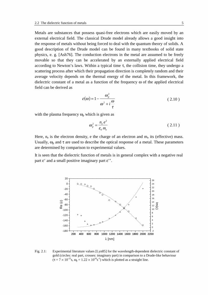
It is seen that the dielectric function of metals is in general complex with a negative realpart ε‘ and a small positive imaginary part ε’’.
200 400 600 800 1000 1200 1400 1600 1800 2000 2200-180
-160
-140
-120
-100
-80
-60
-40
-20
0
20
Im(ε)
Re
(ε)
λ [nm]
200 400 600 800 1000 1200 1400 1600 1800 2000 2200-2
0
2
4
6
8
10
12
14
16
18
20
22
24
26
Fig. 2.1: Experimental literature values [Lyn85] for the wavelength-dependent dielectric constant ofgold (circles: real part, crosses: imaginary part) in comparison to a Drude-like behaviour(τ = 7 × 10-15s, ωp = 1.22 × 10¹⁶s-1) which is plotted as a straight line.
6 2 Introduction to grating- and surface plasmon optics
In Fig. 2.1 the experimentally measured dielectric function of gold in the visible andnear infrared as obtained from literature [Lyn85] is compared to a Drude-like behaviourwith τ = 7 × 10-15 s, ωp = 1.22 × 10¹⁶ s-1. These parameters are chosen for the descriptionof the gold gratings that are investigated in this work. At wavelengths of λ > 650 nm,the Drude model gives a good description of the measured data, at shorter wavelengthsthere is a significant discrepancy. For radiation in the infrared, the large negative valuesof the real part of ε indicate that gold acts as a very good reflector, as it is expected froma metal. In the short-wavelength regime of the visible light, gold is a much worsereflector, instead, there is considerable absorption. This is the reason why gold appearsyellow.
Around λ = 1200 nm there appears a slight discontinuity in ε which is due to the factthat the data were gathered from different experiments. This effect is unphysical and dueto the sometimes rather strong variations in the optical quality of evaporated films as ithas been pointed out by several authors ([Lyn85] and references therein, [Bry91]). Suchan evaporated film is usually composed of microscopic crystallites which areresponsible for some roughness of the surface. Additionally, there may be voids betweenthe grains. Chemical modification of the surface, as it inevitably takes place as soon asthe samples are exposed to air, will have an additional effect on the optical response ofthe metal. Therefore, it is inappropriate to state one ε for gold surfaces that arefabricated by thermal evaporation for a certain wavelength. Instead, the small variationsin the optical response of different samples must be taken into account for a gooddescription of the optical response of metallic surfaces.
2.3 Reflection of light on a grating
In this section, some remarks are made about the electromagnetic problem of a planewave scattered by a grating. Basic concepts of reflection on planar systems are reviewedin (2.3.1) and the reflection on a grating is introduced in (2.3.2). Finally, a briefintroduction in the numerical modelling code that was used for this work is given(2.3.3).
2.3.1 Reflection on a plane multilayer system
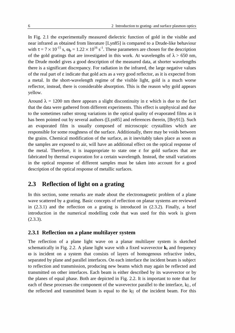
The reflection of a plane light wave on a planar multilayer system is sketchedschematically in Fig. 2.2. A plane light wave with a fixed wavevector ki and frequencyω is incident on a system that consists of layers of homogenous refractive index,separated by plane and parallel interfaces. On each interface the incident beam is subjectto reflection and transmission, producing new beams which may again be reflected andtransmitted on other interfaces. Each beam is either described by its wavevector or bythe planes of equal phase. Both are depicted in Fig. 2.2. It is important to note that foreach of these processes the component of the wavevector parallel to the interface, k, ofthe reflected and transmitted beam is equal to the k of the incident beam. For this
2.3 Reflection of light on a grating 7
reason, the electromagnetic field can be decomposed into two components in each layer,an upward and a downward propagating plane wave which are completely describedeither by their magnetic or by their electrical field.
As it has been pointed out earlier, two orthogonal polarisations are needed for the fulldescription of a plane light wave with a given (ω, k). There is one natural choice of twopolarisations which are not changed with respect to their polarisation state uponreflection and transmission. They are characterised by having one field componentwhich is orthogonal to the plane of incidence which is spanned by the wavevector ki ofthe incident beam and the surface normal: If the incident beam has an (E- or H- ) fieldcomponent which is confined to this direction, the same holds for all transmitted andreflected beams. Therefore, the choice of the electrical field in the case of transverseelectric polarisation (TE) as basis of the description of the entire problem and of themagnetic field in the case of transverse magnetic polarisation (TM) is particularly easy.
ki
kt
kd
k
kr
ku
Fig. 2.2 Schematic representation of reflection on a planar 3-layer system. Each plane wave isrepresented by its wavevector k. The subscripts stand for ‘incident’ (i), ‘reflected’ (r),‘downward’ (d), ‘upward’ (u), ‘transmitted’ (t). The in plane component k is equal for allthese contributions. The thin lines depict the planes of constant phase.
For example, consider the TE case. In each layer, only the complex amplitudes of thedownward propagating wave and the upward propagating wave, Ed and Eu must bedetermined to obtain the electromagnetic field distribution in the entire system as wellas the reflected and transmitted intensities. In the case of TM polarisation, an equivalentargument holds for the magnetic field. The transfer matrix algorithm (See e.g. [Kar91])allows the determination of Eu and Ed for the case TE and of Hu and Hd for TM

8 2 Introduction to grating- and surface plasmon optics
polarisation in each layer. An arbitrary polarisation is described as linear superpositionof the two fundamental polarisations. The local field distributions and the intensities andpolarisation states of the reflected and transmitted intensities are calculated by linearsuperposition of the individual response of the system to TM and TE light.
2.3.2 Reflection on a grating
2.3.2.1 Definition of the geometry
In this work, only relief gratings in one dimension are considered as schematicallydepicted in Fig. 2.3.
zx
Λ
Fig. 2.3: Schematic representation of a multilayered grating.
Again, we deal with layers with a homogenous refractive index and thickness, but allinterfaces are now periodically modulated in an identical way. These interfaces aredescribed as the functional dependence z(x).
( ) ( )z x z x A i xi ii
= + = ⋅°
⋅ ⋅ +
=
∞
∑ΛΛ
sin360
0
ϕ( 2.12 )
Where Λ is the grating pitch or period of the grating. Due to the periodicity this functionmay be decomposed into a Fourier representation with amplitudes Ai and phases ϕi.
The parameters that are required to describe the reflection geometry of a planeelectromagnetic wave on such a structure are schematically sketched in Fig. 2.4.
The polarisation of the incident light is described as a superposition of TM and TEpolarised light with components of the electrical field parallel to the two orthogonal unitvectors pTM and pTE. If linearly polarised light is considered, the polarisation may bedescribed by a real angle ϕ where
( ) ( )( )E p p p p0 TE TM TE TM0 0= ⋅ + ⋅ = +E E ETE TM
0 sin cosϕ ϕ ( 2.13 )

2.3 Reflection of light on a grating 9
kg
k
ϕ
θ
Ψ
xy
zpTMk i
pTE
Fig. 2.4: Definition of the parameters that are used to describe reflection of a plane electromagneticwave on a relief grating.
The co-ordinate system is by definition fixed relative to the symmetry axes of thegrating. The z-axis is chosen along the surface normal, y parallel and x perpendicular tothe grating grooves. The wavevector ki of the incident beam is in the most general casedescribed by the wavelength λ of the incident light, the polar angle θ which denotes thetilt of ki relative to the surface normal, and the azimuthal angle Ψ which defines thecounterclockwise rotation of the plane of incidence relative to the x-axis, seen along theincident beam (in the sketch, Ψ ≈ -20°). The wavevector of the incident beam may bewritten in terms of θ and Ψ.
( ) ( )( ) ( )
( )k i = ⋅ ⋅
⋅⋅
−
k0 εθθ
θ
sin cos
sin sin
cos
ΨΨ ( 2.14 )
The vectorial representation of the fundamental polarisations will be treated to somemore detail in chapter 7. The reciprocal grating vector kg is defined as
k g =
=
k g
0
0
2
0
0
πΛ
( 2.15 )
2.3.2.2 About the electromagnetic problem
An introduction to the electromagnetic theory of gratings is given in the book edited byPetit [Pet80]. The Floquet-Bloch theorem is of fundamental importance for the optics ofgratings. It states that for a periodically modulated interface, the electrical field outsidethe modulated area due to the reflected beam can be described as
( ) ( ) ( )E x t p pTMk x
TEk x, = ⋅ ⋅ + ⋅ ⋅
=−∞
∞− −∑ E e E e
TM
m
TE
mm
m
i t m i tω ω ( 2.16 )

10 2 Introduction to grating- and surface plasmon optics
With complex amplitudes of the electrical field in the two fundamental polarisations.Additional contributions, the higher diffracted orders are introduced which arecharacterised by the integer m, the order of the diffracted wave. The wavevector of them’th diffracted order, km is defined as
( ) ( ) ( )k m =
+ ⋅
± ⋅ − − + ⋅
k m k
k
n k k k m k
xi
g
yi
yi
xi
g0
2 2 2
( 2.17 )
where the superscript i denotes the Cartesian components of the incident beam and kg isthe modulus of the reciprocal grating vector. The expression describing the z-componentis readily derived from the x and y component with the aid of the dispersion of light (2.8 ). It is important to note that this decomposition into plane waves is valid only forthose z which belong to planes normal to z that lie completely in one medium (‘regionoutside the grating grooves’). The validity of this expansion inside the grooves, theRayleigh assumption, is an approximation which may only be used for shallow gratings(See [Pet80], [Kaz96]).
The additional contributions to the electromagnetic field that are introduced by thepresence of a surface relief grating are depicted schematically in Fig. 2.5.
ki
m = 0
m = -1
m = +1
kg
Fig. 2.5: Schematic sketch of the diffracted orders that are introduced by a relief diffraction grating.
In addition to the specular beam (m = 0) that would be there even without a modulationof the interface, new waves are introduced to the system which have an in-planewavevector which is modified by a multiple integer of the reciprocal grating vector.They may be plane waves with a wavevector that has got only real components if the z-component in equation ( 2.17 ) is the square root of a positive number. This is the casefor the -1st diffracted order in the example given above. The plane waves are drawn in

2.3 Reflection of light on a grating 11
the sketch as dashed lines. For the +1st diffracted order, the situation is different. Here,the large k leads to a negative denominator in the root in ( 2.17 ), as a consequence, kz
is purely imaginary. In this case the exponential function in ( 2.16 ) consists of aperiodically oscillating part in x and y direction and an exponential part along z. Thesewaves are bound to the surface, their intensity decays with a decay length which is givenby kz−1. This property is expressed in the sketch by lines that become thinner withincreasing distance from the sample. Because the intensity of these waves vanishes withincreasing distance from the surface they are called evanescent (from lat. evanescere,vanish, die away) waves.
In general, the solution of the electromagnetic problem of a plane wave falling on arelief grating cannot be decomposed into linearly independent orthogonal waves that areexcited either by TM or by TE polarisation like on a plane interface. Only for Ψ = 0°these solutions remain independent. This geometry is called the classical mount, othergeometries are referred to as conical incidence.
2.3.2.3 The solution of the electromagnetic problem
For the calculation of the response of a grating to illumination with a plane wave, it isnecessary to find the amplitudes of all the diffracted orders by application of theboundary conditions to the electrical and magnetic field on the (curved) interface. Onlynumerical approaches to this problem are known. There are several mathematicalconcepts to solve this problem which are reviewed in the book of Petit [Pet80] and byMaystre [May82]. An overview over some more recent developments can be found inthe paper of Barnes et al. [Bar96]. Even today, new mathematical approaches are beingdeveloped [Pla99].
In this work a computer code was used which is based on the work of Chandezon et al.[Cha82] and was progressively refined by various scientists. In the original version thiscode allows the calculation of the optical response of a multilayer system where theindividual isotropic layers are separated by interfaces of equal shape in the classicalmount.
Elston et al. [Els91] extended the approach of Chandezon to conical incidence.
Cotter et al. [Cot95] changed the method of transfer matrices to the ‘scattering matrixapproach’, a concept which was developed by Li [Li94b] which enhances the numericalstability and therefore applicability of the algorithm.
Preist et al. [Pre97] made the calculation of highly blazed and even overhanginggratings possible by introducing a transformation to a non-orthogonal co-ordinatesystem which is parametrised by the ‘obliquity angle’ θob. The Cartesian co-ordinates x,z of a point which has the oblique co-ordinates xob and zob is given by
( )( )
z z
x x z
ob ob
ob ob ob
= ⋅
= + ⋅
sin
cos
θ
θ( 2.18 )
12 2 Introduction to grating- and surface plasmon optics
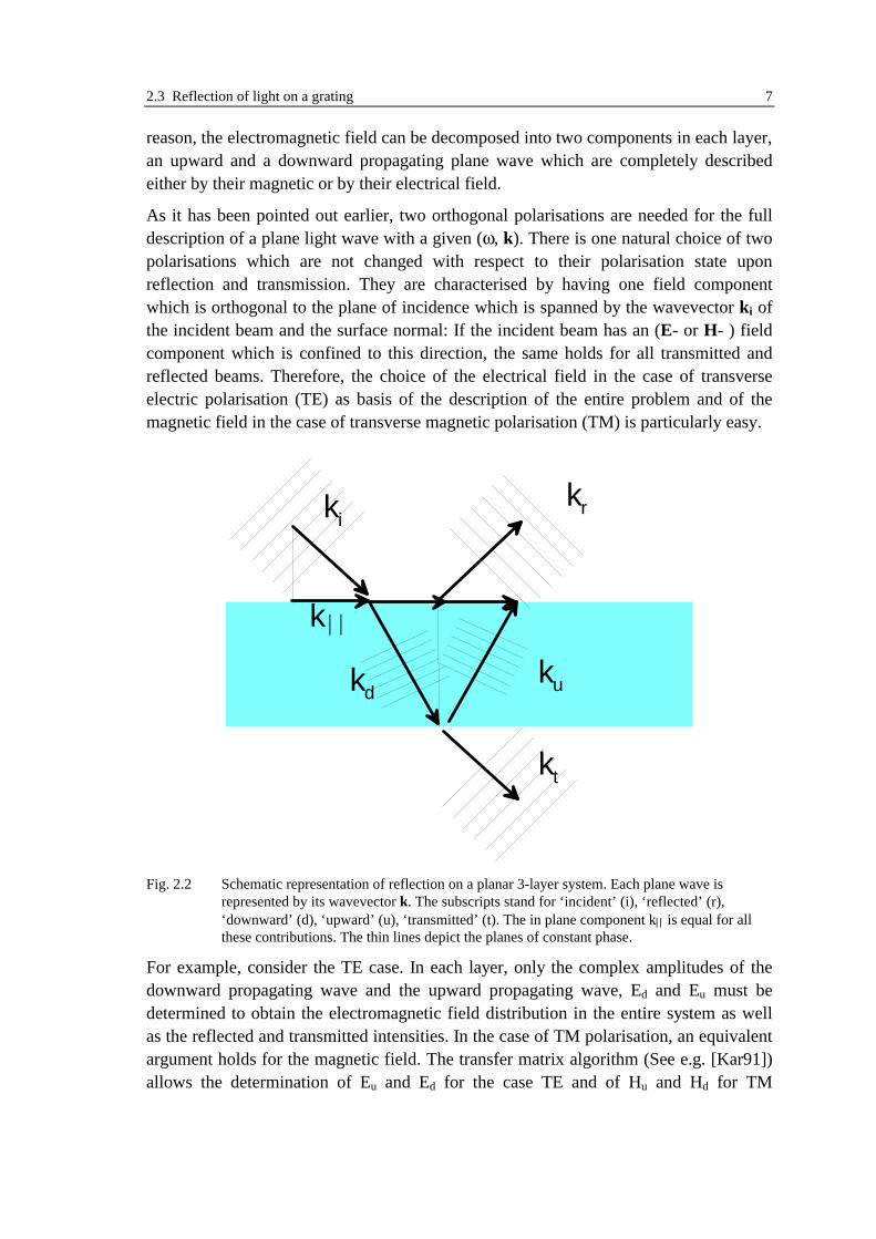
An illustrative example is given below (Fig. 2.6), the form of a pure sine function in anoblique co-ordinate system with θob = 55° is plotted in real space. It is obvious that thisline cannot be represented as a function in the Cartesian co-ordinate system becausethere y(x) is not unique.
0 200 400 600 800 1000 1200 1400 1600-400
-200
0
200
400
600 0 400 600
600
400
200
0
200
z [n
m]
x [nm]
Fig. 2.6: The Cartesian representation of a sine function with a period of Λ = 700 nm and an amplitudeof A1 = 400 nm in a non-orthogonal co-ordinate system with θob = 55°. The grid indicateslines of constant zob and xob in the oblique system.
Other extensions of this modelling routine which are not used in this work are reportedas the inclusion of anisotropic materials [Har96], an infinite periodicity in z-direction[Tan98] as well as the investigation of a multilayer system with different grating shapes[Pre95]. The extension to structures that are modulated in two dimensions has beendemonstrated, too [Har96b].
2.3.3 The modelling code ‘oblique’
It is far beyond the scope of this introduction to explain the algorithms that are used forthe modelling of the optical response of such a grating structure. As an alternative to thecitations given above, a detailed description of the underlying mathematics is given bythe author of the numerical modelling code [Wan99].
For the application of the numerical code it is necessary to specify which parameters areused to describe the electromagnetic boundary problem for the numerical evaluation. Inaddition, the results that are calculated by the code must be specified. This informationis put together in Table 2.1.

2.3 Reflection of light on a grating 13
Table 2.1: Input- and output- parameters of the numerical modelling code ‘oblique’
Input Parameters Output Parameters
Grating Profile Far field
→ Pitch Λ → Intensities of all the outgoing beams, Im
→ Amplitudes Ai, Phases ϕi → Phases of all the outgoing beams, ϕm
→ Obliquity angle θob Near field
Reflection geometry
→ Polar angle θ
→ Magnetic field distribution Hx(x,y,z),Hy(x,y,z), Hz(x,y,z)
→ Azimuthal angle Ψ
→ Polarisation (TM/TE)
→ Electrical field distribution Ex(x,y,z),Ey(x,y,z), Ez(x,y,z)
→ Wavelength λ
Layer system
→ Thickness of all layers except 1st andlast
→ Dielectric function, fixed (ε’, ε’’) orDrude (ωp, τ)
The grating profile is described by the pitch Λ, the obliquitiy angle θob and theamplitudes Ai and phases ϕi of the Fourier representation. Only a few Fouriercomponents are usually needed to get a reasonable agreement of the model calculationwith nature.
The incident beam is specified by its wavelength λ, the propagation direction which isgiven by θ and Ψ and its polarisation which may be either TM or TE. Since thepolarisations are defined relative to the plane of incidence, they have a non-trivial formin the co-ordinate system which is fixed relative to the grating. Arbitrary polarisationsare deduced from those as linear superposition as discussed in Chapter 7.
The dielectric properties of each layer are expressed by its dielectric constant ε. It can bechosen either as fixed or a wavelength-dependence according to the Drude model maybe assumed (compare section 2.2). In the latter case, the collision time τ and the plasmafrequency ωp must be specified. The thickness must be given for each layer except thefirst and the last one which are assumed to extend to infinity.
The physical quantities calculated by the program are the intensities (square of thecomplex amplitudes) of the two orthogonal polarisations of all diffracted orders whichare not evanescent. All diffracted orders are used to calculate the electrical and magneticfield distributions in real space which are complex vector functions that vary in 3dimensions.

14 2 Introduction to grating- and surface plasmon optics
2.4 The surface plasmon resonance as 2-dimensional light
In this section, a phenomenological introduction to the surface plasmon resonance ispresented. From experimental observations on gratings (2.4.1) and special planarsystems (2.4.2), the existence of a surface wave on the metal-dielectric interface can bededuced. This wave has a well defined in-plane wavevector for a given angularfrequency ω. Some properties of the surface plasmon resonance in the easiest case of aflat interface between an infinitely thick metal and an infinitely thick dielectric arediscussed in 2.4.3. Finally, after revealing some limitations of the approach of a planesurface wave (2.4.4), the importance of the alternative approach of rigorous modelling ishighlighted in 2.4.5. The aim of this chapter is to give an introduction to the basics ofthe surface plasmon resonance. Special properties that are investigated in this work areintroduced in the corresponding chapters.
2.4.1 Grating coupling
In 1902, Wood observed in the classical mount that under certain angles of incidencethe intensity of the light reflected from a metallic diffraction grating is significantlyreduced at certain wavelengths for TM polarisation [Woo02]. A qualitative explanationof these observations was given by Fano [Fan41] almost 40 years later who postulated‘superficial waves which are excited by the impinging wave on the surface of thegrating’. In Fig. 2.7, the measured reflectivity of a metal grating is shown as a functionof the polar angle θ of the incident light. The reflectivity is defined as the fraction of theincident intensity which is specularly reflected.
-5 0 5 10 15 20 25 30 35 40 45 50 55 60 65
0.2
0.4
0.6
0.8
1.0
Re
flect
ivity
θ [°]
Fig. 2.7: Reflectivity of a gold grating with Λ = 773.6 nm at a wavelength of λ = 632.8 nm and TMpolarised light in the classical mount (Ψ = 0°).

2.4 The surface plasmon resonance as 2-dimensional light 15
Clearly, the reflectivity is reduced at θ = 13.7° and at θ = 35.5°. Furthermore, forθ = 10.6° and for θ = 39.4°, sharp kinks are observed. These kinks are due to thetransition of a diffracted order from a plane to an evanescent wave. It is straightforwardto show with the aid of equation ( 2.17 ) that the -2nd diffracted order is a propagatingwave only for θ > 39.4° while the +1st diffracted order is a propagating wave only forθ < 10.6°. These kinks are referred to as ‘pseudocritical edges’ because they areoriginating, like the critical edges in the reflectivity from an interface separating twomedia of high and low refractive index from the transition of a light beam from a planeto an evanescent wave. The two minima can be explained by the existence of anelectromagnetic wave which is excited whenever a diffracted order has an in-planewavevector of a given length. From the data, the in-plane component of this wave isdetermined as k = 1.055 k0. The resonance at θ = 13.7° is excited by the evanescent+1st diffracted order while the resonance at θ = 35.5° is due to the evanescent -2nd
diffracted order. At this point it can be readily seen that this electromagnetic wave isbound to the interface (evanescent) because with a k > k0 equation ( 2.17 ) immediatelyyields a purely imaginary z-component of the wavevector.
In the conical mount (Ψ ≠ 0), this approach of momentum matching in the surface planeis equally well suited to describe the position of the pseudocritical edges and the surfaceplasmon resonance minima. In Fig. 2.8, measured positions of surface plasmon-relatedminima and pseudocritical edges are compared to the positions that are obtained bymomentum matching of the diffracted order to the surface plasmon resonance with afixed k = 1.055 × k0.
7060504030201000
20
40
60
80
θ [°]
ψ [°
]
0 20 40 60 80 100
0
20
40
60
80
100
120
140
160
180
m = -1
m = +2
m = -2
m = +1
Ψ[°
]
θ[°]
Fig. 2.8: Left: Measured TM-reflectivity of a gold grating as a function of θ and ΨRight: Positions of Wood anomalies as obtained from momentum matching and from themeasurement: surface plasmons (measured: open circles, geometrical: thick line) andpseudocritical edges (measured: full squares, geometrical: thin line)
A good agreement between measurement and calculation is observed with respect to theposition of the surface plasmon resonance and the pseudocritical edge. The depth of theminimum cannot be predicted by momentum matching as well as the vanishing of the

16 2 Introduction to grating- and surface plasmon optics
dip for Ψ = 90°. These effects will be treated in some detail in chapter 7. It should benoted, too, that the momentum-matching approach fails for the resonances at Ψ = 90°even if they are excited. A deeper analysis of this ‘photonic band gap’ is given inchapter 5.
2.4.2 Prism coupling
An alternative way to excite the surface plasmon resonance on a planar metal surface isbased on the momentum enhancement of light in a high-index medium to establishcoupling to the long k of the surface plasmon resonance.
high index mediumε = 3.24 (prism)
metalε = -13 + 1.2 i
k,plasmon
k0
low index mediumε = 1 d = 650 nm
ki
θ
0 20 40 60 80 100
0.0
0.2
0.4
0.6
0.8
1.0
Re
flect
ivity
θ [°]
Fig. 2.9: Left: sketch of the planar system and the wavevectors involved in prism coupling in the Otto-geometry.Right: the θ-dependent reflectivity that is obtained from a model calculation assumingλ = 632.8 nm and the layer system as indicated in the sketch.
Otto [Ott68] demonstrated that coupling to the surface plasmon resonance is possiblewith the aid of a 3-layer-system as depicted in Fig. 2.9 (left). Resonant excitation of thesurface plasmon is achieved on the metal surface through the gap of low refractive indexwhere the two evanescent fields overlap. At a certain angle of incidence θ, theprojection of the wavevector of the incident beam matches the plasmon wavevector andcoupling between the two electromagnetic waves is established. On the right, the θ-dependent reflectivity as obtained from a model calculation based on a transfer-matrixcalculation is shown. A deep and sharp minimum is observed that is due to coupling tothe surface plasmon. Since the high index medium must be a prism for geometricalreasons, this method to excite surface plasmons is referred to as ‘prism coupling in theOtto configuration’. The precise values of dielectric constants and thickness are chosenfor illustrative purposes, different values are common.

2.4 The surface plasmon resonance as 2-dimensional light 17
high index mediumε = 3.24 (prism)
metalε = -13 +12 id = 50 nm
kplasmon
k0
low index medium(ε = 1)
ki
θ
0 20 40 60 80 100
0.0
0.2
0.4
0.6
0.8
1.0
Ref
lect
ivity
θ [°]
Fig. 2.10: Left: sketch of the planar system and the wavevectors involved in prism coupling in theKretschmann-geometry.Right: the θ-dependent reflectivity that is obtained from a model calculation.
Kretschmann [Kre71] found a similar behaviour of the structure that is depicted in Fig.2.10. Again, coupling to the surface plasmon resonance leads to a well pronouncedminimum in the reflectivity. Here, the surface plasmon is excited through a thin metalfilm. Please refer to [Aus94], [Kno97], [Kno98], Kno91], [Rae88], [Sam91], [Yea96] or[Bur74] for a deeper treatment of prism coupling.
2.4.3 The plane interface between two infinite media
In the last two sections it became evident that the existence of the surface plasmonresonance which is an electromagnetic surface excitation with a well-definedwavevector for a given frequency is very helpful for the understanding of the results ofoptical experiments1. In some sense, the z-component of this resonance may bedisregarded which leads to the interpretation of the surface plasmon as 2-dimensionallight. A modulated interface between two infinitely thick media may be regarded to afirst approximation as flat with the modulation as a perturbation. Similarly, in the prismcoupling set-up one may treat the finite thickness of the gold (Kretschmann-configuration) or of the air gap (Otto configuration) as perturbation to the case of twoinfinitely thick media. The mathematics for this system is relatively easy which makes itworth discussing some properties of the plasmon resonance in this simple model case.
The existence of the surface plasmon resonance as an electromagnetic wave can bederived by an analysis of Maxwell’s equations on a planar metal-dielectric interface. Itturns out that there is an electromagnetic wave which decays exponentially away fromthe interface both into the dielectric and the metal with a magnetic field distributionsaccording to equation ( 2.5 ) where the magnetic field vector H0 is parallel to the
1 Some recent extensions of this concept to a corrugated metal film of finite thickness are reported by
Schröter et al. [Sch99].

18 2 Introduction to grating- and surface plasmon optics
interface, and the in-plane component k of the wavevector is given by the dispersionrelation:
( ) ( ) ( )( ) ( )k k m d
m d
ωε ω ε ωε ω ε ω
=⋅+0
( 2.19 )
where the subscript ‘m’ stands for metal and ‘d’ for dielectric. For the detailedderivation of this equation, please refer to the literature e. g. the book of Raether[Rae88]. One important observation is made on this dispersion relation: in order toobtain an in-plane wavevector k which exceeds k0, it is necessary to have dielectricconstants with opposite sign. This is the case in metals due to the ‘plasma-likebehaviour’ of the electron gas (compare section 2.2). Because of that and theconfinement to the interface, the term ‘surface plasmon’ was chosen.
One way to prove the existence of this resonance experimentally without a grating or byintroducing a finite thickness of one of the two media is the scattering of electrons froma metal surface [Rae88]. The transferred energy and momentum can be determined andit turns out that one possible scattering process is the excitation of surface plasmonquanta. This shows that, even when it is not detectable by optical means, the surfaceplasmon resonance is a fundamental excitation of the surface.
2.4.4 Limitations of the momentum matching approach
In the last section, the surface plasmon resonance was treated as a fundamentalexcitation of the metal-dielectric interface. The angular positions of minima in thereflectivity can be explained by resonant coupling to the incident light, momentummatching is achieved either by the addition of reciprocal grating vectors in the case ofgrating coupling or by enhancement of the wavevector of the incident light in a highindex medium. This picture is very helpful for the intuitive understanding of thecoupling to the surface plasmon. A quantitative treatment of reflectivity measurementsin this framework is plagued with the following difficulties:
• It is not clear how the coupling strength of a grating with a given amplitude or of agold film of a certain thickness can be deduced.
• There are more processes involved than the conversion of light to the surfaceplasmon. The reversed process must be taken into account as well as all otherchannels of energy transfer between excitations. For example the observation thatin Kretschmann-configuration the reflectivity minimum does not coincide with themaximum field enhancement on the metal-dielectric interface [Lieb99] [Bar85]can be explained by considering the coherent superposition of different channelsof energy transfer. This approach has been developed to some extend byHerminghaus et al. [Her94] for plane metal surfaces but a quantitative descriptionsturns out to be very difficult with this approach.

2.4 The surface plasmon resonance as 2-dimensional light 19
• The surface plasmon itself is altered by the introduction of a grating or bychanging the thickness of one layer. This effect may be treated in a perturbativeway but complicates the calculations significantly. The explanations of effects thatare due to the self-coupling of surface plasmons like the ‘photonic band gap’ willbe complicated within this framework.
2.4.5 Treatment as purely optical problem
A quantitative description of the optical response of a planar multilayer system ispossible with the aid of the transfer matrix algorithm (compare [Kar91]). Only thegeometry of the problem and the dielectric constants of the involved materials arerequired. For a grating, numerical methods like the extended Chandezon method(compare 2.3.2.3) can be applied. The measured reflectivity curves, includingreflectivity minima which can be assigned to the excitation of the surface plasmonresonance, are well reproduced by the appropriate choice of parameters (comparechapter 3). It should be noted that it is not necessary to know about the existence of asurface resonance beforehand for the quantitative modelling, the minima appear‘automatically’. So, this approach, which considers the reflection process as a purelyoptical problem is fully applicable for a quantitative description of the experimentalfindings. Nevertheless, the picture of a resonance of well defined dispersion which maybe excited by light is much more intuitive. Both approaches should therefore be used forthe explanation of experimental data in order to combine mathematical accuracy withintuitive insight.

3 Experimental
Some background information about the experimental techniques that are important forthe investigation of the interaction of light with modulated metal surfaces is given inthis chapter. First, the preparation of metallic grating surfaces is described in 3.1.Slightly different approaches are used to obtain shallow structures with a depth-to-pitchratio smaller than 0.1 and deep structures. The experimental set-up that was used torecord the optical response of the gratings is introduced in 3.2. Finally, in section 3.3,some remarks are made concerning the optical characterisation of the grating surface.Some special experimental techniques which are applied only in the experiments whichare dealt with in one chapter will be described there.
3.1 Preparation of gratings
3.1.1 Small amplitude
The major steps in the production routine for shallow gold gratings are depicted in Fig.3.1. The grating structure is written into photoresist by a holographic technique andtransferred into the surface of a glass slide by standard photolithographic procedures.Only a thin gold layer is responsible for the optical properties of the surface. This goldlayer may be removed and the substrate may be reused several times.
glass
spin-coating photoresist
evaporation
ion-milling
write &develop
cleaninggold
Fig. 3.1: The production of shallow gold gratings. The amplitudes of the gratings are not to scale.
In the following subsections, details of the different steps are explained. The completesample preparation was done in the cleanroom of the Max-Planck-Institut fürPolymerforschung in Mainz (class 100).
3.1.1.1 Preparation of the substrate
A fused silica slide (Hellma, optical quality) is carefully cleaned by the followingprocedure:
• 10 × rinsing in purified water (Milli-Q, Millipore)
• 15 minutes cleaning in the ultrasonic bath in a solution of 2% detergent(Hellmanex, Hellma) in purified water

3.1 Preparation of gratings 21
• 15 × rinsing in purified water
• 5 minutes cleaning in the ultrasonic bath in ethanol (Fluka)
• Drying of the slides in a flow of nitrogen. For optimum results the ethanol shouldwithdraw from the glass surface as a compact lamella.
3.1.1.2 Deposition of photoresist
As a next step, a photoresist layer (Shipley microposit) is deposited on the glass surfaceby spin coating. In order to enhance the adhesion of the photoresist to the surface, theglass surface is pre-treated with liquid hexamethyldisilazane (‘Primer’, Shipley). Bestresults were obtained by heating the glass close to the evaporation temperature of theprimer. The glass slide is put on the spin-coater and the surface is completely wettedwith the primer solution. After 30 s the remaining solution is removed by spinning thesample at moderate speed (2000 rpm). Immediately afterwards the photoresist is appliedto the resting sample. The thickness of the photoresist layer is tuned by dilution in‘thinner’ (Shipley) and by adjusting the rotation frequency of the spin-coater. Forsymmetric grating structures a thickness around 100 nm is favourable because of theenhanced stability of the photoresist. For highly asymmetric gratings, though, it isnecessary to use a very thin photoresist layer (40-50 nm). Thick photoresist films aredried for 30 minutes under vacuum at 95° C (softbake). For very thin films, this step isnot necessary.
3.1.1.3 Writing of the grating structure
In this work, a method for the fabrication of relief gratings in photoresist was used thatwas first reported by Mai et al. [Mai85]. The sample is mounted in the optical set-upthat is depicted in Fig. 3.2. The beam of a TE-polarised He-Cd laser (λHeCd = 442 nm,Optilas) is passing through a spatial filter which produces a parallel beam which doesnot show significant variation in intensity in the vicinity of the optical axis over an areaof a few cm2.
mirror
sam
ple
spatial filter θ
lasera b
Fig. 3.2: The optical set-up that is used to prepare holographic gratings.
While one half of the beam (ray a) is incident directly on the sample, the other half (rayb) is reflected by a mirror. Depending on the phase difference between these twopossible paths there may be either constructive or destructive interference on the sample

22 3 Experimental
surface. Ideally, the intensity distribution on the grating surface is sinusoidal with aperiod Λ that is given by
( )Λ =⋅λ
θHeCd
2 sin( 3.1 )
as it can be shown with elementary geometry. The polar angle θ is defined as the anglebetween the optical axis and the normal of the sample surface (compare Fig. 3.2).
Care must be taken to avoid the interference effects with laser light which is reflectedfrom the backside of the glass slide. Black adhesive tape on the backside of the samplehelps to reduce the intensity of this unwanted light.
In the intensity maxima of this interference pattern, the photoresist undergoes aphotochemical reaction, which leads to solubility of the material in the developingreagent while photoresist that was not illuminated remains insoluble. Developing thisstructure leads to a surface relief grating in the photoresist. A coherent photoresist layerwith a modulation of the surface may be obtained by exposing the sample only shortly tothe laser light or by choosing a short developing time. This structure is needed for theproduction of highly asymmetric gratings. Longer times lead to separated stripes ofphotoresist with areas of bare substrate in-between. For the production of symmetricgratings, such structures are required.
3.1.1.4 Reactive ion beam etching
By exposure to an ion beam, the photoresist grating is transferred into the glasssubstrate. A sketch of the ion mill (Roth & Rau) is found in Fig. 3.3.
cathode(+1050V)
anode(1200 V) acceleration grid
(-1000 - 0 V)
ions
e-, Ar-
neutraliser
cathode
sample(ground)
θetch
dischargechamber(ground)
screen grid
Fig. 3.3: Sketch of the ion mill.
The ion mill supplies accelerated ions that bombard the sample surface. In detail thisworks as follows:
A dilute mixture of gases (O2 and CF4) is flowing into the discharge chamber. Electronswhich are emitted by the cathode are accelerated towards the anode and by scattering

3.1 Preparation of gratings 23
gas molecules are ionised. So, inside the anode ring, a plasma is built which lies at ahigh positive potential. The numbers given in the sketch are for illustrative purpose andvalues different from those are common. Positive ions are accelerated towards thescreen grid which lies on ground potential. A second grid (acceleration grid) where apotential between 0 V and -1000 V may be applied allows focusing of the beam. The ionbeam finally reaches the sample (which is at ground potential) with a kinetic energycorresponding to the potential of the anode. The neutraliser adds negative ions andelectrons to the beam in order to avoid charging of the sample. By adjusting theorientation of the sample relative to the ion beam an anisotropy may be introduced to theetching process.
For symmetric gratings the etching angle θetch is adjusted to 0° (normal incidence of theion beam). For the shallow asymmetric gratings θetch up to 80° were used to obtain thehigh anisotropy that is needed for the measurements that are presented in chapter 6. Bestresults for the highly asymmetric, shallow gratings were obtained by etching for 1minute at θetch = 0° first (ablation of 20 nm photoresist and 40 nm glass) beforeswitching to the high θetch. The asymmetric gratings are etched long enough that nophotoresist remains on the glass. They are therefore immediately ready for the next step.On the symmetric gratings there are some residues of photoresist which are removed inwarm acetone.
The combination of reactive gases (O2 and CF4) is optimised for the etching of fusedsilica where a mechanical ablation (sputtering) and a chemical etching by the radicalsthat are deduced from the reaction gases takes place. As a consequence, the etchingefficiency depends on the partial pressures of gases for glass. The ablation of othermaterials as gold or chromium is a pure sputtering process and no influence of thechemistry of the gases could be observed.
3.1.1.5 Evaporation and removal of the metal coatings
A gold layer (Balzers, purity 99.99%) is thermally evaporated onto the sample in acommercial evaporation chamber (Balzers). By choosing a thickness exceeding 150 nm,the gold layer can be assumed as infinitely thick for the optical analysis. The adhesion ofthe gold to the silica substrate may be enhanced by a thin (3 nm) layer of chromium(Balzers, purity 99.9%) between gold and glass which is thermally evaporated in thesame chamber. After the experiment, the gold layer is removed with aqua regia (mixtureof HCl and HNO3 in the ratio 3:1). The chromium layer is removed with an aqueoussolution of ammonium cerium (IV) nitrate (Aldrich, purity 99 %, 12 g in 50 ml water).
3.1.2 Deep gold gratings
3.1.2.1 Preparation routine
In order to obtain gratings that are as deep as possible, the standard process for theproduction of holographic gratings that was described in the previous section had to be

24 3 Experimental
modified. A schematic overview over the different steps of the production routine isshown in Fig. 3.4.
Standard microscope slides (obtained from Menzel) are carefully cleaned (compare3.1.1.1) and by thermal evaporation a thin chromium layer followed by a ca. 1000 nmthick gold layer and another chromium layer with a thickness of 200 nm are depositedon the sample. The first chromium layer enhances the adhesion of the gold to thesurface, the second is chosen as masking material because it is very resistive to ion-etching processes (The etching rate in Au is roughly 4-5 times higher than inchromium). For the production of highly asymmetric gratings, a large contrast in etchingresistance between mask and the material where the structure is finally written isneeded. Such thick gold layers are required because the gratings have a very highamplitude and, in order to simplify the evaluation, the gold should be thick enough toallow the assumption of an infinite thickness. The evaporation materials were obtainedfrom Balzers with a purity of 99.99 % (Au) and 99.9 % (Cr).
gold
photoresistchromium
interfering beams
wet - etching
Reactive Ion Beam Etching
(θetch = 0°)
Reactive Ion Beam Etching
(θetch > 0°)
Reactive Ion Beam Etching
(θetch = 0°)
Reactive Ion Beam Etching
(θetch > 0°)
Fig. 3.4: Sketch of the different steps for the preparation of the deep gold gratings.
This system serves as support for a photoresist film (Shipley Microposit) of 100 nmthickness which is deposited by spin coating (compare 3.1.1.2) without application ofprimer. A holographic grating is written into the photoresist. The development is longenough to ensure that the photoresist structure has already evolved from a coherent layerto separated stripes. Subsequently, the sample is exposed to an aqueous solution ofammonium cerium (IV) nitrate (Aldrich, 99 %, 12 g in 50 ml water) for 70 seconds.This step serves to transfer the photoresist structure into the chromium. As a next step,the sample is treated by reactive ion beam etching (see 3.1.1.4) until the chromium iscompletely etched away. By choosing the etching angle θetch (angle between thedirection of the ion beam and the surface normal of the grating, compare Fig. 3.3)between 0° (normal incidence) and 40°, gratings with different degrees of asymmetrycan be obtained. The orientation of the grating is chosen so that the ion beam isorthogonal to the grating grooves.

3.1 Preparation of gratings 25
To some extend, the grating amplitude can now be decreased by etching further into thepure gold grating.
3.1.2.2 Characterisation
The gratings that were produced this way were characterised with a scanning electronmicroscope (leo 912) in order to obtain as much information about the shape of thegrating profile as possible. The samples are broken along a line orthogonal to the gratinggrooves from the backside of the substrate. This is followed by focusing the objective ofthe electron microscope onto the freshly cleaved edge at an angle of 5° relative to thenormal of the cleaved surface. This allows the surface profile to be read from theseimages without applying a stretching factor. Fig. 3.5 shows the grating profile fordifferent etching angles.
θetch = 0° θetch = 10° θetch = 20°
θetch = 30° θetch = 40°
Fig. 3.5: Electron micrographs of grating structures that were obtained by etching under the angles thatare indicated on the graphs. The grating period is Λ = 700 nm.
It is clearly seen that with this technique, it is possible to obtain gold gratings with adepth-to-pitch ratio close to 1. The grating shape can be varied from a mirror symmetricprofile when etched under 0° to overhanging structures when etched under 40°. Fromimages like these, the grating shape had to be extracted. This was done by drawing acurve by hand into the images that reproduced the surface profile as good as possible.This curve was then transformed into discrete points z(x). A least squares-fit to theaverage of five data sets that were obtained on different grating peaks gave finally theparameters for the description of the profile. The first three amplitudes Ai and phases ϕi
of the Fourier sum and the oblique angle θob (compare chapter 2) were obtained thatway. One major disadvantage of this characterisation technique should be mentioned:the sample must be destroyed to allow a measurement. Therefore, it was not possible to

26 3 Experimental
characterise the identical sample for different exposure times in the reactive ion beametcher.
3.2 Optical set-up for reflectivity measurements
The reflectivity of the gratings was measured for linearly polarised light as a function ofthe wavelength λ, the polarisation ϕ and angle of incidence (θ, Ψ) of the incoming light.
θ
laser
monochromator
light source
objective
detector
Ψ
polariserchopper
Fresnel rhomb
sample
Fig. 3.6. Sketch of the optical set-up for reflectivity measurements.
In Fig. 3.6 the optical experimental set-up is shown schematically. The light of a Xenonlight bulb (Osram Xenophot, 300 W in a Müller SVX 1530 housing) is collimated by anobjective onto the slit of a grating monochromator (Chromex 250 SM). After its exitslit, a lens turns the light into a parallel beam. Linear polarisation is fixed by a Glan-Thompson polariser (OWIS) and the polarisation plane can be deliberately rotated witha Fresnel rhomb (Bernhard Halle). Two pinholes select the components of the beamwhich are close to the optical axis and are therefore almost parallel. A laser beam(HeNe, λ = 632.8 nm, Uniphase 1125P) is coupled into the optical path with aremovable mirror. It serves both for the optical alignment in experiments where thewavelength of the incident light is varied and as a light source for reflectivitymeasurements with monochromatic light.
The sample is fixed on a goniometer (sample-goniometer) (Huber) that allows variationof the polar angle θ. For θ = 0°, the sample surface is orthogonal to the incident beam.The axis of this goniometer coincides with the sample surface. A second goniometer(Ψ-goniometer) (Spindler & Hoyer) is mounted on top of the first one. For θ = 0°, itsaxis is coincident with the incoming beam. It allows the variation of the azimuthal angleΨ which is counted as clockwise rotation of the sample viewed along the incident beam

3.3 Optical characterisation of a grating 27
and which is 0° when the grating grooves are perpendicular to the drawing plane. Bycomparison with Fig. 2.4, the geometry may become clearer.
The specularly reflected light is focused onto the detector by a lens with a focal lengthof 50 mm. These two components are mounted on a third (detector- ) goniometer(Huber) on an optical bench. The axis of this goniometer coincides with the one thatvaries θ. It tracks the direction of the reflected beam in θ/2θ geometry. The detector iseither a silicon-photodiode (for λ = 500 to 1100 nm) or a germanium-photodiode (forλ = 1000 to 1800 nm)
The incoming beam is chopped at 1234 Hz and the voltage signal from thephotodetector is analysed by a lock-in amplifier (EG&G, model 7260) with thisfrequency as reference signal. The three goniometers, the Fresnel rhomb and themonochromator are controlled by a PC. The output of the lock-in amplifier is also fed tothis PC.
The spectral intensity for the two fundamental polarisations of the incoming beam isrecorded by adjusting the detector goniometer to 180° and removing the sample. Inorder to measure reflectivities of the sample the readings of the lock-in in a reflectionexperiment are normalised to this reference. While the output power of the laser isrelatively stable over time, there are significant drifts in the intensity spectrum of thecombination of white light source and monochromator. Therefore, those referencespectra must be taken at the same day as the reflected intensities.
3.3 Optical characterisation of a grating
The parameters that determine the optical response of a metal grating without additionalcoatings are the grating period Λ, the dielectric constant ε of the gold and the shape ofthe grating profile which is expressed as a Fourier sum with phases ϕi and amplitudesAi.
The grating period is easily determined in the ‘Littrow mount’ which is defined as theposition of the grating where the -1st diffracted order is propagating back in the directionof the incident beam. In this case, obviously Ψ = 0° holds and basic geometry showsthat the grating period can be calculated from the Littrow angle θLit by the followingequation:
( )Λ =⋅
λθ2 sin Lit
( 3.2 )
where λ denotes the wavelength of the incident light.
The remaining parameters are determined by a least square fit to the data. Thisprocedure is illustrated by taking the data set as an example that was already used toillustrate coupling to the surface plasmon in chapter 2.4.1.

28 3 Experimental
-5 0 5 10 15 20 25 30 35 40 45 50 55 60 65
0.2
0.4
0.6
0.8
1.0
Measurement Selected for fit Calculation
Ref
lect
ivity
θ [°]
Fig. 3.7: Reflectivity of a grating with a pitch of Λ = 773.6 nm which was illuminated with a TM-polarised HeNe laser (λ = 632.8 nm). The fit yields ε = -10.37 + i 1.014, A1 = 19.82 nm,A2 = 5.98 nm, ϕ1 = 40.3°, A3 = 2.97 nm, ϕ2 = 46°.
It turns out that 3 Fourier components are sufficient to obtain a reasonable fit to themeasured points. A computer program, based on the ‘oblique’ code calculates the sumof squares of the difference between the measured reflectivities of up to 20 selectedpairs (R, θ) and the modelled reflectivities based on a certain set of parameters. Byvariation of the fitting parameters within a pre-defined range, the set of parameterswhich leads to a minimum deviation from the measured results is stepwise approached.For details of the fitting algorithm, the reader is referred to the thesis of Wanstall[Wan99].
In the case of a grating profile which was etched symmetrically, the phases of the higherFourier components may only take discrete values. For a ϕ1 which is chosen as 0, ϕ2
may equal either 90° or 270°, ϕ3 may be 0° or 180° and so on (compare chapter 5).Therefore, this parameter should be kept constant during the fit. The real value may thenbe determined by comparing the results of fitting routines with the different possiblechoices. Alternatively, ϕ2 may be determined by mapping of the photonic band gapwhich is composed of two coupled resonances. On symmetric gratings there is alwaysone of the two coupled resonances suppressed, which one is determined by ϕ2. For moreinformation regarding the photonic band gap, the reader is referred to chapter 5 andchapter 6. It is important to note that the set of parameters that gives an optimumdescription of the experimental results does not necessarily yield exactly the real shape

3.3 Optical characterisation of a grating 29
of the grating profile. This is illustrated in Fig. 3.8. It is not very reasonable that such aprofile would be obtained by the preparation technique that was described above.
This difference between the real grating profile and the one that gives an optimumdescription of the data can be interpreted as an effect of the roughness of the samplewhich is not accounted for in the numerical modelling code. An overestimation of thehigher harmonics of the grating profile leads to short-pitch modulation of the profile. Itseems that this periodic roughness has a similar effect on the reflectivity as randomscattering.
-200 0 200 400 600 800 1000 1200 1400 1600
-60
-50
-40
-30
-20
-10
0
10
20
30
z [n
m]
x [nm]
Fig. 3.8: Grating profile as it is deduced from the fit to the data (thick line). The individual Fouriercomponents are plotted below the sum profile as thin lines.
This interpretation is supported by the analysis of the impact of variation of the fittingparameters on the quality of the fit. By model calculations under variation of theseparameters, it turns out that small changes in A1, A2 and ϕ2 will lead to a significantdecrease of the quality of the fit. Especially in Ψ = 90° geometry (compare Chapter 5)the gap between the coupled resonances as well as their relative strength dependstrongly on these parameters. Variations in ϕ3 do not lead to significant changes. Thisallows the conclusion that the first two components of the Fourier representation reflectthe real grating profile. The third order as an additional fitting parameter is necessary fora good model calculation, it accounts for both the real effects of the third harmoniccomponent and for roughness effects. Because of the weak influence of ϕ3 on thereflectivity, the surface profile as it is reconstructed, including the third component,deviates from the real geometry.
It should be mentioned that to a good approximation the amplitude of the i’th order ofthe grating profile is responsible for the coupling to the surface plasmon resonance ini’th diffracted order. For this reason, on gratings with bigger Λ where surface plasmonresonances in higher diffracted orders can be observed, the determination of more

30 3 Experimental
Fourier components of the grating profile is possible by a fit to the reflectivity.Similarly, it is difficult to obtain much information about the profile of a grating with ashort pitch as it is used for the experiments that are described in chapter 4 and chapter 8.Detailed descriptions of the fitting process as well as comparisons to real gratingprofiles that were determined independently by scanning probe methods can be found inliterature [Woo95], [Wat97], [Wat97b].

4 Thermally induced emission of light from ametallic diffraction grating, mediated by surfaceplasmons
4.1 Introduction
It is well known that good light absorbers are good emitters when they are heated; ablack body shows the highest output of radiation at a given temperature. This fact iscalled Kirchhoff’s law and is treated in most standard textbooks on physics like[e. g. Ger82].
On metal gratings, due to the resonant excitation of surface plasmons a strong angularvariation of the reflectivity is observed. The fraction of light which is absorbed uponreflection may vary between about 10 % outside resonance up to ideally 100 % when thesurface plasmon resonance is excited. As a consequence, a reciprocal angular variationin emission is expected. Observed under the angle of vanishing reflectivity due tosurface plasmon excitation, the metal grating should have the emission properties of ablack body for the corresponding wavelength. Fig. 4.1 shows how the underlyingprocesses may be qualitatively understood in a simplified picture. In a reflectionexperiment, some fraction of the light is lost due to ‘direct absorption’ of the incidentradiation. This contribution is independent from the existence of a grating. In the long-wavelength regime of the visible light, less than 10% of the incident light is lost in thisdecay channel. Under certain angles an additional strong process may be observedwhich is sketched in Fig. 4.1 (a) the light is transformed to a surface plasmon by addinga reciprocal grating vector. The energy of the surface plasmon is then finallytransformed into heat by absorption within the gold. When the thermal energy of themetal is high enough, the same processes in the reversed direction may have asignificant probability as shown in Fig. 4.1 (b): the thermal energy may be transformeddirectly into plane electromagnetic radiation which is not expected to show a strongangular variation. This is the glowing that would be observed from a not-modulatedgold surface as well. Additionally some of the surface plasmon states are populatedaccording to Boltzmann’s law and these electromagnetic waves may pick up the pseudo-momentum corresponding to a reciprocal grating vector and leave the sample as light.This contribution is expected to be strongly angle-dependent.

32 4 Thermally induced emission of light...
(a)
incomingwave
reflected wave
surface plasmon
kg
(b)
kg
surface plasmon
plasmonmediated direct
Fig. 4.1: Processes of energy transfer between light and thermal energy of a metal grating.(a) Loss of energy in a reflection experiment due to intermediate excitation of the surfaceplasmon resonance. Additionally, direct absorption may take place.(b) Processes that lead to light emission from a hot sample. Either direct emission or theintermediate excitation of the surface plasmon may take place.
It is the goal of this chapter to demonstrate this effect experimentally. First, details ofthe sample preparation are given and the experimental set-up is described. Then, themeasured angle dependent emission is compared to the reflectivity at the correspondingwavelength.
4.2 Experimental
4.2.1 Sample preparation
A grating with a pitch of Λ = 484.9 nm was fabricated on a fused silica substrate asdescribed in chapter 3.1. A gold film with a thickness of 140 nm was thermallyevaporated onto the grating. A thin (3 nm) chromium layer between the glass and thegold prevented dewetting of the gold at temperatures up to 700° C. The grating wasoptically characterised by a reflectivity measurement in the classical mount as describedin chapter 3.2.
4.2.2 Emission measurement from the grating at 700°C
The experimental set-up that was used to record the intensity of light at certainwavelengths emitted from the gold grating is shown schematically in Fig. 4.2. Thegrating is fixed on a turning stage which contains a heating unit that is used to adjust the

4.3 Results 33
sample temperature to roughly 700°C. The grating grooves are perpendicular to thedrawing plane (classical mount, Ψ = 0°). To avoid chemical reactions, the chamber isevacuated to a pressure of 10-3 mbar.
θsample~ 700 °C
chopper
aperture
photo-detector
interferencefilter
10-3 mbarlensL1
lensL2
polariser
Fig. 4.2: Experimental set-up for angle-resolved emission measurements. Refer to the text for furtherdetails.
Light emitted from the grating is passing through the window of the vacuum chamber.Outside the vacuum chamber, an optical bench is set up with its optical axis pointingtowards the grating. A lens (L1) collects the emitted light. L1, having a distance of40 cm to the grating and a diameter of 3.8 cm yields an angular resolution of 2.7°. In theimage plane of L1, an aperture is positioned to restrict the area on the sample fromwhich light reaches the photo-detector to the corrugated part. An optical choppermodulates the beam as needed for a lock-in detection technique. Next, a polariser maybe brought into the optical path. A second lens (L2) collimates the beam onto thedetector, which is positioned behind an interference filter (alternatively maximumtransmission at λ = 710 ± 6 nm or λ = 810 ± 6 nm). The output of the photo-detector isanalysed by a lock-in amplifier (EG&G, model 7620) with the chopper frequency set asreference.
The signal of the lock-in amplifier is recorded as a function of the angular position ofthe surface normal of the gold grating with respect to the optical axis of the detectionsystem (polar angle θ).
4.3 Results
4.3.1 Reflectivity of the grating
The pitch of the diffraction grating was determined in the Littrow mount (refer tochapter 3) to be 484.9 nm. The reflectivity of the grating for TM polarised light withλ = 632.8 nm as a function of the angle of incidence is shown in Fig. 4.3. The gratinggeometry and the dielectric function of the gold were determined by a least squares fit tothe reflectivity (refer to chapter 3). It can be seen that due to the short pitch of thegrating, the fit is slightly worse than in the example that was given in chapter 3.3.

34 4 Thermally induced emission of light...
Nevertheless, this description is good enough for the following analysis. Based on thisdata, model calculations of the reflectivities at the wavelengths of the emissionexperiments were performed. The surface profile was used as obtained from the fit tothe reflectivity data at 632.8 nm. Since the dielectric constant ε of gold depends on thefrequency of the electromagnetic radiation as well as on the temperature, an estimate hasto be made for ε for the wavelength and temperature of the emission experiment.
0 5 10 15 20 25
0.0
0.2
0.4
0.6
0.8
1.0
A1 = 18.3 nm
A2 = 5.8 nm ϕ
2 = 90°
A3 = 2.3 nm ϕ
3 = 0°
ε' = -9.4 ε'' = 1.24
Λ = 484.9 nm
Re
flect
ivity
θ[°]
Fig. 4.3: Measured (dots) reflectivity of the grating under investigation at 632.8 nm. The geometricalparameters and the dielectric constant of the gold as determined from the fit are shown in theinset. The line is a model calculation which is based on these parameters.
As a rough estimate, the impact of the change in wavelength on the dielectric constant isdetermined by linear extrapolation to the wavelength-dependence as given in [Yeh98].
( ) ( )( ) ( )ε λ
εε
ε λem
tt
nm
nm= ⋅
632 8
632 8
.
.( 4.1 )
where λ may be 710 or 810 nm and the subscripts stand for ‘extrapolated’ (e),‘measured’ (m) and ‘tabulated’ (t)2 respectively.
Reports in the literature on temperature dependent dielectric constants of gold for thewavelengths under investigation are rare. Krishnan [Kri90] found no drastic change inthe real part of ε for molten gold at 1400 K compared to the values at room temperature(λ = 632.8 nm and 1064 nm). For that reason, the effect of heating on Re(ε) wasneglected. Winsemius [Win76] reports a linear rise of the imaginary part of ε withtemperature which is of the order of 1·10-3 K-1 for the wavelengths that were used here(710 and 810 nm). Therefore, 0.7 (= 700 K × 10-3 K-1) was added to the imaginary part
2 εm(632.8 nm) = -9.4 + i 1.24 from the fit. From the literature, εt(632.8 nm) = -10.46 + i 1.11,
εt(710 nm) = - 15.4 + i 1.05 and εt(810 nm) = -22.35 + i*1.43 is found. This yields εe(710 nm) = -13.8 +i 1.18 and εte(810 nm) = -20.1 + i 1.6.
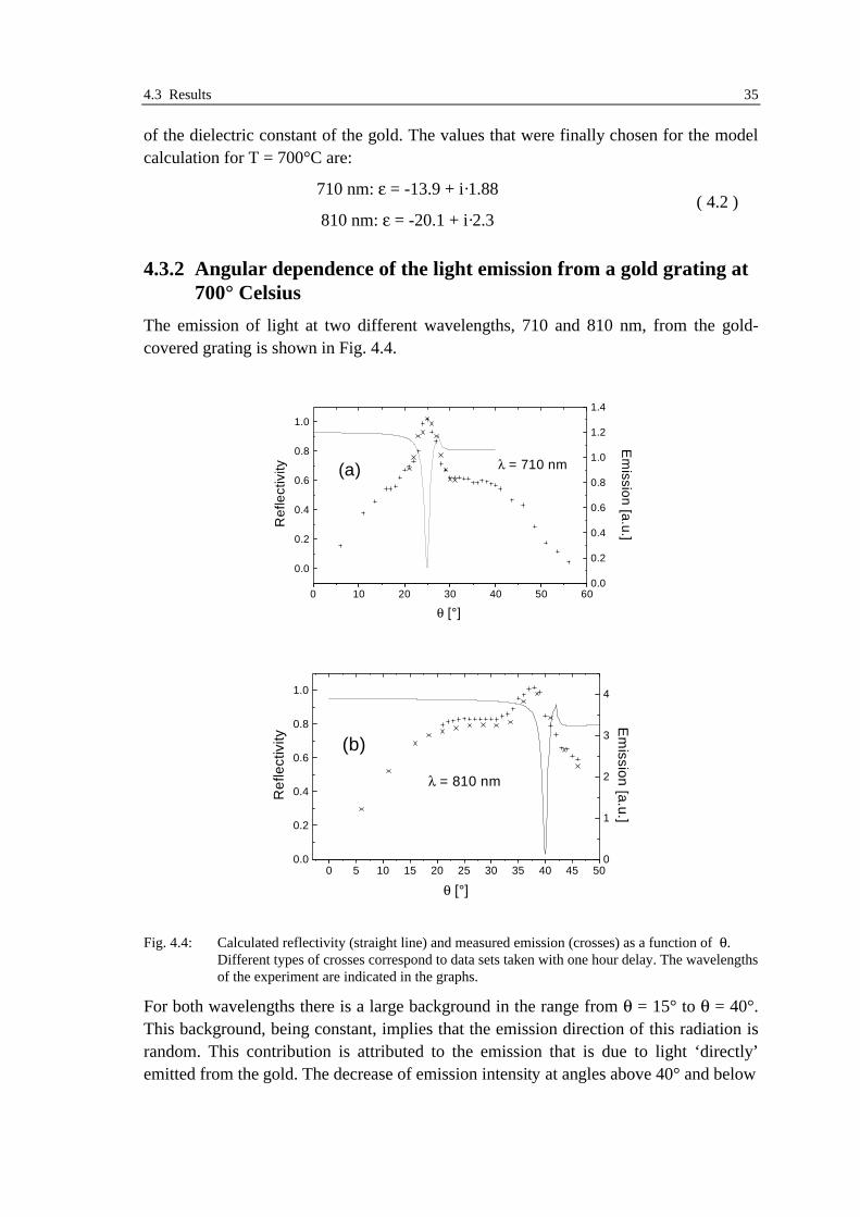
4.3 Results 35
of the dielectric constant of the gold. The values that were finally chosen for the modelcalculation for T = 700°C are:
710 nm: ε = -13.9 + i·1.88
810 nm: ε = -20.1 + i·2.3( 4.2 )
4.3.2 Angular dependence of the light emission from a gold grating at700° Celsius
The emission of light at two different wavelengths, 710 and 810 nm, from the gold-covered grating is shown in Fig. 4.4.
0 10 20 30 40 50 60
0.0
0.2
0.4
0.6
0.8
1.0
λ = 710 nm
Ref
lect
ivity
θ [°]
0.0
0.2
0.4
0.6
0.8
1.0
1.2
1.4
(a)
Em
ission [a.u.]
0 5 10 15 20 25 30 35 40 45 500.0
0.2
0.4
0.6
0.8
1.0
λ = 810 nm
Re
flect
ivity
θ [°]
0
1
2
3
4
(b)
Em
ission [a.u.]
Fig. 4.4: Calculated reflectivity (straight line) and measured emission (crosses) as a function of θ.Different types of crosses correspond to data sets taken with one hour delay. The wavelengthsof the experiment are indicated in the graphs.
For both wavelengths there is a large background in the range from θ = 15° to θ = 40°.This background, being constant, implies that the emission direction of this radiation israndom. This contribution is attributed to the emission that is due to light ‘directly’emitted from the gold. The decrease of emission intensity at angles above 40° and below

36 4 Thermally induced emission of light...
15° is an artefact due to imperfect experimental geometry. For both wavelengths, thereis a distinct emission peak visible, which can be attributed to surface-plasmon-enhancedemission. This is proven by comparing the observed emission peaks to calculatedreflectivities for the two wavelengths under investigation, which are plotted as straightlines.
Coupling of light to surface plasmons in a reflectivity experiment would occur in thesame angular range where the maximum in emission is observed. From this, it can beconcluded that indeed the coupling of thermally excited surface plasmons to light viathe grating is responsible for these emission maxima. The widths of the emission peakand the plasmon minimum differ significantly: the emissivity maxima appear to bemuch broader than the reflectivity minima. This can be attributed to the limitedresolution in wavelength and emission angle in the emission measurement, giving anexperimental resolution of about 3 degrees. This effect is responsible for the relativelysmall height of the emission maximum, too. At a wavelength of 810 nm it seems thatthe emissivity maximum is slightly shifted with respect to the reflectivity minimum.This can be regarded as an artefact which is due to imperfect imaging of the grating ontothe photodetector.
4.3.3 Polarisation of the plasmon enhanced emission
In reflectivity measurements, only TM-polarised light couples to surface plasmons in theclassical mount. Thus, the radiation due to thermally excited surface plasmons, coupledout by a diffraction grating, is expected to be TM-polarised.
15 20 25 30 35 40
0.25
0.30
0.35
0.40
0.45
0.50
0.55
0.60
TM TE
Em
itte
d In
tens
ity [
a.u.
]
θ [°]
Fig. 4.5: Intensities of the TM-polarised and the TE-polarised component of the emitted light forλ = 710 nm as a function of the polar angle θ of the emission.
The above predicted behaviour was found for the maxima in the emission as it can beseen in Fig. 4.5 for λ = 710 nm where the separately recorded TM- and TE-component

4.4 Conclusion 37
of the emitted radiation are shown. The radiation background which contributed to bothpolarisations in roughly the same strength does not show a specific polarisationbehaviour while the peak due to surface plasmon enhanced emission is purely TMpolarised.
4.4 Conclusion
The emission of light in the visible/NIR from an optical gold grating at 700°C wasinvestigated with respect to it’s propagation direction and polarisation. For wavelengthsof 710 and 810 nm, there is a maximum observed in the emission-angle scan that ispurely TM-polarised. From the polarisation behaviour and the analysis of the directionof the emission, these maxima are attributed to thermally excited surface plasmonscoupled to light by the grating.
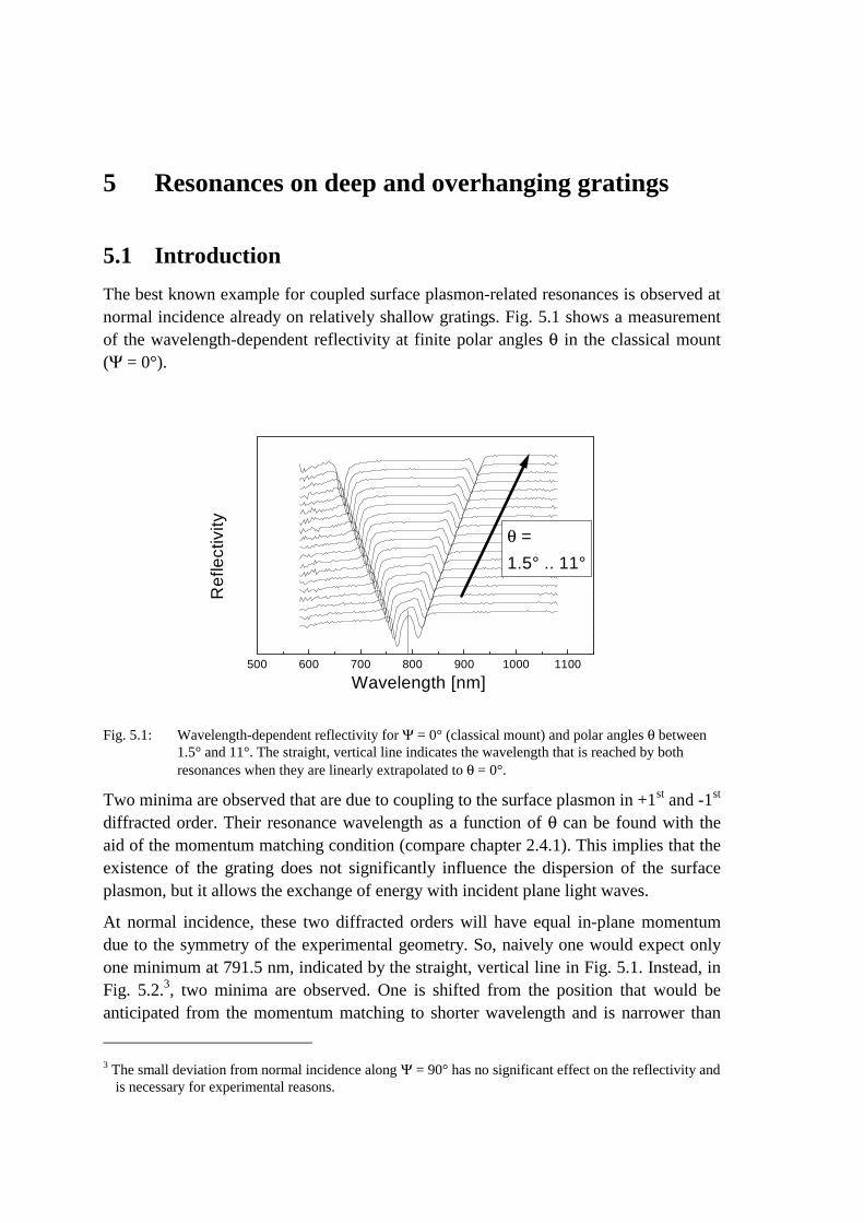
5 Resonances on deep and overhanging gratings
5.1 Introduction
The best known example for coupled surface plasmon-related resonances is observed atnormal incidence already on relatively shallow gratings. Fig. 5.1 shows a measurementof the wavelength-dependent reflectivity at finite polar angles θ in the classical mount(Ψ = 0°).
500 600 700 800 900 1000 1100
θ =
1.5° .. 11°
Ref
lect
ivity
Wavelength [nm]
Fig. 5.1: Wavelength-dependent reflectivity for Ψ = 0° (classical mount) and polar angles θ between1.5° and 11°. The straight, vertical line indicates the wavelength that is reached by bothresonances when they are linearly extrapolated to θ = 0°.
Two minima are observed that are due to coupling to the surface plasmon in +1st and -1st
diffracted order. Their resonance wavelength as a function of θ can be found with theaid of the momentum matching condition (compare chapter 2.4.1). This implies that theexistence of the grating does not significantly influence the dispersion of the surfaceplasmon, but it allows the exchange of energy with incident plane light waves.
At normal incidence, these two diffracted orders will have equal in-plane momentumdue to the symmetry of the experimental geometry. So, naively one would expect onlyone minimum at 791.5 nm, indicated by the straight, vertical line in Fig. 5.1. Instead, inFig. 5.2.3, two minima are observed. One is shifted from the position that would beanticipated from the momentum matching to shorter wavelength and is narrower than
3 The small deviation from normal incidence along Ψ = 90° has no significant effect on the reflectivity and
is necessary for experimental reasons.

5.2 Classification of resonances in model calculations 39
the ‘ordinary’ surface plasmon resonance. The other one appears at a longer wavelengthand shows a broadening. In analogy to the band gaps of electronic and vibrational statesat the Brillouin zone edge of a solid, this splitting is referred to as a ‘Photonic band gap’[Bar96].
740 760 780 800 820 840 8600.0
0.2
0.4
0.6
0.8
1.0
Λ = 773.6 nm
A1 = 19.8 nm ϕ
1 = 0°
A2 = 6 nm ϕ
2 = 40.3°
A3 = 3 nm ϕ
3 = 46°
Ref
lect
ivity
Wavelength [nm]
Fig. 5.2: Wavelength-dependent reflectivity for Ψ = 90° and θ = 1.5°, The measured values (dots) arecompared to a model calculation (straight line) based on a grating profile which is describedby the parameters shown in the inset The dielectric function is assumed as Drude-like withωp = 1.2 × 10¹⁶s−1 and τ = 7 × 10⁻¹⁵s. The position where a resonance would be expectedfrom the momentum matching approach is indicated by a vertical line (λ = 791.5 nm).
Here, the effect of the grating cannot be reduced to a channel that allows the coupling oflight to a surface plasmon resonance which propagates then along the grating like on aplane surface. Instead, there is an additional effect of the surface geometry on theresonances themselves. In order to distinguish these electromagnetic waves from thesurface plasmons which behave like 2-dimensional light, they are called ‘coupledresonances’ in this work.
The effect of an increased perturbation of the surface plasmon resonance, due to anincreased depth of the grating grooves is explored in this chapter for deep andoverhanging gratings. In the next section (5.2), a classification of the expectedresonance phenomena is presented, based on model calculations. The theoreticalpredictions are compared with measurements in chapter 5.3.
5.2 Classification of resonances in model calculations
This section attempts to bring some order to the big variety of resonances on deepdiffraction gratings. The already well studied ‘photonic band gap’ on shallow gratings isshortly reviewed and a new interpretation, that highlights the symmetry of theelectromagnetic problem is given. Then, the reflectivity of deep gratings is studied. The

40 5 Resonances on deep and overhanging gratings
properties of deep, symmetric gratings are re-interpreted with special emphasis on theirsymmetry. This will allow some understanding of the features that are found on slightlyasymmetric gratings that have, to my knowledge, not been reported in literature. A shortlook at extremely asymmetric gratings will complete this overview. But first, somegeneral remarks have to be made about the reflection geometry and a definition must begiven what is meant by ‘symmetry’ of a grating in the further considerations.
5.2.1 Reflection geometry
The model calculations that are presented below are all referring to light that falls on thegrating structure along the surface normal (θ = 0°). The electrical field vector isperpendicular to the grating grooves (Ψ = 0°, ϕ = 0°). The dielectric constant of themetal is assumed to have a Drude-type behaviour (see Chapter 2.2) with a plasmafrequency of ωp = 1.2 × 10¹⁶s−1 and a collision time of τ = 7 × 10⁻¹⁵s. These parametersare chosen to give dielectric constants similar to gold.
5.2.2 Symmetries in the grating profile
The profile of the gratings under investigation is modelled as a Fourier sum
( )z x A i xi ii
= ⋅ ⋅°
⋅ +
=
∞
∑ sin360
1 Λϕ ( 5.1 )
Where z and x denote the Cartesian co-ordinates of the profile, Ai are the amplitudesand ϕi the phases of the i’th harmonic. The phase of the first Fourier component ischosen to be ϕ1 = 0°. Λ is the grating pitch which should be in the range of thewavelength of the electromagnetic radiation that is to be diffracted. In all the followingcalculations, Λ = 700 nm is assumed because the experimental results in the nextchapter will be on gratings with roughly this pitch.
(a) ϕ2 = 90° (b) ϕ2 = 270° (c) ϕ2 = 0°
Fig. 5.3: Grating profiles formed of a fundamental of unit amplitude A1 = 1 and a second harmonicwith an amplitude of A2 = ¼, and different choices for the phase of the second harmonic ϕ2.Below the resulting profile, the 2nd harmonic is shown. For the two possible choices withmirror symmetry, the mirror planes are indicated as lines.
The investigation of a profile that is composed of only two components already yieldsimportant insights to the physical processes and symmetry properties involved in thecoupling of light to surface plasmon related resonances. Fig. 5.3 shows three selected

5.2 Classification of resonances in model calculations 41
grating profiles that can be constructed by choosing different ϕ2. The ratio of the firsttwo amplitudes, A1/A2 is chosen to be 4. It is important to note that there are only 2possible choices for ϕ2 that lead to a profile with mirror symmetry with respect to themirror planes that are indicated in the graph, namely ϕ2 = 90° which leads to a ‘broadpeak profile’ and ϕ2 = 270° describing a ‘broad trough profile’.
With all other choices for ϕ2, asymmetric profiles are obtained as, for example in Fig.5.3 (c), where ϕ2 = 0°. Such asymmetric gratings are called ‘blazed gratings’ (e. g.[Tam77]) . The higher Fourier components can be treated in a similar way. There areonly two choices for the phase of the higher harmonic components that preserve themirror symmetry.
There are two reasons why this mirror symmetry is important. Firstly, in many cases,there is no asymmetry in the grating preparation process so that 90°/270° are the onlypossible values ϕ2 may take. Secondly, the symmetry of the profile has a stronginfluence on the resonances that are supported by the grating, as will be shown in thenext section.
5.2.3 Shallow gratings
The resonances at the ‘photonic band gap’ on shallow4 gratings at normal incidencehave been intensely investigated [Kit95b], [Fis95], [Bar95]. For a comprehensive anddetailed treatment of the subject the reader is referred to the excellent review article byBarnes et. al. [Bar96]. Here, only the aspects that are essential for the following arepresented.
When the coupling condition for the surface plasmon is fulfilled at normal incidence,this is the case simultaneously for the 1st and -1st order. Furthermore, the secondharmonic component of the grating profile provides the momentum that is required forcoupling between these two energetically degenerate states. As a consequence, they splitinto a high energy and a low energy coupled state.
In Fig. 5.4, reflectivities for different grating shapes are shown. The profiles are the onesthat were already shown in Fig. 5.3: either the fundamental Fourier component only,(pure sine function) or the fundamental and a second harmonic.
In the absence of a second harmonic component (A2 = 0 nm), the surface plasmonposition is exactly where it is expected from the momentum-matching approach (λ =720 nm). For such a grating, there is an unperturbed crossing between the surfaceplasmons coupled in +1st and -1st order. For the asymmetric grating (A2 = 5 nm, ϕ2 = 0),two resonances are clearly seen, one is shifted to smaller wavelengths relative to theoriginal resonance and has become narrower, the other one has shifted to longerwavelengths and has become broader. Since for optical resonances, broad features
4 The total vertical peak-to-trough distance is much smaller than Λ.

42 5 Resonances on deep and overhanging gratings
correspond to a short propagation (or rather coherence- ) length, the terms ‘Long rangesurface plasmon’ (LRSP) for the narrow and ‘Short range surface plasmon’ (SRSP) forthe broad resonance were chosen for this work5. From this observation, the conclusioncan be drawn that the second harmonic component of the grating profile plays animportant role in the formation of coupled resonances.
The two symmetric gratings support only one resonance each. The resonancewavelength on the ‘broad peak’ profile (A2 = 5 nm, ϕ2 = 90°) is identical to the SRSPwhereas the resonance wavelength on the ‘broad trough’ profile (A2 = 5 nm, ϕ2 = 270°)is the one of the LRSP.
660 680 700 720 740 760 780 800 820
A2 = 5 nm
ϕ2 = 0°
A2 = 5 nm
ϕ2 = 270°
A2 = 0 nm
A2 = 5 nm
ϕ2 = +90°
Re
flect
ivity
Wavelength [nm]
Fig. 5.4: Reflectivity for different wavelengths for a grating with a pitch of Λ = 700 nm and a profilewith a first Fourier component A1 = 20 nm and A2 as indicated.
For the deeper understanding of the nature of these surface resonances, it is helpful toanalyse their electromagnetic field distribution. Fig. 5.5 shows the magnetic fielddistributions for the one coupled resonance each which is observed on a purelysinusoidal, on a ‘broad peak’ and on a ‘broad valley’ grating. For the blazed grating,field distributions corresponding to the two resonances that are visible in Fig. 5.5 areshown.
For geometrical reasons, only the y-component of the magnetic field (The one parallel tothe grating grooves) does not vanish, therefore the magnetic field can be represented asa (complex) scalar function. In all field distributions, the modulus of this function isplotted.
5 The same terms are used in the case of surface plasmon coupling between two identical surfaces of a
very thin metal film. In this case, too, there are two coupled resonances formed with different widths[Sar76].

5.2 Classification of resonances in model calculations 43
(a) A2 = 0 λ = 720 nm (b) ϕ2 = 90° λ = 727 nm (c) ϕ2 = 270° λ = 712 nm
Normal surface plasmon SRSP LRSP
1 µm
(d) ϕ2 = 0° λ = 712 nm (e) ϕ2 = 0° λ = 727 nm
LRSP SRSP
Fig. 5.5: Modulus of the magnetic field for grating profiles as introduced in Fig. 5.3. The phase of thesecond harmonic and the wavelength of the incident light are indicated below the pictures.White corresponds to the maximum value, black to 0. Above the pictures, the surface profileand the second harmonic are sketched with an exaggerated amplitude. The scale correspondsto the field distributions.
Strong modulation of the magnetic field along the interface is observed with twointensity maxima per fundamental oscillation of the grating profile. The positions ofthese maxima depend on the surface profile. For the pure sine (a), the ‘broad peak’ case(b) and the ‘broad valley’ case (c) they are located in the valleys and on the tops of thefundamental component. Nodes are observed in the slopes of the surface profile. Thetwo resonances on the blazed gratings have similar field distributions but the fieldmaxima are shifted by roughly 1/8 of the fundamental. The LRSP is characterised by ato the left (d) whereas the SRSP is shifted to the right (e).
In the next step, two questions will be addressed: what is responsible for the shift inresonance wavelength of the coupled resonances and why are they partly missing forsymmetric gratings?
5.2.3.1 The role of the second harmonic of the grating profile
It has been already mentioned that the second component of the Fourier representationof the grating profile is responsible for the mutual coupling between the two ‘free’plasmons and the formation of the band gap. It turns out that the direction of the shift inwavelength of a coupled resonance depends on the position of the magnetic fieldmaxima relative to the second harmonic of the grating profile. The SRSP has itsmagnetic field maxima in the minima of the second harmonic whereas the LRSP’smagnetic field is concentrated on the maxima of the second harmonic. For the detaileddiscussion of the underlying physics, the reader is referred to the paper of Barnes et al.[Bar96]. Now, by comparison of the magnetic field distributions (Fig. 5.5) with therelative position of first and second harmonic (as drawn in Fig. 5.3), the shifts in

44 5 Resonances on deep and overhanging gratings
wavelength that are observed in Fig. 5.4 can be understood. Magnetic fields in themaxima of the second harmonic lead to a LRSP at λ = 712 nm. A SRSP (λ = 727 nm) ischaracterised by magnetic fields in the minima of the second harmonic. Without asecond harmonic, there is no shift.
5.2.3.2 ‘Selection rules’
Another important question is why for symmetric gratings there is always one of theresonances missing. In the paper of Barnes et. al. this is explained by considering thecomponent of the incident electrical field normal to the metal surface which is needed toproduce a surface charge6. Coupling is possible only to the surface modes with a chargedistribution that is in phase with the one produced by a non-vanishing component of theexciting electrical field normal to the metal-dielectric interface. An analysis of thecharge distribution that would be needed to set up resonances with maxima in the peaksor troughs of the second harmonic of the grating profile, it turns out that on symmetricgratings there is always one in phase with the exciting charge distribution while theother one is phase shifted by 90°. As a consequence, the one is maximally coupled andthe other one is not observed. With the same reasoning, it can be explained why there iscoupling to both resonances for the blazed grating: here, we twice deal with a phaseshift of exciting charge distribution and resonance intrinsic charge distribution of 45°.
I wish to present a slightly different approach to the problem, which seems to be moreintuitive. The underlying physics is, of course, the same. It is based on considerations ofthe symmetry of the grating and the exciting field. We start again by examining theresponse of the two symmetric gratings in the example given above. The ‘missing’resonances would have nodes of the magnetic field intensity on the peaks and in thetroughs of the fundamental in order to have the correct position relative to the secondharmonic of the grating profile. Why are they not coupled to?
In order to answer this question, we need to recall that the mathematical problem ofreflection of a monochromatic electromagnetic wave on any dielectric configuration canbe either described by the electrical or magnetic field. Both give the full description ofthe solution and if one is given, the other one is easily calculated by using Maxwell’sequations. In the case that is considered here, the easier choice is the magnetic fieldsince it has only one non-vanishing component, Hy.
Now, consider the symmetry of the entire system. The geometry is specified by thepropagation direction and polarisation of the incident magnetic field and the surfaceprofile. Obviously, all the physical quantities and therefore the full problem have mirrorsymmetry with respect to the mirror planes as indicated in Fig. 5.3. An allowed solutionmust exhibit the same symmetry. In Fig. 5.5, the modulus of the magnetic field of the
6 Please note that the assumption that only the normal component is responsible for the excitation should
be doubted, compare chapter 7. Nevertheless, the analysis of Barnes et al. is still valid with minoradaptations.

5.2 Classification of resonances in model calculations 45
allowed solution is plotted, and the predicted symmetry is observed in this example.But, since the time dependent magnetic field is given by a complex function, we have toconsider the phase as well. When a node in the magnetic field distribution is observed,there is always a phase jump by 180° associated with it (because the first derivative ofthe magnetic field must be continuos ).
0 200 400 600 800 1000
100
150
200
250
Ph
ase
[°]
x [nm]
Fig. 5.6: Phase of the magnetic field 200 nm above the surface for the resonance on the ‘broad valley’profile (see Fig. 5.5 c). Above, the surface profile is sketched together with its secondharmonic component, the vertical line indicates the common mirror plane of surface profileand field distribution.
This is illustrated in Fig. 5.6 for a ‘broad valley’ mirror symmetric grating. Comparisonwith (Fig. 5.5, c) shows that indeed a phase jump of 180° is observed at each node of themagnetic field. Furthermore, the right symmetry of the phase (Fig. 5.6) and the modulusvalue of the magnetic field is seen for this example.
Now, it is obvious, why there is no SRSP for the ‘broad valley’ grating. Such a mode,having its magnetic field maxima in the troughs of the 2nd harmonic of the gratingprofile would have a node right in the mirror plane. The associated phase jump wouldbreak the mirror symmetry and a solution with odd symmetry (symmetric modulus butreversed sign upon reflection) would be obtained instead.
It is instructive to do the same analysis for the electrical field. Here, things are a littlemore complicated because there are two components of the electrical field that have tobe considered, z and x direction. The absolute values of these field components areplotted in Fig. 5.7. For each component there is again a phase jump of 180° at eachnodal plane for the same reasons as discussed above.

46 5 Resonances on deep and overhanging gratings
400
nm
Ex
Ez
Fig. 5.7: Electrical field distribution for LRSP of the ‘broad valley’ profile. The absolute value of thex and z component are plotted as grey values. White indicates the maximum value, black 0.
The calculated x component has odd symmetry with respect to the mirror plane. Thisbehaviour is expected, because the incident electrical field is polarised in x direction.Upon inversion on the mirror plane, this field reverses its sign. Therefore, the initialproblem has odd symmetry.
The calculated z component has even symmetry with respect to the mirror plane. This,again, reflects the symmetry of the system: like a vector in y-direction (as the magneticfield in the example considered above), a vector in z-direction keeps its orientation uponreflection.
As soon as the grating looses mirror symmetry, there are no restrictions to the symmetryof the electromagnetic field distributions. That is why both resonances are coupled toincident light on a blazed grating.
5.2.4 Deep gratings with mirror symmetry
Now, after having got some insight into the coupled resonances in the relatively simplecase of a shallow grating, the focus now is on the additional effects that come into playwhen the grating amplitude is increased. It is most instructive to vary both thewavelength of the incident light and the grating amplitude continuously and investigatethe dispersion of the resonances which can be observed as areas of reduced reflectivityin the plane which is spanned by these two parameters. The grating amplitude is alwaysvaried by applying a linear scaling factor sc to all Fourier components of one gratingprofile, thus keeping the ratios between the individual amplitudes fixed.
( ) ( )z x sc z x sc A i xscaled i ii
= ⋅ = ⋅ ⋅ ⋅°
⋅ +
=
∞
∑ sin360
1 Λϕ ( 5.2 )
Since sc is not a very intuitive quantity, the resulting fundamental amplitude sc. A1 isused as a measure of the total grating amplitude. In Fig. 5.8, the reflectivity of a deep‘broad peak’ grating is plotted as grey values when the wavelength of the incident lightand the grating amplitude are varied.

5.2 Classification of resonances in model calculations 47
800 1000 1200 1400 16000
100
200
300
400
500
600
700
b
c
a
d
Wavelength [nm]
A1
[nm
]
A1 = 350 nm
A1 = 700 nm
Fig. 5.8: Calculated reflectivity map of a grating (Λ = 700 nm) of the form as shown on the right as afunction of grating amplitude and wavelength of the incident light. The grey values indicatedifferent reflectivities from 0.5 (black) to 1 (white). The arrows indicate where fielddistributions will be calculated. The maximum grating profile has the Fourier componentsA1 = 700 nm, A2 = 175 nm, ϕ2 = 90°.
The pseudocritical edge at λ = 700 nm where the first diffracted orders becomeevanescent is clearly seen as a sharp rise in intensity. For longer wavelengths, thegrating is of zero order, that means that all diffracted orders are evanescent. In thisregion, four extended dark stripes, indicating low reflectivity, are observed. Theseresonances move to the infrared for increasing grating amplitudes.
1 µm
(a) λ = 750 nm (b) λ = 757 nm (c) λ = 750 nm (d) λ = 1595 nm
A1 = 52.5 nm A1 = 245 nm A1 = 648 nm A1 = 578 nm
Fig. 5.9: Spatial distribution of the magnetic field strength as grey values (white indicating highmagnetic field strength) for some selected resonances in the reflectivity map (Fig. 5.8). Thescaling bar applies to all images.

48 5 Resonances on deep and overhanging gratings
An analysis of the magnetic field distribution across the grating structure in theseresonances, shown in Fig. 5.9, gives some insight into the nature of these features.
The distributions (a, b, c) are taken at about the same wavelength for increasingamplitude of the grating as indicated in Fig. 5.8. They correspond to the first, secondand forth ‘branch’. It can be seen that each branch has a unique topology of the magneticfield distribution, with a characteristic number of nodal planes and maxima. For each‘step upwards’, one nodal plane, spanning the grating groove, is added. Fig. 5.9 (d) lieson the same branch as (b) which is reflected in the same number of maxima and nodesof the magnetic field inside the groove. In the following, these higher resonances will becalled MEi (‘magnetic even’) where the integer i denotes the number of separated fieldmaxima inside the grating groove.
If we recall the symmetry constraints to an allowed solution of the electromagneticboundary problem, it is seen that these ‘ladders’ have the required even symmetry. Itshould be noted that they are not the only possible solutions. Lopez-Rios [Lop98] hasinvestigated a shallow grating with very widely separated grooves where additionalnodes show up on top of the grating peaks. Additionally, closed loops of nodal planesinside the grating grooves cannot be excluded by symmetry considerations.
It should be mentioned that predictions for this type of resonances on deep diffractiongrating can be found in literature. The first of these resonances is identical to the SRSPin the limit of very small grating amplitudes. For higher amplitudes, the field gets moreconcentrated inside the groove at the expense of the field strength on the top of thegrating. This resonance has been described by various authors [Gar96], [Lak81].
The whole family of resonances that is found on deeper gratings was described by Wattset al. [Wat97] and Sobnack at al. [Sob98], the latter giving a good intuitiveinterpretation. The electromagnetic surface modes propagate along the grating tops assurface plasmons while they have to be described as waveguide modes inside thegroove. The total phase that is picked up by such a mode between two equivalent pointson the grating must equal a multiple integer of 2π. An approximate analyticalcalculation based on this model leads to a good agreement compared to the rigorousmodelling. Maradudin et al. [Mar97] considered a single groove in an otherwise planemetal surface and found similar resonances.
Currently there is much interest in the transmission through slits in metal layers whichare of the order of the wavelength of light or smaller as recent theoretical papers show[Ast00], [Por99]. A strong enhancement of the transmission due to excitation oflocalised resonances inside the grooves is predicted. Experimental results on 2-dimensional arrays of holes are presented by Ebbesen [Ebb98], in this work, nolocalised resonances inside the holes were found because of the small thickness of themetal film.

5.2 Classification of resonances in model calculations 49
A purely sinusoidal grating shows almost no resonance features for increasing depths(not shown). The conclusion must be drawn that the reflectivity of a deep grating is verysensitive to its shape.
5.2.5 Deep, asymmetric gratings
From the investigations on shallow gratings it can be already assumed that a brokensymmetry will make the optical response of deep gratings richer. Some theoreticalinvestigations on this problem are presented in a paper by Preist et al. [Pre97]. Wanstallet al. [Wan98] concentrate on highly overhanging gratings and find a family ofresonances similar to the ladder of the MEi resonances that was discussed above. Still,there is no investigation on slightly blazed, deep gratings in the literature. For thisreason, the additional features that are introduced by the asymmetry of the grating andtheir evolution when the asymmetry is increased are presented in this subsection.
5.2.6 A ‘new’ resonance
The asymmetry is introduced to the grating shape by applying the obliquetransformation which is given by the obliquity angle θob (See chapter 2) to the pointsthat describe the grating profile
Already a very small blaze (θob = 87°) has got a drastic effect on the resonance structureas it can be seen in Fig. 5.10.
600 800 1000 1200 1400 1600 18000
50
100
150
200
250
300
350
b
c
a
Wavelength [nm]
A1
[nm
]
A1 = 190 nm
A1 = 380 nm
Fig. 5.10: Calculated reflectivity map of a grating of the form as shown on the right as a function ofgrating amplitude and wavelength of the incident light. The grey values indicate differentreflectivities from 0.5 (black) to 1 (white). The arrows indicate for which parameters fielddistributions will be calculated. The maximum grating profile has the Fourier componentsA1 = 380 nm, A2 = 10.6 nm, ϕ2 = 26.3°, A3 = 23.4 nm, ϕ3 = 36.3°, the oblique angle equalsθob = 87°.

50 5 Resonances on deep and overhanging gratings
The first two MEi resonances are visible in this plot only very weakly due to the smalldeviation of the profile from the pure sine. Additionally, a very deep and narrowresonance appears which had not been observed for mirror symmetric gratings. In thelimit of a shallow grating this new feature is identical to the LRSP. A view on themagnetic field distributions (Fig. 5.11) reveals why this resonance appears only onblazed gratings. The magnetic field distributions show almost odd symmetry which isonly possible because the mirror symmetry of the grating is slightly broken.
(a) A1 = 38 nm, λ = 673 nm (b) A1 = 152 nm, λ = 703 nm (c) A1 = 304 nm, λ = 757 nm
Fig. 5.11: Spatial distribution of the magnetic field strength as grey values (white indicating highmagnetic field strength) for some selected resonances in the reflectivity map (Fig. 5.10). Theimages are drawn to scale. The scale has been suppressed for better readability, each sectionis 1000 nm wide.
This finding allows an extension of the interpretation of the deep grating as array ofsmall waveguides as it was shortly reviewed above. It seems that these ‘waveguides’ areable to support two families of surface plasmon-related ‘lamellar’ resonances. The onefamily (MEi) is characterised by a magnetic field with even and an electrical field withodd symmetry. On shallow ‘broad peak’ gratings, this family is represented by theSRSP. The other family has an magnetic field with odd and an electric field with evensymmetry. It is not coupled to free electromagnetic radiation normally incident on amirror symmetric grating. Breaking of the symmetry of the grating profile allowscoupling and in consequence its observation.
An alternative way to excite modes with a magnetic field distribution with oddsymmetry is described by Watts et al. [Wat97]. They report the observation of aresonance that is coupled with TM light in a geometry where the plane of incidence isparallel to the grating grooves (Ψ = 90°) and the polar angle (θ) is different from 0°.There, additionally the existence of higher orders of this family of resonances for verydeep gratings has been shown in a model calculation. This experimental geometrypreserves the symmetry of the grating but offers an exciting magnetic field with oddsymmetry. The electrical field has even symmetry now. In some sense, the roles ofelectrical and magnetic field are exchanged compared to the MEi resonances. Fromthese considerations, these resonances are identified with the ones that are observed onslightly asymmetric gratings. In the further investigations these resonances will be called‘magnetic odd’ MOi.
It should be noted that due to the slightly broken symmetry of the grating profile, theeven or odd symmetry of these modes is not exact. But if the grating asymmetry is not

5.2 Classification of resonances in model calculations 51
too big, these labels are still helpful to understand the observed resonance patterns andare used in this and the following section.
5.2.6.1 Interaction between the two families of resonances
When the appropriate grating profile is chosen, the two families of resonances with evenand odd symmetry may appear in significant strength simultaneously. This makes thereflectivity map of such a grating relatively complex. Fig. 5.12 shows calculatedreflectivities for a ‘broad peak’ profile which is tilted by an obliquity angle of θob = 70°.The first 3 resonances with magnetic field with even symmetry (ME1, ME2, ME3) areseen as broad areas of slightly reduced reflectivity which move quickly to the infraredfor increasing grating amplitude.
800 1000 1200 14000
100
200
300
400
500
600
MO1
cp
ME3
ME2
ME2
ME3
MO1
ME1
MO1
Wavelength [nm]
A1
[nm
]
A1 = 300 nm
A1 = 600 nm
Fig. 5.12: Calculated reflectivity map of a grating of the form as shown on the right as a function ofgrating amplitude and wavelength of the incident light. The grey values indicate differentreflectivities from 0 (black) to 1 (white). The maximum grating profile has the Fouriercomponents A1 = 600 nm, A2 = 150 nm, ϕ2 = 90°. The oblique angle is θob = 70°. Theassignments on the arrows are explained in the text.
Close to the pseudocritical edge, a rich structure is seen that can be interpreted asfollows:
The areas of low reflectivity marked with an ‘MO1’ correspond to the first resonancewith a magnetic field of odd symmetry. The minima right at the pseudocritical edgebelong to the resonances with even-symmetric magnetic field again. That means: Acrossing of the MO1-resonance with the ME2 and ME3- resonances leads to thisreflectivity behaviour.
Of course, one must check that the assignment given above reflects the real physics. Themagnetic field distributions of the MO1 resonance and the ME2 resonance are shown inFig. 5.13 right before and after crossing each other. The ‘crossing point’ is indicated inFig. 5.12 as ‘cp’.
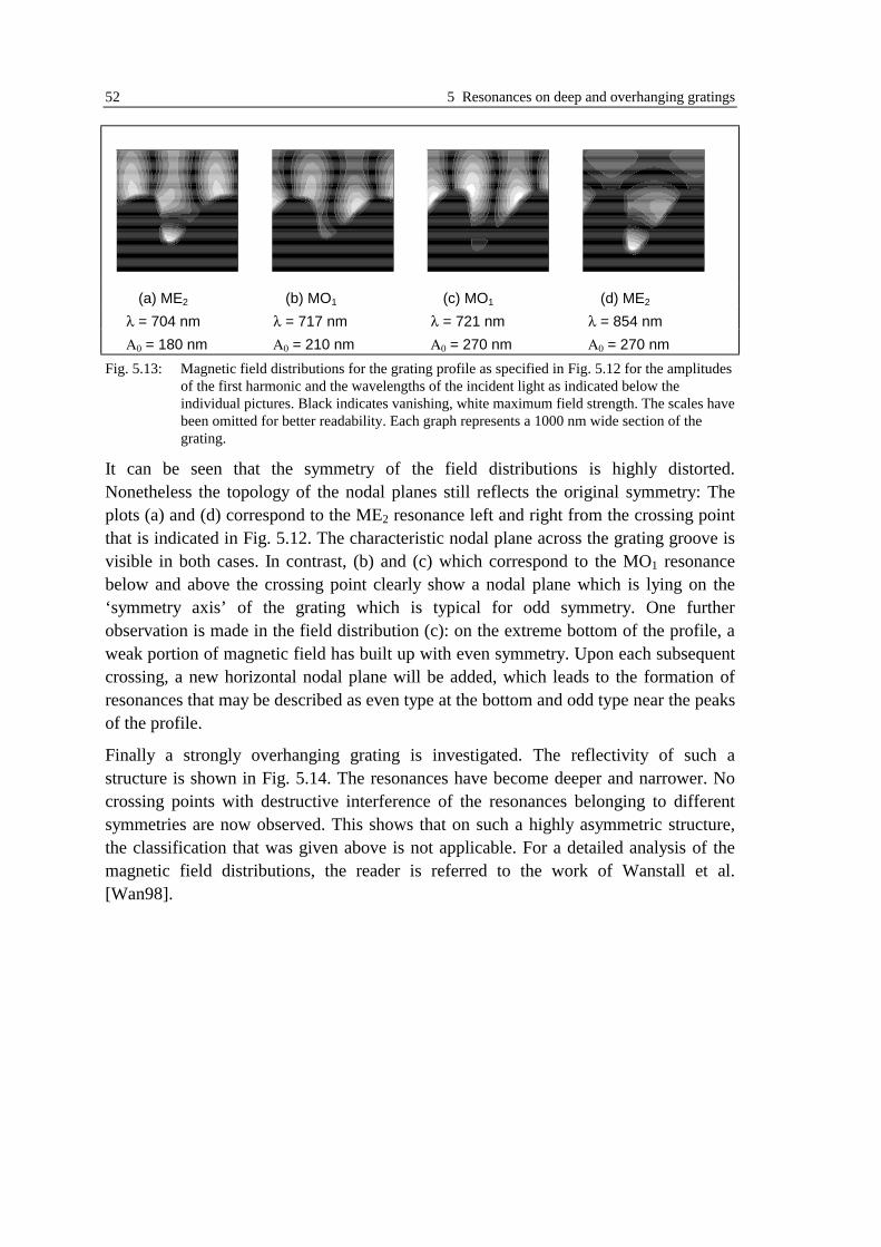
52 5 Resonances on deep and overhanging gratings
(a) ME2 (b) MO1 (c) MO1 (d) ME2
λ = 704 nm λ = 717 nm λ = 721 nm λ = 854 nm
Α0 = 180 nm Α0 = 210 nm Α0 = 270 nm Α0 = 270 nm
Fig. 5.13: Magnetic field distributions for the grating profile as specified in Fig. 5.12 for the amplitudesof the first harmonic and the wavelengths of the incident light as indicated below theindividual pictures. Black indicates vanishing, white maximum field strength. The scales havebeen omitted for better readability. Each graph represents a 1000 nm wide section of thegrating.
It can be seen that the symmetry of the field distributions is highly distorted.Nonetheless the topology of the nodal planes still reflects the original symmetry: Theplots (a) and (d) correspond to the ME2 resonance left and right from the crossing pointthat is indicated in Fig. 5.12. The characteristic nodal plane across the grating groove isvisible in both cases. In contrast, (b) and (c) which correspond to the MO1 resonancebelow and above the crossing point clearly show a nodal plane which is lying on the‘symmetry axis’ of the grating which is typical for odd symmetry. One furtherobservation is made in the field distribution (c): on the extreme bottom of the profile, aweak portion of magnetic field has built up with even symmetry. Upon each subsequentcrossing, a new horizontal nodal plane will be added, which leads to the formation ofresonances that may be described as even type at the bottom and odd type near the peaksof the profile.
Finally a strongly overhanging grating is investigated. The reflectivity of such astructure is shown in Fig. 5.14. The resonances have become deeper and narrower. Nocrossing points with destructive interference of the resonances belonging to differentsymmetries are now observed. This shows that on such a highly asymmetric structure,the classification that was given above is not applicable. For a detailed analysis of themagnetic field distributions, the reader is referred to the work of Wanstall et al.[Wan98].

5.2 Classification of resonances in model calculations 53
800 1000 1200 1400 16000
100
200
300
400
500
600
Wavelength [nm]
A1
[nm
]
A1 = 600 nm
A1 = 300 nm
Fig. 5.14: Calculated reflectivity map of a grating of the form as shown on the right as a function ofgrating amplitude and wavelength of the incident light. The grey values indicate differentreflectivities from 0 (black) to 1 (white). The maximum grating profile has the Fouriercomponents A1 = 600 nm, A2 = 150 nm, ϕ2 = 90°. The obliquity angle is θob = 20°.
5.2.7 Conclusion
The resonances that lead to absorption of light falling vertically on metallic gratingswere investigated in model calculations for a Drude-type metal. It was found that, onsymmetric gratings, two classes of resonances may exist with magnetic fielddistributions that exhibit either even or odd symmetry. At normal incidence, only theeven ones couple to light.
By introduction of a slight asymmetry to the grating profile, the resonances can still beroughly classified like in symmetric gratings. Now, both types are observed in the sameexperimental geometry and mutual interaction takes place. In the resonance pattern ofhighly asymmetric gratings the two classes are completely mixed.
An alternative way to couple to the resonances with odd symmetry of the magnetic fieldconsists in choosing an appropriate reflection geometry which differs from normalincidence. This observation was only shortly mentioned but will be explored to somemore detail later in this chapter.

54 5 Resonances on deep and overhanging gratings
5.3 Experimental results
In this section, reflectivity measurements on gratings with varying blaze and amplitudeare discussed and compared to model calculations. The depth and degree of asymmetrywas tuned by varying the geometry and exposure time in the etching process as isdescribed in chapter 3.
First (5.3.1), wavelength-dependent reflectivity data are presented that were taken at(almost) normal incidence on asymmetric gratings with the set-up that is described inchapter 3. For four different degrees of asymmetry, the measurements are compared tocompletely independently obtained theoretical calculations. Additionally, measurementsare shown for varying amplitude for these blazed gratings. In the following subsection(5.3.2), the theoretical prediction of stationarity of the red-shifted ME resonances isproved experimentally. Another subsection deals with measurements on a symmetricgrating where the experimental geometry is varied (5.3.3). Finally, (5.3.4) anexperimental observation that cannot be described with the idealised model of a perfectgrating is presented and an explanation is proposed.
5.3.1 Blazed gratings at ‘normal’ incidence
In this section, gratings, etched under different angles θetch = (10°, 20°, 30°, 40°), areinvestigated. See chapter 3 for details of the sample preparation and the opticalmeasurements. The experimental geometry is chosen to have the same symmetry asnormal incidence (polar angle θ = 4°, azimuthal angle Ψ = 90°) In this case, TE-polarisation has an electrical field perpendicular to the grating grooves. It is essentiallythe same as TM polarisation in the classical mount: The polarisation where coupling tothe surface plasmon resonance is possible. For each etching angle, the followingmeasurements and model calculations of the wavelength-dependent reflectivity arediscussed:
One sample is measured once and the surface profile obtained by electron microscopy.For this sample, the measured reflectivities are compared to theoretical predictions thatwere obtained on the basis of the grating profile as determined from the electronmicroscopy images. For these model calculations, the dielectric function of the gold wasmodelled as a Drude metal with plasma frequency ωp = 1.22 × 10¹⁶ s-1 and a collisiontime τ = 7 × 10-15 s. (compare chapter 2).
The effect of the variation of the grating amplitude on the surface resonances is studiedby recording the reflectivity spectrum after subsequent etching steps of another sample.It is intuitively clear that etching a pure gold grating will lead to a decreasing gratingamplitude. The precise grating shape after each individual step could not be measuredbecause the samples have to be broken to do so. For this reason, the profile that wasobtained from the first sample was used for model calculations of this experiment, too.These experimental data is compared to numerical data where a scaling factor between 0

5.3 Experimental results 55
and 2 is applied to the surface profile that allows observation of the amplitude-dependent dispersion of these resonances. It is neither known how much the gratingamplitude is decreasing by etching into the pure gold, nor if the originally determinedgrating profile is still applicable for strongly etched gratings. For this reason, aquantitative modelling of these experiments is not possible.
The interpretation of the data is delayed to the end of this subsection where acomparison of all experimental results is possible.
5.3.1.1 Etched at 10°
The measured and calculated reflectivity of a grating etched under 10° is shown in Fig.5.15 and Fig. 5.16 for illumination with TE and TM polarised light, respectively.Between λ = 1000 and 1100 nm the data sets taken with the two detectors overlap andform some ‘kinks’ which should not be regarded further. It is clearly seen that althoughthere is quantitative agreement between measurement and modelling, there are somediscrepancies with respect to the observed resonances.
The pseudocritical edge is observed at 650 nm in good agreement of theory andexperiment as expected. For short wavelengths, the measured reflectivity is much toolow while further in the infrared the measured values are approaching the theoreticalprediction for both polarisations.
For illumination with TE light, two resonances can be observed.
A very narrow and deep minimum appears around 700 nm which is predicted slightlytoo far in the infrared. This feature is assigned to the lowest resonance with magneticfield with odd symmetry (MO1)
7. The measured minimum appears broader andshallower than in the model calculation what is due to the finite wavelength resolutionof the set-up and the inhomogenity of the real grating.
The other resonance is much broader and further in the infrared. Again, there is adiscrepancy between theory and experiment with respect to its precise position.Additionally, this resonance appears deeper in the measurement than in the modelcalculation. It is assigned to the strongly red-shifted ME1 resonance.
The measurement with TM polarisation doesn’t show any resonance minimum inagreement with theory. This is the case for the other 3 degrees of blazing that will bediscussed later, too, for this reason these measurements with TM polarisation will not beshown.
7 In Fig. 5.10, exactly the same profile as here was used in a model calculation to introduce this kind of
resonance.

56 5 Resonances on deep and overhanging gratings
400 600 800 1000 1200 1400 1600 1800 2000
0.0
0.1
0.2
0.3
0.4
0.5
0.6
0.7
0.8
0.9
1.0
Measurement Calculation
718
690
1230
1090
Re
flect
ivity
Wavelength [nm]
Fig. 5.15: Measured (line with dots) and modelled (straight line) wavelength-dependent reflectivity ofthe sample etched at 10° for TE polarisation. The surface profile as determined from theSEM-image is shown in the graph. The arrows indicate the wavelengths of reflectivityminima that are attributed to surface resonances.
400 600 800 1000 1200 1400 1600 1800 20000.1
0.2
0.3
0.4
0.5
0.6
0.7
0.8
0.9
1.0
Measurement Calculation
Re
flect
ivity
Wavelength [nm]
Fig. 5.16: Measured (line with dots) and modelled (straight line) wavelength-dependent reflectivity ofthe sample etched at 10° for TM polarisation . The model calculation is based on the samesurface profile as for the TE case. (Fig. 5.15)
The measured dispersion of these two resonances as a function of the grating amplitudeare presented in Fig. 5.17 and the corresponding model calculation is shown in Fig.5.18. By comparison of the positions of the two resonances that are visible both intheory and experiment, the model calculations with scaling factors between 0.5 and 1are seen to correspond roughly to the measured data.

5.3 Experimental results 57
600 800 1000 1200 1400 1600 1800
increasing depth
Ref
lect
ivity
Wavelength [nm]
Fig. 5.17: Measured wavelength-dependent reflectivity of a gold grating etched under 10°. The deepestgrating was measured first and then the amplitude was decreased by subsequent etching steps.
400 600 800 1000 1200 1400 1600 1800 2000
sc = 0.1 .. 2
Ref
lect
ivity
Wavelength [nm]scaling = 0.5 .. 2
Λ = 650.8 nm
θob = 87°A1 = 189.4 nm ϕ1 = -104°
A2 = 5.3 nm ϕ
2 = 26.3
A3 = 11.7 nm ϕ
3 = 36.3 nm
Fig. 5.18: Modelled wavelength-dependent reflectivity for the grating shape that is produced by etchingunder 10° with scaling factors applied to the grating profile that vary between 0.1 and 2. Theparametrisation of the grating profile and sketches of the grating shape for some scalingfactors are shown on the right. The position of the ME1 is indicated by open circles. Thethicker line corresponds to the grating shape as determined by electron microscopy.
With respect to the dispersion of the MO1 resonance, the correspondence betweentheory and experiment is good. With increasing depth, this feature is slowly shifted intothe infrared. The strength of the resonance is not significantly altered for varyingamplitudes. The decreasing strength in the model calculation is observed for gratingamplitudes that were significantly higher than the measured ones (sc = 1.8). They werenot accessible to experimental investigations.

58 5 Resonances on deep and overhanging gratings
The influence of an increasing grating amplitude on the position and strength of the ME1
resonance is measured as predicted by the model calculation: A fast redshift isaccompanied by a significant weakening that makes the resonance difficult to see,especially in the model calculations. The absolute depth of this minimum is smaller inthe calculation than in the experiment.
5.3.1.2 Etched at 20°
The measured and modelled reflectivity of a grating etched under 20° is shown in Fig.5.19. Again, the measured reflectivity is significantly too low everywhere except at verylong wavelengths. The same resonances as in the previous section can be seen, still thereare only slight differences between theory and experiment.
The MO1 resonance is again measured at a shorter wavelength than predicted. Itsstrength has decreased with respect to the 10°-grating which is reflected both in theoryand experiment.
The position of the symmetric resonance is this time measured at a longer wavelengththan predicted. Furthermore, a slight increase in strength of this resonance can be seen.
400 600 800 1000 1200 1400 1600 1800 2000
0.0
0.1
0.2
0.3
0.4
0.5
0.6
0.7
0.8
0.9
1.0
Measurement Calculation
685
667
950
1040
Re
flect
ivity
Wavelength [nm]
Fig. 5.19: Wavelength-dependent reflectivity of the grating etched at θetch = 20° as determined from ameasurement compared to a model calculation. The surface profile as determined from theSEM-image is shown in the graph.

5.3 Experimental results 59
600 800 1000 1200 1400 1600 1800
increasing depth
Ref
lect
ivity
Wavelength [nm]
Fig. 5.20: Measured reflectivity as a function of wavelength of the incident light for a gold gratingetched under θetch = 20°. The deepest grating was measured first and then the amplitude wasdecreased by subsequent etching steps.
400 800 1200 1600 2000
scaling = 0.1 .. 2
Ref
lect
ivity
Wavelength [nm]
scaling = 0.5 .. 2
Λ = 659.5 nm
θob = 62.5°A1 = 149 nm ϕ1 = -97.5°
A2 = 11.2 nm ϕ2 = -78.6°
A3 = 2.5 nm ϕ
3 = 51.5°
Fig. 5.21: Modelled reflectivity for θetch = 20° as a function of wavelength for different gratingamplitudes. On the right, a graphical representation of the grating shapes and numericalvalues of the parameters are shown. The position of the very weak ME1 resonance isindicated by open circles. The thick line corresponds a grating shape as determined byelectron microscopy.
The measured dispersion as a function of the grating amplitude is presented in Fig. 5.20and the corresponding model calculation is shown in Fig. 5.21. Good agreementbetween theory and experiment was found regarding the changes that are due to theincreased asymmetry of the grating profile.
Little has changed with respect to the ME1 resonance compared to the grating etched at10° except a slight increase in strength.

60 5 Resonances on deep and overhanging gratings
The MO1 resonance shows a peculiar behaviour in the measurement. It shifts slightly tothe infrared and broadens. At the two deepest gratings, a new feature comes in from thepseudocritical edge while the MO1 has almost completely disappeared. Exactly thisbehaviour is seen in the model calculation. The model calculation of the region aroundthe pseudocritical edge is shown in an enlarged representation in Fig. 5.22.
600 800 1000
scaling =0.1 .. 2
Ref
lect
ivity
Wavelength [nm]
Fig. 5.22: Enlargement of Fig. 5.21
A comparison with the section 5.2.6.1 leads to the conclusion that this new minimum isdue to the second resonance with a magnetic field of even symmetry, ME2. From this, itcan be concluded that the maximum grating amplitude that could be produced liesslightly below the crossing point of the MO1 and the ME2 resonance. Because both themeasured wavelength of ME1 and the appearance of ME2 is expected for higheramplitudes, it can be assumed that the amplitude as it was determined from the electronmicrographs is too small. The model calculations with scaling factors between 0.7 and1.4 are tentatively assigned to the range of amplitudes that was experimentallyaccessible.
5.3.1.3 Etched at 30°
The measured and modelled reflectivity of a grating etched under 30° is shown in Fig.5.23. ME1 and MO1 can still be seen and the effect of the increasing asymmetry isconsistent in theory and experiment.
MO1 is again observed at a shorter wavelength than predicted. It has become shallowerthan in the previous examples.
ME1 is observed at a wavelength that is smaller than predicted. It has significantlygained in strength in the measurement. While the absolute strength is still significantlyunderestimated in the model calculations, an increase compared with the other modelcalculations can be observed.

5.3 Experimental results 61
400 600 800 1000 1200 1400 1600 1800 2000
0.0
0.1
0.2
0.3
0.4
0.5
0.6
0.7
0.8
0.9
1.0
Measurement Calculation
701
673
1211
1046
Re
flect
ivity
Wavelength [nm]
Fig. 5.23: Wavelength-dependent reflectivity of the grating etched at θetch = 30° as determined from ameasurement compared to a model calculation. The surface profile as determined from theSEM-image is shown in the graph.
400 800 1200 1600 2000
increasing depth
Ref
lect
ivity
Wavelength [nm]
Fig. 5.24: Measured wavelength-dependent reflectivity of a gold grating etched under 30°. The deepestgrating was measured first and then the amplitude was decreased by subsequent etching steps.

62 5 Resonances on deep and overhanging gratings
400 800 1200 1600 2000
scaling =0.1 .. 2
Ref
lect
ivity
Wavelength [nm] scaling = 0.5 .. 2
Λ = 636.6 nm
θob = 59°A1 = 196.7 nm ϕ1 = 105.9
A2 = 19.1 nm ϕ2 = 11.8
A3 = 8.6 nm ϕ3
= 14°
Fig. 5.25: Modelled reflectivity for θetch = 30° as a function of wavelength for different gratingamplitudes. The ME1 resonance is marked with open circles. The reflectivity correspondingto the grating amplitude as determined from the electron microscopy images is drawn as thickline. On the right, a graphical representation of the grating shapes and numerical values of theparameters are shown.
The measured dispersion of the resonances on this grating, as a function of the gratingamplitude is presented in Fig. 5.24 and the corresponding model calculation is shown inFig. 5.25. The MO1 resonance is relatively weak and weakens further with increasingamplitude, accompanied by a redshift. Similarly to the grating etched at 20°, for thehighest amplitude, this resonance has died out and the ME2 resonance comes in from thepseudocritical edge. This time, the appearance is predicted only for amplitudes that areslightly higher than measured. The measurements can be roughly assigned to the modelcalculations based on scaling factors between 0.5 and 1.1.
The ME1 resonance is still showing a redshift with increasing amplitude. Its strength hasincreased compared to the less blazed grating profiles that were discussed before but itis still much weaker in the model calculation than in the experiment.
5.3.1.4 Etched at 40°
The measured and modelled reflectivity of a grating etched under 40° is shown in Fig.5.26. There are still two resonances visible. But since the grating is already stronglyblazed, they cannot be labelled as MO/ME resonances although they seem to evolvesomehow from those.
This time, theory and experiment give the same wavelength where the short-wavelength-resonance is excited. A significant shift to shorter wavelengths of thisfeature is observed in comparison to the cases that were discussed above. The modelcalculation predicts that this resonance is expected to be very strong again. In the

5.3 Experimental results 63
measurement the strength is hard to estimate because of the finite resolution inwavelength.
The long wavelength resonance is again blue shifted in the measurement with respect tothe model calculation. It is stronger compared to all other profiles that were investigatedbefore. The absolute strength is underestimated in the model calculation.
400 600 800 1000 1200 1400 1600 1800 2000
0.0
0.1
0.2
0.3
0.4
0.5
0.6
0.7
0.8
0.9
1.0
Measurement Calculation
661
661
1220
1090
Re
flect
ivity
Wavelength [nm]
Fig. 5.26: Wavelength-dependent reflectivity of the grating etched at θetch = 40° as determined from ameasurement compared to a model calculation. The surface profile as determined from theSEM-image is shown in the graph.
400 800 1200 1600 2000
increasing depth
Ref
lect
ivity
Wavelength [nm]
Fig. 5.27: Measured reflectivity of a gold grating etched under 40°. The deepest grating was measuredfirst and then the amplitude was decreased by subsequent etching steps.

64 5 Resonances on deep and overhanging gratings
800 1200 1600
scaling =0.1 .. 2
Ref
lect
ivity
Wavelength [nm]
scaling = 0.5 .. 2
Λ = 648.7 nm
θob = 55°A1 = 197.2 nm ϕ1 = -137.8°
A2 = 38.9 nm ϕ2 = -71°
A3 = 1.7 nm ϕ3 = 135°
Fig. 5.28: Modelled reflectivity for θetch = 40° as a function of wavelength for differentgrating amplitudes. A weak resonance is marked by open circles where it is hard to see. Thethick line corresponds to the surface profile as determined from electron microscopy (scalingfactor of 1). On the right, a graphical representation of the grating shapes and numericalvalues of the parameters are shown.
The measured dispersion of the resonances on this grating, as a function of the gratingamplitude is presented in Fig. 5.27 and the corresponding model calculation is shown inFig. 5.28. In the measurement, the left resonance is first moving to shorter wavelengthswith increasing amplitude, and comes back then to longer wavelengths when the gratingamplitude is further increased. In the calculation, the resonance also first moves to theleft, but it disappears completely left from the pseudocritical angle. With furtherincreasing amplitude, a well pronounced resonance comes in again from shorterwavelengths, moving quickly to the infrared without disturbance. This suggests that thegrating is already blazed so strongly that the original description as resonances havingeven and odd symmetry with mutual perturbation at the crossing points is notappropriate any more. The observed behaviour resembles already the reflectivity that isfound for strongly overhanging structures (compare Fig. 5.14).
The long wavelength resonance may be identified with ME1. It is still showing a redshiftwith increasing amplitude. It appears stronger than in the previously investigated cases.This tendency is reflected in the model calculation, too, but the absolute intensity of thisresonance is predicted weaker than observed.
5.3.1.5 Overview on blazed gratings
The observations that were made regarding the impact of varying depth and asymmetryon the reflectivity of gold gratings are repeated here in a concentrated form to extract theimportant results. On the blazed gratings, three different types of resonances wereobserved for illumination by TE polarised light at Ψ = 90°, θ = 4°: two resonances witha magnetic field with even symmetry of the magnetic field, ME1 and ME2, and one withodd symmetry, MO1. In model calculations that are based on the independently

5.3 Experimental results 65
measured grating profiles, the essential features could be reproduced but there are someinconsistencies, too.
The first resonance with even magnetic field, ME1, is shifting to the infrared and getsweaker with increasing grating amplitude. This effect is well reflected in the modelcalculation. The difference between predicted and measured position could be accountedfor by applying a small scaling factor (ca. 0.9) to the grating profile in all cases exceptθetch = 20° (where the measured amplitude was too small). The strength of thisresonance increases with increasing blazing of the grating profile. This is well reflectedin the model calculations, while the theoretical prediction for the absolute depth of thisresonance is significantly smaller in all investigated cases.
The reflectivity minimum close to the pseudocritical edge can be addressed as the firstresonance with odd symmetry of the magnetic field (MO1) for the θetch = 10°, 20° and30°-gratings. It shows a slight redshift with increasing amplitude. This is theoreticallypredicted but its exact position is observed at smaller wavelengths in the measurementthan in the model calculation. This discrepancy cannot be overcome by a slight changeof the grating amplitude. Presumably, in this case it would be necessary to introduceeffects that are due to roughness of the grating. This resonance is fairly strong for theθetch = 10° grating and its strength decreases for increasing blaze. Additionally, thisresonance dies out for the deepest measured θetch = 20° and θetch = 30°-gratings. Both ofthe latter observations are made on the measurements as well as in the modelcalculations.
An additional reflectivity minimum is observed in the vicinity of the pseudocritical edgeon the deepest 20° and 30° gratings that could be fabricated. The agreement ofmeasurement and calculation regarding its strength and the grating amplitude of itsappearance is satisfactory. This allows the conclusion that this is the second resonancewith even symmetry of the magnetic field (ME2).
The correct prediction of the appearance of ME2 would require an increased amplitudefor the model calculation, whilst the correct position of MO1 requires a decreasing. Thisimplies that there are still refinements in the mathematical modelling to be developed.Presumably, the incorporation of sample roughness would give better results.Alternatively, the preparation of gratings with less roughness may give bettercorrespondence to theory.
The grating that was etched at 40° is already too strongly blazed for the resonances to bedescribed in terms of the even and odd symmetry. This is reflected in the fact that theshort wavelength minimum is fairly strong again, in contrast to the trend that wasobserved on the less strongly tilted gratings. Its position as a function of the gratingamplitude differs significantly from the latter behaviour, too. Instead of a red shift, a‘curve’, moving to the blue first and then coming back to the red is observed. All theseaspects are surprisingly well reproduced in the model calculation.

66 5 Resonances on deep and overhanging gratings
Independent of grating shape and polarisation there is much less light reflected thanpredicted by the model calculations, especially close to the pseudocritical edge. Thiseffect may be attributed to scattering on some random roughness of the samples.
No resonances are observed for TM polarised light. This indicates that the excitation ofthe observed minima requires a component of the electrical field normal to the metal /dielectric interface. This supports the interpretation of these resonances as self-interacting surface plasmons.
5.3.2 A stationary resonance
It was already pointed out by Wanstall et al. [Wan98] that the wavelength whereresonances are found on very deep and overhanging gratings does not change when the(polar) angle of incidence of the incoming beam is varied in the classical mount. This istotally different from the behaviour of ‘ordinary’ surface plasmons on shallowdiffraction gratings whose excitation wavelength obeys the momentum matchingcondition and is strongly angle-dependent (See Fig. 5.1). This theoretical prediction ischecked here on the sample that was etched under θetch = 40°. The wavelength-dependent reflectivity is shown for polar angles between 4° and 54° as determined frommeasurement and modelling in Fig. 5.29. For the calculation, a linear scaling factor ofsc = 0.95 was applied to the function representing the grating shape (compare Fig. 5.27)so that the minimum position for θ = 4° coincided with the one that was measured(λ = 1166 nm).
1000 1200 1400 1600 1800
(a)
Measurement
Ψ = 0°
θ = 4° .. 54°
Re
flect
ivity
Wavelength [nm]1000 1200 1400 1600 1800
(b)
Calculation
Ψ = 0°
θ = 4° .. 54°
Wavelength [nm]
Fig. 5.29: Measured (a) and modelled (b) wavelength-dependent reflectivity of the grating that wasetched at θetch = 40° as a function of wavelength. Different polar angles (θ) are chosen forΨ = 0° (classical mount).
A good agreement between model calculation and measurement is observed with respectto the resonance wavelength of the broad minimum, until (at θ = 54°) the pseudocriticaledge reaches the resonance and makes its observation impossible. It should be noted thatthis minimum is, as before, far deeper in the measurement than in the model calculation.The change of resonance wavelength with changing polar angle θ is far less pronounced

5.3 Experimental results 67
than for the ‘free’ surface plasmons on shallow gratings (compare Fig. 5.1). Theremaining dispersion leads to the interpretation that this grating cannot be regarded as‘very deep’ according to Wanstall et al.
5.3.3 The deep, symmetric grating
On the symmetrically etched gratings no deep resonances were observed for wavelengthscans at normal incidence. This is shown in Fig. 5.30 where the wavelength-dependentreflectivity is plotted.
500 1000 1500 2000
0.2
0.4
0.6
0.8
1.0
Ψ = 90°
θ = 2.5°
TE
Ref
lect
ivity
Wavelength [nm]
Λ = 654.5 nm
θob = 90°A
1 = 209 nm ϕ1
= 0°
A2 = 33 nm ϕ2 = -90°
A3 = 12.9 nm ϕ3 = 180°
Fig. 5.30: Wavelength-dependent reflectivity of a symmetric grating. The dots mark measured pointsand the straight line is a model calculation based on the grating shape that is described by theparameters that are printed on the right together with a sketch of the surface profile.
It is clear that the coupling to a resonance with a magnetic field with odd symmetry(MO1) to a symmetric problem is not possible because that would break the symmetry ofthe initial problem. The very weak minimum at λ = 812 nm in the measurementindicates that the etching process may have been not perfectly symmetric. The absenceof the first resonance with even magnetic field cannot be explained by symmetryarguments, for a symmetric ‘broad peak’ grating as discussed in section 5.2.4. The veryweak signature of this ME1 indicates that the we are dealing with a ‘broad trough’profile. For these calculations, the grating profile as indicated in Fig. 5.30 was usedinstead of the one that was determined by electron microscopy because the latter onewould not have given the right position of the MO1 resonance. However for thefollowing considerations, this position with respect to the pseudocritical edge isimportant to know since it allows a comparison between model calculation andexperiment.
In the following argument, the possibility to excite the MO1 resonance on this grating bybreaking the symmetry of the reflection geometry is illustrated by measurement andtheoretical modelling (Fig. 5.31).

68 5 Resonances on deep and overhanging gratings
500 600 700 800 900 1000 1100
Measurement
Ψ = 0°
θ = 1.5° .. 11.5°
Re
flect
ivity
Wavelength [nm]600 800 1000
Calculation
Ψ = 0
θ = 1.5 ..11.5
Wavelength [nm]
Fig. 5.31: Measured and modelled wavelength-dependent reflectivity (TM) of the symmetric grating forvarying polar angle θ in the classical mount (Ψ = 0)
It is clearly seen by both experiment and theoretical modelling that for increasing polarangle θ, a distinct resonance is observed. This can be interpreted within the frameworkof symmetry considerations: the broken symmetry of the experimental geometry forθ ≠ 0° allows coupling to the MO1 resonance. It should be noted that the minimumshows a redshift for increasing polar angle θ. Comparison with Fig. 5.10 shows that thisresonance has evolved from the LRSP in the shallow grating limit which exhibits a blueshift (compare Fig. 5.1) for increasing θ. This observation underlines the interpretationthat MO1 is a strongly localised resonance for a broad range of angles of incidence. Incontrast, the LRSP that represents the limit of MO1 for vanishing grating amplitudes isexisting as a coupled resonance for normal incidence only (compare Fig. 5.1).
600 800 1000 1200
Measurement
Ψ = 90°
θ = 1.5
.. 46.5
Re
flect
ivity
Wavelength [nm]600 800 1000
Calculation
Ψ = 90
θ = 1.5 .. 51.5
Wavelength [nm]
Fig. 5.32: Measured (a) and modelled (b) wavelength-dependent reflectivity of the symmetric gratingfor Ψ = 90° and varying θ.
An alternative way to excite the MO1 resonance on a symmetric grating has beendescribed by Watts et al. [Wat97] and was already mentioned in section 5.2.6. They

5.3 Experimental results 69
illuminate under Ψ = 90° with TM8 polarised monochromatic light. At the appropriatepolar angle θ there is coupling possible because in this geometry the magnetic field hasodd symmetry. Similarly, this resonance can be excited for Ψ = 90° and fixed polarangle θ when the wavelength is varied. This is illustrated in Fig. 5.32. In the modelcalculation, a weak minimum is observed that shows a blue shift for increasing polarangle θ. For normal incidence, this resonance is not coupled to incident light becausethere is no component of the electrical field normal to the metal surface that may excitea charge density modulation. From symmetry considerations this resonance would beallowed.
The measurement, although looking quite different from the model calculations, showssome anomaly which does not exist for very small θ, and which shows the dispersionthat is predicted for the MO1. It is therefore tentatively assigned to this resonance.
Much more pronounced in the measurement is a broad minimum around λ = 950 nmwhich is completely missing in the model calculation. I do not have an explanation forthat.
Another peculiarity is found on the symmetric grating that doesn’t show up in the modelcalculation. It is presented in the next section and a ‘handwaving’ explanation given.
5.3.4 The photonic mode density on the surface
In the last section of this chapter, a phenomenon is described that was found in theexperiment but not in the calculations. Fig. 5.33 shows the measured reflectivity of asymmetric grating as a function of wavelength in the classical mount (Ψ = 0°) fordifferent polar angles θ, exceeding the ones that were already investigated in section5.3.3.
500 600 700 800 900 1000 1100
Measurement
Ψ = 0°
θ = 1.5°.. 71.5°
Re
flect
ivity
Wavelength [nm]500 600 700 800 900 1000 1100
Calculation
Ψ = 0°
θ = 1.5°.. 71.5°
Wavelength [nm]
Fig. 5.33: Wavelength-dependent reflectivity of a symmetric grating in the classical mount (Ψ = 0°) forpolar angles (θ) between 1.5° and 71.5° in measurement and model calculation.
8 At first sight, it is surprising to excite any resonance in this polarisation because on shallow grating,
surface plasmon excitation for Ψ = 90° requires TE polarisation , compare chapter 7.

70 5 Resonances on deep and overhanging gratings
Some rapid changes in reflectivity with wavelength are observed due to differentmechanisms. At θ = 1.5°, the MO1 resonance is located at 812 nm. For increasing polarangle, it gets deeper due to the broken symmetry, and shows a redshift. Thepseudocritical edge is found at 676 nm for θ = 1.5° and this shifts to the red, too. Thesetwo effects can be found in the model calculation, but a third effect is only visible in theexperiment: A kink at λ = 820 nm that is completely independent from the angle ofincidence and becomes more pronounced for increasing polar angle. The followingexplanation for this kink is proposed:
The existence of a surface resonance enhances the number of possible electromagneticwaves with a given frequency. This concept of ‘photonic mode density’ will be exploredin more detail in chapter 7. This has the consequence that random scattering processesbecome stronger when surface resonances with the appropriate wavelengths aresupported because new decay channels are established for the photon. Since the kink isobserved at the shortest possible wavelength where the MO1 resonance may be excited,it is attributed to these additional ‘photonic modes’, that are introduced for wavelengthsthat are exceeding 820 nm.
5.4 Conclusion and outlook
The reflectivity of deep gratings with different depths and degrees of asymmetry wasinvestigated in this chapter. First, an overview of the resonances that are supported bydeep metallic gratings was given, based on model calculations. By considering thesymmetry of the electromagnetic field distributions, the observations that are knownfrom literature, as well as effects that are presented here for the first time could beassigned to two families of resonances, that are characterised by a magnetic field witheither even (ME) or odd (MO) symmetry.
On asymmetric metallic gratings, two ME-resonances and one MO resonance wereidentified in experiments and their dispersion and strength was found to be insatisfactory agreement with model calculations. A theoretical prediction about a stronglydecreased effect of the angle of incidence on the resonance wavelength, could beexperimentally verified
On symmetric metallic gratings, the possible geometries that allow coupling to the MO1
resonance can again be explained by symmetry considerations. Illustrative experimentaland theoretical results were presented.
Some other experimental observations were not reflected by the theoretical modelling.Scattering processes may explain the reduced reflectivity close to the pseudocriticaledge in all measurements, and the appearance of a stationary kink that was discussed insection 5.3.4. A broad minimum that was found experimentally on symmetric gratingsin section 5.3.3 is not yet explained.
Many questions remain open after these investigations and give a strong motivation tocontinue working on deep metallic gratings. The most obvious challenge is the

5.4 Conclusion and outlook 71
preparation of deeper grating structures in order to see the higher order members of thetwo families of resonances. A classification of the possible resonances that is valid notonly on symmetric and slightly blazed gratings, but for all possible shapes of the gratingsurface is still to be developed. The introduction of scattering processes in the modellingroutine may allow one to eliminate the discrepancies between theory and measurement.
Finally, a structure that has a dispersion-free resonance, not only for variation of θ butalthough for Ψ, would be interesting for potential applications. A chemically andthermally inert material would be available that has a well-defined absorption- andtherefore emission maximum, which can be tuned within a broad wavelength range. Oneexample where such material properties are desirable is solar energy applications[Boe99].

6 Fluorescence in the field of coupled surfaceresonances
In this chapter, the effect of a nearby metallic diffraction grating on the excitation andemission properties of fluorescing molecules is examined. In section 6.1, somebackground on coupled surface resonances and fluorescence near interfaces is reviewed.A theoretical approach to the problem is discussed in 6.2. Then, after experimentaldetails (6.3), the results are presented and analysed in 6.4. Finally (6.5), the effect of‘selective bleaching’ is discussed and a possible application is proposed.
6.1 Introduction
Some concepts underlying the investigations in this chapter require explanation.
First, the existence of a ‘photonic band gap’ for monochromatic illumination isdemonstrated for the sample under investigation: a golden diffraction grating with adielectric coating. A special emphasis lies on the strong localisation of the electricalfield of the coupled resonances opposed to the free surface plasmons outside the bandgap that is obtained by numerical modelling. Then, the influence of the dielectricenvironment on the excitation and the decay channels of a fluorescing molecule isbriefly discussed. This will finally lead to the underlying idea of the experiments that arepresented in this chapter: The fluorescent molecules on the surface can be divided intotwo ensembles lying on closely spaced stripes having different excitation and emissioncharacteristics.
6.1.1 The structure under investigation
The studies presented in this chapter are made on the 3-layered grating structure that isschematically depicted in Fig. 6.1. A thin (ca. 20 nm) polymer film is spin coated on ablazed gold grating. It is assumed that the surface structure of the polymer film followsthe grating surface.
Fig. 6.1: Scheme of the structure under investigation. A blazed gold grating is coated with a dielectricfilm (polymer). The modulation height is strongly exaggerated. The dashed line indicates themiddle of the polymer film.

6.1 Introduction 73
6.1.2 Photonic band gaps with monochromatic light
The formation of a photonic band gap in the reflectivity of a golden diffraction gratingwas already discussed in detail in chapter 5. There, the wavelength-dependentreflectivity at varying polar angle , θ(λ) was recorded. It turned out that the simplemodel of momentum matching of the diffracted orders of the grating with the surfaceplasmon resonance (see chapter 2) could be applied at non-normal incidence. At normalincidence, a splitting of the reflectivity minimum into two coupled resonances, theLRSP and the SRSP was observed. When the position of these resonances is plotted inthe plane spanned by the wavelength λ and the polar angle θ, a structure is observed thatis analogous to the bandgap of electronic states in a crystal. For this reason, the splittingof the surface plasmon in the λ/θ plane into two coupled resonances is referred to as‘photonic band gap’. The prerequisite for this splitting is that +1st and -1st order surfaceplasmons are excited simultaneously and that the second harmonic of the grating profileprovides the momentum to couple these two modes.
Mills [Mil77] was the first to demonstrate that coupled resonances will be formedwhenever the propagation direction of the incoming beam is orthogonal to the reciprocalgrating vector. In terms of the parametrization of the experimental geometry as it is usedhere, this is the case for Ψ = 90° for any θ. This fact allows the observation of photonicband gaps with monochromatic light. For the appropriate choice of the grating pitch Λand the wavelength of light λ, the two surface plasmons that are coupled to the incidentlight in first order may cross in the plane spanned by θ and Ψ and a band gap may beobserved.
This is illustrated in Fig. 6.2 where the measured reflectivity of a blazed, polymer-coated gold grating is plotted as a function of the two angles of incidence Ψ and θ forλ = 632.8 nm. The dark stripes can be attributed to the coupling of the incident light tothe surface plasmon resonance in +1st and -1st order. Far away from Ψ = 90°, the twominima are independent and their position can be found by the momentum matchingcondition. But instead of crossing each other at Ψ = 90°, there are two clear minima forΨ = 90°. The lower and narrower branch evolves into the plasmon coupled in +1st
diffracted order for Ψ < 90° and into the one coupled in -1st diffracted order for Ψ > 90°.Similarly, the upper, broader branch can be followed to become the surface plasmoncoupled in +1st order (Ψ > 90°) and -1st order (Ψ < 90°). These resonances are identifiedwith the narrow LSRP and the broad SRSP that were introduced in chapter 5.

74 6 Fluorescence in the field of coupled surface resonances
75 80 85 90 95 100 10530
40
50
60
70m = +1m = -1
m = -1m = +1
LRSP
SRSP
ψ [°]
θ[°]
Fig. 6.2: Measured reflectivity of a gold grating with a dielectric coating for TE-polarised light withλ = 632.8 nm as a function of polar angle θ and azimuthal angle Ψ. The grey values representthe reflectivity, from white (1) to black (0).
When the same experiment is performed with another wavelength, a similar reflectivitybehaviour can be observed. The only significant difference is a shift of the resonances intheir polar angle (θ). This is demonstrated in Fig. 6.3 in a model calculation of thereflectivity of the same grating structure when the illuminating light has a wavelength of670 nm.
In chapter 5 the characterisation of the different kinds of coupled resonances was basedon their magnetic field distributions in the vicinity of the grating surface. Since forfluorescence phenomena, the electrical field is the driving force, we will turn ourattention now to the electrical field distributions. Unlike at normal incidence, here allthree Cartesian components are not vanishing and therefore the (time independent)electrical field is given by the complex vector
( )E x =⋅⋅⋅
⋅
⋅
⋅
E e
E e
E e
xi
y
i
zi
x
y
z
ϕ
ϕ
ϕ
( 6.1)
where each Cartesian component is given by its modulus and its phase. The averagedelectrical field strength E is defined as

6.1 Introduction 75
( ) ( )[ ] ( )[ ] ( )[ ]E E E Ex y zx x x x= + +2 2 2 ( 6.2 )
Four ‘typical’ electric field distributions are shown in Fig. 6.4, chosen to represent thecoupled modes as well as the ‘freely’ propagating surface plasmons. In Fig. 6.3 theselection of the chosen angles of incidence is indicated.
80 82 84 86 88 90 92 94 96 98 10025
30
35
40
45
50
55
60
(d)
(b)
(c)
(a)
Ψ [°]
θ [
°]
Fig. 6.3: Modelled reflectivity of a gold grating with dielectric coating for TE-polarised light withλ = 670 nm as a function of polar angle θ and azimuthal angle Ψ. The grey values representthe reflectivity, where white indicates maximum (1) and black a reflectivity of 0.
Fig. 6.4 (b) and (c) correspond to the two coupled resonances. A strong lateralmodulation of the strength of the electrical field along the grating surface is observed,showing that the coupled modes are highly localised. By comparison of the two fielddistributions, one observes the coincidence of the minima of the LRSP (b) with themaxima of the SRSP (c) and vice versa. As it has been shown for the magnetic fields inchapter 5, it is the second harmonic of the grating profile that determines the positionsof the maxima of the electric field. The positions of maximum field strength of theSRSP coincide with the maxima of the second harmonic of the grating profile while theLRSP has its maximum electric field in the minima.

76 6 Fluorescence in the field of coupled surface resonances
0 200 400 600 800 1000-60
-40
-20
0
20
40
(a)
x [nm]
z [
nm
]
0 200 400 600 800 1000-60
-40
-20
0
20
40
(b)
x [nm]
z [
nm
]
0 200 400 600 800 1000-60
-40
-20
0
20
40(c)
x [nm]
z [n
m]
0 200 400 600 800 1000-60
-40
-20
0
20
40
(d)
x [nm ]
z [
nm
]
Fig. 6.4: Distributions of the electrical field strength over one grating period for gratings illuminated at(a) Ψ=80°, θ = 31.1° (m = +1)(b) Ψ=90°, θ = 37.7°, (LRSP)(c) Ψ=90°, θ = 43.7°, (SRSP)(d) Ψ=100°, θ = 55.1°, (m = +1)White corresponds to maximum, black to vanishing field.
For the ‘normal’ surface plasmons outside the band gap region (a) and (d) there is somelateral variation in the electrical field strength visible, but it is much weaker and thecorrelation of the maximum position with the second harmonic of the grating profile isgone. This is the expected behaviour for surface plasmons, propagating like 2-dimensional light waves along the interface.
The contrast between these resonances can be seen clearer in Fig. 6.5, where the electricfield distribution along a line 10 nm above the metal surface (which is the middle of thepolymer layer, compare Fig. 6.1) is plotted. Neglecting some perturbation at 650 nm(right in the gratings minimum), the two coupled resonances show electrical fielddistributions that are close to sinusoidal and phase-shifted by 180° with respect to eachother. The other two distributions show much less variation in intensity and thecorrelation to the maximum / minimum-positions of the second harmonic of the gratingprofile is very weak.

6.1 Introduction 77
0 200 400 600 800 1000
1
2
3
4
5
6
Ele
ctric
al f
ield
str
engt
h
x [nm]
Fig. 6.5: Electrical field strengths at a constant distance of 10 nm above the metal surface for the 4cases depicted in Fig. 6.3.(a): Ψ = 80°, θ = 31.1°, straight line, free surface plasmon (m = +1)(b): Ψ = 90°, θ = 37.7°, full circles, LRSP(c): Ψ = 90°, θ = 43.7°, open circles, SRSP(d): Ψ = 100°, θ = 55.1°, dashed line, free surface plasmon (m = +1)The total grating profile is indicated as a grey area graph, the thick line represents the secondharmonic component.
This observation shows that by adjusting the angle of incidence, an experimentalparameter which can be easily varied, it is possible to set up high electrical fieldstrengths which have a characteristic lateral distribution. They show a modulation whichhas half the wavelength of the fundamental period of the grating.
6.1.3 Fluorescent dyes in inhomogenous dielectric surroundings
6.1.3.1 The density of states
Fluorescing dyes (Chromophores) absorb light of a certain wavelength spectrum and re-emit light with a spectrum of longer wavelengths, corresponding to lower energies. Asan easy model, the excitation of a chromophore can be described as the local electricfield driving a dipole. Then, the probability for excitation will depend on the strength ofthe electric field. When the electrical field of an incoming light beam is enhanced by anappropriate dielectric environment, the excitation probability will be enhanced, too andthe result is an increased fluorescence. An enhancement factor of 20 can be achieved by

78 6 Fluorescence in the field of coupled surface resonances
surface plasmon coupling on gold films in Kretschmann geometry and has beenextensively applied to biochemical problems [Lie99]. Similar approaches based ondielectric optical waveguide geomtries have been reported [Bus00], [Plo96]
Not only the excitation probability is sensitive to the dielectric environment of the dyemolecule. According to Fermis golden rule, the emission probability Pem of thechromophore from the excited state m to the ground state k depends both on the intrinsicproperties of the molecule and on the surrounding.
Ph
Vem mk mk=⋅
⋅4 2
2πσ ( 6.3 )
The matrix element Vmk gives the intrinsic probability of the emitter to relax from theexcited state m into the ground state k and its calculation requires a quantum-mechanical treatment which is tedious for large organic molecules. The influence of thesurrounding environment on the emission characteristics comes in via σmk, the ‘densityof states’ or number of decay channels for the emission process. For a detaileddescription of the quantum mechanical treatment of excitation and emission offluorescent dyes, the reader may choose from many standard textbooks such as [Hin85].
A simple geometry where the influence of the density of states on the emissioncharacteristics has been studied extensively in theory and experiment are one or moreplane interfaces in front of which the excited dipole is placed. This work iscomprehensively treated in a review article by Barnes [Bar98]. A single metal surface[Dre70] provides a good illustration for the influence of the environment on theemission characteristics of an excited chromophore. The surface plasmon resonanceprovides a significant enhancement of decay channels (density of states) for dyemolecules that are in close enough proximity to the interface. This is reflected in adrastically reduced lifetime of the excited state when the emitter is placed within 20 nmof the interface.
6.1.3.2 The modulated interface
The mathematical problem of an emitter situated close to a periodically modulatedsurface is much more challenging than the case of the plane surface mentioned above.To my knowledge [Bar00], there have been no successful attempts to solve it exactly.Still, there was considerable experimental work in this field. The first proof that thesurface plasmon as an intermediate state plays an important role for the coupling of theexcitiation energy of a chromophore to light was given in the early 80’s by Knoll et al.[Kno81]. The diffraction grating provides coupling between surface plasmons and lightand the momentum matching condition (compare chapter 2) appropriately reproducesthe observed directions of enhanced emission.
During the last few years additional work was carried out in the field. Studies with fixedemission wavelength and direction were performed by Andrews et al. [And97]. Hevaried the polar angle and the wavelength of the excitation beam, producing a band gap

6.1 Introduction 79
structure similar to the ones shown in Fig. 6.2. It was observed that the emissionintensity of the dye exhibits the same band gap structure as the reflectivity. Lowreflectivity implies effective excitation of the surface plasmon resonance and is reflectedin an enhanced emission.
Kitson et al. used monochromatic excitation at fixed angle and extended the observationof surface plasmon enhanced fluorescence decay to the complete half-sphere over thegrating [Kit96b]. Especially, experimental geometries where the emission process takesplace over coupled resonances were investigated in [Kit95]. There are always emissionmaxima when there would be reflectivity minima in a reflection experiment performedwith the emission wavelength. This includes the formation of a band gap like structurein the emission intensity recorded over the whole half sphere above the grating.
The experiment that will be presented in this chapter is a somewhat natural extension ofthese investigations: both the excitation and the emission of the dye molecules willinvolve the surface plasmon resonance as an intermediate step. This will yield newinsight that could not be obtained by having surface plasmons involved in only one ofthese two processes. Especially when we are dealing with coupled surface resonances,the field intensities vary strongly along the interface (See Fig. 6.5). This implies that theexcitation probability of a molecule close to the surface depends strongly on its positionalong the surface of the grating. So, in a simplified view, there are two sets ofchromophores: the ones being placed in the field maxima of the LRSP and the otherones placed in the field maxima of the SRSP ( see Fig. 6.5). We are able to exciteselectively one of the two sets of chromophores by choosing the appropriate excitationangle9.
If the optimum excitation angle of a certain molecule depends on its position on thegrating, it should be expected that the same holds for the angle under which thestrongest emission can be observed. Considering a molecule positioned at the intensitymaximum of the LRSP, the coupling to this surface resonance will be stronger than tothe SRSP. Therefore, it is expected to lose its energy predominantly to the LRSP.
The concept presented above allows selective excitation of a part of the molecules onthe interface as well as selective fluorescence read out. Since the two groups of dyemolecules are defined as the ones positioned either in the maxima or in the minima ofthe 2nd harmonic of the grating profile, their lateral distance is very small (less than 200nm from maximum to minimum excitation in our case.). As a next step, a model will bepresented that allows a quantitative modelling of this effect.
9 It should be mentioned here that the separation between the two sets is not perfect, and the model of two
separated populations of chromophores is used here only to illustrate the basic idea. A more realisticdescription will be given in the theoretical section (6.2).

80 6 Fluorescence in the field of coupled surface resonances
6.2 Two models for the fluorescence intensity
In this section, a model will be set up to calculate the fluorescence intensity ofmolecules being randomly distributed over the polymer layer on top of the grating (SeeFig. 6.1). The direction of the exciting laser beam and the direction of the emission(specified by the position of the detector) are the free parameters. First, the crosssections of the excitation and emission will be calculated for one single molecule. Then,the expected fluorescence intensity is obtained by an appropriate averaging procedure.
6.2.1 Cross section for the excitation process
In our experiments, a two-step process has to be considered for each molecule. First, theexcitation probability for a given molecule at the position x with the transition dipolemoment for the excitation rex must be determined. The exciting light wave is specifiedby a fixed wavelength λex, the direction of incidence, given by the solid angle Ωex andits polarisation. The absorption process is described as the excitation of an electricaldipole with a fixed oscillation axis by the incident electrical field. The detailed theory ofthis model can be found in the literature, e.g. [Hin85]. Essentially, the transitionprobability for the excitation process Pex is calculated by using Fermi’s golden rule(Equation ( 6.3 )).
For a fixed direction of the dipole, the transition matrix element is given as
Vmk ex= − ⋅r E ( 6.4 )
Where E is the (time independent) electric field. Therefore, the probability for theexcitation Pex will have the form
( ) ( )( ) ( )( )P Constex ex ex ex ex ex exx r E x r E x r, , , ,*
Ω Ω Ω= ⋅ ⋅ ⋅ ⋅ ( 6.5 )
where the asterisk denotes the complex conjugate.
6.2.2 Cross section of the emission process
The second step that must be modelled theoretically is the emission process. A completetreatment of the problem would involve calculating the electric field of the oscillatingdipole with the appropriate boundary conditions imposed by the grating. From this, theprobability that the light is emitted into a certain solid angle (the detector) could bederived. Additionally, the photonic energy that is lost in the gold could be tracked. Butsince no mathematical algorithms are known to solve this problem, this exact approachcannot be used.
For this reason, a simpler approach is chosen to calculate the probability of the emitterto radiate its energy into a certain solid angle. It is based on viewing the dye moleculeand the detector as two systems that may exchange energy by a photon. The direction ofthe energy exchange that we are interested in, from the dye molecule to the detectorcannot be directly calculated. The reverse direction would be an emitter at the detector

6.2 Two models for the fluorescence intensity 81
position transferring its energy to the dye molecule at the grating surface. This problemhas already been solved in the previous section and is easily adapted by changing thewavelength of the radiation to the emission wavelength of the fluorescent molecule.Because the coupling strength is equal for both directions of the energy transfer, ourproblem is solved. The following equation gives the relative probability Pem for a givenemitting dipole to radiate its energy into a certain direction:
( ) ( )( ) ( )( )P Constem em em emx r E x r E x rem em em, , , ,*
Ω Ω Ω= ⋅ ⋅ ⋅ ⋅ ( 6.6 )
where the vector rem denotes the transition dipole moment for the emission process andΩΩΩΩem the solid angle of detection.
One disadvantage of this approach should be mentioned here. All information aboutdecay channels that are not ultimately transferred into plane light waves is lost, thereforewe cannot give absolute probabilities that the excitation energy of the dye molecule willbe transformed in a photon, travelling in a certain direction. As long as it can beassumed that the density of alternative decay channels is not rapidly varying along thegrating surface, this approach is applicable for the calculation of an emission pattern,where only intensities at different emission directions are compared.
6.2.3 The appropriate averaging procedure
The next step consists of averaging over all molecules that are involved. It is assumedthat they are randomly distributed within the polymer layer and randomly oriented. Theprobability that fluorescence light is detected in the emission direction Ωem uponirradiation under the excitation direction Ωex will be an average over all molecules.
First, the average is taken over the different orientations of the molecules. If thetransition dipole moments for excitation and emission are collinear and the moleculesdo not rotate between absorption and emission, the directional average has to be takenover the combined process as well. In this case, the probability for the combinedexcitation-emission process, averaged over all possible directions, Pda will be given by
( ) ( ) ( )P P Pda ex em ex ex em emΩ Ω Ω Ω, , , , , ,x x r x rr
∝ ⋅ ( 6.7 )
where the brackets denote the averaging and the vector r is the (common) direction ofthe transition dipole moment. Inserting equation ( 6.5 ) and ( 6.6 ) yields
( )P E E E E
E E E E
E E E E
E E E E E E E E E E E
da ex em xex
xem
yem
zem
yex
xem
yem
zem
zex
xem
yem
zem
xex
yex
xem
yem
xex
zex
xem
zem
yex
zex
y
Ω Ω, ,x ∝ ⋅ + +
+
⋅ + +
+
⋅ + +
+
⋅ ⋅ ⋅ ⋅ + ⋅ ⋅ ⋅ + ⋅ ⋅
2 2 2 2
2 2 2 2
2 2 2 2
38
18
18
1
8
3
8
1
8
1
8
1
8
3
8
1
2 [ ]emzemE⋅
( 6.8 )

82 6 Fluorescence in the field of coupled surface resonances
In this equation, the dependence of the electrical field on x and Ωex/Ωem is not explicitlywritten for readability.
If the transition dipole moment varies for the excitation and the emission process, eitheron the molecular level or due to rotation of the chromophore, the average overorientations must be taken separately. One simple model may be set up based on theassumption is that there is no correlation between the excitation and emission processes.In this case, the directional averages must be determined independently, therefore thedirectionally averaged emission probability equals
( ) ( ) ( )P P Pda ex em ex ex em emem
Ω Ω Ω Ω, , , , , ,x x r x rex r ex rex
∝ ⋅ ( 6.9 )
With equations ( 6.5 ) and ( 6.3 ), this yields
( ) ( ) ( )P Constda ex em ex emΩ Ω Ω Ω, , , ,x E x E x= ⋅ ⋅ ⋅14
2 2 ( 6.10 )
Finally, these probabilities are spatially averaged over all possible positions of the dyemolecule in order to obtain the fluorescence intensity I for a given direction ofexcitation and emission
( )( )
IP
Nex em
da ex em
Ω ΩΩ Ω
,, ,
∝∑ x
x ( 6.11 )
where N denotes the number of points where the above equations are evaluated. Theelectric field distributions that were needed for these calculations were obtained with thenumerical modelling program ‘oblique’. For a number of discrete points the electricfields were determined and the expressions ( 6.8 ) and ( 6.10 ) evaluated for each pointbefore the averaged value was determined. The points were chosen equally spaced on aline reproducing the surface profile right in the middle of the polymer layer (along thedashed line in Fig. 6.1). This turned out to give a good approximation to an average overthe entire layer because a vertical displacement of the selected points gives an almostlinear variation in the calculated fluorescence intensity, not exceeding 10 % of theabsolute value.
6.3 Experimental
6.3.1 Sample preparation
From initial calculations, gratings with a period of ca. 750 nm and an amplitude of 20 -30 nm of the first harmonic component of the surface profile turned out to be best suitedfor our investigations. Additionally, a strong blazing of the structure is necessary to getsignificant coupling to both branches of coupled surface resonances (see chapter 5).
A photoresist grating was prepared as described in chapter 3 with a photoresist thicknessof 50 nm. Then, the sample was exposed to a normally incident ion beam for 1 minute

6.3 Experimental 83
and to a beam incident under an angle of 75° relative to the surface normal for further 9minutes. By thermal evaporation, the sample was covered with an optically thick (150nm) gold film. A thin, thermally evaporated chromium film between glass and gold wasused for better adhesion between the two materials.
O
O N
O
O
N
N
O
O
N
O
O
O3S¯
KSO3
+
(a)
CC
OH
[ ]n(b)
Fig. 6.6: Chemical structure of the chromophore Cy5 (a) and Poly (vinyl alcohol) (b).
A thin film of poly-(vinyl alcohol) with the Chromophore Cy5, bound to streptavidin, asthe guest-host system was spin-coated out of aqueous solution (containing 1 weight %polymer) at 4000 RPM. Fig. 6.6 shows the structure of the Cy5-dye and ofPoly(vinylalcohol). Streptavidin is a very complex biological molecule, its structure canbe found in [Hen89]. For these experiments, it is used as an anchor for the fluorescentdye only, its exact structure is of no importance.
6.3.2 Experimental set-up
The grating was mounted in Ψex = 90°-geometry on the set-up that is depicted in Fig.6.7. The beam of a HeNe Laser (λ = 632.8 nm) is attenuated and fixed to TE-polarisation by two polarisers. Immediately in front of the sample all frequencycomponents but the fundamental are removed from the laser beam with an interferencefilter (633 ± 3 nm). Pinholes remove stray light from the optical path and a shutterblocks the laser beam when no data is taken in order to minimise photobleaching of thedye molecules. All components are mounted on an optical bench.
The incident beam intersects the axis of a goniometer which is normal to the drawingplane. There, the sample is mounted with the grating grooves lying in the plane ofincidence and the goniometer axis lying in the sample surface (Ψ = 90° geometry).

84 6 Fluorescence in the field of coupled surface resonances
laser632.8 nm
popoIF633
IF 670 nm
IF 670 nm
PMT
sh θ rel
θ in
sa
Fig. 6.7: Schematic experimental set-up: The abbreviations stand for Shutter (sh), polarizer (po),interference filter (IF), sample (sa) and photo multiplier tube (PMT)
On the detection axis, the fluorescence intensity generated on the sample surface ismeasured as a function of its direction: a pinhole (diameter 2 mm) determines the solidangle relative to the sample that is investigated. Its distance to the sample being 150 mmleads to an angular resolution of 0.76°. An interference filter (670 ± 3 nm) removes allfrequency components in the light except the one corresponding to the wavelength ofthe emission maximum of the dye. A pinhole reduces stray light before the light reachesthe photomultiplier tube. All these components are mounted together rigidly and theentire detection unit is mounted on a second (detector- ) goniometer with an axis thatcoincides with the one of the sample goniometer. The detection unit can be movedvertically (normally to the plane of the drawing in Fig. 6.7) in order to investigate Ψem
other than 90°. In this case, the optical axis of the detection system still must pointtowards the sample. The required tilting is established with the aid of a ball joint whichlinks the detection system to an optical bench that is screwed on the detectorgoniometer. The direction of emission that is investigated in this case is defined by theangle between the axis of the detection system and the plane of incidence, Ψtilt:
Ψtilt
h
d=
arctan
( 6.12 )
with the height h of the first pinhole over the plane of incidence and the distance dwhich is the projection of the detection axis onto the plane of incidence. As a seconddegree of freedom, the detector can be moved on a circle around the sample by thedetector-goniometer. Its position is determined by the ‘relative polar angle’ θrel which isdefined as the angle between the surface normal of the sample and the projection of thedetection axis onto the plane of incidence. It should be mentioned here that θrel and Ψtilt

6.3 Experimental 85
which can be varied with the experimental set-up are not equal to the polar angle θem
and the azimuthal angle Ψem which are defined according to the notation for reflectiongeometry as introduced in chapter 2. The latter ones are the parameters used in themodel calculations to describe the solid angle of the outgoing radiation. By basictrigonometry it can be shown that
( ) ( )[ ] ( ) ( )[ ]( ) ( )tan
sin sin cos
cos cosθ
θ
θem
tilt rel tilt
tilt rel
=+ ⋅
⋅
Ψ Ψ
Ψ
2 2
( 6.13 )
( ) ( )( ) ( )tan
sin
sin cosΨ
ΨΨem
tilt
rel tilt
+ ° =⋅
90θ
( 6.14 )
These relations allow a comparison between model calculation and experiment. Notethat for detection in the plane of incidence( Ψtilt = 0°), the above expressions reduce toΨem = 90°, θem = θrel.
6.3.3 Additional data treatment
During the measurement there was significant photobleaching of the dye. For the seriesof measurements where different tilting angles were investigated, this effect was toolarge to be neglected. For that reason, the flourescence intensity was measured for adefined geometry before and after adjusting the detection unit to a particular tiltingangle. The observed decrease in intensity was of the order of less than 10 %. Thisbleaching was corrected for in the data assuming a linear bleaching during a singlemeasurement using the following model:
( )I II
I I I tT
corr measured
before before after
= ⋅− − ⋅
0( 6.15 )
where I denotes the fluorescence intensity. The subscripts have the following meanings:
corr: ‘corrected’0: Intensity measured before the first measurement: all dye molecules are still intactbefore: Intensity measured before an individual measurementafter: Intensity measured after an individual measurementT denotes the total time needed for one measurement and t is the time when theindividual point is taken.
It is a problem that this correction routine does not account for the fact that thebleaching rate of the molecules is strongly site-dependent as will be explored in section6.5. For that reason, care must be taken that the bleaching is not too strong in order toobtain significant data.

86 6 Fluorescence in the field of coupled surface resonances
6.4 Results
In this section, the sample is optically characterised first with a reflectivitymeasurement. Next, the measurements of the fluorescence intensity with the detectorplaced in the plane of incidence are presented. These results are compared to modelcalculations on the basis of the parameters as obtained from the reflectivitymeasurement. To obtain a complete picture, the transition from the coupled resonancesto the free surface plasmons is investigated by detecting fluorescence light leaving theplane of incidence and comparing these measurements again with theory.
6.4.1 Sample characterisation with reflectivity measurements
The basis of the calculations of the local fields that are experienced by the fluorescencemolecules is a set of parameters which describes the optical response of the grating: theshape of the grating, the dielectric constant of the gold, the thickness and the refractiveindex of the polymer film. Reflectivity measurements are best suited to obtain theseparameters as described in detail in chapter 3. For a bare gold surface, a singlereflectivity measurement would be sufficient to determine all parameters by a leastsquares fit. The thickness of the polymer film is an additional parameter that has to bedetermined by comparing the reflectivity data with and without the film.
The reflectivity of the sample was recorded with a set-up as described in chapter 3 inΨ = 90° geometry before and after spin-coating the polymer film. By the method of leastsquares, the grating profile as well as the dielectric constant of the gold was determinedfrom the measurement without polymer film. Then, the thickness of the polymer filmwas determined by introducing this value as a new free parameter and keeping all otherparameters fixed. For an idealised sample, the quality of this fit should be as good aswithout polymer film. In reality, this is not the case and a tolerance of small changes forall parameters again gives a much better correspondence. There may be several reasonsfor this inconsistency:
• Only 3 Fourier components of the profile were regarded for the fit.
• No effects of sample roughness were taken into account.
• The gold was described as a perfectly homogenous medium.
• The polymer film was assumed to be a layer of constant thickness following preciselythe grating profile, an assumption that cannot be entirely true, taking into account theprocess of spin coating on a non-planar surface.
By comparison of the parameters obtained from the best fit to the data from the baregold surface to the ones that were obtained with the film, only slight variations areobserved. Because the fluorescence experiments are performed on a sample withpolymer film, this set of parameters was chosen for the calculations of fluorescenceintensities. Their values are given in the figure caption of Fig. 6.8., where calculated andexperimental data are shown.
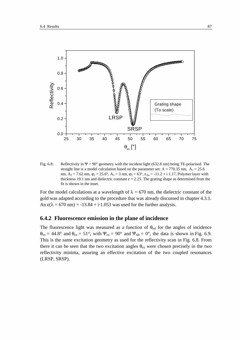
6.4 Results 87
25 30 35 40 45 50 55 60 65 70 750.0
0.2
0.4
0.6
0.8
1.0
SRSP
LRSP
Grating shape (To scale)
Re
flect
ivity
θin [°]
Fig. 6.8: Reflectivity in Ψ = 90° geometry with the incident light (632.8 nm) being TE-polarised. Thestraight line is a model calculation based on the parameter set: Λ = 770.35 nm, A1 = 25.6nm, A2 = 7.62 nm, ϕ2 = 25.6°, A3 = 3 nm, ϕ3 = 63°, εAu = -11.2 + i 1.17, Polymer layer withthickness 19.1 nm and dielectric constant ε = 2.25. The grating shape as determined from thefit is shown in the inset.
For the model calculations at a wavelength of λ = 670 nm, the dielectric constant of thegold was adapted according to the procedure that was already discussed in chapter 4.3.1.An ε(λ = 670 nm) = -13.84 + i·1.053 was used for the further analysis.
6.4.2 Fluorescence emission in the plane of incidence
The fluorescence light was measured as a function of θrel for the angles of incidenceθex = 44.8° and θex = 51°, with Ψex = 90° and Ψtilt = 0°, the data is shown in Fig. 6.9.This is the same excitation geometry as used for the reflectivity scan in Fig. 6.8. Fromthere it can be seen that the two excitation angles θex were chosen precisely in the tworeflectivity minima, assuring an effective excitation of the two coupled resonances(LRSP, SRSP).

88 6 Fluorescence in the field of coupled surface resonances
25 30 35 40 45 50 55
0
2000
4000
6000
8000
10000
12000
θex
= 44.8° LRSP θ
ex = 51° SRSP
to be disregarded
Flu
ores
cenc
e In
tens
ity [
a.u.
]
θrel
[°]
Fig. 6.9: Fluorescence intensity as a function of the emission angle θem (= θrel) at Ψem = 90° for twodifferent excitation angles θex. The excitation wavelength equals λex = 632.8 nm. When thespecular reflection of the incoming beam coincides with the detection axis, there is someundesired stray light reaching the detector. These data points are drawn as crosses and shouldnot be considered for the analysis.
The emitted intensity shows two clear maxima which are attributed to surfaceresonances corresponding to the emission wavelength of the chomophore (670 nm).They occur at θrel = 37.5° and θrel = 43.5°. The positions where mimima are observed ina reflection experiment with the corresponding wavelength λem = 670 nm (compare themodel calculation in Fig. 6.3) coincide well with the positions of these emission peaks.Therefore, they can be attributed to an enhanced emission that is mediated by the twocoupled resonances at λem = 670 nm.
An important observation can be made regarding the relation between the maximumvalues of the two peaks for the two excitation angles. Excitation of the LRSP (atλ = 632.8 nm) leads to an enhanced fluorescence emission mediated by the LRSP(θrel = 37.5° at λ = 670 nm). The same holds for the SRSP. The transfer from excitationto fluorescence energy is more effective between coupled resonances of equal type thanbetween different types. This effect can be explained with the concept of the site-dependent variation of the excitation and emission probability as introduced in section6.1.3.2.
In order to quantify this effect, the ‘Correlation number’ C is defined as

6.4 Results 89
C
II
II
LRSPLRSP
SRSPLRSP
LRSPSRSP
SRSPSRSP
= ( 6.16 )
where I denotes the maximum intensity of the peak as it is read from the plot and thesuperscript/subscript indicate whether the excitation/emission angle corresponds to theLRSP or SRSP coupled resonance. In the present case (Fig. 6.9) a correlation number ofC = 2.12 is found.
Some remarks must be made about the experimental errors.
The final angular resolution of the detector leads to a smearing out both in direction ofθrel (which will broaden the narrower peak at 37°) and in Ψtilt (which will lead to agenerally diminished effect as will be shown in the next section). The finite wavelengthresolution of the detector has a similar effect. For these reasons, it can be assumed thatthe ‘real’ correlation number is higher than the one that was determined from theexperimental data.
Outside the resonance region a significantly higher signal is measured than predicted bathe calculation (compare the following section). This effect may be attributed toscattering effects due to roughness features on the grating surface. This background willagain lead to a reduction of the correlation number as found from the measurement. Onemay eliminate this background by subtracting a constant number from the data, but thisdoesn’t give satisfying results in the region around θrel = 50°.
It is not meaningful to attempt to quantify all these effects especially the error that isinduced by scattering. Therefore, no error is assigned to the measured correlation. Itshould be kept in mind, though, that it can be assumed that the measured correlation istoo low.
6.4.3 Detection in the plane of incidence: model calculations
Calculations based on the two models introduced in section 6.2, ‘quickly rotatingdipoles’ and ‘fixed dipoles’ were performed. The calculated fluorescence intensities forboth models are compared to the measured data in Fig. 6.10. A scaling factor wasapplied to the calculated data to obtain a better correspondence to the measurement(Note: A scaling factor won’t change the correlation as defined in equation ( 6.16 ))

90 6 Fluorescence in the field of coupled surface resonances
25 30 35 40 45 50 55
0
2000
4000
6000
8000
10000
12000
SRSPLRSP
(a)
measured fixed rotating
Flu
ores
cenc
e In
tens
ity [
a.u.
]
θrel [°]
25 30 35 40 45 50 55
SRSPLRSP
(b)
measured fixed rotating
θrel [°]
Fig. 6.10: The measured data for (a) θex = 44.8° ( excitation with the LRSP) and for (b) θex = 51°(excitation with the SRSP) together with model calculations based on the model of fastrotating dipoles (narrow black line) and fixed dipoles (broad grey line).
Calculations based on both models predict a significant correlation. The correlationnumber that is found for the rotating dipoles is 1.79, smaller than the one experimentallydetermined (C = 2.12). The fixed dipoles on the other hand predict a correlation numberof 2.93 which is too high. Since the two averaging procedures may be regarded asextreme cases, it is not surprising that neither is able to give a perfect description of themeasured data. Furthermore, as was pointed out in chapter 3, the roughness of thesample induces some uncertainties in the grating profile as determined from reflectivitymeasurements. Therefore, the intensity distributions as determined from the modelcalculations will have some degree of uncertainty, also.
To conclude, both averaging procedures predict a correlation of the order of magnitudethat is observed experimentally. Since all experimental errors lead to a diminishedcorrelation, it can be assumed that the model of quickly rotating dipoles is notapplicable for the measurement on this system. Due to the errors in the measurementand in the modelling, a quantitative evaluation is not possible. Still, the approximateagreement between experiment and theory gives good insight into the underlyingphysics.
6.4.4 Emission outside the plane of incidence
More fluorescence data were recorded with the detector being positioned outside theplane of incidence (Ψtilt ≠ 0°, therefore Ψem ≠ 90°,). These experiments track theresonance features involved in the outcoupling process in their evolution from coupledresonances (at Ψtilt = 0° ) to ‘free’ surface plasmons for higher Ψtilt. (compare Fig. 6.3

6.4 Results 91
and Fig. 6.5). It is expected that the correlation number for an outcoupling processwhich is mediated by free surface plasmons will approach 1 (no correlation) due to thefact that they do not have a field localisation. Fig. 6.11 shows data measured with thedetector moved out of the plane of incidence by Ψtilt = 1.6° and Ψtilt = 5.5°
30 35 40 45 50 55
0
2000
4000
6000
8000
10000
12000
(a)
θin = 44.8° (LRSP)
θin = 51° (SRSP)
Flu
ores
cenc
e In
tens
ity [a
.u.]
θrel
[°]
15 20 25 30 35 40 45 50 55 60 650
2000
4000
6000
8000
(b)
θin = 44.8°
θin = 51°
θrel
[°]
Fig. 6.11: Fluorescence intensity at Ψtilt = 1.6° (a) and at Ψtilt = 5.5° (b) for the two different angles ofincidence corresponding to the excitation of the LRSP and the SRSP.
The distance between the two peaks increases with increasing Ψtilt as it is expected fromFig. 6.3, while their mutual coupling weakens. For small tilting angles (Ψtilt = 1.6°)these resonances transition from coupled to free surface plasmons, for Ψtilt = 5.5°, theresonances are some distance from the ‘photonic band gap’ and can therefore beregarded as free surface plasmons.
It is clearly seen that the difference in shape between the two data sets is still visible forΨtilt = 1.6° while at Ψtilt = 5.5° the two sets of data appear nearly identical up to aconstant scaling factor. This is reflected in the correlation number at Ψem = 1.6° ofC = 1.96 which is already diminished from C = 2.12 in the plane of incidence, showingthat the field confinement is already diminished. For Ψem = 5.5° the correlation numberis determined as 1.024 which is equal to 1 within the experimental error.
The correlation numbers that were obtained from several out-of-plane measurements,including the two that were just presented are shown in Fig. 6.12. For comparison,correlation numbers that were obtained by model calculations based on the two modelsare also shown.
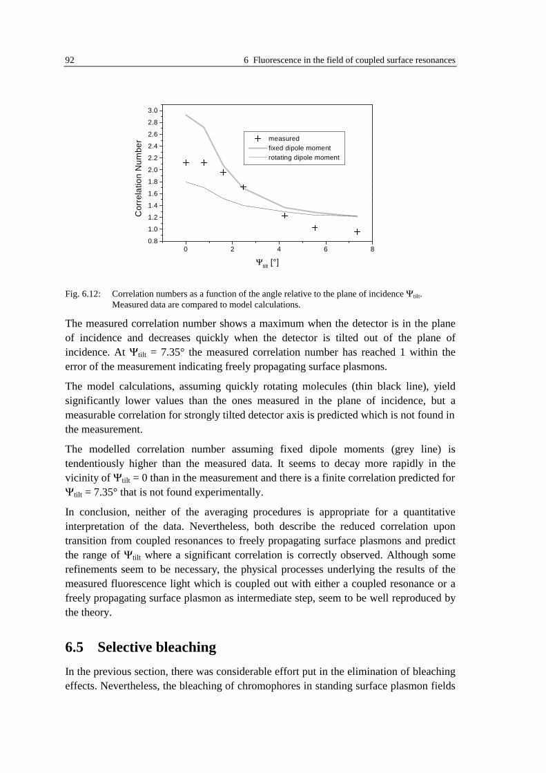
92 6 Fluorescence in the field of coupled surface resonances
0 2 4 6 80.8
1.0
1.2
1.4
1.6
1.8
2.0
2.2
2.4
2.6
2.8
3.0
measured fixed dipole moment rotating dipole moment
Cor
rela
tion
Nu
mbe
r
Ψtilt [°]
Fig. 6.12: Correlation numbers as a function of the angle relative to the plane of incidence Ψtilt.Measured data are compared to model calculations.
The measured correlation number shows a maximum when the detector is in the planeof incidence and decreases quickly when the detector is tilted out of the plane ofincidence. At Ψtilt = 7.35° the measured correlation number has reached 1 within theerror of the measurement indicating freely propagating surface plasmons.
The model calculations, assuming quickly rotating molecules (thin black line), yieldsignificantly lower values than the ones measured in the plane of incidence, but ameasurable correlation for strongly tilted detector axis is predicted which is not found inthe measurement.
The modelled correlation number assuming fixed dipole moments (grey line) istendentiously higher than the measured data. It seems to decay more rapidly in thevicinity of Ψtilt = 0 than in the measurement and there is a finite correlation predicted forΨtilt = 7.35° that is not found experimentally.
In conclusion, neither of the averaging procedures is appropriate for a quantitativeinterpretation of the data. Nevertheless, both describe the reduced correlation upontransition from coupled resonances to freely propagating surface plasmons and predictthe range of Ψtilt where a significant correlation is correctly observed. Although somerefinements seem to be necessary, the physical processes underlying the results of themeasured fluorescence light which is coupled out with either a coupled resonance or afreely propagating surface plasmon as intermediate step, seem to be well reproduced bythe theory.
6.5 Selective bleaching
In the previous section, there was considerable effort put in the elimination of bleachingeffects. Nevertheless, the bleaching of chromophores in standing surface plasmon fields

6.5 Selective bleaching 93
is an interesting phenomenon by itself and will be studied in this section. As anapplication, a modification of the FRAP (fluorescence recovery after photobleaching)technique [Axe76] will be presented as a possible application and a proof of principlethereof will be given.
6.5.1 Observation of the selective bleaching
The photonic energy that is absorbed by a dye molecule may cause a photochemicalreaction which transforms the dye into some non-fluorescent molecule. As aconsequence, the fluorescence of a given sample will decrease with time underillumination. Obviously, when the chromophores are exposed to a spatially modulatedelectrical field pattern as it is generated by coupled surface resonances, the bleachingwill mainly occur to the chromophores that are exposed to high field intensities. Thiswill lead to a modulated chromophore density across the grating with the samemodulation period as the electrical field, 385 nm in the present case.
The existence of such a modulation can be proved by following the fluorescenceintensity as a function of excitation and emission angle with time. Because the bleachingis relatively fast, only the two excitation angles (LRSP: θex = 44.8°, SRSP: θex = 51°)and two emission angles (LRSP: θem = 37.5°, SRSP: θem = 43.5°) are chosen that assuremaximum coupling of (incident or emitted) light to the coupled surface resonances.These four intensities are measured while the sample is illuminated under θbleach. Whenthe θbleach is chosen to coincide with maximum excitation of the one resonance, thecorresponding emission can be measured in situ during the bleaching process. Themeasurement of the emission excited by the other resonance requires a short interruptionof the bleaching process as well as bleaching at a ‘wrong’ excitation angle. Bleachingintervals of 5 minutes were chosen opposed to data acquisition times of 10 seconds perpoint to minimise the effect of bleaching at a wrong angle. During the time when thegoniometer positions were changed, the laser beam was blocked from reaching thesample. Fig. 6.13 shows the four peak intensities for bleaching under θbleach = 44.8°(excitation of the LRSP) with λex = 632.8 nm. It is clearly seen that the decay ofILRSP
LRSP is the most rapid, followed by ISRSPLRSP and ILRSP
SRSP, which are approximatelyequal. ISRSP
SRSP exhibits the slowest decay. I denotes the fluorescence intensity, thesuperscript the excitation and the subscript the emission direction.

94 6 Fluorescence in the field of coupled surface resonances
0 20 40 60 80 100 1200
30
60
90
ISRSP
SRSP
ILRSP
SRSP
ISRSP
LRSP
ILRSP
LRSP
Flu
ore
sce
nce
Inte
nsi
ty [
a.u
.]
Exposure time [min]
Fig. 6.13: Evolution of the intensities ILRSPLRSP, ILRSP
SRSP, ISRSPLRSP, ISRSP
SRSP, during illumination in theLRSP. The curves were normalised to a starting value of 100 to allow better comparison.
This behaviour can be explained qualitatively when we consider which molecules areinvolved in which fluorescence process:
1. ILRSPLRSP mainly involves the molecules in the intensity maxima of the LRSP..
2. ISRSPSRSP mainly involves the molecules in the intensity maxima of the SRSP..
3. ILRSPSRSP and ISRSP
LRSP mainly involve the molecules which experience significantfield strength of both coupled resonances, this is dirctly in the slopes of the intensitydistributions in Fig. 6.5.
Because the bleaching rate is proportional to the local electric field strength, thedifferent bleaching rates that are observed in Fig. 6.13 can be understood with theassumption that the chromophores positioned in the intensity maxima of the LRSP willbe most effectively bleached. Indeed, the bleaching beam ‘burns’ a modulation inchromophore density and this effect can be tracked by observation of the fluorescenceintensities at the experimental geometries specified above.
6.5.2 A new ‘FRAP’ method
The spatially selective and irreversible bleaching of fluorescing molecules can be usedfor the study of dynamic processes in thin films. This technique is called ‘FluorescenceRecovery after Photobleaching’ (FRAP) [Axe76]. A high intensity laser is focused on a

6.5 Selective bleaching 95
surface containing chromophores. Soon, all fluorescing molecules in the focal point areirreversibly bleached. After the bleaching laser is switched off, the fluorescence fromthis spot is measured as a function of time. Molecules that were outside the spot at thefirst laser flash are still intact and while they diffuse into the bleached spot, thefluorescence intensity that is detected from there will rise from 0 immediately after thebleaching, ideally back to its original value. The time that is needed for this processdepends on the diffusion constant of the chromophores and allows therefore the study ofdynamic processes in the film.
Exploiting the effect of selective bleaching that was introduced in the last section, a verysimilar experiment can be performed. It may offer the possibility to measure systemsthat are not accessible with conventional FRAP for two reasons:
1. The light cone of a focused laser can be thought of as being composed of plane lightwaves that form an intensity minimum right at a metal surface due to destructiveinterference of the incoming and outgoing beams. Manipulation and investigation offluorescing molecules directly on a metal surface is therefore difficult. In contrast, thecoupled resonances on a diffraction grating have their maximum intensity at the surfaceand are therefore better suited for the investigation of metal-based systems.
2. The average distance x that a molecule diffuses within the time t is given by thediffusion coefficient D [Ger82]:
x D t2 = ⋅ ( 6.17 )
If small diffusion coefficients are to be measured within reasonable time, theobservation of small distances is required. Since the modulation in chromophore densitythat is produced by coupled modes has a pitch of less that 400 nm, very slow processescan be resolved with this technique.
As a proof of principle, the mobility of Cy5 labelled streptavidin dispersed in a film ofPoly(vinylalcohol) is investigated. Fig. 6.14 shows the measured fluorescence intensitiesISRSP
SRSP and ILRSPLRSP, which exhibit the strongest difference in bleaching rate for a
sample that was bleached for 20 minutes at θex = 52.6° (SRSP)10. As in the previoussection, both intensities decrease, this time, ISRSP
SRSP about twice as fast as ILRSPLRSP.
When the bleaching laser is switched off, only a slow change in intensity is observedwhich can be attributed to the photobleaching during the measuring process. Then, att = 55 min, the humidity of the air next to the sample is increased for a few seconds to100% by placing a sponge with hot water close to the sample.
10 This measurement was done on a different sample, therefore the angular positions of the excitation /
emission maxima are slightly shifted.

96 6 Fluorescence in the field of coupled surface resonances
0 20 40 60 80 10050
60
70
80
90
100 Treatment withhumid air
bleaching
ILRSP
LRSP
ISRSP
SRSP
Flu
ores
cenc
e In
tens
ity [a
.u.]
time [min]
Fig. 6.14: The development of the normalised fluorescence intensity which is due to excitation andemission either mediated by the LRSP (open circles) or the SRSP (full squares). First, thesample was bleached in the SRSP for 20 minutes then, after some time the sample wasexposed to humid air for a few seconds.
After this, an increase in ISRSPSRSP, along with a decrease in ILRSP
LRSP indicates theredistribution of the dye molecules. Both (normalised) intensities being almost equal atthe end shows that the dye molecules are distributed completely random again after theexposure to humidity.
Poly- (vinyl alcohol) is a strongly hydrophilic polymer which takes up water from thesurrounding. This swelling causes considerable enhancement of the mobility of thesystem. This gave the chromophores the mobility to rearrange and form a homogenousdistribution again within the polymer layer. By this, it was demonstrated that theredistribution of fluorescent dyes can in principle be tracked by observing thefluorescence intensity which is mediated by coupled resonances in the excitation and theemission processes.
6.6 Conclusion and outlook
It is demonstrated that the localisation of the near field of coupled surface resonancesleads to spatially inhomogenous excitation and emission probabilities of fluorescencemolecules near the surface. A theoretical model allows a quantitative description ofthese effects but due to errors both in the model and in the measurement, a quantitative

6.6 Conclusion and outlook 97
description is not possible. Outcoupling mediated by free surface plasmons does notshow spatial selectivity.
Furthermore, it is shown that the chromophores at the positions of maximum fieldstrength are preferentially bleached. The observation of moisture-induced mobility ofchromophores in a thin polymer layer shows that the effect of selective bleaching can beused for the study of diffusion phenomena.
It would be very interesting to do similar measurements with freely rotatingchromophores as opposed to fixed ones and check if the theoretically expected reductionof the correlation upon enhanced mobility can be observed. The search for spatialinhomogenities of lifetimes and spectral properties due to coupled surface waves wouldbe another interesting problem.
Some more effort should be made regarding the measurement of diffusion effects. Forexample, the research on metal based model membranes (compare e. g. [Gyö99]), whereeither the lipids or proteins could be fluorescence labelled, may benefit from thistechnique.

7 The polarisation dependence of the coupling to thesurface plasmon resonance
7.1 Introduction
The excitation of surface plasmons by light requires the formation of a periodic chargedensity fluctuation in the metal. As it will be shown in detail later (7.4.1), the electricalfield of TE polarised light cannot produce a surface charge on a plane metal surface andon a relief grating in the classical mount. For this reason, coupling to the surfaceplasmon resonance is only possible with TM polarised light in these geometries. In thegeneral case of grating coupling (conical mount, Ψ arbitrary), it is not straightforward tosee which polarisation couples to the surface plasmon resonance. Fig. 7.1 shows themeasured reflectivity as a function of the angle of incidence (given by θ and Ψ) for TMand TE polarisation. A definition of the angles that are used here is given in chapter 2.There, the position of the surface plasmon resonance in the θ-Ψ plane was alreadydiscussed, this problem is analysed in literature as well [Wat97c]. Here, the focus lies onthe polarisation dependence.
7060504030201000
20
40
60
80
TM
Polar angle θ [°]
Azi
mut
hal a
ngl
e ψ
[°]
0 10 20 30 40 50 60 700
20
40
60
80
TE
Azi
mut
hal a
ngl
e ψ
[°]
Polar angle θ [°]
Fig. 7.1: Measured reflectivity of a Λ = 773.6 nm grating for different azimuthal angles. Thewavelength of the incident beam was λ = 632.8 nm. The image on the left was recorded withTM polarised light, right with TE polarisation.
While in the classical mount (Ψ = 0°), there are two clear minima visible that are due tocoupling to the surface plasmon resonance in +1st and -2nd order for TM polarisation, nominimum is observed for TE as expected. When the azimuthal angle is graduallyincreased, the coupling strength of TM weakens while coupling becomes possible withTE. At Ψ = 90°, when the plane of incidence is parallel to the grating grooves, from

7.2 Experimental results 99
momentum matching, two resonances are allowed, +1st and -1st order11. They are excitedby TE-light only. The question that will be treated in more detail in this chapter is: atwhich polarisation of the incident light do minima appear that are due to coupling to thesurface plasmon resonance?
In the next section (7.2), measurements of the surface plasmon resonance for differentlinear polarisations are presented. These measurements are compared to thecorresponding model calculations in section 7.3. Subsequently, some more calculationsdeal with the case of an almost perfectly conducting metal. As a next step (7.4), thepolarisation dependence of surface plasmon coupling is discussed on a geometricalbasis. Finally, an analysis of the polarisation of the reflected beam (7.5) stresses theimportance of a full analysis of the polarisation state.
7.2 Experimental results
The grating that was investigated with respect to its polarisation dependence wasoptically characterised. Since exactly this grating served as an example to illustrate theprocedure of optical characterisation in chapter 3.3, the results that were obtained thereare valid for the following analysis.
As a next step, this grating was investigated with respect to the polarisation-dependenceof surface plasmon coupling in the conical mount.
It was already seen in the introduction that in the classical mount, there are no minima inthe reflected intensity when the sample is illuminated with TE-polarised light. Similarly,TM-light does not lead to minima in the reflectivity at Ψ = 90°. For all other Ψ, bothTM and TE do couple to some extent. An arbitrary linear polarisation p is described as asuperposition of a TM and a TE component (Compare Fig 2.4) which have directionsthat are defined by the unit vectors pTM and pTE.
( ) ( )p p pTM TE= ⋅ +cos sinϕ ϕ ( 7.1)
with the ‘polarisation angle’ ϕ. In Fig. 7.2, the θ-dependent reflectivity is shown for ϕvarying from 0° to 180° for one example (Ψ = 79°) as obtained from a measurement.
11 To be precise, at Ψ = 90° no free surface plasmons but coupled resonances are observed, but this does
not influence the polarisation dependence.
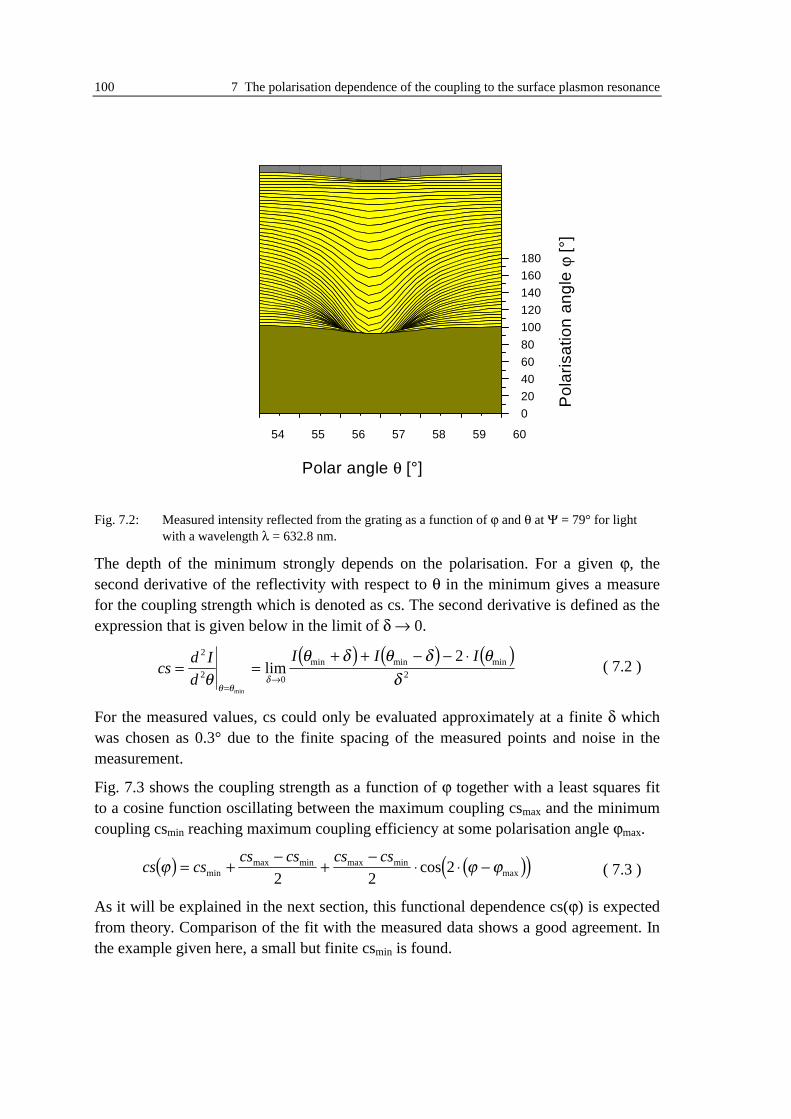
100 7 The polarisation dependence of the coupling to the surface plasmon resonance
54 55 56 57 58 59 60
0
20
40
60
80
100
120
140
160
180
0.010
0.015
0.020
Pol
aris
atio
n a
ngl
e ϕ
[°]
Polar angle θ [°]
Fig. 7.2: Measured intensity reflected from the grating as a function of ϕ and θ at Ψ = 79° for lightwith a wavelength λ = 632.8 nm.
The depth of the minimum strongly depends on the polarisation. For a given ϕ, thesecond derivative of the reflectivity with respect to θ in the minimum gives a measurefor the coupling strength which is denoted as cs. The second derivative is defined as theexpression that is given below in the limit of δ → 0.
( ) ( ) ( )cs
d I
d
I I I= =
+ + − − ⋅
=→
2
2 0 2
2
θθ δ θ δ θ
δθ θ
δmin
lim min min min ( 7.2 )
For the measured values, cs could only be evaluated approximately at a finite δ whichwas chosen as 0.3° due to the finite spacing of the measured points and noise in themeasurement.
Fig. 7.3 shows the coupling strength as a function of ϕ together with a least squares fitto a cosine function oscillating between the maximum coupling csmax and the minimumcoupling csmin reaching maximum coupling efficiency at some polarisation angle ϕmax.
( ) ( )( )cs cscs cs cs cs
ϕ ϕ ϕ= +−
+−
⋅ ⋅ −minmax min max min
maxcos2 2
2 ( 7.3 )
As it will be explained in the next section, this functional dependence cs(ϕ) is expectedfrom theory. Comparison of the fit with the measured data shows a good agreement. Inthe example given here, a small but finite csmin is found.

7.3 Numerical calculations 101
0 50 100 150 2000.0000
0.0005
0.0010
0.0015
0.0020
csmax=0.00171
ϕmax = 73.9°
ψ = 79°
θmin = 56.7°
csmin = 0.00003
d2 I/dθ2 [a
.u.]
Polarisation angle ϕ [°]
Fig. 7.3: The coupling strength cs is plotted in the minimum of the plasmon resonance (θ = 56.7°) as afunction of the polarisation angle ϕ. The straight line is a fit according to equation ( 7.3 ).
7.3 Numerical calculations
7.3.1 Mathematical description of the polarisation
These experimental results are now compared to model calculations. This required theextension of the numerical code (compare chapter 2) to incident light of anypolarisation, which means that the incident and outgoing beam are described as a planewave with the electrical field which is varying in space (x) and time t.
( ) ( ) ( )( )E x p p k xTM TE, expt E E i tTM TE= ⋅ + ⋅ ⋅ ⋅ ⋅ − ⋅ω ( 7.4 )
where k is the wavevector. The unit vectors pTM and pTE are describing the directions ofthe fundamental polarisations, the corresponding amplitudes of the electrical field arelabelled ETM and ETE. In the most general case of elliptical polarisation, theseamplitudes will take complex values, for linear polarisation they can be chosen as realnumbers and may be expressed by the polarisation angle ϕ ( compare with equation (7.1)). It is convenient to define a two-dimensional vector E0 which describes thepolarisation state and intensity of the light,
( )( )E0 =
=
⋅⋅
E
E
E
ETM
TE
0
0
cos
sin
ϕϕ
( 7.5 )
where E0 is the magnitude of the electrical field vector. This representation is used todescribe both the incoming and the outgoing beam. Since the response of the opticalsystem under investigation is assumed to be linear, the connection between incomingand outgoing beam is given by a complex 2-dimensional matrix.

102 7 The polarisation dependence of the coupling to the surface plasmon resonance
E E0out
0in=
⋅
M M
M MTMTM
TETM
TMTE
TETE
( 7.6 )
At this point it can be shown that the fitting function ( 7.3 ) was the appropriate choice.First it is important to note that the dependence of the reflected intensity on the (linear)polarisation angle of the incoming beam will always be sinusoidal in shape because:
( ) ( ) ( )( ) ( )( )( )( ) ( )( )
( ) ( ) ( ) ( )
I E M M
E M M
A B C
outTMTM
TETM
TMTM
TETM
ϕ ϕ ϕ ϕ
ϕ ϕ
ϕ ϕ ϕ ϕ
= = ⋅ ⋅ + ⋅ +
⋅ ⋅ + ⋅
= ⋅ + ⋅ + ⋅ ⋅
E0out 2
0
2
0
2
2 2
cos sin
cos sin
cos sin sin cos
( 7.7 )
with some coefficients A, B, C. Obviously, this expression is a harmonic oscillationwith twice the period of ϕ with some offset and some phase shift. The coupling strengthcs as defined in ( 7.2 ) is a linear combination of intensities and has therefore the samesinusoidal form. As a consequence, ϕmax, csmin and csmax are sufficient to describe thepolarisation dependence.
Some care must be taken with the appropriate chirality of the co-ordinate systems thatare defined by the polarisation vectors and the propagation direction of the beam. Here,(pTM, pTE, k) are chosen as right handed (compare with Fig. 2.4)12
Upon reflection on plane interfaces, by definition, the projection of the electrical fieldvector on the reflecting plane for TM-light has a phase jump of 180° while there is nophase jump for TE-light (compare e. g. [Jac83]). This convention preserves the chiralityof the light beam upon reflection.
With the modelling program ‘oblique’, the matrix elements as defined in equation ( 7.6 )were determined for the appropriate angles of incidence (θ, Ψ). This allowed todetermine the polarisation dependent coupling strength cs(ϕ) according to equation ( 7.2) from model calculations.
7.3.2 Comparison between theory and experiment
The experimental procedure that was described in section 7.2 was repeated for severalazimuthal angles and a fitting as described above allowed the experimentaldetermination of ϕmax, csmin and csmax. The corresponding numerical calculations for thegrating under investigation were also performed.
The values of ϕmax as determined from experiment are compared to the modelled resultsin Fig. 7.4.
12 For the modelling, it was important to transform the vectors because in the original code ‘oblique’ the
chirality is just inversed.

7.3 Numerical calculations 103
For Ψ > 70°, excitation of surface plasmons is possible in two different diffractedorders, +1st and -1st (compare Fig. 7.1), but at different polar angles which is not visiblein this plot because the implicit θ-dependence cannot be plotted in 2 dimensions. Thepolarisation dependent coupling to the surface plasmon resonance in -2nd order is notshown. It can be seen in the plot that the model calculations are well suited to describethe measurement.
0 20 40 60 80 100
0
20
40
60
80
100
Calculation
Experimental +1st order
Experimental -1st order
ϕ max
[°]
ψ [°]
Fig. 7.4: The polarisation angle of maximum coupling ϕmax for the resonances that are found in thereflectivity of light with λ = 632.8 nm on the grating under investigation.
The next parameter of interest is the strength of the polarisation dependence, which isreflected in the ratio cmin/cmax. This number will approach zero if there is a (linear)polarisation where no surface plasmon coupling occurs and approaches 1 if there is nopolarisation dependence of the coupling strength. This number was determined frommodel calculations and from the experiment. The results are compared in Fig. 7.5. Forall possible coupling geometries where the +1st diffracted order is responsible for thecoupling to the surface plasmon, cmin/cmax is very small in the numerical modelling andthe variations in the measured values are due to experimental errors. For coupling in -1st
order, cmin/cmax increases significantly when θ approaches 90° (Ψ → 70°).

104 7 The polarisation dependence of the coupling to the surface plasmon resonance
0 20 40 60 80 100
0.0
0.1
0.2
0.3
0.4
0.5
Calculation
Experimental +1st order
Experimental -1st orderc m
in/c
max
ψ [°]
Fig. 7.5: The value of cmin/cmax in calculation and experiment. The open circles correspond to couplingin +1st order, the full circles to -1st order. The wavelength of the incident light isλ = 632.8 nm.
These results show conclusively that the modelling routine is capable to describe thepolarisation dependence of surface plasmon excitation in good agreement with nature.
7.3.3 Asymptotic behaviour
In order to find out if there is some general principle underlying the polarisationdependence, more model calculations were performed assuming a very shallow grating(A1 = 1 nm) with different pitch Λ on an almost ideal metal (ε = -100 + i 0.1). Thefollowing observations were made in the model calculations:
1. For an ideal metal, cmin/cmax approaches 0. That implies that in this case there is alinear polarisation state that doesn’t show a surface plasmon minimum in its reflectivity.
2. The polarisation angle of optimum coupling ϕmax depends only on the reflectiongeometry (θ, Ψ) and it is completely independent from the coupling order13.
This is surprising at first sight for the following reason: Surface plasmons that arecoupled in different order are described by different in-plane wavevectors or‘propagation directions’. These different wavevectors will lead to differentelectromagnetic field distributions as it can be concluded from equation (2.5).Nevertheless, maximum coupling to plasmons in all orders occurs with the same fielddistribution expressed by the same linear polarisation of the incident beam
3. There is an analytical equation that describes ϕmax(θ, ψ) which has been found byanalysing the model calculations:
13 For any combination of θ, Ψ coupling in any order can be achieved by choosing the appropriate grating
pitch.

7.4 Geometrical discussion 105
( ) ( ) ( )tan tan cosmaxϕ θ= ⋅Ψ ( 7.8 )
In Fig. 7.6, ϕmax(θ, Ψ) is plotted as obtained from numerical calculations together withthe result that is obtained analytically. The small deviations of the real metal gratingfrom the ideal case are due to the fact that gold is not a perfectly conducting metal(finite ε) and that the grating under investigation has a finite amplitude.
0 20 40 60 80 100
0
20
40
60
80
100
Calculation Analytical form
Pol
ariz
aito
n an
gle
ϕ [°
]
ψ [°]
Fig. 7.6: Ψ-dependent ϕmax as obtained with the analytical form ( 7.8 ) in comparison to the results ofthe numerical calculation (λ = 632.8 nm).
7.4 Geometrical discussion
In this section, an attempt is made to develop a geometrical explanation for the resultsthat were found in the previous subsection, especially equation ( 7.8 ). First, anexplanation for the polarisation dependence in prism coupling and in grating coupling inthe classical mount is given. Then, the geometrical interpretations that are found inliterature [Vei95], [Fer93], [Kit96b] are critically reviewed on the basis of a vectorialrepresentation of the experimental geometry that is defined first.
7.4.1 Easy geometries
Excitation of the surface plasmon resonance requires the formation of a modulation incharge density. When a plane electromagnetic wave falls on a grating in the classicalmount, the electrical field is parallel to the grating grooves for TE polarisation as shownin Fig. 7.7. No charge density oscillation may be formed due to this field because thecharges are moved along lines formed of equivalent points of the grating surface whichare exposed to the same time-dependent electrical field. Therefore, for any volumeelement, the number of electrons leaving the volume equals the number of enteringelectrons.

106 7 The polarisation dependence of the coupling to the surface plasmon resonance
On a plane metal surface, the same argument can be applied. In agreement with the wellestablished experimental findings (Kretschmann- and Otto-configuration, comparechapter 2.4), surface plasmon excitation on a planar multilayered system is only possiblewith TM polarised light.
E
xy
zk
Fig. 7.7: The electrical field of a TE-polarised light beam in the classical mount.
7.4.2 Definition of the geometry
The definitions that were presented graphically in Fig. 2.4 are now described in avectorial representation. The Cartesian co-ordinate system that is chosen as a basis forthe description of the problem is right handed and has its x-axis parallel to the reciprocalgrating vector and its y-axis parallel to the grating grooves. The z-axis is normal to thesample surface and is pointing into the dielectric. So, the reciprocal grating vector kg
equals:
k g =⋅
⋅
21
0
0
πΛ
( 7.9 )
The azimuthal angle Ψ is defined as the counterclockwise rotation of the projection ofthe plane of incidence onto the sample surface14, starting with 0 when the reciprocalgrating vector lies in the plane of incidence. The wavevector of the incoming beam, ki,expressed in terms of angles equals therefore
( ) ( )( ) ( )
( )k i = ⋅
⋅⋅
−
k0
sin cos
sin sin
cos
θ ψθ ψ
θ
( 7.10 )
where k0 is the modulus which is fixed by the dispersion relation of light in thedielectric. The linear polarisation of the incoming beam is expressed as thesuperposition of TM and TE polarisation, where the polarisation vector pTE must be
14 In the experiment, this is realised by a clockwise rotation of the grating around its normal.

7.4 Geometrical discussion 107
orthogonal to the plane of incidence which is spanned by ki and the surface normal andcan therefore be calculated as a vector product
( )( )p kTE i∝ ×
∝ −
0
0
1 0
sin
cos
ψψ ( 7.11 )
Normalisation constants are omitted because they are of no significance for the furtheranalysis. The direction of the electrical field for TM polarisation must be orthogonal tothe incident beam and the polarisation vector pTE.
( ) ( )( ) ( )
( )p p kTM TE i∝ × ∝
⋅⋅
cos cos
sin cos
sin
ψ θψ θ
θ
( 7.12 )
7.4.3 Geometrical interpretation
Some investigations of the polarisation (ϕ- ) dependence of the coupling to the surfaceplasmon resonance in the conical mount are found in literature. They are neitherconsistent with each other nor do they satisfactorily describe the experimental findingsthat were presented in the previous chapter.
Fernandez-Horn [Fer93] and Veith [Vei95] claim that maximum coupling requiresΨ = ϕ. This interpretation is clearly wrong as it can be easily verified from equation (7.8 ) as well as in Fig. 7.4.
Kitson et al. [Kit96b] state that ‘At a general value of Φ (which is the azimuthal angle,Ψ in the notation that is used here) it is only the component of the photon E-field that isin the plane defined by the substrate normal and the grating vector that may coupleresonantly to the SPPs (surface plasmon polaritons)’.
One may assume that all components of the electrical field in this plane couple equallywell. In this case, the prerequisite for maximum coupling would be
p ⋅
=0
1
0
0 ( 7.13 )
which yields when ( 7.9 ), ( 7.10) and ( 7.11 ) are plugged in
( ) ( ) ( )tan tan cosmaxϕ θ= ⋅Ψ ( 7.14 )
which is in agreement with the result that was obtained by measurement and numericalmodelling.
But there are two major drawbacks of this model. Firstly, there is in general for any ϕ, anot-vanishing component of the electrical field in this plane because the plane of
108 7 The polarisation dependence of the coupling to the surface plasmon resonance
possible polarisations and the plane spanned by the reciprocal grating vector and thesurface normal are in general not orthogonal. Nevertheless there is a polarisation thatdoes not show a surface plasmon related minimum for an ideal metal (cmin/cmax doesvanish completely).
The second problem concerns the assumption that the electrical field couples with equalstrength no matter how it is oriented in the plane spanned by the reciprocal gratingvector and the surface normal.
In this plane, either fields parallel to the reciprocal grating vector (x-axis) or parallel tothe surface normal (z-axis) may exist. It is not clear why these two components shouldhave the same power to excite charge density oscillations.
Kitson et al. [Kit96b] assume that ‘[...] such an E-field has a component normal to thelocal surface allowing it to couple to the surface charge oscillation that constitutes anSPP’. This point of view does not yield an equally effective excitation of a chargedensity oscillation for all orientations of the E-field inside the plane spanned by the x-and z-axis as it is shown now. A charge ρ that is proportional to the normal componentof the incident electrical field can be calculated for a relief grating which is described asa function z(x) by expressing the local normal vector of the surface in terms of thefunction which is describing the surface.
( )( )[ ]
( )ρ x
z x
z x
∝ ⋅ =+
−
⋅n E E1
10
12
'
'( 7.15 )
For a very weakly corrugated grating, this function can be expanded in a Taylor serieswith respect to z’(x):
( ) ( )[ ]( )( )[ ] ( )[ ]( )
ρ ∝− +
− ⋅ +
⋅z x O z x
z x O z x
' '
' '
2
2 3
0
1 12
E ( 7.16 )
If a very shallow sinusoidal grating is considered, only the x-component of the electricalfield possesses a not-vanishing linear term and does therefore lead to a significantcharge density oscillation that has the appropriate spatial frequency to excite a surfaceplasmon. So, this model is not able to explain an equally good coupling for electricalfields in x- and z-direction. Instead, there would be a polarisation that does not couple atall to the surface plasmon resonance, the one that is orthogonal to kg (x-axis). With theaid of equations ( 7.4 ), ( 7.11 ) and ( 7.12 ) the corresponding polarisation of minimumcoupling can be calculated.
( ) ( ) ( ) ( ) ( )( )rE E⋅
= ⇒ ⋅ − ⋅ ⋅ − ⋅ =1
0
0
0 00 cos cos cos sin sinmin minψ θ ϕ ϕ ψ ( 7.17 )
7.5 Elliptical polarisation 109
From this, with the prerequisite that the ϕ-dependence is sinusoidal (ϕmin = ϕmax + 90),the polarisation of maximum coupling is obtained,
( ) ( )( )tan
tan
cosmaxϕθ
=Ψ
( 7.18 )
which is not in agreement with equation ( 7.8 ).
It must be concluded that the initial assumption that only a local normal component ofthe electrical field may produce a charge density oscillation is wrong. Instead, a locallyvarying tangential component which is parallel to the reciprocal grating vector kg mayproduce a surface charge as well. For a satisfying physical interpretation of thepolarisation dependence of surface plasmon coupling, the coherent superposition of bothof these mechanisms must be taken into account which makes the problem inaccessibleto an easy intuitive interpretation.
So, finally only a heuristic geometrical interpretation is given that describes theexperimental findings but is not based on accurate physical arguments:
‘Whenever the projection of the electrical field vector onto the grating grooves (y-axis)reaches a maximum, no surface plasmon related minimum is observed on an idealmetal.’
It should be noted that the polarisation that does couple best coincides with the E⊥
polarisation which was introduced in a theoretical paper by Li [Li94].
7.5 Elliptical polarisation
It is well known that the full information about a monochromatic plane light waveincludes its polarisation state. A detailed description of the mathematical andexperimental treatment of elliptically polarised light is found in many textbooks,[e.g. Col93].
In the previous sections, only linearly polarised light was considered as excitation and itwas always the full intensity of the reflected beam that was detected. Here, as a remark,the effect of a detection that is polarisation selective is investigated. In Fig. 7.8, it isdemonstrated that a missing minimum in the total intensity of the reflected beam doesnot necessarily imply that there is no interaction between the incident beam and thesurface plasmon resonance. When the TM and the TE-polarised component of thereflected beam are measured separately, resonances are observed in the two individualintensities which are just mutually inverse so that they cancel each other when the sumof the two orthogonal components (full intensity) is measured.

110 7 The polarisation dependence of the coupling to the surface plasmon resonance
12 14 16 18 20 22 240.450
0.455
0.460
0.465
Ref
lect
ivity
θ [°]
0.445
0.450
0.455
0.460
TE
TM
0.915
0.920
0.925 Full intensity
Fig. 7.8: Normalised intensity for ψ = 45°, ϕ = -45°. The first graph shows the full reflected intensitywhile the other two were recorded with a polariser in the reflected beam with the orientationas indicated in the graph. The line shows the corresponding model calculation (λ = 632.8 nm)
It is observed that although the excitation of the surface plasmon resonance has no effecton the total reflected intensity, care must be taken with the statement that there is ‘nocoupling to the surface plasmon resonance’. When the polarisation state of the outgoingbeam is investigated, it is seen that there is still some interaction of the incident lightwith the surface plasmon. The missing plasmon-related minimum must be regarded asan interference effect and cannot be simply explained by regarding the ability of theincident beam to produce a surface charge.
By some more model calculations, the limit of a perfect metal was investigated again. Itturns out that in this limit the resonances in the individual polarisations will vanish.
7.6 Conclusion
In this chapter, the influence of the linear polarisation of the incident beam on the abilityto excite the surface plasmon resonance on a metal grating was investigated. The depthof the minimum in the total intensity of the reflected beam was taken as a measure ofthe coupling strength. Good agreement was found between experiment and numericalmodelling with respect to the polarisation where the resonance minimum is deepest andto the finite ‘minimum coupling’ cmin/cmax. For an ideal metal with a very shallowmodulation, it was found in a set of model calculations that there is a linear polarisationwhich does not show any reflectivity minimum due to coupling to the surface plasmon

7.6 Conclusion 111
and an analytical equation for this polarisation was found which is only dependent onthe polar angle θ and the azimuthal angle Ψ. Approaches to the problem that are foundin literature do not give an appropriate description of the experimental findings. Instead,an alternative heuristic interpretation is proposed. An analysis of the two orthogonalpolarisations of the light reflected from a real metal grating shows that there may besome interaction with the surface plasmon resonance even if no minimum in the totalreflected light intensity is visible.

8 About thin film sensing
8.1 Introduction
The wavevector of the surface plasmon resonance is altered by a thin dielectric film onthe metal surface. This effect has been applied to the investigation of thin films byGordon et al. [Gor77] for the first time. With this ‘surface plasmon spectroscopy’, thedetection and investigation of dielectric films in the Angstrom level on metal surfaces iseasily possible. Today, this technique has become a standard method in biochemistry.Commercial surface plasmon spectrometers are available from several differentcompanies (Pharmacia, BioTul and others). Mostly, prism coupling is used for sensingdue to several reasons:
• The optical response of a flat multilayer system can easily be calculated with thetransfer matrix method (compare chapter 2).
• In in-situ investigations of chemical reactions on the metal surface, usually somesolution will be present on top of the metal. By prism coupling in Kretschmann-configuration (compare chapter 2), the light beam that excites the surface plasmondoes not propagate through this solution and is therefore insensitive toperturbations that may be introduced by stirring or by the addition of light-absorbing species. The only interaction of the light with the solution on top of thesurface that is to be probed is via the evanescent field of the surface plasmon.
• A flat gold surface is a well defined environment for the chemical reactions thatare to be investigated.
Nevertheless there are certain cases where the excitation of the surface plasmon with anoptical grating is favourable. When the appropriate pitch of the grating is chosen, thesurface plasmon resonance is observed only a few degrees off from normal incidence.This was used by Kleideiter [Kle99, Kle00] to investigate thin films under highhydrostatic pressure through a very small and thick window as it is necessary for thestability of the set-up. Other examples where prism coupling is impossible and thereforegrating coupling is the only solution to obtain informations about dielectric films on themetal surface are investigations on liquids with a high refractive index or measurementswhere a substrate material must be used that does not have the required opticalproperties for prism coupling (like simultaneous investigation of optical and rheologicalproperties of a thin film on a quartz microbalance).
In this chapter, it is demonstrated that grating coupling can be used to investigatereactions on metal surfaces. First (8.2), an example for a measurement on a gold gratingis given which proofs the applicability of gratings for sensor purposes. The main focusof this chapter lies on section 8.3 where the evaluation of the measured data is

8.2 Experimental 113
described. First, an evaluation procedure which is based on the precise mathematicaltreatment of the corrugated metal surface is presented. Then, a much simpler evaluationis proposed as an alternative and its applicability is demonstrated.
8.2 Experimental
8.2.1 Experimental set-up
In practice, one is usually interested in dielectric films on metal surfaces that areexposed to a solvent environment containing molecules that build or modify the film.Examples are self assembled monolayers of thiol compounds [Woh99] and the fusion oflipid vesicles on pre-treated gold surfaces [Sch98]. In Fig. 8.1, a cuvette which can beused for such experiments with a diffraction grating is shown. A laser beam passesthrough a glass slide and the solution under investigation. It is reflected on the grating,passes through the solution and the glass again and finally reaches a detector. Thecuvette, being mounted on an optical set-up as described in chapter 3, allows for thevariation of the polar angle of incidence and the measurement of the reflected intensityin a θ / 2θ geometry (tracking of the reflected beam with the detector).
gold gratingO-ring
incoming beam outgoing
beamglass slide
tefloncuvette
θext
θ
rotationaxis
to detector
Fig. 8.1: Sketch of a cuvette for surface plasmon spectroscopy with an optical grating.
Due to the different refractive indices of air and the liquid in the cuvette, the polar angleof the reflection on the gold-liquid interface θ is not equal to the one in air, θext which isfixed externally with the goniometer. Snellius’ law yields in this case
( ) ( )sin sinθ θext sn= ⋅ ( 8.1 )
with the refractive index of the solvent, ns. It is favourable to use a glass slide as coverthat has a refractive index which is as close as possible to ns in order to avoid

114 8 About thin film sensing
interference problems. Cuvette designs that are quite different from the one presented inFig. 8.1 are in use for special purposes. A feature which is common to all the designs isthat the light has to pass through the cover glass and the solvent before and afterreflection on the metal.
8.2.2 Investigation of a thin film
The reliability of a surface plasmon spectrometer which uses an optical grating to couplethe incident light to the surface plasmon resonance is demonstrated in this and thefollowing sections. The well studied15 reaction of octadecanethiol (SH-(CH2)17-CH3)with a gold surface serves as an example. This compound forms a monolayer which isbound covalently to the surface. Fig. 8.2 shows the reflected intensity from a goldgrating before and after the formation of a thiol-monolayer. This process was tracked byrecording the intensity of the reflected beam at a fixed polar angle (θ = 7.5°). Since thisis in the almost linear slope of the resonance, it allows for the on-line observation of ashift of the resonance curve (kinetic mode). Fig. 8.3 shows the reaction kinetics whilethe following experimental procedure was used to form a monolayer of the thiolcompound.
0 2 4 6 8 10 12 14 16 18-0.1
0.0
0.1
0.2
0.3
0.4
0.5
0.6
0.7
0.8
before after
Re
flect
ed
inte
nsi
ty [
a.u
.]
θ[°]
Fig. 8.2: θ-dependent reflectivity of a gold grating before and after the self-assembly ofoctadecanethiol which was dissolved in ethanol. The angle where the intensity was recordedduring the self-assembly (θ = 7.5°) is indicated with a straight line.
The cuvette volume was filled with pure ethanol, subsequently it was rinsed twice withpure ethanol to check the stability of the system. In the kinetic curve, some perturbationdue to the liquid exchange are visible but the system recovers within a few seconds. Itcan be concluded that no artefacts are introduced by the rinsing procedure.
15 An overview over this topic can be found for example in the book of Ulman [Ulm91].

8.3 Evaluation procedures 115
Then, the cuvette was filled with a solution of the thiol in ethanol (5×10⁻⁴ mol/l). Asteep rise in intensity shows the formation of a dielectric film in the self-assemblyprocess.
0 200 400 600 800 1000 1200 1400 16000.054
0.056
0.058
0.060
0.062
Ethanol
Ethanol
Thiol solutionre
flect
ed
inte
nsi
ty [
a.u.
]
time [s]
Fig. 8.3: Reflected intensity at θ = 7.5° during the formation of a monolayer of octadecanethiol.
After the intensity had reached a plateau indicating the end of the adsorption process,the sample was rinsed again, once with thiol solution and once with ethanol, before thesecond reflectivity scan as function of θ was recorded. In this second scan, as expected,a significant shift of the surface plasmon resonance to higher θ is observed (compareFig. 8.2).
8.3 Evaluation procedures
In this subsection, two evaluation routines are presented that can be used to extractinformation about the adsorbed film from reflectivity measurements with the aid of theexample that was introduced above. The optical model system that is used for thedescription of the measurement is drawn schematically in Fig. 8.4.
metal
subphase adlayer
Fig. 8.4: The multilayer system under investigation.

116 8 About thin film sensing
On top of an infinitely thick corrugated metal surface, there is a thin and homogenousfilm, the adlayer, followed by another infinitely thick medium, the subphase. It is theaim of surface plasmon spectroscopy, to determine the thickness of the adlayer from thecomparison between the reflectivity curves before and after the self assembly.
There is one major difficulty with the determination of the thickness of dielectric filmswith surface plasmon spectroscopy. Completely identical resonance curves may beobtained by a whole set of thickness’ and refractive indices. A thin film with highrefractive index cannot be distinguished from a thick film with low refractive index,therefore only one of these two parameters can be measured, the other one must bedetermined otherwise. Usually, the refractive index of the material under investigation isassumed as a constant. Its value may be derived from bulk measurements for materialswhere this is possible. In the case that is treated here, there is no bulk analogue to thethiol monolayer, therefore the same choice is made as in [Fla98], n = 1.5, in order toallow a comparison to the results that were obtained there. For the following, it must bekept in mind that the thickness that is derived from the measurements depends on thechoice for the refractive index.
It should be noted further that the assumption of one homogenous layer which ischaracterised by one dielectric constant is not necessarily a good description of reality.For example dielectric films with holes which are smaller than the wavelength of lightwill mimic a homogenous dielectric film with a reduced thickness.
8.3.1 Rigorous modelling of the grating
The straightforward method to obtain the thickness of the adsorbed layer from anexperiment like the one that was presented above consists in the determination of allparameters that describe the optical response of the bare grating. The refractive index ofthe subphase is easily determined from the position of the pseudocritical edge. With theroutine that is described in chapter 3, the dielectric constant of the gold as well as thegrating profile can be determined from a least squares fit. Fig. 8.5 shows the measureddata and the fit. Some discrepancy is visible for very small θ which is due to light that isreflected from the cover glass and reaches the detector close to normal incidence only.In order to determine the thickness of the thiol layer, a second fit is performed to thereflectivity that was recorded after addition of the thiol where the only free parameter isthe thickness of the thiol layer with an assumed refractive index of n = 1.5.
Changing this parameter shifts the minimum position of the modelled surface plasmonresonance. The changes in the form of the reflectivity curve as observed in Fig. 8.2(mainly deepening and broadening of the resonance) cannot be explained with thismodel as it can be concluded from the difference between the data and the fit in Fig. 8.5(b). This indicates that reality is different from the idealised picture (Fig. 8.4) which wasthe basis for this evaluation routine. Random roughness of the grating surface orinhomogenity of the adlayer may be responsible for this discrepancy.

8.3 Evaluation procedures 117
-2 0 2 4 6 8 10 12 14 16
0.0
0.2
0.4
0.6
0.8
1.0
Experiment Calculation
(a)
θ [°]
Λ = 479.8 nm
A1 = 30.03 nm
A2 = 3.116 nm ϕ
2 = 90°
A3 = 0.93 nm ϕ
3 = 0°
εAu
= -9.878 + 1.972 × i
Re
flect
ivity
θ [°]0 2 4 6 8 10 12 14 16 18
(b)
Fig. 8.5: (a) Measured reflectivity (circles) of the bare gold grating with a fit (straight line) based onthe parameters that are shown in the inset.(b) Measured reflectivity with an additional thiol monolayer (circles) with a modelcalculation including a dielectric adlayer with a thickness of 2.4 nm and a refractive index ofn = 1.5. A better comparison of the two measured data sets is possible in Fig. 8.2
From this fit, the thickness of the dielectric layer was determined as 2.4 ± 0.1 nm, whichis in agreement with literature. The apparent higher thickness of the layer that isreported by Ulman [Ulm91] is due to the lower refractive index (1.45 instead of 1.5)that is used there. When the same refractive index is used, consistent values are obtained[Fla98].
It can be concluded that although the changes in the form of the curve cannot bedescribed by the addition of a single homogenous dielectric layer, the shift of theposition of the surface plasmon minimum yields a film thickness that is consistent withother measurements. It is cumbersome to use this evaluation technique that is based onthe complete characterisation of the grating. This procedure requires much time andcomputer power to perform the initial fit which, at the end, is not able to reproduce themeasured reflectivity perfectly but is only used as a mean to determine the shift of aresonance curve. The following section introduces an easier routine to calculate thethickness of an adsorbed layer from the change of the minimum position.
8.3.2 Evaluation by transformation
In grating coupling experiments, the excitation of a surface plasmon resonance isaccomplished by matching its momentum with a higher diffracted order of the incidentlight beam. In prism coupling, a plane light wave in a high index medium has therequired momentum. These two alternatives are schematically depicted in Fig. 8.6.

118 8 About thin film sensing
prism
metal
kgsubphase
Fig. 8.6: Sketch of two processes to excite a surface plasmon on an subphase-metal interface: gratingcoupling and prism coupling.
While the determination of the thickness of a thin adlayer from a grating-couplingexperiment is difficult, the evaluation of a prism-coupling experiment is easily donewith the transfer matrix algorithm (compare chapter 2 or [Kar91]). If it can be assumedthat the introduction of a coupling of the surface plasmon to light does not change itsmomentum, the momentum change due to a dielectric adlayer ∆k will be the same forboth experiments. This was assumed by Knoll et al. [Kno81] who evaluated data thatwere obtained by grating coupling calculating an equivalent prism coupling geometry.
In reality, the effect of the additional loss channels that are introduced by the finitethickness of the gold layer in prism coupling or by the grating topology in gratingcoupling are not negligible. It is the aim of this section to show that the evaluation of agrating coupling experiment as flat multilayer system yields the right thicknesses inspite of this fact.
As a first step, a transformation is made from the polar angle θgrat of the gratingcoupling experiment to an angle θpris that would yield the same in-plane wavevector kx
in a prism coupling experiment as it is obtained in reality in the first diffracted order.
( ) ( )k n k k n kg s grat x p pris+ ⋅ ⋅ = = ⋅ ⋅0 0sin sinθ θ ( 8.2 )
Here kg is the reciprocal grating vector, ns and np the refractive index of the subphaseand the prism, respectively, and k0 the wavevector of the light in vacuo. In Fig. 8.7 thesame data set as in Fig. 8.5 is shown where θpris is calculated for a hypothetical prism-coupling measurement. The model calculation of the bare gold grating is based on themodel of a planar 3-layer system (prism/gold/subphase) with the parameters as shown inthe graph.

8.3 Evaluation procedures 119
19 20 21 22 23 24 25
0.0
0.2
0.4
0.6
0.8
1.0(a)
θpris
[°]
Prism: d = ∞ ε = 16
Gold: d = 42.7 nm ε = -8.05 + i 1.5
Ethanol: d = ∞ ε = 1.85
Experiment Calculation
Re
flect
ivity
θpris
[°]
19 20 21 22 23 24 25
(b)
Fig. 8.7: The same set of data as in Fig. 8.5, transformed to a ‘hypothetical prism scan’ with a prism ofrefractive index np = 4.(a) Experimental data from the pure gold surface. The straight line is a model calculation of amultilayer system as specified in the inset.(b) Experimental data after the self-assembly. The modelling assumes an additionaldielectric layer with a thickness of 2.3 nm and a refractive index of 1.5.
It is clear that the fit is pretty poor compared to the results that were obtained byrigorous modelling, especially close to the pseudocritical edge. Nevertheless, it ispossible to reproduce the position and shape of the minimum rather well. In the modelcalculation on the right, the additional thiol layer was modelled with an assumedn = 1.5. The thickness was varied to give an optimum fit to the data. Within the error thesame thickness is found with this technique as with the rigorous approach, d = 2.3 ± 0.1nm.
It can be concluded that when the complex wavevector of the surface plasmon (positionand halfwidth) is reproduced in the ‘hypothetical prism’ evaluation, the thickness of athin dielectric film that is obtained with this technique is consistent with the result thatwas obtained by rigorous grating theory. It should be noted that the dielectric constant ofthe gold for this fit is ε = -8.05 + i 1.5 which is far from the value that is obtained in realprism-coupling experiments which is around ε = -12.5 + i 1.2. It seems that theinfluence of the corrugation on the surface plasmon can be described to some extent byintroducing an unphysical dielectric constant.
It was checked if this evaluation can be generally applied by modelling the response of agrating coupler with and without an additional dielectric layer by rigorous grating theoryand ‘evaluating’ the reflectivity with the ‘evaluation by transformation technique’ thathas just been described. Thickness’ below 100 nm were reproduced with an error of lessthan 1 % even when high amplitude gratings were modelled where the surface plasmon

120 8 About thin film sensing
resonance is strongly overcoupled. For thicker films, the quality of this evaluationmethod decreases.
Beyond a certain thickness, a dielectric film will support optical waveguide modes ([Seee. g. [Kar91]). For a planar system, the wavevectors of these modes can be deducedfrom the transfer matrix formalism. It has been shown by comparing rigorous analysis ofthe electromagnetic response of the grating to planar multilayer calculations that there isonly a negligible effect on the wavevector of these modes as long as the coupling gratingdoes not significantly exceed the modulation depth as it is common for surface plasmonspectroscopy. As a consequence, for the determination of the optical constants of agiven multilayer system with the aid of optical waveguide modes, the approximation asa plane multilayer system with an infinitely thick metal layer is justified.
8.4 Conclusion
It has been demonstrated that surface plasmon spectroscopy with an optical grating iswell suited for the investigation of thin dielectric films. The simplified evaluationmethod, involving transformation to an equivalent prism-coupling experiment isapplicable for thin dielectric films. For the analysis of the wavevector of opticalwaveguide modes in thick films, the corrugation can be neglected.

Summary
The influence of the surface plasmon resonance on the optics of surface relief goldgratings was investigated experimentally. The corresponding theoretical calculationswere done with a numerical modelling routine.
In the thermally stimulated emission of light from a gold grating at 700°C, an enhancedemission was found under well-defined directions when a fixed wavelength wasselected. The analysis of the emission direction and the polarisation led to theinterpretation that an important channel for the conversion of thermal energy to light ona metallic grating involves the surface plasmon resonance as an intermediate step.
Model calculations of the reflectivity of deep metal gratings of different degrees ofasymmetry allowed the investigation of higher order resonances that are attributed toself-coupled surface plasmons and may exist for depth-to-pitch ratios exceeding unity. Itwas shown that these resonances can be classified into two families that arecharacterised either by an even or an odd symmetry of the magnetic field. In thisframework, effects that were found in model calculations for the first time in this work(coupling of coupled resonances) could be combined with effects known from literatureto a consistent picture. A process for the fabrication of highly modulated gratings ofdifferent degrees of asymmetry was developed. Three coupled resonances could beobserved experimentally on these gratings, and their dispersion and strength as afunction of frequency and grating amplitude showed a reasonable agreement with modelcalculations. Some additional measurements were performed to highlight theparticularities of the experimental geometry in the interaction of light with the coupledresonances. The very weak change in resonance wavelength for varying angle ofincidence of such a resonance was shown. Further experiments stressed the importanceof the symmetry of both the grating structure and the reflection geometry: On a gratingwith symmetric grating profile, coupling to a resonance with odd symmetry was notpossible in a reflection geometry with even symmetry. When the symmetry of thereflection geometry was broken, or the symmetry of the incident magnetic field waschanged from even to odd, coupling became possible. The observation of a kink in thewavelength-dependent reflectivity, which could not be reproduced in the modelcalculations, was assigned to scattering on imperfections of the grating into theadditional decay channels offered by coupled surface resonances.
Coupled resonances and free surface plasmons play an important role as an intermediatestep in the excitation and emission of fluorescent dyes. Fluorophores were used as aprobe to map the localised optical near field of coupled surface resonances. It could beproved that according to the strong localisation of the electrical field, a site-dependentcoupling strength to the coupled resonances was observed, whereas the coupling to freesurface plasmons was not site-selective. A theoretical model was developed which was

122
capable of describing the experimental findings to some extent. In addition it was shownthat the photobleaching in the field of coupled resonances is site-selective and can betracked by an optical experiment. An application for the investigation of the diffusion inthin films on metal surfaces was proposed.
The polarisation dependence of the coupling of the incident light to the surface plasmonresonance was investigated in conical reflection geometry. A good agreement betweenmeasurement and modelling was found. In the limit of a perfectly conducting gratingwith vanishing amplitude, there is an analytical equation which describes thepolarisation dependence of the depth of the plasmon-related minimum. No intuitiveexplanations for this behaviour could be found. Attempts to describe the polarisationdependence found in the literature turned out to disagree with the experimental data andthe model calculations. An analysis of the polarisation of the reflected light showed thatinteraction with the surface plasmon may take place without being detected in the totalreflected intensity. This finding may be helpful for a better understanding of theseeffects that will hopefully be developed in the future.
The applicability of diffraction gratings for the investigation of ultra-thin dielectric filmson metal surfaces (surface plasmon spectroscopy) was demonstrated experimentally. Asimple evaluation routine was developed, which avoids the complicated mathematicaltreatment of a grating by transformation of the problem to an almost equivalent planarmultilayer system.
As a final remark, it can be stated that the strong impact of the geometry of the metal-dielectric interface on the surface plasmon resonance leads to many interesting effects inthe optics of metal gratings. In this work, a better understanding of some of these effectshas been obtained by using a modern modelling algorithm for the interpretation ofexperimental results. Nevertheless, more research is needed to answer some questionsthat were raised here, and there is no doubt that many puzzling phenomena in the opticsof metal gratings are to be discovered in the future.

Literature
[And97] Andrew, P., S. C. Kitson and W. L. Barnes (1997). “Surface-plasmon energygaps and photoabsorption.” Journal of Modern Optics 44(2): 395-406.
[Ash76] Ashcroft, N. W. and N. D. Mermin. Solid state physics, Saunders College(1976).
[Ast00] Astilean, S., P. Lalanne and M. Palmaru (2000). “Light transmission throughmetallic channels much smaller than the wavelength.” to appear in OpticsCommunications
[Aus94] Aust, E. F., S. Ito, M. Sawodny and W. Knoll (1994). “Investigation ofpolymer thin films using surface plasmon modes and optical waveguidemodes.” Trends in polymer science 2(9): 313-323.
[Axe76] Axelrod, D., D. E. Koppel, J. Schlessinger, E. Elson and W. Webb (1976).“Mobility measurements by analysis of fluorescence photobleachingrecovery kinetics.” Biophysics Journal 16: 1055-1069.
[Bar98] Barnes, W. L. (1998). “Fluorescence near interfaces: the role of photonicmode density.” Journal of Modern Optics 45(4): 661-99.
[Bar00] Barnes, W. L. (2000) Personal communication
[Bar97b] Barnes, W. L., S. C. Kitson, T. W. Preist and J. R. Sambles (1997).“Photonic surfaces for surface-plasmon polaritons.” Journal of the OpticalSociety of America A 14(7): 1654-61.
[Bar96] Barnes, W. L., T. W. Preist, S. C. Kitson and J. R. Sambles (1996).“Physical origin of photonic energy gaps in the propagation of surfaceplasmons on gratings.” Physical Review B 54(9): 6227-6244.
[Bar95] Barnes, W. L., T. W. Preist, S. C. Kitson, J. R. Sambles, N. P. K. Cotter andD. J. Nash (1995). “Photonic gaps in the dispersion of surface plasmons ongratings.” Physical Review B 51(6): 11164-11167.
[Bar85] Barnes, W. L. and J. R. Sambles (1985). “Re-radiation of surface -plasmon -polaritons by surface roughness.” Solid State Communications 55(11): 921-923.
[Boe99] Boerner, V., A. Gombert, A. Heinzel and M. Ternant (1999). “Spectrallyselective microstructured metal surfaces.” Proceedings of the EOS Topicalmeeting on diffractive optics: 290.

124 Literature
[Bry91] Bryan-Brown, G. P., S. J. Elston and J. R. Sambles (1991). “Comparison ofmetal parameters obtained from prism and grating coupling to surfaceplasmon polaritons.” Journal of Modern Optics 38(6): 1181-1187.
[Bur74] Burstein, E., W. P. Chen, Y. J. Chen and A. Hartstein (1974). “Surfacepolaritons - propagating electromagnetic modes at interfaces.” Journal ofVacuum Science and Technology 11(6): 1004-1019.
[Bus00] Busse, S., Thesis: "Untersuchung molekularer Erkennungsreaktionen miteinem integriert-optischen Mach-Zehnder Interferometer", JohannesGutenberg-Universität, Mainz (2000)
[Cha82] Chandezon, J., M. T. Dupuis, G. Cornet and D. Maystre (1982).“Multicoated gratings: A differential formalism applicable in the entireoptical region.” Journal of the Optical Society of America 72(7): 839-846.
[Col93] Collett, E. Polarized light, Marcel Dekker(1993).
[Cot95] Cotter, N. P. K., T. W. Preist and J. R. Sambles (1995). “Scattering-matrixapproach to multilayer diffraction.” Journal of the Optical Society ofAmerica A 12(5): 1097-1103.
[Dre70] Drexhage, K. H. (1970). “Monomolecular layers and light.” ScientificAmerican 222(3): 108-119.
[Ebb98] Ebbesen, T. W., H. J. Lezec, H. F. Ghaemi, T. Thio and W. P. A. (1998).“Extraordinary transmission through sub-wavelength hole arrays.” Nature391(12): 667-669.
[Els91] Elston, S. J., G. P. Bryan-Brown and J. R. Sambles (1991). “Polarisationconversion from diffraction gratings.” Journal of the Optical Society ofAmerica A 13(4): 803-810.
[Fan41] Fano, U. (1941). “The theory of anomalous diffraction gratings and of quasi-stationary waves on metallic surfaces (Sommerfeld’s waves)” Journal of theOptical Society of America 31: 213.
[Fer93] Fernandez, U., T. Fischer and W. Knoll (1993). “Surface-plasmonmicroscopy with grating couplers.” Optics Communications 102: 49-52.
[Fis95] Fischer, B., T. M. Fischer and W. Knoll (1995). “Unusual splittingbehaviour of the dispersion of surface polaritons in gratings of differentsymmetry, amplitude and profile.” Applied Optics 34(25): 5773-5779.
[Fla98] Flath, J., Thesis: "Metall-Sulfide an funktionalisierten Grenzflächen:Nukleation, Wachstum und Charakterisierung", Johannes Gutenberg-Universität, Mainz (1998)

Literature 125
[Gar97] Garcia-Vidal, F. J. and J. B. Pendry (1997). “Collective theory for surfaceenhanced Raman scattering.” Physical Review Letters 77(6): 1163-1166.
[Ger82] Gerthsen, K., H. O. Kneser, H. Vogel. Physik, Springer Verlag, (1982).
[Gor77] Gordon, J. G. and J. D. Swalen (1977). “The effect of thin organic films onthe surface plasma resonance on gold.” Optics Communications 22(3): 374-376.
[Gyö99] Györvary, E., B. Wetzer, U. B. Sleytr, A. Sinner, A. Offenhäusser and W.Knoll (1999). “Lateral Diffusion of Lipids in Silane-, Dextran-, and S-Layer-Supported Mono- and Bilayers.” Langmuir 15: 1337-1347.
[Har96b] Harris, J. B., T. W. Preist, J. R. Sambles, R. N. Thorpe and R. A. Watts(1996). “Optical response of bigratings.” Journal of the Optical Society ofAmerica A 13(10): 2041-2049.
[Har96] Harris, J. B., T. W. Preist, E. L. Wood and J. R. Sambles (1996). “Conicaldiffraction gratings containing uniaxial materials.” Journal of the OpticalSociety of America A 13(4): 803-810.
[Hen89] Hendrickson, W. A., A. Pähler, J. L. Smith, Y. Satow and E. A. Merritt(1989). “Crystal structure of core strepavidin determined frommultiwavelength anomalous diffraction of synchrotron radiation.”Proceedings of the National Academy of Sciences in the USA, 86: 2190.
[Her94] Herminghaus, S., M. Klopfleisch and H. J. Schmidt (1994). “Attenuatedtotal reflectance as a quantum interference phenomenon.” Optics Letters19(4): 293-295.
[Hin94] Hinchcliffe, A., Munn, R. W. (1985), Molecular electromagnetism, JohnWiley & Sons, New York
[Jac83] Jackson, J. D. Klassische Elektrodynamik, Walter de Gruyter (1983).
[Kar91] Karthe, W. and R. Müller. Integrierte Optik, AkademischeVerlagsgesellschaft Geest & Portig, (1991).
[Kan96] Kazandjian, L. (1996). “Rayleigh methods applied to electromagneticscattering from gratings in general homogenous media“ Physical Review E54(6): 6902-6815.
[Kit95b] Kitson, S. C., W. L. Barnes, G. W. Bradberry and J. R. Sambles (1995).“Surface profile dependence of surface plasmon band gaps on metallicgratings.” Journal of Applied Physics 79(9): 7383-7385.
[Kit96c] Kitson, S. C., W. L. Barnes and J. R. Sambles (1996). “Full photonic bandgap for surface modes in the visible.” Physical Review Letters 77(13): 2670-3.

126 Literature
[Kit96b] Kitson, S. C., W. L. Barnes and J. R. Sambles (1996). “Photoluminescencefrom dye molecules on silver gratings.” Optics Communications 122: 4-6.
[Kit95] Kitson, S. C., W. L. Barnes and J. R. Sambles (1995). “Surface-plasmonenergy gaps and photoluminescence.” Physical Review B 52(15): 11441-5.
[Kit96] Kitson, S. C., W. L. Barnes, J. R. Sambles and N. P. K. Cotter (1996).“Excitation of molecular fluorescence via surface plasmon polaritons.”Journal of Modern Optics 43(3): 573-82.
[Kle99] Kleideiter, G., Z. Sekkat, M. Kreiter, M. D. Lechner, W. Knoll (2000)„Photoisomerization of disperse red one in films of poly(methyl-methacrylate) at high pressure“ Journal of Molecular Structure 521: 167-178
[Kle00] Kleideiter, G., Thesis: "Oberflächenplasmonen- und Wellenleitermoden-Spektroskopie unter hohen hydrostatischen Drücken", UniversitätOsnabrück (1999)
[Kno91] Knoll, W. (1991). “Polymer thin films and interfaces characterized withevanescent light.” Makromolecular Chemistry 192(12): 2827-2856.
[Kno97] Knoll, W. (1997). Guided wave optics for the characterisation of polymericthin films and interfaces. Handbook of optical properties 2. R. E. Hummeland P. Wießmann. Boca Raton, CRC Press: 373-400.
[Kno98] Knoll, W. (1998). “interfaces and thin films as seen by boundelectromagnetic waves.” Annual Review on Physical Chemistry 49: 569-638.
[Kno81] Knoll, W., M. R. Philpott, J. D. Swalen and A. Girlando (1981). “Emissionof light from Ag metal gratings coated with dye monolayer assemblies.”Journal of Chemical Physics 75(10): 4795-4799.
[Kol82] Kolb, D. M. (1982). The study of solid-liquid interfaces by surface plasmonpolariton excitation, Surface Polaritons, V. M. Agranovich and D. L. Mills.(ed.) Amsterdam, Paris, Oxford, North Holland publishing company: 299-329.
[Kre71] Kretschmann, E. (1971). “Die Bestimmung optischer Konstanten vonMetallen durch Anregung von Oberflächenplasmaschwingungen.”Zeitschrift für Physik 241: 313-324.
[Lak81] Laks, B., D. L. Mills and A. A. Maradudin (1981). “Surface polaritons onlarge-amplitude gratings.” Physical Review B 23(10): 4965-4976.
[Li94b] Li, L. (1994). “Bremmer series, R-Matrix propagation algorithm andnumerical modelling of diffraction gratings.” Journal of the Optical Societyof America A 11(11): 2829-2836.

Literature 127
[Li94] Li, L. (1994). “Multilayer-coated diffraction gratings: differential method ofChandezon et al. revisited.” Journal of the Optical Society of America A11(11): 2816-2828.
[Lieb99] Liebermann, T., Thesis: "Oberflächenplasmonen Fluoreszenz-spektroskopiezur Detektion molekularer Erkennungsreaktionen", Johannes Gutenberg-Universität, Mainz (1999)
[Lop98] Lopez- Rios, T., D. Mendoza, F. J. Garcia-Vidal, J. Sanchez-Dehesa and B.Pannetier (1998). “Surface shape resonances in lamellar metallic gratings.”Physical Review Letters 81(3): 665-668.
[Lyn85] Lynch, D. W. and W. R. Hunter. Comments on the optical constants ofmetals and an introduction to the data for several materials, AcademicPress Boston (1985).
[Mai85] Mai, X., R. Moshrefzadeh, U. J. Gibson, G. I. Stegeman and C. T. Seaton(1985). “Simple versatile method for fabricating guided-wave gratings.”Applied Optics 24(19): 3155-3161.
[Mar97] Maradudin, A. A., A. V. Shchegrov and T. A. Leskova (1997). “Resonantscattering of electromagnetic waves from a rectangular groove on perfectlyconducting surface.” Optics Communications 135: 352-360.
[May82] Maystre, D. (1982). General study of grating anomalies fromelectromagnetic surface modes, Electromagnetic surface modes. A. D.Boardman (ed.), John Wiley & Sons, 661-724.
[Ott68 ] Otto, A. (1968). “Excitation of nonradiative surface plasma waves in silverby the method of frustrated total reflection.” Zeitschrift für Physik 216: 398-410.
[Pet80] Petit, R. Electromagnetic theory of gratings, Springer Verlag (1980).
[Pla99] Plamenevskii, B. A., V. E. Grikurov, P. Neittaanmäki and M. A. Lyalinov(1990). “On surface waves in diffraction gratings.” Reports on thedepartment of mathematical information technology series b scientificcomputing (Preprint) 13: 1-20.
[Plo96] Plowman, T. E., W. M. Reichert , C. R. Peters, H. K. Wang, D. A.Christensen and J. N. Herron (1996). “Femtomolar sensitivity using achannel-etched thin film waveguide fluoroimmunosensor.” Biosensors andBioelectronics 11(1): 149-160.
[Poc78] Pockrand, I. (1978). “surface plasma oscillations at silver surfaces with thintransparent and absorbing coatings.” Surface Science 72: 577-588.

128 Literature
[Por99] Porto, J. A., F. J. Garcia-Vidal and J. B. Pendry (1999). “Transmissionresonances on metallic gratings with very narrow slits.” Physical ReviewLetters 83(14): 2845-2848.
[Pre95] Preist, T. W., N. P. K. Cotter and J. R. Sambles (1995). “Periodic multilayergratings of arbitrary shape.” Journal of the Optical Society of America A12(8): 1740-1748.
[Pre97] Preist, T. W., J. B. Harris, N. P. Wanstall and J. R. Sambles (1997). “Opticalresponse of blazed and overhanging gratings using oblique Chandezontransformations.” Journal of Modern Optics 44(6): 1073-1080.
[Rae88] Raether, H. Surface plasmons, Springer Verlag (1988).
[Kri90] S. Krishnan , G. P. H., R.H. Hauge and J.L. Margrave (1990). “Spectralemissivities and optical properties of electromagnetically levitated liquidmetals as functions of temperature and wavelength.” High TemperatureScience 29: 17-52.
[Sam91] Sambles, J. R., G. W. Bradberry and F. Yang (1991). “Optical excitation ofsurface plasmons: an introduction.” Contemporary physics 32(3): 173-183.
[Sar81] Sarid, D. (1981). “Long range surface plasma waves on very thin metalfilms.” Physical Review Letters 47: 1927-1930.
[Sch98] Schmidt, E. K., T. Liebermann, M. Kreiter, A. Jonczyk, R. Naumann, A.Offenhäusser, E. Neumann, et al. (1998). “Incorporation of the acetylcholinereceptor dimer from torpedo californica in a peptide supported lipidmembrane investigated by surface plasmon and flourescence spetroscopy.”Biosensors & Bioelectronics 13: 585-591.
[Sch99] Schröter, U. and D. Heitmann (1999). “Grating couplers for surfaceplasmons excited in thin metal films in the Kreschmann-Raetherconfiguration.” Physical Review B 60(7): 4992-4999.
[Sob98] Sobnack, M. B., W. C. Tan, N. P. Wanstall, T. W. Preist and J. R. Sambles(1998). “Stationary Surface Plasmons on a Zero-Order Metal Grating.”Physical Review Letters 80(25): 5667-5670.
[Tam77] Tamir, T. and S. T. Peng (1977). “Analysis and design of grating couplers.”Applied Physics 14: 235-254.
[Tan98] Tan, W. C., T. W. Preist, J. R. Sambles, M. B. Sobnack and N. P. Wanstall(1998). “Calculation of photonic band structures of periodic multilayergrating systems by use of a curvilinear coordinate transformation.” Journalof the Optical Society of America A 15(9): 2365-2372.
[Ulm91] Ulman, A. An introduction to ultrathin organic films: From LangmiurBlodgett to Self-Assembly, Academic press Boston (1991).

Literature 129
[Vei95] Veith, M., Thesis: "Wechselwirkung von Oberflächepolaritonen mitperiodisch modulierten Grenzflächen", Johannes Gutenberg-UniversitätMainz (1995)
[Wan99] Wanstall, N. P., Thesis: "Modelling the electromagnetic response of deep,blazed and overhanging gratings", University of Exeter (1999)
[Wan98] Wanstall, N. P., T. W. Preist, W. C. Tan, M. B. Sobnack and J. R. Sambles(1998). “Standing-wave surface-plasmon resonances with overhanging zero-order metal gratings.” Journal of the Optical Society of America A 15(11):2869-2876.
[Wat97b] Watts, R. A. (1997). “Polarisation conversion from blazed diffractiongratings.” Journal of Modern Optics 44(6): 1231-1241.
[Wat97a] Watts, R. A., T. W. Preist and J. R. Sambles (1997). “Sharp surface plasmonresonances on deep diffraction gratings.” Physical Review Letters 79(20):3978-3981.
[Wat97c] Watts, R. A., J. R. Sambles and J. B. Harris (1997). “An experimental test ofconical diffraction theory.” Optics Communications 135: 189 -192.
[Wat97] Watts, R. A., J. R. Sambles, M. C. Hutley, T. W. Preist and C. R. Lawrence(1997). “A new optical technique for characterizing reference artefacts forsurface profilometry.” Nanotechnology 8: 35-39.
[Win76] Winsemius, P., v. K. F. F., L. H. P. and v. W. C. G. (1976). “Temperaturedependence of the optical properties of Au, Ag and Cu.” Journal of PhysicsF 6(8): 1583-1606.
[Woh99] Wohlfart, P., J. Weiß, J. Käshammer, M. Kreiter, C. Winter, R. Fischer andS. Mittler-Neher (1999). “MOCVD of aluminum oxide/hydroxide ontoorganic self-assembled monolayers.” Advanced Materials 5(4): 165-170.
[Woo95] Wood, E. L., J. R. Sambles, N. P. Cotter and S. C. Kitson (1995).“Diffraction grating characterisation using multiple-wavelength excitation ofsurface plasmon polaritons.” Journal of modern Optics 42(6): 1343-1349.
[Woo02] Wood, R. W. (1902). “On a remarkable case of uneven distribution of lightin a diffraction grating spectrum.” Philosophical Magazine 4: 396-402.
[Yea96] Yeatman, E. M. (1996). “Resolution and sensitivity in surface plasmonmicroscopy and sensing.” Biosensors & Bioelectronics 11(6/7): 635-649.
[Yeh98] Yeh, P. Optical waves in layered media, John Wiley and Sons (1998).

Abbreviations
Αi amplitude in the Fourierrepresentation of the gratingprofile
D dielectric displacement
D diffusion constant
e charge of an electron
E electrical field strength
FRAP fluorescence recovery afterphotobleaching
H magnetic field
h Planck’s constant
I intensity
k wavevector
LRSP long range surface plasmon
m diffracted order
me mass of an electron
MEi resonance with a magnetic fieldwith even symmetry
MOi resonance with a magnetic fieldwith odd symmetry
n normal vector
n refractive index
ne electron density
P probability
pTE unit vector for TE polarisation
pTM unit vector for TM polarisation
r transition dipole moment
sc scaling factor
SEM scanning electron microscope
SRSP short range surface plasmon
t time
TE transverse electric polarisation
TM transverse magnetic polarisation
V transition matrix element
x Cartesian co-ordinate
x vector in space
y Cartesian co-ordinate
z Cartesian co-ordinate
ε dielectric constant
ε0 permettivity of vacuum
ϕ polarisation angle
ϕi phase in the Fourierrepresentation of the gratingprofile
Λ grating period
λ wavelength of light
µ magnetic permeability
µ0 permeability of free space
θ polar angle
θetch etching angle
θob obliquity angle
θrel relative polar angle
θlit polar angle in the Littrow mount
ρ charge density
σ density of states
τ collision time
ω angular frequency
Ω solid angle
ωp plasma frequency
Ψ azimuthal angle
Ψtilt tilt angle
