numerical techniques for approximating lyapunov...
TRANSCRIPT
Numerical Techniques for Approximating Lyapunov
Exponents and Their Implementation ∗
Luca Dieci†
School of Mathematics
Georgia Institute of TechnologyAtlanta, Georgia 30332
Michael S. Jolly ‡
Department of Mathematics
Indiana UniversityBloomington, Indiana 47405
Erik S. Van Vleck §
Department of MathematicsUniversity of Kansas
Lawrence, Kansas 66045
Abstract
The algorithms behind a toolbox for approximating Lyapunov exponents of nonlinear
differential systems by QR methods are described. The basic solvers perform integration
of the trajectory and approximation of the Lyapunov exponents simultaneously. That
is, they integrate for the trajectory at the same time, and with the same underlying
schemes, as integration for the Lyapunov exponents is carried out. Separate computa-
tional procedures solve small systems for which the Jacobian matrix can be computed
and stored, and for large systems for which the Jacobian cannot be stored, and may not
even be explicitly known. If it is known, the user has the option to provide the action
of the Jacobian on a vector. An alternative strategy is also presented in which one
∗This work was supported by National Science Foundation Focused Research Grant Numbers DMS-
0139895, DMS-0139874, and DMS-0139824, and Grant Numbers DMS-0511533, DMS-0513438, and DMS-
0812800.†e-mail: [email protected]‡e-mail: [email protected]§Corresponding author. e-mail: [email protected]
1
may want to approximate the trajectory with a specialized solver, linearize around the
computed trajectory, and then carry out the approximation of the Lyapunov exponents
using techniques for linear problems.
INTRODUCTION
Lyapunov exponents are concerned with the asymptotic growth behavior of solutions of the
linearized dynamics about a specific trajectory.Consider the m-dimensional nonlinear system
x = f(x) , x(0) = x0 , (1)
to be integrated for t ≥ 0 (of course, it may also be that we need to integrate backward in
time, t ≤ 0). Here, f is assumed to be a smooth function. Let assume that the solution of
(1) exists for all t ≥ 0, and is bounded; call φt(x0) the solution . Lyapunov exponents are
associated with the linearized problem
y = fx(φt(x0))y , (2)
and the formal definitions of the linear case now apply. That is, set A(t) = fx(φt(x0)), and
write (2) as the m-dimensional linear system
y = A(t)y , t ≥ 0 , (3)
where A is a bounded and continuous function, taking values in IRm×m. At this point, the
definitions of upper and lower Lyapunov exponents (LEs for short), and the concepts of
regularity and integral separation, are exactly the same as for linear problems (see [1, 18,
17, 21] for details). Define the numbers µj, j = 1, . . . , m, as
µj = lim supt→∞
1
tlog ‖Y (t)ej‖ , (4)
Dieci, Jolly, and Van Vleck Paper Number 2
where the ej ’s are the standard unit vectors and Y (t) is the solution of
Y = A(t)Y , Y (0) = Y0 invertible .
When the sum of these numbers µj is minimized as we vary over all possible ICs (initial
conditions) Y0, the numbers are called the upper LEs of the system, and the columns of the
optimal ICs are said to form a normal basis. We will write λsj , j = 1, . . . , m, for the ordered
upper LEs of (3). By working with the adjoint system
Z = −AT (t)Z ,
we analogously can define (lower) LEs, λij, j = 1, . . . , m, which again we consider ordered.
The λij and λs
j then make up the endpoints of the so-called Lyapunov spectral intervals. In
case in which λij = λs
j = λj, for all j = 1, . . . , m, and
limt→∞
1
tlog
(
det(Y (t)))
=
m∑
j=1
λj ,
then the system is called regular, and in this case the exponents are found as limits. A most
important consequence of regularity is (already in [29]): “If we have a regular system with
upper triangular coefficient matrix B(t) : y = B(t)y , then, for j = 1, . . . , m, its Lyapunov
exponents are given by
λj = limt→∞
1
t
∫ t
0
Bjj(s)ds . ” (5)
The prevalence of regularity, and the dependence of the spectrum of (2) on the initial con-
dition x0 is addressed in the work of Oseledec, [32].
The aim of this paper is to explain how a toolbox comprised of procedures for small
systems, LESNLS, and large systems, LESNLL, can be used to approximate Lyapunov
Dieci, Jolly, and Van Vleck Paper Number 3
exponents. In particular, in this paper we describe the algorithms that are implemented in
these robust, reliable computational procedures. The need for reliable codes to approximate
Lyapunov exponents and related quantities is apparent in many application areas. In [42]
Lyapunov exponents are computed for two traffic models to determine the level of chaos in
the models. In [12] Lyapunov exponents are compared with the so-called periodicity ratio
which is useful in distinguishing between chaotic, regular, and irregular behavior in nonlinear
dynamical systems, while in [2] Lyapunov exponents are employed as a metric for character-
izing dynamic patterns to differentiate between noise and order or chaos. The applications
of Lyapunov exponents mentioned above are routinely encountered in engineering studies.
In addition, in [3] Lyapunov exponents are used to study vibration localization phenomena
in the context of structural dynamics, in [5] they are used to study the bifurcations of the
global bubble dynamics in a fluid in function of the frequency of rising bubbles, and in
[25] they are used to study complexity of reaction/diffusion and hydrodynamic processes of
chemical/biological engineering relevance.
Besides giving a measure on the asymptotic growth behavior of solutions of the linearized
system, for nonlinear systems Lyapunov exponents provide also other interesting informa-
tion, which is routinely used in practical experiments of engineering relevance. For the
concepts below, we refer to [33] for physical insight and development. For example, the most
commonly used criterion for chaotic dynamics in dissipative systems is the existence of a
positive Lyapunov exponent. Also, a widely adopted approximation for the dimension of an
attractor is the so-called Kaplan-Yorke dimension, dimKY, also called Lyapunov dimension.
Recall that this is defined for dissipative dynamical systems (1), and when the linearized
Dieci, Jolly, and Van Vleck Paper Number 4
problem is regular, as follows:
Let k :k
∑
i=1
λi ≥ 0 , butk+1∑
i=1
λi < 0 , then dimKY = k +
∑k
i=1 λi
|λk+1|, (6)
where as usual the Lyapunov exponents are ordered: λ1 ≥ λ2 ≥ · · · ≥ λm. Another widely
adopted use of Lyapunov exponents for nonlinear systems is in estimating the Kolmogorov
(or metric) entropy of a systems, h(µ) (see [33] for a definition). In fact, for this entropy
one has
h(µ) ≤∑
λi>0
λi , (7)
where µ refers to the invariant measure on the attractor, and the summation is with respect
to the positive Lyapunov exponents.
Remark. Observe that in the applications above it is sufficient to approximate only a subset
of the LEs, namely only the largest (to detect chaos), or all the positive ones (to estimate
the entropy), or all those giving a positive sum (to estimate the dimension). In other words,
only the n largest Lyapunov exponents, n ≤ m, need to be approximated.
QR APPROACHES
There are two broad classes of methods for approximating Lyapunov exponents by a change
of variables to triangular form: discrete and continuous QR methods. These are essentially
identical for the linear and nonlinear cases, using (3) and (2), respecively. However, there are
important practical algorithmic aspects in the nonlinear case, especially related to avoiding
explicitly forming the Jacobian fx, and of course the original differential equation (1) must
be integrated along with equation (10) or (16) below. Subsequently, we will comment on
these aspects.
Dieci, Jolly, and Van Vleck Paper Number 5
The basic idea is to transform the coefficient matrix, fx(φt(x0)) or A(t), to upper tri-
angular form, B(t), using an orthogonal time-varying change of variables. Once we have
transformed the problem to triangular form, stable upper Lyapunov exponents (and simi-
larly for the lower exponents) may be extracted from the diagonal elements of the triangular
coefficient matrix B(t) (see Theorem 6.1 in [21]) as
λsi = lim sup
t→∞
1
t
∫ t
0
Bii(s)ds . (8)
In [21] (see Theorems 6.1 and 6.2) it was shown that stability spectra, in particular stable
Lyapunov exponents and the Sacker-Sell spectrum ΣED, may be extracted from the diagonal
of the transformed, upper triangular coefficient matrix. In particular, for a triangular system
with coefficient matrix B(t), ΣED = ∪i[αi, βi] where
αi = inft0
lim inft→∞
1
t
∫ t0+t
t0
Bii(s)ds , βi = supt0
lim supt→∞
1
t
∫ t0+t
t0
Bii(s)ds .
Historically, it has been known since Perron [37] and Diliberto [24] that there exists a
Lyapunov (bounded with bounded inverse and bounded derivative, see [1]), and orthogonal,
change of variables that brings A to upper triangular form. Lyapunov [29] showed in his
thesis that for regular systems the Lyapunov exponents may be extracted as the limit of
the time average of the diagonal elements of the upper triangular coefficient matrix. More
recently these QR type methods have reemerged as numerical techniques (see [4] and [41]).
Nearly all numerical works of which we are aware (see references at the end) assume
that the system is regular. Although a convenient and quite reasonable assumption in many
practical situations, see [32], regularity is not sufficient to guarantee stability of the Lyapunov
exponents, which is what we need to have in order to pursue computational procedures for
their approximation. Stability for the LEs means that small perturbations in the function
Dieci, Jolly, and Van Vleck Paper Number 6
of coefficients, A, produce small changes in the LEs. Millionschikov (see [31, 30]) and Bylov
and Izobov (see [7]) gave conditions under which the LEs are stable, and further proved that
these conditions are generic, see [34, p. 21], in the class of linear systems with continuous
bounded coefficients. The key assumption needed is integral separation: “A fundamental
matrix solution (written columnwise) Y (t) = [Y1(t), . . . , Ym(t)] is integrally separated if for
j = 1, . . . , m − 1, there exist a > 0 and d > 0 such that
||Yj(t)||||Yj(s)||
· ||Yj+1(s)||||Yj+1(t)||
≥ dea(t−s) , (9)
for all t, s : t ≥ s”. In the cited works, it is proved that “If the system (3) has different
characteristic exponents λ1 > · · · > λm, then they are stable if and only if there exists a
fundamental matrix solution with integrally separated columns”. For a good introduction
to integral separation and some of its consequences see [1] and the references therein, and
the complementary works of Palmer [35, 36],
Integral separation also plays a central role in quantifying the error in the stability spectra
when using QR techniques. The results in [19] provide a so-called backward error analysis
where it is shown that with respect to the exact orthogonal factor, one is computing a per-
turbed triangular problem. In [20], [22], and [40] this backward error analysis is used as a
starting point to provide a quantitative perturbation theory or error analysis for approxima-
tion of stability spectra by QR methods. These bounds depend on the local error tolerance
used to integrate for Q, and on structural properties of the problem itself (essentially the
strength of the integral separation as compared with the size of the off diagonal terms in the
upper triangular factor). An extension to some infinite dimensional problems was obtained
in [13] by in essense combining a C1 inertial manifold result, shadowing, and perturbation
Dieci, Jolly, and Van Vleck Paper Number 7
theory.
As we previously observed, often only the n most dominant (outermost to the right)
spectral intervals are needed (and n can be much smaller than m). In these cases, the
matrix Y0 of initial conditions is made up by just n columns and thus Y : t ∈ IR → IRm×n.
With this in mind, we will henceforth restrict to the case in which n LEs are desired for an
m-dimensional linear system, m ≥ n. Although often it suffices to take Y0 =
In
0
, for the
success of the QR methods it is important that the initial condition matrix Y0 ∈ IRm×n be
chosen at random. In essence, this is needed to guarantee that all possible growth behavior is
represented in the growth of the columns of Y (t), and that the n most dominant exponents
will emerge, ordered, during integration. A more mathematical justification for choosing
random initial condition is in [4]. In particular, almost every initial condition Y0 will result
in a fundamental matrix solution such that λ1 ≥ · · · ≥ λn.
Remark. There has been interest recently in techniques for preserving the orthogonality
of approximate solutions to matrix differential equations with orthogonal solutions, such as
in the case of QR factorization of a matrix solution of (3). Preserving orthogonality is im-
portant when finding Lyapunov exponents since an orthogonal transformation preserves the
sum of the Lyapunov exponents. Techniques based on a continuous version of the Gram-
Schmidt process are a natural idea, but they have not proven to be reliable numerically
due to the loss of orthogonality when the differential equations that describe the continuous
Gram-Schmidt process are approximated numerically. Still, a host of successful techniques
have emerged in the last 10-15 years. Some parallel the algorithmic development of sym-
plectic techniques for Hamiltonian systems, and maintain automatically orthogonality of the
Dieci, Jolly, and Van Vleck Paper Number 8
computed solution: among these are Gauss Runge-Kutta methods (see [14, 8]), as well as
several others which automatically maintain orthogonality, see [9, 15, 16]. However, our
extensive practical experience with orthogonality-preserving methods has lead us to favor
so-called projection techniques, whereby a possibly non orthogonal solution is projected onto
an orthogonal one, without loss of accuracy. The toolbox described here builds upon this
algorithmic development and includes local error estimates which make our computational
procedures more efficient. We want to stress the importance of estimating, and controlling,
the local errors during integration, and choose the stepsizes adaptively based upon the local
error estimate. Not only this is needed for efficiency (as it is generally the case), but it also
puts us on safe ground insofar as the validity of the previously mentioned backward error
analysis results; these tell us that we are finding the LEs of a problem close to the original
one, and the measure of closeness depends on the local errors committed during integration
for the orthogonal factor Q. The result of our theoretical effort, and also of extensive test-
ing of different algorithmic choices, has lead us to the creation of our codes, LESNLS and
LESNLL. These codes are the naturaly outcome of a 10 year experience on computation of
LEs, and the codes respresent a stable and efficient mean to approximate Lyapunov expo-
nents. It is our hope that they will be of use to the audience of this journal, particularly to
those readers interested in engineering applications where stability information is required.
Discrete QR method
The method requires the QR factorization of Y (tk+1) ∈ IRm×n, a matrix solution of (3)
with linearly independent columns. Let t0 = 0, and Y0 = Q0R0. Then, for j = 0, . . . , k,
Dieci, Jolly, and Van Vleck Paper Number 9
progressively define Zj+1(t) = Y (t, tj)Qj , where Y (tj , tj) = I and Y (t, tj) is a solution to (3)
for t ≥ tj , and Zj+1 : t ∈ [tj, tj+1] → IRm×n is the solution of
Yj+1 = fx(φt(x0))Zj+1 , tj ≤ t ≤ tj+1
Zj+1(tj) = Qj ,
(10)
and update the QR factorization as
Zj+1(tj+1) = Qj+1Rj+1 , (11)
so that
Y (tk+1) = Qk+1 [Rk+1Rk · · ·R1R0] (12)
is the QR factorization of Y (tk+1): Qk+1 ∈ IRm×n and∏0
j=k+1 Rj ∈ IRn×n, the so-called
reduced QR decomposition of Y (tk+1). The LEs are obtained from the relation
lim supk→∞
1
k
k∑
j=0
log(Rj)ii , i = 1, . . . , n , (13)
which is equivalent to the definition (8) since R = BR.
Continuous QR method
Here one derives –and integrates– the differential equations governing the evolution of the
Q and R factors in the QR factorization of Y . Differentiating the relation Y = QR one gets
QR + QR = fx(φt(x0))QR, and multiplying by QT on the left, one gets the equation for R:
R = B(t)R , R(0) = R0 , B(t) := QT fx(φt(x0))Q − S , (14)
where S := QT Q. Since QT Q = I, S is skew-symmetric, and since B is upper triangular,
from (14) we have that the strict lower triangular part of S and QT fx(φt(x0))Q agree. Thus,
Dieci, Jolly, and Van Vleck Paper Number 10
since S is skew-symmetric,
Sij =
(QT (t)fx(φt(x0))Q(t))ij , i > j,
0, i = j,
−Sji, i < j.
(15)
Next, multiply QR + QR = fx(φt(x0))QR on the right by R−1 (R−1 exists since R is a
fundamental matrix solution of R = BR), and use (14) to obtain the differential equation
for Q:
Q = (I − QQT )fx(φt(x0))Q + QS , Q(0) = Q0 . (16)
Note that if m = n, then QQT = I and the equation for Q reduces to Q = QS. To
approximate the exponents, from (14), one uses (cfr. (13))
lim supt→∞
1
t
∫ t
0
(QT (s)fx(x(s))Q(s))iids , i = 1, . . . , n , (17)
since Bii = (QT (s)fx(x(s))Q(s))ii the diagonal of the upper triangular coefficient matrix
function. In practice, a quadrature rule is used to approximate the integral in (17).
Remark. We remark here that in exact arithmetic if no approximations are made when
approximating the differential equations, then the discrete and continuous QR methods are
equivalent. The numerical performance will depend on the particular problem, but in general
one expects the continuous QR method to be more efficient since it does not rely directly on
resolving exponential functions.
IMPLEMENTATIONS
The implementation of the QR methods for nonlinear systems is similar to what is done for
linear systems (see [23]). In the nonlinear context, the new issue is that integration for the
Dieci, Jolly, and Van Vleck Paper Number 11
trajectory must be also carried out in order to be able to obtain the linearized system (2) and
hence to be able to integrate the relevant equations of discrete or continuous QR methods;
see (10) and (16-17). There are two ways in which this can be done: the all at once strategy
of LESNLS and LESNLL which is reviewed next, and the three steps strategy discussed
later in this paper.
The overall goal is to compute approximations –for given values of t– to the quantities
λi(t), i = 1, . . . , n, herein defined as
λi(t) =1
tνi(t) , i = 1, . . . , n, (18)
where the νi’s are defined as, see (13),
νi(t) = log Rii(t) , i = 1, . . . , n , (19)
or equivalently as, see (17),
νi(t) =
∫ t
0
Bii(s)ds =
∫ t
0
(QT (s)fx(x(s))Q(s))iids , i = 1, . . . , n . (20)
Integration of the Nonlinear Problem
For nonlinear problems, the system
x = f(x) , x(0) = x0 ,
must also be integrated to generate the linearized dynamics as in (10) or (16). Suppose that
this has been carried out so that a sequence xj ≈ x(tj) of approximate values to the solution
is known, and moreover, there is access to the vector field f . There are two basic points of
view one may adopt.
Dieci, Jolly, and Van Vleck Paper Number 12
(i) One can use any code which does the 1-step integration for x and returns the starting
value xj , the obtained approximation xj+1 at the new value tj+1 = tj +hj , and possibly
the vector fields fj and fj+1 evaluated at these approximations. At this point, x (and
fx) may be approximated locally by interpolation, and the linear procedures LESLIS-
LESLIL used. This three-step strategy is examined later in this paper.
- The obvious advantage of this strategy is that one can integrate as desired (or
appropriate) for the nonlinear system. For example, if the problem has Hamilto-
nian character, one might consider a symplectic integrator. The disadvantage is
that this approach requires more user intervention.
(ii) The nonlinear system and the equations for the QR methods may be integrated to-
gether. This is what the computational procedures LESNLS and LESNLL do; they
use the same Runge-Kutta (RK) scheme for the trajectory as used for the QR methods.
The advantage is the overall simplicity. The remainder of this section reviews the basic
schemes upon which these are based and discuss some aspects of their implementation.
Basic RK schemes of LESNLS-LESNLL
The m-dimensional differential system (1) is integrated with one of the two embedded explicit
RK schemes used for the linear codes, the Dormand-Prince pair and the pair based on the
RK 3/8th rule; again, see Sections 3.1, 3.2, and 3.3 of [23]. As there, these pairs are referred
to as DP and RK38, which are RK pairs of order (5,4) and (4,3), respectively. For the values
of the RK coefficients in DP and RK38 we refer to Chapter 7 of [23].
At this point it is possible to perform error control on the trajectory to choose the next
Dieci, Jolly, and Van Vleck Paper Number 13
stepsize (an option in LESNLS-LESNLL). The next stepsize may be chosen according to
several measures of error: that on the trajectory, as well as the error on the step for the
approximate exponents and/or the orthogonal factor Q. We exemplify how the error on the
trajectory is monitored, errors in the approximate exponents and/or the orthogonal factor
are handled similarly (and see [23]). Monitoring of the error on the trajectory is done in the
way explained in [26], with a mixed error control with respect to a scalar tolerance in the
sup-norm.
Let h be the current stepsize, and hnew the new stepsize to be chosen. Choose hnew as
follows.
- Estimate the worse error componentwise with respect to the desired tolerance:
err = max1≤i≤m
(
|x(i)j+1 − x
(i)j+1|/
[(
1 + max(|(x(i)j |, |(x(i)
j+1|))
TOLT]
)
. (21)
- Now estimate
hnew = safe |h (1/err)l| (22)
where safe is a safety factor usually set at 0.8, and l = 1/5 for DP5 and l = 1/4 for
RK38.
- Subject to the restrictions that h/5 ≤ hnew ≤ 5h, if err ≤ 1 the step is successful and
accepted, otherwise is rejected.
All of the stage values are saved so that after the step for the trajectory is completed inte-
gration of the equations of the QR methods can be performed. Finally, there are important
options linked to the use (or lack thereof) of the Jacobian.
Dieci, Jolly, and Van Vleck Paper Number 14
For problems of small size, and if the Jacobian is easy to obtain, the user should use
LESNLS, whereby the Jacobian is explicitly formed as a (m, m) matrix in the subroutine
indicated in [23]. This way, the integration for the exponents conceptually proceed precisely
as in the linear code LESLIS, with the Jacobian playing the role of the coefficients’ function
A(t). On the other hand, whenever one of the following (not exclusive) situations holds true:
• the Jacobian is not easy to write down conveniently, or
• we need to approximate n ≪ m Lyapunov exponents, or
• storage is at a premium and we cannot afford memory for a (m, m) matrix,
then one should (must) use LESNLL, described next.
What’s in a name? LESNLS refers to: Lyapunov ExponentS NonLinear Small. The
name reflects the task of approximating Lyapunov exponents of a nonlinear system whose
Jacobian matrix fx is known and is small enough that it can be stored. LESNLL refers to:
Lyapunov ExponentS NonLinear Large, in that it is concerned with approximating Lya-
punov exponents of a nonlinear system whose Jacobian matrix fx is not explicitly required,
as is often desirable for large systems.
It should be said that whenever an approximation of the full set of m Lyapunov exponents
is desired, and it is possible to compute (possibly, symbolically) and store the Jacobian, then
it is usually preferable to use LESNLS.
The major difference between LESNLS and LESNLL is the way the Jacobian fx is
provided by the user. In LESNLS, the user must provide a subroutine to compute fx at
any t. In LESNLL, the user can provide a subroutine where the action fx(·)v, is given
(here, v is a generic vector), or can bypass explicitly providing this routine letting LESNLL
Dieci, Jolly, and Van Vleck Paper Number 15
generate the approximation internally. In any case, the difference in the way the Jacobian
is specified is the only difference that the user will see between LESNLS and LESNLL.
LESNLL: Bypassing the Jacobian
The crux of LESNLL is to proceed using direct matrix vector products, the action of the
Jacobian on a certain vector. This way of proceeding is especially effective when only a few
exponents are needed, that is when n ≪ m.
To illustrate, consider a typical explicit RK step needed for the discrete QR method. On
the step between tj and tj+1, the linear system to integrate is
Y = fx(φt(x0))Y , Y (tj) = Qj .
The stage values of the trajectory gives the approximation
Yj+1 = Qj + hj
s∑
l=1
blKl , Kl = fx(xj,l)Yj,l ,
Yj,l = Qj + hj
l−1∑
p=1
ajpKp , l = 1, 2, . . . , s .
Observe that the Jacobian is needed only through the actions fx(xj,l)Yj,l, that is only the
action of the Jacobian (evaluated at some value x) on several vectors; say, the action fx(x)v
is required. In LESNLL there are two options for the user to approximate this action.
(i) If the coding “Jacobian×vector” is easy to do, then the user should define this action
explicitly in a subroutine. For example, in evolving Burgers equation
ut = uyy − uuy , u(t, y) = u(t, y + 2π)
by a spectral method, the term uuy is represented by a bilinear function B(x, x) where
Dieci, Jolly, and Van Vleck Paper Number 16
the vector x consists of Fourier coefficients. The contribution of B to fx(φt(x0))v is
B(φt(x0), v) + B(v, φt(x0)) ,
and this is easy to code. Incidentially, this type of nonlinear term occurs also when
dealing with several important PDEs, such as the Kuramoto-Sivashinsky equation (see
(24)) and the Navier-Stokes equations.
(ii) If the action “Jacobian×vector” is not easily available, then this action is approximated
internally by the package using discrete directional derivatives (this is done internally
in LESNLL, and requires no user intervention).
What LESNLL does is the following (standard) approximation:
fx(x)v ≈[
f(x + ηv) − f(x)]
/η ,
where LESNLL chooses
η = max(1, ‖f(x)‖2)√EPS ,
and EPS is the machine precision. It should be understood that this way of proceeding
now gives an inexact Jacobian action, and one cannot get a better accuracy than O(η)
for this evaluation. This is fine, if η is (less than or equal to) the order of the required
error tolerances on the exponents, otherwise there is a limitation on the obtainable
accuracy which practically is of O(√EPS).
The situation for the continuous QR method is very similar, and LESNLL proceeds in
a similar way. This is because in this case (see (16)) the Jacobian is needed only through
actions of the form
fx(x)Q , Q ∈ IRm×n ,
Dieci, Jolly, and Van Vleck Paper Number 17
and thus again one need only to evaluate terms like fx(x)v. These are handled as above.
Remark. The Jacobian free methods are a considerable help insofar as the evaluation of
the various right-hand-sides in the equations of the QR methods. However, the outstanding
computational expense of these methods remains that of the QR factorizations, which is
O(mn2) flops per step. This limits all approaches to medium sized problems, or to very
small values of n. The largest experiments we have performed have been on a problem with
(m, n) ≈ (1000, 100), and these were very demanding computations.
Three step method: Using a nonlinear solver and LESLIS-
LESLIL
As previously mentioned, an alternative to the all at once strategy of LESNLS-LESNLL,
is a three-step-strategy. On a step from tj to tj+1 = tj + hj , one does the following:
(1) Integrate for (1) with any desired scheme;
(2) Rebuild via Hermite interpolation an approximation to the trajectory on the step;
(3) Use the linear codes LESLIS or LESLIL with Jacobian evaluated at the interpolant.
The rationale for this strategy is that it may be convenient (or even necessary) to integrate
for the trajectory with a better suited code than an explicit RK code. For example, the solver
VODPK ([6]) can be highly effective for the integration of stiff problems. For Hamiltonian
systems the integration for the trajectory might be done with a symplectic integrator. Of
course, any nonlinear solver for (1) could be used as needed.
Dieci, Jolly, and Van Vleck Paper Number 18
Step 1 - Integration of the nonlinear DEs.
OUTPUT: Current time and approximation.
Step 2 - LESLIS or LESLIL
INPUT: Current time and approximation.
OUTPUT: Initial time and number of LEs, followed by current time step, integral of diag-
onal elements over the current step.
Step 3 - Obtain spectral information.
INPUT: Output of Step 2.
OUTPUT: Approximate LEs, Sacker-Sell spectrum, Lyapunov dimension, integral separa-
tion information, etc..
Basic idea: In Step 2 build globally defined approximation of trajectory.
• For example:
Given times tj < tj+1 and corresponding xj , xj+1 ∈ IRm and the vector field defined by
f(x) [basically the same as that used in Step 1], determine coefficients aj , bj, aj+1, bj+1 ∈ IRm
such that
x(t) = (aj · t + bj) · L20(t) + (aj+1 · t + bj+1) · L2
1(t),
the cubic Hermite interpolant such that x(tj) = xj , x(tj+1) = xj+1, x′(tj) = f(xj), and
x′(tj+1) = f(xj+1). Here L0(t), L1(t) are linear scalar functions, the Lagrange interpolants
corresponding to tj, tj+1.
Remark. For stiff problems, the benefits of a potentially less expensive integration of (1)
are often wiped out in the context of approximation of the exponents. In part this is because
Dieci, Jolly, and Van Vleck Paper Number 19
the dominant expense is still that associated with the various QR factorizations, but there is
more. In fact, often the stepsize sequence chosen by the stiff solver is inadequate to resolve
the approximation of the exponents. The reason for this is not yet clear.
Examples
Several examples are available at the web sites
www.math.gatech.edu/∼dieci/software-les.html
and
www.math.ku.edu/∼evanvleck/software-les.html
Various drivers and test problems are available including examples of the all at once
strategy and the three step strategy with both stiff and symplectic integrators.
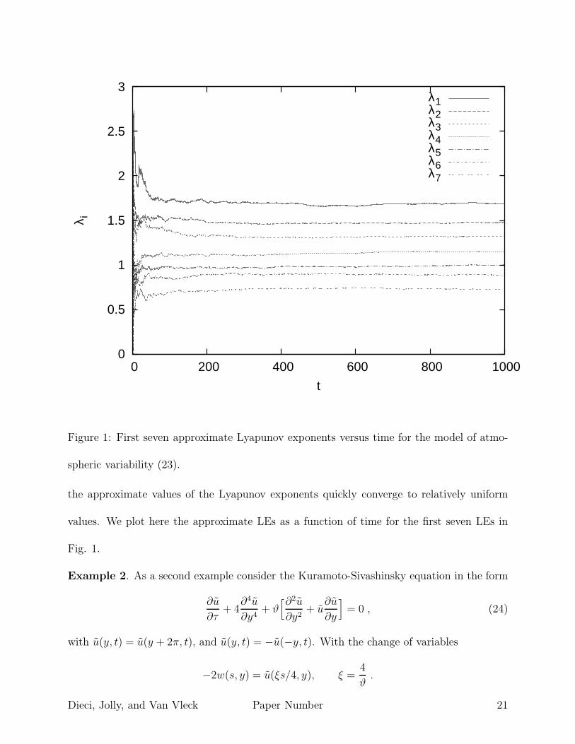
Example 1. The first example is a model of atmospheric variability [27, 28] with values xj
of m points equally spaced around a circle of constant latitude:
xk = (xk+1 − xk−2)xk−1 − xk + 8 , k = 0, 1, . . . , m − 1 , (mod m) . (23)
In the results reported in [27, 28] for m = 40 there are 13 positive LEs, the Kaplan-Yorke
dimension dimKY ≈ 27, and λ14 = 0. As a concrete example we considered the initial
condition x(0) = e2, the second unit basis vector, and solved for all LEs using LESNLS and
LESNLL. We employed error tolerances on the trajectory, orthogonal factor, and Lyapunov
exponents of size 10−4 and the RK38 scheme. Over integration times up to 104 we found
the computational procedure for large problems LESNLL to be approximately twice as
fast as that for small problems LESNLS when computing all Lyapunov exponents. In
addition, we obtained values of the Kaplan-Yorke dimension dimKY ≈ 27.06 and found that
Dieci, Jolly, and Van Vleck Paper Number 20
0
0.5
1
1.5
2
2.5
3
0 200 400 600 800 1000
λ i
t
λ1λ2λ3λ4λ5λ6λ7
Figure 1: First seven approximate Lyapunov exponents versus time for the model of atmo-
spheric variability (23).
the approximate values of the Lyapunov exponents quickly converge to relatively uniform
values. We plot here the approximate LEs as a function of time for the first seven LEs in
Fig. 1.
Example 2. As a second example consider the Kuramoto-Sivashinsky equation in the form
∂u
∂τ+ 4
∂4u
∂y4+ ϑ
[∂2u
∂y2+ u
∂u
∂y
]
= 0 , (24)
with u(y, t) = u(y + 2π, t), and u(y, t) = −u(−y, t). With the change of variables
−2w(s, y) = u(ξs/4, y), ξ =4
ϑ.
Dieci, Jolly, and Van Vleck Paper Number 21
(24) can be written as
ws = (w2)y − wyy − ξwyyyy . (25)
This allows us to compare to the Lyapunov exponents reported in [11] and [13]. All computa-
tions were performed for ξ = 0.02991, ϑ = 133.73454, one of the parameter values considered
in [11, 13, 39].
We consider a spatial discretization using standard Galerkin truncation with 16 or 32
modes (see [13] for more details). We employ LESNLL using the DP integrator for both the
discrete (Table 1) and the continuous QR (Table 2) and the three step strategy (Table 3)
using LESLIL (with the DP integrator and the continuous QR method) and the stiff solver
VODPK [6] to approximate the solution of (1).
We report on numerical experiments to solve for the first four Lyapunov exponents over
intervals of length 10 and 100. In Table 1-3, T denote the final time, M the number of
modes, N the number of exponents approximated, and TOL is the value of the tolerances
that were employed. We report on the approximate Lyapunov exponents obtained and record
normalized CPU times. The values of the LEs obtained are consistent across the different
methods and with previous results [11, 13]. For M=16 modes, the discrete and continuous
QR approach take essentially the same amount of CPU time, and are considerably faster
than the three step strategy. For M=32, the discrete QR method is faster than all others.
DISCUSSION
We have developed a toolbox for approximation of Lyapunov exponents for nonlinear dif-
ferential equations. Among the benefits of the techniques described is the ability to use
Dieci, Jolly, and Van Vleck Paper Number 22
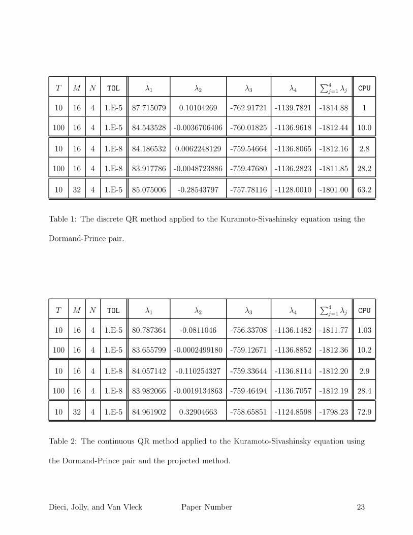
T M N TOL λ1 λ2 λ3 λ4
∑4j=1 λj CPU
10 16 4 1.E-5 87.715079 0.10104269 -762.91721 -1139.7821 -1814.88 1
100 16 4 1.E-5 84.543528 -0.0036706406 -760.01825 -1136.9618 -1812.44 10.0
10 16 4 1.E-8 84.186532 0.0062248129 -759.54664 -1136.8065 -1812.16 2.8
100 16 4 1.E-8 83.917786 -0.0048723886 -759.47680 -1136.2823 -1811.85 28.2
10 32 4 1.E-5 85.075006 -0.28543797 -757.78116 -1128.0010 -1801.00 63.2
Table 1: The discrete QR method applied to the Kuramoto-Sivashinsky equation using the
Dormand-Prince pair.
T M N TOL λ1 λ2 λ3 λ4
∑4j=1 λj CPU
10 16 4 1.E-5 80.787364 -0.0811046 -756.33708 -1136.1482 -1811.77 1.03
100 16 4 1.E-5 83.655799 -0.0002499180 -759.12671 -1136.8852 -1812.36 10.2
10 16 4 1.E-8 84.057142 -0.110254327 -759.33644 -1136.8114 -1812.20 2.9
100 16 4 1.E-8 83.982066 -0.0019134863 -759.46494 -1136.7057 -1812.19 28.4
10 32 4 1.E-5 84.961902 0.32904663 -758.65851 -1124.8598 -1798.23 72.9
Table 2: The continuous QR method applied to the Kuramoto-Sivashinsky equation using
the Dormand-Prince pair and the projected method.
Dieci, Jolly, and Van Vleck Paper Number 23
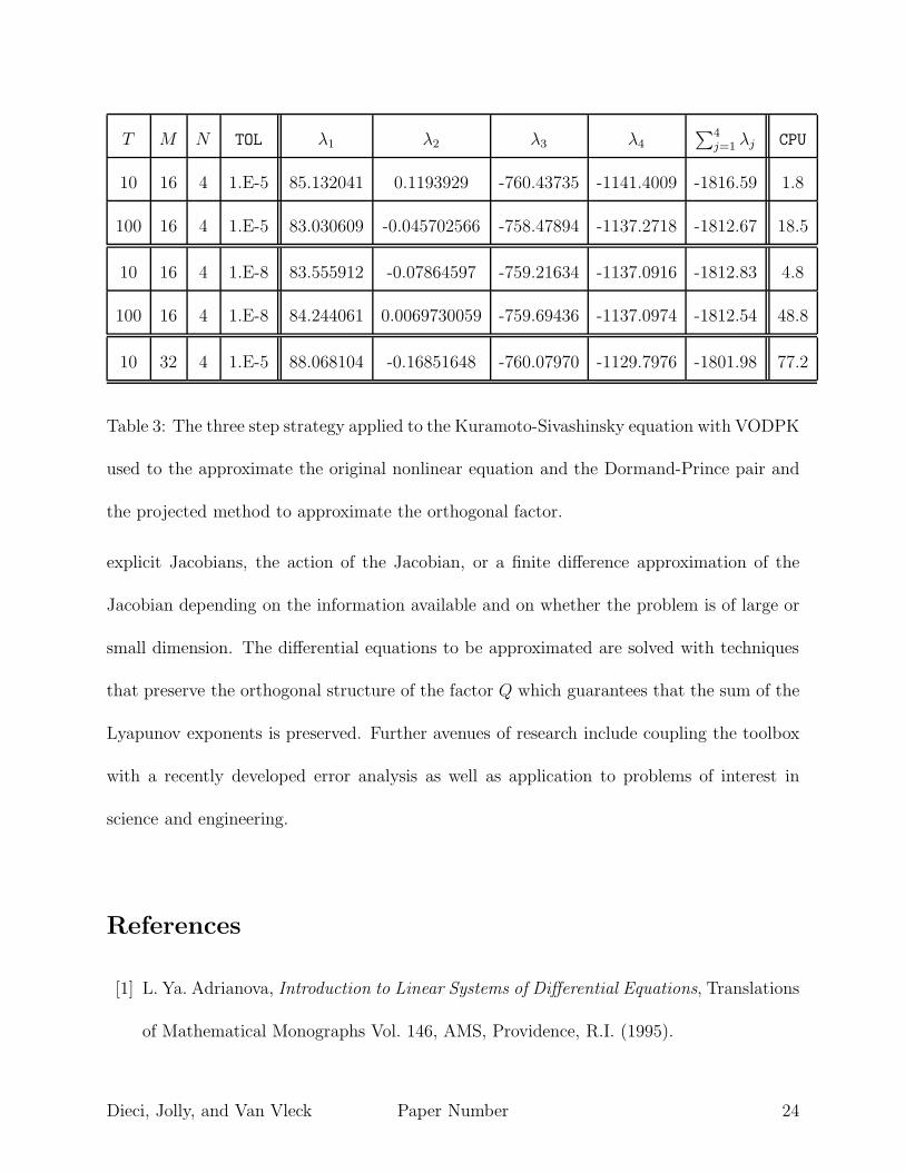
T M N TOL λ1 λ2 λ3 λ4
∑4j=1 λj CPU
10 16 4 1.E-5 85.132041 0.1193929 -760.43735 -1141.4009 -1816.59 1.8
100 16 4 1.E-5 83.030609 -0.045702566 -758.47894 -1137.2718 -1812.67 18.5
10 16 4 1.E-8 83.555912 -0.07864597 -759.21634 -1137.0916 -1812.83 4.8
100 16 4 1.E-8 84.244061 0.0069730059 -759.69436 -1137.0974 -1812.54 48.8
10 32 4 1.E-5 88.068104 -0.16851648 -760.07970 -1129.7976 -1801.98 77.2
Table 3: The three step strategy applied to the Kuramoto-Sivashinsky equation with VODPK
used to the approximate the original nonlinear equation and the Dormand-Prince pair and
the projected method to approximate the orthogonal factor.
explicit Jacobians, the action of the Jacobian, or a finite difference approximation of the
Jacobian depending on the information available and on whether the problem is of large or
small dimension. The differential equations to be approximated are solved with techniques
that preserve the orthogonal structure of the factor Q which guarantees that the sum of the
Lyapunov exponents is preserved. Further avenues of research include coupling the toolbox
with a recently developed error analysis as well as application to problems of interest in
science and engineering.
References
[1] L. Ya. Adrianova, Introduction to Linear Systems of Differential Equations, Translations
of Mathematical Monographs Vol. 146, AMS, Providence, R.I. (1995).
Dieci, Jolly, and Van Vleck Paper Number 24
[2] D. Arasteh, “Measures of Order in Dynamic Systems”, J. Comput. Nonlinear Dynam.
3 (2008), 031002.
[3] O. Bendiksen, “Localization phenomena in structural dynamics”, Chaos, Solitons &
Fractals 11-10 (2000), pp. 1621–1660.
[4] G. Benettin, L. Galgani, A. Giorgilli and J.-M. Strelcyn, “Lyapunov Exponents for
Smooth Dynamical Systems and for Hamiltonian Systems; A Method for Computing
All of Them. Part 1: Theory ”, and “ . . . Part 2: Numerical Applications ”, Meccanica
15 (1980), pp. 9–20, 21–30.
[5] P. Blomgren, A. Palacios, B. Zhu, S. Daw, C. Finney, J. Halow and S. Pannala, “Bifur-
cation analysis of bubble dynamics in fluidized beds”, CHAOS 17 (2007), 013130.
[6] P. Brown and A. Hindmarsh, “Matrix free methods for stiff systems of ODEs”, SIAM
J. Numer. Anal. 23 (1986), pp. 610–638.
[7] B.F. Bylov and N.A. Izobov, “Necessary and sufficient conditions for stability of charac-
teristic exponents of a linear system”, Differentsial’nye Uravneniya 5 (1969), pp. 1794–
1903.
[8] M. P. Calvo, A. Iserles, and A. Zanna, “Numerical solution of isospectral flows”, Math.
Comp. 66 (1997), pp. 1461–1486.
[9] M.T. Chu, “On the continuous realization of iterative processes”, SIAM Review 30
(1988), pp. 375–387.
Dieci, Jolly, and Van Vleck Paper Number 25
[10] P. Constantin and C. Foias, “Global Lyapunov exponents, Kaplan-Yorke formulas and
the dimension of the attractors for 2D Navier-Stokes equations”, Comm. Pure Appl.
Math. 38 (1985), pp. 1–27.
[11] F. Christiansen, P. Cvitanovic, and V. Putkaradze, “Spatiotemporal chaos in terms of
unstable recurrent patterns”, Nonlinearity, 10 (1997), pp. 55–70.
[12] L. Dai, “Implementation of Periodicity Ratio in Analyzing Nonlinear Dynamic Systems:
A Comparison With Lyapunov Exponent”, J. Comput. Nonlinear Dynam. 3 (2008),
011006.
[13] L. Dieci, M. S. Jolly, M. S., R. Rosa, E. S. Van Vleck, “Error in approximation of Lya-
punov exponents on inertial manifolds: the Kuramoto-Sivashinsky equation”, Discrete
Contin. Dyn. Syst. Ser. B 9 (2008), pp. 555–580.
[14] L. Dieci, R. D. Russell, and E. S. Van Vleck. On the computation of Lyapunov exponents
for continuous dynamical systems. SIAM J. Numer. Anal., 34:402–423, 1997.
[15] L. Dieci and E. S. Van Vleck. Computation of a few Lyapunov exponents for continuous
and discrete dynamical systems. Applied Numerical Math., 17:275–291, 1995.
[16] L. Dieci and E. S. Van Vleck, “Computation of orthonormal factors for fundamental
solution matrices”, Numer. Math. 83 (1999), pp. 599–620.
[17] L. Dieci and E. S. Van Vleck, “Lyapunov and other spectra: a survey”, In D. Estep and
S. Tavener, editors, Preservation of Stability under Discretization. SIAM, Philadelphia,
2002.
Dieci, Jolly, and Van Vleck Paper Number 26
[18] L. Dieci, E. S. Van Vleck, “Lyapunov spectral intervals: theory and computation”,
SIAM J. Numer. Anal. 40 (2002), pp. 516–542.
[19] L. Dieci, E. S. Van Vleck, “On the error in computing Lyapunov exponents by QR
methods”, Numer. Math. 101 (2005), pp. 619–642.
[20] L. Dieci, E. S. Van Vleck, “Perturbation theory for approximation of Lyapunov expo-
nents by QR methods”, J. Dynam. Differential Equations 18 (2006), pp. 815–840.
[21] L. Dieci, E. S. Van Vleck, “Lyapunov and Sacker-Sell spectral intervals”, J. Dynam.
Differential Equations 19 (2007), pp. 265–293.
[22] L. Dieci, E. S. Van Vleck, “On the error in QR integration”, SIAM J. Numer. Anal. 46
(2008), pp. 1166–1189.
[23] L. Dieci and E. S. Van Vleck. “LESLIS and LESLIL: Codes
For Approximating Lyapunov Exponents of linear systems”, See:
http://www.math.gatech.edu/∼dieci/software-les.html
[24] S.P. Diliberto, “On Systems of Ordinary Differential Equations,” in Contributions to the
Theory of Nonlinear Oscillations (Ann. of Math. Studies 20), Princeton Univ. Press,
Princeton (1950), pp. 1–38.
[25] E. Elnashaie and J. Grace, “Complexity, bifurcation and chaos in natural and man-
made lumped and distributed systems”, Chemical Engineering Science 62-13 (2007),
pp. 3295–3325.
Dieci, Jolly, and Van Vleck Paper Number 27
[26] E. Hairer, S. P. Nœrsett, and G. Wanner, Solving Ordinary Differential Equations I.
Springer-Verlag, Berlin-Heidelberg, (1993) Second edition.
[27] E. Lorenz, “Predictability. A problem partly solved”, in Proceedings on predictability
held at ECMWF on 4-8 September 1995, pp. 1-18. [Available from ECMWF, Shinfield
Park, Reading, Berkshire RG29AX, [email protected]] (1996), pp. 1–18.
[28] E. Lorenz and K. Emmanuel, “Optimal sites for supplementary weather observations:
Simulations with a small model”, J. Atmos. Sci. 55 (1998), pp. 399–414.
[29] A. Lyapunov, “Problem general de la stabilite du mouvement”, Int. J. Control 53
(1992), pp. 531–773.
[30] V. M. Millionshchikov. Structurally stable properties of linear systems of differential
equations. Differents. Uravneniya, 5:1775–1784, 1969.
[31] V. M. Millionshchikov. Systems with integral division are everywhere dense in the set of
all linear systems of differential equations. Differents. Uravneniya, 5:1167–1170, 1969.
[32] V. I. Oseledec, “A multiplicative ergodic theorem. Lyapunov characteristic numbers for
dynamical systems”, Trans. Moscow Mathem. Society 19 (1998), 197.
[33] E. Ott, Chaos in dynamical systems. Cambridge University Press, New York, (1993).
[34] K. J. Palmer, “The structurally stable systems on the half-line are those with exponen-
tial dichotomy,” J. Diff. Eqn. 33 (1979), pp. 16–25.
[35] K. J. Palmer, “Exponential dichotomy, integral separation and diagonalizability of linear
sys temsof ordinary differential equations,” J. Diff. Eqn. 43 (1982), pp. 184–203.
Dieci, Jolly, and Van Vleck Paper Number 28
[36] K. J. Palmer,“Exponential separation, exponential dichotomy and spectral theory for
linear s ystems of ordinary differential equations,” J. Diff. Eqn. 46 (1982), pp. 324–345.
[37] O. Perron, “Die Ordnungszahlen Linearer Differentialgleichungssystemen,” Math. Zeits.
31 (1930), pp. 748–766.
[38] D. Ruelle, Chaotic evolution and strange attractors. Cambridge University Press, Cam-
bridge, (1989).
[39] Y. S. Smyrlis and D. T. Papageorgiou, Predicting chaos for infinite-dimensional dy-
namical systems: the Kuramoto-Sivashinsky equation, a case study, Proc. Nat. Acad.
Sci. U.S.A., 88 (1991), pp. 11129–11132.
[40] E. S. Van Vleck, “On the Error in the Product QR Decomposition”, to appear in SIAM
J. Matr. Anal. Applic., (2010).
[41] A. Wolf, J. B. Swift, H. L. Swinney and J. A. Vastano, “Determining Lyapunov Expo-
nents from a Time Series, ” Physica D 16 (1985), pp. 285–317.
[42] M. Xu and Z. Gao, “Nonlinear Analysis of Road Traffic Flows in Discrete Dynamical
System”, J. Comput. Nonlinear Dynam. 3 (2008), 021206.
Dieci, Jolly, and Van Vleck Paper Number 29