Seediscussions,stats,andauthorprofilesforthispublicationat:https://www.researchgate.net/publication/309242704

NumericalsolutiontoalinearizedtimefractionalKdVequationonunboundeddomains

ArticleinMathematicsofComputation·January2016

DOI:10.1090/mcom/3229

CITATIONS

0

READS

64

4authors,including:

Someoftheauthorsofthispublicationarealsoworkingontheserelatedprojects:

NumericalmethodsfortimeandspacefractionalpartialdifferentialequationsViewproject

QianZhang

BeijingComputationalScienceResearchCen…

2PUBLICATIONS3CITATIONS

SEEPROFILE

JiweiZhang

BeijingComputationalScienceResearchCen…

30PUBLICATIONS166CITATIONS

SEEPROFILE

ZhiminZhang

WayneStateUniversity

21PUBLICATIONS90CITATIONS

SEEPROFILE

AllcontentfollowingthispagewasuploadedbyQianZhangon17November2016.

Theuserhasrequestedenhancementofthedownloadedfile.Allin-textreferencesunderlinedinblueareaddedtotheoriginaldocument

andarelinkedtopublicationsonResearchGate,lettingyouaccessandreadthemimmediately.

MATHEMATICS OF COMPUTATIONVolume 00, Number 0, Pages 000–000S 0025-5718(XX)0000-0

NUMERICAL SOLUTION TO A LINEARIZED TIME

FRACTIONAL KDV EQUATION ON UNBOUNDED DOMAINS

QIAN ZHANG, JIWEI ZHANG, SHIDONG JIANG, AND ZHIMIN ZHANG

Abstract. An efficient numerical scheme is developed to solve a linearizedtime fractional KdV equation on unbounded spatial domains. First, the exactabsorbing boundary conditions (ABCs) are derived which reduces the pureinitial value problem into an equivalent initial-boundary value problem on afinite interval that contains the compact support of the initial data and theinhomogeneous term. Second, the stability of the reduced initial-boundaryvalue problem is studied in detail. Third, an efficient unconditionally sta-ble finite difference scheme is constructed to solve the initial-boundary valueproblem where the nonlocal fractional derivative is evaluated via a sum-of-exponentials approximation for the convolution kernel. As compared with thedirect method, the resulting algorithm reduces the storage requirement fromO(MN) to O(M logd N) and the overall computational cost from O(MN2)

to O(MN logd N) with M the total number of spatial grid points and N thetotal number of time steps. Here d = 1 if the final time T is much greaterthan 1 and d = 2 if T ≈ 1. Numerical examples are given to demonstrate theperformance of the proposed numerical method.

1. Introduction

The classical Korteweg-de Vries (KdV) equation is a typical dispersive nonlinearpartial differential equation (PDE). Historically, the solitary solution of the equa-tion was first observed physically by Scott Russell in 1834 [27], and the equationitself was later derived by Korteweg and de Vries in 1895 [19]. Since then, it hasbeen applied in many fields to describe a wide range of physical phenomena suchas interaction of nonlinear waves [33], collision-free hydro-magnetic waves in a coldplasma, ion-acoustic waves, interfacial electrohydrodynamics [9], etc. As a mathe-matical model of the water wave, when the wave height is small compared to thewater depth [32], the nonlinear equation is reduced to the linear KdV equation.

When these physical phenomena are considered non-conservative, they can bedescribed using fractional differential equations. Over the last two decades thefractional calculus has been applied to almost every field of science, engineering,and mathematics [18, 20, 22, 24, 25]. Here we consider pure initial value problem

2010 Mathematics Subject Classification. 33F05, 35Q40, 35Q55, 34A08, 35R11, 26A33.The research of this author was supported in part by the National Natural Science Foundation

of China under grants 91430216 and U1530401.The research of this author was supported in part by NSF under grant DMS-1418918.The research of this author was supported in part by the National Natural Science Foundation

of China under grants 11471031, 91430216, and by NSF under grant DMS-1419040.

c©XXXX American Mathematical Society

1

2 Q. ZHANG, J. ZHANG, S. JIANG, AND Z. ZHANG

(IVP) of the linearized time-fractional KdV equation in one space dimension:

(1.1)

C0D

αt u(x, t) + uxxx(x, t) = f(x, t), t ∈ (0, T ], x ∈ R,

u(x, 0) = u0(x), x ∈ R,

u(x, t) → 0, when |x| → ∞, t ∈ (0, T ],

where the source term f(x, t) and initial value u0(x) are assumed to be compactlysupported, and the operator C

0Dαt (0 < α < 1) stands for the Caputo fractional

derivative and is defined by the formula

(1.2) C0D

αt u(x, t) =

1

Γ(1− α)

∫ t

0

u′(x, s)

(t− s)αds.

Although there are some methods to analytically solve the fractional KdV equa-tion in some special cases [8, 23, 31, 35], one may have to resort to the numericalmethods to obtain its solution in general. There are two difficulties when one triesto solve (1.1) numerically. First, the original problem is defined on the whole spatialdomain, which has to be truncated to a finite domain for the purpose of numericalcomputation. For this, one needs to impose some artificial boundary conditionsat the boundary of the truncated domain. These boundary conditions have to becarefully chosen so that there will be no reflections from the boundary and thereduced initial-boundary value problem (IBVP) is still stable and equals to theoriginal problem in the truncated domain. Second, the fractional derivative is de-fined as a convolution integral from 0 to the current time t, and a direct method ofevaluating the fractional derivative requires the storage of the solution at all timesand quadratic complexity in computational cost, which is prohibitively expensivefor large-scale long-time simulations.

Among these artificial boundary conditions, the so-called exact absorbing bound-ary conditions (ABCs) prevent the reflections of the wave from the boundary, whichleads to an equivalent IBVP formulation for the original IVP. For the linearized KdVequation of the integer order, Zheng, Han, and Wen [37] derived the exact ABCsvia the Laplace transform. Recently, Zhang, Li, and Wu [34] developed a seriesof high-order local ABCs to approximate the exact ABCs using Pade expansion inthe Laplace domain. Besse et al. [5] constructed the discrete ABCs for the fullydiscrete problem using the Z-transformation.

In this paper, we first derive exact ABCs for the linearized fractional KdV equa-tion (1.1) with standard techniques in this field. That is, we apply the Laplacetransform in time to reduce the equation to an ODE; we then use the conditionthat the solution has to decay to zero at infinity to obtain the solution of the ODEin the left and right exterior domains, which also leads to boundary conditions attwo end points in the Laplace domain; the boundary conditions in the physicalspace are obtained by inverting back. However, unlike many second order differ-ential equations where only one boundary condition at each end point is needed,the KdV equation involves third order derivatives in space and one more boundarycondition is required. All three absorbing boundary conditions are carefully chosenand we then show that the IBVP with our exact ABCs is stable in the L2 norm.

Next, we construct a delicate finite difference (FD) scheme to discretize the IBVP.Our construction starts from the introduction of an auxillary variable which reducesthe third-order PDE to a second-order one. We then combine the PDE and theexact ABCs to obtain more consistent discrete equations for the boundary points.

NUMERICAL SOLUTION TO A LTF KDV EQUATION ON UNBOUNDED DOMAINS 3

This way, we are able to show that the resulting FD scheme is unconditionallystable; whereas the naive FD schemes which discretize the spatial derivatives viacentral difference for interior points and one-sided differences for boundary pointsis only conditionally stable.

We further apply the fast algorithm in [15] to reduce the computational andstorage cost for the evaluation of the fractional derivatives in the temporal vari-able. Here the main idea is to approximate the convolution kernel t−1−α (obtainedby integration by parts for the integral on the right hand side of (1.2)) by a sum-of-exponentials (SOE) approximation when t is away from the origin. For eachspatial point, the convolution with the exponential kernel can be evaluated in O(1)time at each time step via standard recurrence relation or any A-stable ODE solver(see, for example, [2–4,6,12–15,21,36]). This reduces the computational cost fromO(N2) for direct method to O(NNexp) and the storage cost from O(N) for directmethod to O(Nexp), where N is the total number of time steps and Nexp is thetotal number of the exponentials needed in the SOE approximation. When similarSOE approximations are used for the exact ABCs as well, the overall computa-tional cost of our algorithm is O(MNNexp) as compared with O(MN2) for directmethod; and the storage requirement of our algorithm is O(MNexp) as comparedwith O(MN) for direct method, as the direct method needs to store the solution inthe whole computational spatial domain at all times. Here M is the total numberof discretization points in space. The number of exponentials Nexp needed in theSOE approximation depends on the prescribed precision ε, the cut-off time stepsize δ, and the final time T . For a fixed absolute precision, Nexp = O(logN) when

T ≫ 1 and Nexp = O(log2 N) when T ≈ 1 if we assume that N = Tδ , i.e., a uniform

mesh is used in the temporal variable and the time step size is chosen to be ∆t = δ.The rest of the paper is organized as follows. In Section 2, we derive the exact

ABCs for the linearized fractional KdV equation. In Section 3, we present thestability analysis of the reduced IBVP. In Section 4, we develop an efficient andstable finite difference scheme for solving the IBVP. Some numerical examples aregiven to demonstrate the performance of our scheme in Section 5. Finally, weconclude our paper with a short summary.

2. The derivation of exact ABCs

We use the artificial boundary methods (ABMs) [11, 30] to construct the exactABCs. We first introduce artificial boundaries Γl := x|x = xl and Γr := x|x =xr to divide the original infinite domain into three parts: the computational do-main of interest Ωc := (xl, xr), the left unbounded exterior domain Ωl := (−∞, xl),and the right unbounded exterior domain Ωr := (xr ,∞). The choices of parametersxl and xr are determined such that the initial data u0(x) and the source term fare compactly supported in Ωc. We consider the following two exterior problemson Ωl := (−∞, xl) and Ωr := (xr,∞), respectively.

C0D

αt u(x, t) + uxxx(x, t) = 0, t ∈ (0, T ], x ∈ Ωr,(2.1)

u(x, 0) = 0, x ∈ Ωr,(2.2)

u(x, t) → 0, when x → +∞, t ∈ (0, T ],(2.3)

and

C0D

αt u(x, t) + uxxx(x, t) = 0, t ∈ (0, T ], x ∈ Ωl,(2.4)

4 Q. ZHANG, J. ZHANG, S. JIANG, AND Z. ZHANG

u(x, 0) = 0, x ∈ Ωl,(2.5)

u(x, t) → 0, when x → −∞, t ∈ (0, T ].(2.6)

We now derive certain conditions that must be satisfied for the solution u at theartificial boundaries xl and xr.

Let u(x, s) be the Laplace transform of u(x, t) defined by

u(x, s) =

∫ +∞

0

e−stu(x, t)dt, ℜ(s) > 0.

The Laplace transform of the Caputo derivatives is given by the formula

C0D

αt u(x, s) = sαu(x, s)− sα−1u(x, 0), 0 < α ≤ 1.

Applying the Laplace transform on equations (2.1) and (2.4) with zero initial values(2.2) and (2.5), we obtain an ODE in u(x, s)

(2.7) sαu(x, s) + uxxx(x, s) = 0, x ∈ Ωl ∪ Ωr.

The general solution of (2.7) is given by the formula

(2.8) u(x, s) = c1(s)eλ1(s)x + c2(s)e

λ2(s)x + c3(s)eλ3(s)x,

where λ1(s), λ2(s), λ3(s) are the roots of the cubic equation

sα + λ3 = 0.

That is,

λ1(s) = −sα

3 , λ2(s) = −sα

3 ω, λ3(s) = −sα

3 ω2(2.9)

with w = e2πi/3. It is easy to see that ℜ(λ1(s)) < 0, ℜ(λ2(s)) > 0, ℜ(λ3(s)) > 0.Applying the Laplace transform on (2.3) and (2.6), we have

(2.10) u(x, s) → 0, when |x| → ∞.

Thus, on the interval Ωr,

u(x, s) = c1(s)eλ1(s)x.

Taking derivatives of this solution with respect to x, we obtain

uxx(x, s) = λ21(s)u(x, s) and ux(x, s) = λ1(s)u(x, s),(2.11)

or equivalently

1

λ21(s)

uxx(x, s) = u(x, s) and1

λ1(s)ux(x, s) = u(x, s).(2.12)

Applying the inverse Laplace transform (see [25]) to (2.11) and (2.12) yields

uxx(x, t) =C0D

2α3

t u(x, t) and ux(x, t) = −C0D

α

3

t u(x, t),(2.13)

I2α3

t uxx(x, t) = u(x, t) and Iα

3

t ux(x, t) = −u(x, t),(2.14)

where Iαt with α > 0 is the Riemann-Liouville factional integral defined by the

formula

(2.15) Iαt g(t) =

1

Γ(α)

∫ t

0

g(τ)

(t− τ)1−αdτ, t > 0.

Similarly, on the interval Ωl, we have c1 = 0 from the decay condition (2.8) asx → −∞. Hence, the solution is

u(x, s) = c2(s)eλ2(s)x + c3(s)e

λ3(s)x.

NUMERICAL SOLUTION TO A LTF KDV EQUATION ON UNBOUNDED DOMAINS 5

Taking first and second derivatives of u and eliminating c2 and c3, we obtain

uxx(x, s)− (λ2 + λ3)ux(x, s) + λ2λ3u(x, s) = 0.

Using the facts that λ2 + λ3 = −λ1 and λ2λ3 = λ21, we have

(2.16) u(x, s) +1

λ1(s)ux(x, s) +

1

λ21(s)

uxx(x, s) = 0,

or equivalently,

(2.17) λ21(s)u(x, s) + λ1(s)ux(x, s) + uxx(x, s) = 0.

Applying the inverse Laplace transform to (2.16) and (2.17) leads to

u(x, t)− Iα

3

t ux(x, t) + I2α3

t uxx(x, t) = 0,(2.18)

uxx(x, t)−C0D

α

3

t ux(x, t) +C0D

2α3

t u(x, t) = 0.(2.19)

Using (2.14) and (2.18) as exact artificial boundary conditions, the original IVP(1.1) is reduced to the the following IBVP on Ωc:

C0D

αt u(x, t) + uxxx(x, t) = f(x, t), x ∈ Ωc, t ∈ (0, T ],(2.20)

u(x, 0) = u0(x), x ∈ Ωc,(2.21)

I2α3

t uxx(xr, t) = u(xr, t),(2.22)

Iα

3

t ux(xr , t) = −u(xr, t),(2.23)

I2α3

t uxx(xl, t)− Iα

3

t ux(xl, t) + u(xl, t) = 0.(2.24)

Similarly, using (2.13) and (2.19) as exact artificial boundary conditions, the origi-nal IVP (1.1) is reduced to the following IBVP on Ωc:

C0D

αt u(x, t) + uxxx(x, t) = f(x, t), x ∈ Ωc, t ∈ (0, T ],(2.25)

u(x, 0) = u0(x), x ∈ Ωc,(2.26)

uxx(xr , t) =C0D

2α3

t u(xr, t),(2.27)

ux(xr, t) = −C0D

α

3

t u(xr, t),(2.28)

uxx(xl, t)−C0D

α

3

t ux(xl, t) +C0D

2α3

t u(xl, t) = 0.(2.29)

3. Stability of the exact absorbing boundary conditions

We now show that both the IBVP (2.20)–(2.24) and the IBVP (2.25)–(2.29) arestable in L2 norm. We begin with some useful lemmas.

Lemma 3.1 (see [1]). Suppose that v(t) is absolutely continuous on [0,T]. Then

v(t)C0Dαt v(t) ≥

1

2C0D

αt v

2(t), 0 < α < 1.

Lemma 3.2 (see [25]). Suppose that v(t) satisfies the inequality

v(t) ≤ a(t) + b(t)

∫ t

0

(t− s)α−1v(s)ds, α > 0,

for t ∈ [0, T ], where a(t) is not decreasing, nonnegative and locally integrable over[0,T], and b(t) is nonnegative and nondecreasing. Then

v(t) ≤ a(t)Eα(b(t)Γ(α)tα), 0 ≤ t ≤ T,

6 Q. ZHANG, J. ZHANG, S. JIANG, AND Z. ZHANG

where Eα(z) =∑∞

n=0zn

Γ(nα+1) is the Mittag-Leffler function.

Lemma 3.3. Suppose that y(t) is absolutely continuous on [0,T]. Then

I1tC0D

αt y(t) = −

t1−α

Γ(2− α)y(0) + I1−α

t y(t).

Proof. Using the definitions for the Caputo fractional derivative (1.2) and Riemann-Liouville integral (2.15), we obtain

I1tC0D

αt y(t) =

∫ t

0

1

Γ(1− α)

∫ τ

0

y′(η)

(τ − η)αdηdτ.

Exchanging the order of integration and performing integration by parts, we have

I1tC0D

αt y(t) =

1

Γ(1− α)

∫ t

0

y′(η)

∫ t

η

1

(τ − η)αdτdη

=1

Γ(1− α)(1 − α)

∫ t

0

y′(η)(t− η)1−αdη

= −t1−α

Γ(2− α)y(0) +

1

Γ(1− α)

∫ t

0

y(η)

(t− η)αdη

= −t1−α

Γ(2− α)y(0) + I1−α

t y(t),

and the proof is complete.

Lemma 3.4. For any T > 0, suppose f and g are smooth functions with f(0) =g(0) = 0. Then

I1t (2fI

23α

t f − (Iα

3

t f)2)|t=T ≥ 0,(3.1)

I1t (2(I

α

3

t g − I23α

t f)f − g2)|t=T ≤ 0.(3.2)

Proof. For any T > 0, we set F (t) = f(t)1[0,T ], G(t) = g(t)1[0,T ](t), where 1[0,T ](t)

is the characteristic function of [0, T ]. We may then extend the integration domainas follows:

I1t (2fI

23α

t f − (Iα

3

t f)2)|t=T = I1t (2FI

23α

t F − (Iα

3

t F )2)|t=T

=

∫ +∞

0

(2FI23α

t F − (Iα

3

t F )2)dt.

We now employ the Plancherel theorem to obtain∫ +∞

0

(2FI23α

t F − (Iα

3

t F )2)dt

=1

2π

∫ +∞

−∞

(2(iξ)−23α − |ξ|

− 23α)∣

∣

∣F (iξ)

∣

∣

∣

2

dξ

=1

2π

∫ +∞

0

[

(2(iξ)−23α − |ξ|

− 23α) + (2(−iξ)−

23α − |ξ|

− 23α)] ∣

∣

∣F (iξ)

∣

∣

∣

2

dξ

=1

2π

∫ +∞

0

2(2 cosπα

3− 1) |ξ|−

2α3

∣

∣

∣F (iξ)

∣

∣

∣

2

dξ

≥ 0,

NUMERICAL SOLUTION TO A LTF KDV EQUATION ON UNBOUNDED DOMAINS 7

where we have used the fact that 1 < 2 cos πα3 < 2 for 0 < α < 1 and (3.1) is

proved. In addition, we have

I1t (2(I

α

3

t g − I23α

t f)f − g2)|t=T

=

∫ +∞

0

[

2(Iα

3

t G− I23α

t F )F −G2]

dt

≤

∫ +∞

0

[

2FIα

3

t G− (Iα

3

t F )2 −G2]

dt

=1

2π

∫ +∞

−∞

(

2(iξ)−α

3 G(iξ)¯F (iξ)− |ξ|

− 2α3

∣

∣

∣F (iξ)

∣

∣

∣

2

−∣

∣

∣G(iξ)

∣

∣

∣

2)

dξ

≤ −1

2π

∫ +∞

−∞

(

∣

∣

∣G(iξ)

∣

∣

∣− |ξ|

−α

3

∣

∣

∣F (iξ)

∣

∣

∣

)2

dξ

≤ 0.

Here the first inequality follows from (3.1) and the second equality follows from thePlancherel theorem again.

Theorem 3.5. The IBVP (2.20)–(2.24) is L2-stable. More precisely, for 0 < t ≤T , the following estimate holds

∫ t

0

‖u(·, τ)‖2dτ ≤ Iα

t

( t1−α

Γ(2− α)Eα(t

α))

‖u(·, 0)‖2

(3.3)

+ Iαt

(

Eα(tα)

∫ t

0

‖f(·, τ)‖2dτ)

.

Proof. Multiplying both sides of (2.20) with 2u, integrating x from xl to xr, andapplying integration by parts, we obtain

2

∫ xr

xl

u C0D

αt udx = −2

∫ xr

xl

(uuxx −1

2u2x)xdx+

∫ xr

xl

2ufdx(3.4)

= (2uuxx − u2x)(xl, t)− (2uuxx − u2

x)(xr , t) +

∫ xr

xl

2ufdx.

The exact ABCs (2.22)-(2.24) can be rewritten as follows:

u(xr, t) = −I2α3

t uxx(xr , t), ux(xr , t) = Iα

3

t uxx(xr, t),

u(xl, t) = −I2α3

t uxx(xl, t) + Iα

3

t ux(xl, t),

where the second equality follows from the differentiation of (2.23). Replacingu(xl, t), u(xr, t) and ux(xr, t) in (3.4) by the above integrals, we have

2

∫ xr

xl

u C0D

αt udx =

[

2(Iα

3

t ux − I23α

t uxx)uxx − u2x

]

(xl, t)

−[

2uxxI23α

t uxx − (Iα

3

t uxx)2]

(xr, t) + 2

∫ xr

xl

fudxdτ.

Integrating both sides of the above equation over [0, t] and then applying the lemmas3.1 and 3.4, we obtain

I1tC0D

αt

∫ xr

xl

u2dx ≤ 2

∫ t

0

∫ xr

xl

fudxdτ.

8 Q. ZHANG, J. ZHANG, S. JIANG, AND Z. ZHANG

The applications of the Lemma 3.3 and the Cauchy-Schwartz inequality yield

I1−αt

∫ xr

xl

u2dx ≤t1−α

Γ(2− α)

∫ xr

xl

u(x, 0)2dx(3.5)

+

∫ t

0

∫ xr

xl

u2dxdτ +

∫ t

0

∫ xr

xl

f2dxdτ.(3.6)

Let v(t) := I1−αt

(

∫ xr

xl

u2dx)

and a(t) := t1−α

Γ(2−α)

∫ xr

xl

u20(x)dx+

∫ t

0

∫ xr

xl

f2(x, t)dxdτ .

Using the property of the Riemann-Liouville integral Iαt (I

βt )g(t) = Iα+β

t g(t) for

α, β ∈ R+, we may rewrite∫ t

0

∫ xr

xl

u2dxdτ as follows:

∫ t

0

∫ xr

xl

u2dxdτ = I1t

∫ xr

xl

u2dx = Iαt (I

1−αt

∫ xr

xl

u2dx) = Iαt v(t).

Hence, (3.5) can be rewritten as follows:

v(t) ≤ a(t) + Iαt v(t) = a(t) +

1

Γ(α)

∫ t

0

(t− τ)α−1v(τ)dτ.(3.7)

Obviously a(t) is non-decreasing. A direct application of the lemma 3.2 to (3.7)with b(t) = 1

Γ(α) leads to

(3.8) v(t) ≤ a(t)Eα(tα).

Applying the operator Iαt on both sides of (3.8) leads to the desired result (3.3).

Lemma 3.6. For any T > 0, suppose f and g are smooth functions with f(0) =g(0) = 0. Then

I1t (2f

C0D

23α

t f − (C0Dα

3

t f)2)|t=T ≥ 0,

I1t (2(

C0D

α

3

t g − C0D

23α

t f)f − g2)|t=T ≤ 0.

Proof. Let F (t) = f(t)1[0,T ], G(t) = g(t)1[0,T ](t). Then we have

I1t (2f

C0D

23α

t f − (C0Dα

3

t f)2)|t=T =

∫ +∞

0

(2FC0D

23α

t F − (C0Dα

3

t F )2)dt.

Applying the Plancherel theorem yields∫ +∞

0

(2FC0D

23α

t F − (C0Dα

3

t F )2)dt

=1

2π

∫ +∞

−∞

(2(iξ)23α − |ξ|

23α)∣

∣

∣F (iξ)

∣

∣

∣

2

dξ

=1

2π

∫ +∞

0

2(2 cosπα

3− 1) |ξ|

2α3

∣

∣

∣F (iξ)

∣

∣

∣

2

dξ ≥ 0.

In addition, we have

I1t (2(

C0D

α

3

t g − C0D

23α

t f)f − g2)|t=T

=

∫ +∞

0

[

2(C0Dα

3

t G− C0D

23α

t F )F −G2]

dt

≤

∫ +∞

0

[

2FC0D

α

3

t G− (C0Dα

3

t F )2 −G2]

dt

NUMERICAL SOLUTION TO A LTF KDV EQUATION ON UNBOUNDED DOMAINS 9

=1

2π

∫ +∞

−∞

(

2(iξ)α

3 G(iξ)¯F (iξ)− |ξ|

2α3

∣

∣

∣F (iξ)

∣

∣

∣

2

−∣

∣

∣G(iξ)

∣

∣

∣

2)

dξ

≤ −1

2π

∫ +∞

−∞

(

∣

∣

∣G(iξ)

∣

∣

∣− |ξ|

α

3

∣

∣

∣F (iξ)

∣

∣

∣

)2

dξ ≤ 0,

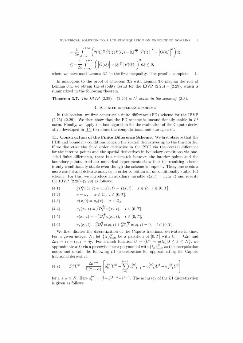
where we have used Lemma 3.1 in the first inequality. The proof is complete.

In analogous to the proof of Theorem 3.5 with Lemma 3.6 playing the role ofLemma 3.4, we obtain the stability result for the IBVP (2.25) – (2.29), which issummarized in the following theorem.

Theorem 3.7. The IBVP (2.25) – (2.29) is L2-stable in the sense of (3.3).

4. A finite difference scheme

In this section, we first construct a finite difference (FD) scheme for the IBVP(2.25)–(2.29). We then show that the FD scheme is unconditionally stable in L2

norm. Finally, we apply the fast algorithm for the evaluation of the Caputo deriv-ative developed in [15] to reduce the computational and storage cost.

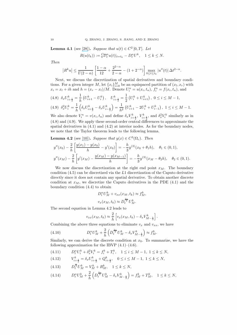
4.1. Construction of the Finite Difference Scheme. We first observe that thePDE and boundary conditions contain the spatial derivatives up to the third order.If we discretize the third order derivative in the PDE via the central differencefor the interior points and the spatial derivatives in boundary conditions via one-sided finite differences, there is a mismatch between the interior points and theboundary points. And our numerical experiments show that the resulting schemeis only conditionally stable even though the scheme is implicit. Thus, one needs amore careful and delicate analysis in order to obtain an unconditionally stable FDscheme. For this, we introduce an auxiliary variable v(x, t) = ux(x, t) and rewritethe IBVP (2.25)–(2.29) as follows:

C0D

αt u(x, t) + vxx(x, t) = f(x, t), x ∈ Ωc, t ∈ (0, T ],(4.1)

v = ux, x ∈ Ωc, t ∈ (0, T ],(4.2)

u(x, 0) = u0(x), x ∈ Ωc,(4.3)

vx(xr, t) =C0D

2α3

t u(xr, t), t ∈ (0, T ],(4.4)

v(xr , t) = −C0D

α

3

t u(xr, t), t ∈ (0, T ],(4.5)

vx(xl, t)−C0D

α

3

t v(xl, t) +C0D

2α3

t u(xl, t) = 0, t ∈ (0, T ].(4.6)

We first discuss the discretization of the Caputo fractional derivative in time.For a given integer N , let tk

Nk=0 be a partition of [0, T ] with tk = k∆t and

∆tk = tk − tk−1 = TN . For a mesh function U = Uk = u(tk)|0 ≤ k ≤ N, we

approximate u(t) via a piecewise linear polynomial with tkNk=0 as the interpolation

nodes and obtain the following L1 discretization for approximating the Caputofractional derivative:

Dαt U

k =∆t−α

Γ(2 − α)

[

a(α)0 Uk −

k−1∑

l=1

(a(α)k−l−1 − a

(α)k−l)U

l − a(α)k−1U

0

]

(4.7)

for 1 ≤ k ≤ N . Here a(α)l = (l+1)1−α− l1−α. The accuracy of the L1 discretization

is given as follows.

10 Q. ZHANG, J. ZHANG, S. JIANG, AND Z. ZHANG

Lemma 4.1 (see [28]). Suppose that u(t) ∈ C2 [0, T ]. Let

R(u(tk)) :=C0D

αt u(t)|t=tk −Dα

t Uk, 1 ≤ k ≤ N.

Then∣

∣Rku∣

∣ ≤1

Γ(2− α)

[

1− α

12+

22−α

2− α− (1 + 2−α)

]

max0≤t≤tk

|u′′(t)|∆t2−α.

Next, we discuss the discretization of spatial derivatives and boundary condi-tions. For a given integer M , let xi

Mi=0 be an equispaced partition of (xl, xr) with

xi = xl + ih and h = (xr − xl)/M . Denote Uni = u(xi, tn), f

ni = f(xi, tn), and

δxUki+ 1

2

=1

h

(

Uki+1 − Uk

i

)

, Uki+ 1

2

=1

2

(

Uki + Uk

i+1

)

, 0 ≤ i ≤ M − 1,(4.8)

δ2xUki =

1

h

(

δxUki+ 1

2

− δxUki− 1

2

)

=1

h2

(

Uki+1 − 2Uk

i + Uki−1

)

, 1 ≤ i ≤ M − 1.(4.9)

We also denote V ni = v(xi, tn) and define δxV

ki+ 1

2

, V ki+ 1

2

, and δ2xVki similarly as in

(4.8) and (4.9). We apply these second-order central differences to approximate thespatial derivatives in (4.1) and (4.2) at interior nodes. As for the boundary nodes,we note that the Taylor theorem leads to the following lemma.

Lemma 4.2 (see [10]). Suppose that y(x) ∈ C3(Ωc). Then

y′′(x0)−2

h

[

y(x1)− y(x0)

h− y′(x0)

]

= −h

3y(3)(x0 + θ1h), θ1 ∈ (0, 1),

y′′(xM )−2

h

[

y′(xM )−y(xM )− y(xM−1)

h

]

= −h

3y(3)(xM − θ2h), θ2 ∈ (0, 1).

We now discuss the discretization at the right end point xM . The boundarycondition (4.5) can be discretized via the L1 discretization of the Caputo derivativedirectly since it does not contain any spatial derivative. To obtain another discretecondition at xM , we discretize the Caputo derivatives in the PDE (4.1) and theboundary condition (4.4) to obtain

Dαt U

kM + vxx(xM , tk) ≈ fk

M ,

vx(xM , tk) ≈ D2α3

t UkM .

The second equation in Lemma 4.2 leads to

vxx(xM , tk) ≈2

h

[

vx(xM , tk)− δxVkM− 1

2

]

.

Combining the above three equations to eliminate vx and vxx, we have

(4.10) Dαt U

kM +

2

h

(

D2α3

t UkM − δxV

kM− 1

2

)

≈ fkM .

Similarly, we can derive the discrete condition at x0. To summarize, we have thefollowing approximation for the IBVP (4.1)–(4.6).

Dαt U

ki + δ2xV

ki = fk

i + T ki , 1 ≤ i ≤ M − 1, 1 ≤ k ≤ N,(4.11)

V ki+ 1

2

= δxUki+ 1

2

+Qki+ 1

2

, 0 ≤ i ≤ M − 1, 1 ≤ k ≤ N,(4.12)

Dα

3

t UkM = V k

M +RkM , 1 ≤ k ≤ N,(4.13)

Dαt U

kM +

2

h

(

D2α3

t UkM − δxV

kM− 1

2

)

= fkM + T k

M , 1 ≤ k ≤ N,(4.14)

NUMERICAL SOLUTION TO A LTF KDV EQUATION ON UNBOUNDED DOMAINS 11

Dαt U

k0 +

2

h

(

δxVk12

−Dα

3

t V k0 +D

2α3

t Uk0

)

= fk0 + T k

0 , 1 ≤ k ≤ N.(4.15)

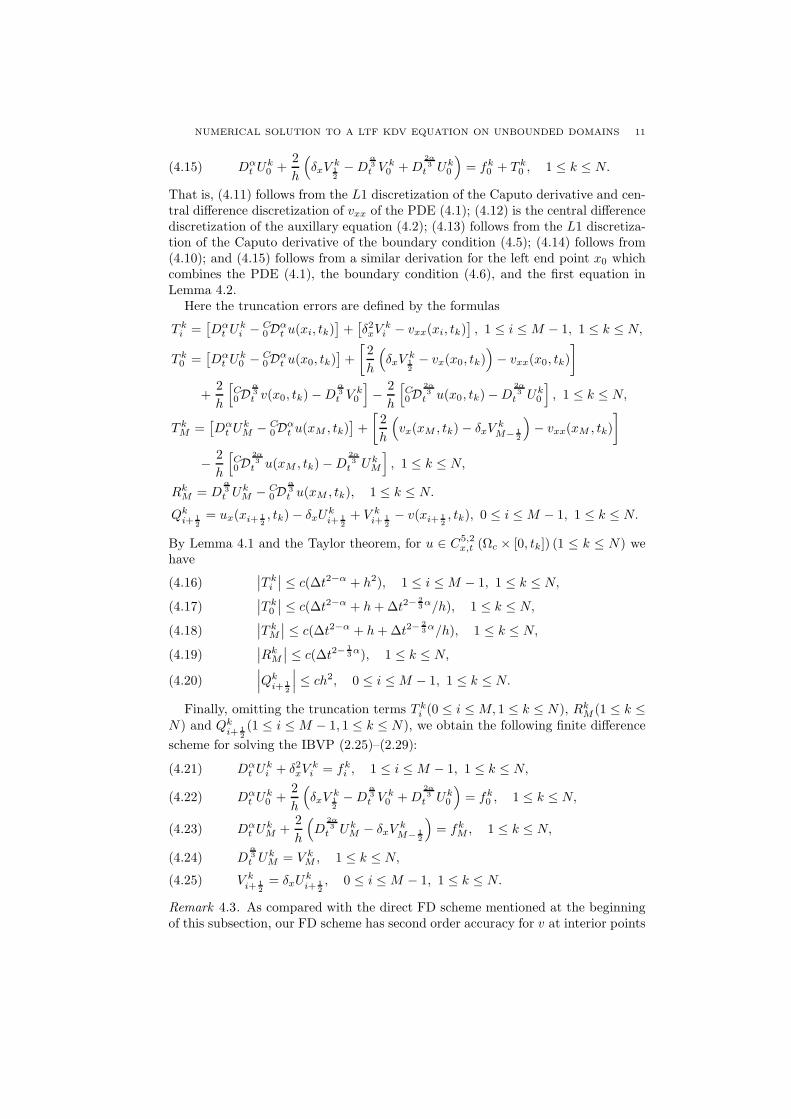
That is, (4.11) follows from the L1 discretization of the Caputo derivative and cen-tral difference discretization of vxx of the PDE (4.1); (4.12) is the central differencediscretization of the auxillary equation (4.2); (4.13) follows from the L1 discretiza-tion of the Caputo derivative of the boundary condition (4.5); (4.14) follows from(4.10); and (4.15) follows from a similar derivation for the left end point x0 whichcombines the PDE (4.1), the boundary condition (4.6), and the first equation inLemma 4.2.

Here the truncation errors are defined by the formulas

T ki =

[

Dαt U

ki − C

0Dαt u(xi, tk)

]

+[

δ2xVki − vxx(xi, tk)

]

, 1 ≤ i ≤ M − 1, 1 ≤ k ≤ N,

T k0 =

[

Dαt U

k0 − C

0Dαt u(x0, tk)

]

+

[

2

h

(

δxVk12

− vx(x0, tk))

− vxx(x0, tk)

]

+2

h

[

C0D

α

3

t v(x0, tk)−Dα

3

t V k0

]

−2

h

[

C0D

2α3

t u(x0, tk)−D2α3

t Uk0

]

, 1 ≤ k ≤ N,

T kM =

[

Dαt U

kM − C

0Dαt u(xM , tk)

]

+

[

2

h

(

vx(xM , tk)− δxVkM− 1

2

)

− vxx(xM , tk)

]

−2

h

[

C0D

2α3

t u(xM , tk)−D2α3

t UkM

]

, 1 ≤ k ≤ N,

RkM = D

α

3

t UkM − C

0Dα

3

t u(xM , tk), 1 ≤ k ≤ N.

Qki+ 1

2

= ux(xi+ 12, tk)− δxU

ki+ 1

2

+ V ki+ 1

2

− v(xi+ 12, tk), 0 ≤ i ≤ M − 1, 1 ≤ k ≤ N.

By Lemma 4.1 and the Taylor theorem, for u ∈ C5,2x,t (Ωc × [0, tk]) (1 ≤ k ≤ N) we

have∣

∣T ki

∣

∣ ≤ c(∆t2−α + h2), 1 ≤ i ≤ M − 1, 1 ≤ k ≤ N,(4.16)∣

∣T k0

∣

∣ ≤ c(∆t2−α + h+∆t2−23α/h), 1 ≤ k ≤ N,(4.17)

∣

∣T kM

∣

∣ ≤ c(∆t2−α + h+∆t2−23α/h), 1 ≤ k ≤ N,(4.18)

∣

∣RkM

∣

∣ ≤ c(∆t2−13α), 1 ≤ k ≤ N,(4.19)

∣

∣

∣Qk

i+ 12

∣

∣

∣≤ ch2, 0 ≤ i ≤ M − 1, 1 ≤ k ≤ N.(4.20)

Finally, omitting the truncation terms T ki (0 ≤ i ≤ M, 1 ≤ k ≤ N), Rk

M (1 ≤ k ≤N) and Qk

i+ 12

(1 ≤ i ≤ M − 1, 1 ≤ k ≤ N), we obtain the following finite difference

scheme for solving the IBVP (2.25)–(2.29):

Dαt U

ki + δ2xV

ki = fk

i , 1 ≤ i ≤ M − 1, 1 ≤ k ≤ N,(4.21)

Dαt U

k0 +

2

h

(

δxVk12

−Dα

3

t V k0 +D

2α3

t Uk0

)

= fk0 , 1 ≤ k ≤ N,(4.22)

Dαt U

kM +

2

h

(

D2α3

t UkM − δxV

kM− 1

2

)

= fkM , 1 ≤ k ≤ N,(4.23)

Dα

3

t UkM = V k

M , 1 ≤ k ≤ N,(4.24)

V ki+ 1

2

= δxUki+ 1

2

, 0 ≤ i ≤ M − 1, 1 ≤ k ≤ N.(4.25)

Remark 4.3. As compared with the direct FD scheme mentioned at the beginningof this subsection, our FD scheme has second order accuracy for v at interior points

12 Q. ZHANG, J. ZHANG, S. JIANG, AND Z. ZHANG

and first order accuracy at boundary points. Since v = ux, this implies third orderaccuracy for u at interior points and second order accuracy at boundary points.Thus, our FD scheme has higher order of accuracy and better stability property.

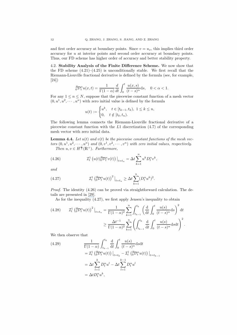
4.2. Stability Analysis of the Finite Difference Scheme. We now show thatthe FD scheme (4.21)–(4.25) is unconditionally stable. We first recall that theRiemann-Liouville fractional derivative is defined by the formula (see, for example,[24])

R0D

αt u(x, t) =

1

Γ(1− α)

d

dt

∫ t

0

u(x, s)

(t− s)αds, 0 < α < 1.

For any 1 ≤ n ≤ N , suppose that the piecewise constant function of a mesh vector(0, u1, u2, · · · , un) with zero initial value is defined by the formula

u(t) :=

uk, t ∈ [tk−1, tk), 1 ≤ k ≤ n,

0, t /∈ [t0, tn).

The following lemma connects the Riemann-Liouville fractional derivative of apiecewise constant function with the L1 discretization (4.7) of the correspondingmesh vector with zero initial data.

Lemma 4.4. Let u(t) and v(t) be the piecewise constant functions of the mesh vec-tors (0, u1, u2, · · · , un) and (0, v1, v2, · · · , vn) with zero initial values, respectively.

Then u, v ∈ Hα

3 (R+). Furthermore,

(4.26) I1t

(

u(t)R0Dαt v(t)

)∣

∣

t=tn= ∆t

n∑

k=1

ukDαt v

k,

and

(4.27) I1t

(

R0D

αt u(t)

)2 ∣∣

t=tn≥ ∆t

n∑

k=1

(Dαt u

k)2.

Proof. The identity (4.26) can be proved via straightforward calculation. The de-tails are presented in [29].

As for the inequality (4.27), we first apply Jensen’s inequality to obtain

I1t

(

R0D

αt u(t)

)2 ∣∣

t=tn=

1

Γ(1− α)2

n∑

k=1

∫ tk

tk−1

(

d

dt

∫ t

0

u(s)

(t− s)αds

)2

dt(4.28)

≥∆t−1

Γ(1− α)2

n∑

k=1

(

∫ tk

tk−1

d

dt

∫ t

0

u(s)

(t− s)αdsdt

)2

.

We then observe that

1

Γ(1− α)

∫ tk

tk−1

d

dt

∫ t

0

u(s)

(t− s)αdsdt(4.29)

= I1t

(

R0D

αt u(t)

)∣

∣

t=tk− I1

t

(

R0D

αt u(t)

)∣

∣

t=tk−1

= ∆t

k∑

l=1

Dαt u

l −∆t

k−1∑

l=1

Dαt u

l

= ∆tDαt u

k,

NUMERICAL SOLUTION TO A LTF KDV EQUATION ON UNBOUNDED DOMAINS 13

where the first equality follows from the fact that I1t is simply the integration

operator from 0 to t and the second equality follows from (4.26). Combining (4.28)and (4.29), we obtain (4.27).

Proceeding as in the proof of Lemma 3.6, we obtain the following lemma.

Lemma 4.5. For any T > 0, suppose f, g ∈ Hα

3 (0, T ). Then

I1t (2f

R0D

23α

t f − (R0Dα

3

t f)2)|t=T ≥ 0,(4.30)

I1t (2(

R0D

α

3

t g − R0D

23α

t f)f − g2)|t=T ≤ 0.(4.31)

The next lemma can be found in [10].

Lemma 4.6. For any mesh functions g = gk|0 ≤ k ≤ N defined on Ωt = tk|0 ≤k ≤ N, the following inequality holds:

∆tn∑

k=1

(Dαt g

k)gk ≥t−αn

2Γ(1− α)∆t

n∑

k=1

(gk)2 −t1−αn

2Γ(2− α)(g0)2, 1 ≤ n ≤ N.(4.32)

Let V = v|v = (v0, v1, · · · , vM ). For any U, V ∈ V, we define the inner productand norm as

(U, V ) = h

(

1

2U0V0 +

M−1∑

i=1

UiVi +1

2UMVM

)

, ‖U‖ =√

(U,U).

We now present the main theoretical result on the stability of the FD scheme.

Theorem 4.7. The finite difference scheme (4.21)–(4.25) is unconditionally stablewith respect to the initial data and the source term. That is,

∆tn∑

k=1

∥

∥Uk∥

∥

2≤

2tn1− α

∥

∥U0∥

∥

2+ 4t2αn Γ(1− α)2∆t

n∑

k=1

∥

∥fk∥

∥

2, 1 ≤ n ≤ N.(4.33)

Proof. We multiply both sides of (4.21) by hUki , and then sum up for i from 1

to M − 1; we then multiply both sides of (4.22) and (4.23) by h2U

k0 and h

2UkM ,

respectively; finally we add up these equations to obtain

(

Dαt U

k, Uk)

+

M−1∑

i=1

hδ2xVki · Uk

i + δxVk12

· Uk0 − δxV

kM− 1

2

· UkM(4.34)

−Dα

3

t V k0 · Uk

0 +D2α3

t Uk0 · Uk

0 +D2α3

t UkM · Uk

M = (fk, Uk).

We then use (4.25) to simplify the second term to the fourth term of the left sidein (4.34),

M−1∑

i=1

hδ2xVki · Uk

i + δxV 12· Uk

0 − δxVM− 12· Uk

M(4.35)

=

M−1∑

i=1

(δxVki+ 1

2

− δxVki− 1

2

) · Uki + δxV 1

2Uk0 − δxVM− 1

2UkM

=

M∑

i=1

δxVki− 1

2

(Uki−1 − Uk

i ) =

M∑

i=1

(

V ki−1 − V k

i

)

δxUki− 1

2

14 Q. ZHANG, J. ZHANG, S. JIANG, AND Z. ZHANG

=

M∑

i=1

(

V ki−1

)2−(

V ki

)2

2=

1

2(V k

0 )2 −1

2(V k

M )2

Substituting (4.35) and (4.24) into (4.34), we obtain

(

Dαt U

k, Uk)

+1

2(V k

0 )2 −Dα

3

t V k0 · Uk

0 +D2α3

t Uk0 · Uk

0(4.36)

−1

2

(

Dα

3

t UkM

)2

+D2α3

t UkM · Uk

M = (fk, Uk).

Multiplying ∆t on both sides of the (4.36), summing up for k from 1 to n, andapplying the identity (4.26), we obtain

n∑

k=1

∆t(

Dαt U

k, Uk)

+ I1t

(

1

2(V0)

2 − (R0Dα

3

t V0)U0 + (R0D2α3

t U0)U0

)

∣

∣

∣

t=tn(4.37)

+ I1t

(

(R0D2α3

t UM )UM −1

2

(

R0D

α

3

t UM

)2)

∣

∣

∣

t=tn=

n∑

k=1

∆t(fk, Uk).

Here U0, V0, UM are piecewise constant functions of the mesh vectors (U00 , U

10 , · · · , U

n0 ),

(V 00 , V

10 , · · · , V

n0 ), and (U0

M , U1M , · · · , Un

M ), respectively. And we have used the factthat U0

M = U00 = V 0

0 = 0 by the assumption that the initial data are compactlysupported.

By the inequality (4.31), the second term on the left side of (4.37) is nonnegative;by the inequality (4.30), the third term on the left side of (4.37) is nonnegative.Thus,

n∑

k=1

∆t(

Dαt U

k, Uk)

≤

n∑

k=1

∆t(fk, Uk).(4.38)

Applying the inequality (4.32) to estimate the left side of (4.38), we have

t−αn

2Γ(1− α)∆t

n∑

k=1

∥

∥Uk∥

∥

2≤

t1−αn

2Γ(2− α)

∥

∥U0∥

∥

2+

n∑

k=1

∆t(fk, Uk).(4.39)

Now the Cauchy-Schwarz inequality yields

(fk, Uk) ≤∥

∥fk∥

∥ ·∥

∥Uk∥

∥(4.40)

≤ tαnΓ(1− α)∥

∥fk∥

∥

2+

t−αn

4Γ(1− α)

∥

∥Uk∥

∥

2.

Finally, combining (4.39) with (4.40) and simplifying the resulting expression, weobtain (4.33).

4.3. Acceleration of the Finite Difference Scheme. The direct implementa-tion of the FD scheme (4.21)–(4.25) is very expensive in both the computationaland storage cost. This is because the Caputo derivative is a nonlocal operator andits L1 discretization (or any consistent discretization) contains a summation thatinvolves all values of the solution up to the current time. Hence, one needs to storeall previous solution values and the total cost of evaluating the L1 discretization ateach spatial point is O(N2) with N the total number of time steps.

We apply the fast algorithm for the evaluation of the Caputo fractional derivativein [15] to reduce the computational and storage cost. In order to make the papermore or less self-contained, we present a short summary of the algorithm in [15]

NUMERICAL SOLUTION TO A LTF KDV EQUATION ON UNBOUNDED DOMAINS 15

here. We first split the fractional Caputo derivative into a sum of local part andhistory part

C0D

αt u(t)|t=tk =

1

Γ(1− α)

∫ tk

tk−1

u′(s)ds

(tk − s)α+

1

Γ(1− α)

∫ tk−1

0

u′(s)ds

(tk − s)α

:= Cl(tk) + Ch(tk).(4.41)

For the local part Cl(tk), we apply the L1 approximation in the form

Cl(tk) ≈u(tk)− u(tk−1)

∆tkΓ(1− α)

∫ tk

tk−1

1

(tk − s)αds =

u(tk)− u(tk−1)

∆tαkΓ(2− α).(4.42)

For the history part Ch(tk), we first perform integration by parts to obtain

Ch(tk) =1

Γ(1− α)

[

u(tk−1)

∆tαk−

u(t0)

tαk− α

∫ tk−1

0

u(s)ds

(tk − s)1+α

]

.(4.43)

Obviously, the most work is on the evaluation of the convolution integral with thekernel 1

t1+α on the right side of (4.43). It has been shown in [15] that there exists

an efficient sum-of-exponentials approximation for 1t1+α for any given time interval

[∆tk, T ] with a prescribe absolute error ε. To be more precise, there exist positivereal numbers si and wi (i = 1, · · · , Nexp) such that

(4.44)

∣

∣

∣

∣

∣

∣

1

t1+α−

Nexp∑

i=1

ωie−sit

∣

∣

∣

∣

∣

∣

≤ ε, t ∈ [∆t, T ];

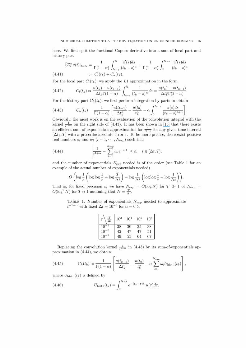
and the number of exponentials Nexp needed is of the order (see Table 1 for anexample of the actual number of exponentials needed)

O

(

log1

ε

(

log log1

ε+ log

T

∆t

)

+ log1

∆t

(

log log1

ε+ log

1

∆t

))

.

That is, for fixed precision ε, we have Nexp = O(logN) for T ≫ 1 or Nexp =

O(log2 N) for T ≈ 1 assuming that N = T∆t .

Table 1. Number of exponentials Nexp needed to approximatet−1−α with fixed ∆t = 10−3 for α = 0.5.

ε

∖

T∆t 103 104 105 106

10−3 28 30 35 3810−6 42 47 47 5110−9 49 55 64 67

Replacing the convolution kernel 1t1+α in (4.43) by its sum-of-exponentials ap-

proximation in (4.44), we obtain

Ch(tk) ≈1

Γ(1− α)

u(tk−1)

∆tαk−

u(t0)

tαk− α

Nexp∑

i=1

ωiUhist,i(tk)

,(4.45)

where Uhist,i(tk) is defined by

(4.46) Uhist,i(tk) =

∫ tk−1

0

e−(tk−τ)siu(τ)dτ.

16 Q. ZHANG, J. ZHANG, S. JIANG, AND Z. ZHANG

The reduction of the computational and storage cost relies on the fact that Uhist,i(tk)satisfies a simple recurrence relation

(4.47) Uhist,i(tk) = e−si∆tkUhist,i(tk−1) +

∫ tk−1

tk−2

e−si(tk−τ)u(τ)dτ

with Uhist,i(t0) = 0 for i = 1, · · · , Nexp. The integral on the right hand side of(4.47) can be calculated by a linear approximation of u followed with a productintegration. That is,

∫ tk−1

tk−2

e−si(tk−τ)u(τ)dτ ≈e−si∆tk

s2i∆tk−1

[

(e−si∆tk−1 − 1 + si∆tk−1)Uk−1(4.48)

+(1− e−si∆tk−1 − e−si∆tk−1si∆tk−1)Uk−2]

.

Thus, one only needs O(1) cost to compute Uhist,i(tk) at each step as Uhist,i(tk−1)is already computed and stored. As there are Nexp history modes altogether, thecost of evaluating the Caputo derivative at each time step is O(Nexp). That is, a

reduction from O(N) to O(logN) or O(log2 N).To summarize, the fast evaluation of the Caputo derivative can be implemented

by the formula

C0D

αt U

k ≈Uk − Uk−1

∆tαkΓ(2− α)+

1

Γ(1− α)

Uk−1

∆tαk−

U0

tαk− α

Nexp∑

i=1

ωiUhist,i(tk)

(4.49)

=: FDαt U

k, for k > 0,

where Uhist,i(tk) is evaluated via (4.47) and (4.48). Finally, replacing the L1 dis-cretization Dα

t Uk by its fast version FDα

t Uk in the FD scheme (4.21)–(4.25), we

obtain an accelerated FD scheme as follows.

FDαt U

ki + δ2xV

ki = fk

i , 1 ≤ i ≤ M − 1, 1 ≤ k ≤ N,(4.50)

FDαt U

k0 +

2

h

(

δxVk12

− FDα

3

t V k0 + FD

2α3

t Uk0

)

= fk0 , 1 ≤ k ≤ N,(4.51)

FDαt U

kM +

2

h

(

FD2α3

t UkM − δxV

kM− 1

2

)

= fkM , 1 ≤ k ≤ N,(4.52)

FDα

3

t UkM = V k

M , 1 ≤ k ≤ N,(4.53)

V ki+ 1

2

= δxUki+ 1

2

, 0 ≤ i ≤ M − 1, 1 ≤ k ≤ N.(4.54)

Remark 4.8. The fast algorithm relies on the fact that the convolution with theexponential kernel can be evaluated in linear time since it is equivalent to solvingan ordinary differential equation (ODE). Thus it can be applied to adaptive timemarching scheme as well. The only penalty here is that the number of exponentialswill increase slightly due to the decrease of the smallest time step.

Remark 4.9. Another fast algorithm for the evaluation of the fractional derivativehas been proposed in [4], where the compression is carried out in the Laplacedomain, and the convolution with an exponential kernel is computed by solving theequivalent ODE with some one-step A-stable scheme.

Remark 4.10. Both the L1 discretization Dαt U

k and the fast algorithm FDαt U

k

approximate u(t) by a piecewise polynomial and then apply the product integration.Therefore, the difference is very minor and can in fact be made arbitrarily small if

NUMERICAL SOLUTION TO A LTF KDV EQUATION ON UNBOUNDED DOMAINS 17

the prescribed precision ε is set to a small number, say, close to machine precision.In our numerical experiments, we have not observed any significant differencesbetween the FD scheme (4.21)–(4.25) and its fast version (4.50)–(4.54) in bothaccuracy and stability.

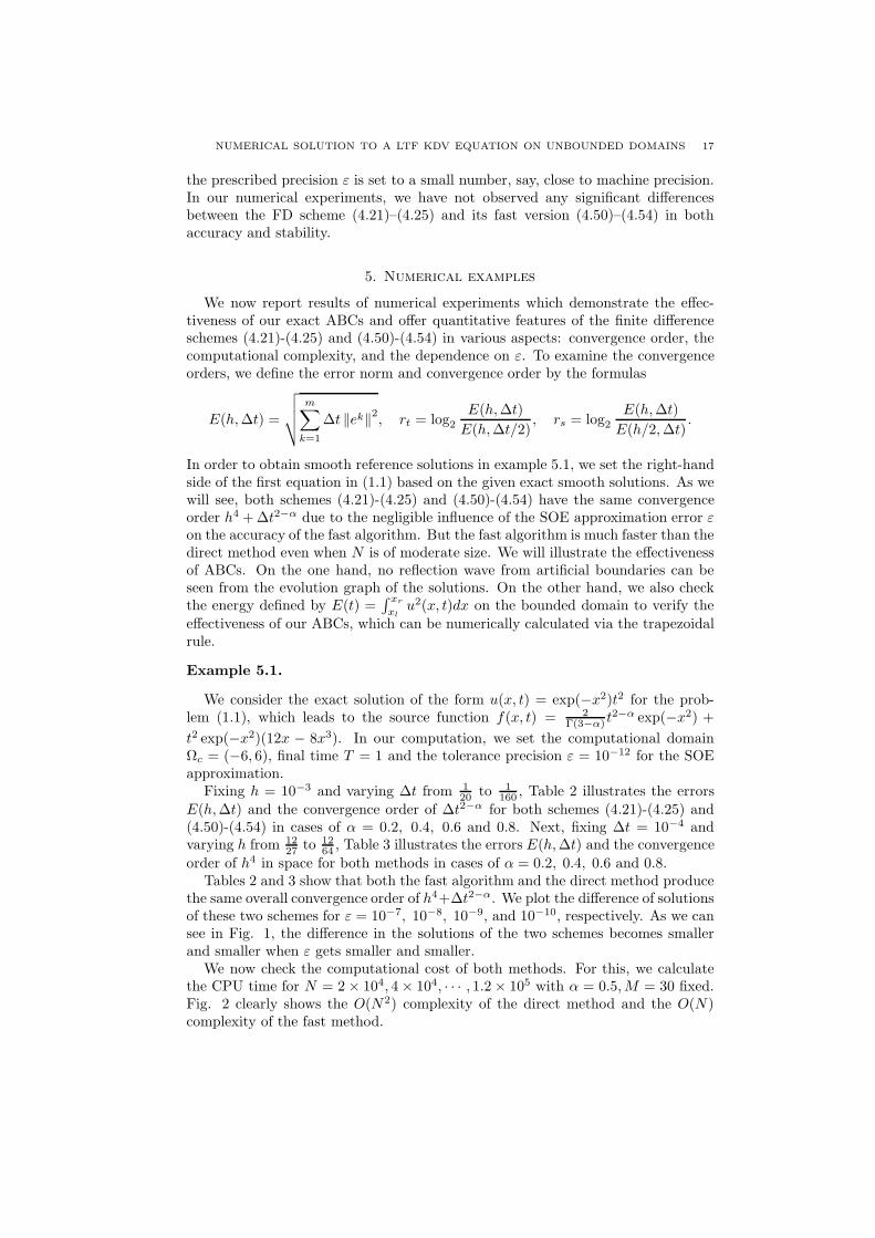
5. Numerical examples

We now report results of numerical experiments which demonstrate the effec-tiveness of our exact ABCs and offer quantitative features of the finite differenceschemes (4.21)-(4.25) and (4.50)-(4.54) in various aspects: convergence order, thecomputational complexity, and the dependence on ε. To examine the convergenceorders, we define the error norm and convergence order by the formulas

E(h,∆t) =

√

√

√

√

m∑

k=1

∆t ‖ek‖2, rt = log2

E(h,∆t)

E(h,∆t/2), rs = log2

E(h,∆t)

E(h/2,∆t).

In order to obtain smooth reference solutions in example 5.1, we set the right-handside of the first equation in (1.1) based on the given exact smooth solutions. As wewill see, both schemes (4.21)-(4.25) and (4.50)-(4.54) have the same convergenceorder h4 +∆t2−α due to the negligible influence of the SOE approximation error εon the accuracy of the fast algorithm. But the fast algorithm is much faster than thedirect method even when N is of moderate size. We will illustrate the effectivenessof ABCs. On the one hand, no reflection wave from artificial boundaries can beseen from the evolution graph of the solutions. On the other hand, we also checkthe energy defined by E(t) =

∫ xr

xl

u2(x, t)dx on the bounded domain to verify the

effectiveness of our ABCs, which can be numerically calculated via the trapezoidalrule.

Example 5.1.

We consider the exact solution of the form u(x, t) = exp(−x2)t2 for the prob-lem (1.1), which leads to the source function f(x, t) = 2

Γ(3−α) t2−α exp(−x2) +

t2 exp(−x2)(12x − 8x3). In our computation, we set the computational domainΩc = (−6, 6), final time T = 1 and the tolerance precision ε = 10−12 for the SOEapproximation.

Fixing h = 10−3 and varying ∆t from 120 to 1

160 , Table 2 illustrates the errors

E(h,∆t) and the convergence order of ∆t2−α for both schemes (4.21)-(4.25) and(4.50)-(4.54) in cases of α = 0.2, 0.4, 0.6 and 0.8. Next, fixing ∆t = 10−4 andvarying h from 12

27 to 1264 , Table 3 illustrates the errors E(h,∆t) and the convergence

order of h4 in space for both methods in cases of α = 0.2, 0.4, 0.6 and 0.8.Tables 2 and 3 show that both the fast algorithm and the direct method produce

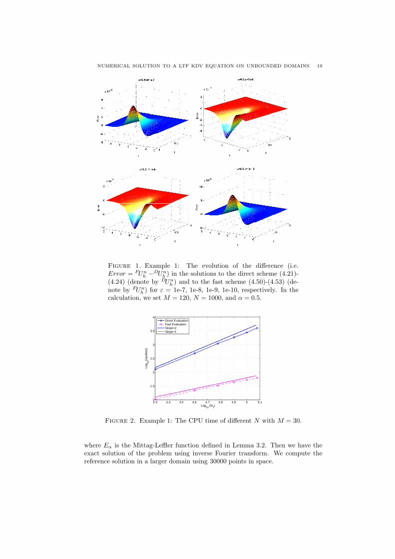
the same overall convergence order of h4+∆t2−α. We plot the difference of solutionsof these two schemes for ε = 10−7, 10−8, 10−9, and 10−10, respectively. As we cansee in Fig. 1, the difference in the solutions of the two schemes becomes smallerand smaller when ε gets smaller and smaller.

We now check the computational cost of both methods. For this, we calculatethe CPU time for N = 2 × 104, 4× 104, · · · , 1.2× 105 with α = 0.5,M = 30 fixed.Fig. 2 clearly shows the O(N2) complexity of the direct method and the O(N)complexity of the fast method.

18 Q. ZHANG, J. ZHANG, S. JIANG, AND Z. ZHANG

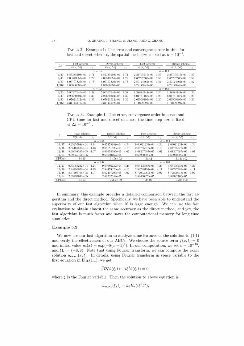
Table 2. Example 1: The error and convergence order in time forfast and direct schemes, the spatial mesh size is fixed at h = 10−3.

∆tFast scheme Direct scheme Fast scheme Direct scheme

E(h,∆t) rt E(h,∆t) rt E(h,∆t) rt E(h,∆t) rtα = 0.2 α = 0.4

1/20 6.55385108e-04 1.71 6.55385108e-04 1.71 2.24705517e-03 1.55 2.24705517e-03 1.551/40 2.00843055e-04 1.72 2.00843055e-04 1.72 7.65737566e-04 1.56 7.65737566e-04 1.561/80 6.09797829e-05 1.73 6.09797829e-05 1.73 2.59174561e-04 1.57 2.59174561e-04 1.571/160 1.83606636e-05 1.83606636e-05 8.72173249e-05 8.72173249e-05

α = 0.6 α = 0.81/20 5.90307640e-03 1.38 5.90307640e-03 1.38 1.38884744e-02 1.20 1.38884744e-02 1.201/40 2.26680324e-03 1.39 2.26680324e-03 1.39 6.04731488e-03 1.20 6.04731488e-03 1.201/80 8.67621912e-04 1.39 8.67621912e-04 1.39 2.63569499e-03 1.20 2.63569499e-03 1.201/160 3.31144112e-04 3.31144112e-04 1.14869621e-03 1.14869621e-03

Table 3. Example 1: The error, convergence order in space andCPU time for fast and direct schemes, the time step size is fixedat ∆t = 10−4 .

hFast scheme Direct scheme Fast scheme Direct scheme

E(h,∆t) rs E(h,∆t) rs E(h,∆t) rs E(h,∆t) rsα = 0.2 α = 0.4

12/27 9.65355988e-04 4.24 9.65355988e-04 4.24 9.64031334e-04 4.24 9.64031334e-04 4.2412/36 2.85181520e-04 4.13 2.85181520e-04 4.13 2.84755576e-04 4.13 2.84755576e-04 4.1312/48 8.69658395e-05 4.07 8.69658395e-05 4.07 8.68307687e-05 4.07 8.68307687e-05 4.0712/64 2.69650162e-05 2.69650162e-05 2.69230020e-05 2.69230020e-05CPU(s) 34.50 3.19e+02 34.42 3.34e+02

α = 0.6 α = 0.812/27 9.63086232e-04 4.24 9.63086232e-04 4.24 9.63498568e-04 4.24 9.63498738e-04 4.2412/36 2.84459020e-04 4.13 2.84459020e-04 4.13 2.84788157e-04 4.11 2.84787989e-04 4.1112/48 8.67497706e-05 4.07 8.67497706e-05 4.07 8.72903060e-05 3.92 8.72890018e-05 3.9212/64 2.69232642e-05 2.69232642e-05 2.82430370e-05 2.82382760e-05CPU(s) 34.53 3.30e+02 35.06 3.30e+02

In summary, this example provides a detailed comparison between the fast al-gorithm and the direct method. Specifically, we have been able to understand thesuperiority of our fast algorithm when N is large enough. We can use the fastevaluation to obtain almost the same accuracy as the direct method, and yet, thefast algorithm is much faster and saves the computational memory for long timesimulation.

Example 5.2.

We now use our fast algorithm to analyze some features of the solution to (1.1)and verify the effectiveness of our ABCs. We choose the source term f(x, t) = 0and initial value u0(x) = exp(−8(x − 5)2). In our computation, we set ε = 10−10,and Ωc = (−8, 8). Note that using Fourier transform, we can compute the exactsolution uexact(x, t). In details, using Fourier transform in space variable to thefirst equation in E.q.(1.1), we get

C0D

αt u(ξ, t)− iξ3u(ξ, t) = 0,

where ξ is the Fourier variable. Then the solution to above equation is

uexact(ξ, t) = u0Eα(iξ3tα),

NUMERICAL SOLUTION TO A LTF KDV EQUATION ON UNBOUNDED DOMAINS 19

Figure 1. Example 1: The evolution of the difference (i.e.Error = FUn

h −DUnh ) in the solutions to the direct scheme (4.21)-

(4.24) (denote by DUnh ) and to the fast scheme (4.50)-(4.53) (de-

note by FUnh ) for ε = 1e-7, 1e-8, 1e-9, 1e-10, respectively. In the

calculation, we set M = 120, N = 1000, and α = 0.5.

4.3 4.4 4.5 4.6 4.7 4.8 4.9 5 5.11

1.5

2

2.5

3

3.5

4

Log10

(NT)

Log 10

(cpu

time)

Direct EvaluationFast EvaluationSlope=2Slope=1

Figure 2. Example 1: The CPU time of different N with M = 30.

where Eα is the Mittag-Leffler function defined in Lemma 3.2. Then we have theexact solution of the problem using inverse Fourier transform. We compute thereference solution in a larger domain using 30000 points in space.

20 Q. ZHANG, J. ZHANG, S. JIANG, AND Z. ZHANG

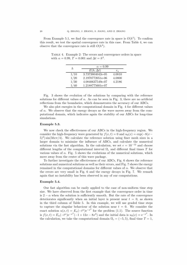
From Example 5.1, we find the convergence rate in space is O(h4). To confirmthis result, we test the spatial convergence rate in this case. From Table 4, we canobserve that the convergence rate is still O(h4).

Table 4. Example 2: The errors and convergence orders in spacewith α = 0.99, T = 0.001 and ∆t = h4.

hα = 0.99

E(h,∆t) rs1/10 3.7373804042e-05 4.08101/20 2.1970772051e-06 4.08001/30 4.0840637549e-07 4.21861/40 1.2188775601e-07

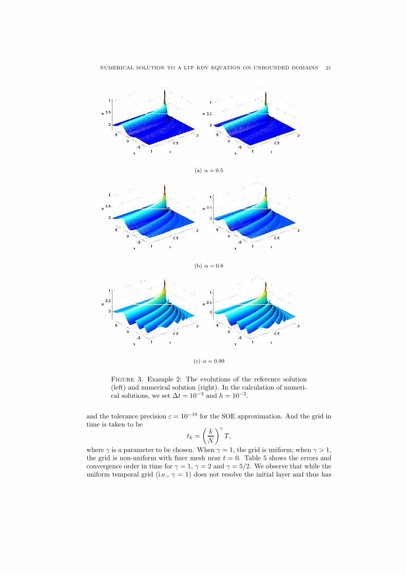
Fig. 3 shows the evolution of the solutions by comparing with the referencesolutions for different values of α. As can be seen in Fig. 3, there are no artificialreflections from the boundaries, which demonstrates the accuracy of our ABCs.

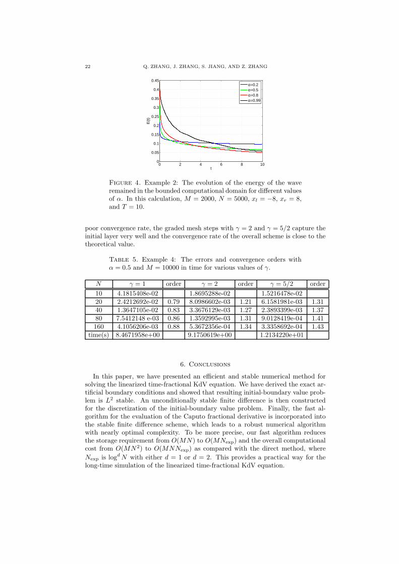
We also plot energies in the computational domain in Fig. 4 for different valuesof α. We observe that the energy decays as the wave moves away from the com-putational domain, which indicates again the stability of our ABCs for long-timesimulations.

Example 5.3.

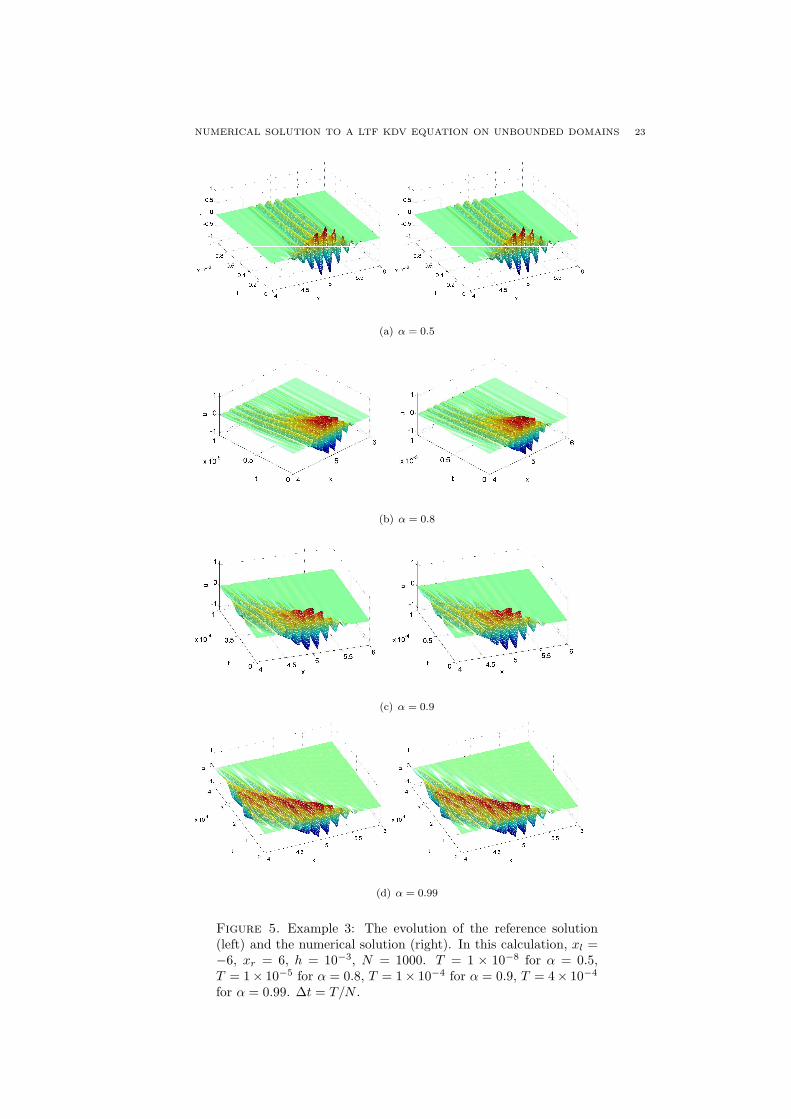
We now check the effectiveness of our ABCs in the high-frequency region. Weconsider the high-frequency wave generated by f(x, t) = 0 and u0(x) = exp(−8(x−5)2) sin(50xπ/4). We calculate the reference solution using finer mesh sizes in alarger domain to minimize the influence of ABCs, and calculate the numericalsolutions via the fast algorithm. In the calculation, we set ǫ = 10−12 and choosedifferent lengths of the computational interval Ωc and different final times T forvarious values of α. Fig. 5 shows the evolutions of the numerical solutions, whichmove away from the center of this wave package.

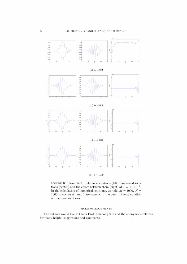
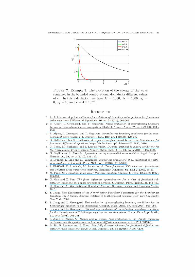
To further investigate the effectiveness of our ABCs, Fig. 6 shows the referencesolutions and numerical solutions as well as their errors, and Fig. 7 shows the energyremained in the computational domains for different values of α. We observe thatthe errors are very small in Fig. 6 and the energy decays in Fig. 7. We remarkagain that no instability has been observed in any of our computations.

Example 5.4.

Our fast algorithm can be easily applied to the case of non-uniform time stepsize. We have observed from the first example that the convergence order in timeis 2 − α when the solution is sufficiently smooth. But the rate of the convergencedeteriorates significantly when an initial layer is present near t = 0, as shownin the third column of Table 5. In this example, we will use graded time stepsto capture the singular behaviour of the solution near t = 0. We consider the

exact solution u(x, t) = Eα(−tα)e−x2

for the problem (1.1). The source function

is f(x, t) = Eα(−tα)e−x2

(−1 + 12x− 8x3) and the initial data is u0(x) = e−x2

. Inthe calculation, we take the computational domain Ωc = (−5, 5), final time T = 1,

NUMERICAL SOLUTION TO A LTF KDV EQUATION ON UNBOUNDED DOMAINS 21

(a) α = 0.5

(b) α = 0.8

(c) α = 0.99

Figure 3. Example 2: The evolutions of the reference solution(left) and numerical solution (right). In the calculation of numeri-cal solutions, we set ∆t = 10−3 and h = 10−3.

and the tolerance precision ε = 10−10 for the SOE approximation. And the grid intime is taken to be

tk =

(

k

N

)γ

T,

where γ is a parameter to be chosen. When γ = 1, the grid is uniform; when γ > 1,the grid is non-uniform with finer mesh near t = 0. Table 5 shows the errors andconvergence order in time for γ = 1, γ = 2 and γ = 5/2. We observe that while theuniform temporal grid (i.e., γ = 1) does not resolve the initial layer and thus has

22 Q. ZHANG, J. ZHANG, S. JIANG, AND Z. ZHANG

0 2 4 6 8 100

0.05

0.1

0.15

0.2

0.25

0.3

0.35

0.4

0.45

t

E(t

)

α=0.2α=0.5α=0.8α=0.99

Figure 4. Example 2: The evolution of the energy of the waveremained in the bounded computational domain for different valuesof α. In this calculation, M = 2000, N = 5000, xl = −8, xr = 8,and T = 10.

poor convergence rate, the graded mesh steps with γ = 2 and γ = 5/2 capture theinitial layer very well and the convergence rate of the overall scheme is close to thetheoretical value.

Table 5. Example 4: The errors and convergence orders withα = 0.5 and M = 10000 in time for various values of γ.

N γ = 1 order γ = 2 order γ = 5/2 order

10 4.1815408e-02 1.8695288e-02 1.5216478e-0220 2.4212692e-02 0.79 8.0986602e-03 1.21 6.1581981e-03 1.3140 1.3647105e-02 0.83 3.3676129e-03 1.27 2.3893399e-03 1.3780 7.5412148 e-03 0.86 1.3592995e-03 1.31 9.0128419e-04 1.41160 4.1056206e-03 0.88 5.3672356e-04 1.34 3.3358692e-04 1.43

time(s) 8.4671958e+00 9.1750619e+00 1.2134220e+01

6. Conclusions

In this paper, we have presented an efficient and stable numerical method forsolving the linearized time-fractional KdV equation. We have derived the exact ar-tificial boundary conditions and showed that resulting initial-boundary value prob-lem is L2 stable. An unconditionally stable finite difference is then constructedfor the discretization of the initial-boundary value problem. Finally, the fast al-gorithm for the evaluation of the Caputo fractional derivative is incorporated intothe stable finite difference scheme, which leads to a robust numerical algorithmwith nearly optimal complexity. To be more precise, our fast algorithm reducesthe storage requirement from O(MN) to O(MNexp) and the overall computationalcost from O(MN2) to O(MNNexp) as compared with the direct method, where

Nexp is logdN with either d = 1 or d = 2. This provides a practical way for thelong-time simulation of the linearized time-fractional KdV equation.

NUMERICAL SOLUTION TO A LTF KDV EQUATION ON UNBOUNDED DOMAINS 23

(a) α = 0.5

(b) α = 0.8

(c) α = 0.9

(d) α = 0.99

Figure 5. Example 3: The evolution of the reference solution(left) and the numerical solution (right). In this calculation, xl =−6, xr = 6, h = 10−3, N = 1000. T = 1 × 10−8 for α = 0.5,T = 1× 10−5 for α = 0.8, T = 1× 10−4 for α = 0.9, T = 4× 10−4

for α = 0.99. ∆t = T/N .

24 Q. ZHANG, J. ZHANG, S. JIANG, AND Z. ZHANG

4 4.5 5 5.5 6

−0.01

−0.008

−0.006

−0.004

−0.002

0

0.002

0.004

0.006

0.008

0.01

x

u

4 4.5 5 5.5 6

−0.01

−0.008

−0.006

−0.004

−0.002

0

0.002

0.004

0.006

0.008

0.01

x

u

4 4.5 5 5.5 6

−5

−4

−3

−2

−1

0

x 10−4

x

erro

r

(a) α = 0.2

4 4.5 5 5.5 6−1

−0.8

−0.6

−0.4

−0.2

0

0.2

0.4

0.6

0.8

1

x

u

4 4.5 5 5.5 6−1

−0.8

−0.6

−0.4

−0.2

0

0.2

0.4

0.6

0.8

1

x

u

4 4.5 5 5.5 6−2

−1

0

1

2

3

x 10−4

x

erro

r

(b) α = 0.5

4 4.5 5 5.5 6

−1

−0.8

−0.6

−0.4

−0.2

0

0.2

0.4

0.6

0.8

1

x

u

4 4.5 5 5.5 6

−1

−0.8

−0.6

−0.4

−0.2

0

0.2

0.4

0.6

0.8

1

x

u

4 4.5 5 5.5 6

−2

−1.5

−1

−0.5

0

0.5

1

1.5

2

2.5

3

x 10−4

x

erro

r

(c) α = 0.8

4 4.5 5 5.5 6

−1

−0.8

−0.6

−0.4

−0.2

0

0.2

0.4

0.6

0.8

1

x

u

4 4.5 5 5.5 6

−1

−0.8

−0.6

−0.4

−0.2

0

0.2

0.4

0.6

0.8

1

x

u

4 4.5 5 5.5 6

−1.5

−1

−0.5

0

0.5

1

1.5

2

x 10−4

x

erro

r

(d) α = 0.99

Figure 6. Example 3: Reference solutions (left), numerical solu-tions (center) and the errors between them (right) at T = 1×10−6.In the calculation of numerical solutions, we take M = 1000, N =1000 to ensure ∆t and h are same with the ones in the calculationof reference solutions.

Acknowledgements

The authors would like to thank Prof. Zhizhong Sun and the anonymous refereesfor many helpful suggestions and comments.

NUMERICAL SOLUTION TO A LTF KDV EQUATION ON UNBOUNDED DOMAINS 25

0 1 2 3 4

x 10−4

0

0.05

0.1

0.15

0.2

0.25

t

E(t

)

α=0.5α=0.8α=0.9α=0.99

Figure 7. Example 3: The evolution of the energy of the waveremained in the bounded computational domain for different valuesof α. In this calculation, we take M = 1000, N = 1000, xl =0, xr = 10 and T = 4× 10−4.

References

1. A. Alikhanov. A priori estimates for solutions of boundary value problem for fractional-

order equations. Differential Equations, 46, no. 5 (2011), 660-666.2. B. Alpert, L. Greengard, and T. Hagstrom. Rapid evaluation of nonreflecting boundary

kernels for time-domain wave propagation. SIAM J. Numer. Anal., 37, no. 4 (2000), 1138-1164.

3. B. Alpert, L. Greengard, and T. Hagstrom. Nonreflecting boundary conditions for the time-

dependent wave equation. J. Comput. Phys., 180, no. 1 (2002), 270-296.4. D. Baffet and Jan S. Hesthaven, A Laplace transform based kernel reduction scheme for

fractional differential equations, https://infoscience.epfl.ch/record/212955, 2016.5. C. Besse, M. Ehrhardt, and I. Lacroix-Violet. Discrete artificial boundary conditions for

the Korteweg-de Vries equation. Numer. Meth. Part. D. E., 32, no. 5(2016), 1455-1484.6. G. Beylkin and L. Monzon. Approximation by exponential sums revisited. Appl. Comput.

Harmon. A., 28, no. 2 (2010), 131-149.7. H. Brunner, L. Ling and M. Yamamoto. Numerical simulations of 2D fractional sub diffu-

sion problems. J. Comput. Phys., 229, no.18 (2010), 6613-6622.8. S. El-Wakil, E. Abulwafa, M. Zahran et al. Time-fractional KdV equation: formulation

and solution using variational methods. Nonlinear Dynamics, 65, no.1-2(2009), 55-63.9. M. Fung. KdV equation as an Euler-Poincare equation. Chinese J. Phys., 35,no.6S(1997),

789-796.10. G. Gao and Z. Sun, The finite difference approximation for a class of fractional sub-

diffusion equations on a space unbounded domain, J. Comput. Phys., 236(2013), 443–460.11. H. Han and X. Wu. Artificial Boundary Method. Springer Science and Business Media,

2013.12. S. Jiang. Fast Evaluation of the Nonreflecting Boundary Conditions for the Schrodinger

Equation. Ph.D. thesis, Courant Institute of Mathematical Sciences, New York University,New York, 2001.

13. S. Jiang and L. Greengard. Fast evaluation of nonreflecting boundary conditions for the

Schrodinger equation in one dimension. Comput. Math. Appl. 47, no.6(2004), 955–966.14. S. Jiang and L. Greengard. Efficient representation of nonreflecting boundary conditions

for the time-dependent Schrodinger equation in two dimensions. Comm. Pure Appl. Math.,61, no.2 (2008), 261-288.

15. S. Jiang, J. Zhang, Q. Zhang, and Z. Zhang. Fast evaluation of the Caputo fractional

derivative and its applications to fractional diffusion equations. arXiv:1511.03453v1.16. B. Jin, R. Lazarov and Z. Zhou. Two fully discrete schemes for fractional diffusion and

diffusion wave equations. SIAM J. Sci. Comput., 38, no.1(2016), A146-A170.

26 Q. ZHANG, J. ZHANG, S. JIANG, AND Z. ZHANG

17. L. Jose, O. Eugene, and S. Martin. Error analysis of a finite difference method for a time-

fractional advection-diffusion equation. To appear, 2015.18. A. Kilbas, H. Srivastava, and J. Trujillo. Theory and Applications of Fractional Differential

Equations, Elesvier Science and Technology, Boston, 2006.19. D. Korteweg and G. de Vries. On the change of form of long waves advancing in a rect-

angular canal, and on a new type of long stationary waves. Philosophical Magazine, 39,no.240 (1895), 422-443.

20. T. Langlands and B. Henry. Fractional chemotaxis diffusion equations. Phys. Rev. E, 81,no.5(2010), 051102.

21. J. Li. A fast time stepping method for evaluating fractional integrals. SIAM J. Sci. Comput.,31, no. 6 (2009), 4696-4714.

22. R. Metzler and J. Klafter. The random walks guide to anomalous diffusion: a fractional

dynamics approach. Phys. Rep., 339, no.1(2000), 1-77.23. S. Momani. An explicit and numerical solutions of the fractional KdV equation. Math.

Comput. Simul., 70, no.2 (2005), 110-118.24. K. Oldham and J. Spanier. The Fractional Calculus. Academic Press, New York, 1974.25. I. Podlubny. Fractional Differential Equations. Academic Press, San Diego, 1999.26. M. Qin. Difference schemes for the dispersive equation. Computing, 31, no.3(1983), 261-

267.

27. J. Russell. Report of the committee on waves. Rep. Meet. Brit. Assoc. Adv. Sci. 7th Liver-pool (1837) 417, London, John Murray.

28. Z. Sun and X. Wu. A fully discrete difference scheme for a diffusion-wave system, Appl.Numer. Math., 56, no. 2, (2006), 193-209.

29. Z. Sun and X. Wu. The stability and convergence of a difference scheme for the Schrodinger

equation on an infinite domain by using artificial boundary conditions, J. Comput. Phys.,214, no.1(2006), 209-223.

30. S. Tsynkov. Numerical solution of problems on unbounded domain. A review. Appl. Numer.Math., 27, no.4(1998), 465-532.

31. Q. Wang. Homotopy perturbation method for fractional KdV equation. Appl. Math. Com-put., 190, no.2 (2007), 1795-1802.

32. G. B. Witham, Linear and nonlinear waves, Wiley, New York, 1974.33. N. Zabusky, and M. Kruskal. Interactions of solitons in a collisionless plasma and the

recurrence of initial states. Phys. Rev. Lett., 15, no.6(1965), 240-243.34. W. Zhang, H. Li, and X. Wu. Local absorbing boundary conditions for a linearized

Korteweg-de Vries equation. Phys. Rev. E, 89, no.5(2014), 053305.35. Y. Zhang. Formulation and solution to time-fractional generalized Korteweg-de Vries equa-

tion via variational methods. Adv. Differ. Equ., 65 (2014), 1-12.36. C. Zheng. Approximation, stability and fast evaluation of exact artificial boundary condi-

tion for one-dimensional heat equation. J. Comput. Math., 25, no. 6 (2007), 730-745.37. C. Zheng, X. Wen, and H. Han. Numerical solution to a linearized KdV equation on un-

bounded domain. Numer. Meth. Part. D. E., 24, no.2 (2008), 383-399.

Beijing Computational Science Research Center, Beijing 100193, China

E-mail address: qianzhang@csrc.ac.cn

Beijing Computational Science Research Center, Beijing 100193, China

E-mail address: jwzhang@csrc.ac.cn

Department of Mathematical Sciences, New Jersey Institute of Technology, Newark,

NJ 07102, USA

E-mail address: shidong.jiang@njit.edu

Beijing Computational Science Research Center, Beijing 100193, China; Department

of Mathematics, Wayne State University, Detroit, MI 48202, USA

E-mail address: zzhang@math.wayne.edu