numerical solution of coupled mass and energy balances ... · numerical solution of coupled mass...

“main” — 2012/11/20 — 15:56 — page 539 — #1

Volume 31, N. 3, pp. 539–558, 2012Copyright © 2012 SBMACISSN 0101-8205 / ISSN 1807-0302 (Online)www.scielo.br/cam

Numerical solution of coupled mass and energy

balances during osmotic microwave dehydration

JAVIER R. ARBALLO1,2∗, LAURA A. CAMPAÑONE1,2

and RODOLFO H. MASCHERONI1,2

1CIDCA (Centro de Investigación y Desarrollo en Criotecnología de Alimentos)(CONICET La Plata – UNLP), Calle 47 y 116, La Plata (1900), Argentina

2MODIAL – Facultad de Ingeniería, Universidad Nacional de la Plata (UNLP)

E-mails: [email protected] / [email protected] / [email protected]

Abstract. The mass and energy transfer during osmotic microwave drying (OD-MWD) pro-

cess was studied theoretically by modeling and numerical simulation. With the aim to describe

the transport phenomena that occurs during the combined dehydration process, the mass and

energy microscopic balances were solved. An osmotic-diffusional model was used for osmotic

dehydration (OD). On the other hand, the microwave drying (MWD) was modeled solving the

mass and heat balances, using properties as function of temperature, moisture and soluble solids

content. The obtained balances form highly coupled non-linear differential equations that were

solved applying numerical methods. For osmotic dehydration, the mass balances formed coupled

ordinary differential equations that were solved using the Fourth-order Runge Kutta method. In

the case of microwave drying, the balances constituted partial differential equations, which were

solved through Crank-Nicolson implicit finite differences method. The numerical methods were

coded in Matlab 7.2 (Mathworks, Natick, MA). The developed mathematical model allows predict

the temperature and moisture evolution through the combined dehydration process.

Mathematical subject classification: Primary: 06B10; Secondary: 06D05.

Key words: mathematical modeling, osmotic-microwave, combined dehydration.

#CAM-700/12. Received: 22/IX/12. Accepted: 28/IX/12.∗The first author is supported by Universidad Nacional de La Plata

“main” — 2012/11/20 — 15:56 — page 540 — #2

540 NUMERICAL SOLUTION OF OD-MW MODEL

1 Introduction

Osmotic dehydration (OD) has the ability to protect the food for further dryingtreatments, as it generates a defense from losses in volatile compounds andlowers the risks of chemical and physical changes. It consists in food immersionin a hypertonic solution that produces a partial water removal. To complete thedrying process and reach a stable product it is necessary another procedure likemicrowave drying (MWD). Microwaves have the ability to penetrate and heatwithin products, due to the interaction of the electric field with water molecules.When using microwave as a final drying stage, the removing of inner water isenhanced because foods heat uniformly increasing water vapor pressure whichforces vapor toward the surface [1].

There exist mathematical models to describe the mass transfer process duringosmotic dehydration that cover a wide range of approaches and forms. Accordingto Spiazzi and Mascheroni [2] the OD models could be divided into two maingroups: the phenomenological and microscopic-structural ones. In the presentwork osmotic diffusional model developed by Spiazzi and Mascheroni [3], basedon the research works of Toupin et al. [4] and Marcotte et al. [5], was used tomodel osmotic dehydration process, which is based on the mass transfer throughcellular membranes and multicomponent diffusion between intercellular spaces.

Besides, the electromagnetic-food interaction has to be considered in the modelformulation. The behavior of the electromagnetic field inside the microwaveoven is very complex; then it can be used an approximation that considers anexponential decay inside the food, the Lambert’s law [6, 7].

To model the combined process of osmotic dehydration followed by microwavedrying it is necessary to solve the microscopic mass and energy balances. Theobtained balances constitute a system of nonlinear differential equations highlycoupled. For osmotic dehydration process, the mass balances constitute ordinarycoupled differential equations; in the case of microwave drying the balancesconstitute partial differential equations. For the characteristics of the equationsystem, it should be solved applying numerical methods.

According of the previous considerations the objectives of this work were:

– To obtain an adequate numerical model that predicts process variables dur-ing osmotic-microwave dehydration (OD-MWD), solving the microscopicmass and energy balances.

Comp. Appl. Math., Vol. 31, N. 3, 2012

“main” — 2012/11/20 — 15:56 — page 541 — #3

JAVIER R. ARBALLO LAURA A. CAMPAÑONE and RODOLFO H. MASCHERONI 541

– To solve the non-linear mathematical model considering that the thermal,electromagnetic and transport properties are temperature and compositiondependent.

– To apply the developed model to simulate the mass and temperature profilesunder different operating conditions.

2 Mathematical Modeling

In the development of the mathematical model two fundamentals steps have beenconsidered: osmotic dehydration process and the application of microwave as afinal drying step.

2.1 Osmotic dehydration (Step 1)

In this step Spiazzi and Mascheroni [3] model was used, that considers the masstransfer through cellular membranes and the multicomponent diffusion betweenintercellular spaces. In order to obtain the concentration profiles, the whole vol-ume was divided into N concentric and equal volume shells. In each element twophases may be distinguished: the plasmatic content and the intercellular spaces.Each volume of intercellular space is subjected to a diffusive-convective fluxbetween adjacent volumes and a transmembrane diffusive flux from the cellularplasma [3]. The mass balances for each volume Vξ (ξ = 1, N ) are presented asfollows:

(d M j,c

dt

)= −n j,c.Ac (1)

(n j,c

)= kwc1(c j,c)c−o (2)

(d M j,o

dt

)= 1(n j,o.Ao) + n j,c.Ac (3)

(n j,o

)= D j .∇(c j,o) + c j,o.u (4)

where M , n and c are the mass, flux and concentration of the j specie, respec-tively. The subscripts c and o indicate cellular and extracellular space; D andkw are the apparent diffusion coefficient of the j species and the mass transfercoefficient, respectively; Ac and Ao are the cellular and extracellular transfer


“main” — 2012/11/20 — 15:56 — page 542 — #4


areas and z represents the distance between each volume element Vξ . 1(c j,c)

indicates the concentration difference between intra and extra cellular spacesof the component j and ∇(c j,o) is the concentration gradient between adjacentvolume elements.

The model considers the shrinkage rate u, which can be calculated from thefollowing relation:

u =dz

dt(5)

The cellular and extracellular transfer areas can be calculated as follows:

Ac = Ncell .V2/3

c (6)

Ac = Cg.V2/3

o .e (7)

where Ncell and Cg are constants which depend on the cell shape, the numberof cells per unit volume and the shape of the product piece; Vc and Vo are thecellular and extracellular volume; e represents the fraction of the geometric areawhich belongs to the extracellular spaces.

The concentration values in the hypertonic solution are deduced from thetotal mass balances:

N∑

ξ=1

(Mξ

j,o)

dt= −

(Mosmj,sol)

dt(8)

where Mξ

j,o corresponds to the mass of component j inside the osmotic solutionand subscript sol indicates osmotic solution.

2.2 Microwave dehydration (Step 2)

In the final drying step two stages must be considered: stage 2.1 – Heatingwith weak evaporation and stage 2.2 – Intensive evaporation. Besides, the fol-lowing assumptions were made when developing the microwave mathematicalmodel [8]:

– Uniform initial temperature and water content within the product,

– Temperature – and moisture content-dependent dielectric properties,

– Volume changes are not considered,

– Convective boundary conditions,


“main” — 2012/11/20 — 15:56 — page 543 — #5


– Regular one-dimensional geometry (1D),

– Uniform electric field distribution around the sample, and a dominantpolarization of the electric field normal to the surface.

2.2.1 Microwave heating

The stage 2.1 involves the heating of the food up to the moment when the wholeproduct reaches the equilibrium temperature Teq. To describe heat transfer, anenergy balance must be developed that considers a source term of internal heatgeneration due to the energy supplied by MW [9]. The resulting microscopicenergy balance can be expressed in terms of power as [10]:

VρC p∂T

∂t= V (∇k∇T ) + P (9)

where V is product volume, ρ is density, Cp specific heat capacity, T tem-perature, t time, k thermal conductivity and P is the power generated bythe absorption of microwaves. Fresh food physical properties are used inequation 9.

To complete the model, the following initial and boundary conditions areconsidered:

T = 0 T = Tini 0 ≤ x ≤ 2L (10)

x = 0, 2L − k∂T

∂x= h(T − Ta) + Lvap km(Cw − Ceq) t > 0 (11)

where L is the half thickness, Tini is initial temperature, h is the heat transfercoefficient, Ta is the environment temperature, Lvap is the water heat vapor-ization, km is the mass transfer coefficients, Cw and Ceq are the moisture andequilibrium concentrations. Equation 11 includes vaporization at the food sur-face. This assumption is valid only for the heating step because the exposuretime is short and the product temperature over this period is below Teq. Inthis step, it could be assumed that weak evaporation occurs and equation 11can be applied. Other authors also used this boundary condition in microwaveheating processes, when modeling the initial heating step [6, 11, 12]. A valueof 5 (W m−2 C−1) was employed for natural convection around the productslab [13]. The model considers the analogy between heat and mass transfer toevaluate km. The Chilton and Colburn’s J factors for heat and mass transfer


“main” — 2012/11/20 — 15:56 — page 544 — #6


JH = JD allowed to estimate km from h values [13]. The power absorbed duringmicrowave irradiation on both sides is represented by the term P . Heat genera-tion is a function of the temperature in each point of the material. In this work,Lambert’s Law is deemed as valid.

P = PRi+Le = P ′(e−2α(L−x)+e−2α(x))o (12)

α =2π

λ

√ε[(1 + tan2 δ)2 − 1]

2(13)

δ = tan−1(ε ′′/ε ′)) (14)

where P ′o is the incident power at the surface (W), Ri and Le indicate right and

left sides, λ is the wavelength of radiation and α is the attenuation factor, whichis a function of the dielectric constant ε′ and of the loss factor ε′′.

To predict the humidity profile during the heating stage, a microscopic balanceof mass is needed that considers the water diffusion in the inner part of the food.This balance is:

∂Cw

∂t= ∇(Dw∇Cw) (15)

The following initial and boundary conditions are considered:

t = 0 Cw = Cw,ini 0 ≤ x ≤ 2L (16)

x = 0, 2L − Dw

∂Cw

∂x= kw(Cw − Ceq) t > 0 (17)

2.2.2 Microwave intensive vaporization

The stage 2.2 of microwave drying takes place when the whole product reachesTeq and intensive evaporation begins. Teq is the temperature achieved when thepower absorbed is equilibrated with the energy used in water vaporization [8].This step finishes at the end of the constant temperature period, unless there is arequirement to heat the material after it is dried. In the energy transfer step, thetemperature is supposed to be at the equilibrium value in whole the food Teq .

0 ≤ x ≤ 2L T = Teq (18)


“main” — 2012/11/20 — 15:56 — page 545 — #7


Then Lambert’s law was applied to evaluate the distribution of electromagneticenergy inside the food. The following equation was applied:

P = PRi+Le = P ′(e−2αd (L−x)+e−2αd (x))o (19)

where αd is the attenuation factor calculated using dielectric properties of thedehydrated material.

The model takes into account the continuous or intermittent application ofMW power considering null the incident microwave power when the magnetronis turned off in the cycling operation mode.

During this final stage, water vaporization is considered to take place vol-umetrically within the product. The generation of water vapor is calculatedsupposing that all the power generated by MW is used for removal of water:

mv Lvap =∫ V

0QdV (20)

where mv is the rate of water vaporization (kg s−1).

3 Results

3.1 Numerical solution

3.1.1 Osmotic dehydration model (step 1)

In this step the model solves 2N equations for water ( j = w) and N equationsfor soluble solids content ( j = s), in order to calculate water and soluble solidscontent inside the food. The obtained ordinary differential equation systemcan be solved through Fourth Order Runge-Kutta method coded in Matlab 7.2(Mathworks, Natick, MA). The domain was divided into 10 volume elementsand the equations 21-39 were solved for each volume and time increment (1t):

Cell volumed(Mξ

j,c)

dt=

d(cξ

j,cV ξc )

dt= f (t, c j,c) (21)

f (t, c j,c) = −kwc.1(cξ

j,c)c,o.Aξc (22)

1(cξ

j,c)c,o = (cξ

j,c − cξ

j,o) (23)


“main” — 2012/11/20 — 15:56 — page 546 — #8


kξ

RK 1 = f (t, cξ

j,c) (24)

kξ

RK 2 = f (t + 1t/2, cξ

j,c + kξ

RK 11t/2) (25)

kξ

RK 3 = f (t + 1t/2, cξ

j,c + kξ

RK 21t/2) (26)

kξ

RK 4 = f (t + 1t, cξ

j,c + kξ

RK 31t) (27)

kξ

RK T = 1/6(kξ

RK 1 + 2kξ

RK 2 + 2kξ

RK 3 + kξ

RK 4) (28)

Mξ

j,c; t+1t = Mξ

j,c; t + kξ

RK T 1t (29)

Intercellular volume

d(Mξ

j,o)

dt=

d(cξ

j,oV ξo )

dt= g(t, c j,o) (30)

g(t, c j,o) = 1[(D j .∇(cξ

j,o)c,o + cξ

j,o.uξ ).Aξ

o]ξ ,ξ +1 + (kwc.1(cξ

j,c)c,o).Aξc (31)

∇(cξ

j,o)c,o =(cξ+1

j,o − cξ

j,o)

1zξ(32)

uξ =zξ+1 − zξ

dt(33)

mξ

RK 1 = g(t, cξ

j,o) (34)

mξ

RK 2 = g(t + 1t/2, cξ

j,o + mξ

RK 11t/2) (35)

mξ

RK 3 = g(t + 1t/2, cξ

j,o + mξ

RK 21t/2) (36)

mξ

RK 4 = g(t + 1t, cξ

j,o + mξ

RK 31t) (37)

mξ

RK T = 1/6(mξ

RK 1 + 2mξ

RK 2 + 2mξ

RK 3 + mξ

RK 4) (38)

Mξ

j,o; t+1t = Mξ

j,o; t + mξ

RK T 1t (39)

where 1t is the time increment (0.1s for all the runs), f (t, c j,c) and g(t, c j,o)

correspond to mass variation of the j component with respect to time, insidethe cell (subscript c) and between adjacent intercellular spaces (subscript o);Mξ

j,c; t+1t and Mξ

j,o; t+1t are the new values of mass of water or solids at timet + 1t , in the cellular and extracellular volume, respectively; kRK and m RK arethe coefficients of Runge Kutta method [14, 15].


“main” — 2012/11/20 — 15:56 — page 547 — #9


3.1.2 Microwave drying model (steps 2)

The mass and energy balances in the stage 2.1 with their boundary conditionsare coupled and form a system of nonlinear partial differential equations. There-fore, Crank-Nicolson finite difference method, characterized by being uncondi-tionally stable and convergent, was used for solving the final equation system.A finite difference algorithm, previously developed by Campañone et al. [16],was implemented to solve the unidirectional energy transfer. A time incrementof 0.1s was used and the domain was divided into 15 space increments. Thefollowing equations were obtained for the inner points to calculate the tempera-ture profiles.

T n+1i+1

(−

Vi kni

21x2−

Vi (kni+1 − kn

i−1)

81x2

)+ T n+1

i

(Viρ

ni Cpn

i

1t+

Vi kni

1x2

)

+ T n+1i−1

(−

Vi kni

21x2+

Vi (kni+1 − kn

i−1)

81x2

)

= T ni+1

(Vi kn

i

21x2+

Vi (kni+1 − kn

i−1)

81x2

)+ T n

i

(Viρ

ni Cpn

i

1t−

Vi kni

1x2

)

+ T ni−1

(Vi kn

i

21x2−

Vi (kni+1 − kn

i−1)

81x2

)+ Pi

(40)

This equation is valid for 0 < i < b being b the number of nodes in thediscretized domain. V i is the volume of an element located between the nodes(i + 1/2) and (i − 1/2), and Pi is the power calculated in the same nodes:

Pi = PoAinc

At

[e−2α(L−(i+1/2)1x) − e−2α(L−(i−1/2)1x)

](41)

At the food surface (i = b), equation 40 presents two fictitious points (i +1, n)

and (i+1, n+1). Using boundary condition equation 11, the following equationswere obtained:

T n, fi+1 = T n

i−1 −21x

kni

hT ni +

21x

kni

hTa (42)

T n+1, fi+1 = T n+1

i−1 −21x

kni

hT n+1i +

21x

kni

hTa (43)


“main” — 2012/11/20 — 15:56 — page 548 — #10


By replacing equation 42 and 43 in the general expression equation 40, thetemperature prediction equation was:

T n+1b

(Vbρ

nb Cpn

b

1t+

Vbknb

1x2+

2Vbh1x

knb

(kn

b

21x2+

knb+1 − kn

b−1

81x2

))

+T n+1b−1

(−Vbkn

b

1x2

)

= T nb

(Vbρ

nb Cpn

b

1t−

Vbknb

1x2+

2Vbh1x

knb

(−

knb

21x2−

knb+1 − kn

b−1

81x2

))

+ T nb−1

(Vbkn

b

1x2

)+

2Vbh1xTa

knb

(kn

b

21x2+

knb+1 − kn

b−1

81x2

)+ Pb

(44)

Equations 40 and 44 for both boundaries, form a system of linear equations.The solution allows calculate the inner and surface temperatures. The sameprocedure was implemented to solve the microscopic mass balance equations15-17. In stage 2.2, moisture content for each time step was calculated usingequation 20.

The equation system solution to obtain temperatures and moisture profiles werecoded in Matlab 7.2 (Mathworks, Natick, MA).

3.2 Process simulation

The mathematical model can be used for a wide variety of food materials. Firstly,the model was employed to predict the water loss and solid gain during ODprocess (Step 1) applied to pumpkin in sucrose solution.

Table 1 summarizes the physical properties and adjustment parameters neededto run the simulation.

In this Table the subscript 60 indicates the concentration of osmotic solution(Brix units). In Figures 1a and b it can be seen the experimental and simulatedvalues of water loss and solid gain. The model follows the experimental behavior;a rapid increase in the first 300 minutes, and from then a trend to equilibrium.

Then, the model was run with several process conditions as parameters, inparticular the effective mass diffusion coefficient. Table 2 shows the propertiesand the parameters used in the simulation of the OD process of pears in sucrosesolutions.


“main” — 2012/11/20 — 15:56 — page 549 — #11


Property Value Note

Food pumpkin Experimental data from Arballo et al. [17]shape slice −

kw(m s−1) 220 10−9 Mass transfer coefficient (water)DW 60(m2s−1) 2.12 10−9 Diffusion coefficient at 60Bx (water)DS 60(m2s−1) 0.25 10−9 Diffusion coefficient at 60Bx (sucrose)

Sample thickness (m) 0.010 −Sample diameter (m) 0.031 −

Table 1 – Parameters, transport and diffusional properties of pumpkin for OD-model simulation.

Figure 1 – Simulated (lines) and experimental (symbols) water loss (a) and solid gain

(b) during osmotic dehydration process applied to pumpkin slices.


“main” — 2012/11/20 — 15:56 — page 550 — #12


Property Value Note

Food pear Experimental data from Arballo et al. [17]

shape half slice −

kw(m s−1) 200 10−9 [18] Mass transfer coefficient

DW 60(m2s−1) 1.36 10−9 Diffusion coefficient at 60Bx (water)

DS 60(m2s−1) 0.17 10−9 Diffusion coefficient at 60Bx (sucrose)





Sample thickness (m) 0.010 −

Sample diameter (m) 0.052 −

Table 2 – Parameters, transport and diffusional properties of pear for OD-model simulation.

Figure 2 – Simulated (lines) and experimental (symbols) water loss during osmotic de-

hydration process applied for three different solution concentrations to pear half slices.

Figures 2 and 3 show the predicted water loss and solid gain as function oftime during the osmotic dehydration process; it can be seen that the model pre-dicts the rapid water mass loss in the beginning of the process; then, an asymptotictrend is developed due to the descent in driving force (chemical potential differ-ence for water between the food and the solution). The dehydration behaviorof pears presents a behavior similar to that of pumpkin, but pumpkin underwent


“main” — 2012/11/20 — 15:56 — page 551 — #13


Figure 3 – Simulated (lines) and experimental (symbol) solid gain during osmotic de-

hydration process applied for three different solution concentrations for pear half slice.

more water content reduction and gained more solids than pears; it correspondsto the different values of the Dw and Ds parameters for the two foods, and isbased mainly in differences in structure.

Besides, the mathematical model also considered the variation of OD solutionconcentration, shape and size of the product.

With respect to OD solution concentration, the experimental values for pearfruit ranged between 20 to 60 Brix. The model is sensible to the change ofsolution composition as can be seen in Figures 2 and 3, showing a good accuracyin the predicted curves as compared to experimental data.

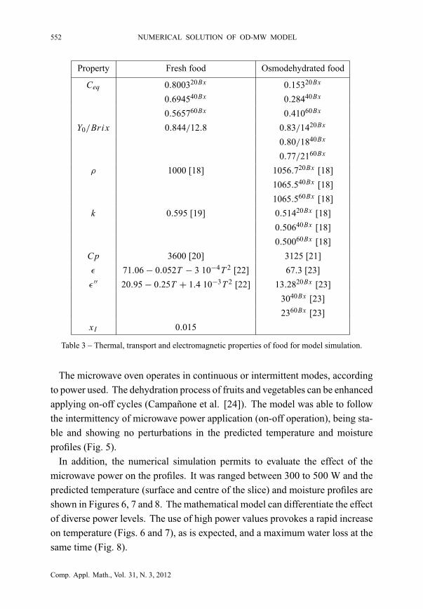
For Step 2 (MWD), Table 3 shows the thermal, transport and electromagneticproperties used as inputs in the runs of the numerical model.

The model allows predict the evolution of temperature and moisture contentduring step 2 (Figs. 4 and 5). OD process applied to pears in sucrose solutionduring two hours was considered as initial condition for this stage. Different ODpre treatments affect the initial water and solute content. The model takes intoaccount this fact varying moisture and solid content of the food (Fig. 4).

The mathematical model shows a good sensibility to the changes of physi-cal properties, due to OD pretreatment. The uptake of solids during OD step,provokes a change of composition of the food material affecting its dielectricproperties (ε′, ε′′), and its ability to interact with radiation (Fig. 5).


“main” — 2012/11/20 — 15:56 — page 552 — #14


Property Fresh food Osmodehydrated food

Ceq 0.800320Bx 0.15320Bx

0.694540Bx 0.28440Bx

0.565760Bx 0.41060Bx

Y0/Bri x 0.844/12.8 0.83/1420Bx

0.80/1840Bx

0.77/2160Bx

ρ 1000 [18] 1056.720Bx [18]

1065.540Bx [18]

1065.560Bx [18]

k 0.595 [19] 0.51420Bx [18]

0.50640Bx [18]

0.50060Bx [18]

Cp 3600 [20] 3125 [21]

ε 71.06 − 0.052T − 3 10−4T 2 [22] 67.3 [23]

ε′′ 20.95 − 0.25T + 1.4 10−3T 2 [22] 13.2820Bx [23]

3040Bx [23]

2360Bx [23]

xI 0.015

Table 3 – Thermal, transport and electromagnetic properties of food for model simulation.

The microwave oven operates in continuous or intermittent modes, accordingto power used. The dehydration process of fruits and vegetables can be enhancedapplying on-off cycles (Campañone et al. [24]). The model was able to followthe intermittency of microwave power application (on-off operation), being sta-ble and showing no perturbations in the predicted temperature and moistureprofiles (Fig. 5).

In addition, the numerical simulation permits to evaluate the effect of themicrowave power on the profiles. It was ranged between 300 to 500 W and thepredicted temperature (surface and centre of the slice) and moisture profiles areshown in Figures 6, 7 and 8. The mathematical model can differentiate the effectof diverse power levels. The use of high power values provokes a rapid increaseon temperature (Figs. 6 and 7), as is expected, and a maximum water loss at thesame time (Fig. 8).


“main” — 2012/11/20 — 15:56 — page 553 — #15


Figure 4 – Predicted moisture content as a function of time for different osmotic pre-

treatments (20, 40 and 60 Brix) when applying microwave power of 500W.

Figure 5 – Predicted temperatures as a function of time for different osmotic pretreat-

ments (20, 40 and 60 Brix) when applying microwave power of 500W.

Finally, the effect of the sample thickness was evaluated in the present work(Figs. 9a and b). The power absorption depends on water content, and then largesamples with high water content absorb more microwave power, increasing theirdehydration rate. This functionality was incorporated in the simulation codes asa Matlab function.


“main” — 2012/11/20 — 15:56 — page 554 — #16


Figure 6 – Simulated thermal histories (surface) applying different microwave power

levels.

Figure 7 – Simulated thermal histories (centre) applying different microwave power

levels.


“main” — 2012/11/20 — 15:56 — page 555 — #17


Figure 8 – Simulated moisture contents applying different microwave power levels.

4 Conclusions

A complete and relatively simple and easy to use mathematical model has beendeveloped for simultaneous prediction of temperature and moisture profiles dur-ing the combined process of osmotic-microwave dehydration. Its main original-ity is that it can consider the initial process of osmotic dehydration and couplethe predicted water and solute concentration profiles to the simultaneous massand energy transfer in the microwave heating step including, also, the inner heatgeneration, the on-off control effect of the microwave oven and different powerlevels. The model considers two numerical techniques to solve differential equa-tions: Runge Kutta (fourth order) for Step 1 and Finite Differences for Step 2.The numerical solution of the balances was implemented in Matlab environmentand it permits to interpret and simulate a technological and industrial process.

From the experimental data and numerical simulations, the effect of the va-riety of food materials, concentration of osmotic solutions, shape and size ofthe product was analyzed during OD process. These food characteristics andoperating conditions affect directly to microwave dehydration during the secondstep, mainly changing the physical properties of the food. Besides microwavepower level and the size of the product was included in the analysis for this step.


“main” — 2012/11/20 — 15:56 — page 556 — #18


Figure 9 – Simulated temperature (a) and moisture contents (b) during MWD for dif-

ferent sample thicknesses.

Finally, we obtained an integrated model that can be used for the prediction ofweight loss in a wide range of operating conditions.


“main” — 2012/11/20 — 15:56 — page 557 — #19


REFERENCES

[1] A.K. Datta and J. Zhang, Porous media approach to heat and mass transfer insolid foods. Department of Agriculture And Biology Engineering, Cornell Uni-versity (1999).

[2] E.A. Spiazzi and R.H. Mascheroni, Modelo de deshidratación osmótica dealimentos vegetales. MAT Serie A, 4 (2001), 23–32.

[3] E.A. Spiazzi and R.H. Mascheroni, Mass transfer model for osmotic dehydrationof fruits and vegetables. I. Development of the simulation model. Journal of FoodEngineering, 34 (1997), 387–410.

[4] C.J. Toupin, M. Marcotte and M. Le Maguer, Osmotically induced mass trans-fer in plant storage tissues: a mathematical model – Part I. Journal of FoodEngineering, 10 (1989), 13–38.

[5] M. Marcotte, C.J. Toupin and M. Le Maguer, Mass transfer in cellular tissues.Part I: The mathematical model. Journal of Food Engineering, 13 (1991), 199–220.

[6] C.H. Tong and D.B. Lund, Microwave heating of baked dough products withsimultaneous heat and moisture transfer. Journal of Food Engineering, 19 (1993),319–339.

[7] H. Ni and A.K. Datta, Moisture as related to heating uniformity in microwaveprocessing of solids foods. Journal of Food Process Engineering, 22 (2002), 367–382.

[8] J.R. Arballo, L.A. Campañone and R.H. Mascheroni, Modelling of microwavedrying of fruits. Drying Technology, 28 (2010), 1178–1184.

[9] Y.E. Lin, R.C. Anantheswaran and V.M. Puri, Finite element analysis of micro-wave heating of solid foods. Journal of Food Engineering, 25 (1995), 85–112.

[10] L.A. Campañone and N.E. Zaritzky, Mathematical analysis of microwave heat-ing process. Journal of Food Engineering, 69 (2005), 359–368.

[11] L. Zhou, V.M. Puri, R.C. Anantheswaran and G. Yeh, Finite element modellingof heat and mass transfer in food materials during microwave heating-model,development and validation. Journal of Food Engineering, 25 (1995), 509–529.

[12] M. Pauli, T. Kayser, G. Adamiuk and W. Wiesbeck, Modeling of mutual couplingbetween electromagnetic and thermal fields in microwave heating. IEEE, 2007(2007), 1983–1986.


“main” — 2012/11/20 — 15:56 — page 558 — #20


[13] R.B. Bird, W.E. Stewart and E.N. Lightfoot, Transport phenomena. John Wileyand Sons, New York (1976).

[14] A. Constantinides and N. Mostoufi, Numerical Methods for Chemical Engineerswith Matlab Applications. Prentice-Hall (1999).

[15] S.C. Chapra and P.P. Canale, Métodos Numéricos para Ingenieros. Fifth Edition.México, Mc Graw-Hill (2007).

[16] L.A. Campañone, V.O. Salvadori and R.H. Mascheroni, Weight loss duringfreezing and storage of unpackaged foods. Journal of Food Engineering, 47 (2001),69–79.

[17] J.A. Arballo, R.R. Bambicha, L.A. Campañone, M.E. Agnelli and R.H. Masche-roni, Mass transfer kinetics and regressional-desirability optimization duringosmotic dehydration of pumpkin, kiwi and pear. International Journal of FoodScience and Technology, 47 (2012), 306–314.

[18] M.E. Agnelli, C.M. Marani and R.H. Mascheroni, Modelling of heat and masstransfer during (osmo) dehydrofreezing of fruits. Journal of Food Engineering, 69(2005), 415–424.

[19] V.E. Sweat, Experimental values of thermal conductivity of selected fruits andvegetables. Journal of Food Science, 39 (1974), 1080–1083.

[20] S.L. Polley, O.P. Snyder and P. Kotnour, A compilation for thermal properties offoods. Food Technology, 34 (1980), 76–94.

[21] A.M. Tocci and R.H. Mascheroni, Determinación por calorimetría diferencial debarrido de la capacidad calorífica y entalpía de frutas parcialmente deshidratadasen soluciones acuosas concentradas de azúcar. In: I Congreso Ibero-Americanode Ingeniería de Alimentos, I (1996), 411–420.

[22] O. Sipahioglu and S.A. Barringer, Dielectric properties of vegetables and fruitsas a function of temperature, ash and moisture content. Journal of Food Science,68 (2003), 234–239.

[23] A.K. Datta and R.C. Anantheswaran, Handbook of Microwave Technology forFood Applications. Marcel Dekker, USA (2001).

[24] L.A. Campañone, Carlos A. Paola and R.H. Mascheroni, Modeling and simula-

tion of microwave heating of foods under different process schedules. Food and

Bioprocess Technology, 5 (2012), 738–749.


numerical solution of coupled mass and energy balances ... · numerical solution of coupled mass...

Documents