numerical simulation of flow inside the square cavity · numerical simulation of flow inside the...

International Journal of Technical Research and Applications e-ISSN: 2320-8163, www.ijtra.com Volume 2, Issue 3 (May-June 2014), PP. 87-94

87 | P a g e

NUMERICAL SIMULATION OF FLOW INSIDE THE SQUARE CAVITY

A. Muthuvel 1, N.Prakash 2, C.Manikandan3 Assistant Professor& J. Godwin John4 Hindustan University 1&2 and EGS Pillay Engineering College, India 3]

[PG scholar Hindustan University 4

Abstract— Numerical simulations have been undertaken for the benchmark problem in a Square cavity by using computational fluid dynamics software. This work aims at discussing the fundamental numerical and computational fluid dynamic aspects which can lead to the definition of the following meshing methods and turbulence models. The meshes used for the simulation are hexahedral, hexahedral cell with near wall refinement, tetrahedral grid, polyhedral, tetrahedral with near wall refinement and polyhedral mesh with prism layer cells based the near wall thickness of Y+ less than one. The turbulence models used for the simulation work are AKN K-Epsilon Low-Re, Realizable K-Epsilon, Realizable K-Epsilon Two-Layer, standard K-Epsilon, standard K-Epsilon Low-Re, Standard K-Epsilon Two-Layer, V2F K-Epsilon, SST(Menter) K-Omega, and Standard(Wilcox) K-Omega. From these meshes and turbulence models, we will conclude the suitable mesh and turbulence for the recirculation flow by the grid independent test. These analytical values of results are compared with reference data which gives an optimization of experimental work. Unsteady simulation was ran for all the Grid Independent mesh with the SST k omega model with the time step of 0.01 sec for 40 seconds. The flow nature is studied with and without the temperature for Reynolds number, 1000 and 10000.

Index Terms— Couette flow, Square Cavity, Mesh, Laminar and Turbulence models, Vortices.

NOMENCLATURE CFD Computational Fluid Dynamics RANS Reynolds Averaged Navier Strokes Equation GIT Grid Independence Test Re Reynolds Number ρ Density µ Dynamic viscosity

I. INTRODUCTION.

Computational fluid dynamics (CFD) is the science of predicting fluid flow, thermal analysis, mass transfer, heat transfer, chemical reactions, and related phenomena by solving the algebraical equations which govern these processes using a numerical process.

CFD is a method to numerically calculate Fluid structure interaction, heat transfer and fluid flow.

Currently, it’s mainly used as an engineering tool to provide data that is complemented to theoretical and reference data. This is mainly the domain of commercially available codes and in-house codes at large companies. CFD can also be used for purely numerical and scientific studies of the fundamentals of turbulence.

From the various sections of CFD, we can analyze the fluid flow. Any experimental work involves high consumption of cost and time. To prevent the wastage of these parameters, we require CFD software. It gives results with experimental input parameters using computer assistance. For this computational analysis of fluid dynamics we use STARCCM+. It is one of the advanced software used for flow analysis. The mean flow equations of mass continuity and momentum equations are inbuilt in this software and are solved numerically.

Experimental studies involves more time and cost to solve. In our studies we create a flow inside the cavity and predict the flow characteristics with various turbulence models. In terms of flow we choose a Couette concept for our studies, which represents to create a velocity at the top wall of the cavity. In this concept of Couette, the side, bottom walls are stationary and top wall should move in the direction of flow. This velocity at the top wall creates vortices inside the cavity.

In our studies we analyze the flow pattern inside the cavity with different meshes and various turbulence models. Initially we have done the geometrical model of the square cavity by using GAMBIT software. After that the model is exported to a suitable STAR-CCM+ file format.

The STAR-CCM+ software helps to run various meshes. The meshed models were initially run for laminar flow conditions for the grid independent test at Re=1000. Based on the grid independent test various turbulence models are validated with the reference results.

II. GEOMETRICAL MODELING

Non dimensional data The geometrical modeling of the square cavity is

shown in Fig 1.Top wall velocity U = 1, Cavity width L = 2, Cavity height H = 2, Reynolds number Re = 1000


88 | P a g e

and Re = 10000, Fluid adimensional density ρ = 1, Fluid adimensional viscosity µ = 2/Re.

Fig.1 geometrical modeling

III. MESH GENERATION

Meshing is a process of discretizing a volume into a

finite set of control volumes or cells. The dicretized domain is called “grid” or “mesh.” The grid is needed because it designates the cells or elements on which the flow is solved.

Fundamentally there are two kinds of meshes available; they are structured and unstructured grid. For this problem structured, unstructured grid and combination of unstructured with structured grid are used for analyzing works and the grid independent meshes are shown in Fig.1 to Fig.8

Let us follow the various types of meshing methods we were used.

1. Rectangular mesh 2. Rectangular with fine wall mesh 3. Triangle mesh 4. Polyhedral mesh 5. Polyhedral with fine wall mesh 6. Tetrahedral with fine wall mesh 7. Prism mesh(rectangle + polyhedral)

Rectangular mesh1:

Fig.2 Structured Grid Rectangular with fine wall mesh2:

Fig.3 Structured grid with near wall refinement Triangle mesh3:

Fig.4 Tetrahedral Grid Polyhedral mesh4:

Fig.5 Polyhedral mesh Polyhedral with fine wall mesh5:

Fig.6 polyhedral mesh with near wall refinement Tetrahedral with fine wall mesh6:


89 | P a g e

Fig. 7 Tetrahedral mesh with near wall

refinement Prism mesh (rectangle + polyhedral)7:

Fig.8 Hybrid mesh These are the various meshes we are used with

different grid sizes. Grid independent test is done for all the meshes. The various grid size geometry results are compared with reference data’s for laminar flow condition.

IV. TURBULENCE MODELS:

A turbulence model is a computational procedure to close the system of mean flow equations. The flow equations are continuity equation and momentum equation, which are solved numerically by various assumptions.

Various scientists develop turbulence models based on assumptions. The k-epsilon and k-omega turbulence models are widely used for industrial applications. In each of these models various assumptions are made to achieve turbulence.

All the turbulence models are based on RANS equation. This equation is a combination of flow and turbulence. The following are the various turbulence models used for the analysis:

K-Epsilon turbulence 1. AKN K-Epsilon low re 2. Realizable K-Epsilon 3. Realizable K-Epsilon two layer 4. Standard K-Epsilon 5. Standard K-Epsilon low re 6. Standard K-Epsilon two layer 7. V2F K-Epsilon

K-Omega turbulence 8. SST (Menter) K-Omega 9. Standard (Wilcox) K-Omega

In this study, the square cavity is assumed to be stationary while the fluid is made to flow inside the cavity at a velocity of 1 m/s as prescribed. The various boundary and operating conditions that are defined in the present study are as follows:

The fluid used for the study is air; hence its density (ρ) is specified as 1 kg/m3. The dynamic viscosity (µ) is calculated from the Reynolds number, length of the cavity, velocity and density.

The inlet boundary is defined as the velocity inlet where a uniform velocity of the fluid is prescribed (1 m/s). Further, the properties that define the turbulence models are also specified at the inlet boundary. The turbulent kinetic energy (k) used in the present study is calculated using the following equation,

…. (1) Where, Ti – turbulent intensity

= 0.0515 J-s/kg-m. For the k-ε models, the dissipation rate (ε) is

specified, which is calculated using the following equation,

... (2) For the k-ω models, specific dissipation rate (ω)

specified for the analysis, is obtained from the following relation,

... (3) The square cavity wall is defined as no-slip wall

with500C temperature and without the temperature to study the effect of various properties at the boundary layer formed on the surface of the cavity except the top wall layer.

Initial iterations are carried out with first-order upwind scheme and under-relaxation factor for velocity as 0.3 and pressure as 0.1 to attain better stability of the solution. Further iterations are carried out with second-order upwind scheme and by increasing the under-relaxation factor of velocity and pressure to 0.5 and 0.3 respectively. This is done to obtain higher accuracy and also to accelerate the convergence. The case is executed till the desired convergence is obtained. The convergence criterion for the problem is 10*e-6.

REFERENCE VALUES: Table 1 U component along vertical midline: Y Re=1000

U Re=10000 U

1.0 1.0 1.0 0.9532 0.65928 0.47221


90 | P a g e

0.9376 0.57492 0.47783 0.9218 0.51117 0.4807 0.9062 0.46604 0.47804 0.7032 0.33304 0.34635 0.4688 0.18719 0.20673 0.2344 0.05702 0.08344 0.0 -0.0608 0.03111 -0.0938 -0.10648 -0.0754 -0.4374 -0.27805 -0.23186 -0.6562 -0.38289 -0.32709 -0.7968 -0.2973 -0.38 -0.8594 -0.2222 -0.41657 -0.8906 -0.18109 -0.42735 -1.0 0.0 0.0 Table 2 V components along horizontal midline: X

Re=1000 V

Re=10000

V 1.0 0.0 0.0 0.9376 -0.21388 -0.54302 0.9218 -0.27669 -0.52987 0.9062 -0.33714 -0.49099 0.8906 -0.39188 -0.45863 0.8126 -0.5155 -0.41496 0.7188 -0.42665 -0.36737 0.6094 -0.31966 -0.30719 0.0 0.02526 0.00831 -0.5312 0.32235 0.27224 -0.5468 0.33075 0.28003 -0.6874 0.37095 0.3507 -0.8124 0.32627 0.41487 -0.8438 0.30353 0.43124 -0.8594 0.29012 0.43733 -0.875 0.27485 0.43983 -1 0.0 0.0

V. RESULT AND DISCUSSION

The steady simulation is carried out for the Reynolds number of 1000 with seven different types of grid to find the grid independent meshes for all the grid types. The steady state simulation is carried out for the various turbulence models like AKN K-Epsilon Low-Re, Realizable K-Epsilon, Realizable K-Epsilon Two-Layer, standard K-Epsilon, standard K-Epsilon Low-Re, Standard K-Epsilon Two-Layer, V2F K-Epsilon, SST(Menter) K-Omega, and Standard(Wilcox) K-Omega with the Reynolds number of 10000 to the grid independent meshes.

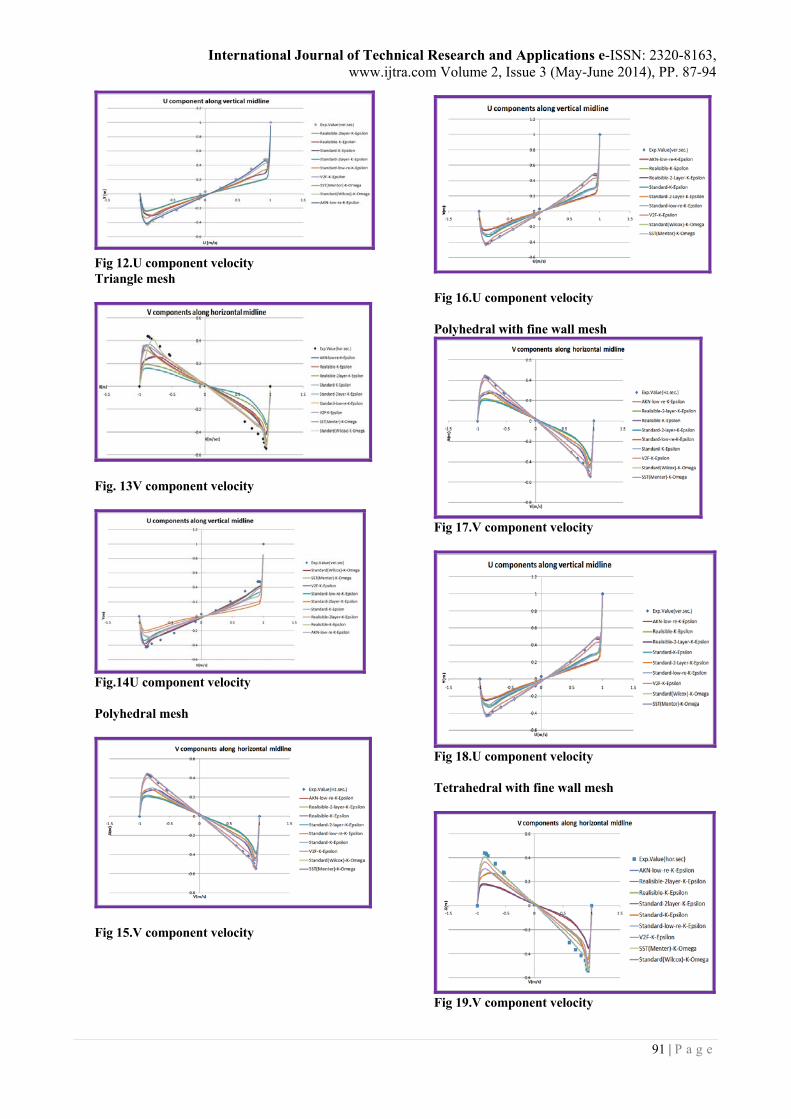
The V component velocity and U component velocity in horizontal midline and vertical midline for various turbulence models are shown in Fig from 9 to 22.

SST K-Omega turbulence model predicts the component velocity nicely with reference values for all the grid is shown in Fig from 23 and 24.Polyhedral cells with near wall refinement and hexahedral cell with near wall refinement meshes predicts the reference data nicely as shown in Fig.25 and 26.

The unsteady simulation is carried out for polyhedral cells with near wall refinement and hexahedral cell with near wall refinement meshes for the Reynolds number of 10000 with SST K omega turbulence model. The velocity stream lines for various time steps are shown in Fig.27 to 32.

Rectangular mesh

Fig 9.V component velocity

Fig 10.U component velocity Rectangular with fine wall mesh



91 | P a g e

Fig 12.U component velocity Triangle mesh

Fig. 13V component velocity

Fig.14U component velocity Polyhedral mesh


Fig 16.U component velocity Polyhedral with fine wall mesh


Fig 18.U component velocity Tetrahedral with fine wall mesh



92 | P a g e

Fig 20.U component velocity Prism mesh (rectangle + polyhedral)


Fig 22.U component velocity

Fig 23- Best Mesh in Horizontal Section

’ Fig 24- Best Mesh in vertical Section

Fig 25-Best mesh in Horizontal direction

Fig 26-Best mesh in Vertical direction For Polyhedral with fine wall mesh For1 sec,

Fig.27 Velocity stream lines


93 | P a g e

For 2 sec,

Fig.28 Velocity stream lines For 6 sec,

Fig.29 Velocity stream lines For 10 sec

Fig.30 Velocity stream lines For 15 sec

Fig.31 Velocity stream lines For 20 sec,

Fig.32 Velocity stream lines

VI. CONCLUSION:

The simulation is carried out for various types of grid with different grid ratios realizable K epsilon turbulence model for find the grid independent mesh.

Polyhedral cells with near wall refinement and hexahedral cell with near wall refinement meshes agrees with the reference results for Reynolds number of 1000 and 10000.

SST (Menter) K-Omega turbulence model predict the component velocity nicely with the reference values for Reynolds number of 10000 with and without the temperature effect.

REFERENCES

[1] G. BARAKOS AND E. MITSOULIS*,”1994 Department of Chemical Engineering, University of Ottawa, Ottawa, Ont. KIN 6N5, Canada and D. ASSIMACOPOULOS Section II, Department of Chemical Engineering, National Technical University of Athens, Athens 157-73, Greece,” LAMINAR AND TURBULENT MODELS WITH WALL FUNCTIONS,” INTERNATIONAL JOURNAL FOR NUMERICAL METHODS IN FLUIDS, VOL. 18, 695-719

[2] c.shu & k. h. a. wee department of mechanical and production engineering, national university of Singapore 119260,” Numerical simulation of natural convection in a square cavity by simple- generalized differential quadrature method,” computers and fluids 31 (2002) 209-226

[3] Jun chang,” department of computer science,” university of kentucky, 773 anderson hall, lexington, KY 40506-0046, USA, april 6, 2000,”2D square driven cavity using fourth order compact finite difference schemes,”

[4] .N. Dixit, V. Babu * Thermodynamics and Combustion Engineering Laboratory, Department of Mechanical Engineering, Indian Institute of Technology Madras, Chennai 600 036, India,” high Rayleigh number natural convection in a square cavity using the lattice Boltzmann method,” July 2005

[5] M. RASHID1, A.B.M.A. KAISH2, M.M. ISLAM1 AND M.T. ISLAM1 1Deparment of Mathematics and Physics, Faculty of Computer Science and Technology, Hajee Mohammad Danesh Science and Technology University, Dinajpur, Bangladesh; 2Graduate Student, Dept. of Civil & Structural Engineering, National University of Malaysia. INCOMPRESSIBLE FLOWS IN ONE-SIDED LID-DRIVEN SQUARE CAVITY BY FINITE ELEMENT METHOD,” Strategy 5(3):114-119(December 2011)

[6] M. RASHID1, A.B.M.A. KAISH2 AND M.M. ISLAM1

1Deparment of Mathematics and Physics, Faculty of Computer Science and Technology, Hajee Mohammad Danesh Science and Technology University, Dinajpur, Bangladesh; 2Graduate Student, Dept. of Civil & Structural Engineering, National University of Malaysia.


94 | P a g e

,” TURBULENT FLOWS IN TWO-SIDED LID-DRIVEN SQUARE CAVITY BY FINITE ELEMENT METHOD,”Strategy 5(3):120-124(December 2011)

[7] GAMBIT, user guide, copyright 1988-2013, http://www.fluent.com.

[8] STAR-CCM+ userguide, Star-ccm+ v6.02, 2011, http://www.cd-adapco.com.

numerical simulation of flow inside the square cavity · numerical simulation of flow inside the...

Documents