numerical methods for pdes fem - abstract formulation, the ...€¦ · fem - abstract formulation,...

Platzhalter für Bild, Bild auf Titelfolie hinter das Logo einsetzen

Dr. Noemi Friedman

Numerical methods for PDEs FEM - abstract formulation, the Galerkin method

Galerkin method | Dr. Noemi Friedman | PDE2 tutorial | Seite 2

Contents of the course

• Fundamentals of functional analysis • Abstract formulation FEM • Application to conrete formulations • Convergence, regularity • Variational crimes • Implementation • Mixed formulations (e.g. Stokes) • Stabilisation for flow problems • Error indicators/estimation • Adaptivity

Galerkin method | Dr. Noemi Friedman | PDE2 tutorial | Seite 3

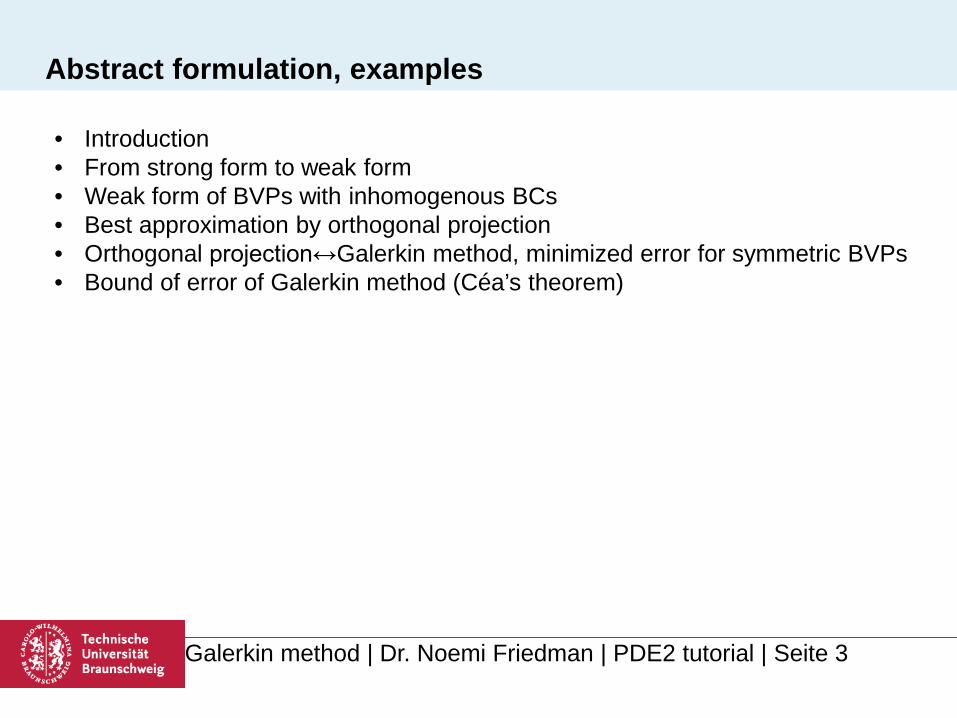
Abstract formulation, examples

• Introduction • From strong form to weak form • Weak form of BVPs with inhomogenous BCs • Best approximation by orthogonal projection • Orthogonal projection↔Galerkin method, minimized error for symmetric BVPs • Bound of error of Galerkin method (Céa’s theorem)

Galerkin method| Dr. Noemi Friedman | PDE tutorial | Seite 4

Introduction to Galerkin method

Matlab code from Gockenbach book: http://www.math.mtu.edu/~msgocken/fembook Equations followed throughout the semester [Chapter1]: Laplace/Poisson equation: • bar with uniaxial load • steady state heat flow • small vertical deflections of a membrane • stationary heat equation Other ellptic BVPs: • isotropic elasticity

http://www.math.mtu.edu/~msgocken/fembook







| Dr. Noemi Friedman | PDE tutorial | Seite 5

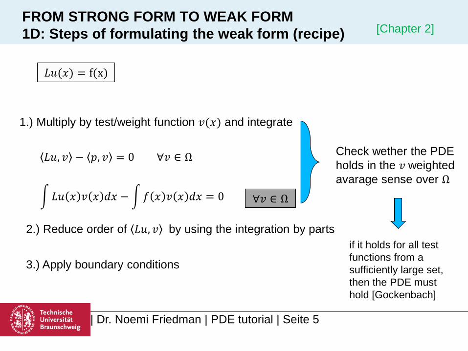
FROM STRONG FORM TO WEAK FORM 1D: Steps of formulating the weak form (recipe)

𝐿𝐿, 𝑣 − 𝑝, 𝑣 = 0 ∀𝑣 ∈ Ω

1.) Multiply by test/weight function 𝑣(𝑥) and integrate

𝐿𝐿(𝑥) = f(x)

�𝐿𝐿 𝑥 𝑣 𝑥 𝑑𝑥 − �𝑓 𝑥 𝑣 𝑥 𝑑𝑥 = 0

2.) Reduce order of 𝐿𝐿, 𝑣 by using the integration by parts

3.) Apply boundary conditions

∀𝑣 ∈ Ω

Check wether the PDE holds in the 𝑣 weighted avarage sense over Ω

if it holds for all test functions from a sufficiently large set, then the PDE must hold [Gockenbach]

[Chapter 2]

17. 01. 2014. | Dr. Noemi Friedman | PDE tutorial | Seite 6

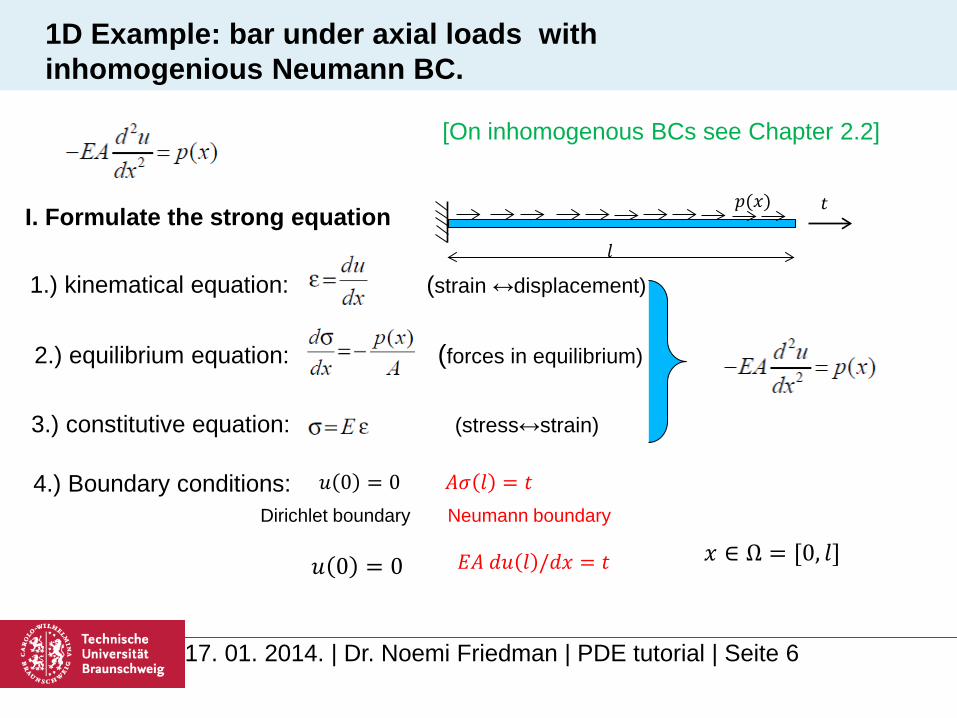
1D Example: bar under axial loads with inhomogenious Neumann BC.

1.) kinematical equation: (strain ↔displacement)

2.) equilibrium equation: (forces in equilibrium)

3.) constitutive equation: (stress↔strain)

4.) Boundary conditions:

I. Formulate the strong equation 𝑝(𝑥)

𝑙

𝑥 ∈ Ω = [0, 𝑙]

𝑡

𝐿 0 = 0

𝐸𝐸 𝑑𝐿 𝑙 /𝑑𝑥 = 𝑡

𝐸𝐴 𝑙 = 𝑡 Neumann boundary Dirichlet boundary

𝐿 0 = 0

[On inhomogenous BCs see Chapter 2.2]

| Dr. Noemi Friedman | PDE tutorial | Seite 7

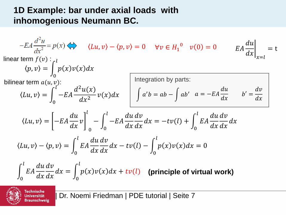
1D Example: bar under axial loads with inhomogenious Neumann BC.

(principle of virtual work)

Integration by parts:

𝐿𝐿, 𝑣 − 𝑝, 𝑣 = 0 ∀𝑣 ∈ 𝐻10

𝑝, 𝑣 = � 𝑝 𝑥 𝑣 𝑥 𝑑𝑥𝑙

0

𝐿𝐿, 𝑣 = � −𝐸𝐸𝑑2𝐿(𝑥)𝑑𝑥2 𝑣(𝑥)𝑑𝑥

𝑙

0 𝑏𝑏 =

𝑑𝑣𝑑𝑥

𝐿𝐿, 𝑣 = −𝐸𝐸𝑑𝐿𝑑𝑥 𝑣

𝑙

0− � −𝐸𝐸

𝑑𝐿𝑑𝑥

𝑑𝑣𝑑𝑥 𝑑𝑥

𝑙

0= −𝑡𝑣(𝑙) + � 𝐸𝐸

𝑑𝐿𝑑𝑥


𝑙

0

𝑣 0 = 0

𝐿𝐿, 𝑣 − 𝑝, 𝑣 = � 𝐸𝐸𝑑𝐿𝑑𝑥


𝑙

0− 𝑡𝑣 𝑙 − � 𝑝 𝑥 𝑣 𝑥 𝑑𝑥

𝑙

0= 0

� 𝐸𝐸𝑑𝐿𝑑𝑥


𝑙

0= � 𝑝 𝑥 𝑣 𝑥 𝑑𝑥

𝑙

0+ 𝑡𝑣(𝑙)

𝑎 = −𝐸𝐸𝑑𝐿𝑑𝑥

�𝑎′𝑏 = 𝑎𝑏 − �𝑎𝑏′

linear term 𝑓(𝑣) :

bilinear term 𝑎(𝐿,𝑣):

𝐸𝐸𝑑𝐿𝑑𝑥�𝑥=𝑙

= t

. | Dr. Noemi Friedman | PDE tutorial | Seite 8

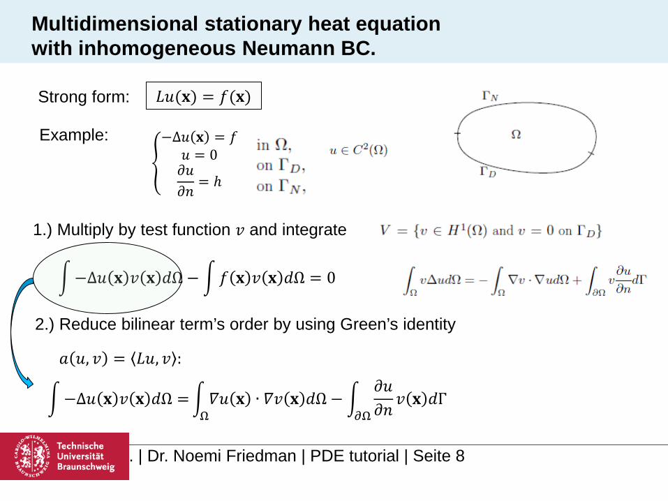
Multidimensional stationary heat equation with inhomogeneous Neumann BC.

𝐿𝐿(𝐱) = 𝑓(𝐱) Strong form:

Example:

1.) Multiply by test function 𝑣 and integrate

�−Δ𝐿 𝐱 𝑣 𝐱 𝑑Ω − �𝑓 𝐱 𝑣 𝐱 𝑑Ω = 0

�−Δ𝐿 𝐱 𝑣 𝐱 𝑑Ω =�𝛻𝐿 𝐱 ∙ 𝛻𝑣 𝐱 𝑑Ω

Ω− �

𝜕𝐿𝜕𝑛 𝑣 𝐱 𝑑Γ

𝜕Ω

2.) Reduce bilinear term’s order by using Green’s identity

�

−Δ𝐿 𝐱 = 𝑓𝐿 = 0𝜕𝐿𝜕𝑛

= ℎ

𝑎 𝐿, 𝑣 = 𝐿𝐿, 𝑣 :


Multidimensional stationary heat equation with inhomogeneous Neumann BC.


Ω− �

𝜕𝐿𝜕𝑛

𝑣 𝐱 𝑑Γ

𝜕Ω


�𝜕𝐿𝜕𝑛

𝑣 𝐱 𝑑Γ = �𝜕𝐿𝜕𝑛

𝑣 𝐱 𝑑Γ +

Γ𝑁�

𝜕𝐿𝜕𝑛

𝑣 𝐱 𝑑Γ = � ℎ𝑣 𝐱 𝑑Γ

Γ𝑁

Γ𝐷

𝜕Ω

ℎ 0


Ω− � ℎ𝑣 𝐱 𝑑Γ

Γ𝑁

�𝛻𝐿 𝐱 ∙ 𝛻𝑣 𝐱 𝑑Ω

Ω= � 𝑓 𝐱 𝑣 𝐱 𝑑Ω + � ℎ𝑣 𝐱 𝑑Γ

Γ𝑁

Ω


Multidimensional stationary heat equation with inhomogeneous Dirichlet and Neumann BC.

𝐿𝐿(𝐱) = 𝑓(𝐱) Strong form:

Example:

1.) Multiply by test function 𝑣 and integrate

�−Δ𝐿 𝐱 𝑣 𝐱 𝑑Ω − �𝑓 𝐱 𝑣 𝐱 𝑑Ω = 0


Ω− �

𝜕𝐿𝜕𝑛 𝑣 𝐱 𝑑Γ

𝜕Ω

2.) Reduce order of 𝐿𝐿, 𝑣 by using divergence theoreem

−Δ𝐿 𝐱 = 𝑓𝐿 = 𝑔𝜕𝐿𝜕𝑛

= ℎ

convert to homogeneous problem:

𝐿 = 𝜔 + 𝐿� 𝜔:known function,𝜔 = 𝑔 on Γ𝐷 𝐿�:new function that we look for


Multidimensional stationary heat equation with inhomogeneous Dirichlet and Neumann BC.

�𝛻𝐿 𝐱 ∙ 𝛻𝑣 𝐱 𝑑Ω


Γ𝑁

Ω


Ω− �

𝜕𝐿𝜕𝑛

𝑣 𝐱 𝑑Γ

𝜕Ω


�𝜕𝐿𝜕𝑛

𝑣 𝐱 𝑑Γ = �𝜕𝐿𝜕𝑛

𝑣 𝐱 𝑑Γ +

Γ𝑁�

𝜕𝐿𝜕𝑛

𝑣 𝐱 𝑑Γ = � ℎ𝑣 𝐱 𝑑Γ

Γ𝑁

Γ𝐷

𝜕Ω

ℎ 0

�𝛻 𝜔 𝐱 + 𝐿� 𝐱 ∙ 𝛻𝑣 𝐱 𝑑Ω


Γ𝑁

Ω

∫ 𝛻𝐿� 𝐱 ∙ 𝛻𝑣 𝐱 𝑑Ω Ω = ∫ 𝑓 𝐱 𝑣 𝐱 𝑑Ω + ∫ ℎ𝑣 𝐱 𝑑Γ

Γ𝑁 Ω − ∫ 𝛻𝜔 𝐱 ∙ 𝛻𝑣 𝐱 𝑑Ω

Ω

from natural/Neumann BC from essential/Dirichlet BC


Existence and uniqueness of the solution of BVPs

𝐿𝐿(𝐱) = 𝑓(𝐱) 𝐿𝐿, 𝑣 = 𝑓, 𝑣 ∀𝑣 ∈?

Strong form: Weak form:

Does the solution exists? Does it have a unique solution?

𝐿 ∈? 𝑎(𝐿, 𝑣) 𝐹(𝑣)

bilinear term linear term

In accordance to the Lax-Milgram Lemma if: F(∙) bounded, linear functional a ∙,∙ bounded, V-elliptic bilinear functional and V a Hilbert space

• solution 𝐿 exists • unique solution 𝐿 ∈ 𝑉 • +solution 𝐿 depends

continiously on 𝑓 For a specific BVP one has to find the right Hilbert space (Sobolev space or L2 space) where the conditions for a ∙,∙ and F(∙) are satisfied, and then we know, that in that space we have a unique solution!

[Chapter 2.4]


Existence and uniqueness of the solution of BVPs ─ examples

• unique solution 𝐿 ∈ 𝐻01

• 𝑣 ∈ 𝐻01

1. Poisson equation: F(∙) linear functional, in 𝐻0

1: bounded a ∙,∙ bilinear functional, in 𝐻0

1: bounded, V-elliptic a ∙,∙ bilinear functional, in 𝐿2: not bounded a ∙,∙ bilinear functional, in 𝐻1: not V-elliptic 2. Plate equation F(∙) linear functional, in 𝐻𝐸

2: bounded a ∙,∙ bilinear functional, in 𝐻𝐸

2: bounded, V-elliptic

−Δ𝐿 𝐱 = 𝑓 𝐱 F(𝑣) = ∫𝑓 𝐱 𝑣 𝐱 𝒅𝐱

a ∙,∙ = �𝛻𝐿 𝐱 𝛻𝑣 𝐱 𝒅𝐱

we have to narrow down the space in which we look for the solution, because we can not prove that there is a unique solution in L2 or in H1

−ΔΔ𝐿 𝐱 = 𝑓 𝐱 F(𝑣) = ∫𝑓 𝐱 𝑣 𝐱 𝒅𝐱

a ∙,∙ = �Δ𝐿 𝐱 Δ𝑣 𝐱 𝒅𝐱

• unique solution 𝐿 ∈ 𝐻𝐸2

• 𝑣 ∈ 𝐻𝐸2


Proxi model – projection of the solution Let’s say we know that there is a unique solution in 𝑉 = 𝐻0

1. But 𝑉 is an infinite dimensional space Let’s narrow down the space, where we are trying to find the solution, to a finite dimensional space example: instead of finding 𝐿(𝑥) ∈ 𝐻0

1 we try to find the coefficients 𝛼𝑗 of a „proxi model” (ansatz function):

𝐿ℎ 𝑥 = �𝛼𝑗𝜔𝑗

𝑛

𝑗=1

(𝑥)

where 𝜔𝑗 x : known (linearly independent) basis or ansatz functions 𝐿ℎ 𝑥 : the approximation of the solution 𝐿(𝑥), which is in an n-dimensional space: 𝐿ℎ ∈ 𝑉ℎ = span{𝜔1,𝜔2, …𝜔𝑛}

[Chapter 3]


Proxi model – projection of the solution Let’s fix this subspace to a specific 𝑉ℎ (that is, we fix the ansatz functions in our examples) How do we get the best approximation of the solution in this space from the equation: Our goal is to minimize the difference in between the solution and the approximation: error = 𝐿 𝐱 − 𝐿ℎ 𝐱 < 𝐿 𝐱 − z 𝐱 ∀z 𝐱 ∈ 𝑉ℎ The best approximation 𝐿ℎ to 𝐿 from 𝑉ℎ is the one where the error is orthogonal to the space of 𝑉ℎ, that is to all possible z 𝐱 ∈ 𝑉ℎ. Instead of writing it for all z (as z is an n-dimensional space) we can write ∀𝜔𝑖 𝑖 = 1. .𝑛

𝐿 𝐱 − 𝐿ℎ 𝐱 ,𝜔𝑖 𝐱 = 0 𝑖 = 1. .𝑛

𝐿𝐿(𝐱) = 𝑓(𝐱)

Best approximation to 𝐿 𝐱 from 𝑉ℎ


Proxi model – projection of the solution Plugging in the proxi model to the orthogonality condition we have: Rearranging the equation we get:

𝐿,𝜔𝑖 −�𝛼𝑗

𝑛

𝑗=1

𝜔𝑗 ,𝜔𝑖 = 0 𝑖 = 1. . 𝑛

�𝛼𝑗

𝑛

𝑗=1

𝜔𝑗 ,𝜔𝑖 = 𝐿,𝜔𝑖 𝑖 = 1. .𝑛

𝐿 −�𝛼𝑗𝜔𝑗

𝑛

𝑗=1

,𝜔𝑖 = 0 𝑖 = 1. .𝑛

𝐺𝑖𝑗

�𝛼𝑗

𝑛

𝑗=1

𝐺𝑖𝑗 = 𝑏𝑗 𝐆𝜶 = 𝐛

𝑏𝑗


Proxi model – projection of the solution where 𝐺𝑖𝑗 = 𝜔𝑗 ,𝜔𝑖 : can be calculated from the basis functions and the inner product

of the given space (if the basis is orthonormal the matrix is the identity matrix

𝑏𝑗 = 𝐿,𝜔𝑖 : ? 𝛼𝑗: The coefficients that we are looking for But how do we get 𝑏𝑗 = 𝐿,𝜔𝑖 ? We know If the left hand side of the weak equation is a V-elliptic, bounded bilinear functional, that is also symmetric, then it can be written as:

𝐿𝐿, 𝑣 𝐿2 = 𝑎(𝐿, 𝑣) = 𝐿, 𝑣 𝐸

𝐆𝜶 = 𝐛

𝐿𝐿, 𝑣 𝐿2 = 𝑓, 𝑣 𝐿2


Proxi model – projection of the solution That means that with Galerkin method we orthogonalize the projection, that is, we minimize the error in the energy space. And the matrix equation, that we can calculate the coefficients from, will have the form: with

𝐺𝑖𝑗 = 𝜔𝑗 ,𝜔𝑖 𝐸= 𝑎(𝜔𝑗,𝜔𝑖)

𝑏𝑗 = 𝐿,𝜔𝑖 𝐸 = 𝑓,𝜔𝑖 𝐿2

Example: 𝑥 = 0, 𝑙 , 𝐿 0 = 0, 𝐿 𝑙 = 0

𝐿𝐿 = −𝐸𝐸𝜕2𝐿(𝑥)𝜕2𝑥 𝑓 = 𝑝

𝐺𝑖𝑗 = 𝜔𝑗(𝑥),𝜔𝑖(𝑥)𝐸

= � 𝐸𝐸𝑑𝜔𝑗(𝑥)𝑑𝑥

𝑑𝜔𝑖(𝑥)𝑑𝑥 𝑑𝑥

𝑙

0 𝑏𝑗 = 𝑓,𝜔𝑖 𝐿2 = � 𝑝 𝑥 𝜔𝑖 𝑥 𝑑𝑥

𝑙

0

𝐆𝜶 = 𝐛


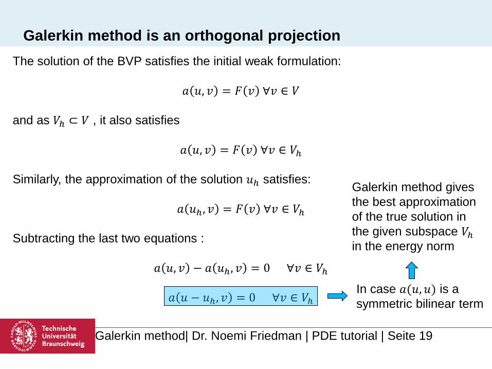
Galerkin method is an orthogonal projection The solution of the BVP satisfies the initial weak formulation:

𝑎 𝐿, 𝑣 = 𝐹 𝑣 ∀𝑣 ∈ 𝑉 and as 𝑉ℎ ⊂ 𝑉 , it also satisfies

𝑎 𝐿, 𝑣 = 𝐹 𝑣 ∀𝑣 ∈ 𝑉ℎ Similarly, the approximation of the solution 𝐿ℎ satisfies:

𝑎 𝐿ℎ , 𝑣 = 𝐹 𝑣 ∀𝑣 ∈ 𝑉ℎ Subtracting the last two equations :

𝑎 𝐿, 𝑣 − 𝑎 𝐿ℎ, 𝑣 = 0 ∀𝑣 ∈ 𝑉ℎ

𝑎 𝐿 − 𝐿ℎ, 𝑣 = 0 ∀𝑣 ∈ 𝑉ℎ

Galerkin method gives the best approximation of the true solution in the given subspace 𝑉ℎ in the energy norm

In case 𝑎(𝐿,𝐿) is a symmetric bilinear term


Céa’s theorem Conclusion from before: 𝑎 ⋅,⋅ : symmetric Gallerkin method gives the best approximation in the

energy norm But what about the error in other norms? According to Céa’s theorem (see prove at the lecture note), even without 𝑎 ⋅,⋅ being symmetric, the error of the approximation of Galerkin will be allways bounded:

𝐿 − 𝐿ℎ ≤𝑀𝛿 𝐿 − 𝑣 ∀𝑣 ∈ 𝑉ℎ

Where 𝑀 and 𝛿 are constants from the conditions of boundedness and V-ellipticity of the bilinear term 𝑎 ⋅,⋅ :

𝑎 𝐿, 𝑣 ≤ 𝑀 𝐿 𝑣 𝑎 𝐿,𝐿 ≥ 𝛿 𝐿 2

and 𝐿 − 𝑣 is the norm of the difference in between the true solution and any 𝑣 ∈ 𝑉ℎ This term depends on the n-dimensional space 𝑉ℎ chosen, and the space where the true solution lies in.

numerical methods for pdes fem - abstract formulation, the ...€¦ · fem - abstract formulation,...

Documents