numerical issues in threshold autoregressive modeling of time series
TRANSCRIPT
Journal of Economic Dynamics & Control 27 (2003) 2219–2242www.elsevier.com/locate/econbase
Numerical issues in threshold autoregressivemodeling of time series
Jerry Coakleya ;∗, Ana-Mar,-a Fuertesb, Mar,-a-Teresa P,erezcaDepartment of Accounting, Finance and Management, University of Essex, Wivenhoe Park,
Colchester CO4 3SQ, UKbFaculty of Finance, Cass Business School, UK
cDepartmento de Matem'atica Aplicada, ETSII, University of Valladolid, Spain
Abstract
This paper analyses the contribution of various numerical approaches to making the estimationof threshold autoregressive time series more e3cient. It relies on the computational advantagesof QR factorizations and proposes Givens transformations to update these factors for sequentialLS problems. By showing that the residual sum of squares is a continuous rational functionover threshold intervals it develops a new <tting method based on rational interpolation and thestandard necessary optimality condition. Taking as benchmark a simple grid search, the paperillustrates via Monte Carlo simulations the e3ciency gains of the proposed tools.? 2002 Elsevier Science B.V. All rights reserved.
JEL classi-cation: C63; C51; C61
Keywords: Band-TAR; QR factorization; Givens rotations; Rational interpolation
1. Introduction
Nonlinear models have been widely applied in recent years to capture asymmetries,limit cycles and jump phenomena in the behavior of economic and <nancial time series.Among these models, the threshold autoregression (TAR) introduced by Tong and Lim(1980) has received particular attention. This is perhaps the simplest generalizationof an AR model which allows for diCerent regimes for the series depending on itspast values. TAR models have been successfully applied to model nonlinearities in<nancial variables by permitting an inner regime of sluggish adjustment for small
∗ Corresponding author. Tel.: +44-0207-631-6418; fax: +44-0207-631-641.E-mail address: [email protected] (J. Coakley).
0165-1889/02/$ - see front matter ? 2002 Elsevier Science B.V. All rights reserved.PII: S0165 -1889(02)00123 -9
2220 J. Coakley et al. / Journal of Economic Dynamics & Control 27 (2003) 2219–2242
disequilibria— or small deviations from some long run equilibrium path or attractor—and mean reversion in an outer regime comprising large deviations. This nonlinearbehavior has been rationalized on the basis of transaction costs or a low signal-to-noiseratio hindering pro<table arbitrage opportunities for small disequilibria.TAR models have also been used successfully to explore asymmetries in macro-
economic variables over the course of the business cycle. 1 There is the question ofwhether the apparent persistence in a economic time series such as GNP or unemploy-ment provides evidence of asymmetries that standard Gaussian linear (<xed) parametermodels cannot accommodate. Thus one aspect of this literature relates to proposalsfor new unit root tests in a TAR framework—which can be thought of as extensionsof existing linear tests—where the alternative hypothesis is stationarity with possi-ble asymmetric adjustment (Enders and Granger, 1998; Berben and van Dijk, 1999;Coakley and Fuertes, 2001a, b).A practical problem in using TARs is that standard maximum likelihood (ML)
estimation algorithms cannot be applied since the log-likelihood function is not con-tinuously diCerentiable with respect to the threshold parameter. This problem has beencommonly tackled by implementing a grid search (GS) over a feasible region of thethreshold space. For a given threshold value, the TAR model is piecewise linear inthe remaining parameters and thus linear estimation techniques can be applied. Thethreshold value that maximizes the log-likelihood function over the grid is the MLestimate. Since in principle any point in the continuous threshold space could maxi-mize the log-likelihood, a full or detailed GS with a small step size is preferable to aGS restricted to the order statistics of the threshold variable.While the latter may deliver inaccurate model parameter estimates for small sample
sizes, a practical problem with the detailed GS is that it may prove computationallyexpensive and especially so for widely dispersed data. Though computation costs maynot be an issue in ad hoc <tting of TAR models to single time series, these becomerelevant in inference applications of TARs using simulation techniques. For instance,exploring the small sample properties of TAR-based tests by Monte Carlo or bootstrapsimulation methods and/or estimating response surfaces with a sensible number ofreplications can become intractable if no attention is paid to estimation time. Theseproblems are aggravated if the model is nonlinear in more than one parameter whicheCectively implies a high-dimensional grid search.The purpose of this paper is twofold. First, it explores systematically the value-added
of QR factorizations and Givens transformations in TAR <tting. In this sense it seeksto <ll an existing gap in investigating numerical aspects of TAR modeling and to pro-vide practical recommendations. Second, by showing that the residual sum of squaresof a certain class of TARs is a continuous rational function over threshold intervals,it proposes a novel <tting approach. Its main advantage is allowing for a continu-ous feasible range for the threshold parameter. Our approach can be considered as
1 For instance, TARs have been applied to explore the term structure of interest rates by Endersand Granger (1998), the Nelson–Plosser data set by Rothman (1999), unemployment behavior by Caner andHansen (1998) and Coakley et al. (2002), and to model US output by Pesaran and Potter (1997) andKapetanios (1999a).
J. Coakley et al. / Journal of Economic Dynamics & Control 27 (2003) 2219–2242 2221
equivalent to a grid search in the limit as the step size becomes increasingly small,while still remaining computationally tractable in contrast to the latter.The remainder of the paper is organized as follows. In Section 2 we outline the TAR
framework and estimation issues. In Section 3 we discuss some numerical tools andcombine them in a novel <tting approach which is summarized step-by-step. The proofsof Proposition 1 and Theorems 2 and 3 are deferred to an appendix. In Section 4 weevaluate via Monte Carlo simulation the e3ciency gains of these tools and concludein Section 5.
2. The model
2.1. Band-TAR dynamics
An m-regime TAR model can be written as
zt =m∑j=1
(�j0 + �j
1zt−1 + · · ·+ �jpj zt−pj)It(
j−16 vt−d ¡ j) + t ; (1)
where t ∼ nid(0; �2); It(·) is the indicator function, −∞= 0¡ 1¡ · · ·¡ m=∞are threshold parameters, pj and d are the positive integer-valued autoregressive (AR)lag order and threshold delay, respectively. This is a nonlinear model in time butpiecewise linear in the threshold space �. More speci<cally, (1) is a discontinuous (inconditional-mean) TAR which partitions the one-dimensional Euclidean space into mlinear AR regimes. The speci<c linear mechanism at any given point in time dependson the values taken by the threshold or switching variable vt−d. The resulting modelfor vt−d=zt−d is sometimes called a self-exciting TAR (SETAR) to distinguish it fromthose models where vt−d is exogenous. 2
Consider the following <rst-diCerence reparameterization of (1) for m= 3:
Pzt = A(t; )−It(vt−d ¡− ) + B(t)It(−6 vt−d6 )
+A(t; )+It(vt−d ¿) + t (2)
with
A(t; )− = �1(zt−1 + ) + �2(zt−2 + ) + · · ·+ �p(zt−p + );
A(t; )+ = �1(zt−1 − ) + �2(zt−2 − ) + · · ·+ �p(zt−p − );
B(t) = �0 + �1zt−1 + �2zt−2 + · · ·+ �qzt−q;
where ¿ 0 is an identifying restriction. This is a generalization of the Band-SETARmodel introduced by Balke and Fomby (1997) where p= q=1 and �0 = �1 = 0. Thelatter implies random walk behavior in the inner band. An important feature of
2 (SE)TAR models are special cases of Priestley’s (1998) general nonlinear state-dependent models. In therelated smooth transition AR (STAR) class of models It(·) is replaced by a (continuous) smooth function.See Tong (1983) and Granger and TerRasvirta (1993).
2222 J. Coakley et al. / Journal of Economic Dynamics & Control 27 (2003) 2219–2242
Band-TAR processes is that their stability properties depend on the outer band dynamicsonly. More speci<cally, even when the inner band has unit root/explosive behavior, ifthe roots of the outer band characteristic equation Lp−(�1+1)Lp−1−�2Lp−2−· · ·−�p=0lie within the complex unit circle then, whenever |vt−d|¿; zt converges to the edgesof the band [− ; ] which act as attractors, and is stationary overall. This Band-TARscheme has been extensively applied in the recent nonlinear literature to analyse thebehavior of (demeaned) <nancial and economic variables which are expected to exhibitsymmetric change-point dynamics around a long run equilibrium path. 3
A straightforward extension of (2) is an asymmetric Band-TAR with adjustmentparameters �uj ; j = 1; : : : ; pu and �lj; j = 1; : : : ; pl for the upper (vt−d ¿ u) and lower(vt−d6 − l) outer regimes, respectively. Another important related speci<cation isthe following continuous (C-)TAR:
Pzt = �u1(zt−1 − )It + �l1(zt−1 − )(1− It) +p∑j=1
�jPzt−j + t ;
It =
{1 if vt−1¿ 0;
0 otherwise;(3)
where vt−1 = zt−1 − . This model characterizes a process with possibly asymmetricadjustment (�u1 �= �l1) towards the attractor . Note that a common feature of (2) and(3) is that appears explicitly in the conditional mean of Pzt . This C-TAR classof models—which has generated an extensive literature 4 —was formally introduced byChan and Tsay (1998) and proposed by Enders and Granger (1998) as a generalizationof the linear augmented Dickey–Fuller regression to test for unit root dynamics.
2.2. The estimation problem
Let {zt}Nt=1 and {vt}Nt=1 be the time series available for estimation of (2). Ordinary LSor, equivalently, conditional ML under Gaussian innovations, lead to the minimizationof the following residual sum of squares (RSS) function:
RSS(�) =n∑t
(Pzt − A(t; )−)2It(vt−d ¡− ) +n∑t
(Pzt − B(t))2It(|vt−d|6 )
+n∑t
(Pzt − A(t; )+)2It(vt−d ¿)
3 Note that (2) assumes outer regimes with the same dynamics �(L) and symmetric thresholds withrespect to zero. For instance, Coakley and Fuertes (2001c) employ this symmetric model to explore theissue of market segmentation in Europe while Obstfeld and Taylor (1997) <t a more restrictive version with�0 = �1 = · · · = �q = 0 to analyse the PPP hypothesis.
4 For example, Berben and van Dijk (1999) develop a unit root test based on (3) and Coakley and Fuertes(2000) extend (3) to develop tests for AR mean-reversion against sign and amplitude asymmetric adjustment.
J. Coakley et al. / Journal of Economic Dynamics & Control 27 (2003) 2219–2242 2223
with respect to �=(; �′; �′; d; p; q)′, where �=(�1; : : : ; �p)′ and �=(�0; �1; : : : ; �q)′ arethe outer and inner AR parameters, respectively, and n=N −max(d; p; q) the eCectivesample size.Let us assume that the lags (d; p; q) are known a priori. Our goal is to estimate the
remaining parameters ; � and �. Since the above objective function is discontinuousin , standard gradient-based algorithms cannot be applied. If the threshold space � issmall, a simple grid search (GS) can be eCectively used to <nd the value ∈�that minimizes the RSS (or some LS-based criterion) or maximizes the log-likelihoodfunction over a countable set of threshold candidates. The remaining (linear) param-eters can be easily estimated by LS conditional on . Generalizing the latter to un-known d; p and q, Chan (1993) shows that under certain regularity conditions forzt , including stationarity and geometric ergodicity, and iid but not necessarily Gaus-sian innovations, this sequential LS approach yields estimators �; �; d; p and q whichare strongly consistent at the usual
√N rate and asymptotically normal, and an es-
timator which is (super) N -consistent and has a nonstandard distribution. Chanand Tsay (1998) extend this asymptotic result to show that (; �′; �
′; d; p; q) are
strongly√N -consistent and asymptotically normal for C-TAR models such
as (3).The threshold space is the continuous region � ⊆ R+. However, in practice the
GS is restricted to a feasible (discrete) range in � by <xing a number of thresh-old candidates which are usually the sample percentiles (or order statistics) of vt−d,that is, �(t) = {v(1) 6 v(2) 6 · · ·6 v(n)} ⊂ �. However, since in principle anypoint in � could maximize the log-likelihood, a full or detailed GS using �� =⋃i{ji : i ¡ji ¡i+1;
j+1i = ji + �; j = 1; 2; : : :} ∪ �(t) where i = v(i); i = 1; : : : ; n, is
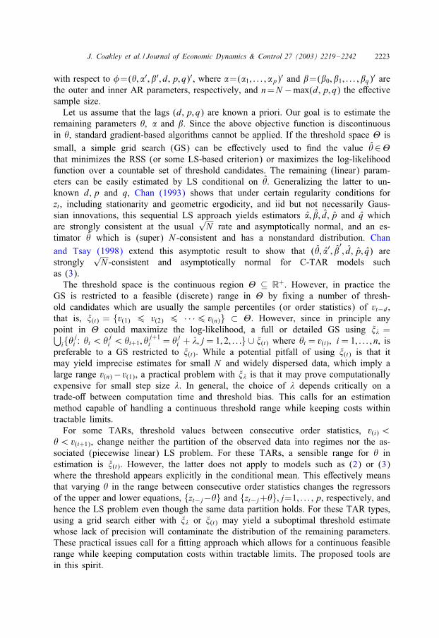
preferable to a GS restricted to �(t). While a potential pitfall of using �(t) is that itmay yield imprecise estimates for small N and widely dispersed data, which imply alarge range v(n)−v(1), a practical problem with �� is that it may prove computationallyexpensive for small step size �. In general, the choice of � depends critically on atrade-oC between computation time and threshold bias. This calls for an estimationmethod capable of handling a continuous threshold range while keeping costs withintractable limits.For some TARs, threshold values between consecutive order statistics, v(i)¡
¡v(i+1), change neither the partition of the observed data into regimes nor the as-sociated (piecewise linear) LS problem. For these TARs, a sensible range for inestimation is �(t). However, the latter does not apply to models such as (2) or (3)where the threshold appears explicitly in the conditional mean. This eCectively meansthat varying in the range between consecutive order statistics changes the regressorsof the upper and lower equations, {zt−j−} and {zt−j+}; j=1; : : : ; p, respectively, andhence the LS problem even though the same data partition holds. For these TAR types,using a grid search either with �� or �(t) may yield a suboptimal threshold estimatewhose lack of precision will contaminate the distribution of the remaining parameters.These practical issues call for a <tting approach which allows for a continuous feasiblerange while keeping computation costs within tractable limits. The proposed tools arein this spirit.
2224 J. Coakley et al. / Journal of Economic Dynamics & Control 27 (2003) 2219–2242
3. An e�cient estimation approach
3.1. Arranged autoregression and threshold intervals
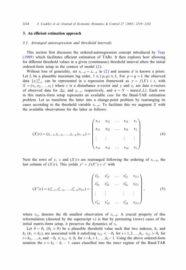
This section <rst discusses the ordered-autoregression concept introduced by Tsay(1989) which facilitates e3cient estimation of TARs. It then explores how allowingfor diCerent threshold values in a given (continuous) threshold interval alters the initialordered-form setup in the context of model (2).Without loss of generality, set vt−d = zt−d in (2) and assume d is known a priori.
Let L be a plausible maximum lag order, 16 (p; q)6L. For p= q= L the observeddata {zt}Nt=1 can be represented in a regression framework as y = f(X ) + , withX = (x1; x2; : : : ; xL) where is a disturbance n-vector and y and xj are data n-vectorsof observed data for Pzt and zt−j, respectively, and n = N − max(d; L). Each rowin this matrix-form setup represents an available case for the Band-TAR estimationproblem. Let us transform the latter into a change-point problem by rearranging itscases according to the threshold variable vt−d. To facilitate this we augment X withthe available observations for the latter as follows:
(X |v) = (zt−1; zt−2; : : : ; zt−L|vt−d) =
x11 x12 : : : x1L v1
x21 x22 : : : x2L v2
......
......
xn1 xn2 : : : xnL vn
: (4)
Next the rows of y; and (X |v) are rearranged following the ordering of vt−d, thelast column of (X |v). This yields yv = f(X v) + v with
(X v|v) = (zvt−1; zvt−2; : : : ; z
vt−L|v(i)) =
xv11 xv12 : : : xv1L v(1)
xv21 xv22 : : : xv2L v(2)
......
......
xvn1 xvn2 : : : xvnL v(n)
; (5)
where v(i) denotes the ith smallest observation of vt−d. A crucial property of thisreformulation (denoted by the superscript v) is that by permuting (rows) cases of theinitial matrix-form setup, it preserves the dynamics of zt .
Let = k (k ¿ 0) be a plausible threshold value such that two indexes, k1 andk2 (k1¡k2), are associated with it satisfying v(i)¡−k for i=1; 2 : : : ; k1; v(i)¿k fori=k2; : : : ; n, and −k6 v(i) 6 k for i=k1+1; : : : ; k2−1. Using the above ordered-formnotation the s = k2 − k1 − 1 cases classi<ed into the inner regime of the Band-TAR
J. Coakley et al. / Journal of Economic Dynamics & Control 27 (2003) 2219–2242 2225
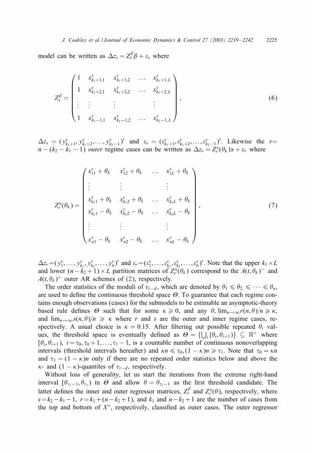
model can be written as Pzs = Z�s � + s where
Z�s =
1 xvk1+1;1 xvk1+1;2 : : : xvk1+1; L
1 xvk1+2;1 xvk1+2;2 : : : xvk1+2; L
......
......
1 xvk2−1;1 xvk2−1;2 : : : xvk2−1; L
; (6)
Pzs = (yvk1+1; yvk1+2; : : : ; y
vk2−1)
′ and s = ( vk1+1; vk1+2; : : : ;
vk2−1)
′. Likewise the r=n− (k2 − k1 − 1) outer regime cases can be written as Pzr = Z�r (k)�+ r where
Z�r (k) =
xv11 + k xv12 + k : : : xv1L + k
......
...
xvk11 + k xvk12 + k : : : xvk1L + k
xvk21 − k xvk22 − k : : : xvk2L − k
......
...
xvn1 − k xvn2 − k : : : xvnL − k
; (7)
Pzr=(yv1; : : : ; yvk1 ; y
vk2 ; : : : ; y
vn)
′ and r=( v1; : : : ; vk1 ;
vk2 ; : : : ;
vn)
′. Note that the upper k1×Land lower (n− k2 +1)×L partition matrices of Z�r (k) correspond to the A(t; k)− andA(t; k)+ outer AR schemes of (2), respectively.The order statistics of the moduli of vt−d, which are denoted by 16 2 6 · · ·6 n,
are used to de<ne the continuous threshold space �. To guarantee that each regime con-tains enough observations (cases) for the submodels to be estimable an asymptotic-theorybased rule de<nes � such that for some '¿ 0, and any ; limn→∞r(n; )=n¿ ',and limn→∞s(n; )=n ¿ ' where r and s are the outer and inner regime cases, re-spectively. A usual choice is ' = 0:15. After <ltering out possible repeated i val-ues, the threshold space is eventually de<ned as � = {⋃i [i; i+1)} ⊆ R+ where[i; i+1); i= )0; )0 +1; : : : ; )1−1, is a countable number of continuous nonoverlappingintervals (threshold intervals hereafter) and 'n6 )0; (1 − ')n¿ )1. Note that )0 = 'nand )1 = (1 − ')n only if there are no repeated order statistics below and above the'- and (1− ')-quantiles of vt−d, respectively.Without loss of generality, let us start the iterations from the extreme right-hand
interval [)1−1; )1 ) in � and allow = )1−1 as the <rst threshold candidate. Thelatter de<nes the inner and outer regressor matrices, Z�s and Z�r (), respectively, wheres=k2−k1−1; r=k1+(n−k2+1), and k1 and n−k2+1 are the number of cases fromthe top and bottom of X v, respectively, classi<ed as outer cases. The outer regressor
2226 J. Coakley et al. / Journal of Economic Dynamics & Control 27 (2003) 2219–2242
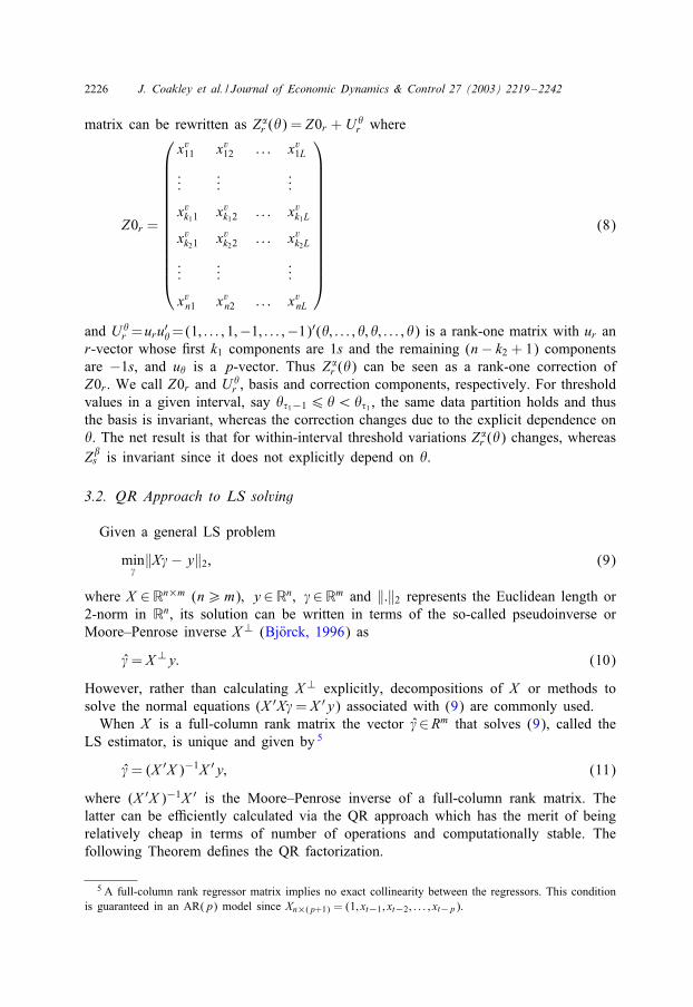
matrix can be rewritten as Z�r () = Z0r + Ur where
Z0r =
xv11 xv12 : : : xv1L...
......
xvk11 xvk12 : : : xvk1L
xvk21 xvk22 : : : xvk2L...
......
xvn1 xvn2 : : : xvnL
(8)
and Ur =uru
′=(1; : : : ; 1;−1; : : : ;−1)′(; : : : ; ; ; : : : ; ) is a rank-one matrix with ur an
r-vector whose <rst k1 components are 1s and the remaining (n− k2 + 1) componentsare −1s, and u is a p-vector. Thus Z�r () can be seen as a rank-one correction ofZ0r . We call Z0r and U
r , basis and correction components, respectively. For thresholdvalues in a given interval, say )1−16 ¡)1 , the same data partition holds and thusthe basis is invariant, whereas the correction changes due to the explicit dependence on. The net result is that for within-interval threshold variations Z�r () changes, whereasZ�s is invariant since it does not explicitly depend on .
3.2. QR Approach to LS solving
Given a general LS problem
min,‖X,− y‖2; (9)
where X ∈Rn×m (n¿m); y∈Rn; ,∈Rm and ‖:‖2 represents the Euclidean length or2-norm in Rn, its solution can be written in terms of the so-called pseudoinverse orMoore–Penrose inverse X⊥ (BjRorck, 1996) as
,= X⊥y: (10)
However, rather than calculating X⊥ explicitly, decompositions of X or methods tosolve the normal equations (X ′X,= X ′y) associated with (9) are commonly used.When X is a full-column rank matrix the vector ,∈Rm that solves (9), called the
LS estimator, is unique and given by 5
,= (X ′X )−1X ′y; (11)
where (X ′X )−1X ′ is the Moore–Penrose inverse of a full-column rank matrix. Thelatter can be e3ciently calculated via the QR approach which has the merit of beingrelatively cheap in terms of number of operations and computationally stable. Thefollowing Theorem de<nes the QR factorization.
5 A full-column rank regressor matrix implies no exact collinearity between the regressors. This conditionis guaranteed in an AR(p) model since Xn×(p+1) = (1; xt−1; xt−2; : : : ; xt−p).
J. Coakley et al. / Journal of Economic Dynamics & Control 27 (2003) 2219–2242 2227
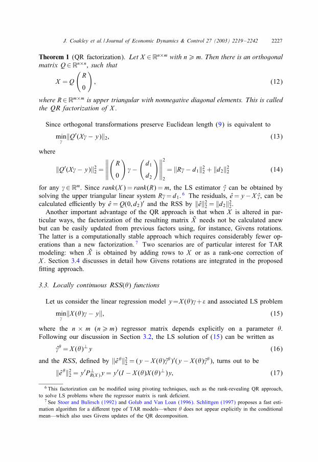
Theorem 1 (QR factorization). Let X ∈Rn×m with n¿m. Then there is an orthogonalmatrix Q∈Rn×n, such that
X = Q
(R
0
); (12)
where R∈Rm×m is upper triangular with nonnegative diagonal elements. This is calledthe QR factorization of X .
Since orthogonal transformations preserve Euclidean length (9) is equivalent to
min,‖Q′(X,− y)‖2; (13)
where
‖Q′(X,− y)‖22 =∥∥∥∥∥(R
0
),−
(d1
d2
)∥∥∥∥∥2
2
= ‖R,− d1‖22 + ‖d2‖22 (14)
for any ,∈Rm. Since rank(X ) = rank(R) =m, the LS estimator , can be obtained bysolving the upper triangular linear system R,=d1. 6 The residuals, e=y−X ,, can becalculated e3ciently by e = Q(0; d2)′ and the RSS by ‖e‖22 = ‖d2‖22.Another important advantage of the QR approach is that when X is altered in par-
ticular ways, the factorization of the resulting matrix X needs not be calculated anewbut can be easily updated from previous factors using, for instance, Givens rotations.The latter is a computationally stable approach which requires considerably fewer op-erations than a new factorization. 7 Two scenarios are of particular interest for TARmodeling: when X is obtained by adding rows to X or as a rank-one correction ofX . Section 3.4 discusses in detail how Givens rotations are integrated in the proposed<tting approach.
3.3. Locally continuous RSS() functions
Let us consider the linear regression model y=X (),+ and associated LS problem
min,‖X (),− y‖; (15)
where the n × m (n¿m) regressor matrix depends explicitly on a parameter .Following our discussion in Section 3.2, the LS solution of (15) can be written as
, = X ()⊥y (16)
and the RSS, de<ned by ‖e ‖22 = (y − X (),)′(y − X (),), turns out to be
‖e ‖22 = y′P⊥R(X )y = y′(I − X ()X ()⊥)y; (17)
6 This factorization can be modi<ed using pivoting techniques, such as the rank-revealing QR approach,to solve LS problems where the regressor matrix is rank de<cient.
7 See Stoer and Bulirsch (1992) and Golub and Van Loan (1996). Schlittgen (1997) proposes a fast esti-mation algorithm for a diCerent type of TAR models—where does not appear explicitly in the conditionalmean—which also uses Givens updates of the QR decomposition.
2228 J. Coakley et al. / Journal of Economic Dynamics & Control 27 (2003) 2219–2242
where P⊥R(X ) is the orthogonal projection of Rn onto the range of X () and I is the
identity matrix.If X () is full-column rank, then the second-moment matrix X ()′X () is
nonsingular and (17) can be computed by
‖e ‖22 = y′(I − X ()(X ()′X ())−1X ()′)y: (18)
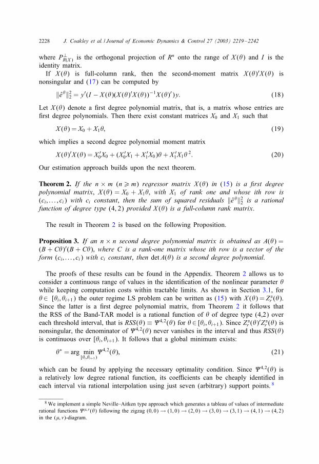
Let X () denote a <rst degree polynomial matrix, that is, a matrix whose entries are<rst degree polynomials. Then there exist constant matrices X0 and X1 such that
X () = X0 + X1; (19)
which implies a second degree polynomial moment matrix
X ()′X () = X ′0X0 + (X ′
0X1 + X ′1X0)+ X ′
1X1 2: (20)
Our estimation approach builds upon the next theorem.
Theorem 2. If the n × m (n¿m) regressor matrix X () in (15) is a -rst degreepolynomial matrix, X () = X0 + X1, with X1 of rank one and whose ith row is(ci; : : : ; ci) with ci constant, then the sum of squared residuals ‖e ‖22 is a rationalfunction of degree type (4, 2) provided X () is a full-column rank matrix.
The result in Theorem 2 is based on the following Proposition.
Proposition 3. If an n × n second degree polynomial matrix is obtained as A() =(B + C)′(B + C), where C is a rank-one matrix whose ith row is a vector of theform (ci; : : : ; ci) with ci constant, then det A() is a second degree polynomial.
The proofs of these results can be found in the Appendix. Theorem 2 allows us toconsider a continuous range of values in the identi<cation of the nonlinear parameter while keeping computation costs within tractable limits. As shown in Section 3.1, for∈ [i; i+1) the outer regime LS problem can be written as (15) with X () = Z�r ().Since the latter is a <rst degree polynomial matrix, from Theorem 2 it follows thatthe RSS of the Band-TAR model is a rational function of of degree type (4,2) overeach threshold interval, that is RSS() ≡ 44;2() for ∈ [i; i+1). Since Z�r ()
′Z�r () isnonsingular, the denominator of 44;2() never vanishes in the interval and thus RSS()is continuous over [i; i+1). It follows that a global minimum exists:
∗ = arg min[i ;i+1)
44;2(); (21)
which can be found by applying the necessary optimality condition. Since 44;2() isa relatively low degree rational function, its coe3cients can be cheaply identi<ed ineach interval via rational interpolation using just seven (arbitrary) support points. 8
8 We implement a simple Neville–Aitken type approach which generates a tableau of values of intermediaterational functions 45;6() following the zigzag (0; 0) → (1; 0) → (2; 0) → (3; 0) → (3; 1) → (4; 1) → (4; 2)in the (5; 6)-diagram.
J. Coakley et al. / Journal of Economic Dynamics & Control 27 (2003) 2219–2242 2229
3.4. QR updating: Givens transformations
This section discusses, <rst, how Givens rotations can be used to iterate e3cientlywithin and across thershold intervals and, second, how the lags p; q and d can beidenti<ed.For the outer regime, the algorithm starts by considering the submodel for p = L.
The outer-regime LS problem for any ∈ [i; i+1) can be written as
min�‖Z�r ()�−Pzr‖2; (22)
where, as shown in Section 3.1, its r × L regressor matrix has two components, thebasis Z0r and the correction U
r ; Z�r ()=Z0r +U
r . Since within-interval variations of
aCect only Ur , it follows that the LS problems associated with diCerent candidates
in [i; i+1) can be solved readily by simply updating the QR factors of Z�r () forthe diCerent U
r . Moreover, since Z�r () is just a rank-one correction of Z0r , thesewithin-interval updates can be cheaply obtained via Givens rotations.Now let us consider across-interval variations of , that is, the algorithm moves to
the next (say, contiguous to the left) threshold interval, [i−1; i) ⊂ �. In contrast to thewithin-interval variations, not only does the correction U
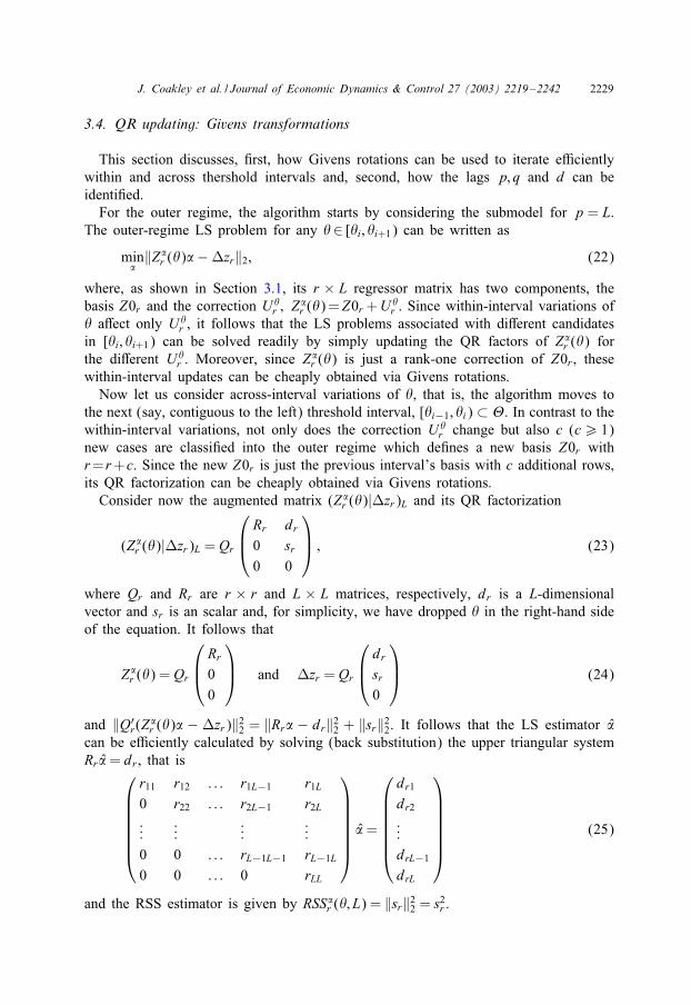
r change but also c (c¿ 1)new cases are classi<ed into the outer regime which de<nes a new basis Z0r withr=r+c. Since the new Z0r is just the previous interval’s basis with c additional rows,its QR factorization can be cheaply obtained via Givens rotations.Consider now the augmented matrix (Z�r ()|Pzr)L and its QR factorization
(Z�r ()|Pzr)L = Qr
Rr dr
0 sr0 0
; (23)
where Qr and Rr are r × r and L × L matrices, respectively, dr is a L-dimensionalvector and sr is an scalar and, for simplicity, we have dropped in the right-hand sideof the equation. It follows that
Z�r () = Qr
Rr
00
and Pzr = Qr
drsr0
(24)
and ‖Q′r(Z
�r ()� − Pzr)‖22 = ‖Rr� − dr‖22 + ‖sr‖22. It follows that the LS estimator �
can be e3ciently calculated by solving (back substitution) the upper triangular systemRr�= dr , that is
r11 r12 : : : r1L−1 r1L0 r22 : : : r2L−1 r2L...
......
...0 0 : : : rL−1L−1 rL−1L
0 0 : : : 0 rLL
�=
dr1dr2...drL−1
drL
(25)
and the RSS estimator is given by RSS�r (; L) = ‖sr‖22 = s2r .
2230 J. Coakley et al. / Journal of Economic Dynamics & Control 27 (2003) 2219–2242
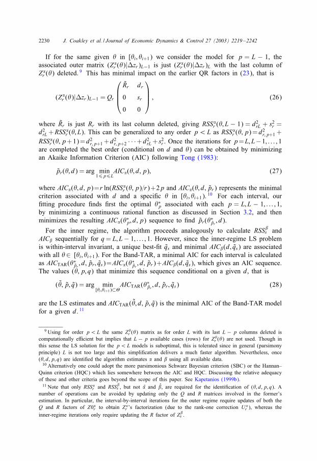
If for the same given in [i; i+1) we consider the model for p = L − 1, theassociated outer matrix (Z�r ()|Pzr)L−1 is just (Z�r ()|Pzr)L with the last column ofZ�r () deleted. 9 This has minimal impact on the earlier QR factors in (23), that is
(Z�r ()|Pzr)L−1 = Qr
Rr dr
0 sr
0 0
; (26)
where Rr is just Rr with its last column deleted, giving RSS�r (; L − 1) = d2rL + s2r =d2rL+RSS
�r (; L). This can be generalized to any order p¡L as RSS�r (; p)=d
2r;p+1 +
RSS�r (; p+1)=d2r;p+1+d2r;p+2 · · ·+d2rL+ s2r . Once the iterations for p=L; L−1; : : : ; 1
are completed the best order (conditional on d and ) can be obtained by minimizingan Akaike Information Criterion (AIC) following Tong (1983):
pr(; d) = arg min16p6L
AIC�(; d; p); (27)
where AIC�(; d; p)=r ln(RSS�r (; p)=r)+2p and AIC�(; d; pr) represents the minimalcriterion associated with d and a speci<c in [i; i+1). 10 For each interval, our<tting procedure <nds <rst the optimal ∗p associated with each p = L; L − 1; : : : ; 1,by minimizing a continuous rational function as discussed in Section 3.2, and thenminimizes the resulting AIC�(∗p; d; p) sequence to <nd pr(∗pr ; d).
For the inner regime, the algorithm proceeds analogously to calculate RSS�s andAIC� sequentially for q= L; L− 1; : : : ; 1. However, since the inner-regime LS problemis within-interval invariant, a unique best-<t qs and minimal AIC�(d; qs) are associatedwith all ∈ [i; i+1). For the Band-TAR, a minimal AIC for each interval is calculatedas AICTAR(∗pr ; d; pr ; qs)=AIC�(
∗pr ; d; pr)+AIC�(d; qs), which gives an AIC sequence.
The values (; p; q) that minimize this sequence conditional on a given d, that is
(; p; q) = arg min[i ;i+1)⊂�
AICTAR(∗pr ; d; pr ; qs) (28)
are the LS estimates and AICTAR(; d; p; q) is the minimal AIC of the Band-TAR modelfor a given d. 11
9 Using for order p¡L the same Zr () matrix as for order L with its last L − p columns deleted iscomputationally e3cient but implies that L − p available cases (rows) for Zr () are not used. Though inthis sense the LS solution for the p¡L models is suboptimal, this is tolerated since in general (parsimonyprinciple) L is not too large and this simpli<cation delivers a much faster algorithm. Nevertheless, once(; d; p; q) are identi<ed the algorithm estimates � and � using all available data.10 Alternatively one could adopt the more parsimonious Schwarz Bayesian criterion (SBC) or the Hannan–
Quinn criterion (HQC) which lies somewhere between the AIC and HQC. Discussing the relative adequacyof these and other criteria goes beyond the scope of this paper. See Kapetanios (1999b).11 Note that only RSS�r and RSS�s , but not � and �, are required for the identi<cation of (; d; p; q). A
number of operations can be avoided by updating only the Q and R matrices involved in the former’sestimation. In particular, the interval-by-interval iterations for the outer regime require updates of both theQ and R factors of Z0�r to obtain Z�r ’s factorization (due to the rank-one correction U�
r ), whereas theinner-regime iterations only require updating the R factor of Z�s .
J. Coakley et al. / Journal of Economic Dynamics & Control 27 (2003) 2219–2242 2231
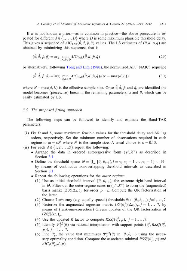
If d is not known a priori—as is common in practice—the above procedure is re-peated for diCerent d∈{1; : : : ; D} where D is some maximum plausible threshold delay.This gives a sequence of AICTAR(; d; p; q) values. The LS estimates of (; d; p; q) areobtained by minimizing this sequence, that is
(; d; p; q) = arg min16d6D
AICTAR(; d; p; q) (29)
or alternatively, following Tong and Lim (1980), the normalized AIC (NAIC) sequence
(; d; p; q) = arg min16d6D
AICTAR(; d; p; q)=(N −max(d; L)) (30)
where N −max(d; L) is the eCective sample size. Once ; d; p and q, are identi<ed themodel becomes (piecewise) linear in the remaining parameters, � and �, which can beeasily estimated by LS.
3.5. The proposed -tting approach
The following steps can be followed to identify and estimate the Band-TARparameters:
(i) Fix D and L, some maximum feasible values for the threshold delay and AR lagorders, respectively. Set the minimum number of observations required in eachregime to m= 'N where N is the sample size. A usual choice is ' = 0:15.
(ii) For each d∈{1; 2; : : : ; D} repeat the following:• Arrange the data in ordered autoregressive form (yv; X v) as described in
Section 3.1.• De<ne the threshold space � = {⋃i [i; i+1); i = )0; )0 + 1; : : : ; )1 − 1} ⊂ R+
by means of continuous nonoverlapping thershold intervals as described inSection 3.1.
• Repeat the following operations for the outer regime:(1) Use as initial threshold interval [i; i+1), the extreme right-hand interval
in �. Filter out the outer-regime cases in (yv; X v) to form the (augmented)basis matrix (Z0�r |Pzr)p for order p= L. Compute the QR factorization ofthe latter.
(2) Choose 7 arbitrary (e.g. equally spaced) thresholds ji ∈ [i; i+1); j=1; : : : ; 7.(3) Factorize the augmented regressor matrix (Z�r (
ji)|Pzr)p; j = 1; : : : ; 7, by
means of (rank-one-correction) Givens updates of the QR factorization of(Z0�r |Pzr)p.
(4) Use the updated R factor to compute RSS�r (ji ; p); j = 1; : : : ; 7.
(5) Identify 44;2p () via rational interpolation with support points (ji ; RSS
�r (
ji ;
p)); j = 1; : : : 7.(6) Find ∗p, the value that minimizes 44;2
p () in [i; i+1) using the neces-sary optimality condition. Compute the associated minimal RSS�r (
∗p; p) and
AIC�(∗p; d; p).
2232 J. Coakley et al. / Journal of Economic Dynamics & Control 27 (2003) 2219–2242
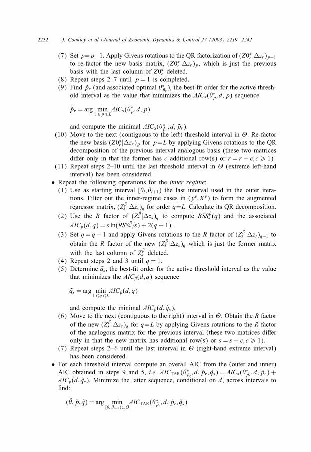
(7) Set p=p−1. Apply Givens rotations to the QR factorization of (Z0�r |Pzr)p+1
to re-factor the new basis matrix, (Z0�r |Pzr)p, which is just the previousbasis with the last column of Z0�r deleted.
(8) Repeat steps 2–7 until p= 1 is completed.(9) Find pr (and associated optimal ∗pr ), the best-<t order for the active thresh-
old interval as the value that minimizes the AIC�(∗p; d; p) sequence
pr = arg min16p6L
AIC�(∗p; d; p)
and compute the minimal AIC�(∗pr ; d; pr).(10) Move to the next (contiguous to the left) threshold interval in �. Re-factor
the new basis (Z0�r |Pzr)p for p=L by applying Givens rotations to the QRdecomposition of the previous interval analogous basis (these two matricesdiCer only in that the former has c additional row(s) or r = r + c; c¿ 1).
(11) Repeat steps 2–10 until the last threshold interval in � (extreme left-handinterval) has been considered.
• Repeat the following operations for the inner regime:(1) Use as starting interval [i; i+1) the last interval used in the outer itera-
tions. Filter out the inner-regime cases in (yv; X v) to form the augmentedregressor matrix, (Z�s |Pzs)q for order q=L. Calculate its QR decomposition.
(2) Use the R factor of (Z�s |Pzs)q to compute RSS�s (q) and the associatedAIC�(d; q) = s ln(RSS�s =s) + 2(q+ 1).
(3) Set q= q− 1 and apply Givens rotations to the R factor of (Z�s |Pzs)q+1 toobtain the R factor of the new (Z�s |Pzs)q which is just the former matrixwith the last column of Z�s deleted.
(4) Repeat steps 2 and 3 until q= 1.(5) Determine qs, the best-<t order for the active threshold interval as the value
that minimizes the AIC�(d; q) sequence
qs = arg min16q6L
AIC�(d; q)
and compute the minimal AIC�(d; qs).(6) Move to the next (contiguous to the right) interval in �. Obtain the R factor
of the new (Z�s |Pzs)q for q=L by applying Givens rotations to the R factorof the analogous matrix for the previous interval (these two matrices diCeronly in that the new matrix has additional row(s) or s= s+ c; c¿ 1).
(7) Repeat steps 2–6 until the last interval in � (right-hand extreme interval)has been considered.
• For each threshold interval compute an overall AIC from the (outer and inner)AIC obtained in steps 9 and 5, i.e. AICTAR(∗pr ; d; pr ; qs) = AIC�(∗pr ; d; pr) +AIC�(d; qs). Minimize the latter sequence, conditional on d, across intervals to<nd:
(; p; q) = arg min[i ;i+1)⊂�
AICTAR(∗pr ; d; pr ; qs)
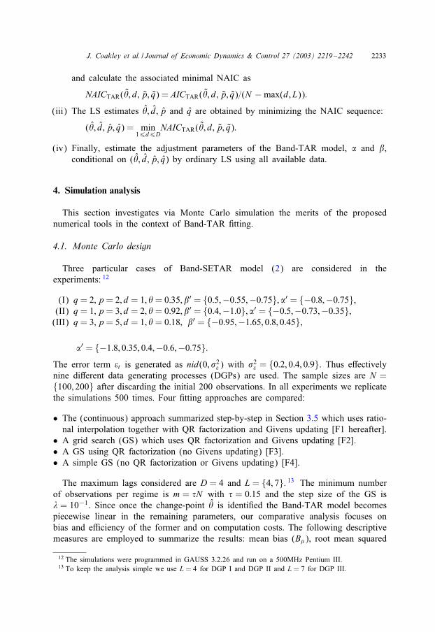
J. Coakley et al. / Journal of Economic Dynamics & Control 27 (2003) 2219–2242 2233
and calculate the associated minimal NAIC as
NAICTAR(; d; p; q) = AICTAR(; d; p; q)=(N −max(d; L)):
(iii) The LS estimates ; d; p and q are obtained by minimizing the NAIC sequence:
(; d; p; q) = min16d6D
NAICTAR(; d; p; q):
(iv) Finally, estimate the adjustment parameters of the Band-TAR model, � and �,conditional on (; d; p; q) by ordinary LS using all available data.
4. Simulation analysis
This section investigates via Monte Carlo simulation the merits of the proposednumerical tools in the context of Band-TAR <tting.
4.1. Monte Carlo design
Three particular cases of Band-SETAR model (2) are considered in theexperiments: 12
(I) q= 2; p= 2; d= 1; = 0:35; �′ = {0:5;−0:55;−0:75}; �′ = {−0:8;−0:75},(II) q= 1; p= 3; d= 2; = 0:92; �′ = {0:4;−1:0}; �′ = {−0:5;−0:73;−0:35},(III) q= 3; p= 5; d= 1; = 0:18; �′ = {−0:95;−1:65; 0:8; 0:45},
�′ = {−1:8; 0:35; 0:4;−0:6;−0:75}:The error term t is generated as nid(0; �2 ) with �2 = {0:2; 0:4; 0:9}. Thus eCectivelynine diCerent data generating processes (DGPs) are used. The sample sizes are N ={100; 200} after discarding the initial 200 observations. In all experiments we replicatethe simulations 500 times. Four <tting approaches are compared:
• The (continuous) approach summarized step-by-step in Section 3.5 which uses ratio-nal interpolation together with QR factorization and Givens updating [F1 hereafter].
• A grid search (GS) which uses QR factorization and Givens updating [F2].• A GS using QR factorization (no Givens updating) [F3].• A simple GS (no QR factorization or Givens updating) [F4].
The maximum lags considered are D = 4 and L = {4; 7}. 13 The minimum numberof observations per regime is m = )N with ) = 0:15 and the step size of the GS is� = 10−1. Since once the change-point is identi<ed the Band-TAR model becomespiecewise linear in the remaining parameters, our comparative analysis focuses onbias and e3ciency of the former and on computation costs. The following descriptivemeasures are employed to summarize the results: mean bias (B5), root mean squared
12 The simulations were programmed in GAUSS 3.2.26 and run on a 500MHz Pentium III.13 To keep the analysis simple we use L = 4 for DGP I and DGP II and L = 7 for DGP III.
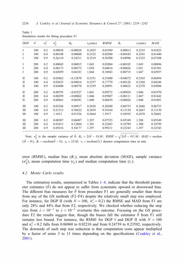
2234 J. Coakley et al. / Journal of Economic Dynamics & Control 27 (2003) 2219–2242
Table 1Simulation results for <tting procedure F1
DGP N �2 �2
B5 t5(min) RMSE B) t)(min) MAD
I 100 0.2 0.00038 −0:00028 0.2425 0.01949 0.00013 0.2335 0.01023I 100 0.4 0.00108 0.00060 0.2332 0.02940 −0:00105 0.2341 0.01440I 100 0.9 0.26110 0.24211 0.2319 0.56500 0.04996 0.2325 0.07308
I 200 0.2 0.00045 0.00015 1.043 0.02084 −0:00102 1.043 0.00896I 200 0.4 0.00173 0.00372 1.058 0.04014 −0:00026 1.051 0.01501I 200 0.9 0.02059 0.04181 1.044 0.10943 0.00715 1.047 0.02957
II 100 0.2 0.03862 −0:12870 0.2351 0.23480 −0:04672 0.2365 0.06494II 100 0.4 0.03635 −0:04014 0.2357 0.17770 −0:00126 0.2368 0.04246II 100 0.9 0.04400 0.00578 0.2359 0.20891 0.00623 0.2370 0.05006
II 200 0.2 0.00793 −0:03527 1.041 0.09572 −0:00924 1.046 0.01970II 200 0.4 0.00299 −0:00062 1.046 0.05807 −0:00111 1.047 0.01642II 200 0.9 0.00463 0.00281 1.040 0.06839 −0:00026 1.040 0.01881
III 100 0.2 0.03246 0.09917 0.2658 0.20280 0.06753 0.2666 0.06753III 100 0.4 0.21313 0.30622 0.2659 0.54164 0.13130 0.2667 0.13130III 100 0.9 1.1013 0.91536 0.2664 1.3917 0.28592 0.2670 0.28601
III 200 0.2 0.00207 0.06007 1.287 0.07535 0.05349 1.288 0.05349III 200 0.4 0.03413 0.12804 1.301 0.22463 0.10799 1.300 0.10799III 200 0.9 0.69216 0.54177 1.297 0.99211 0.22343 1.297 0.22343
Note: �2is the sample variance of ; B5 = 8( − )=M ; RMSE =
√8(− )2=M ; MAD = median
(|− |); B) = median(− ); t5 = 8t=M ; t) = median(t); t denotes computation time in min.
error (RMSE), median bias (B)), mean absolute deviation (MAD), sample variance(�2), mean computation time (t5) and median computation time (t)).
4.2. Monte Carlo results
The estimation results, summarized in Tables 1–4, indicate that the threshold param-eter estimates () do not appear to suCer from systematic upward or downward bias.The diCerent bias measures for from procedure F1 are generally smaller than thosefrom any of the GS methods (F2–F4) despite the relatively small step size employed.For instance, for DGP II (with N = 100; �2 = 0:2) the RMSE and MAD from F1 areonly 28% and 44% that from F2, respectively. We checked whether reducing the stepsize from � = 10−1 to � = 10−3 overturns this outcome. Focusing on the GS proce-dure F2 the results suggest that, though the biases fall the estimator from F1 stillremains less biased. For instance, the RMSE for DGP I and DGP II with N = 100and �2 =0:2 falls from 0.06960 to 0.02210 and from 0.24739 to 0.23592, respectively.The downside of such step size reduction is that computation costs appear multipliedby a factor of some 3 to 13 times depending on the speci<cations (Coakley et al.,2001).
J. Coakley et al. / Journal of Economic Dynamics & Control 27 (2003) 2219–2242 2235
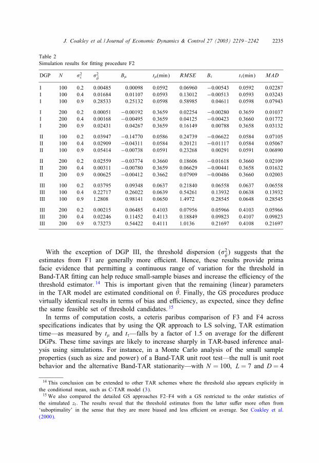
Table 2Simulation results for <tting procedure F2
DGP N �2 �2
B5 t5(min) RMSE B) t)(min) MAD
I 100 0.2 0.00485 0.00098 0.0592 0.06960 −0:00543 0.0592 0.02287I 100 0.4 0.01684 0.01107 0.0593 0.13012 −0:00513 0.0593 0.03243I 100 0.9 0.28533 0.25132 0.0598 0.58985 0.04611 0.0598 0.07943
I 200 0.2 0.00051 −0:00192 0.3659 0.02254 −0:00280 0.3659 0.01037I 200 0.4 0.00168 −0:00495 0.3659 0.04125 −0:00423 0.3660 0.01772I 200 0.9 0.02431 0.04267 0.3659 0.16149 0.00788 0.3658 0.03132
II 100 0.2 0.03947 −0:14770 0.0586 0.24739 −0:06622 0.0584 0.07105II 100 0.4 0.02909 −0:04311 0.0584 0.20121 −0:01117 0.0584 0.05067II 100 0.9 0.05414 −0:00738 0.0591 0.23268 0.00291 0.0591 0.06890
II 200 0.2 0.02559 −0:03774 0.3660 0.18606 −0:01618 0.3660 0.02109II 200 0.4 0.00311 −0:00780 0.3659 0.06629 −0:00441 0.3658 0.01632II 200 0.9 0.00625 −0:00412 0.3662 0.07909 −0:00486 0.3660 0.02003
III 100 0.2 0.03795 0.09348 0.0637 0.21840 0.06558 0.0637 0.06558III 100 0.4 0.22717 0.26022 0.0639 0.54261 0.13932 0.0638 0.13932III 100 0.9 1.2808 0.98141 0.0650 1.4972 0.28545 0.0648 0.28545
III 200 0.2 0.00215 0.06485 0.4103 0.07956 0.05966 0.4103 0.05966III 200 0.4 0.02246 0.11452 0.4113 0.18849 0.09823 0.4107 0.09823III 200 0.9 0.73273 0.54422 0.4111 1.0136 0.21697 0.4108 0.21697
With the exception of DGP III, the threshold dispersion (�2) suggests that the
estimates from F1 are generally more e3cient. Hence, these results provide primafacie evidence that permitting a continuous range of variation for the threshold inBand-TAR <tting can help reduce small-sample biases and increase the e3ciency of thethreshold estimator. 14 This is important given that the remaining (linear) parametersin the TAR model are estimated conditional on . Finally, the GS procedures producevirtually identical results in terms of bias and e3ciency, as expected, since they de<nethe same feasible set of threshold candidates. 15
In terms of computation costs, a ceteris paribus comparison of F3 and F4 acrossspeci<cations indicates that by using the QR approach to LS solving, TAR estimationtime—as measured by t5 and t)—falls by a factor of 1.5 on average for the diCerentDGPs. These time savings are likely to increase sharply in TAR-based inference anal-ysis using simulations. For instance, in a Monte Carlo analysis of the small sampleproperties (such as size and power) of a Band-TAR unit root test—the null is unit rootbehavior and the alternative Band-TAR stationarity—with N = 100; L = 7 and D = 4
14 This conclusion can be extended to other TAR schemes where the threshold also appears explicitly inthe conditional mean, such as C-TAR model (3).15 We also compared the detailed GS approaches F2–F4 with a GS restricted to the order statistics of
the simulated zt . The results reveal that the threshold estimates from the latter suCer more often from‘suboptimality’ in the sense that they are more biased and less e3cient on average. See Coakley et al.(2000).
2236 J. Coakley et al. / Journal of Economic Dynamics & Control 27 (2003) 2219–2242
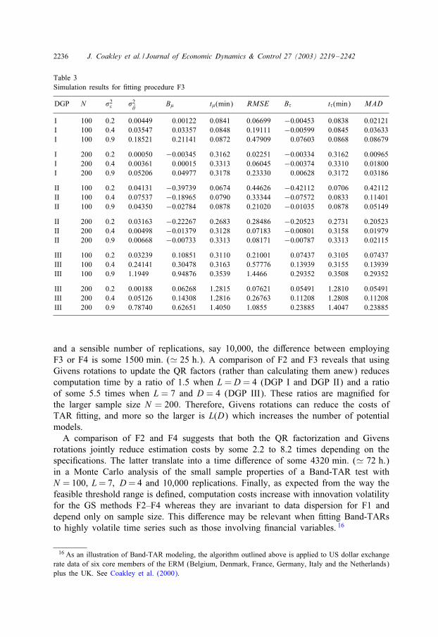
Table 3Simulation results for <tting procedure F3
DGP N �2 �2
B5 t5(min) RMSE B) t)(min) MAD
I 100 0.2 0.00449 0.00122 0.0841 0.06699 −0:00453 0.0838 0.02121I 100 0.4 0.03547 0.03357 0.0848 0.19111 −0:00599 0.0845 0.03633I 100 0.9 0.18521 0.21141 0.0872 0.47909 0.07603 0.0868 0.08679
I 200 0.2 0.00050 −0:00345 0.3162 0.02251 −0:00334 0.3162 0.00965I 200 0.4 0.00361 0.00015 0.3313 0.06045 −0:00374 0.3310 0.01800I 200 0.9 0.05206 0.04977 0.3178 0.23330 0.00628 0.3172 0.03186
II 100 0.2 0.04131 −0:39739 0.0674 0.44626 −0:42112 0.0706 0.42112II 100 0.4 0.07537 −0:18965 0.0790 0.33344 −0:07572 0.0833 0.11401II 100 0.9 0.04350 −0:02784 0.0878 0.21020 −0:01035 0.0878 0.05149
II 200 0.2 0.03163 −0:22267 0.2683 0.28486 −0:20523 0.2731 0.20523II 200 0.4 0.00498 −0:01379 0.3128 0.07183 −0:00801 0.3158 0.01979II 200 0.9 0.00668 −0:00733 0.3313 0.08171 −0:00787 0.3313 0.02115
III 100 0.2 0.03239 0.10851 0.3110 0.21001 0.07437 0.3105 0.07437III 100 0.4 0.24141 0.30478 0.3163 0.57776 0.13939 0.3155 0.13939III 100 0.9 1.1949 0.94876 0.3539 1.4466 0.29352 0.3508 0.29352
III 200 0.2 0.00188 0.06268 1.2815 0.07621 0.05491 1.2810 0.05491III 200 0.4 0.05126 0.14308 1.2816 0.26763 0.11208 1.2808 0.11208III 200 0.9 0.78740 0.62651 1.4050 1.0855 0.23885 1.4047 0.23885
and a sensible number of replications, say 10,000, the diCerence between employingF3 or F4 is some 1500 min: (� 25 h:). A comparison of F2 and F3 reveals that usingGivens rotations to update the QR factors (rather than calculating them anew) reducescomputation time by a ratio of 1.5 when L= D = 4 (DGP I and DGP II) and a ratioof some 5.5 times when L = 7 and D = 4 (DGP III). These ratios are magni<ed forthe larger sample size N = 200. Therefore, Givens rotations can reduce the costs ofTAR <tting, and more so the larger is L(D) which increases the number of potentialmodels.A comparison of F2 and F4 suggests that both the QR factorization and Givens
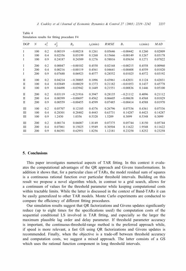
rotations jointly reduce estimation costs by some 2.2 to 8.2 times depending on thespeci<cations. The latter translate into a time diCerence of some 4320 min: (� 72 h:)in a Monte Carlo analysis of the small sample properties of a Band-TAR test withN = 100, L= 7; D= 4 and 10,000 replications. Finally, as expected from the way thefeasible threshold range is de<ned, computation costs increase with innovation volatilityfor the GS methods F2–F4 whereas they are invariant to data dispersion for F1 anddepend only on sample size. This diCerence may be relevant when <tting Band-TARsto highly volatile time series such as those involving <nancial variables. 16
16 As an illustration of Band-TAR modeling, the algorithm outlined above is applied to US dollar exchangerate data of six core members of the ERM (Belgium, Denmark, France, Germany, Italy and the Netherlands)plus the UK. See Coakley et al. (2000).
J. Coakley et al. / Journal of Economic Dynamics & Control 27 (2003) 2219–2242 2237
Table 4Simulation results for <tting procedure F4
DGP N �2 �2
B5 t5(min) RMSE B) t)(min) MAD
I 100 0.2 0.00319 −0:00218 0.1261 0.05646 −0:00442 0.1260 0.02009I 100 0.4 0.02356 0.03199 0.1268 0.15666 −0:00149 0.1267 0.03178I 100 0.9 0.24187 0.24309 0.1276 0.58816 0.05634 0.1271 0.07822
I 200 0.2 0.00047 −0:00102 0.4558 0.02168 −0:00215 0.4558 0.00960I 200 0.4 0.00216 −0:00119 0.4561 0.04641 −0:00408 0.4559 0.01820I 200 0.9 0.07688 0.06923 0.4577 0.28552 0.01025 0.4572 0.03192
II 100 0.2 0.04214 −0:38885 0.1096 0.43961 −0:42031 0.1124 0.42031II 100 0.4 0.03849 −0:08029 0.1373 0.21182 −0:01053 0.1437 0.45778II 100 0.9 0.04498 −0:03942 0.1449 0.21551 −0:00836 0.1446 0.05100
II 200 0.2 0.03119 −0:21916 0.3947 0.28135 −0:21112 0.4096 0.21112II 200 0.4 0.00399 −0:00697 0.4562 0.06605 −0:00638 0.4568 0.01829II 200 0.9 0.00559 −0:00455 0.4599 0.07485 −0:00414 0.4588 0.01970
III 100 0.2 0.05707 0.12185 0.4376 0.26796 0.07536 0.4361 0.07536III 100 0.4 0.28301 0.28402 0.4443 0.63731 0.14287 0.4423 0.14287III 100 0.9 1.2430 1.0356 0.5328 1.5209 0.3099 0.5348 0.3099
III 200 0.2 0.00174 0.06087 1.8149 0.07375 0.05744 1.8150 0.05744III 200 0.4 0.07061 0.15025 1.9549 0.30504 0.11622 1.9548 0.11622III 200 0.9 0.86391 0.62951 1.8256 1.12181 0.23258 1.8252 0.23258
5. Conclusions
This paper investigates numerical aspects of TAR <tting. In this context it evalu-ates the computational advantages of the QR approach and Givens transformations. Inaddition it shows that, for a particular class of TARs, the model residual sum of squaresis a continuous rational function over particular threshold intervals. Building on thisresult we propose a novel algorithm which, in contrast to a grid search, allows fora continuum of values for the threshold parameter while keeping computational costswithin tractable limits. While the latter is discussed in the context of Band-TARs it canbe easily generalized to other TAR models. Monte Carlo experiments are conducted tocompare the e3ciency of diCerent <tting procedures.Our simulation results suggest that QR factorizations and Givens updates signi<cantly
reduce (up to eight times for the speci<cations used) the computation costs of thesequential conditional LS involved in TAR <tting, and especially so the larger themaximum plausible lag order and delay parameter. If threshold parameter accuracyis important, the continuous-threshold-range method is the preferred approach while,if speed is more relevant, a fast GS using QR factorizations and Givens updates isrecommended. Finally, when the objective is a trade-oC between threshold accuracyand computation costs, we suggest a mixed approach. The latter consists of a GSwhich uses the rational function component in long threshold intervals.
2238 J. Coakley et al. / Journal of Economic Dynamics & Control 27 (2003) 2219–2242
Issues for future research include improving the rational interpolation algorithm interms of computation time and stability and investigating further the properties of theresidual sum of squares rational functions.
Acknowledgements
We thank Michel Juillard, Miguel Angel Mart,-n, an anonymous referee and partic-ipants at the Society for Computational Economics 6th CEF International Conference,Universitat Pompeu Fabra, Barcelona, July 2000, for helpful comments.
Appendix.
This appendix includes the proof of the main results in Section 3.3. It starts byproving the following more general result.
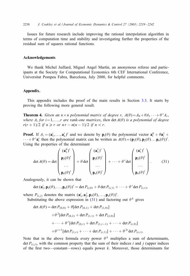
Theorem 4. Given an n×n polynomial matrix of degree r; A()=A0+A1 · · ·+ rAr ,where Ai for i=1; : : : ; r are rank-one matrices, then det A() is a polynomial of degreer(r + 1)=2 if n¿ r or n r − n(n− 1)=2 if n¡r.
Proof. If Ai = (ai1; : : : ; ain)
′ and we denote by pi() the polynomial vector a0i + a1i +· · ·+ rari then the polynomial matrix can be written as A()=(p1(); p2() : : : pn())′.Using the properties of the determinant
det A() = det
(a01)′
p2()′
: : :
pn()′
+ det
(a11)′
p2()′
: : :
pn()′
+ · · ·+ rdet
(ar1)′
p2()′
: : :
pn()′
: (31)
Analogously, it can be shown that
det (ai1; p2(); : : : ; pn())′ = det P(i;0) + det P(i;1) + · · ·+ rdet P(i; r);
where P(i; j) denotes the matrix (ai1; aj2 ; p3(); : : : ; pn())
′.Substituting the above expression in (31) and factoring out k gives
det A() = det P(0;0) + [det P(0;1) + det P(1;0)]
+ 2[det P(0;2) + det P(1;1) + det P(2;0)]
+ · · ·+ r[det P(0; r) + det P(1; r−1) + · · ·+ det P(r;0)]
+ r+1[det P(1; r) + · · ·+ det P(r;1)] + · · ·+ 2rdet P(r; r):
Note that in the above formula every power k multiplies a sum of determinants,det P(i; j), with the common property that the sum of their indices i and j (upper indicesof the <rst two—constant—rows) equals power k. Moreover, those determinants for
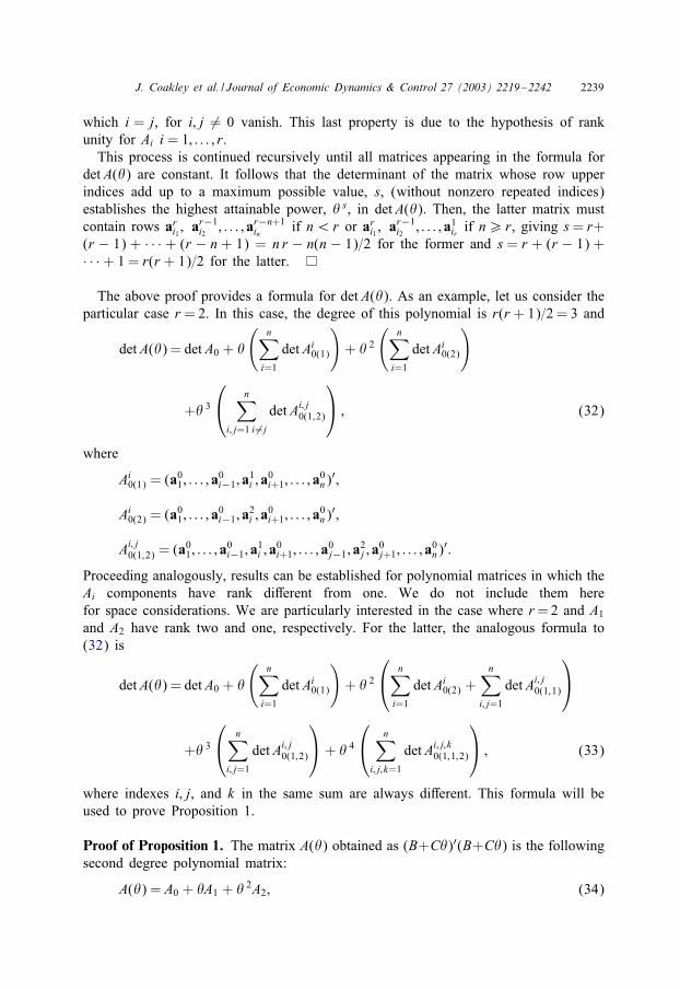
J. Coakley et al. / Journal of Economic Dynamics & Control 27 (2003) 2219–2242 2239
which i = j, for i; j �= 0 vanish. This last property is due to the hypothesis of rankunity for Ai i = 1; : : : ; r.This process is continued recursively until all matrices appearing in the formula for
det A() are constant. It follows that the determinant of the matrix whose row upperindices add up to a maximum possible value, s, (without nonzero repeated indices)establishes the highest attainable power, s, in det A(). Then, the latter matrix mustcontain rows ari1 ; a
r−1i2 ; : : : ; ar−n+1
in if n¡r or ari1 ; ar−1i2 ; : : : ; a1ir if n¿ r, giving s= r+
(r − 1) + · · · + (r − n + 1) = n r − n(n − 1)=2 for the former and s = r + (r − 1) +· · ·+ 1 = r(r + 1)=2 for the latter.
The above proof provides a formula for det A(). As an example, let us consider theparticular case r = 2. In this case, the degree of this polynomial is r(r + 1)=2 = 3 and
det A() = det A0 +
(n∑i=1
det Ai0(1)
)+ 2
(n∑i=1
det Ai0(2)
)
+ 3
n∑i; j=1 i =j
det Ai;j0(1;2)
; (32)
where
Ai0(1) = (a01; : : : ; a0i−1; a
1i ; a
0i+1; : : : ; a
0n)
′;
Ai0(2) = (a01; : : : ; a0i−1; a
2i ; a
0i+1; : : : ; a
0n)
′;
Ai; j0(1;2) = (a01; : : : ; a0i−1; a
1i ; a
0i+1; : : : ; a
0j−1; a
2j ; a
0j+1; : : : ; a
0n)
′:
Proceeding analogously, results can be established for polynomial matrices in which theAi components have rank diCerent from one. We do not include them herefor space considerations. We are particularly interested in the case where r=2 and A1
and A2 have rank two and one, respectively. For the latter, the analogous formula to(32) is
det A() = det A0 +
(n∑i=1
det Ai0(1)
)+ 2
n∑
i=1
det Ai0(2) +n∑
i; j=1
det Ai;j0(1;1)
+ 3
n∑i; j=1
det Ai;j0(1;2)
+ 4
n∑i; j; k=1
det Ai;j; k0(1;1;2)
; (33)
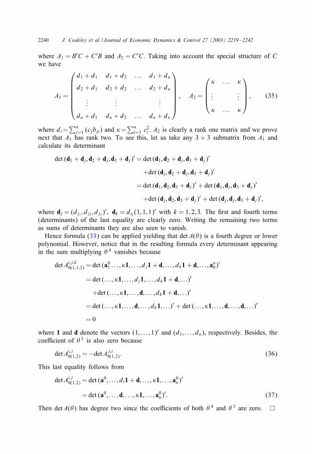
where indexes i; j, and k in the same sum are always diCerent. This formula will beused to prove Proposition 1.
Proof of Proposition 1. The matrix A() obtained as (B+C)′(B+C) is the followingsecond degree polynomial matrix:
A() = A0 + A1 + 2A2; (34)
2240 J. Coakley et al. / Journal of Economic Dynamics & Control 27 (2003) 2219–2242
where A1 = B′C + C′B and A2 = C′C. Taking into account the special structure of Cwe have
A1 =
d1 + d1 d1 + d2 : : : d1 + dn
d2 + d1 d2 + d2 : : : d2 + dn
......
...
dn + d1 dn + d2 : : : dn + dn
; A2 =
' : : : '
......
' : : : '
; (35)
where di=∑n
j=1 (cjbji) and '=∑n
i=1 c2i : A2 is clearly a rank one matrix and we prove
next that A1 has rank two. To see this, let us take any 3 × 3 submatrix from A1 andcalculate its determinant
det (d1 + dj; d2 + dj; d3 + dj)′ = det (d1; d2 + dj; d3 + dj)′
+det (dj; d2 + dj; d3 + dj)′
= det (d1; d2; d3 + dj)′ + det (d1; dj; d3 + dj)′
+det (dj; d2; d3 + dj)′ + det (dj; dj; d3 + dj)′;
where dj = (dj1 ; dj2 ; dj3 )′; dk = dik (1; 1; 1)
′ with k = 1; 2; 3. The <rst and fourth terms(determinants) of the last equality are clearly zero. Writing the remaining two termsas sums of determinants they are also seen to vanish.Hence formula (33) can be applied yielding that det A() is a fourth degree or lower
polynomial. However, notice that in the resulting formula every determinant appearingin the sum multiplying 4 vanishes because
det Ai;j; k0(1;1;2) = det (a01 : : : ; '1; : : : ; dj1+ d; : : : ; dk1+ d; : : : ; an0)′
= det (: : : ; '1; : : : ; dj1; : : : ; dk1+ d; : : :)′
+det (: : : ; '1; : : : ; d; : : : ; dk1+ d; : : :)′
= det (: : : ; '1; : : : ; d; : : : ; dk1; : : :)′ + det (: : : ; '1; : : : ; d; : : : ; d; : : :)′
= 0
where 1 and d denote the vectors (1; : : : ; 1)′ and (d1; : : : ; dn), respectively. Besides, thecoe3cient of 3 is also zero because
det Ai;j0(1;2) =−det Aj; i0(1;2): (36)
This last equality follows from
det Ai;j0(1;2) = det (a0; : : : ; di1+ d; : : : ; '1; : : : ; a0n)′
= det (a0; : : : ; d; : : : ; '1; : : : ; a0n)′: (37)
Then det A() has degree two since the coe3cients of both 4 and 3 are zero.
J. Coakley et al. / Journal of Economic Dynamics & Control 27 (2003) 2219–2242 2241
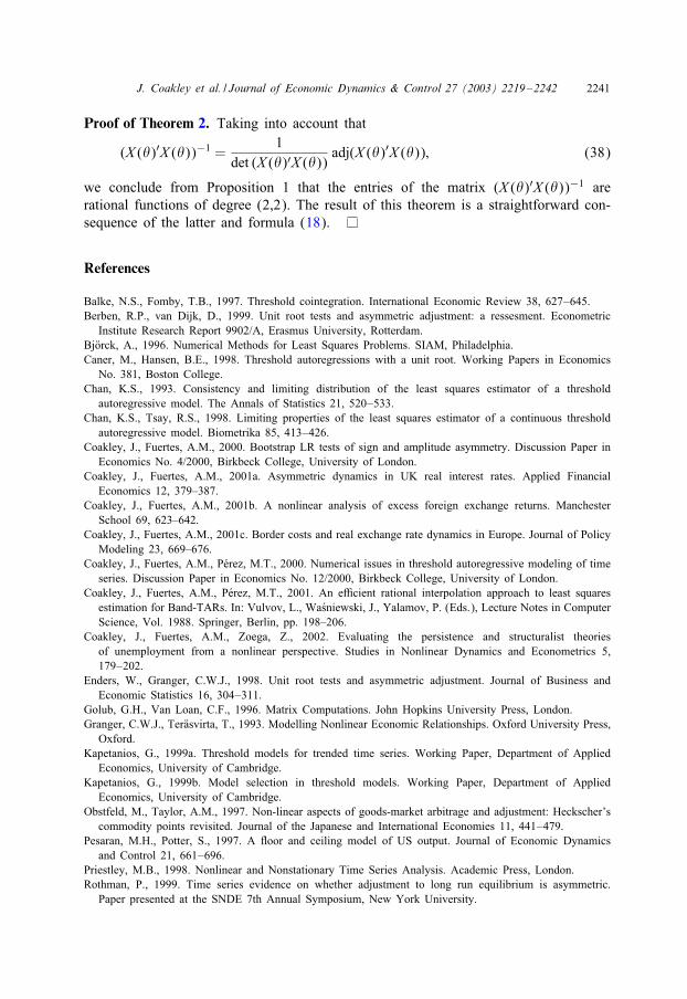
Proof of Theorem 2. Taking into account that
(X ()′X ())−1 =1
det (X ()′X ())adj(X ()′X ()); (38)
we conclude from Proposition 1 that the entries of the matrix (X ()′X ())−1 arerational functions of degree (2,2). The result of this theorem is a straightforward con-sequence of the latter and formula (18).
References
Balke, N.S., Fomby, T.B., 1997. Threshold cointegration. International Economic Review 38, 627–645.Berben, R.P., van Dijk, D., 1999. Unit root tests and asymmetric adjustment: a ressesment. Econometric
Institute Research Report 9902/A, Erasmus University, Rotterdam.BjRorck, A., 1996. Numerical Methods for Least Squares Problems. SIAM, Philadelphia.Caner, M., Hansen, B.E., 1998. Threshold autoregressions with a unit root. Working Papers in Economics
No. 381, Boston College.Chan, K.S., 1993. Consistency and limiting distribution of the least squares estimator of a threshold
autoregressive model. The Annals of Statistics 21, 520–533.Chan, K.S., Tsay, R.S., 1998. Limiting properties of the least squares estimator of a continuous threshold
autoregressive model. Biometrika 85, 413–426.Coakley, J., Fuertes, A.M., 2000. Bootstrap LR tests of sign and amplitude asymmetry. Discussion Paper in
Economics No. 4/2000, Birkbeck College, University of London.Coakley, J., Fuertes, A.M., 2001a. Asymmetric dynamics in UK real interest rates. Applied Financial
Economics 12, 379–387.Coakley, J., Fuertes, A.M., 2001b. A nonlinear analysis of excess foreign exchange returns. Manchester
School 69, 623–642.Coakley, J., Fuertes, A.M., 2001c. Border costs and real exchange rate dynamics in Europe. Journal of Policy
Modeling 23, 669–676.Coakley, J., Fuertes, A.M., P,erez, M.T., 2000. Numerical issues in threshold autoregressive modeling of time
series. Discussion Paper in Economics No. 12/2000, Birkbeck College, University of London.Coakley, J., Fuertes, A.M., P,erez, M.T., 2001. An e3cient rational interpolation approach to least squares
estimation for Band-TARs. In: Vulvov, L., Wa,sniewski, J., Yalamov, P. (Eds.), Lecture Notes in ComputerScience, Vol. 1988. Springer, Berlin, pp. 198–206.
Coakley, J., Fuertes, A.M., Zoega, Z., 2002. Evaluating the persistence and structuralist theoriesof unemployment from a nonlinear perspective. Studies in Nonlinear Dynamics and Econometrics 5,179–202.
Enders, W., Granger, C.W.J., 1998. Unit root tests and asymmetric adjustment. Journal of Business andEconomic Statistics 16, 304–311.
Golub, G.H., Van Loan, C.F., 1996. Matrix Computations. John Hopkins University Press, London.Granger, C.W.J., TerRasvirta, T., 1993. Modelling Nonlinear Economic Relationships. Oxford University Press,
Oxford.Kapetanios, G., 1999a. Threshold models for trended time series. Working Paper, Department of Applied
Economics, University of Cambridge.Kapetanios, G., 1999b. Model selection in threshold models. Working Paper, Department of Applied
Economics, University of Cambridge.Obstfeld, M., Taylor, A.M., 1997. Non-linear aspects of goods-market arbitrage and adjustment: Heckscher’s
commodity points revisited. Journal of the Japanese and International Economies 11, 441–479.Pesaran, M.H., Potter, S., 1997. A [oor and ceiling model of US output. Journal of Economic Dynamics
and Control 21, 661–696.Priestley, M.B., 1998. Nonlinear and Nonstationary Time Series Analysis. Academic Press, London.Rothman, P., 1999. Time series evidence on whether adjustment to long run equilibrium is asymmetric.
Paper presented at the SNDE 7th Annual Symposium, New York University.

2242 J. Coakley et al. / Journal of Economic Dynamics & Control 27 (2003) 2219–2242
Schlittgen, R., 1997. Fitting of threshold models for time series. Discussion Paper No. 97-13, University ofCalifornia, San Diego.
Stoer, J.F., Bulirsch, R., 1992. Introduction to Numerical Analysis. Springer, Berlin.Tong, H., 1983. Threshold Models in Non-linear Time Series Analysis. Springer, Berlin.Tong, H., Lim, K.S., 1980. Threshold autoregression, limit cycles and cyclical data. Journal of the Royal
Statistical Society B 42, 245–292.Tsay, R.S., 1989. Testing and modelling threshold autoregressive processes. Journal of the American
Statistical Association 84, 231–240.