Imperial College London

Numerical General Relativity in

Exotic Settings

Alexander Adam

December 19, 2013

Submitted in part fulfillment of the requirements for the degree of

Doctor of Philosophy in Theoretical Physics of Imperial College London

and the Diploma of Imperial College London

1

Abstract

In this thesis, we discuss applications of numerical relativity in a variety of complex

settings. After introducing aspects of black hole physics, extra dimensions, holog-

raphy, and Einstein-Aether theory we discuss how one can frame the problem of

solving the static Einstein equations as an elliptic boundary value problem by inclu-

sion of a DeTurck gauge fixing term. Having setup this background, we turn to our

simplest application of numerical relativity, namely fractionalisation in holographic

condensed matter. We explain how one may describe this phenomenon by studying

particular classes of hairy black holes and analysing whether bulk flux is sourced by

a horizon or charged matter. This problem is our simplest application of numerical

relativity as the Einstein equations reduce to ODEs and the problem may be solved

by shooting methods. We next turn to a discussion of stationary numerical relativ-

ity and explain how one can also view the problem of finding stationary black hole

solutions as an elliptic problem, generalising the static results discussed earlier. Er-

goregions and horizons are naively a threat to ellipticity, but by considering a class

of spacetimes describing a fibration of the stationary and axial Killing directions

over a Riemannian base space manifold, we show how the problem can neverthe-

less still be phrased in this manner. Finally we close with a discussion of black

holes in Einstein-Aether theory. These unusual objects have multiple horizons as a

consequence of broken Lorentz symmetry, and in order to construct such solutions

we explain how to generalise the PDE methods of previous sections to construct

solutions interior to a metric horizon where the Harmonic Einstein equations cease

to be elliptic. Using this new machinery we rediscover the spherically symmetric

static black holes that have been found in the literature and moreover present the

first known rotating solutions of the theory.

2

In loving memory of my grandmother, Ida Ciancabilla

Benocci.

3

Preface

Declaration of Originality

I declare that this thesis has been written by myself and constitutes a survey of

my own research, except in cases where references are explicitly made to the work

of others or to work that was done as part of a collaboration. In detail, the work

discussed in chapters 2 and 3 of this thesis is based on material taken from the

following publications:

❼ A. Adam, S. Kitchen, and T. Wiseman, A numerical approach to finding

general stationary vacuum black holes, Class.Quant.Grav. 29 (2012) 165002,

[arXiv:1105.6347]

❼ A. Adam, B. Crampton, J. Sonner, and B. Withers, Bosonic Fractionalisation

Transitions, JHEP 1301 (2013) 127, [arXiv:1208.3199]

All calculations presented in chapter 3 are taken from the former and were per-

formed by the present author. Chapter 2 is based on the second reference above

and all analytic calculations, as well as the T = 0 numerics were carried out by the

present author in collaboration with Crampton. Chapter 4 is based on work done

in collaboration with Wiseman and Pau Figueras that is soon to be submitted for

publication. The static calculations in this chapter (section 4.4) were also done in

collaboration with Yosuke Misonoh.

All research discussed in this thesis was carried out during the time I was registered

at Imperial College London, between October 2009 and October 2013. No part of

this work has been submitted for any other degree at this or another institution.

Acknowledgments

I wold like to thank my supervisor, Dr Toby Wiseman for his advice during my

time at Imperial College London and in particular for encouraging me to develop

my numerical skills despite much initial opposition! I would also like to thank

Professor Fay Dowker for many years of guidance and support throughout both

4

my undergraduate and postgraduate years at Imperial. Thanks are also due to

Benedict Crampton, Julian Sonner, Benjamin Withers, Sam Kitchen, Pau Figueras

and Yosuke Misonoh for enjoyable collaborations.

More thanks than I can say here are owed to my colleagues in H606 for many

enlightening and entertaining discussions over the years and for ensuring that no

day was without excitement!

I’d also like to thank particularly my parents and close friends who have provided

me with invaluable moral support whilst I’ve been carrying out my research without

which none of this would have been possible. The author is also grateful for the

financial support that has been provided under a doctoral training grant by the

Science and Technologies Facilities Council (STFC).

Copyright Declaration

‘The copyright of this thesis rests with the author and is made available under a Cre-

ative Commons Attribution Non-Commercial No Derivatives license. Researchers

are free to copy, distribute or transmit the thesis on the condition that they at-

tribute it, that they do not use it for commercial purposes and that they do not

alter, transform or build upon it. For any reuse or redistribution, researchers must

make clear to others the license terms of this work’

5

Contents

1. Gravitational Theory in Exotic Settings 11

1.1. Introduction . . . . . . . . . . . . . . . . . . . . . . . . . . . . . . . . 11

1.2. Higher Dimensional Black Holes, AdS/CFT and Holography . . . . . 13

1.2.1. Killing Fields, Static and Stationary Spacetimes . . . . . . . . 15

1.2.2. No Hair Theorems and Black Hole Uniqueness . . . . . . . . . 17

1.2.3. Black Hole Mechanics and Thermodynamics . . . . . . . . . . 20

1.2.4. Examples of Asymptotically Flat Black Holes . . . . . . . . . 26

1.2.5. Holography and the AdS/CFT Correspondence . . . . . . . . 32

1.3. Static Elliptic Numerical Relativity . . . . . . . . . . . . . . . . . . . 37

1.3.1. Ansatz for Static Black Holes . . . . . . . . . . . . . . . . . . 38

1.3.2. Hyperbolicity, Ellipticity and the Harmonic Einstein Equation 39

1.3.3. Ricci Flatness, Solitons, and Maximum Principles . . . . . . . 47

1.3.4. Numerical Implementations . . . . . . . . . . . . . . . . . . . 50

1.4. Einstein-Aether Gravity . . . . . . . . . . . . . . . . . . . . . . . . . 53

1.4.1. Action and Field Equations . . . . . . . . . . . . . . . . . . . 55

1.4.2. Wave Modes and Physical Degrees of Freedom . . . . . . . . . 60

1.4.3. Constraints on the Parameter Space . . . . . . . . . . . . . . . 65

2. Bosonic Fractionalisation in AdS/CFT 69

2.1. Introduction . . . . . . . . . . . . . . . . . . . . . . . . . . . . . . . . 69

2.2. General Features, Action and Field Content . . . . . . . . . . . . . . 72

2.3. Ultraviolet Expansions and Asymptotic Charges . . . . . . . . . . . . 77

2.4. Thermodynamics . . . . . . . . . . . . . . . . . . . . . . . . . . . . . 78

2.5. Class I: Bottom Up Model and T = 0 Shooting Problem . . . . . . . 81

2.5.1. T=0 Infrared Expansions . . . . . . . . . . . . . . . . . . . . . 82

2.5.2. Overview of the Numerical Shooting Problem . . . . . . . . . 89

2.5.3. T=0 Fractionalisation Transition . . . . . . . . . . . . . . . . 91

2.5.4. Comments on Finite Temperature . . . . . . . . . . . . . . . . 96

2.6. Class Ib: Bottom - Up Model . . . . . . . . . . . . . . . . . . . . . . 97

6

2.7. Class II: M Theory . . . . . . . . . . . . . . . . . . . . . . . . . . . . 97

2.7.1. Phase Structure . . . . . . . . . . . . . . . . . . . . . . . . . . 98

2.7.2. Neutral Top-Down Solutions . . . . . . . . . . . . . . . . . . . 99

2.8. Discussion . . . . . . . . . . . . . . . . . . . . . . . . . . . . . . . . . 102

3. Stationary Elliptic Numerical Relativity 104

3.1. Introduction . . . . . . . . . . . . . . . . . . . . . . . . . . . . . . . . 104

3.2. Static Spacetimes from a Lorentzian Perspective . . . . . . . . . . . . 105

3.3. Stationary Spacetimes with Globally Timelike Killing Vector . . . . . 110

3.4. Stationary Black Holes . . . . . . . . . . . . . . . . . . . . . . . . . . 114

3.4.1. Ellipticity of the Harmonic Einstein Equation . . . . . . . . . 116

3.4.2. Reduced Stationary Case . . . . . . . . . . . . . . . . . . . . . 118

3.4.3. Horizon and Axis Boundaries . . . . . . . . . . . . . . . . . . 119

3.5. Example of Boundary Conditions: Kerr . . . . . . . . . . . . . . . . . 123

3.6. Discussion . . . . . . . . . . . . . . . . . . . . . . . . . . . . . . . . . 126

4. Black Holes in Einstein-Aether Theory 128

4.1. Introduction . . . . . . . . . . . . . . . . . . . . . . . . . . . . . . . . 128

4.2. Structure and Regularity of Einstein-Aether Black Holes . . . . . . . 131

4.3. Ingoing Stationary Methods . . . . . . . . . . . . . . . . . . . . . . . 133

4.4. Spherically Symmetric Black Hole Solutions . . . . . . . . . . . . . . 135

4.5. Stationary Black Hole Solutions . . . . . . . . . . . . . . . . . . . . . 148

4.6. Discussion . . . . . . . . . . . . . . . . . . . . . . . . . . . . . . . . . 163

5. Conclusions and Summary 173

Appendix A. Boundary Conditions for Horizons and Axes 177

A.1. Regularity and smoothness at a Killing horizon . . . . . . . . . . . . 178

A.2. Axis of rotation . . . . . . . . . . . . . . . . . . . . . . . . . . . . . . 180

Appendix B. Connection Components and Flow Equations 181

7

List of Figures

2.1. T = 0 phase structure of the fractionalisation models of chapter 2 . . 73

2.2. Full shooting solutions for an (almost) fully fractionalised phase found

using the methods described in the main text. The solution displayed

is for Φ1/µ = 0.607. . . . . . . . . . . . . . . . . . . . . . . . . . . . . 92

2.3. Full shooting solutions for a partially fractionalised phase found using

the methods described in the main text. The solution displayed is for

Φ1/µ = 0.0964. . . . . . . . . . . . . . . . . . . . . . . . . . . . . . . 93

2.4. Full shooting solutions for a cohesive phase found using the methods

described in the main text. The solution displayed is for Φ1/µ = −0.598. 94

2.5. Dependence of the T = 0 domain walls on the parameter Φ1/µ with

shades of red indicating broken symmetry . . . . . . . . . . . . . . . 95

2.6. M-theory phase diagram showing the existence of bulk solutions at

fixed mass . . . . . . . . . . . . . . . . . . . . . . . . . . . . . . . . . 99

4.1. Profiles of the metric, aether and constraint functions for a spherically

symmetric static aether black hole withN = 12 points, c1 = 0.4, c2 =

−0.0727, c3 = 0, c4 = 0 and mass 2GMADM = 1.03(3) . . . . . . . . 142

4.2. Plot of φ = ξµξµ for the static Einstein aether black hole of Figure

4.1. This function would be a constant in the latter . . . . . . . . . . 143

4.3. Plot to constrast static black holes in Einstein-Aether theory and

general relativity. This function would be a constant in the latter . . 144

4.4. Metric functions of a static spherically Einstein-Aether black hole

constructed by shooting methods . . . . . . . . . . . . . . . . . . . . 146

4.5. Demonstration of the equivalence of our static Einstein-Aether black

holes solutions found by spectral techniques and those found by shoot-

ing methods that exist in the literature. . . . . . . . . . . . . . . . . . 147

4.6. Metric functions of a stationary Einstein-Aether black hole computed

using 6th order finite differencing from initial data and reference met-

ric with M = 1, a = 0.3, on an Nz × Nθ = 20 × 20 grid, with

c1 = 0.4, c2 = −0.0727, c3 = c4 = 0 (I) . . . . . . . . . . . . . . . . 156

8

4.7. Metric functions of a stationary Einstein-Aether black hole computed

using 6th order finite differencing from initial data and reference met-

ric with M = 1, a = 0.3, on an Nz × Nθ = 20 × 20 grid, with

c1 = 0.4, c2 = −0.0727, c3 = c4 = 0 (II) . . . . . . . . . . . . . . . 157

4.8. Aether and constraint functions of a stationary Einstein-Aether black

hole computed using 6th order finite differencing from initial data and

reference metric with M = 1, a = 0.3, on an Nz ×Nθ = 20× 20 grid,

with c1 = 0.4, c2 = −0.0727, c3 = c4 = 0. . . . . . . . . . . . . . . . 158

4.9. Plot of 1− S(z,θ=0)B(z,θ=0)

to check axis regularity for the stationary aether

black hole described in the text with c1 = 0.4, c2 = −0.0727, c3 =

c4 = 0 on a Nz × Nθ = 20 × 20 grid. We see that as required by

regularity, this quantity is consistent with being zero. . . . . . . . . . 159

4.10. Mass of the stationary aether black holes discussed in the text as a

function of c1, with c2 chosen so that the metric and spin-0 horizons

coincide and c3 = c4 = 0. . . . . . . . . . . . . . . . . . . . . . . . . . 159

4.11. Angular momentum per unit mass of the stationary aether black holes

discussed in the text as a function of c1, with c2 chosen so that the

metric and spin-0 horizons coincide and c3 = c4 = 0. . . . . . . . . . . 160

4.12. Plot of the proper size of the metric, spin-1 and spin-2 horizons in

the equatorial plane (θ = π/2) for the stationary aether black holes

discussed in the text as a function of c1. The corresponding quantity

for a Kerr black hole of the same mass (for a given c1) is also shown. 161

4.13. Low resolution plot of the maximum value of φ = ξµξµ as a function

of grid size for the black hole described in the text found using 6th

order finite differencing. . . . . . . . . . . . . . . . . . . . . . . . . . 164

4.14. Low resolution plot of the maximum value of φ = ξµξµ as a function of

grid size for the black hole described in the text found using spectral

differencing. . . . . . . . . . . . . . . . . . . . . . . . . . . . . . . . . 165

4.15. High resolution plot of the maximum value of φ = ξµξµ as a function of

grid size for the black hole described in the text found using 6th order

finite differencing. We see indication of convergence to a solution with

vanishing ξ. . . . . . . . . . . . . . . . . . . . . . . . . . . . . . . . . 166

4.16. High resolution plot of the maximum value of |φ| = |ξµξµ| as a func-

tion of grid size for the black hole described in the text found using

spectral differencing. There is no convergence and spectral methods

fail for this problem. . . . . . . . . . . . . . . . . . . . . . . . . . . . 167

9

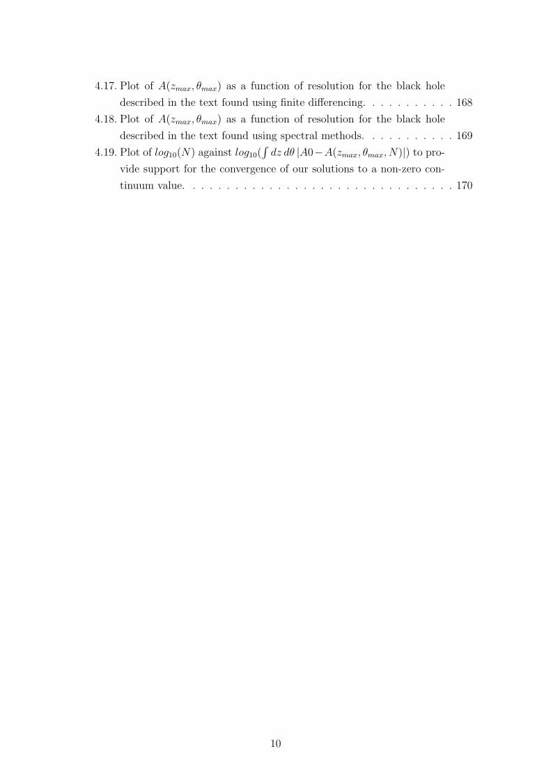
4.17. Plot of A(zmax, θmax) as a function of resolution for the black hole

described in the text found using finite differencing. . . . . . . . . . . 168

4.18. Plot of A(zmax, θmax) as a function of resolution for the black hole

described in the text found using spectral methods. . . . . . . . . . . 169

4.19. Plot of log10(N) against log10(∫dz dθ |A0−A(zmax, θmax, N)|) to pro-

vide support for the convergence of our solutions to a non-zero con-

tinuum value. . . . . . . . . . . . . . . . . . . . . . . . . . . . . . . . 170

10

1. Gravitational Theory in Exotic

Settings

1.1. Introduction

Einstein’s theory of General Relativity has revolutionised our understanding of the

universe, and stands as one of the greatest achievements of modern physics. The

mathematical structure of the theory is however rather complex and nearly a cen-

tury after its inception, only a handful of exact solutions to the Einstein field equa-

tions have been discovered, rendering numerical techniques invaluable. Numerical

relativity has since become an extremely diverse field, its usefulness continuing to

increase with the dramatic rise in modern computing power. Today the subject has

a plethora of remarkable applications ranging from simulations of neutron star struc-

ture and the relativistic fluid dynamics of supernova explosions though to the study

of gravitational radiation from phase transitions in the early universe [3, 4, 5, 6].

In addition to these astrophysical and cosmological applications, numerical general

relativity has become invaluable in fundamental theoretical physics, notably quan-

tum gravity. In this arena, studies of black holes have shed light on various unusual

aspects of strongly coupled gauge theories and matrix theories, many of which are

of direct relevance to condensed matter physics [7, 8, 9, 10, 11]. In turn, studies of

the latter have began to yield insights into open questions relating to the thermody-

namics of horizons and unitarity in black hole evaporation [12, 13, 14, 15, 16]. The

study of exotic black holes serves as the unifying theme of this thesis, whether in

the context of dual descriptions of quantum field theories, cosmologically interesting

models of gravitational Lorentz symmetry breaking or simply to elucidate the rather

striking phase structure of gravity in higher dimensions.

In the remainder of this chapter, we will turn to a survey of some of the topics

outlined above. In section 1.2, we shall provide an overview of aspects of black holes

in higher dimensions and how they differ from their four dimensional counterparts.

We will also introduce holography and the famous AdS/CFT correspondence. Orig-

inating in the work of t Hooft, [17] and finding its first explicit realisation in string

11

theory, [18] this striking result relates gravitational physics in a given dimension to

a quantum field theory in (at least) one dimension lower. We take a relativist’s per-

spective where the emphasis is on gravitational aspects of the correspondence and

the key role played by black holes. Given the difficulty in finding analytic solutions

in gravitational theories (particularly in higher dimensions or when coupled to ex-

otic matter), we move in section 1.3 to a discussion of elliptic methods for numerical

relativity. Although the full Einstein equations constitute a complicated hyperbolic

system, in many static and stationary scenarios, if only the solution exterior to a

horizon is required, one can recast the problem in a rather different way. In fact,

by inclusion of a DeTurck gauge fixing term [19], the system becomes an elliptic

boundary value problem that can be solved by standard numerical algorithms such

as the Newton method, using only desktop computing resources [20, 21]. Much of

the remainder of the thesis will constitute an application of a generalisation of these

techniques to exotic stationary black holes. Finally in section 1.4 we change direction

somewhat to introduce an unusual modification of gravity, known as Einstein-Aether

theory. This theory is consistent with all current observational constraints and dif-

fers from general relativity in that it spontaneously breaks Lorentz symmetry by the

inclusion of a dynamical timelike vector field, introducing a preferred frame in the

universe [22, 23, 24]. The consequences of this for black hole theory will be discussed

in detail in the final chapter of this thesis.

The main body of this thesis is divided into three chapters. Chapter 2, contains

our simplest application of numerical relativity - this is in the area of AdS/CFT

where we show how to construct gravitational duals to ‘fractionalisation transitions’

in condensed matter. As we shall discuss, the problem amounts to constructing

a family of static neutral and charged black holes with and without scalar hair.

Since these black holes are static, the Einstein equations become ordinary differ-

ential equations (ODEs) and the full machinery of elliptic numerical relativity is

not required. We proceed by more conventional shooting methods to construct the

solutions and discuss their physical implications. We briefly comment on extensions

of this work however involving ‘striped’ phases where the equations become partial

differential equations (PDEs) and the full technology of elliptic numerical relativity

could prove extremely useful. In chapter 3 we discuss how to generalise the tech-

niques of section 1.3 to the case of stationary (rather than static) situations. We will

discuss this construction in detail, paying attention in particular to the boundary

conditions required for the PDE system to be regular at any horizons and axes of

symmetry. In the final part of this thesis, chapter 4 we discuss the rather peculiar

black holes that exist in Einstein-Aether theory. As a consequence of the broken

12

Lorentz symmetry in the theory, these solutions have several horizons corresponding

to trapping gravitational and aether perturbations of different spin. We discuss an

extension of the stationary techniques of chapter 3 that uses ingoing Eddington-

Finkelstein coordinates to construct the interior black hole solution by solving a

mixed hyperbolic-elliptic system. This is an important ingredient, as we will need

to be able to construct the solution interior to the metric horizon in order to fully

display the exotic structure of these black holes. We discuss in detail how to con-

struct the static solutions in the literature by completely different techniques and

then proceed to present the first known (general) rotating solutions of the theory.

1.2. Higher Dimensional Black Holes, AdS/CFT

and Holography

Originally thought to be mere mathematical curiosities, it is now almost certain

that black holes exist in our universe (see e.g. [25]). With the advent of string/M

theory, it has become natural to extend one’s study of physics to higher dimensions

and hence to investigate also black holes in dimensions D > 4. The study of these

solutions is given even greater weight by certain models with TeV scale gravity where

such black holes may turn out to be observable at the LHC and the next generation of

supercolliders, potentially providing a window into Planck scale physics [26, 27, 28].

Even more remarkable is that by virtue of the AdS/CFT correspondence, some of

these higher dimensional solutions may be of relevance to the quark-gluon plasma

in particle physics, [29, 30, 31, 32] and strikingly as mentioned previously, even to

low energy condensed matter physics.

In this section, we provide an overview of black hole physics in four and higher di-

mensions, discussing the concepts of Killing vectors, isometries, no-hair and unique-

ness theorems as well as some of the famous analytic vacuum solutions that have

been obtained. We shall also introduce aspects of Euclidean quantum gravity and

its relationship to black hole radiation and thermodynamics. Holography and the

AdS/CFT correspondence are then introduced and a survey of the ‘holographic dic-

tionary’ is given, where the central role played by black holes in the construction of

holographic duals becomes apparent.

Black holes are a particular class of solutions to the Einstein equations, which

are most elegantly obtained by way of a variational principle. In the second order

formalism that we employ throughout this thesis, the metric is the (gravitational)

dynamical variable and the relevant action coupled to matter contains (in its most

general form) an Einstein-Hilbert term SEH [g] , a Gibbons-Hawking boundary term

13

SB[g], a non-dynamical term S0 and finally (in non-vacuum settings) a contribution

from the matter action SM [g, ψ] [33]. Working in (−,+,+,+) signature and in units

where the speed of light c = 1 we have

S[g, ψ] = SEH [g] + SB[g]− S0 + SM [g, ψ] ,

SEH [g] =1

16πG

∫

V

√−g R ,

SB[g] =1

8πG

∫

∂V

√

|h| ǫK ,

S0 =1

8πG

∫

∂V

√

|h| ǫK0 ,

SM [g, ψ] =

∫

V

√−gLM(ψ) , (1.2.1)

where V denotes some submanifold of the spacetime manifold M. R is the Ricci

scalar, h is the determinant of the induced metric on ∂V (the boundary of V) andK is

the trace of the extrinsic curvature of ∂V . The quantity K0 is the extrinsic curvature

of ∂V embedded in flat space as we shall discuss below. With our conventions

(defined above (1.2.1)), the numerical factor ǫ is +1 when ∂V is timelike and −1

when ∂V is spacelike.

The Gibbons-Hawking term must a-priori be included when M is a manifold with

boundary, to ensure well-posedness of the associated Dirichlet variational problem,

where the induced metric on this boundary is held fixed. It turns out to have physical

relevance as well, contributing to the on shell action and hence the thermodynamics

of gravitational solutions. The term S0 affects only the numerical value of the

action and does not contribute to local dynamics. It should nevertheless be included

formally when M is non-compact to regularise the total gravitational action, which

is otherwise divergent. (When M is compact, this term is unnecessary). As a

simple example of such a contribution, an appropriate choice for asymptotically flat

spacetimes (which results in zero action for flat space) is obtained as mentioned

above, by taking K0 to be the extrinsic curvature of ∂V embedded in flat space1.

Finally, the action SM [g, ψ] may be used to couple any desired matter fields ψ to

the system. Examples could include standard model fields or more exotic matter

contributions motivated by string theory reductions, the latter in particular playing

a role in holography as we shall see in chapter 2.

1The choice of K0 is tantamount to a choice of regularisation scheme for the gravitational actionand the choice we have just mentioned, useful for asymptotically flat spacetimes, is of coursenot the only possibility. In particular, for asymptotically AdS spacetimes that we discuss laterin the context of holography in section 1.2.5 and chapter 2, the terms that one must add torenormalise the on shell action are more complex. See for instance [34].

14

The Einstein field equations are obtained on varying the total action (1.2.1) with

respect to the metric, subject to the condition that δgµν |∂V = 0. In our conventions

they take the form

Rµν −1

2gµνR = 8πGTµν , (1.2.2)

where Tµν = − 2√−gδ(√−gLM )δgµν is the stress energy tensor. For the remainder of this

section we discuss the general characteristics of black hole solutions of these equa-

tions.

Heuristically, a spacetime (M, g) is said to contain a black hole if there exist

outgoing null geodesics within it that never reach future null infinity J +. This

motivates the formal definition of the black hole region B of some spacetime manifold

M as the set of points that do not belong to the causal past of future null infinity

B = M− J−(J +) . (1.2.3)

This definition mathematically captures the famous statement that a black hole is

a region of spacetime from which light and timelike observers cannot escape. The

boundary ∂ between the black hole region and the rest of the manifold serves as a

‘surface of no return’ and defines the black hole event horizon H,

H = ∂B = ∂(J−(J +)) , (1.2.4)

(where we have assumed that M itself has no boundary).

The equations (1.2.3), (1.2.4) above define precisely what is meant by a black

hole and its horizon in term of global causal structure. In this thesis, we will be

concerned for the most part only with the local properties of solutions to the Einstein

equations and further global definitions of singularities, and horizons will therefore

not be required in what follows. The above definitions are nevertheless included for

completeness and further such details may be found in [35, 36].

1.2.1. Killing Fields, Static and Stationary Spacetimes

The Einstein equations are a complicated system of nonlinear partial differential

equations and non-trivial exact solutions are in general very difficult to find. It

will be convenient in discussing black hole solutions to use symmetries to classify

different spacetimes and this motivates the introduction of Killing vectors. In this

section we follow [33].

A tensor T α...β... is said to be Lie transported along a curve C (parameterised by λ)

15

if its Lie derivative along C is zero: LuTα...β... = 0 where uα = dxα/dλ is the curve’s

tangent vector. If adapted co-ordinates are now chosen such that only x0 ≡ λ varies

on C, it follows that uα.= δα0 and hence that ∂βu

α .= 0. (The symbol

.= denotes

equality in the specified coordinate system). One then has that LuTα...β...

.= T α...

β...,µuµ .=

∂∂x0T

α...β... = 0 and consequently the tensor’s components are all independent of x0 in

the chosen coordinate system. Conversely, it can be shown that if in some coordinate

system the components of a tensor do not depend on some coordinate y, the Lie

derivative of the tensor in the direction ∂/∂y will vanish.

As a consequence of the discussion above, if there exists a coordinate system in

which the components of the metric do not depend on one of the coordinates, it

follows that Lξgαβ = 0. The associated vector field ξα is called a Killing vector field

and is a generator of isometries (diffeomorphisms of the metric). The condition

that a vector field be Killing is known as Killing’s equation and is most conveniently

written as

Lξgαβ = ∇αξβ +∇βξα = 0 , (1.2.5)

where the definition of the Lie derivative in terms of the covariant derivative as well

as metric compatibility ∇γgαβ = 0 have been used.

Having defined Killing vectors, it is useful to introduce the notion of a Killing

horizon. A Killing horizon is a hypersurface in a spacetime (M, g) on which the

norm of a Killing vector goes to zero. Equivalently, a null hypersurface Σ, (that is to

say a hypersurface with a null normal vector), is a Killing horizon of a Killing vector

field ξα if the latter is normal to Σ. It is in general not the same region as the event

horizon although for certain classes of spacetime (notably the stationary spacetimes

we introduce below) these regions can coincide. Notice the marked difference in the

definitions of these two different horizons - an event horizon is introduced in terms

of global causal structure, whilst a Killing horizon can be understood in terms of

local coordinates. We may now proceed to classify different spacetimes according to

their isometries.

An asymptotically flat spacetime is said to be stationary if it admits a Killing vec-

tor field k which is timelike in a neighbourhood of J ±. By the considerations above,

this implies that there exists a coordinate system in which the metric coefficients

are independent of the time coordinate t, gαβ,t.= 0 with k = ∂/∂t.

A stationary spacetime is also static if the timelike Killing field k is hypersur-

face orthogonal. That is to say, if the spacetime admits a foliation (heuristically a

‘slicing’) into hypersurfaces such that the Killing field k is everywhere orthogonal

to these surfaces. Frobenius’s theorem gives the necessary and sufficient condition

16

for hypersurface orthogonality, namely that a given vector field uα is hypersurface

orthogonal if and only if u[α;βuγ] = 0 [35]. It can be shown that this is equivalent

to the statement that the vector field is irrotational and one may further rephrase

this as the requirement that the metric (written in coordinates adapted to the static

symmetry) is invariant under time reversal symmetry t → −t and hence contains

no off diagonal time pieces. We finally reiterate that for static spacetimes, the event

and Killing horizons coincide, a fact that can be used to obtain global information

about the spacetime (the event horizon) from local information (the Killing horizon)

and is very useful in practice to locate the event horizon.

A spacetime is said to be axisymmetric if,

1. It admits a Killing vector field m that is spacelike in a neighbourhood of J ±.

2. The Killing field m generates a one-parameter group of isometries isomorphic

to U(1).

A spacetime is both stationary and axisymmetric if it simultaneously satisfies the

definitions of stationarity and axisymmetry and in addition satisfies [k,m] = 0.

One conventionally chooses adapted coordinates for such spacetimes with m = ∂∂t

and k = ∂∂φ

where φ is identified with period 2π. Such stationary solutions are of

great importance in physics as they approximate the exterior gravitational field of

rotating bodies and are consequently of relevance in astrophysics. We will shortly

return to these classes of spacetimes in the context of uniqueness theorems for black

holes where we introduce the Rigidity Theorem, a result that plays an important

role in our work in chapter 3.

1.2.2. No Hair Theorems and Black Hole Uniqueness

Before presenting particular black hole solutions in four and higher dimensions, we

discuss further some general results in black hole theory. In this section we introduce

the notions of black hole uniqueness and the related ‘no hair’ theorems. Further de-

tails may be found in the reviews [37, 38, 39, 40]. ‘No hair’ refers to the property

that the space of all black hole solutions in a given dimension is parameterised by

a (small) number of asymptotically measured quantities. In this sense, a black hole

is very different from a star or for that matter from a speculative ultra compact

remnant of gravitational collapse. Such objects would require an arbitrarily large

number of multipole moments to specify their states and the remarkable physical

content of the no hair theorems is that almost all of this additional information is

‘lost’2 during gravitational collapse to form a black hole. In D = 4, it has been

2Some of the information is likely radiated away to infinity during collapse in the form of gravita-tional waves, but a portion inevitably also falls within the horizon when it forms and remainstrapped inside the black hole forever (at least at the classical level).

17

shown, (see for example [41, 42]), that only four parameters are required to com-

pletely specify a black hole state: the massM , angular momentum J , electric charge

Q and magnetic charge P 3. These are further known to correspond to conserved

quantities. In higher dimensions, it is still believed to be true that a black hole can

be completely specified by a small number of parameters [39], but the existence of

non conserved dipole charges in the D = 5 rotating black ring solution of [44, 45],

(discussed briefly in section 1.2.4) explicitly demonstrates that these parameters

need no longer correspond to conserved charges when D > 4.

Black hole uniqueness refers to a property of the space of black hole solutions

whereby specification of a given set of asymptotic parameters (as defined above

with regards to the no hair theorem) selects a unique black hole as opposed to

some collection of black holes. In D = 4, uniqueness has been proven, although the

proof relies heavily on results that are very specific to D ≤ 4. In particular, the

Hawking black hole topology theorem which guarantees that spatial cross sections

of the event horizon in D = 4 are topologically S2 is crucial in the proof. This result

makes use of the Gauss-Bonnet theorem (valid in two dimensions) to prove that the

two dimensional spatial cross sections of the horizon are spherical/toroidal, followed

then by a topological argument to eliminate the toroidal possibility [36]. These

results have been strengthened by Chrusciel and Wald using topological censorship

[46] which states that in an asymptotically flat and globally hyperbolic spacetime

obeying the null energy condition, any causal curve that starts and ends at infinity

can be continuously deformed to infinity. Although this result holds for all D, the

topological restrictions it implies are only strong for D < 4, and little extra is gained

in D > 4 [39].

In higher dimensions, it is known from the above discussion that the topological

restrictions on the horizon are relaxed and there are several examples of black hole

solutions (see sections 1.2.4, 1.2.4) that explicitly demonstrate that non spherical

event horizons are possible. Moreover one finds that black hole uniqueness does not

in general hold in higher dimensions. (There are some specific uniqueness results for

D > 4, static, asymptotically flat spacetimes which are discussed briefly below, but

general uniqueness no longer holds). The breakdown of the uniqueness theorems

implies the existence of a nontrivial phase diagram where a variety of black hole

phases can coexist with the same asymptotic charges. In principle, there could be

3In making this statement, we have implicitly assumed that we are considering Einstein-Maxwelltheory in asymptotically flat spacetimes. Even in flat space in D = 4, the situation is differentif one allows Yang-Mills fields (see e.g. [43]) and black holes with non-Abelian hair becomepossible. Note also that even though we restrict our discussion here to asymptotically flatspacetimes, in section 1.2.5 we briefly mention how black hole uniqueness fails in asymptoticallyAdS space, allowing for black holes with scalar hair there.

18

phase transitions between the different regions of the diagram, and it is therefore of

interest to know which phases are entropically favoured in a given dimension and in

a given range of parameter space, a topic of considerable importance in applications

of holography.

The breakdown of black hole uniqueness in D > 4 leaves a plethora of exotic

higher dimensional solutions. Classification and solution generating techniques (e.g.

the Petrov classification and Newman-Penrose formalism [47]) valid in D = 4 do

not readily generalise to D > 4 and hence a full higher dimensional, analytic clas-

sification of solutions may be impossible, highlighting the importance of numerical

relativity in these settings. We now discuss in more detail some specific uniqueness

and no hair results and introduce some of the analytic black hole solutions in D

dimensions.

In D = 4, spherically symmetric vacuum solutions of the Einstein’s equations are

static and asymptotically flat. This result is known as Birkhoff’s theorem [36, 48].

There is further a theorem due to Israel, Bunting and Masood that states that if

(M, g) is a static, asymptotically flat vacuum spacetime, non-singular on and outside

an event horizon, then (M, g) is the Schwarzchild metric [49, 50]. This proves that

static, vacuum, multi black hole solutions do not exist and that Schwarzchild is the

unique spherically symmetric, asymptotically flat, vacuum black hole. Physically,

Birkhoff’s theorem implies that the gravitational field outside a pulsating sphere

remains Schwarzchild at all times and hence there is no monopole gravitational

radiation. These results extend to higher dimensions D > 4, and the associated

generalisation of the Schwarzchild solution is called a Schwarzchild-Tangherlini black

hole and has analogous uniqueness properties [39, 51].

In the case of Einstein-Maxwell theory, there exists a generalisation of the Birkhoff

result which proves that spherically symmetric, asymptotically flat, electrovacuum

black holes must be Reissner-Nordstrom (RN), if one restricts to non-degenerate

event horizons or either RN or one of the Majumdar-Papapetrou multi RN solutions

if one allows degenerate horizons [52]. In principle, the above theorems allow a

complete classification of static electrovacuum black holes in any dimension.

For stationary spacetimes in D = 4, there is a theorem due to Hawking and Wald

that states that if (M, g) is a stationary, non-static, asymptotically flat solution of

the Einstein-Maxwell equations that is non-singular on, and outside, a connected

event horizon then,

1. (M, g) is axisymmetric

2. The event horizon is a Killing horizon of ξ = k + ΩHm for some ΩH 6= 0.

19

where as before in adapted coordinates, the Killing vectors k = ∂/∂t and m = ∂/∂φ.

This important result known as the (Strong) Rigidity Theorem proves that for

black holes, stationary =⇒ axisymmetric [36, 40]. (Notice that in the static

case, it also proves our previous claim that the Killing and event horizons coincide).

The physical interpretation of the rigidity theorem is that the horizon of a rotating

stationary black hole is generated by an isometry of the spacetime itself. One could

envision a situation where there was rotation in a direction that is not an isometry,

but then physically we would expect such a solution to emit gravitational radiation,

and thus cease to be stationary. There is also a further theorem relevant in the

stationary case due to Carter, Mazur and Robinson [41, 42, 53] that states that if

(M, g) is an asymptotically flat, stationary, electrovacuum spacetime, non-singular

on and outside a connected event horizon, then (M, g) is a member of the four-

parameter (M,J,Q, P ) Kerr-Newman family.

The rigidity theorem has been extended to higher dimensions and guarantees the

existence of at least one rotational isometry [54, 55]. Curiously all the known analytic

higher dimensional stationary solutions such as the Myers-Perry black holes and the

Emparan-Reall black rings however have more than just a single such rotational

isometry. For a long time, it was unclear whether this result was always true in

higher dimensions or whether it was merely a reflection of our inability to find

solutions with little symmetry due to the extreme complexity of the equations [39].

Recently, however there has been work on constructing perturbations to the near

horizon geometries of Myers-Perry black holes, that preserve only a single rotational

isometry and nothing more [56, 57, 58]. One can use these perturbations to generate

new branches of (numerical) black hole solutions that demonstrate that there are

indeed higher dimensional black holes with less symmetry. In any event, it is clear

that the stationary case is much less constrained than the static case and a full

theoretical classification of higher dimensional stationary black holes remains elusive.

1.2.3. Black Hole Mechanics and Thermodynamics

Quite remarkably, it was shown in the 1970s, that classical black holes obey a set of

equations analogous to the four laws of thermodynamics [59]. These laws of black

hole mechanics are rigorous mathematical results that follow only from the Einstein

equations, and the energy conditions on the spacetime matter content [35, 36]. In

this section we briefly outline these laws and their striking implications.

The zeroth law of black hole mechanics states that for a stationary black hole, a

quantity known as the surface gravity κ is constant across the event horizon (where

20

the latter is a Killing horizon of the vector ξ = κ+ΩHm that was defined previously)

κ = const . (1.2.6)

The surface gravity κ may be interpreted as the force required of an observer at

∞ to keep a particle of unit mass stationary at the event horizon. Physically the

local acceleration of a test body at the event horizon diverges, but the gravitational

redshift factor goes to zero. The surface gravity is heuristically a product of the two

where the limit is well defined and it can be elegantly written in the form

κ2 = −1

2tα;βtα;β|H , (1.2.7)

where tα is the normalised tangent to the null geodesic generators of the horizon

[33]. It is important to emphasise that surface gravity is only a well defined concept

for stationary black holes as they have Killing horizons, a matter we shall return to

shortly.

The first law of black hole mechanics relates changes in the mass δM of a black

hole to changes in the area δA of its event horizon, angular momentum δJ , and

charges δQa, where the latter arise from the matter theory to which gravity is

coupled, (an example being the electric charge of Einstein-Maxwell theory)

δM =κ

8πδA+ ΩHδJ + φaδQa . (1.2.8)

In the equation above, κ and ΩH are the surface gravity and angular velocity of

the horizon respectively, and the φa are the potentials associated to the conserved

charges Qa. (In the Einstein-Maxwell theory example, a = 1 and there is a single φ

‘conjugate’ to the conserved U(1) electric charge that physically measures the electric

potential difference between the event horizon and spacelike infinity i0). The first

law holds for stationary black holes, that is to say, processes where the initial state

of the system is a stationary black hole, and the final state is a stationary black

hole. (The analogy in thermodynamics is that of a quasistatic process, where the

initial and final states are both in equilibrium).

It is important to stress at this point that both the zeroth and first laws of black

hole mechanics are non-dynamical statements that hold (as stated) only for station-

ary solutions. As alluded to above, the technical reason behind this restriction is

that the classical proofs of the theorems use the properties of Killing horizons and

whilst the event horizons of stationary black holes are guaranteed to be Killing by

the rigidity theorem, this is not true for dynamical spacetimes. There is however

21

a body of work on attempts to generalise the zeroth and first laws to dynamical,

non-equilibrium situations. This is of considerable physical interest as essentially

all realistic (astrophysical or collider) scenarios involving black holes will inevitably

be fully dynamical. One is led to introduce the concepts of isolated and dynamical

horizons, which allows progress to be made in this regard, but much still remains

unanswered - there is as of yet no conclusive notion of surface gravity in such situ-

ations for example (see for instance [60, 61]).

In contrast to the zeroth and first laws, the second law of black hole mechanics

constrains the possible dynamical evolution of black holes (e.g. black hole mergers)

and states that the total area of event horizons is non-decreasing

δA ≥ 0 . (1.2.9)

This law is also known as Hawking’s area theorem and can be proved by application

of the Raychaudhuri equation to the null geodesic congruence that generates the

horizon. It assumes only that matter obeys the weak energy condition, and in

particular is a fully dynamical statement, that does not require a notion of Killing

horizon. (That the event horizon is a null surface, can be seen from considerations

of causal structure alone).

Finally, the third law of black hole mechanics states that the so called extremal

limit of black holes, corresponding to vanishing surface gravity κ = 0 cannot be

reached in finite time by any physical process [62]. (Again, extremality is defined

with respect to stationary equilibrium black holes such that κ is defined).

It was later shown by Hawking in the framework of quantum field theory in curved

spacetime that this similarity between black hole mechanics and thermodynamics

is more than an analogy and that quantum black holes radiate as thermodynamic

objects with an associated temperature. In the case of a static black hole, this takes

the form

TH =κ

2π, (1.2.10)

(where the Planck and Boltzmann constants have been set to unity) [63]. Motivated

by the suggestive appearance of the Hawking area theorem, Bekenstein had previ-

ously conjectured that the entropy of a black hole is proportional to its horizon area

[64]. With this identification, together with Hawking’s derivation of a temperature,

the laws of black hole mechanics are in effect the laws of thermodynamics4. One

4Hawking’s identification of black hole mechanics with black hole thermodynamics also fixes theconstant of proportionality relating the black hole entropy to the horizon area as S = A

4 .

22

of the major outstanding problems in quantum gravity research is to shed light on

the underlying microstates that account for this black hole entropy, a question that

has at least partially been answered for supersymmetric black holes in string theory

[65], and constitutes one of the great triumphs of that theory.

Hawking’s original derivation uses canonical techniques and is fully Lorentzian in

character. In the remainder of this section, however we shall outline an equilibrium

derivation that uses the Euclidean path integral formulation and corresponds to

considering the canonical ensemble for gravity [66, 67]. We will show through the

example of a static black hole how the temperature may be computed directly from

the metric.

Euclidean Quantum Gravity is defined by the Feynman path integral

Z =

∫

DgDφ e−I[g,φ] , (1.2.11)

where the Euclidean action I is related to the Lorentzian action I by I = −iI.Equation (1.2.3) is in fact rather difficult to define technically as the measure on

the space of metrics Dg is generically ill defined. Moreover, the integral is divergent

as is commonplace in quantum field theory and a regularisation and renormalisa-

tion procedure is required to make sense of this fact [67]. It is expected that the

dominant contribution to the integral will come from a saddle point of the action,

corresponding to a solution of the classical field equations if one exists. (It can be

argued that this must be the case in order to recover classical general relativity in

an appropriate limit). In such a saddle point approximation, the action is expanded

as a Taylor series about background fields g0 and φ0

I[g, φ] = I[g0, φ0] + I2[g, φ] + ... , (1.2.12)

where gab = g0ab + gab, φ = φ0 + φ and I2[g, φ] is quadratic in the fluctuations g and

φ. The path integral then takes the form

logZ = −I[g0, φ0] + log

∫

DgDφ eI2[g,φ] + . . . , (1.2.13)

where the first term is physically the contribution from the background fields, and

the second term encodes one-loop quantum corrections around this background.

Since I2[g, φ] is quadratic in fluctuations, the one loop term is a Gaussian inte-

gral and may be evaluated exactly to arrive at a one-loop determinant. The latter

technically requires a regularisation procedure to be well defined (generally dimen-

sional regularisation or zeta function regularisation) but this will not be needed

in the discussion that follows (see [67] for the full calculation of this term). The

reason for this is that (1.2.13) is in fact a derivative expansion in ‘l2p∂2’ where lp

23

is the Planck length and ∂2 denotes terms with two derivatives of the metric5. In

a ‘semi-classical’ limit, where ‘higher derivatives’ are small (being irrelevant), all

one loop (and higher) quantum corrections are hence suppressed compared to the

leading term. All that remains therefore is to evaluate the dominant contribution to

logZ, namely the Euclidean action evaluated on a classical solution to the Einstein

equations. The simplest non-trivial example would be to compute the action for

the Euclidean, static, vacuum (φ0 = 0) Schwarzchild metric, but it is instructive to

instead consider the (slightly) more general spherically symmetric vacuum solution

ds2 = f(r)dτ 2 + f−1(r)dr2 + r2dΩ2 , (1.2.14)

where we have analytically continued to Euclidean signature through τ = it, and it

is assumed that there exists an r0 such that f(r0) = 0 (where f is at least 2, and

f ′(r0) 6= 0). Although in these coordinates it appears that there is a singularity at

r = r0, on changing variables to R = f 1/2, expanding in the vicinity of r = r0 and

subsequently redefining R′ = 2/(f ′(r0)) the metric becomes

ds2 = dR′2 +f ′(r0)

2R′2

4dτ 2 + r20dΩ

2 , (1.2.15)

where it is manifest now that the apparent singularity at r = r0 is analogous to

the ‘singularity’ at the origin of plane polar coordinates. This Euclidean metric will

consequently be regular at r = r0, (R = 0) if τ is regarded as an angular variable

with period 4π/f ′(r0). (If this identification is not made, the metric has a conical

deficit angle, and hence a conical singularity at the origin and such configurations

are expected to be exponentially suppressed in the path integral).

This periodicity in imaginary time (demanded by regularity) is equivalent to

putting the theory at finite temperature. This can be seen in the context of quantum

field theory as follows. The amplitude to transition between the states | q, t〉 and

| q′, t′〉 is given by the functional integral

〈q′, t′ | q, t〉 =∫

Dq(t)eiS[q(t)] . (1.2.16)

If one Euclideanises t → −itE, t′ − t → −iβ, iS → −SE, and considers closed time

5Schematically, the leading term in 1.2.13 comes with a power of ∂2/l2p, where by ∂2 we schemati-cally mean terms involving two derivatives of the metric such as the Ricci and Riemann tensorsand their contractions. The subleading terms then go as ∂4, l2p∂

6 etc. To develop this expan-sion explicitly requires considerably more Euclidean quantum gravity machinery than we havediscussed here (see for instance [67])

24

paths q′ = q(tE + β) = q = q(tE), one finds further that

〈q, t′ | q, t〉 =∑

q

〈q, t | e−βH | q, t〉 = Tr(e−βH)

=

∫

q(tE)+β=q(tE)

Dq(tE)e−S[q(tE)] , (1.2.17)

where H is the Hamiltonian and a complete set of states was inserted in the matrix

element 〈q, t′ | q, t〉 to obtain the trace part of (1.2.17). It is then apparent that the

Euclidean path integral on a closed time path is equivalent to the statistical mechan-

ics partition function at temperature T = 1/β. Consequently the equilibrium tem-

perature of the above black hole in the canonical ensemble is T = 1/β = f ′(r0)/4π.

This result agrees with the Hawking temperature that one finds from Lorentzian

canonical quantisation. We close this section by noting that there are many sub-

tleties in the Euclidean formulation of black hole thermodynamics. In particular,

equilibrium at the Hawking temperature can be unstable. As an example, if a

Schwarzchild black hole absorbs radiation, its mass increases and its temperature

hence decreases. Said in another way, in this ensemble, the black hole has negative

specific heat. This instability can also be seen by studying the phase structure of

Euclidean quantum gravity in a finite cavity, held in contact with a heat bath at

fixed temperature [68, 69]. In this setting, one finds that there are in general three

saddle points of the action, corresponding to a large black hole, small black hole

and hot flat space respectively. The latter dominates at low temperatures, whilst

above a certain threshold there is a transition (analogous to the Hawking-Page tran-

sition in AdS [70]) above which the large black hole dominates. One can show that

whilst ‘hot flat space’ and the large black hole are stable, the small black hole has

a Euclidean negative mode and is unstable, serving as a metastable vacuum that

allows the system to pass from one minimum to the other by way of thermal fluctua-

tions. This negative mode is believed to arise as a direct consequence of its negative

specific heat. It is unclear in such cases whether the derivation of the black hole

temperature we have discussed is strictly valid as such metastable configurations do

not dominate the Euclidean action.

25

1.2.4. Examples of Asymptotically Flat Black Holes

We now proceed to discuss some of the asymptotically flat6 analytic solutions to the

Einstein equations that have been discovered in four and higher dimensions. Several

of these solutions will feature explicitly in the chapters that follow in this thesis, but

in particular they also act as a useful starting point for numerics, serving as initial

data for calculation that construct some of the more exotic black hole solutions that

can only be found numerically. We begin our review with static solutions:

Asymptotically Flat Static Black Holes

The unique family of static, vacuum black holes in D spacetime dimensions are the

spherically symmetric Schwarzchild-Tangherlini solutions [51], with metric

ds2 = −(

1− µ

rD−3

)

dt2 +dr2

1− µrD−3

+ r2dΩ2D−2 , (1.2.18)

where the ‘mass parameter’

µ =16πGM

(D − 2)ΩD−2

. (1.2.19)

(In the above, ΩD−2 = 2πd−12 /Γ(d−1

2) is the volume of SD−2). These black holes

are asymptotically flat and the familiar four dimensional Schwarzchild solution is

obtaining on setting D = 4. There is a true curvature singularity at r = 0 and a

Killing horizon (and hence event horizon as the solution is static) at the Schwarzchild

horizon radius r0 = µ1

(D−3) .

These solutions may be used as the starting point to construct more complex

higher dimensional solutions by using the result that the direct product of two

Ricci-flat manifolds is itself Ricci-flat and hence a solution of the vacuum Einstein

equations [39]. Given a vacuum solution S in D dimensions, one may construct a

new solution with metric

ds2D+p = ds2D(S) +p∑

i=1

dxidxi , (1.2.20)

describing a black p-brane, or black string in the special case (p = 1). In contrast to

the Schwarzchild-Tangherlini black holes, these black brane solutions have extended

6We will also have cause to mention here certain solutions which are not asymptotically flatand in section 1.2.5, we will introduce some of the salient features of black hole solutions inasymptotically AdS spacetime, as this is an important ingredient in applications of holographicduality.

26

horizons with topology H × p, (where H ⊂ S is the horizon of S) and are not

asymptotically flat. Furthermore, as a consequence of the Hawking horizon topol-

ogy theorem introduced in the previous section, they can only arise in D ≥ 5. One

can also understand this here by way of the observation that there are no asymp-

totically flat vacuum black holes in D = 3 to form the necessary direct product

structure with in 1.2.20. Heuristically, this is a consequence of the quantity GM

being dimensionless in D = 3, so that there is no length scale to set the location of

a putative black hole horizon in this case [39].

It is well-known that these black brane solutions exhibit a classical instability

called the Gregory-Laflamme instability [71, 72]. This is best illustrated by way of

a black string constructed by taking the direct product of the D = 4 Schwarzchild

solution with a flat direction z. The behaviour of the system under linearised grav-

itational perturbations is analysed by decomposing such perturbations into scalar,

vector and tensor modes with respect to the Lorentz symmetry of the background

spacetime ds2D(S). It is found that whilst the string is stable to scalar and vec-

tor perturbations as well as tensor perturbations homogeneous in the z direction,

there is an instability for long wavelength tensor perturbations with a z dependence.

More precisely, the frequency ω of these tensor perturbations, which appears in the

combination ∼ e−i(ωt−kz), acquires a positive imaginary part when k < kGL ∼ 1/r07

where r0 is the Schwarzchild horizon radius. In a manner somewhat analogous to

the Rayleigh-Taylor instability of fluid dynamics, the Gregory-Laflamme instabil-

ity will tend to cause the black string to fragment into an array of localised black

holes. This behaviour can in fact be understood on physical grounds by appealing

to the laws of black hole mechanics. As a consequence of the second law, dynamical

processes occur in the direction of non-decreasing horizon area, and indeed a frag-

mentation of the string into localised black holes will increase the horizon area of

the final state. Rephrasing the above in the language of black hole thermodynamics,

the array of localised black holes becomes thermodynamically favoured compared

to the non-uniform perturbed black string as it has higher entropy and hence the

instability occurs spontaneously [39, 75].

The precise dynamical details of the Gregory-Laflamme instability and notably

the end state however remain a matter of some controversy. Numerical relativity has

been key here in establishing evidence that this end state is indeed likely a localised

black hole as described above [74, 76, 77]. The very fact that this happens however,

namely that the inhomogeneities grow large enough to cause the string to fragment

into a collection of black holes is quite remarkable as it indicates the possibility of

7The phases of black holes/strings in Kaluza-Klein theory are conventionally defined in (n, µ)parameter space where n is the relative binding energy and µ is a dimensionless mass parameter.It has been shown numerically that in D = 5 the Gregory Laflamme point is at µGL = 3.52[73] and in D = 6 at µGL = 2.31 [74].

27

some novel topology changing phase transition within semiclassical general relativity

[78]. Furthermore the order of this transition is of interest as in the event of a first

order transition8, one would expect it to be accompanied by a tremendous burst

of energy that has been dubbed a ‘thunderbolt’ (since the total mass of the final

state must be lower than or equal to the initial state and the excess must be lost

as radiation). Since the topology change in principle exposes a naked singularity

during the transition, this burst of radiation would likely be classically singular [79].

We close our discussion of Gregory-Laflamme by noting that the analysis above for

the black string carries over to the case of black branes, which are also classically

unstable to perturbations ∼ e(−iωt+ik·x) with |k| ≤ kGL (where the wavevector k is

along the p directions tangential to the brane) [75]. By similar calculations, it can

be shown that in contrast, the Schwarzchild-Tangherlini black holes are classically,

perturbatively stable.

Asymptotically Flat Stationary Black Holes

The generalisation of the static, vacuum, spacetimes described above to the station-

ary case is extremely non-trivial [80]. It is convenient to start in D = 4 where one

has the Kerr spacetime. In the conventional Boyer-Lindquist coordinates (t, r, θ, φ)

with tα = ∂xα

∂t, φα = ∂xα

∂φKilling, it takes the form

ds2 = −(

1− 2Mr

ρ2

)

dt2 − 4Mar sin2 θ

ρ2dtdφ+

Σ

ρ2sin2 θdφ2

+ρ2

∆dr2 + ρ2dθ2

= −ρ2∆

Σdt2 +

Σ

ρ2sin2 θ(dφ− ωdt)2 +

ρ2

∆dr2 + ρ2dθ2 , (1.2.21)

where ρ2 ≡ r2 + a2 cos2 θ, ∆ ≡ r2 − 2Mr + a2, Σ ≡ (r2 + a2)2 − a2∆sin2 θ and

ω ≡ − gtφgφφ

where the quantities M and a are constants that parameterise the space

of solutions. The metric (1.2.21) has a Killing horizon at r = M +√M2 − a2 (as

we show shortly), and by the rigidity theorem this is also the event horizon.

It is apparent from the form of 1.2.21 that the Kerr metric takes the form of

a co-rotating frame of reference with ‘angular velocity’ ω. When evaluated at the

horizon, ω gives the angular velocity of the black hole. Furthermore it can be shown

(through Komar integrals) that M is the mass of the spacetime and a = J/M is its

angular momentum per unit mass. In what follows, we follow closely [33].

8The transition from black string to black hole seeded by the Gregory Laflamme instability hasindeed been demonstrated to be first order for D ≤ 13 and second order for D ≥ 14 [79].

28

The Kerr metric has singularities at ∆ = 0 and ρ = 0 and an examination of the

squared Riemann tensor for this spacetime

RαβγδRαβγδ =48M2(r2 − a2 cos2 θ)(ρ4 − 16a2r2 cos2 θ)

ρ12, (1.2.22)

shows that ρ2 = 0 is a true curvature singularity, whilst nothing pathological occurs

at ∆ = 0 indicating that the latter is likely a coordinate singularity.

To explore its physical properties further, it is instructive to consider the behaviour

of various different types of observer in the Kerr spacetime. Observers with zero

angular momentum L satisfy L ≡ uαφα = gφtt + gφφφ = 0 where overdots denote

differentiation with respect to proper time τ . From 1.2.21, it is apparent that this

implies that

Ω ≡ dφ

dt= ω , (1.2.23)

and hence such zero angular momentum observers rotate with the black hole. This

is an example of the phenomenon of frame dragging (also called the Lense-Thirring

effect) and is exhibited by all rotating bodies in general relativity.

Static observers have by definition a four velocity proportional to the Killing

vector tα, uα = γtα, where γ ≡ (−gαβtαtβ)−1/2 is a normalisation factor. The vector

tα is not timelike everywhere but becomes null when γ−2 = −gtt = 0 or equivalently

r2 − 2Mr + a2 cos2 θ = 0. The solution to this equation r = rsl defines the radial

position of the ‘static limit’. That is to say static observers cannot exist everywhere

in the Kerr spacetime but only up to this static limit rsl corresponding to gtt = 0.

In the region r < rsl =M +√M2 − a2 cos2 θ, it is not possible to remain static even

if an arbitrarily large force is applied, and all timelike observers are forced to rotate

with the black hole.

Finally, it is instructive to consider stationary observers with constant angular

velocity dφ/dt = Ω moving in the φ direction. These have four velocity uα = γ(tα+

Ωφα), where the combination tα+Ωφα is a Killing vector of the Kerr spacetime and

γ = [−gαβ(tα + Ωφα)(tβ + Ωφβ)]−1/2 is again a normalisation factor. As with static

observers, these observers also cannot exist everywhere as for this to be possible,

the combination tα +Ωφα must remain timelike throughout the spacetime and this

fails to hold when γ−2 = −gφφ(Ω2 − 2ωΩ + gtt/gφφ) < 0 (with ω = −gtφ/gtt).The requirement that γ−2 > 0 translates into an inequality for the angular velocity

Ω− < Ω < Ω+ where Ω± = w±√

ω2 − gtt/gφφ = ω± (∆−1/2ρ2)/Σ sin θ. If one notes

now that a stationary observer with Ω = 0 is by definition a static observer, and that

as discussed previously such observers exist only outside the static limit rsl defined

29

previously, it becomes clear that Ω− changes sign at rsl. As r decreases from rsl, Ω−

increases, whilst Ω+ decreases until the two become equal Ω− = Ω+ at which point,

Ω = ω and the stationary observer is compelled to rotate around the black hole with

angular velocity ω. This happens when ∆ = 0, or equivalently r2 − 2Mr + a2 = 0,

the largest root of which, r = r+ = M +√M2 − a2 defines the outer event horizon

of the Kerr black hole.

That this is an event horizon can be seen on noting that the Killing vector tα+Ωφα

becomes null at r = r+ and hence the surface is a Killing horizon of tα+Ωφα. (This is

to be contrasted with Schwarzchild where it is tα that becomes null at the horizon).

The strong rigidity theorem then implies that this region is an event horizon. The

angular velocity of the black hole is defined with respect to this outer horizon as

ΩH ≡ ω(r+) = a/(r2+ + a2). (Note the equation defining the location of the horizon

r+ also admits a second ‘inner horizon’ solution at r = r− which we will not have

cause to discuss here).

Physically, there is an upper bound on the angular momentum a ≤ M of a Kerr

black hole beyond which there are no horizons (the relevant quadratic equation has

no real roots) and the metric describes a naked singularity - a singularity that is

not shielded by a horizon. A Kerr black hole with a = M is said to be extremal as

it can be shown to have vanishing surface gravity (κ = 0).

We end our discussion of Kerr by noting one further, unusual property of the

spacetime. In the region between the outer horizon and the static limit r+ < r < rsl

known as the ergoregion, the killing vector tα is spacelike. The conserved energy of

a particle in that region can therefore be negative and it turns out that this may

in principle allow an external agent to extract the rotational energy of the black

hole via a mechanism known as the Penrose process. This phenomenon may be of

importance in the formation of astrophysical jets [81].

There exists a generalisation of the Kerr solution to dimensions D > 4 known

as the Myers-Perry solution [82, 83]. Naively, one might expect these spacetimes

to be very similar to the D = 4 Kerr black holes, in the same sense that the

D > 4 Schwarzchild-Tangherlini black holes offer little new physics when compared

with their four dimensional cousins. It turns out however, that they exhibit some

rather different behaviour, an observation that can be attributed to the fact that the

properties of rotation change significantly when the spacetime dimension is greater

than four.

Primarily, when D > 4 there is the possibility of rotation in more than one

independent plane. Formally, this is because the rotation group SO(D − 1) has as

its maximal commuting subgroup U(1)N with N ≡ Int[(D − 1)/2] and hence there

30

can be N such independent rotation planes and angular momenta.

In addition, the relative competition between the gravitational and centrifugal

potentials changes as D is varied. The Newtonian potential depends explicitly on

the spacetime dimension as ∼ − GMrD−3 , whilst the centrifugal term ∼ J2

M2r2has no

such dependence (since rotation is confined to a plane). The competition between

these two potentials therefore changes as the spacetime dimension changes and can

lead to qualitatively different physics [39]. The Myers-Perry metric with rotation in

a single plane9 takes a form similar to Kerr,

ds2 = −dt2 + µ

rD−5Σ(dt− a sin2 θdφ)2 +

Σ

∆dr2 + Σdθ2 + (r2 + a2) sin2 θdφ2

+r2 cos2 θdΩ2(D−4) , (1.2.24)

where Σ = r2 + a2 cos2 θ and ∆ = r2 + a2 − µ/rD−5. (Note that we have used a

different definition of Σ compared with the discussion of the Kerr metric, which is

recovered on setting D = 4). µ is proportional to the mass of the spacetime, and a

to the angular momentum per unit mass. In D = 5, it turns out that the behaviour

of these solutions is qualitatively similar to D = 4 Kerr, in that they have an upper

bound on their angular momentum, but in D > 5, an ultra-spinning regime becomes

possible where these black holes can exist with arbitrarily large angular momentum.

Ultimately in this limit, the Myers-Perry solutions resemble black membranes with

horizon topology 2 × SD−4 and become qualitatively different from localised Kerr-

like objects [39].

We have already seen through the examples of black branes that non spherical

horizon topologies are permitted in higher dimensions, but perhaps the most spec-

tacular demonstration that the Hawking topology theorem no longer holds in D > 4

is the existence of the rotating black ring solution in D = 5 [44]. The existence of

such solutions may be understood through the following heuristic construction: One

may imagine taking one of the black string solutions described above with horizon

topology Sq× and bending it to form an object with the horizon topology of a ring,

Sq × S1. Such an object would tend to collapse as the S1 is contractible, but the

system can be stabilised by allowing it to rotate, whereupon the centrifugal force can

counterbalance this tendency to collapse. There exist also further generalisations

of these black ring metrics that describe a central black hole surrounded by one or

more black rings which go by the name of black Saturns, further demonstrating the

exoticness of solutions in D > 4 [84]. Given this violation of the Hawking topology

theorem, one might also expect from the discussion in section 1.2.2, a violation of

black hole uniqueness. This is indeed explicitly manifested through the coexistence

9Solutions with arbitrary rotation in any of the N rotation planes may also be constructed (seefor instance [39]).

31

of Myers-Perry black holes and neutral black rings in certain regions of parameter

space. This non-uniqueness can in fact be made continuous if black rings carrying

‘dipole charges’ are considered [45], although a ‘no-dipole-hair’ theorem has recently

been proven for static, asymptotically flat higher dimensional black holes and so this

non-uniqueness is confined to stationary solutions [85].

It is useful to review the above analytic solutions as they serve as explicit reali-

sations of the exotic nature of the phase space of black holes in D > 4. Moreover,

it is important to emphasise that the solutions we have presented essentially consti-

tute the entirety of the known analytic solutions in higher dimensions, highlighting

the importance of numerical relativity in this field and ultimately motivating our

introduction to the subject later in this chapter. Whilst in the asymptotically flat

static case, all solutions are known analytically (as Schwarzchild is unique), in the

stationary case, as mentioned previously in section 1.2.2, there exist deformations

of the Myers-Perry class of solutions which can only be constructed numerically. In

AdS space (as well as dS space) in D ≥ 5, even less is known analytically and it has

not been possible to find an explicit metric describing a black ring solution, although

approximation techniques, notably matched asymptotic expansions have been used

to make progress [86]. Furthermore, numerical methods have been instrumental in

conjecturing the structure of the phase diagram of ring and multi ring solutions in

D ≥ 5 [87, 88]. Interestingly, in the case of compact extra dimensions, in contrast to

the asymptotically flat case, numerical methods are needed to construct even static

vacuum black hole solutions, as discussed extensively in the literature in the context

of D = 5 Kaluza-Klein theory [89].

1.2.5. Holography and the AdS/CFT Correspondence

We now turn to a discussion of the remarkable AdS/CFT correspondence. This is a

duality that has been conjectured to exist between a string theory defined on some

spacetime and a quantum (often conformal) field theory defined on the conformal

boundary of that spacetime. The canonical (and original example) conjectures the

equivalence between the following theories:

❼ Type IIB superstring theory (with string coupling gs) on AdS5 × S5 where

both the AdS5 and S5 have the same radius L.

❼ N = 4 super-Yang Mills theory in four dimensions, with gauge group SU(N)

and Yang-Mills coupling gYM .

32

The equivalence relates the parameters in the two theories as follows:

gs = g2YM , L4 = 4πgsN(α′)2 , (1.2.25)

where α′ = l2s , is the square of the string length scale. Such an equivalence is

heuristically motivated by the observation that the isometry group of AdS5, namely

SO(2, 3) is the same as the conformal group of N = 4 super Yang-Mills in four di-

mensions, but this correspondence implies something far stronger, namely that the

partition functions defining the two theories are in fact equal [18, 90, 91, 92]. Due to

the complexity of studying string theory on curved backgrounds, whilst this conjec-

ture as stated is striking, it is difficult to use in practice. It turns out therefore to be

useful to consider two limits of the above duality. If we keep the t Hooft coupling

λ ≡ g2YMN = gsN fixed but let N → ∞, the perturbation theory on the field theory

side can be organised as a topological expansion in planar Feynman diagrams with

subleading non-planar corrections that all vanish in this limit [17]. Since gs = λ/N

(with λ fixed), this limit corresponds to weakly coupled string perturbation theory.

Having taken this limit, the only remaining parameter is λ. Perturbation theory in

QFT corresponds to λ ≪ 1, but it is instructive to instead consider what happens

when λ≫ 1. It can be shown by consideration of the low energy effective action of

string theory that in the large λ limit, higher curvature corrections are suppressed

and the theory reduces to semi-classical type IIB supergravity [93]. Practically

speaking, if one omits fermions (as is standard practice in the study of classical

solutions to supergravity), we then have a correspondence between semi-classical

general relativity coupled to matter on some spacetime and quantum field theory on

the conformal boundary of the spacetime. Note also that whilst the gravity theory is

weakly coupled, the gauge theory is strongly interacting (and not in its perturbative

regime) in this limit.

Various generalisations of the original duality now exist [94], but the essential

elements of the construction remain the same. A gravitational theory defined on

a background that asymptotes to a product of some manifold with well defined

asymptotics (often asymptotically AdS or a deformation thereof) with a compact

space is dual to a quantum field theory in (usually) one dimension less than the

non-compact space, defined on the boundary of the latter. This equivalence has

become known as gauge-string duality (also gauge-gravity duality) or holography10,

and it is this form of the duality that will be discussed in this thesis. In order to

10This is in reference to the holographic principle [95, 96] which states that the physical descriptionof a volume of space can be thought of as encoded on the surface of that region. AdS/CFT ishence an explicit realisation of this principle.

33

proceed to use this though, we need to discuss the mapping of observables from one

side of the duality to the other - the ‘Holographic Dictionary’.

Setup and Holographic Dictionary

In order to use holography in practical scenarios, it is useful to push the correspon-

dence somewhat further than what we have discussed thus far. In the Wilsonian

approach, QFTs are most elegantly defined via an ultraviolet cutoff or ultraviolet

fixed point, the latter rendering the theory valid at all scales. Such a fixed point is

a useful conceptual place to begin a holographic construction. By definition at this

point, the theory is scale invariant and in general we have the symmetry

t→ λzt , x → λx , (1.2.26)

where we note that we have assumed spatial isotropy and emphasise that the scaling

symmetry need not act the same way on space and time - hence the inclusion of

the dynamical critical or Lifshitz exponent z. The holographic prescription then

suggests that we consider a spacetime metric in one dimension higher in which these

symmetries are realised geometrically. One is led to consider [97],

ds2 = L2

(

−dt2

r2z+dxidx

i

r2+dr2

r2

)

, (1.2.27)

where i = 1, . . . , d − 1, (d being the number of spacetime dimensions of the dual

QFT). The claim of gauge-gravity duality is then that the physics of some strongly

coupled, dual field theory is encapsulated in the gravitational background (1.2.27).

The z > 1 case is a candidate dual to some non-relativistic QFT, whilst the z = 1

case corresponds to AdS space, and for this particular value, the symmetries at the

fixed point are relativistic11. We restrict attention to the z = 1 case in this introduc-

tion for simplicity, although aspects of the Lifshitz case (and generalisations) will

appear in chapter 2. The extra dimension r is to be interpreted as a geometrisation

of the field theory energy scale, with the scale invariant theory (1.2.27) describing

the high energy (small r) physics. One may then deform this theory by relevant

operators or by introducing finite temperature/chemical potential to describe inter-

esting IR physics. To do this, one considers a general metric ansatz (without the

symmetry (1.2.26)) and solves the Einstein equations (coupled to whatever matter

content exists in the bulk). In the case of vacuum gravity with negative cosmological

11In the z = 1 case, in addition to rotations, spacetime translations and dilatations, the theoryalso has Lorentz boost symmetries as well as special conformal symmetries.

34

constant, one finds an AdS Schwarzchild black hole12

ds2 =L2

r2

(

−f(r)dt2 + dr2

f(r)+ dxidxi

)

with f(r) = 1−(r

r+

)d

.

(1.2.28)

This solution is asymptotically AdS, but differs from this in the IR (large r) region,

having a horizon at r = r+. By the arguments of section 1.2.3, this horizon has a

temperature and this immediately suggests that this IR physics is the dual descrip-

tion to placing our QFT at finite temperature. To describe finite charge density or

chemical potential µ due to for example a global U(1) symmetry in the QFT, we

need only include a U(1) gauge field in the bulk action. This can source charge den-

sity directly, and also allows the distinct possibility of charge density being sourced

by a Reissner-Nordstrom AdS black hole in the bulk [7],

ds2 =L2

r2

(

−f(r)dt2 + dr2

f(r)+ dxidxi

)

, At = µ

(

1−(r

r+

)(d−2))

with f(r) = 1−(

1 +r2+µ

2

γ2

)(r

r+

)d

+r2+µ

2

γ2

(r

r+

)2(d−1)

(1.2.29)

and γ2 = (d−1)e2L2

(d−2)κ2 (e and κ are the electromagnetic and gravitational coupling

constants that appear in the bulk action respectively). To describe non-trivial low

energy physics then, we see that our bulk gravitational action in principle has several

fields in addition to the metric gµν , such as gauge fields Aµ as well as scalars (that

will be discussed shortly). All these fields tend to particular values on the boundary

and this plays a crucial role in what follows. We have

gµν(r) =L2

r2g(0)µν + . . . ,

Aµ(r) = A(0)µ + . . . as r → 0 , (1.2.30)

where we work in Graham-Fefferman coordinates (the AdS analogue of Gaussian

normal coordinates) with grr =L2

r2and gra = 0 where a = t, i. It turns out that

we may then interpret g(0)µν and A(0)µ as the background metric and source of the

dual field theory respectively as we now review.

In addition to perturbing the scale invariant QFT by finite temperature/chemical

potential, one may also consider directly perturbing by relevant operators. It is first

12In cases, where z 6= 1, one would again generically find a black hole with a horizon in the IR ofthe spacetime, but the asymptotics would correspond to Lifshitz and not AdS. Such solutionsmay be found numerically, but are likely impossible to write down in closed analytic form.

35

instructive to rewrite the introduction of finite temperature and chemical potential

in this language. Recall that the (QFT) stress tensor is defined as T µν = δS/δg(0)µν13

and consider perturbing the bulk metric such that its boundary value becomes g(0)+

δg(0). The field theory action changes according to δS =∫ddx

√−g(0) δg(0)µνT µν and

equality of the bulk and boundary path integrals then requires

Zbulk[g → g(0) + δg(0)] = 〈ei∫ddx

√−g(0) δg(0)µνT

µν 〉QFT , (1.2.31)

from which we see explicitly the claim above, that the boundary value of the bulk

metric gives the background field theory metric. Similarly, the field theory current

associated to the global U(1) symmetry is Jµ = δS/δA(0)µ, and we may write an

analogous relation on perturbing the boundary value of A(0)µ, which shows that

the boundary value of the bulk gauge field gives the source of the dual theory.

More generally the holographic dictionary states that there is a map between QFT

operators O and bulk dynamical fields φ defined by

Zbulk[φ→ φ(0) + δφ(0)] = 〈ei∫ddx

√−g(0) δφ(0)O〉QFT . (1.2.32)

We see that that this describes the perturbation of the field theory Lagrangian by

δφ(0)O and if the operator O is relevant, this perturbation generates a renormalisa-

tion group flow into the IR. The quantity φ(0) is defined by including the bulk field

φ(r) in the gravitational action and examining the boundary behaviours admitted

by its equation of motion. As an example, for a real scalar one finds

φ(r) =( r

L

)d−∆ (φ(0) + . . .

)+( r

L

)∆ (φ(1) + . . .

)as r → 0 , (1.2.33)

where the quantity ∆ is one of the solutions of the quadratic (Lm)2 = ∆(∆−d) [34].(There are two solutions: ∆ and d − ∆) and the ellipses in this expansion consist

of terms involving higher powers of (r/L), the coefficients of which are determined

uniquely in terms of φ(0) and φ(1). (Since the field equations are second order, there

are only two undetermined constants). Moreover, one can show that the scaling

dimension of the dual operator O is equal to ∆ and from this we see that the

operator is relevant or marginal when ∆ ≤ d [90]. Finally, to complete our survey of

the holographic dictionary we note that it turns out that the expectation value of the

dual operator O (which will generically be induced by the deformations described

above) is given by 〈O〉 = (2∆−d)L

φ114.

13There is usually a −2 in the definition of the stress tensor, so that Tµν = −2δS/δg(0)µν but wehave chosen to absorb this into the normalisation of S here, to avoid factors of two later.

14To derive the expression for 〈O〉, one must add counterterms to the on shell action, according

36

We close our overview of applied holography by noting one final ingredient that

will be relevant to the discussion in chapter 2. We have thus far discussed the

inclusion of vector and real scalar fields in the bulk gravitational action, but it is

also of interest to consider a charged, complex scalar (with an associated gauge

covariant derivative). Much of the richness in condensed matter arises due to the

onset of ordered phases at low temperatures that arise as instabilities of the (naive)

vacuum to the formation of a symmetry breaking condensate. A striking example

of such a phenomenon is superconductivity and the inclusion of a bulk charged

scalar, allows for a holographic description of this phenomenon. The normal phase

is described by the Reissner-Nordstrom black hole which becomes unstable below

a critical temperature [99], leading to a new branch of black holes that support

charged scalar ‘hair’ and describe the broken superconducting phase15.

1.3. Static Elliptic Numerical Relativity

The classic approach to find static and stationary gravitational solutions is to sim-

ulate a dynamical collapse of matter that is likely to form the solution of interest.

Such techniques are well understood and extremely powerful, but unfortunately also

typically highly complicated, requiring large computing resources. Moreover, in or-

der to find the correct (late-time) solution by these methods, one would have to run

a given dynamical evolution for a long time to ensure that the solution in question

has ‘rung-down’ to a stationary state, losing all its excitations as gravitational ra-

diation. This can in fact be a serious challenge and if one is only interested in the

final state, it is natural to ask if we are doing a great deal more work than necessary

by using such methods. A second motivation for developing alternative techniques

for constructing stationary solutions is that some are likely to be unstable (at least

in certain regions of parameter space). This is of particular relevance for example

in holographic condensed matter where these unstable geometries can play a crucial

physical role (see chapter 2). Another example is in Kaluza-Klein theory where to

shed light on the global phase structure of the space of solutions, it is important to

construct the inhomogeneous black string solutions which suffer a Gregory-Laflamme

instability. Whilst one could envision tuning initial data in some dynamical collapse

process to find such unstable solutions, it is likely that in practice this would be very

to the prescription of holographic renormalisation [34, 98]. The counterterms differ accordingto which solution for ∆ is chosen. An example can be found in chapter 2, but we will not needthe full formalism here.

15Violation of the black hole ‘no hair’ theorems is possible even in D = 4 in this setting as we arein asymptotically AdS, as opposed to asymptotically flat spacetime.

37

hard. In this section we shall review the elliptic approach16 to numerical relativity,

that has proven extremely useful in building both static and stationary solutions.

1.3.1. Ansatz for Static Black Holes

We shall develop the approach to the static vacuum case following the methods of

Headrick, Kitchen and Wiseman [21]. Consider a general, non-extremal static black

hole solution with a single component horizon so that we may write the metric as

ds2 = −N(x)2dt2 + hij(x)dxidxj , (1.3.34)

where ∂/∂t is the Killing vector that generates the static U(1) isometry and the norm

of this vector vanishes at the black hole horizon. (Note also that N is normalised

such that N → 1 at infinity). One can calculate the surface gravity for this form of

the solution and one finds that it is given by the function κ = ∂nN |N=0, where n

is the unit vector that is normal to the horizon in a constant t slice. By the zeroth

law of black hole mechanics, this quantity is a constant across the horizon. We

may now follow Euclidean quantum gravity, and analytically continue this metric

to Riemannian signature by passing to an imaginary time coordinate τ = it,

ds2 = N(x)2dτ 2 + hij(x)dxidxj (1.3.35)

where to satisfy the requirement that the metric be smooth at the horizon (and in

particular to ensure the absence of conical singularities there) we make τ an angular

coordinate with period τ ∼ τ + 2π/κ. To make this discussion more explicit, we

can choose Gaussian normal coordinates to the horizon where we have xi = r, xaand without loss of generality we may choose the horizon to be at r = 0. Near the

horizon, the metric then looks like

ds2 ∼ (κ2r2dτ 2 + dr2) + hab(r, x)dxadxb , (1.3.36)

16 Some comments on the history of this approach are in order: It is only with the recent observa-tion that black hole uniqueness is violated in D > 4 that numerical gravity in higher dimensionstook centre stage. Interestingly, a key ingredient in the classic proofs of 4D black hole unique-ness was to formulate the associated stationary problem as an elliptic system [53], in a similarmanner to what we shall do. This same elliptic problem has also featured prominently in thecontext of relativistic stars [100, 101, 102, 103] and to find exotic charged solutions [104, 105].In these cases, the Weyl form of the metric, together with the isometries can be used to re-duce the problem to an elliptic one. In higher dimensions, things are much less constrained,but there are some uniqueness theorems for vacuum solutions that phrase the problem as anelliptic system, again exploiting the Weyl form of the metric [74, 106, 107, 108, 109].

38

where we can now see explicitly that the shrinking Euclidean time circle forms the

angle of polar coordinates in 2 where r is the usual radial variable. We now stress

an important point, namely that although this polar coordinate chart breaks down

at r = 0, there is nothing pathological about this location, as can be seen simply by

shifting to coordinates of the form X = r cos(κτ) and Y = r sin(κτ). In this way,

one can write the metric in a chart that covers the horizon. (Whilst it is almost

always sensible, particularly for numerical implementations, to choose coordinates

adapted to the isometries of the problem, one should always bear in mind that

one can always go to these ‘Cartesian’ coordinates where there is then no horizon

boundary).

In summary, a static black hole may be written as a smooth Euclidean geometry

where Euclidean time is periodic and the Killing vector ∂/∂τ generates a U(1)

isometry. There is no boundary at the horizon (the fixed point set of the isometry)

and the geometry is regular there17. A useful feature of this line of reasoning is that

analytic continuation in time is precisely what is done in semi-classical quantum

gravity to consider finite temperature. If one imposes boundary data that fixes the

proper size of this Euclidean time circle asymptotically, we then have the rather

physical interpretation of working in the canonical ensemble at fixed temperature.

We note also that since vacuum solutions of the Einstein equations are Ricci flat,

the procedure of finding static vacuum black holes may now be regarded as part

of the more general problem of finding Ricci flat Riemannian geometries. This has

a variety of applications beyond black hole theory, and notably might provide new

ways to construct the complex, Kahler and Calabi-Yau metrics that underpin our

current understanding of string compactifications [110, 111].

We now discuss how to view the problem of finding Ricci flat Riemannian geome-

tries as an elliptic boundary value problem.

1.3.2. Hyperbolicity, Ellipticity and the Harmonic Einstein

Equation

The mathematical structure of the vacuum Einstein equations Rµν = 0 is important

to develop in some detail. In order to do so, we first introduce some formal aspects

of the theory of partial differential equations (we follow [112, 113, 114, 115]). We

17The situation is in fact slightly more subtle as we will discuss in chapter 3. If one uses coordinatesthat manifest the static isometry, there will be a ‘fictitious boundary’ at the horizon, where thecoordinate chart breaks down. Regularity conditions should be imposed there and are derivedby examining the coordinate transformation to a chart which does cover the horizon. In thestationary case a similar situation also arises at axes of rotational symmetry.

39

begin by considering the system of equations

ut = P (D)u , P (D) :=∑

|ν|≤m

AνDν =∑

|ν|≤m

Aν ∂|ν|

∂xν11 . . . ∂xνnn, (1.3.37)

where u(x, t) = (u1(x, t), u2(x, t), . . . ), ut =∂u∂t, ν = (ν1, . . . , νn) (with the vi non-

negative integers) and |ν| = ν1+ · · ·+ νn. We are interested in the so called Cauchy

problem for the above PDE system, defined as follows: Given initial data at some

time t = 0, u(x, 0) = f(x), under what conditions can one guarantee the existence

of a unique solution u(x, t) for all t > 0.

The system (1.3.37) can be solved formally by appealing to Fourier analysis. If

we write the initial data for the Cauchy problem as

f(x) =1

(2π)n/2

∫ ∞

−∞eik.xφ(k)dk ,

then one may check explicitly that the solution is given by

u(x, t) =1

(2π)n/2

∫ ∞

−∞eik.xeP (ik)tφ(k)dk , (1.3.38)

where P (ik) is the symbol of the associated differential operator P (D). (The symbol

is defined by P (D)eik.x = P (ik)eik.x and is formally obtained by substitution of ikj

for ∂/∂xj in the expression for P (D)). It is clear already at this level, that whilst

(1.3.38) represents a formal solution of the system (1.3.37), the integral itself may

have serious convergence problems if |eP (ik)t| is unbounded for large k (where the

norm here is to be interpreted as a matrix norm). It is this observation that leads to

the notion of well-posedness, namely that we require sensible physical solutions of a

PDE system to depend continuously on the initial data f (in some norm). Moreover

for given initial data, that solution should be unique. More precisely, the Cauchy

problem defined above is said to be well-posed if there exist constants α,K such

that

|eP (ik)t| ≤ Keαt ∀t > 0 , k . (1.3.39)

One may then demonstrate, using the equivalence of norms, that the above condition

is equivalent to the existence of a bound on the solution itself in terms of the initial

data,

||u(·, t)|| ≤ Keαt||f || ∀t > 0 , (1.3.40)

40

where ||·|| is usually taken to be a Sobolev norm.

As an elementary example, we note that the wave equation ytt = yxx is well-posed

according to the definition above as it may be written as

ut = Aux , A =

0 1

1 0

,

where we have defined u1 = yt, u2 = yx. Since the matrix Amay then be diagonalised

by a unitary transformation U , the symbol takes the form,

P (ik) = ikA = U †

ik 0

0 −ik

U ,

and hence |eP (ik)t| = 1 thus proving well-posedness.

In many cases, as with the preceding examples, it is possible to reduce the task of

checking for well-posedness to an algebraic calculation. In particular, one may show

in general that the Cauchy-problem for first order systems (i.e. those of the form

(1.3.37) but restricted to at most single spatial derivates) is well-posed if and only

if the symbol (i.e. Aνkν) has pure imaginary eigenvalues and is diagonalisable [113].

We call such a system for which the Cauchy problem is well-posed strongly hyperbolic,

and thus the latter conditions on the symbol define strong hyperbolicity. If the

eigenvalues of the symbol are pure imaginary, but it does not possess a complete set

of eigenvectors (i.e. it is not diagonalisable), the PDE system is weakly hyperbolic.

Weak hyperbolicity is insufficient to guarantee well-posedness as we have defined it

in (1.3.40). We note also the case where the Aν matrices are symmetric, in which

case the system is symmetric hyperbolic. Symmetric hyperbolicity implies strong

hyperbolicity (as the symbol is then diagonalisable by a unitary transformation)

and thus such systems are well-posed.

Higher order linear PDEs can generically be rewritten as systems of first order

equations, and thus the definitions of hyperbolicity given above may then also be

applied to such systems. It is important nevertheless to give a separate definition of

hyperbolicity for second order equations (that also extends to higher orders and to

the nonlinear case [114]). Note that following [112], we previously defined the symbol

of the differential operator in equation (1.3.37) for systems that are first order in

time. This definition necessarily picks a preferred ‘time’ coordinate. One can in fact

give a more covariant definition of the symbol that also extends to systems that are

higher order in time (e.g. the second order systems we would like to discuss). We

41

consider

D[u(xα)] = F (xα) , D :=∑

|ν|≤m

AνDν =∑

|ν|≤m

Aν ∂|ν|

∂tν1 . . . ∂xνnn, (1.3.41)

where the time coordinate t = x1 is now part of D and has no preferred significance.

The symbol of the operator D is then defined as before by making the transformation

∂ → ik. To be explicit, in the case of a second order equation, equation (1.3.41)

may be rewritten as (Qjk∂j∂k + Rj∂j + S)φ = 0 with ∂j = ∂∂xj , and the principal

symbol is then −Qjkkjkk. (The qualifier principal here indicates that only the

highest order terms in the symbol are retained. The reader may take this as the

defining equation of the principal symbol for second order PDEs). A second order

PDE is hyperbolic if its principal symbol has real, non-zero eigenvalues, with a single

eigenvalue of opposite sign to the rest and hence hyperbolicity is governed by the

matrix Qjk. Strong hyperbolicity requires in addition that the principal symbol be

diagonalisable and weak hyperbolicity refers to those hyperbolic equations with a

non-diagonalisable principal symbol. Strong hyperbolicity defined in this way again

guarantees well-posedness.

In order to discuss general relativity, the preceding discussions of well-posedness

must be extended to encompass also nonlinear systems of PDEs with non-constant

coefficients. There are various approaches to this problem and we only outline

aspects here (see [113] in particular for a very clear exposition.). In the general

case, the Aν matrices that enter equation (1.3.37) are functions of the spacetime

coordinates as well as the unknown vector function u, i.e. Aν = Aν(t, x, u). (Here

we are assuming quaslinearity so that there is no dependence on ∇u). One can show

that for some systems a linearisation principle holds, namely that a nonlinear PDE

problem is well-posed at u = u0 if the linear problem obtained by linearising about

u0 is well-posed [113]. For technical reasons however, in the nonlinear case, most

solutions ultimately develop singularities in finite time and hence well-posedness is

only meaningful for short times [112]. Moreover, it is also important to note that

there exist systems where this principle fails - the linearisation is well-posed and yet

the full nonlinear problem is not [113]. In addition to linearisation, there is also the

powerful localisation principle. This relates well-posedness of the general problem

with variable coefficients to a constant coefficient problem. That is to say, if well-

posedness is proven for the frozen coefficient problem that has Aν = Aν(x0, t0, u0),

then the corresponding variable coefficient problem is also well-posed [113]. Such

a localisation principle unfortunately emphatically does not hold for general PDEs,

42

but it may be shown to hold in the strongly hyperbolic case18. Well-posedness of

the full non-linear problem may then reliably be studied by linearising the equations

and freezing coefficients.

Being able to cast systems of PDEs in strongly hyperbolic form is extremely useful

for numerical implementation. The principal reason for this being that such systems

are guaranteed to be well-posed (at least for short times) and hence one has bounds

on the growth of the solution and its derivatives. Provided one then uses stable

algorithms, any errors that accrue over the course of a simulation may themselves

be bounded. (In particular the error goes to zero as some power of the step size

with the coefficient of proportionality known).

Physically, hyperbolic equations admit wave-like solutions which travel along the

characteristic directions of the equation given by the zeros of the principal symbol.

The speeds of these disturbances are moreover given by the magnitudes of the eigen-

values of the princpal symbol. In addition to hyperbolic equations, we will also in

what follows be interested in aspects of the theory of elliptic equations which we

now discuss.

The differential operator D in (1.3.41) is said to be elliptic if its principal symbol

is invertible,

∑

|ν|=m

Aν(ik1)ν1 . . . (ikn)

νn 6= 0 ∀ki 6= 0 , (1.3.42)

and has real eigenvalues of the same sign (either all positive or all negative) [115].

The operator is further strongly elliptic if the principal symbol is diagonalisable and

weakly elliptic if it is not, in which case it does not possess a complete set of eigen-

vectors. The fact that the principal symbol is invertible indicates the absence of

real characteristic directions and thus elliptic equations do not describe the propa-

gation of information. (Indeed they often arise as the description of the steady state

of hyperbolic systems). It is important to stress that the Cauchy problem defined

previously is ill-posed for elliptic equations. The correct way to specify data for

such systems is as a Dirichlet/Neumann or mixed boundary value problem where

data is supplied on all spatial boundaries of the problem and the equations are then

18Well-posedness of PDEs can be shown to be equivalent to the existence of an ‘energy norm’, apositive definite Hermitian form H(k) satisfying H(k)P (ik) + P †(ik)H(k) ≤ 2αH(k) (wherethe inequality is saturated with α = 0 for first order systems). In the non-constant coefficientcase H = H(k, t, x, u). Hyperbolicity for full nonlinear systems may then be defined directly inthis context: If the Hermitian form depends explicitly on k the system is strongly hyperbolic.If it does not, it is symmetric hyperbolic. (Weak hyperbolicity again refers to the absenceof a complete basis). With these definitions for the nonlinear problem, one can prove well-posedness in the sense of (1.3.40) which can then be related to well-posedness of the linearisedand localised problems schematically leading to the principles sketched in the main text [112].

43

solved within the domain of interest. Having summarised the relevant aspects of the

theory of PDEs, we may now proceed to apply this formalism to the general theory

of relativity.

The Einstein equations are second order quasilinear PDEs in the metric compo-

nents. To proceed, we begin by linearising these equations in perturbations hµν

about some background spacetime gµν . The equations then become

δRµν ≡ ∆Rhµν = ∆Lhµν +∇(µνν) , (1.3.43)

with

∆Lhµν ≡ −1

2∇2hµν −Rµ

κνλhκλ +R(µ

κhν)κ , νµ ≡ ∇νhνµ −

1

2∂µh , (1.3.44)

where the operator ∆L is known as the Lichnerowicz operator. As discussed above,

the qualitative character of a PDE is determined by studying its principal symbol.

This corresponds (in real-space) to retaining only the largest derivative contributions

to the full equation - here the two derivative terms. Denoting such contributions to

∆R as Pg, we have that

Pghµν =1

2

(gαβ∂µ∂αhβν + gαβ∂ν∂αhβµ − gαβ∂α∂βhµν − gαβ∂µ∂νhαβ

). (1.3.45)

(Note that the principal symbol can be obtained from the above equation by pulling

out the metric perturbation and exchanging derivatives for wavenumbers ∂α → kα,

but we can equivalently work in real space with Pg). This linear operator governs

the short wavelength behaviour of perturbations about the background and hence

determines the character of the equations. As discussed above, the condition that

Rµν = 0 be elliptic about some background g is that the principal symbol be non-

vanishing for all wavenumbers. Physically, this corresponds to the requirement that

nowhere can we find a point where short wavelength perturbations propagate as a

wave. That is to say, writing hµν = aµνeikαxα

for some constants aµν and any real

non-zero kµ, ellipticity requires that Pghµν 6= 0 everywhere.

The Euclidean Einstein equations as we have defined them however are not elliptic.

In fact, they are elliptic only on the ‘physical’ degrees of freedom with the principal

symbol annihilating pure gauge modes19. To see this more explicitly, observe that

for perturbations of the form hµν = ∂(µuν) where u is some arbitrary vector field,

the aforementioned ellipticity condition is violated as Pghµν = 0. Since we may

19By ‘physical’ we refer to transverse metric perturbations. These are only true physical modes incertain gauges (e.g Lorenz gauge) but we shall use this terminology for convenience of expressionnonetheless

44

think of a diffeomorphism generated by some vector field u as a perturbation of the

form hµν = ∇(µuν), which on small scales reduces to hµν = ∂(µuν), we may regard

the lack of ellipticity of Rµν = 0 as a consequence of gauge invariance. Moreover,

note also that we may write any metric perturbation as hµν = hµν +∇(µuν), where

the former part is the ‘physical’ transverse mode satisfying ∂ν hνµ − 1

2∂µh = 0 and

the latter is the longitudinal, pure gauge part. We have shown above that the

principal symbol annihilates the gauge mode and one may also show that it acts

on the transverse mode as a Laplacian −12∇2. We conclude therefore that the

Einstein equations are weakly elliptic in Euclidean signature (and weakly hyperbolic

in Lorentzian signature)20. More heuristically, one could preempt this behaviour by

observing that whilst the Einstein equations in D dimensions appear at first sight

to be 12D(D+1) equations for 1

2D(D+1) metric variables, the D conditions coming

from gauge invariance (or the Bianchi identity), together with the D initial value

constraints reduce the number of ‘physical’ equations to 12D(D−3) making the PDE

system underdetermined.

Without an elliptic system of PDEs, we cannot regard the system as a boundary

value problem as we wish to do and hence to proceed further, we will have to

remedy this. Aside from the fact that we would like the frame the problem in this

manner, it is also instructive to discuss other reasons why the the weak ellipticity

can cause difficulties and an alternative formulation is desirable. This is particularly

true for numerical implementations. Consider for concreteness, a scenario where we

represent the metric by the values of its components on some set of lattice points. To

be faithfully representable in this manner, the metric components should be smooth

on the (real space) scale of the lattice spacing. There is no reason however that this

smoothness condition should be preserved by diffeomorphisms and therein lies the

problem. Even if our lattice is fine enough to represent a given metric satisfying

Rµν = 0, other metrics in the same (diffeomorphism) class will not in general be

representable and we will need to control which representative of the class we aim

for to get a good solution. More practically, since short-wavelength pure gauge

modes are not damped out, small errors will accumulate and could eventually cause

instabilities.

20We note in both signatures that this a slight abuse of terminology as according to the definitionsabove, weak hyperbolicity and ellipticity do not permit zero eigenvalues of the principal symbol.Following the literature [20, 21], we relax the previous textbook definitions slightly here toallow for zero eigenvalues. The key point is that in both signatures the equations are of ‘weak’character (in the sense defined earlier) as the principal symbol does not posses a complete set ofeigenvectors. To see this formally one must observe that the multiplicity of the zero eigenvaluesof the principal symbol is greater than the dimension of its kernel (which guarantees it cannotbe diagonalised).

45

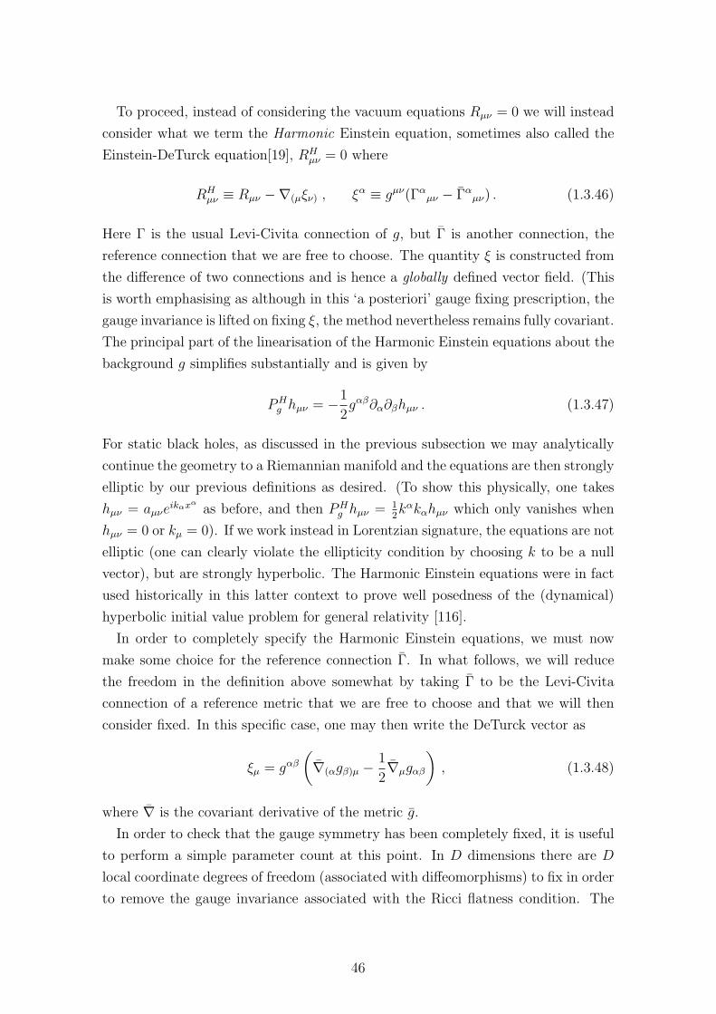
To proceed, instead of considering the vacuum equations Rµν = 0 we will instead

consider what we term the Harmonic Einstein equation, sometimes also called the

Einstein-DeTurck equation[19], RHµν = 0 where

RHµν ≡ Rµν −∇(µξν) , ξα ≡ gµν(Γα

µν − Γαµν) . (1.3.46)

Here Γ is the usual Levi-Civita connection of g, but Γ is another connection, the

reference connection that we are free to choose. The quantity ξ is constructed from

the difference of two connections and is hence a globally defined vector field. (This

is worth emphasising as although in this ‘a posteriori’ gauge fixing prescription, the

gauge invariance is lifted on fixing ξ, the method nevertheless remains fully covariant.

The principal part of the linearisation of the Harmonic Einstein equations about the

background g simplifies substantially and is given by

PHg hµν = −1

2gαβ∂α∂βhµν . (1.3.47)

For static black holes, as discussed in the previous subsection we may analytically

continue the geometry to a Riemannian manifold and the equations are then strongly

elliptic by our previous definitions as desired. (To show this physically, one takes

hµν = aµνeikαxα

as before, and then PHg hµν = 1

2kαkαhµν which only vanishes when

hµν = 0 or kµ = 0). If we work instead in Lorentzian signature, the equations are not

elliptic (one can clearly violate the ellipticity condition by choosing k to be a null

vector), but are strongly hyperbolic. The Harmonic Einstein equations were in fact

used historically in this latter context to prove well posedness of the (dynamical)

hyperbolic initial value problem for general relativity [116].

In order to completely specify the Harmonic Einstein equations, we must now

make some choice for the reference connection Γ. In what follows, we will reduce

the freedom in the definition above somewhat by taking Γ to be the Levi-Civita

connection of a reference metric that we are free to choose and that we will then

consider fixed. In this specific case, one may then write the DeTurck vector as

ξµ = gαβ(

∇(αgβ)µ −1

2∇µgαβ

)

, (1.3.48)

where ∇ is the covariant derivative of the metric g.

In order to check that the gauge symmetry has been completely fixed, it is useful

to perform a simple parameter count at this point. In D dimensions there are D

local coordinate degrees of freedom (associated with diffeomorphisms) to fix in order

to remove the gauge invariance associated with the Ricci flatness condition. The

46

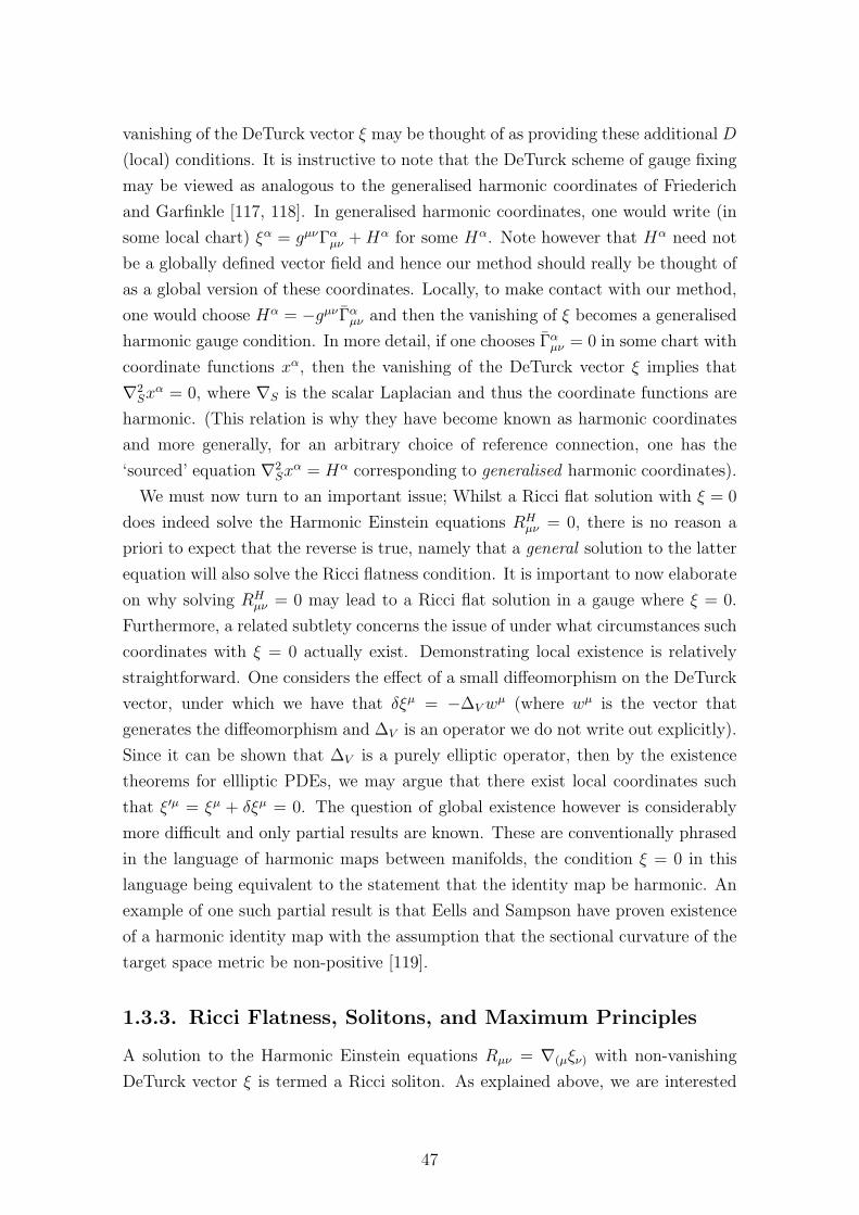
vanishing of the DeTurck vector ξ may be thought of as providing these additional D

(local) conditions. It is instructive to note that the DeTurck scheme of gauge fixing

may be viewed as analogous to the generalised harmonic coordinates of Friederich

and Garfinkle [117, 118]. In generalised harmonic coordinates, one would write (in

some local chart) ξα = gµνΓαµν +Hα for some Hα. Note however that Hα need not

be a globally defined vector field and hence our method should really be thought of

as a global version of these coordinates. Locally, to make contact with our method,

one would choose Hα = −gµνΓαµν and then the vanishing of ξ becomes a generalised

harmonic gauge condition. In more detail, if one chooses Γαµν = 0 in some chart with

coordinate functions xα, then the vanishing of the DeTurck vector ξ implies that

∇2Sx

α = 0, where ∇S is the scalar Laplacian and thus the coordinate functions are

harmonic. (This relation is why they have become known as harmonic coordinates

and more generally, for an arbitrary choice of reference connection, one has the

‘sourced’ equation ∇2Sx

α = Hα corresponding to generalised harmonic coordinates).

We must now turn to an important issue; Whilst a Ricci flat solution with ξ = 0

does indeed solve the Harmonic Einstein equations RHµν = 0, there is no reason a

priori to expect that the reverse is true, namely that a general solution to the latter

equation will also solve the Ricci flatness condition. It is important to now elaborate

on why solving RHµν = 0 may lead to a Ricci flat solution in a gauge where ξ = 0.

Furthermore, a related subtlety concerns the issue of under what circumstances such

coordinates with ξ = 0 actually exist. Demonstrating local existence is relatively

straightforward. One considers the effect of a small diffeomorphism on the DeTurck

vector, under which we have that δξµ = −∆Vwµ (where wµ is the vector that

generates the diffeomorphism and ∆V is an operator we do not write out explicitly).

Since it can be shown that ∆V is a purely elliptic operator, then by the existence

theorems for ellliptic PDEs, we may argue that there exist local coordinates such

that ξ′µ = ξµ + δξµ = 0. The question of global existence however is considerably

more difficult and only partial results are known. These are conventionally phrased

in the language of harmonic maps between manifolds, the condition ξ = 0 in this

language being equivalent to the statement that the identity map be harmonic. An

example of one such partial result is that Eells and Sampson have proven existence

of a harmonic identity map with the assumption that the sectional curvature of the

target space metric be non-positive [119].

1.3.3. Ricci Flatness, Solitons, and Maximum Principles

A solution to the Harmonic Einstein equations Rµν = ∇(µξν) with non-vanishing

DeTurck vector ξ is termed a Ricci soliton. As explained above, we are interested

47

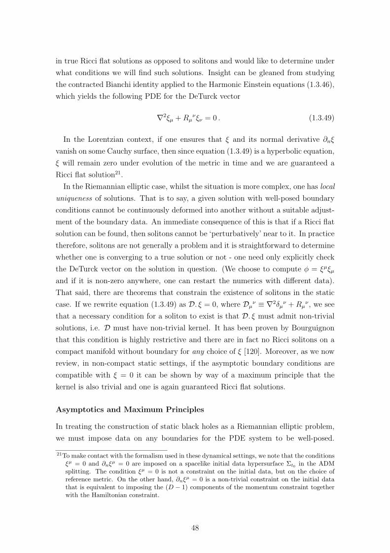
in true Ricci flat solutions as opposed to solitons and would like to determine under

what conditions we will find such solutions. Insight can be gleaned from studying

the contracted Bianchi identity applied to the Harmonic Einstein equations (1.3.46),

which yields the following PDE for the DeTurck vector

∇2ξµ +Rµνξν = 0 . (1.3.49)

In the Lorentzian context, if one ensures that ξ and its normal derivative ∂nξ

vanish on some Cauchy surface, then since equation (1.3.49) is a hyperbolic equation,

ξ will remain zero under evolution of the metric in time and we are guaranteed a

Ricci flat solution21.

In the Riemannian elliptic case, whilst the situation is more complex, one has local

uniqueness of solutions. That is to say, a given solution with well-posed boundary

conditions cannot be continuously deformed into another without a suitable adjust-

ment of the boundary data. An immediate consequence of this is that if a Ricci flat

solution can be found, then solitons cannot be ‘perturbatively’ near to it. In practice

therefore, solitons are not generally a problem and it is straightforward to determine

whether one is converging to a true solution or not - one need only explicitly check

the DeTurck vector on the solution in question. (We choose to compute φ = ξµξµ

and if it is non-zero anywhere, one can restart the numerics with different data).

That said, there are theorems that constrain the existence of solitons in the static

case. If we rewrite equation (1.3.49) as D. ξ = 0, where Dµν ≡ ∇2δµ

ν +Rµν , we see

that a necessary condition for a soliton to exist is that D. ξ must admit non-trivial

solutions, i.e. D must have non-trivial kernel. It has been proven by Bourguignon

that this condition is highly restrictive and there are in fact no Ricci solitons on a

compact manifold without boundary for any choice of ξ [120]. Moreover, as we now

review, in non-compact static settings, if the asymptotic boundary conditions are

compatible with ξ = 0 it can be shown by way of a maximum principle that the

kernel is also trivial and one is again guaranteed Ricci flat solutions.

Asymptotics and Maximum Principles

In treating the construction of static black holes as a Riemannian elliptic problem,

we must impose data on any boundaries for the PDE system to be well-posed.

21To make contact with the formalism used in these dynamical settings, we note that the conditionsξµ = 0 and ∂nξ

µ = 0 are imposed on a spacelike initial data hypersurface Σt0 in the ADMsplitting. The condition ξµ = 0 is not a constraint on the initial data, but on the choice ofreference metric. On the other hand, ∂nξ

µ = 0 is a non-trivial constraint on the initial datathat is equivalent to imposing the (D − 1) components of the momentum constraint togetherwith the Hamiltonian constraint.

48

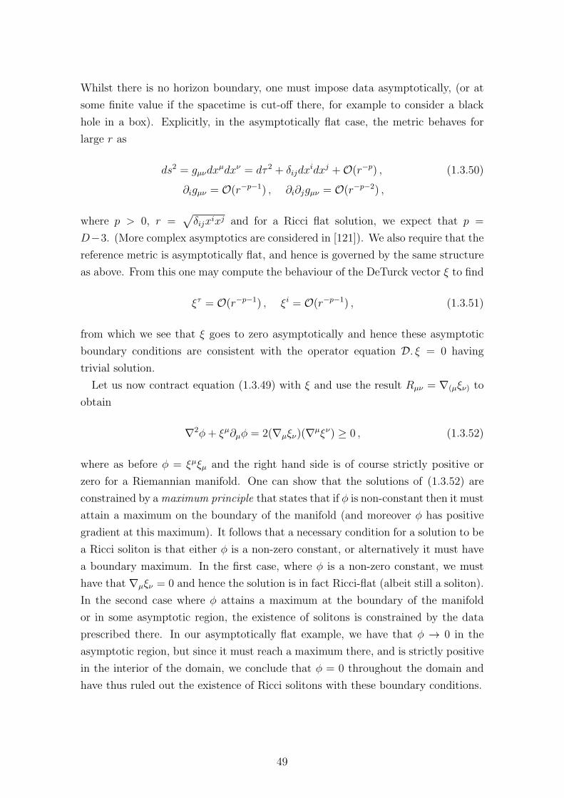
Whilst there is no horizon boundary, one must impose data asymptotically, (or at

some finite value if the spacetime is cut-off there, for example to consider a black

hole in a box). Explicitly, in the asymptotically flat case, the metric behaves for

large r as

ds2 = gµνdxµdxν = dτ 2 + δijdx

idxj +O(r−p) , (1.3.50)

∂igµν = O(r−p−1) , ∂i∂jgµν = O(r−p−2) ,

where p > 0, r =√δijxixj and for a Ricci flat solution, we expect that p =

D−3. (More complex asymptotics are considered in [121]). We also require that the

reference metric is asymptotically flat, and hence is governed by the same structure

as above. From this one may compute the behaviour of the DeTurck vector ξ to find

ξτ = O(r−p−1) , ξi = O(r−p−1) , (1.3.51)

from which we see that ξ goes to zero asymptotically and hence these asymptotic

boundary conditions are consistent with the operator equation D. ξ = 0 having

trivial solution.

Let us now contract equation (1.3.49) with ξ and use the result Rµν = ∇(µξν) to

obtain

∇2φ+ ξµ∂µφ = 2(∇µξν)(∇µξν) ≥ 0 , (1.3.52)

where as before φ = ξµξµ and the right hand side is of course strictly positive or

zero for a Riemannian manifold. One can show that the solutions of (1.3.52) are

constrained by amaximum principle that states that if φ is non-constant then it must

attain a maximum on the boundary of the manifold (and moreover φ has positive

gradient at this maximum). It follows that a necessary condition for a solution to be

a Ricci soliton is that either φ is a non-zero constant, or alternatively it must have

a boundary maximum. In the first case, where φ is a non-zero constant, we must

have that ∇µξν = 0 and hence the solution is in fact Ricci-flat (albeit still a soliton).

In the second case where φ attains a maximum at the boundary of the manifold

or in some asymptotic region, the existence of solitons is constrained by the data

prescribed there. In our asymptotically flat example, we have that φ → 0 in the

asymptotic region, but since it must reach a maximum there, and is strictly positive

in the interior of the domain, we conclude that φ = 0 throughout the domain and

have thus ruled out the existence of Ricci solitons with these boundary conditions.

49

1.3.4. Numerical Implementations

We close this section by outlining some of the methods to numerically solve the

Harmonic Einstein equations. We begin with a treatment of the canonical method

used to solve elliptic systems, namely local relaxation which we will shortly show is

equivalent in our setting to the famous Ricci flow. We then proceed to review the

multidimensional Newton method.

Ricci Flow and Local Relaxation

From the analysis of section (1.3.2), the Harmonic Einstein equations have derivative

structure RHµν = −1

2gαβ∂α∂βgµν +Lµν , where Lµν represent terms with less than two

derivatives. In local relaxation, instead of proceeding to solve the elliptic equations

RHµν = 0 directly, one searches instead for fixed points of the parabolic diffusion

equation

∂gµν(λ)

∂λ= −2RH

µν . (1.3.53)

These equations are then discretised on a lattice of points, and local relaxation is

implemented for example by the standard algorithm due to Jacobi, whereby given

some initial guess for gµν throughout the domain, one iteratively improves the solu-

tion at each point using an update computed from (1.3.53) that depends on nearby

points. (Depending on the order of the differencing, the update can depend on

neighbouring points, next to nearest neighbours etc.).

Regardless of the details of how local relaxation is implemented (Jacobi, Gauss-

Siedel, etc), the continuum diffusion equation that is to be solved is of the form

∂gµν(λ)

∂λ= −2Rµν + 2∇(µξν) , (1.3.54)

which is precisely the Ricci-DeTurck flow, where the second term as discussed previ-

ously corresponds to an infinitesimal diffeomorphism, so that the flow is diffeomor-

phic to the Ricci flow of Hamilton

∂gµν(λ)

∂λ= −2Rµν , (1.3.55)

which has garnered recent fame in pure mathematics for its pivotal role in the

proof of the Poincare conjecture. (An overview of several aspects of Ricci flow

can be found in [122]). We give some initial guess for the parabolic flow and then

run the flow for sufficient time so that we approach the fixed point as closely as

50

desired. Such a point will then satisfy Rµν = 0 as required. An elegant feature

of the Ricci flow picture is that whilst some choice of reference metric is required

to construct the vector ξ that we need to include to make the Einstein DeTurck

equation elliptic (and hence the resulting diffusion equation parabolic), the Ricci-

DeTurck flow is in fact diffeomorphic to pure Ricci flow which makes no mention

of ξ and therefore the reference metric. What this means is that given some initial

guess metric, whilst different choices of reference will change the path taken by the

flow in the space of metrics, it will not change the path in the space of physical

geometries (i.e. metrics modulo diffeomorphisms) - this path is always the same.

Moreover, provided one chooses a reference metric that shares the same isometries

as the ‘physical’ spacetime metric, then the Harmonic Einstein tensor will also be

symmetric under these isometries and furthermore these isometries will be preserved

under the flow.

It is instructive to study Ricci flow itself a little further. Physically it can be

thought of as a diffusion equation for geometry that locally tries to smooth out

curvature. Suppose we have some Ricci flat solution gµν and wish to consider the

Ricci flow of a perturbation hµν to this. From (1.3.43) we have

∂hµν∂λ

= −2∆Lhµν − 2∇(µνν) , (1.3.56)

where the last term is an infinitesimal diffeomorphism generated by v. For Euclidean

space, this flow is then diffeomorphic to a flow where each component of the metric

diffuses as, ∂hµν

∂λ= δαβ∂α∂βhµν and hence we conclude that Euclidean space is stable

to linear perturbations. The flow however has many additional striking non-linear

features that cannot easily be seen at this perturbative level. For example, it col-

lapses regions of positive curvature, a fact that can seen by studying the Ricci flow

of the round sphere whose radius shrinks with time, eventually collapsing to zero

radius in finite time. A further important property of Ricci flow is that it can be

shown to preserve asymptotic flatness for short times [123].

It is important to note that a Ricci flat solution will only be stable to perturbations

if the Lichnerowicz operator is positive (has positive eigenvalue spectrum). Whilst

one is justified in assuming the absence of zero modes, as these can be removed

by specification of appropriate boundary data, it is unclear that ∆L must have a

positive spectrum and indeed in a variety of scenarios it does not, so that there exist

eigenfunctions with negative eigenvalue. When perturbed by these, such eigenmodes

grow exponentially so that at late times the perturbation will flow away from the

fixed point in these directions, perhaps ending at some other fixed point. Indeed

51

a fundamental property of static black holes is that the positivity of ∆L on these

backgrounds is tied to their thermodynamics22 (since the Euclidean action is simply

related to the free energy [56]) and many simple examples of interest possess negative

modes. A classic example is the Euclidean Schwarzchild black hole which has a

single negative mode discovered by Gross, Perry and Yaffe [128]. Negative modes

can present a problem for numerics as one has to fine tune initial data in order

to hit a solution. We will not review this procedure here, but refer the reader

to the literature [21]. Due to the difficulties associated with negative modes, all

subsequent elliptic numerics in this thesis will make use of a different numerical

algorithm to solve such systems namely Newton’s method, a subject to which we

now turn. It is worth emphasising beforehand though that despite its difficulties,

local relaxation remains in many ways simpler and more elegant than Newton’s

method and moreover, there are physically relevant situations that are stable under

Ricci flow where these techniques are directly useful, a prime example being to find

solutions in AdS/CFT where the boundary metric is a black hole [121].

Newton’s Method

As we have just seen, whilst local relaxation is elegant and simple to implement it

suffers the problem of sensitivity to negative modes and becomes ill suited to use in

many practical situations. Fortunately, there is another standard technique to solve

elliptic systems known as Newton’s method that is insensitive to the stability of the

fixed points. Unfortunately it is somewhat more technical to implement than local

relaxation and is arguable less elegant (in that it doesn’t share the beautiful global

geometric features of Ricci flow, such as independence of the background metric). In

addition, the basin of attraction for the Newton method is generically rather small

(and background dependent), so choosing an initial guess can be something of a

challenge. The optimal approach is in fact probably to start with some initial guess,

and then use Ricci flow (which doesn’t need to start within a basin of attraction)

to relax close enough to a solution and then switch to the Newton method (before

the negative mode becomes an issue) when one is within the basin of attraction of

the fixed point. We should then converge very rapidly to a solution.

22Gubser and Mitra conjectured a link between classical and thermodynamic instabilities of hori-zons [124, 125]. They argued that there is a gravitational instability of a black brane preciselyif the horizon has a thermodynamic instability (i.e. negative specific heat). The argument pro-ceeds by using Euclidean quantum gravity to calculate the free energy from the gravitationalaction and then proves that solutions have Euclidean negative modes if they have negative spe-cific heat (see [126] for a clear account of this and moreover a discussion of when the conversealso holds). Many assumptions are made in these analyses and it has now been demonstratedthat there are counterexamples to the general conjecture [127].

52

To implement the Newton method, we again imagine discretising our system on a

lattice. If we perturb the metric g as g+ ǫδg, the Harmonic Einstein tensor changes

as

RHM(g + ǫδg) = RH

M(g) + ǫ O(g)MNδgN +O(ǫ2) , (1.3.57)

where the matrix O(g)NM is the linearisation of the Harmonic Einstein tensor RHM .

If we begin with some initial guess metric g(A)M , then Newton’s method iteratively

improves this guess as

g(A+1)M = g

(A)M − (O(g(A))−1)M

NRHN (g

(A)) . (1.3.58)

As with the well-known one dimensional version, this method moves along the tan-

gent to the equations to find a solution and will converge very quickly when it is

near a fixed point. As with Ricci flow, provided the reference metric is chosen to

share the same isometries as the physical metric, then the Harmonic Einstein tensor

will be symmetric under these and the Newton method will preserve this structure.

In summary, the Newton method has the very important advantage over the Ricci-

DeTurck flow that it is not sensitive to negative modes and this makes it much more

practically useful than local relaxation, provided one can construct a suitable initial

guess. The payoff is that its numerical implementation is somewhat non-trivial and

in particular it assumes that the linear problem O.V = RH can be solved for the

vector V . In settings where a ‘good’ initial guess can be physically motivated, the

Newton method is very powerful - we shall see this in detail when we use it to

construct static and stationary black holes in a modified theory of gravity known

as Einstein Aether theory in chapter (4). There we will see that we have analytic

forms for the initial guess that are expected to be close to the new solutions and the

Newton method then rapidly converges to the desired fixed points.

1.4. Einstein-Aether Gravity

In recent years there has been considerable interest in the possibility that Lorentz

invariance is violated by quantum gravity effects. Indeed, such Lorentz violating

processes underpin much of the current phenomenology of theories such as loop

quantum gravity as well as certain aspects of string theory (see for example [129, 130,

131, 132]). Whilst in the context of particle physics, Lorentz violation in the matter

sector, captured within the framework of the Standard Model Extension (SME)

[133] is highly constrained, in gravitational settings the situation is far less restricted

53

[134, 135]. One can break Lorentz symmetry by the inclusion of fixed background

fields but this is not an option in the presence of gravity as if we are to preserve

the precise experimental successes of pure general relativity, we had better maintain

general covariance. One option is to promote the Lorentz violating background fields

to dynamical fields that are governed by a generally covariant action and in this

chapter we will discuss a model example of Lorentz violation in the gravitational

sector known as Einstein-Aether theory which does just this. In particular, this

theory spontaneously breaks Lorentz symmetry and has the property that every

field configuration one might imagine breaks Lorentz symmetry everywhere, even

in the ‘vacuum’. (Of course, almost any gravitational solution in general relativity

breaks Lorentz symmetry but what one has in mind with Einstein-Aether theory

is something stronger than that. In detail, whilst a solution in general relativity

might break Lorentz symmetry, it must ultimately be restored on small scales, as

the geometry locally looks like Minkowski space. In Einstein-Aether theory however,

this is no longer true as Lorentz symmetry is broken even on small scales by the

aether field that we introduce shortly).

If Lorentz violation is to preserve isotropy at every point (three dimensional rota-

tions), then the associated background field (that breaks Lorentz symmetry) must

be described by a timelike vector at each point in spacetime. In Einstein-Aether

theory this is described by a vector field uµ which should be thought of as the mini-

mal structure one must impose to be able to determine a locally preferred rest frame

[22, 23, 136, 137]. This vector field uµ known as the aether is ubiquitous throughout

spacetime and is named after the famed lumeniferous aether of turn of the century

physics23.

We are ultimately interested in applying our numerical techniques (with some

modifications) to construct black holes in Einstein-Aether theory, a subject we will

turn to in chapter 4. This section serves as an introduction to the theory. We

present the action and field equations of Einstein-Aether in various forms and then

discuss the various field redefinitions one can use to somewhat simplify the highly

complex field equations. We then investigate the propagating degrees of freedom

contained in the theory, demonstrating that there are a total of five modes - the

23There has also been more recent work on ‘aether theories’, notably the vector-tensor theories ofthe 1970s [138, 139, 140]. These differ from the version we present in this thesis in that we willrequire our aether field to be normalised. Early work has also been done by Gasperini in thiscontext using the tetrad formalism [136]. In cosmology, vector-tensor theories have been studiedby Clayton and Moffatt [141, 142] as well as Bassett et al [143] and shocks have been studiedby Clayton [144]. More recently, Arkani-Hamed et al [145, 146] have proposed a string-inspiredmechanism for Lorentz symmetry breaking in a similar ‘spirit’ to Einstein-Aether (whereby thegradient of a scalar is fixed to be of constant norm) and finally we note also the systematicanalysis of Lorentz violation in general gravitational settings of Kostelecky [147].

54

two gravitational waves of general relativity, together with a further three coupled

aether-metric modes. We close with a brief discussion of the current experimental

bounds on the theory that come from a variety of sources including post-Newtonian

analysis and cosmology.

1.4.1. Action and Field Equations

Einstein-Aether theory is a diffeomorphism invariant model for Lorentz violation in

the gravitational sector. In this theory, Lorentz symmetry is spontaneously broken

by the inclusion of a dynamical vector field known as the aether uµ(x). This aether

field acquires a unit timelike vacuum expectation value (VEV) that is enforced

dynamically at the level of the action through a Lagrange multiplier constraint (for

a review, see [24]). Whilst the field content of the theory is simply gravity and a

vector field (not a gauge field), as we shall discuss, the broken Lorentz symmetry

leads to a complex spectrum of propagating degrees of freedom and an intricate

causal structure governed by multiple ‘light’ cones (and hence effective metrics). As

one might expect, this makes the nature of its black hole solutions rather different

from in general relativity.

In much of the literature on Einstein-Aether theory, the authors discuss the theory

in mostly minus (+,−,−,−) signature. In this thesis, we will however use the mostly

plus (−,+,+,+) signature, in which the action (in the absence of matter) takes the

form

S =1

16πG

∫

d4x√−g

[R−Kµν

αβ (∇µuα)(∇νu

β)+ λ(gµνu

µuν + 1)], (1.4.59)

where R is the Ricci scalar, G is the gravitational coupling constant (that is generi-

cally different from the Newton constant GN in pure general relativity as the terms

quadratic in the gradient of the aether field ∇u change the kinetic terms for the

metric). The tensor Kµναβ is defined as

Kµναβ := c1g

µνgαβ + c2δµαδ

νβ + c3δ

µβδ

να − c4u

µuνgαβ , (1.4.60)

where the ci (i = 1, 2, 3, 4) are dimensionless arbitrary coupling constants, and the

term proportional to the Lagrange multiplier λ enforces the constraint that the

aether field lie on the unit hyperboloid. It is this Lagrange multiplier together with

the c4 term that distinguishes the theory from the vector tensor theories of [148].

The tensor Kµναβ should be thought as the most general polynomial in u that is

irreducible under the constraint, in the sense that it contains no u terms that can

55

be covariantly reduced by imposing the constraint equation. (One example of a

reducible object would be a term that is proportional to uµ∇σuµ). Moreover, terms

of the form Rabuaub are also not included as these are proportional to the difference

between the c2 and c3 terms by integration by parts. It will be convenient in what

follows to introduce the quantity

Jµν ≡ Kµανβ∇αuβ = c1∇µuν + c2gµν∇.u+ c3∇νuµ − c4u

µuν , (1.4.61)

where we note that Jµν is not symmetric in its indices. The action may then be

written more succinctly as

S =1

16πG

∫

d4x√−g

(R− Jµν∇µuν + λ(u2 + 1)

). (1.4.62)

The field equations are obtained by varying the action and one finds that

Gµν = − ∇α

[Jα

(µuν) + J(µαuν) − J(µν)u

α]− 1

2gµνJ

αβ∇αuβ

+ c1[(∇(µu

α)∇ν)uα + (∇αu(µ)∇αuν)]

+ 2c2(∇.u)∇(µuν)

+ c3[(∇(µu

α)∇|α|uν) + (∇αu(µ)∇ν)uα]

− c4[2aαu(µ∇ν)u

α + aµaν]

− λ

(

uµuν −1

2gµν(u

2 + 1)

)

, (1.4.63)

where Gµν = Rµν − 12gµνR is the Einstein tensor, J = Jµ

µ and we have defined the

‘acceleration’ aµ = uα∇αuµ . For the vector equation we have

∇αJαµ + c4aα∇µuα + λuµ = 0 , (1.4.64)

and finally the scalar (constraint) equation is

gµνuµuν + 1 = 0 . (1.4.65)

In view of the fact that we will later be interested in solving the Harmonic Ein-

stein equation in order to find black hole solutions, it will be useful to rewrite the

56

gravitational equations in terms of the Ricci tensor

Rµν = − ∇α

[Jα

(µuν) + J(µαuν) − J(µν)u

α]

+1

2gµν∇α

[(Jαβ + Jβα)uβ − Juα

]+

1

2gµνJ

αβ∇αuβ

+ c1[(∇(µu

α)∇ν)uα + (∇αu(µ)∇αuν) − gµν(∇αuβ)(∇αuβ)]

+ c2(∇.u)[2∇(µuν) − gµν(∇.u)

]

+ c3[(∇(µu

α)∇|α|uν) + (∇αu(µ)∇ν)uα − gµν(∇αuβ)(∇βuα)]

− c4

[

2aαu(µ∇ν)uα + aµaν −

3

2gµνa

2

]

− λ

(

uµuν +1

2gµν

)

. (1.4.66)

The equations ((1.4.63), (1.4.66)) are what one finds on directly varying the action,

and we will use this form (when supplemented by a DeTurck term) in our later

calculations. We note for completeness however that the equations of Einstein-

Aether theory are often presented in a somewhat different way in the literature (see

for example [149, 150]). One can arrive at this alternate (and simplified) form by

directly substituting the aether and scalar equations into (1.4.63), to arrive at

Gµν = ∇α

[J(µν)u

α + Jα(µuν) − J(µ

αuν)]− 1

2gµνJ

αβ(∇αuβ)

+ c1[(∇(µu

α)(∇ν)uα)− (∇αu(µ)(∇αuν))]+ c4aµaν

+ λuµuν , (1.4.67)

or equivalently

Rµν = ∇α

[J(µν)u

α + Jα(µuν) − J(µ

αuν)]

− 1

2gµν∇α

[J (β

β)uα + Jα(βuβ) − J (β|α|uβ)

]+

1

2gµνJ

αβ(∇αuβ)

+ c1[(∇(µu

α)(∇ν)uα)− (∇αu(µ)(∇αuν))]

+ c4

[

aµaν −1

2gµνa

2

]

+ λ

(

uµuν +1

2gµν

)

. (1.4.68)

One may further eliminate the Lagrange multiplier λ if desired from these equations

by considering the trace of the aether equation (1.4.64) which reveals that

λ = c4(aαaα) + (∇αJ

αβ)u

β . (1.4.69)

57

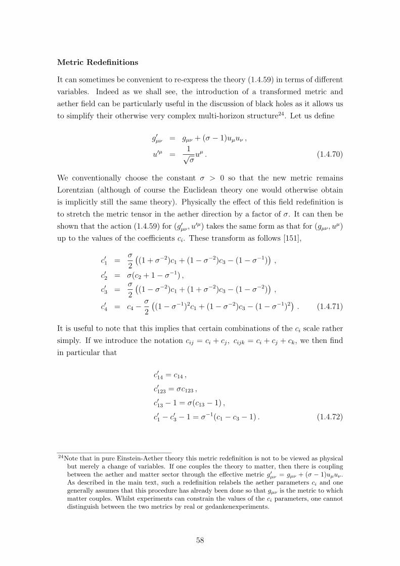
Metric Redefinitions

It can sometimes be convenient to re-express the theory (1.4.59) in terms of different

variables. Indeed as we shall see, the introduction of a transformed metric and

aether field can be particularly useful in the discussion of black holes as it allows us

to simplify their otherwise very complex multi-horizon structure24. Let us define

g′µν = gµν + (σ − 1)uµuν ,

u′µ =1√σuµ . (1.4.70)

We conventionally choose the constant σ > 0 so that the new metric remains

Lorentzian (although of course the Euclidean theory one would otherwise obtain

is implicitly still the same theory). Physically the effect of this field redefinition is

to stretch the metric tensor in the aether direction by a factor of σ. It can then be

shown that the action (1.4.59) for (g′µν , u′µ) takes the same form as that for (gµν , u

µ)

up to the values of the coefficients ci. These transform as follows [151],

c′1 =σ

2

((1 + σ−2)c1 + (1− σ−2)c3 − (1− σ−1)

),

c′2 = σ(c2 + 1− σ−1) ,

c′3 =σ

2

((1− σ−2)c1 + (1 + σ−2)c3 − (1− σ−2)

),

c′4 = c4 −σ

2

((1− σ−1)2c1 + (1− σ−2)c3 − (1− σ−1)2

). (1.4.71)

It is useful to note that this implies that certain combinations of the ci scale rather

simply. If we introduce the notation cij = ci + cj, cijk = ci + cj + ck, we then find

in particular that

c′14 = c14 ,

c′123 = σc123 ,

c′13 − 1 = σ(c13 − 1) ,

c′1 − c′3 − 1 = σ−1(c1 − c3 − 1) . (1.4.72)

24Note that in pure Einstein-Aether theory this metric redefinition is not to be viewed as physicalbut merely a change of variables. If one couples the theory to matter, then there is couplingbetween the aether and matter sector through the effective metric g′µν = gµν + (σ − 1)uµuν .As described in the main text, such a redefinition relabels the aether parameters ci and onegenerally assumes that this procedure has already been done so that gµν is the metric to whichmatter couples. Whilst experiments can constrain the values of the ci parameters, one cannotdistinguish between the two metrics by real or gedankenexperiments.

58

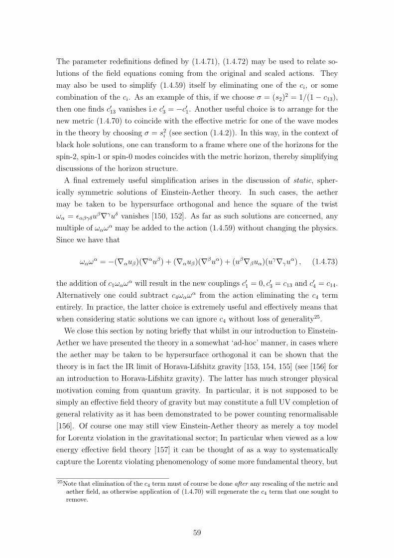
The parameter redefinitions defined by (1.4.71), (1.4.72) may be used to relate so-

lutions of the field equations coming from the original and scaled actions. They

may also be used to simplify (1.4.59) itself by eliminating one of the ci, or some

combination of the ci. As an example of this, if we choose σ = (s2)2 = 1/(1− c13),

then one finds c′13 vanishes i.e c′3 = −c′1. Another useful choice is to arrange for the

new metric (1.4.70) to coincide with the effective metric for one of the wave modes

in the theory by choosing σ = s2i (see section (1.4.2)). In this way, in the context of

black hole solutions, one can transform to a frame where one of the horizons for the

spin-2, spin-1 or spin-0 modes coincides with the metric horizon, thereby simplifying

discussions of the horizon structure.

A final extremely useful simplification arises in the discussion of static, spher-

ically symmetric solutions of Einstein-Aether theory. In such cases, the aether

may be taken to be hypersurface orthogonal and hence the square of the twist

ωα = ǫαβγδuβ∇γuδ vanishes [150, 152]. As far as such solutions are concerned, any

multiple of ωαωα may be added to the action (1.4.59) without changing the physics.

Since we have that

ωαωα = −(∇αuβ)(∇αuβ) + (∇αuβ)(∇βuα) + (uβ∇βuα)(u

γ∇γuα) , (1.4.73)

the addition of c1ωαωα will result in the new couplings c′1 = 0, c′3 = c13 and c

′4 = c14.

Alternatively one could subtract c4ωαωα from the action eliminating the c4 term

entirely. In practice, the latter choice is extremely useful and effectively means that

when considering static solutions we can ignore c4 without loss of generality25.

We close this section by noting briefly that whilst in our introduction to Einstein-

Aether we have presented the theory in a somewhat ‘ad-hoc’ manner, in cases where

the aether may be taken to be hypersurface orthogonal it can be shown that the

theory is in fact the IR limit of Horava-Lifshitz gravity [153, 154, 155] (see [156] for

an introduction to Horava-Lifshitz gravity). The latter has much stronger physical

motivation coming from quantum gravity. In particular, it is not supposed to be

simply an effective field theory of gravity but may constitute a full UV completion of

general relativity as it has been demonstrated to be power counting renormalisable

[156]. Of course one may still view Einstein-Aether theory as merely a toy model

for Lorentz violation in the gravitational sector; In particular when viewed as a low

energy effective field theory [157] it can be thought of as a way to systematically

capture the Lorentz violating phenomenology of some more fundamental theory, but

25Note that elimination of the c4 term must of course be done after any rescaling of the metric andaether field, as otherwise application of (1.4.70) will regenerate the c4 term that one sought toremove.

59

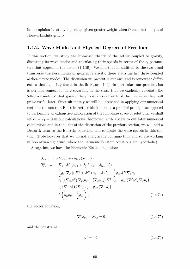
in our opinion its study is perhaps given greater weight when framed in the light of

Horava-Lifshitz gravity.

1.4.2. Wave Modes and Physical Degrees of Freedom

In this section, we study the linearised theory of the aether coupled to gravity,

discussing its wave modes and calculating their speeds in terms of the ci parame-

ters that appear in the action (1.4.59). We find that in addition to the two usual

transverse traceless modes of general relativity, there are a further three coupled

aether-metric modes. The discussion we present is our own and is somewhat differ-

ent to that explicitly found in the literature [149]. In particular, our presentation

is perhaps somewhat more covariant in the sense that we explicitly calculate the

‘effective metrics’ that govern the propagation of each of the modes as they will

prove useful later. Since ultimately we will be interested in applying our numerical

methods to construct Einstein-Aether black holes as a proof of principle as opposed

to performing an exhaustive exploration of the full phase space of solutions, we shall

set c3 = c4 = 0 in our calculations. Moreover, with a view to our later numerical

calculations and in the light of the discussion of the previous section, we will add a

DeTurck term to the Einstein equations and compute the wave speeds in this set-

ting. (Note however that we do not analytically continue time and so are working

in Lorentzian signature, where the harmonic Einstein equations are hyperbolic).

Altogether, we have the Harmonic Einstein equation:

Jµν = c1∇µuν + c2gµν (∇ · u) ,RH

µν = −∇σ

(Jσ

(µuν) + J σ(µ uν) − J(µν)u

σ)

+1

2gµν∇σ ((J

σρ + Jρσ) uρ − Juσ) +1

2gµνJ

σρ∇σuρ

+c1((∇(µu

σ)∇ν)uσ +

(∇σu(µ

)∇σuν) − gµν (∇σuρ)∇σuρ

)

+c2 (∇ · u)(2∇(µuν) − gµν (∇ · u)

)

+λ

(

uµuν +1

2gµν

)

, (1.4.74)

the vector equation,

∇σJσµ + λuµ = 0 , (1.4.75)

and the constraint,

u2 = −1 , (1.4.76)

60

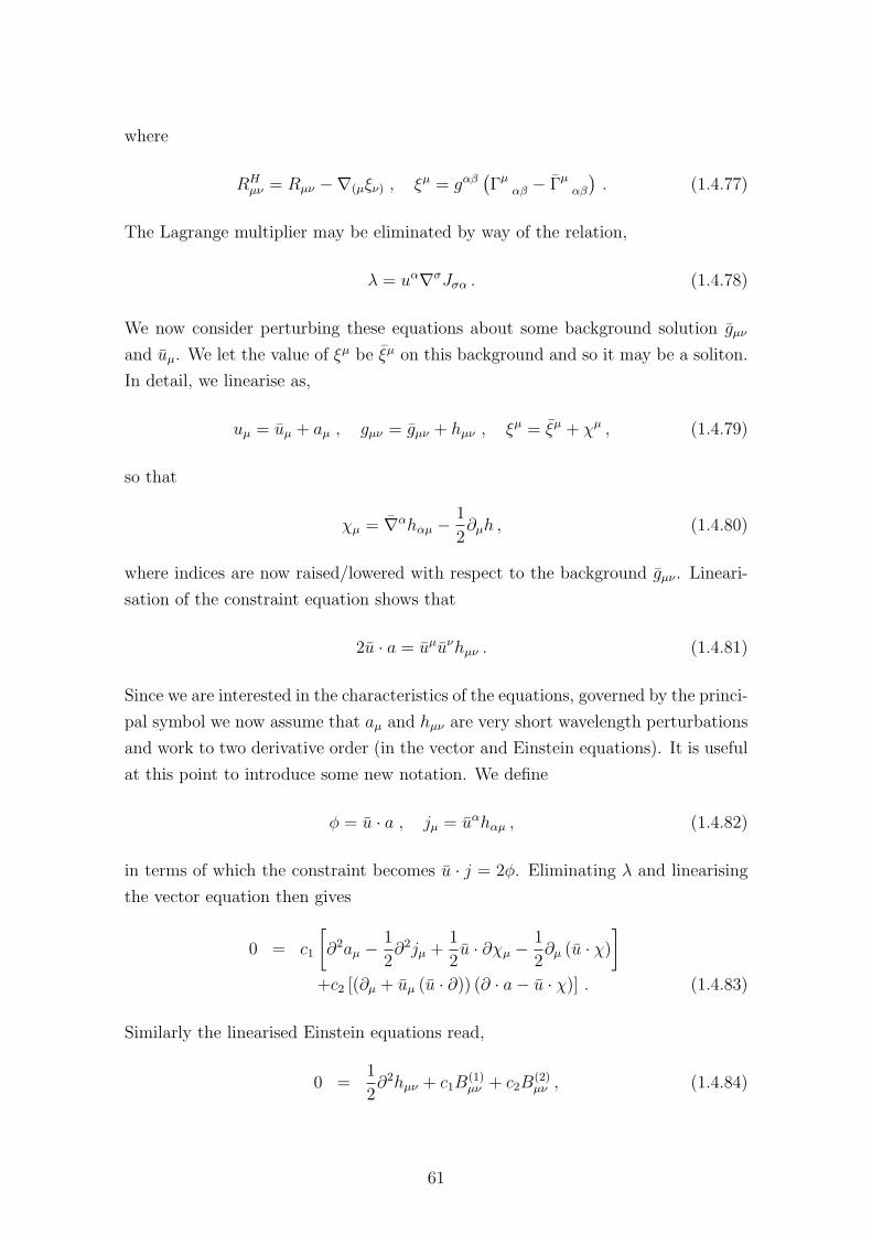
where

RHµν = Rµν −∇(µξν) , ξµ = gαβ

(Γµ

αβ − Γµαβ

). (1.4.77)

The Lagrange multiplier may be eliminated by way of the relation,

λ = uα∇σJσα . (1.4.78)

We now consider perturbing these equations about some background solution gµν

and uµ. We let the value of ξµ be ξµ on this background and so it may be a soliton.

In detail, we linearise as,

uµ = uµ + aµ , gµν = gµν + hµν , ξµ = ξµ + χµ , (1.4.79)

so that

χµ = ∇αhαµ −1

2∂µh , (1.4.80)

where indices are now raised/lowered with respect to the background gµν . Lineari-

sation of the constraint equation shows that

2u · a = uµuνhµν . (1.4.81)

Since we are interested in the characteristics of the equations, governed by the princi-

pal symbol we now assume that aµ and hµν are very short wavelength perturbations

and work to two derivative order (in the vector and Einstein equations). It is useful

at this point to introduce some new notation. We define

φ = u · a , jµ = uαhαµ , (1.4.82)

in terms of which the constraint becomes u · j = 2φ. Eliminating λ and linearising

the vector equation then gives

0 = c1

[

∂2aµ −1

2∂2jµ +

1

2u · ∂χµ −

1

2∂µ (u · χ)

]

+c2 [(∂µ + uµ (u · ∂)) (∂ · a− u · χ)] . (1.4.83)

Similarly the linearised Einstein equations read,

0 =1

2∂2hµν + c1B

(1)µν + c2B

(2)µν , (1.4.84)

61

with

B(1)µν =

(1

2(u · ∂)2 hµν + (u · ∂)

(∂(µaν) − ∂(µjν)

))

+ u(µ(∂2jν − ∂2aν − (u · ∂) ξν)

)

−u(µ∂ν) (∂ · a− u · χ)− 1

2gµν(∂2φ− (u · ∂) (u · χ)

),

B(2)µν = −2u(µ∂ν) (∂ · a− u · χ)−

(

uµuν +1

2gµν

)

(u · ∂) (∂ · a− u · χ) . (1.4.85)

To derive the wave modes, it is useful at this point to contract the Einstein equations

(1.4.84) with uµ and combine this with the vector equation (1.4.83) to eliminate jµ.

Following this prescription, one obtains a second vector equation

0 = c1 (2− c1)(∂2aµ − ∂µ (u · χ)

)+(2c2 − 3c1c2 − c21

)uµ (u · ∂) (∂ · a− u · χ)

+(2c2 + c21

)∂µ (∂ · a− u · χ) + c21

((u · ∂)2 aµ − (u · ∂) ∂µφ

)

+c1(∂µ(u.χ) + u.∂χµ) . (1.4.86)

One may explicitly check that Sµν = c1B(1)µν + c2B

(2)µν is conserved

∂αSαµ −1

2∂µS = 0 , (1.4.87)

and since the Einstein equations are

∂2hµν = −2Sµν , (1.4.88)

this implies that

0 = ∂2(

∂αhαµ −1

2∂µh

)

= ∂2χµ . (1.4.89)

This equation has a very important consequence that simplifies calculations consid-

erably. As we shall discuss shortly, the various perturbation modes in the theory

obey wave equations of the form

(∂2 + q (u · ∂)2

)Φµ... = 0 , (1.4.90)

for constants q that depend on the spin of the perturbation Φµ... and translate into

a wave speed s according to

s2 =1

1− q, (1.4.91)

62

where s = 1 is the speed of light. Equation (1.4.89) implies that only for perturba-

tions with q = 0, (so s = 1), such that ∂2 annihilates the perturbation can we have a

non-vanishing χµ26. As we now demonstrate, the physical spin-2, spin-1 and spin-0

perturbations generically all have q 6= 0 (unless one chooses specific ci parameters)

and hence must all have vanishing χµ. In fact only the gauge perturbations have

q = 0 and in this case one may explicitly calculate that χµ = 0 as well so that

then all modes satisfy this condition. We may now proceed to study the different

perturbations in some detail, beginning with gauge modes.

Gauge Transformations:

A gauge transformation is given by a perturbation of the form,

hµν = ∂µvν + ∂νvµ , aµ = ∂µ (u · v) , (1.4.92)

where vµ generates the diffeomorphism, and χµ = ∂2vµ for this perturbation.

One may show by direct calculation that the vector equation (1.4.83) vanishes

on gauge transformations as it is composed solely of gauge invariant terms (such as

∂ · a − u · χ). Similarly, B(1)µν and B

(2)µν are gauge invariant as well. The Harmonic

Einstein tensor on such a perturbation therefore yields

∂2(∂(µvν)

)= 0 , (1.4.93)

where this derivative structure arises as a consequence of the DeTurck term (recall

(1.3.47)). We see from this that gauge perturbations acquire a kinetic term and

obey a wave equation that is governed by the metric gαβ. Note also that the gauge

modes have q = 0 in the notation of equation (1.4.90). Finally, since we have that

χµ = ∂2vµ, we may conclude that χµ = 0 and so the latter is unperturbed. (Once

again to see this, expand the perturbation χµ in harmonics).

Physical Degrees of Freedom

We now consider the propagating spin-2, spin-1 and spin-0 degrees of freedom in the

theory. To proceed, we may set χµ = 0 (preempting the fact that these modes will

all have q = 0) and consider two further contractions of the vector equation 1.4.86.

26To see this explicitly, expand the perturbations in a plane wave basis χµ =∑

a α(a)µ eik

(a).x,

Φµν... =∑

a φ(a)µν...eik

(a).x and substitute into (1.4.89), (1.4.90). We see from (1.4.90) that whenq 6= 0, we must have k 6= 0 and (1.4.89) then implies that αµ = 0 =⇒ χµ = 0.

63

❼ Spin-0

We may contract with ∂µ and uµ to obtain,

0 = 2 (c1 + c2) ∂2 (∂ · a) + (2c2 − 3c1c2) (u · ∂)2 (∂ · a)− c21 (u · ∂) ∂2φ ,

0 = (2− c1) ∂2φ+ (2c1 + 3c2) (u · ∂) (∂ · a) (1.4.94)

respectively. Eliminating ∂2φ between these equations we then obtain

(∂2 + q(0) (u · ∂)2

)(∂ · a) = 0 , q(0) =

c31 + 2c2 − 4c1c2 + 3c21c2(c1 + c2) (2− c1)

. (1.4.95)

We see from this that the degree of freedom ∂.a propagates with speed s2(0) =

1/(1− q(0)). It is the spin-0 degree of freedom.

❼ Spin-2

If we now consider a perturbation with aµ = 0 (and hence φ = 0) we see that

it automatically satisfies the vector equation (1.4.86). The Einstein equation

(1.4.84) for such a mode becomes

−1

2

(∂2 + q(2) (u · ∂)2

)hµν = 0 , q(2) = c1 . (1.4.96)

We therefore see that this is a mode with q(2) = c1 and speed s2(2) = 1/(1− c1).Note that when c1 = 0, this mode propagates at the speed of light and hence

corresponds to the usual spin-2 degree of freedom in general relativity.

❼ Spin-1

Finally we discuss vector perturbations where ∂.a = 0. Note that if this

quantity does not vanish, the wave speed of such a perturbation would of

course be constrained to propagate with speed q(0) as in (1.4.95), but in the

vanishing case, the wave speed may be different. Note also that provided

q 6= 0, then φ = 0. We consider a mode of the form,

aµ = nµ , u · n = ∂ · n = 0 , χµ = 0 , (1.4.97)

64

where nµ has two polarization states after the constraints u · a = 0 and φ =

∂ · a = 0 are imposed. The vector equation (1.4.86) then implies

0 = c1 (2− c1) ∂2nµ + c21 (u · ∂)2 nµ , (1.4.98)

so that

0 =(∂2 + q(1) (u · ∂)2

)nµ , q(1) =

c12− c1

. (1.4.99)

These are the two spin-1 vector modes.

In summary, we have displayed the five physical degrees of freedom that are

present in Einstein-Aether theory. Our choice of DeTurck term results in the gauge

modes acquiring a kinetic term governed solely by the metric gαβ, in other words

q(gauge) = 0. All the physical perturbations on the other hand are governed by

effective metrics of the form (gµν + q(physical)uµuν) with q(physical) 6= 0 (generically),

so that χµ = 0. Recalling the definition of the perturbation χµ, this essentially

means that they are in Lorentz gauge. We close by noting that this behaviour is

of course related to our choice of DeTurck term. One could envision choosing a

‘modified’ DeTurck term involving the aether

RHµν = Rµν −∇(µξν) + k1 (u · ∂)

(u(µξν)

)+ k2u(µ∂ν) (u · ξ) + (k3gµν + k4uµuν) (∂ · ξ) ,

for some constants k1, k2, k3, k4 in the hopes that the equations of motion might sim-

plify further. The difficulty with this however is that the effective metric governing

the gauge fluctuations would no longer simply be gµν and thus it becomes difficult

to distinguish gauge fluctuations from physical modes. Indeed, the two may mix in

this case whilst with our choice of DeTurck term, there is no such mixing and it is

straightforward to distinguish the two.

1.4.3. Constraints on the Parameter Space

To close our introduction to Einstein-Aether theory, we briefly review for complete-

ness some of the experimental and theoretical constraints on the parameters ci.

Whilst for the purposes of this thesis, we have not always restricted the black hole

solutions we construct in chapter 4 to lie in phenomenologically allowed regions of

parameter space, in our forthcoming paper it would be interesting to do so.

65

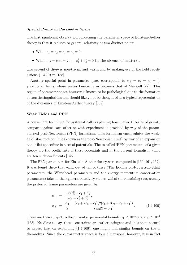
Special Points in Parameter Space

The first significant observation concerning the parameter space of Einstein-Aether

theory is that it reduces to general relativity at two distinct points,

❼ When c1 = c2 = c3 = c4 = 0 .

❼ When c14 = c123 = 2c1 − c21 + c23 = 0 (in the absence of matter) .

The second of these is non-trivial and was found by making use of the field redefi-

nitions (1.4.70) in [158].

Another special point in parameter space corresponds to c13 = c2 = c4 = 0,

yielding a theory whose vector kinetic term becomes that of Maxwell [22]. This

region of parameter space however is known to be pathological due to the formation

of caustic singularities and should likely not be thought of as a typical representation

of the dynamics of Einstein Aether theory [159].

Weak Fields and PPN

A convenient technique for systematically capturing how metric theories of gravity

compare against each other or with experiment is provided by way of the param-

eterised post-Newtonian (PPN) formalism. This formalism encapsulates the weak-

field, slow motion limit (known as the post-Newtonian limit) by way of an expansion

about flat spacetime in a set of potentials. The so called ‘PPN parameters’ of a given

theory are the coefficients of these potentials and in the current formalism, there

are ten such coefficients [148].

The PPN parameters for Einstein-Aether theory were computed in [160, 161, 162].

It was found there that eight out of ten of these (The Eddington-Robertson-Schiff

parameters, the Whitehead parameters and the energy momentum conservation

parameters) take on their general relativity values, whilst the remaining two, namely

the preferred frame parameters are given by,

α1 =−8(c23 + c1 + c42c1 − c21 + c23

,

α2 =α1

2− (c1 + 2c3 − c4)(2(c1 + 3c2 + c3 + c4))

c123(2− c14). (1.4.100)

These are then subject to the current experimental bounds α1 < 10−4 and α2 < 10−7

[163]. Needless to say, these constraints are rather stringent and it is then natural

to expect that on expanding (1.4.100), one might find similar bounds on the ci

themselves. Since the ci parameter space is four dimensional however, it is in fact

66

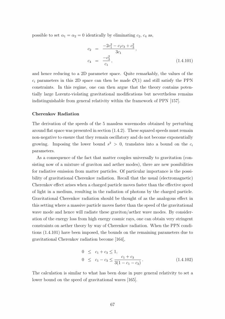
possible to set α1 = α2 = 0 identically by eliminating c2, c4 as,

c2 =−2c21 − c1c3 + c23

3c1,

c4 =−c23c1

, (1.4.101)

and hence reducing to a 2D parameter space. Quite remarkably, the values of the

ci parameters in this 2D space can then be made O(1) and still satisfy the PPN

constraints. In this regime, one can then argue that the theory contains poten-

tially large Lorentz-violating gravitational modifications but nevertheless remains

indistinguishable from general relativity within the framework of PPN [157].

Cherenkov Radiation

The derivation of the speeds of the 5 massless wavemodes obtained by perturbing

around flat space was presented in section (1.4.2). These squared speeds must remain

non-negative to ensure that they remain oscillatory and do not become exponentially

growing. Imposing the lower bound s2 > 0, translates into a bound on the ci

parameters.

As a consequence of the fact that matter couples universally to gravitation (con-

sisting now of a mixture of graviton and aether modes), there are new possibilities

for radiative emission from matter particles. Of particular importance is the possi-

bility of gravitational Cherenkov radiation. Recall that the usual (electromagnetic)

Cherenkov effect arises when a charged particle moves faster than the effective speed

of light in a medium, resulting in the radiation of photons by the charged particle.

Gravitational Cherenkov radiation should be thought of as the analogous effect in

this setting where a massive particle moves faster than the speed of the gravitational

wave mode and hence will radiate these graviton/aether wave modes. By consider-

ation of the energy loss from high energy cosmic rays, one can obtain very stringent

constraints on aether theory by way of Cherenkov radiation. When the PPN condi-

tions (1.4.101) have been imposed, the bounds on the remaining parameters due to

gravitational Cherenkov radiation become [164],

0 ≤ c1 + c3 ≤ 1,

0 ≤ c1 − c3 ≤c1 + c3

3(1− c1 − c3). (1.4.102)

The calculation is similar to what has been done in pure general relativity to set a

lower bound on the speed of gravitational waves [165].

67

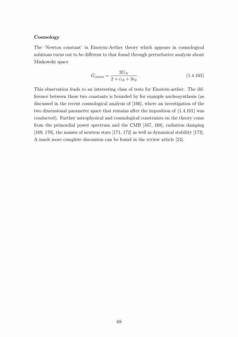
Cosmology

The ‘Newton constant’ in Einstein-Aether theory which appears in cosmological

solutions turns out to be different to that found through perturbative analysis about

Minkowski space

Gcosmo =2GN

2 + c13 + 3c2. (1.4.103)

This observation leads to an interesting class of tests for Einstein-aether. The dif-

ference between these two constants is bounded by for example nucleosynthesis (as

discussed in the recent cosmological analysis of [166], where an investigation of the

two dimensional parameter space that remains after the imposition of (1.4.101) was

conducted). Further astrophysical and cosmological constraints on the theory come

from the primordial power spectrum and the CMB [167, 168], radiation damping

[169, 170], the masses of neutron stars [171, 172] as well as dynamical stability [173].

A much more complete discussion can be found in the review article [24].

68

2. Bosonic Fractionalisation in

AdS/CFT

2.1. Introduction

In this chapter we will discuss a particular class of phase transition in condensed

matter physics known as fractionalisation transitions using the techniques of gauge

gravity duality. (The reader is referred to section 1.2.5 of the introductory chapter

of this thesis for an overview of the relevant aspects of applied holography). We

shall take a relativist’s approach to the subject, where the problem amounts to the

construction of particular classes of black hole solutions in general relativity and an

examination of their thermodynamics (so as to demonstrate the existence or non-

existence of a phase transition). In detail, we will have to solve the Einstein equations

in asymptotically AdS spacetime, in the presence of matter (which in our setting

will consist of an Abelian gauge field, together with a real and complex scalar). The

construction of such solutions is in general analytically intractable and one must

appeal to numerics. In this sense, this chapter constitutes our simplest example

of numerical relativity - the black holes that we construct are static and planar,

depending non-trivially only on a single (radial) coordinate so that the equations of

motion are ODEs. We will therefore not need the full elliptic formalism reviewed in

section 1.3 of the introduction, although we note extensions of this work where such

methods are invaluable. We proceed by solving the system using shooting methods,

constructing the black holes in a near horizon and asymptotic region respectively

and connecting the two. We begin with some condensed matter motivation and

an overview of what is meant by ‘bosonic fractionalisation’ before turning to the

problem of constructing the gravitational solutions.

In the context of condensed matter theory, given a field theory at finite density

(with respect to some U(1) symmetry), it is of interest to study the physical nature

of its ground states. In particular, one might be interested under what conditions the

U(1) symmetry is broken, corresponding to superfluid or superconducting phases,

if there are Fermi surfaces present and how their properties compare with those

69

of the conventional Fermi liquid theory that underlies much of modern solid state

physics. Such questions have attracted considerable interest recently, in particular

with regard to a classic result in condensed matter known as the Luttinger theorem

and a holographic generalisation thereof [174, 175, 176]. This result relates the sum

of the volumes of all Fermi surfaces Vi (associated to fermionic operators carrying

electric charge qi) to the total charge density Q1

Q =∑

i

qiVi . (2.1.1)

These studies were guided by the observation that the finite charge density of a field

theory, as encoded holographically by the electric flux in some dual gravitational

geometry can be sourced in two distinct ways: By explicit charged matter sources

in the bulk such as neutral ‘hairy black holes’ supporting charged scalar hair or al-

ternatively by the presence of charged black hole horizons with no hair2. (Note that

this distinction can be made technically sharp by virtue of the fact that the large

N limit of field theories that have gravity duals naturally involves a hierarchy be-

tween a small number of charged fields and a large quantity of black hole microstates

[177]). The case of a bulk charged horizon is of particular interest for condensed

matter - a fact that can be understood as a consequence of the holographic obser-

vation by Witten that the presence of a black hole horizon in the bulk geometry

is dual to deconfined phases of matter [178]. Using this as motivation, it has been

conjectured that electrically charged horizons may be used to describe field theories

in condensed matter where some of the electric charge density is tied up in ‘gauge-

variant’ operators, the flux from the horizon being associated with these deconfined

or ‘fractionalised’ charge carriers [8, 174]. The study of dual gravity geometries with

bulk horizons then serves as a powerful holographic tool to investigate such systems,

particularly when direct analysis of the field theory is intractable.

A useful system independent description of fractionalisation has been provided

by the Luttinger theorem [8]. In essence, since only Fermi surfaces corresponding

to gauge invariant degrees of freedom are experimentally observable (notably by

photoemission spectroscopy [174]), fractionalised gauge charge will show up as a

mismatch in the Luttinger theorem,

F = Q−∑

i

qiVi , (2.1.2)

1We note for completeness that there is also an analogous bosonic result that relates the totalcharge to the ‘Magnus force’ felt by some test vortex in the dual field theory [176].

2We stress in this latter case that these black holes are not hairy black holes. The charge isentirely ‘behind’ the black hole horizon with the charged scalar being zero outside.

70

where the amount the theorem is violated by corresponds to the electric flux F ema-

nating from a bulk horizon. Further support has been lent to this viewpoint recently

by the identification of the corresponding Green function singularities associated to

these ‘hidden’, fractionalised fermionic degrees of freedom in the work of Faulkner

and Iqbal [179].

A natural question to ask now is whether transitions can occur in physical systems

between phases which are fractionalised and phases which are not and it is this which

we now turn to for the remainder of this chapter. In gravitational language, we seek

transitions between solutions of the Einstein equations where the electric flux is

sourced entirely by a horizon (corresponding to full fractionalisation) and those

where it originates entirely due to charged matter in the bulk (corresponding to

what we call a cohesive phase) [174, 180, 181]. In the former case, this corresponds

to electrically charged bulk black holes without scalar hair and in the latter case to a

neutral black hole supporting charged scalar hair3. In addition to the aforementioned

phases one might also expect the existence of a partially fractionalised phase as

intermediate between these two extremes that corresponds on the gravity side to a

charged (as opposed to neutral) black hole supporting charged scalar hair. Since the

presence of non-singlet matter will always break the U(1) symmetry, such phases

have broken symmetry and hence the transition between a cohesive and partially

fractionalised phase must occur in the superfluid phase. In view of this, we will term

the two kinds of ordered phase in our subsequent work as the ‘superfluid cohesive

phase’ and the ‘superfluid fractionalised phase’.

Whilst violation of the Luttinger theorem as presented in equation (2.1.2) phrases

fractionalisation in terms of fermionic systems, for the remainder of this chapter

we will in fact discuss gravitational duals to bosonic fractionalisation transitions

that serve as bosonic analogues of the fermionic transitions discussed in [174, 182].

That is to say, the holographic gravitational actions we consider will consist of

only bosonic fields. In detail, we shall discuss fractionalisation both in an ad-hoc

(‘bottom-up’) Einstein-Maxwell-dilaton-charged scalar theory as well as (briefly) in

a top-down’ model that arises as a reduction of 11D supergravity (the low energy

limit of M-theory). As we shall see, the fractionalisation transitions that can occur in

these settings constitute rather striking zero temperature quantum phase transitions

that leave a marked imprint on finite temperature physics4. We note also that the

3Such a transition has already been observed in the literature, namely the M-theory superconduc-tor transition from finite temperature charged black hole to zero temperature charged domainwall with no horizon. We shall discuss this in further detail in what follows.

4Indeed the study of such T = 0 quantum critical points is of great theoretical interest in con-densed matter more generally as they are believed to play a role in various ill understoodphenomena notably high temperature superconductivity [7].

71

gravitational theories we consider share a structural similarity to those discussed

in the electron star literature [183] with the charged scalar taking the place of the

fermion fluid found there. Some of the infrared (IR) geometries considered there

will also feature in our work. Similar solutions have also previously found use in the

description of QCD like theories [184, 185, 186] and in the description of quantum

criticality at finite density [187, 188, 189, 190, 191, 192, 193, 194].

In detail, we begin by introducing the class of Einstein-Maxwell-dilaton-charged

scalar theories we will consider for the remainder of this chapter. We then develop

the holographic renormalisation and thermodynamics of these models in some detail

with a view to calculating the free energy which is of crucial importance for phase

transition physics. We then provide a detailed description of a class of bottom-up

models which illustrate the concepts underlying fractionalisation and use shooting

methods to construct T = 0 solutions of these models that are dual to fractionalised,

partially fractionalised and cohesive phases in field theory. Finally, we close by

outlining aspects of fractionalisation at finite temperature and in a top-down M-

theory setting. (The latter two topics are discussed in much greater length in the

paper on which this chapter is based [2]).

The main results of our analysis are summarised in Fig. 2.1. In particular, as we

shall see, the phase diagram is governed by the structure of the IR zero temperature

states. Depending on the nature of the effective gauge coupling which is controlled

by the neutral scalar field, we find either a fully or partially fractionalised phase, if

the coupling goes to zero and a cohesive phase if it remains finite. In the latter two

cases, as explained above, the U(1) symmetry is manifestly broken, so we end up

with superfluid states of matter. In addition to the aforementioned phases, there is

one further neutral phase that arises in the M-theory case, where the ground state

does not depend on the chemical potential (it is ‘incompressible’). In fact, the only

T = 0 phase transition in the M-theory case is governed by a z = 2 quantum critical

point and is from cohesive to neutral (and is not a fractionalisation transition).

2.2. General Features, Action and Field Content

In this section, we introduce the gravitational theories we will be concerned with

in a setting general enough to cover both bottom-up and top-down constructions.

At zero temperature we will analyse the possible IR geometries admitted by these

theories as well as the deformations about these solutions that allow them to be

connected to the desired AdS asymptotics (that will be universal to everything

we shall consider in this chapter). As we shall see, these IR geometries are zero

72

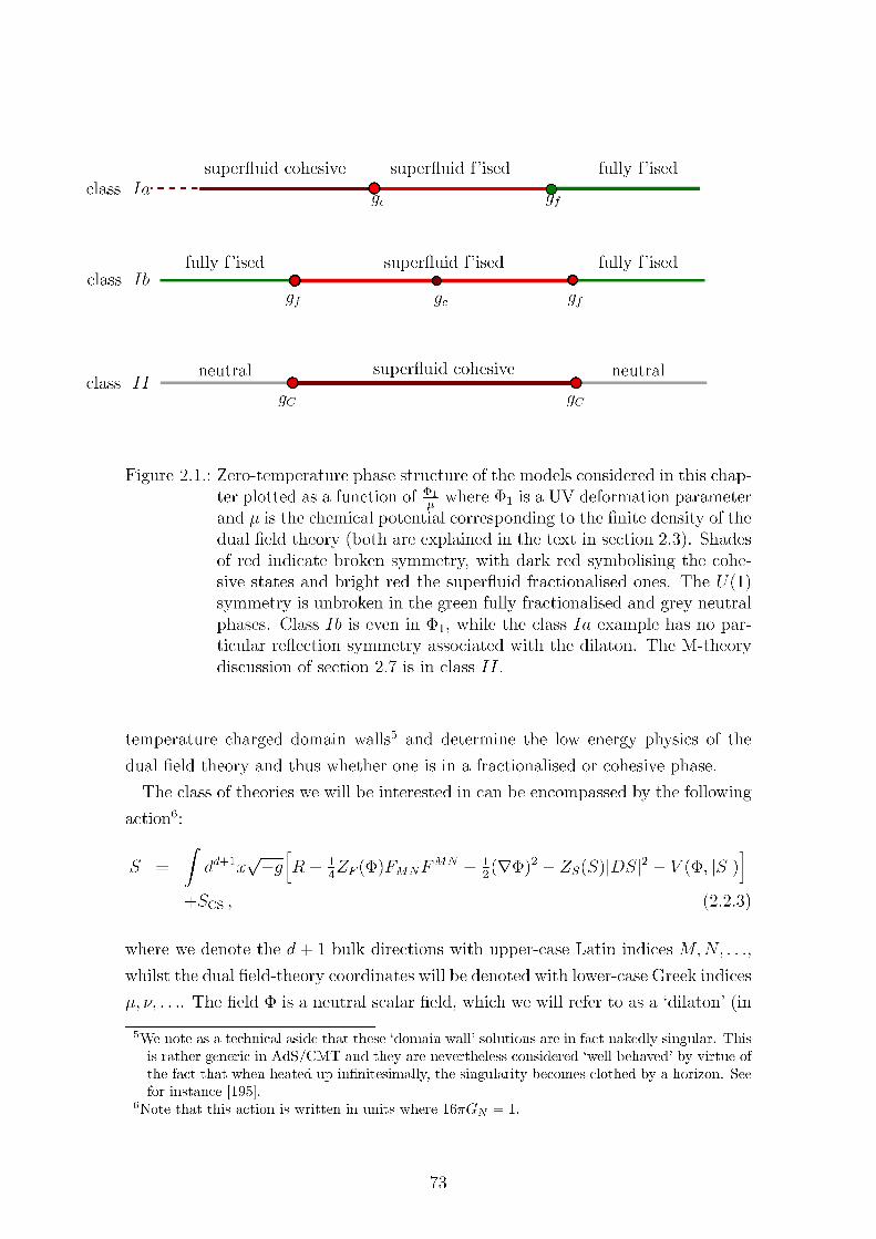
the spirit of string theory), whereas S is a charged scalar field with the usual U(1)

covariant derivative DS = (∇ − iqA)S. We have also included a term SCS, which

stands for a possible Chern-Simons contribution. These are often found in consistent

supergravity reductions and are relevant in top-down constructions. Whilst the

solutions we construct will not depend on SCS, we note that in certain cases the

phase structure may be altered by its presence, and spatial modulation and striped

phases become possible [196, 197, 198, 199]. This will not be discussed further here

although we note that in these cases, the black hole ansatz that must be solved for

results in PDEs and the elliptic techniques of section 1.3 have recently taken centre

stage in this area of holography (see for example [200]).

The coupling coefficients ZF (Φ), ZS(S) as well as the potential term V (Φ, |S|)in the action (2.2.3) depend explicitly on the neutral and complex scalar fields.

(Note that we have not considered the most general action of this form here, but

it is sufficient to capture the physics we wish to discuss). In a ‘bottom-up’ setting,

these quantities are not specified by some underlying fundamental theory and must

be chosen ‘by hand’. Much of the interesting behaviour we will exhibit in these

theories depends on this choice and arises as a consequence of the interplay between

the potential and couplings. It will be convenient to recast the kinetic terms for the

scalars in canonical form, (although this is in fact only possible for the magnitude of

the complex field). We can rewrite the kinetic term for the charged scalar S using

a polar decomposition as S = η′eiqϕ and compute that

ZS(|S|)|DS|2 = ZS(η′)(∇η′)2 + q2ZS(η

′)η′2(∇ϕ− A)2 . (2.2.4)

On changing variables to η, defined as∫dη′√

Zs(η′) =∫dη, one then arrives at

ZS(|S|)|DS|2 = (∇η)2 + q2X(η)2(∇ϕ− A)2 , (2.2.5)

where we have introduced a function X(η) which arises due to the aforementioned

change of variables. It is required to have the small-η expansion X(η) ∼ η +O(η2).

We now make some further simplifications to the action (2.2.3). In the ‘bottom-up’

analysis that follows,X(η) must be specified (this is of course equivalent to specifying

ZS(S)). We may in fact capture all the physics we wish to discuss by retaining only

the first term in the above small-η expansion and shall do so in what follows. (We

discuss the more general case here as in the ‘top-down’ M-theory case, a closed form

expression for ZS(S) and hence X(η) is known from dimensional reduction which

may then be included in full in calculations). We may now use the local U(1) gauge

symmetry in the theory to transform S → eiθS (equivalently η → η, ϕ → ϕ + θ/q)

74

together with A → A + ∂θ/q. Using this we can (by a suitable choice of θ) fix a

gauge where ϕ = 0 and we shall do this in what follows.

The general action we consider (in terms of real fields) is then of the form,

S =

∫

dd+1x√−g

[

R− 14ZF (Φ)FMNF

MN − 12(∇Φ)2 − (∇η)2

−q2X(η)2A2 − V (Φ, |S|)]

, (2.2.6)

where X(η) = η by choice in the ‘bottom-up’ case with ZF (Φ) and V (Φ, |S|) to

be specified later. All these aforementioned quantities are fixed by dimensional

reduction in ‘top-down’ constructions.

Of particular interest in holography are the so called hyperscaling geometries.

These are defined in terms of the following scaling symmetry which should be

thought of as a generalisation of the Lifshitz scaling reviewed in the introduction

(see section 1.2.5):

x → λx ,

t → λzt ,

r → λ(θ−2)/2r , (2.2.7)

under which ds → λθ/2ds. Here, z is the dynamical critical exponent present in

the Lifschitz case, and θ is the new hyperscaling violation parameter. Hyperscaling

is physically significant, influencing the thermodynamics of gravitational solutions.

Recently it has also been realised that theories with hyperscaling violation can ex-

hibit intriguing violations of area laws for entanglement entropy (intermediate be-

tween linear and logarithmic violation) perhaps indicating the existence of duals to

novel, exotic phases of matter [194]). Hyperscaling geometries are generated by an

IR divergent dilaton (Φ −→ ±∞)[191, 192, 193], and so in classifying solutions of

our theory it will be important to first classify the possible behaviours of the dila-

ton in the IR (and hence the behaviour of the coupling ZF (Φ)). We consider two

possibilities defined as follows:

class I : ZF (Φ)IR−−−−−→ ∞ ,

class II : ZF (Φ)IR−−−−−→ Constant . (2.2.8)

We emphasise that we do not require ZF (Φ) to be even in Φ. In particular, this is

of importance in class I, where one can envision a scenario where ZF (Φ) diverges as

say Φ −→ ∞, but remains finite as Φ −→ −∞. As we shall see, it is in this sense

75

that Φ is able to drive fractionalisation type transitions.

Finally, we must specify the potential, which we require to have an expansion of

the following form

ℓ2V (η,Φ) = −6− Φ2 − 2η2 + · · · (2.2.9)

The first term is chosen to ensure that we have an AdS4 vacuum solution with AdS

length l2 when all fluxes vanish (it is essentially a cosmological constant term) and

the remaining terms can be thought of as fixing the conformal dimension (∆ = 2)

of the dual operators to the Φ and S fields.

For the remainder of this chapter we work in D = 4 bulk dimensions, so that the

boundary field theory is d = 3 dimensional. We will use the following ansatz for the

metric, gauge and scalar fields. Note that all functions depend only on the radial

coordinate r. t, x, y are field theory coordinates and we remind the reader, that

the r coordinate corresponds to the ‘extra’ dimension in the bulk geometry which

has a holographic interpretation in terms of field theory energy scale (as discussed

previously in section 1.2.5),

ds2 = −f(r)e−β(r)dt2 +dr2

f(r)+r2

ℓ2(dx2 + dy2

),

A = At(r)dt , Φ = Φ(r) , η = η(r) . (2.2.10)

The metric above has a horizon at r = rh defined by f(rh) = 0, and on this

hypersurface we must also impose the condition At(rh) = 07. Evaluated on our

ansatz (2.2.10), the equations of motion following from (2.2.6) are found to be:

0 = Φ′′ +

(f ′

f− 1

2β′ +

2

r

)

Φ′ +(∂ΦZF )A

′2eβ

2f− ∂ΦV

f,

0 = η′′ +

(f ′

f− 1

2β′ +

2

r

)

η′ +q2A2eβ

f 2η − ∂ηV

2f,

0 = A′′ +

(Z ′

F

ZF

+1

2β′ +

2

r

)

A′ − 2q2η2

fZF

A ,

0 = Φ′2 + 2η′2 +2q2A2η2eβ

f 2+

2

rβ′ ,

0 = Φ′2 + 2η′2 +2q2A2η2eβ

f 2− 2V

f− 4

r

(f ′

f− β′ +

1

r

)

− 2A′2eβ

f.

(2.2.11)

7One way to understand this condition is by continuing to Euclidean signature as we shall do inour discussion of thermodynamics. One can then argue that we would obtain a singular gaugeconnection on integrating the gauge field around the Euclidean time circle if we did not haveAt → 0 as the Euclidean time circle shrinks to zero at the horizon.

76

2.3. Ultraviolet Expansions and Asymptotic

Charges

Following standard AdS/CFT technology, we require solutions that asymptote to

AdS4 at large values of r. From the field equations that follow from (2.2.3) one finds

that such solutions admit the large r expansions:

f =r2

ℓ2+

1

2

(η21 +

12Φ2

1

)+ℓG1

r+ · · · ,

β = βa +ℓ2(η21 +

12Φ2

1

)

2r2+ · · · ,

Φ =ℓΦ1

r+ℓ2Φ2

r2+ · · · ,

η =ℓη1r

+ℓ2η2r2

+ · · · ,

At = ℓe−βa/2

(

µ− Q

r+ · · ·

)

, (2.3.12)

where there are eight undetermined integration constants Φ1,Φ2, η1, η2, µ,Q,G1, βaknown as UV data in these expansions. The ellipses denote terms higher order in

1/r, the coefficients of which are determined entirely in terms of the aforementioned

eight pieces of UV data. By application of the holographic dictionary, we can relate

the data that enters the leading and subleading fall-offs of the Φ(r) and η(r) equa-

tions to the source and VEVs of the operators dual to these fields in the boundary

theory. The data µ and Q correspond respectively to the chemical potential and

charge density associated to the finite density of the field theory. Finally, by con-

structing the boundary stress tensor one can deduce the exact relationship between

the remaining UV data in these expansions and thermodynamic quantities such as

the energy and pressure of the dual theory. This procedure is knows as holographic

renormalisation as it involves as a first step the addition of counterterms to (2.2.3)

to render the full on shell action finite. There is no ambiguity in the ‘gravitational

part’ of this counterterm action, however, for the scalars one must make a choice

(corresponding to whether one imposes Dirichlet or Neumann conditions for the

second order scalar equation). We choose counterterms for the scalar fields such

that the fixed η1,Φ1 ensemble has a well defined variational principle. The specific

counterterm action we choose is

Sct = 2

∫

∂Σ

√−γ(

K − 2

ℓ

)

−∫

∂Σ

√−γ 1ℓ

(|S|2 + 1

2Φ2), (2.3.13)

77

where K = γµνKµν is the trace of the extrinsic curvature of a constant r hypersurface

with unit normal nr = f(r)12 and γµν is the induced metric on such a slice. We then

find that the total renormalised action

Sren = S + Sct (2.3.14)

is finite, as is the renormalised stress tensor (obtained by functional differentiation

of the renormalised action)

Tµν = −2δSren

δγµν= 2

(

Kµν −Kγµν −2

ℓγµν

)

− 1

ℓ

(|S|2 + 1

2Φ2)γµν . (2.3.15)

From the stress tensor, we can then extract the energy density8 of the field theory

defined as

ε =reβa

ℓT00 = −2

ℓ

(G1 − η1η2 − 1

2Φ1Φ2

). (2.3.16)

We pause at this point to emphasise the very different roles played by the two scalar

fields in our theory. The dilaton Φ introduces an explicit deformation parameter

into the theory. More explicitly, we can switch on a relevant operator by sourcing

it in the dual theory - in other words by choosing a non-zero value for the UV

expansion parameter Φ1. In contrast, we do not want to allow the second scalar

η to act as a source as we would like to consider situations where it can condense

spontaneously (corresponding to superconductivity in field theory) and hence shall

ultimately impose η1 = 0 in what follows.

2.4. Thermodynamics

We now turn to a discussion of the thermodynamics of gravitational solutions and

relate this to the asymptotic charges of the previous section. In order to do this we

begin by analytically continuing to Euclidean signature9

t = −iτ , IE = −iSren , AEτ (r) = −iAt(r) , (2.4.17)

8The quantity e−βa is the boundary speed of light (squared), and so the conversion between ADMmass and energy, and correspondingly energy density, involves a factor of e−βa . For this andrelated reasons it is convenient to set βa = 0, which we will assume to be the case from nowon.

9We emphasise in the interest of clarity that all calculations in this section will be Euclidean butthe discussion in this chapter up to this point has of course been Lorentzian and in subsequentsections will return to that signature.

78

where the index E stands for Euclidean. As a starting point for thermodynamics,

we work in the grand canonical ensemble where the Euclidean action IE is related

to the (Gibbs) free energy Ω(µ, T ) as

IE = βΩ(µ, T ) := βvol2ω(µ, T ) , (2.4.18)

where the second equality is to be regarded as a definition of the quantity ω(µ, T ).

The key result from which all the thermodynamic relations we are interested in

follow is that when evaluated on-shell (i.e. assuming that the equations of motion

are satisfied), the above action can be written as a total derivative. We now outline

how one can arrive at this fact: one begins by observing after a direct calculation

that the (x, x) component of the stress energy tensor Tµν = −2 δLM

δgµνcan be written

as

Txx =r2

l2(L −R) , (2.4.19)

where R is the Ricci scalar for the geometry (2.2.10) and L is the Lagrangian density

(defined by S =∫d4x√

|g|L =∫d4x√

|g| (R + LM)) for the action (2.2.3). The

corresponding component of the Einstein tensor Gµν = Rµν − 12gµν is then given by

Gxx = gxxGxx =

1

2(L −R) , (2.4.20)

where we have used the Einstein equations Gxx = 12Txx (and we remind the reader

that the factor of 12arises as we are working in units where 16πG = 1). Using the

result that R = −Gµµ, we then arrive at

L = −(Gττ +Gr

r), (2.4.21)

and hence

SOS = −∫√

|g| (Gττ +Gr

r) ddx , (2.4.22)

where SOS is the on-shell action. One may now show by explicit calculation of the

Einstein tensor (on our ansatz (2.2.10)) that

∫√

|g| (Gττ +Gr

r) ddx = −iβvol2

∫ ∞

r+

d

dr

[2

r

√

|g|grr]

dr , (2.4.23)

from which we see that the on shell action is indeed a total derivative as claimed.

We have introduced a lower limit in the above integral to account for a possible

black hole horizon in the IR of the geometry at r = r+. (We are implicitly assuming

79

we are using bulk coordinates which are only valid exterior to a horizon and hence

the lower limit of the integration should be cut off at this radial position). In fact

(2.4.23) vanishes when evaluated there as grr = 0, and hence the integral only has

an asymptotic contribution at infinity.

Using the above expression for IOS, one can now calculate quantities such as the

pressure of the system using standard thermodynamic relations

ω(µ, T ) = −P . (2.4.24)

We conclude our discussion of thermodynamics with a derivation of the Smarr re-

lation for our system. We may exploit the symmetries of the background metric,

to show that this follows from the vanishing of another total derivative on shell. In

particular, note that we have two commuting Killing vectors T = ∂τ , ν = ∂y. For κ

Killing, we have the Ricci identity RMNkM = ∇M∇Nk

M , from which we conclude

that

√

|g|RMNk

N = −∂r(√

|g|grN∇NkM) , (2.4.25)

where we have used the Killing equation as an intermediate step.

In this way, we construct

√

|g|Rττ =

√

|g|RτMT

M = −∂r[e−β/2r2

2l2(fβ′ − f ′)

]

, (2.4.26)

√

|g|Ryy =

√

|g|RyMν

M = ∂r

[e−β/2rf

l2

]

, (2.4.27)

and hence

√

|g| (Rττ −Ry

y) = −∂r[e−β/2r2

2ℓ2

(

fβ′ − f ′ +2f

r

)]

. (2.4.28)

The trace reversed Einstein equations can now be used to obtain the following (on

shell) relation

√

|g| (Rττ −Ry

y) = −1

2∂r

[√

|g|ZF (Φ)AEτ F

τr]

. (2.4.29)

Note that whilst the construction of (2.4.28) is carried out systematically using the

symmetries of the background spacetime, in the derivation of (2.4.29), it is a matter

of trial and error to find the correct linear combination to give a total derivative.

Integration from the black hole horizon at r = r+ to the UV boundary at r = ∞

80

gives the result

e−β/2r2

ℓ2

(

fβ′ − f ′ +2f

r

)∣∣∣∣∣

∞

r+

=√

|g|ZF (Φ)AEτ F

τr∣∣∣

∞, (2.4.30)

where the bottom limit on the right hand side vanishes as AEτ (rh) = 0 as discussed

previously. Evaluated on our UV expansions, we then obtain the Smarr-Gibbs-

Duhem relation3

2ε = µQ+ Ts− ℓ−1

(

η1η2 +1

2Φ1Φ2

)

, (2.4.31)

which can be rewritten in terms of the pressure P , charge density Q, and Hawking

temperature T as

ε+ P = µQ+ Ts , (2.4.32)

where we have used that the fact that the temperature is given by

T =e(βa−β+)/2

4πℓ2f ′(r)

∣∣∣r=r+

(βa = 0) , (2.4.33)

and moreover, the entropy density is given in terms of the horizon radius as

s =r2+4GN

(note 16πGN = 1) . (2.4.34)

Whilst we have performed the above thermodynamic calculations at finite temper-

ature, it is important to emphasise that they continue to hold at zero temperature

(where r+ → 0). Indeed it is this case that is of most relevance for the discussion

that follows in this thesis where the expression for the pressure (and hence Gibbs

free energy) is important in demonstrating the existence of T = 0 phase transitions.

2.5. Class I: Bottom Up Model and T = 0

Shooting Problem

Having analysed the asymptotic AdS4 expansions and thermodynamics of the so-

lutions we are concerned with for the last two sections, we will now begin our

discussion of how to set up the numerical problem of connecting this AdS4 struc-

ture to IR geometries that describe fractionalised and cohesive phases of matter.

This will constitute a shooting problem and we will have to develop IR expansions

of the field equations (in analogy to what was done in the UV) about leading or-

der geometries that describe fractionalised or cohesive phases respectively. We will

81

perform this analysis at zero temperature where these leading order geometries are

singular, charged domain walls. (They are ‘well-behaved’ nevertheless in the sense

that they are the zero temperature limit of non-singular black holes with horizons

at finite temperature [2]). Before turning to their construction, however, we first

make precise the class of models we will be interested in by a further specialisation

of the action (2.2.3).

In the case where ZF (Φ) is not symmetric in Φ, there are two qualitatively different

behaviours associated with a divergent dilaton. When the dilaton diverges to plus

(minus) infinity, the effective gauge coupling e2 ∼ Z−1 goes to zero (infinity) in

the IR. This behaviour is crucial in our discussion, and in particular as we shall

see, it is this that gives rise to a continuous phase transition between a superfluid

fractionalised phase and a cohesive phase, via a quantum critical point with finite

dilaton. (The transition being driven by the asymptotic (UV) value of the dilaton

Φ1). We will also demonstrate that the gravitational solutions on either side of this

solution are of hyperscaling form. In addition to the aforementioned fractionalisation

transition, there is also a further transition between a partial and fully fractionalised

phase that we shall also discuss.

In order to proceed with our analysis we will now specialise our theory to a

particular sub-class of models, sufficient to display the physics we are interested in,

by specification of the coupling functions ZF (Φ) and V (Φ, η). We choose,

ZF (Φ) = Z20e

aΦ/√3 , ℓ2V (Φ, η) = −V 2

0 cosh(

bΦ/√3)

− 2η2 + g2ηη4 , (2.5.35)

where a, b > 0 (the latter condition is of course without loss of generality). The

η4 term allows for soliton solutions that interpolate between the AdS4 maximum at

η = 0 and the AdS4 minimum at η2 = g−2η . We will study IR geometries for general

values of a and b (see also [174, 182]). All our numerical results will however be for

the particular case a = b = g2η = 1, V 20 = 6 and Z2

0 = 1.

2.5.1. T=0 Infrared Expansions

We now develop IR expansions of the equations of motion that follow from (2.2.3)

about geometries describing fractionalised and cohesive states of matter. We work at

T = 0 and following Hartnoll [174] expand all fields in a Frobenius expansion about

r = 0. Moreover, we search for solutions that have a logarithmically divergent

82

dilaton10. In summary, we look for expansions about r = 0 of the form:

f(r)e−β(r) = rα

(

1 +∞∑

n=1

βnrsn

)

,

f(r) = f0rβ

(

1 +∞∑

n=1

fnrsn

)

,

At(r) = A0rγ

(

1 +∞∑

n=1

Anrsn

)

,

Φ(r) =√3

(

δ log r +∞∑

n=1

Φnrsn

)

,

η(r) = η0rτ

(

1 +∞∑

n=1

Πnrsn

)

, (2.5.36)

where α, β, γ, δ, τ, f0, A0, η0, βn, fn, An,Φn,Πn are constants to be determined by

solving the equations of motion order by order and s ∈ is the step-size of the series.

We note that we have used a rescaling of the t coordinate to remove a constant pre-

factor in the f(r)e−β(r) expansion together with an r rescaling to remove a constant

term in the Φ(r) expansion. The quantities α, β, γ, δ, τ, f0, A0, η0 characterise the

leading order solution. As we shall see in the next subsection, in the case of a

fractionalised IR solution (where the IR horizon flux is non-vanishing), the quantities

α, β, γ, δ, τ, f0, A0 are explicitly determined by the equations of motion at leading

order. On the other hand, η0 is not determined at this order and is data. The

remaining coefficients in the expansions βn, fn, An,Φn,Πn are fully determined at

higher orders and no new data enters the system. In the case of a cohesive solution,

together with the equations of motion, we impose that the horizon flux vanishes in

the IR (limr→0

√−gZ(Φ)F rt = 0). One finds then that α, β, δ, τ, f0 are determined

by the leading order equations of motion, whilst A0 and η0 are data (γ which is free

at this order gets fixed in terms of η0 when including perturbations as we explain

below). In order to ensure the IR horizon flux vanishes, we set A0 = 0 for our

cohesive solutions. (Note we will later introduce a non-zero flux into these solutions

by including deformations about them as we describe in the next paragraph). As

with the fractionalised solutions, all the higher order coefficients βn, fn, An,Φn,Πnare determined order by order and there is no more data.

Having developed the IR expansions above, we need to connect them to the AdS4

asymptotics of section (2.3). In order to do this, we proceed by perturbing the IR

10As explained above, the heuristic motivation for choosing this behaviour is that the divergenceof Φ controls the behaviour of ZF (Φ) and thus the effective gauge coupling and bulk IR electricflux, which is intimately tied to fractionalisation.

83

expansions above11. This perturbed expansion can then be integrated outwards (to

large values of r) and connected to the UV expansion (that is integrated inwards)

by tuning a subset of the IR and UV data as a shooting problem. (The shooting

problem itself will be described in much greater detail in the next section). We

perturb the equations (2.5.36) as follows,

f(r)e−β(r) = rα

(

1 +∞∑

n=1

βnrsn

)

+ ǫrα δβ

( ∞∑

ij=1

βijriN+s(j−1)

)

,

f(r) = f0rβ

(

1 +∞∑

n=1

fnrsn

)

+ ǫrβ δf

( ∞∑

ij=1

fijriN+s(j−1)

)

,

At(r) = A0rγ

(

1 +∞∑

n=1

Anrsn

)

+ ǫrγ δA

( ∞∑

ij=1

AijriN+s(j−1)

)

,

Φ(r) =√3

(

δ log r +∞∑

n=1

Φnrsn

)

+ ǫ√3 δΦ

( ∞∑

ij=1

ΦijriN+s(j−1)

)

,

η(r) = η0rτ

(

1 +∞∑

n=1

Πnrsn

)

+ ǫrτ δη

( ∞∑

ij=1

ηijriN+s(j−1)

)

, (2.5.37)

where ǫ is the expansion parameter and N, δβ, δf, δA, δΦ, δη, βij, fij, Aij,Φij, ηijare constants. The leading perturbations about our original IR background are

characterised by an exponent N and amplitudes δβ, δf, δA, δΦ, δη. (Without loss

of generality, we have assumed that β11 = f11 = A11 = Φ11 = η11 = 1). These

quantities can be determined by the linearisation of the equations of motion, about

the background (2.5.36) including only the leading perturbation in (2.5.37). (More

than the leading term should of course be included when shooting later). In more

detail, if we substitute this expansion into the equations of motion, which we write

as a vector Ei (consisting of the Einstein, Maxwell and scalar equations) and then

expand as a power series in ǫrN , one finds (at leading order)

Mijδvj = 0 , (2.5.38)

where vj = β(r), f(r), At(r),Φ(r), η(r), δvj = δβ, δf, δA, δΦ, δη and the lin-

earisation of the equations Mij =δEi

δvj. The exponent N is then determined by the

condition detMij = 0 and the vector δvj is given by the zero eigenvectors ofMij. The

equation governing the perturbations (2.5.38) admits two non-trivial solutions for

the IR backgrounds we discuss. In the fractionalised case, for the first deformation

11In holographic language, we would like to characterise the possible irrelevant deformations aboutthe IR solution (2.5.36) and use these to induce an RG flow to the UV.

84

one finds that N is determined explicitly, all perturbation modes except the charged

scalar are excited (δη = 0) and δvj is given in terms of a single free parameter cIR.

The second deformation on the other hand has N = 0 and perturbs only the IR value

of the charged scalar. In total therefore, there are two pieces of IR data in fraction-

alised solutions: η0 and cIR. For cohesive solutions, the situation is somewhat more

complex and one finds for the first perturbation that N = N(η0), and furthermore

γ = γ(η0) (recall γ was not fixed at leading order in the cohesive case). The only

mode that is excited is the Maxwell field mode, (so δβ = δf = δΦ = δη = 0). The

second perturbation has N = 0 and shifts the IR value of the charged scalar only.

In total, as with the fractionalised case, there are hence two pieces of IR data: η0

and δA. We now present in more detail the IR geometries that we have found.

Fractionalised IR Solutions

The first class of solutions we discuss are fractionalised solutions, where some or all

of the flux is sourced by a black hole horizon. In this case, one must demand that

the horizon flux√−gZ(Φ)F rt is a non-zero constant as r → 0. This is most easily

engineered by substituting the expansions (2.5.36) into the horizon flux, to find at

leading order√−gZ(Φ)F rt ∼ r1+

12(α−β)+δ+γ . To ensure a non-zero horizon flux, we

then impose that 1+ 12(α−β)+ δ+γ = 0. The fractionalised IR solutions are found

to be

f(r)e−β(r) = r2(12+a2−b2)

(a+b)2

(

1 +∞∑

n=1

βnrsn

)

,

f(r) = f0r2(a−b)a+b

(

1 +∞∑

n=1

fnrsn

)

,

At(r) = A0r12+(3a−b)(a+b)

(a+b)2

(

1 +∞∑

n=1

Anrsn

)

,

Φ(r) =√3

(

−4

a+ blog r +

∞∑

n=1

Φnrsn

)

,

η(r) = η0rτ

(

1 +∞∑

n=1

Πnrsn

)

, (2.5.39)

where

f0 =(a+ b)4V 2

0

4(6 + a(a+ b))(12 + (3a− b)(a+ b)),

A20 =

4(6− b(a+ b))

(12 + (3a− b)(a+ b))Z20

. (2.5.40)

85

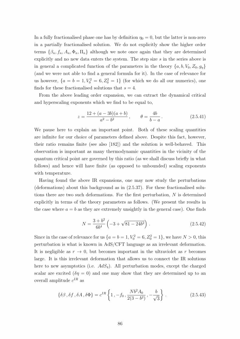
In a fully fractionalised phase one has by definition η0 = 0, but the latter is non-zero

in a partially fractionalised solution. We do not explicitly show the higher order

terms βn, fn, An,Φn,Πn although we note once again that they are determined

explicitly and no new data enters the system. The step size s in the series above is

in general a complicated function of the parameters in the theory a, b, V0, Z0, gη(and we were not able to find a general formula for it). In the case of relevance for

us however, a = b = 1, V 20 = 6, Z2

0 = 1 (for which we do all our numerics), one

finds for these fractionalised solutions that s = 4.

From the above leading order expansion, we can extract the dynamical critical

and hyperscaling exponents which we find to be equal to,

z =12 + (a− 3b)(a+ b)

a2 − b2, θ =

4b

b− a. (2.5.41)

We pause here to explain an important point. Both of these scaling quantities

are infinite for our choice of parameters defined above. Despite this fact, however,

their ratio remains finite (see also [182]) and the solution is well-behaved. This

observation is important as many thermodynamic quantities in the vicinity of the

quantum critical point are governed by this ratio (as we shall discuss briefly in what

follows) and hence will have finite (as opposed to unbounded) scaling exponents

with temperature.

Having found the above IR expansions, one may now study the perturbations

(deformations) about this background as in (2.5.37). For these fractionalised solu-

tions there are two such deformations. For the first perturbation, N is determined

explicitly in terms of the theory parameters as follows. (We present the results in

the case where a = b as they are extremely unsightly in the general case). One finds

N =3 + b2

6b4

(

−3 +√81− 24b2

)

. (2.5.42)

Since in the case of relevance for us a = b = 1, V 20 = 6, Z2

0 = 1, we have N > 0, this

perturbation is what is known in AdS/CFT language as an irrelevant deformation.

It is negligible as r → 0, but becomes important in the ultraviolet as r becomes

large. It is this irrelevant deformation that allows us to connect the IR solutions

here to new asymptotics (i.e. AdS4). All perturbation modes, except the charged

scalar are excited (δη = 0) and one may show that they are determined up to an

overall amplitude cIR as

δβ , δf , δA , δΦ = cIR

1 ,−f0 ,Nb2A0

2(3− b2),− b√

3

. (2.5.43)

86

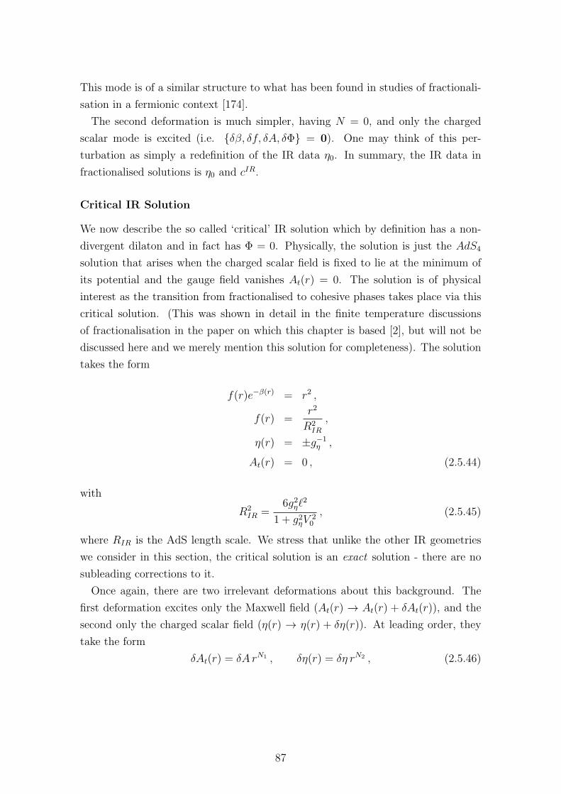
This mode is of a similar structure to what has been found in studies of fractionali-

sation in a fermionic context [174].

The second deformation is much simpler, having N = 0, and only the charged

scalar mode is excited (i.e. δβ, δf, δA, δΦ = 0). One may think of this per-

turbation as simply a redefinition of the IR data η0. In summary, the IR data in

fractionalised solutions is η0 and cIR.

Critical IR Solution

We now describe the so called ‘critical’ IR solution which by definition has a non-

divergent dilaton and in fact has Φ = 0. Physically, the solution is just the AdS4

solution that arises when the charged scalar field is fixed to lie at the minimum of

its potential and the gauge field vanishes At(r) = 0. The solution is of physical

interest as the transition from fractionalised to cohesive phases takes place via this

critical solution. (This was shown in detail in the finite temperature discussions

of fractionalisation in the paper on which this chapter is based [2], but will not be

discussed here and we merely mention this solution for completeness). The solution

takes the form

f(r)e−β(r) = r2 ,

f(r) =r2

R2IR

,

η(r) = ±g−1η ,

At(r) = 0 , (2.5.44)

with

R2IR =

6g2ηℓ2

1 + g2ηV20

, (2.5.45)

where RIR is the AdS length scale. We stress that unlike the other IR geometries

we consider in this section, the critical solution is an exact solution - there are no

subleading corrections to it.

Once again, there are two irrelevant deformations about this background. The

first deformation excites only the Maxwell field (At(r) → At(r) + δAt(r)), and the

second only the charged scalar field (η(r) → η(r) + δη(r)). At leading order, they

take the form

δAt(r) = δA rN1 , δη(r) = δη rN2 , (2.5.46)

87

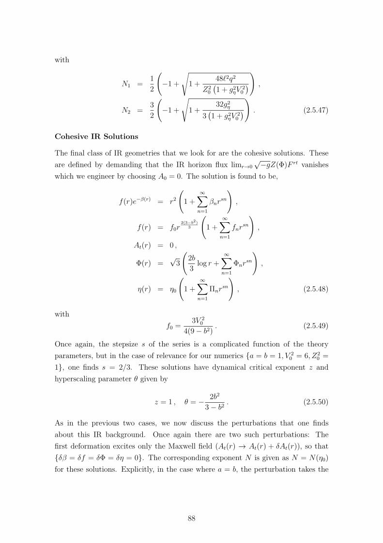
with

N1 =1

2

(

−1 +

√

1 +48ℓ2q2

Z20

(1 + g2ηV

20

)

)

,

N2 =3

2

(

−1 +

√

1 +32g2η

3(1 + g2ηV

20

)

)

. (2.5.47)

Cohesive IR Solutions

The final class of IR geometries that we look for are the cohesive solutions. These

are defined by demanding that the IR horizon flux limr→0

√−gZ(Φ)F rt vanishes

which we engineer by choosing A0 = 0. The solution is found to be,

f(r)e−β(r) = r2

(

1 +∞∑

n=1

βnrsn

)

,

f(r) = f0r2(3−b2)

3

(

1 +∞∑

n=1

fnrsn

)

,

At(r) = 0 ,

Φ(r) =√3

(

2b

3log r +

∞∑

n=1

Φnrsn

)

,

η(r) = η0

(

1 +∞∑

n=1

Πnrsn

)

, (2.5.48)

with

f0 =3V 2

0

4(9− b2). (2.5.49)

Once again, the stepsize s of the series is a complicated function of the theory

parameters, but in the case of relevance for our numerics a = b = 1, V 20 = 6, Z2

0 =

1, one finds s = 2/3. These solutions have dynamical critical exponent z and

hyperscaling parameter θ given by

z = 1 , θ = − 2b2

3− b2. (2.5.50)

As in the previous two cases, we now discuss the perturbations that one finds

about this IR background. Once again there are two such perturbations: The

first deformation excites only the Maxwell field (At(r) → At(r) + δAt(r)), so that

δβ = δf = δΦ = δη = 0. The corresponding exponent N is given as N = N(η0)

for these solutions. Explicitly, in the case where a = b, the perturbation takes the

88

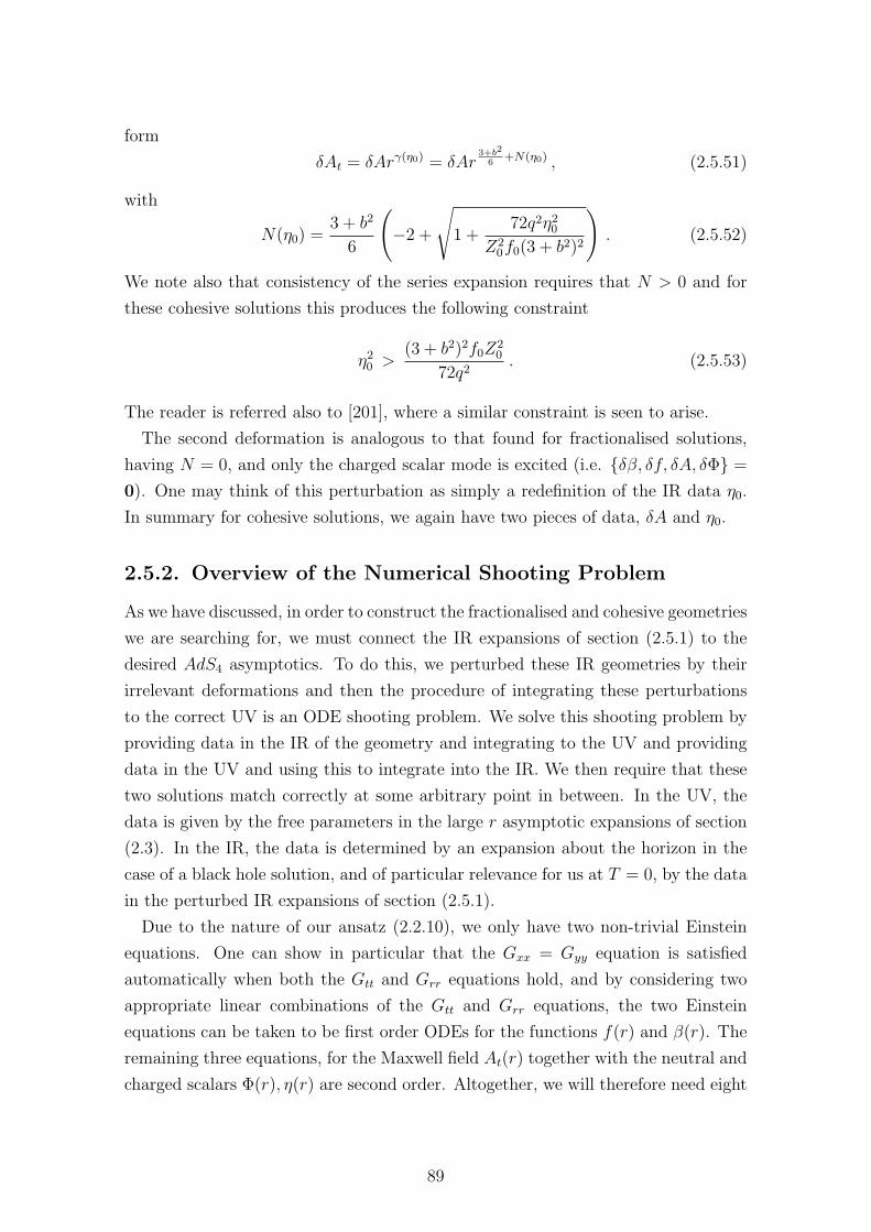
form

δAt = δArγ(η0) = δAr3+b2

6+N(η0) , (2.5.51)

with

N(η0) =3 + b2

6

(

−2 +

√

1 +72q2η20

Z20f0(3 + b2)2

)

. (2.5.52)

We note also that consistency of the series expansion requires that N > 0 and for

these cohesive solutions this produces the following constraint

η20 >(3 + b2)2f0Z

20

72q2. (2.5.53)

The reader is referred also to [201], where a similar constraint is seen to arise.

The second deformation is analogous to that found for fractionalised solutions,

having N = 0, and only the charged scalar mode is excited (i.e. δβ, δf, δA, δΦ =

0). One may think of this perturbation as simply a redefinition of the IR data η0.

In summary for cohesive solutions, we again have two pieces of data, δA and η0.

2.5.2. Overview of the Numerical Shooting Problem

As we have discussed, in order to construct the fractionalised and cohesive geometries

we are searching for, we must connect the IR expansions of section (2.5.1) to the

desired AdS4 asymptotics. To do this, we perturbed these IR geometries by their

irrelevant deformations and then the procedure of integrating these perturbations

to the correct UV is an ODE shooting problem. We solve this shooting problem by

providing data in the IR of the geometry and integrating to the UV and providing

data in the UV and using this to integrate into the IR. We then require that these

two solutions match correctly at some arbitrary point in between. In the UV, the

data is given by the free parameters in the large r asymptotic expansions of section

(2.3). In the IR, the data is determined by an expansion about the horizon in the

case of a black hole solution, and of particular relevance for us at T = 0, by the data

in the perturbed IR expansions of section (2.5.1).

Due to the nature of our ansatz (2.2.10), we only have two non-trivial Einstein

equations. One can show in particular that the Gxx = Gyy equation is satisfied

automatically when both the Gtt and Grr equations hold, and by considering two

appropriate linear combinations of the Gtt and Grr equations, the two Einstein

equations can be taken to be first order ODEs for the functions f(r) and β(r). The

remaining three equations, for the Maxwell field At(r) together with the neutral and

charged scalars Φ(r), η(r) are second order. Altogether, we will therefore need eight

89

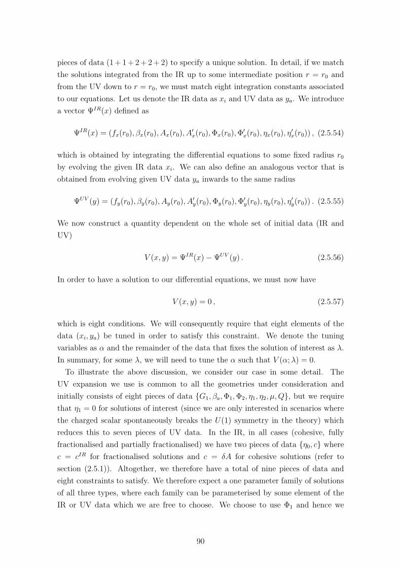
pieces of data (1+ 1+ 2+ 2+2) to specify a unique solution. In detail, if we match

the solutions integrated from the IR up to some intermediate position r = r0 and

from the UV down to r = r0, we must match eight integration constants associated

to our equations. Let us denote the IR data as xi and UV data as ya. We introduce

a vector ΨIR(x) defined as

ΨIR(x) = (fx(r0), βx(r0), Ax(r0), A′x(r0),Φx(r0),Φ

′x(r0), ηx(r0), η

′x(r0)) , (2.5.54)

which is obtained by integrating the differential equations to some fixed radius r0

by evolving the given IR data xi. We can also define an analogous vector that is

obtained from evolving given UV data ya inwards to the same radius

ΨUV (y) = (fy(r0), βy(r0), Ay(r0), A′y(r0),Φy(r0),Φ

′y(r0), ηy(r0), η

′y(r0)) . (2.5.55)

We now construct a quantity dependent on the whole set of initial data (IR and

UV)

V (x, y) = ΨIR(x)−ΨUV (y) . (2.5.56)

In order to have a solution to our differential equations, we must now have

V (x, y) = 0 , (2.5.57)

which is eight conditions. We will consequently require that eight elements of the

data (xi, ya) be tuned in order to satisfy this constraint. We denote the tuning

variables as α and the remainder of the data that fixes the solution of interest as λ.

In summary, for some λ, we will need to tune the α such that V (α;λ) = 0.

To illustrate the above discussion, we consider our case in some detail. The

UV expansion we use is common to all the geometries under consideration and

initially consists of eight pieces of data G1, βa,Φ1,Φ2, η1, η2, µ,Q, but we require

that η1 = 0 for solutions of interest (since we are only interested in scenarios where

the charged scalar spontaneously breaks the U(1) symmetry in the theory) which

reduces this to seven pieces of UV data. In the IR, in all cases (cohesive, fully

fractionalised and partially fractionalised) we have two pieces of data η0, c where

c = cIR for fractionalised solutions and c = δA for cohesive solutions (refer to

section (2.5.1)). Altogether, we therefore have a total of nine pieces of data and

eight constraints to satisfy. We therefore expect a one parameter family of solutions

of all three types, where each family can be parameterised by some element of the

IR or UV data which we are free to choose. We choose to use Φ1 and hence we

90

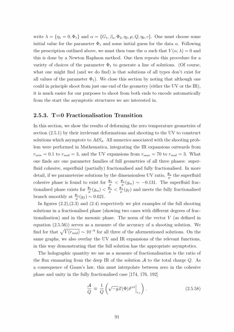
write λ = η1 = 0,Φ1 and α = G1, βa,Φ2, η2, µ,Q, η0, c. One must choose some

initial value for the parameter Φ1 and some initial guess for the data α. Following

the prescription outlined above, we must then tune the α such that V (α;λ) = 0 and

this is done by a Newton Raphson method. One then repeats this procedure for a

variety of choices of the parameter Φ1 to generate a line of solutions. (Of course,

what one might find (and we do find) is that solutions of all types don’t exist for

all values of the parameter Φ1). We close this section by noting that although one

could in principle shoot from just one end of the geometry (either the UV or the IR),

it is much easier for our purposes to shoot from both ends to encode automatically

from the start the asymptotic structures we are interested in.

2.5.3. T=0 Fractionalisation Transition

In this section, we show the results of deforming the zero temperature geometries of

section (2.5.1) by their irrelevant deformations and shooting to the UV to construct

solutions which asymptote to AdS4. All numerics associated with the shooting prob-

lem were performed in Mathematica, integrating the IR expansions outwards from

rmin = 0.1 to rmid = 3, and the UV expansions from rmax = 70 to rmid = 3. What

one finds are one parameter families of full geometries of all three phases: super-

fluid cohesive, superfluid (partially) fractionalised and fully fractionalised. In more

detail, if we parameterise solutions by the dimensionless UV ratio, Φ1

µthe superfluid

cohesive phase is found to exist for Φ1

µ< Φ1

µ(gm) ∼ −0.131. The superfluid frac-

tionalised phase exists for Φ1

µ(gm) <

Φ1

µ< Φ1

µ(gf ) and meets the fully fractionalised

branch smoothly at Φ1

µ(gf ) ∼ 0.621.

In figures (2.2),(2.3) and (2.4) respectively we plot examples of the full shooting

solutions in a fractionalised phase (showing two cases with different degrees of frac-

tionalisation) and in the mesonic phase. The norm of the vector V (as defined in

equation (2.5.56)) serves as a measure of the accuracy of a shooting solution. We

find for that√

V (rmid) ∼ 10−9 for all three of the aformentioned solutions. On the

same graphs, we also overlay the UV and IR expansions of the relevant functions,

in this way demonstrating that the full solution has the appropriate asymptotics.

The holographic quantity we use as a measure of fractionalisation is the ratio of

the flux emanating from the deep IR of the solution A to the total charge Q. As

a consequence of Gauss’s law, this must interpolate between zero in the cohesive

phase and unity in the fully fractionalised case [174, 176, 192]

AQ

≡ 1

Q

(√−gZ(Φ)F rt∣∣∣r+

)

. (2.5.58)

91

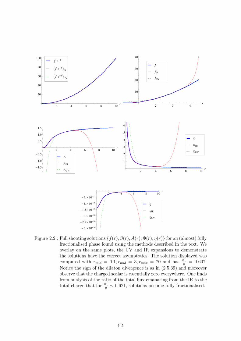
2 4 6 8 10r

20

40

60

80

100

I f e-ΒMUV

I f e-ΒMIR

f e-Β

2 3 4r

10

20

30

40

fUV

fIR

f

2 4 6 8 10r

-1.5

-1.0

-0.5

0.5

1.0

1.5

AUV

AIR

A

2 4 6 8 10r

1

2

3

4

5

6

FUV

FIR

F

2 4 6 8 10r

-3.´10-16

-2.5´10-16

-2.´10-16

-1.5´10-16

-1.´10-16

-5.´10-17

ΗUV

ΗIR

Η

Figure 2.2.: Full shooting solutions f(r), β(r), A(r),Φ(r), η(r) for an (almost) fullyfractionalised phase found using the methods described in the text. Weoverlay on the same plots, the UV and IR expansions to demonstratethe solutions have the correct asymptotics. The solution displayed wascomputed with rmid = 0.1, rmid = 3, rmax = 70 and has Φ1

µ= 0.607.

Notice the sign of the dilaton divergence is as in (2.5.39) and moreoverobserve that the charged scalar is essentially zero everywhere. One findsfrom analysis of the ratio of the total flux emanating from the IR to thetotal charge that for Φ1

µ∼ 0.621, solutions become fully fractionalised.

92

2 4 6 8 10r

20

40

60

80

100

I f e-ΒMUV

I f e-ΒMIR

f e-Β

2 3 4r

10

20

30

40

fUV

fIR

f

2 4 6 8 10r

-1.5

-1.0

-0.5

0.5

1.0

1.5

AUV

AIR

A

2 4 6 8 10r

1

2

3

4

5

6

7

FUV

FIR

F

2 4 6 8 10r

0.05

0.10

0.15

0.20

0.25

0.30

ΗUV

ΗIR

Η

Figure 2.3.: Full shooting solutions f(r), β(r), A(r),Φ(r), η(r) for a partially frac-tionalised phase found using the methods described in the text. Weoverlay on the same plots, the UV and IR expansions to demonstratethe solutions have the correct asymptotics. The solution displayed wascomputed with rmid = 0.1, rmid = 3, rmax = 70 and has Φ1

µ= 0.0964.

Notice the sign of the dilaton divergence is as in (2.5.39) and moreoverobserve that the charged scalar is non-zero. One finds that this partiallyfractionalised phase persists until Φ1

µ∼ −0.131.

93

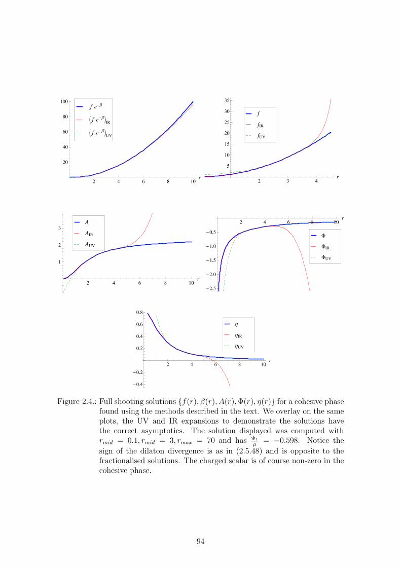
2 4 6 8 10r

20

40

60

80

100

I f e-ΒMUV

I f e-ΒMIR

f e-Β

2 3 4r

5

10

15

20

25

30

35

fUV

fIR

f

2 4 6 8 10r

1

2

3

AUV

AIR

A 2 4 6 8 10r

-2.5

-2.0

-1.5

-1.0

-0.5

FUV

FIR

F

2 4 6 8 10r

-0.4

-0.2

0.2

0.4

0.6

0.8

ΗUV

ΗIR

Η

Figure 2.4.: Full shooting solutions f(r), β(r), A(r),Φ(r), η(r) for a cohesive phasefound using the methods described in the text. We overlay on the sameplots, the UV and IR expansions to demonstrate the solutions havethe correct asymptotics. The solution displayed was computed withrmid = 0.1, rmid = 3, rmax = 70 and has Φ1

µ= −0.598. Notice the

sign of the dilaton divergence is as in (2.5.48) and is opposite to thefractionalised solutions. The charged scalar is of course non-zero in thecohesive phase.

94

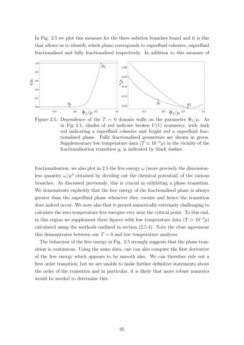
In Fig. 2.5 we plot this measure for the three solution branches found and it is this

that allows us to identify which phase corresponds to superfluid cohesive, superfluid

fractionalised and fully fractionalised respectively. In addition to this measure of

-0.5 0.0 0.5 1.0

0.0

0.2

0.4

0.6

0.8

1.0

-0.5 0.0 0.5 1.0

-0.20

-0.15

-0.10

-0.05

0.00

AQ

ωµ3

Φ1/µΦ1/µ

gc gfgc

gf

Figure 2.5.: Dependence of the T = 0 domain walls on the parameter Φ1/µ. Asin Fig 2.1, shades of red indicate broken U(1) symmetry, with darkred indicating a superfluid cohesive and bright red a superfluid frac-tionalised phase. Fully fractionalised geometries are shown in green.Supplementary low temperature data (T ≃ 10−3µ) in the vicinity of thefractionalisation transition gc is indicated by black dashes.

fractionalisation, we also plot in 2.5 the free energy ω (more precisely the dimension-

less quantity ω/µ3 obtained by dividing out the chemical potential) of the various

branches. As discussed previously, this is crucial in exhibiting a phase transition.

We demonstrate explicitly that the free energy of the fractionalised phase is always

greater than the superfluid phase whenever they coexist and hence the transition

does indeed occur. We note also that it proved numerically extremely challenging to

calculate the zero temperature free energies very near the critical point. To this end,

in this region we supplement these figures with low temperature data (T ≃ 10−3µ)

calculated using the methods outlined in section (2.5.4). Note the close agreement

this demonstrates between our T = 0 and low temperature analyses.

The behaviour of the free energy in Fig. 2.5 strongly suggests that the phase tran-

sition is continuous. Using the same data, one can also compute the first derivative

of the free energy which appears to be smooth also. We can therefore rule out a

first order transition, but we are unable to make further definitive statements about

the order of the transition and in particular, it is likely that more robust numerics

would be needed to determine this.

95

2.5.4. Comments on Finite Temperature

We now make some remarks on fractionalisation at finite temperature. This was

discussed in greater depth in the paper on which this chapter is based [2], but was

not the work of the author of this thesis and thus is not included in detail here.

What was done there was to extrapolate the known finite temperature solutions to

low temperature in order to demonstrate that they connect to the T = 0 geometries

considered in the preceding sections. The analysis reveals some important physics:

the process of lowering the temperature can result in an instability that leads to a

superconducting phase below some critical temperature TC . This critical tempera-

ture is a function of the parameters (data) in the theory and can be dialed to zero

by tuning these parameters beyond certain threshold values. The effect of this is

to produce a structure in phase space under which the theory is superconducting,

known as a ‘superconducting dome’. The position of the edge of this dome was

argued to constrain when T = 0 fractionalisation transitions can occur and in par-

ticular accounts for the absence of a T = 0 fractionalised phase in M-theory as we

shall explain in the next section. The finite temperature analysis is also very illumi-

nating, as through it, one can study various low temperature signatures of quantum

criticality, notably the dynamical critical exponent z and the hyperscaling violation

exponent θ, in terms of which the thermodynamic entropy scales as

S ∼ Td−θz . (2.5.59)

Using equation (2.5.59), it was shown in the aforementioned paper [2] how one

can identify z and θ from numerical fits of the low-temperature analysis. From

these calculations, one sees strikingly the quantum critical nature of the T = 0

fractionalisation transition which leaves a distinctive ‘wedge imprint’ on thermo-

dynamic observables at finite temperature that is characteristic of quantum phase

transitions. Moreover, one can compare the values of θ and z on either side of this

wedge to find that at low temperatures they match extremely closely with the an-

alytic T = 0 values for the cohesive and fractionalised geometries of section (2.5.1),

lending further support for the picture of a T = 0 fractionalisation transition and

verifying the validity of our T = 0 IR geometries. (Further strength for this picture

is also provided by examining the behaviour of the dilaton which is a finite at T 6= 0,

having no divergence but starts to diverge to either plus or minus infinity as the

temperature is lowered, again agreeing with what was found at T = 0).

96

2.6. Class Ib: Bottom - Up Model

Thus far, we have presented a model which falls under class Ia of the classification

introduced through Fig. 2.1. Qualitatively the key point governing its phenomenol-

ogy is the fact that the coupling ZF (Φ) remains finite for an interval of UV scalar

deformations Φ1. It is this fact that allows the model to support a superfluid frac-

tionalised phase (and hence to exhibit a phase transition as these solutions become

thermodynamically preferred).

In this small section, we make a few brief remarks about a model in class Ib.

We consider a theory with the same potential that we have used previously, but

will consider now an even gauge coupling ZF (Φ) = Z20 cosh

(aΦ√3

)

. With this new

coupling, if we have an IR divergent dilaton, then ZF (Φ) must diverge irrespective

of the sign of the dilaton blowup. Qualitatively, we therefore expect the interval

of cohesive solutions exhibited by this theory to be reduced to a single point corre-

sponding to Φ1 = 0. Note that at this point, the solution has Φ(r) = 0 everywhere

and corresponds to an AdS4 to AdS4 charged domain wall.

We conjecture that this model will exhibit a transition from a superfluid cohesive

phase at the point Φ1 = 0, to a superfluid fractionalised phase that persists for some

region 0 < Φ1 < Φ1(gf ), eventually becoming fully fractionalised when Φ1 ≥ Φ1(gf ).

2.7. Class II: M Theory

In this section, we will now discuss a model in class II, which arises as a consistent

truncation of 11D supergravity on an arbitrary Sasaki-Einstein 7-manifold [202, 203].

(Whilst, the details of the compactification and truncation are fascinating we need

not discuss them further here). Structurally, this model shares even gauge coupling

with class Ib, but differs in that it has finite Z everywhere. The equations of motion

of the theory can be obtained from the four dimensional action

SM =1

16πG

∫

d4x√−g

[

R− (1− h2)3/2

1 + 3h2FMNF

MN − 3

2(1− 34|χ|2)2 |Dχ|

2

− 3

2(1− h2)2(∇h)2 − 6

ℓ2(−1 + h2 + |χ|2)

(1− 34|χ|2)2(1− h2)3/2

]

+1

16πG

∫2h(3 + h2)

1 + 3h2F ∧ F .

(2.7.60)

By defining χ = ξeiqϕ and performing the transformation

h = tanh

(Φ√3

)

, ξ =2√3tanh

(η√2

)

, (2.7.61)

97

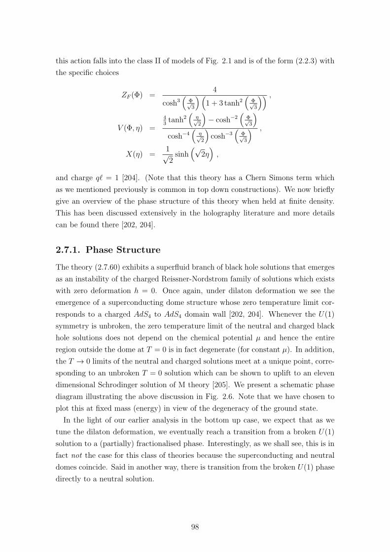
this action falls into the class II of models of Fig. 2.1 and is of the form (2.2.3) with

the specific choices

ZF (Φ) =4

cosh3(

Φ√3

)(

1 + 3 tanh2(

Φ√3

)) ,

V (Φ, η) =

43tanh2

(η√2

)

− cosh−2(

Φ√3

)

cosh−4(

η√2

)

cosh−3(

Φ√3

) ,

X(η) =1√2sinh

(√2η)

,

and charge qℓ = 1 [204]. (Note that this theory has a Chern Simons term which

as we mentioned previously is common in top down constructions). We now briefly

give an overview of the phase structure of this theory when held at finite density.

This has been discussed extensively in the holography literature and more details

can be found there [202, 204].

2.7.1. Phase Structure

The theory (2.7.60) exhibits a superfluid branch of black hole solutions that emerges

as an instability of the charged Reissner-Nordstrom family of solutions which exists

with zero deformation h = 0. Once again, under dilaton deformation we see the

emergence of a superconducting dome structure whose zero temperature limit cor-

responds to a charged AdS4 to AdS4 domain wall [202, 204]. Whenever the U(1)

symmetry is unbroken, the zero temperature limit of the neutral and charged black

hole solutions does not depend on the chemical potential µ and hence the entire

region outside the dome at T = 0 is in fact degenerate (for constant µ). In addition,

the T → 0 limits of the neutral and charged solutions meet at a unique point, corre-

sponding to an unbroken T = 0 solution which can be shown to uplift to an eleven

dimensional Schrodinger solution of M theory [205]. We present a schematic phase

diagram illustrating the above discussion in Fig. 2.6. Note that we have chosen to

plot this at fixed mass (energy) in view of the degeneracy of the ground state.

In the light of our earlier analysis in the bottom up case, we expect that as we

tune the dilaton deformation, we eventually reach a transition from a broken U(1)

solution to a (partially) fractionalised phase. Interestingly, as we shall see, this is in

fact not the case for this class of theories because the superconducting and neutral

domes coincide. Said in another way, there is transition from the broken U(1) phase

directly to a neutral solution.

98

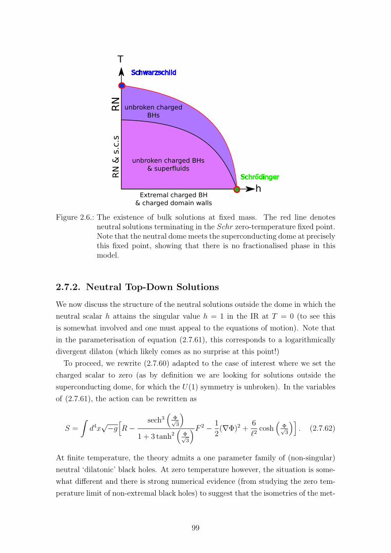
Extremal charged BH& charged domain walls

unbroken charged BHs& superfluids

unbroken chargedBHs

T

h

Schwarzschild

Schrödinger

RNRN

& s.c

.s

Figure 2.6.: The existence of bulk solutions at fixed mass. The red line denotesneutral solutions terminating in the Schr zero-termperature fixed point.Note that the neutral dome meets the superconducting dome at preciselythis fixed point, showing that there is no fractionalised phase in thismodel.

2.7.2. Neutral Top-Down Solutions

We now discuss the structure of the neutral solutions outside the dome in which the

neutral scalar h attains the singular value h = 1 in the IR at T = 0 (to see this

is somewhat involved and one must appeal to the equations of motion). Note that

in the parameterisation of equation (2.7.61), this corresponds to a logarithmically

divergent dilaton (which likely comes as no surprise at this point!)

To proceed, we rewrite (2.7.60) adapted to the case of interest where we set the

charged scalar to zero (as by definition we are looking for solutions outside the

superconducting dome, for which the U(1) symmetry is unbroken). In the variables

of (2.7.61), the action can be rewritten as

S =

∫

d4x√−g

[

R−sech3

(Φ√3

)

1 + 3 tanh2(

Φ√3

)F 2 − 1

2(∇Φ)2 +

6

ℓ2cosh

(Φ√3

)]

. (2.7.62)

At finite temperature, the theory admits a one parameter family of (non-singular)

neutral ‘dilatonic’ black holes. At zero temperature however, the situation is some-

what different and there is strong numerical evidence (from studying the zero tem-

perature limit of non-extremal black holes) to suggest that the isometries of the met-

99

ric are enhanced from the × SO(2) symmetry above to the full SO(1, 2) Lorentz

symmetry [2]. Consequently, and choosing a convenient radial gauge we take,

ds2 =dρ2

F (ρ)+ ρ2sech

(

Φ(ρ)/√3)

ηµνdxµdxν . (2.7.63)

This expression is convenient for the current purposes, but we note that we can

convert it into the form (2.2.10) via

r2 = ρ2 sech(

Φ/√3)

, e−βf = r2 ,√F =

dρ

dr

√

f . (2.7.64)

Singular IR Solutions

We may now proceed to construct the IR solution in question by dimensional re-

duction. First observe that if φ diverges as φ → ∞12 in the IR, then the action

approaches

Ssing =

∫

d4x√−g

[

R− 2e−√3ΦF 2 − 1

2(∇Φ)2 +

3

ℓ2eΦ/

√3]

, (2.7.65)

which can be obtained by reduction of a pure Einstein-Hilbert (with cosmological

constant) action in five dimensions:

S5 =

∫

d5x√

−g[

R +3

ℓ2

]

, (2.7.66)

using a graviphoton ansatz

ds2 = eΦ/√3ds2(M) + e−2Φ/

√3(

dz + 2√2A)2

. (2.7.67)

Under this reduction, pure five-dimensional AdS with metric

ds25 = ℓ25

[dρ2

ρ2+ ρ2

(−dt2 + dx2

)+ ρ2dz2

]

,(ℓ25 = 4ℓ2

), (2.7.68)

reduces to a logarithmic dilaton solution in four dimensions, that is:

ds2 = ℓ25

[dρ2

ρ+ ρ3(−dt2 + dx2)

]

, with Φ = −√3 log(ρ) . (2.7.69)

12The case Φ → −∞ is equivalent by the Φ → −Φ symmetry of the lagrangian coming from 11D.

100

As we now discuss, this solution plays the role of the singular IR we are seeking.

(Note that in this case, the graviphoton field A is trivial, and so we have a standard

circle reduction).

On substituting the metric ansatz (2.7.63) into the equations that follow from

(2.7.65) (with At = µ = constant), one obtains a single, fully decoupled ODE for

the scalar field Φ

ρ2Φ′′(ρ) =−1

2√3tanh

(Φ(ρ)√

3

) [

12− ρ2Φ′(ρ)2(

4 + 3 sech2(

Φ(ρ)√3

))]

−[

1 + 3 sech2(

Φ(ρ)√3

)]

ρΦ′(ρ)

+1

12sech4

(Φ(ρ)√

3

)

ρ3Φ′3(ρ) . (2.7.70)

Note that for any solution, the chemical potential in the boundary theory is arbitrary,

as A is pure gauge in the bulk and if A is to be well-defined, one should choose the

gauge At = 0. The Einstein equations then determine F (ρ) algebraically

F (ρ) =4ℓ−2ρ2 cosh

(Φ/

√3)

4− (ρΦ′/√3)2sech2

(Φ/

√3)− 4ρΦ′/

√3 tanh

(Φ/

√3) , (2.7.71)

where the prime denotes a derivative with respect to the radial direction ρ. The

Φ equation admits an IR expansion, which reproduces (2.7.69) to leading order. It

takes the form

Φ(ρ) = −√3 log ρ+

3√3

2ρ2 + · · · (2.7.72)

and notably has no free parameters. Furthermore, rescaling the ρ coordinate has no

physical effect on the solution. This IR expansion can be integrated directly to the

UV and one finds that it connects to the desired AdS4 solution. Reading off the UV

data, one finds complete agreement with the analytic values corresponding to the

exact solution found in [202]. One can furthermore check that the chemical potential

µ(r∞) − µ(rIR) vanishes. We have therefore demonstrated that the unique neutral

T = 0 solution of (2.7.60) with logarithmically diverging dilaton is the analytic

solution given in Eq (8.2) of [202].

One can also study the approach to zero temperature in further detail. In particu-

lar one observes linear temperature scaling consistent with a z = 2 quantum critical

point. Furthermore, as mentioned briefly above, it can also be demonstrated that

this solution, when lifted to eleven dimensions, is a Schrodinger solution Schr5×KE6

of the full M theory.

101

2.8. Discussion

In summary, we have demonstrated in this chapter how to construct bosonic ana-

logues of so called ‘fractionalisation transitions’ by way of a suitably engineered

bottom-up gravitational action. In addition, we examined the phase diagram of

the M-theory superconductor equipped with these new insights. In particular, we

demonstrate how at zero temperature there is no fractionalisation transition in the

latter case, as one proceeds directly from the broken superfluid cohesive phase to a

neutral phase.

The qualitative structure of the transitions studied in this chapter can be under-

stood by studying the IR behaviour of the dilaton and in particular also the coupling

between the dilaton and the gauge kinetic term. All examples we have encountered

thus far support the conjecture that one cannot have a cohesive phase if the dilaton

coupling to the gauge kinetic term diverges in the infrared (Z → ∞). Physically

this can be explained by observing simply that a diverging Z implies that the effec-

tive gauge coupling vanishes. (This is most easily seen by recalling the form of the

gauge kinetic terms which in a conventional normalisation read ∼ 1e2F 2 and hence

the coupling constant is the reciprocal of the coefficient). Since the electromagnetic

coupling vanishes, matter in the IR cannot source any flux and consequently any

flux there must be sourced by a black hole horizon, resulting in a fractionalised

phase. Note also that our arguments for this behaviour are purely holographic, us-

ing only the properties of the bulk gravitational solutions. Although this physical

reasoning seems rather strong, we know of no rigorous argument that could prove

the aforementioned conjecture. It would also be interesting to understand better

whether one can use bulk arguments to shed light on a possible order parameter for

fractionalisation. This could in principle be rather powerful as one could translate

this into a field theoretic quantity which could then prove useful in entirely different

settings (that could for example be unrelated to holography).

In asymptotically AdS spacetimes, one commonly finds that the near horizon ge-

ometries of zero temperature black holes contain an AdS2 factor, the signature of

which is a diverging critical exponent. It is well known that such geometries have

the rather curious property of finite entropy at zero temperature and consequently

violate the third law of thermodynamics (Nernst’s postulate). Interestingly, how-

ever, they are often unstable when embedded in top-down models and hence the

laws of thermodynamics appear once again to be upheld by the classical solutions

[196, 202, 204]. Note also that although we can often trace finite entropy singulari-

ties at zero temperature to divergent critical exponents, this alone will not necessary

result in singular solution. In particular a divergent critical exponent can be com-

102

pensated for by an equally divergent hyperscaling parameter resulting in a vanishing

entropy at T = 0 [182]. In this manner, one can avoid finite entropy singularities

and this is precisely the mechanism employed by our bottom-up model. In the

M theory case, there is as discussed no fractionalised phase and in particular the

‘would be fractionalised’ Reissner- Nordstrom solutions ultimately end up masked by

a superconducting dome. It could be very interesting to investigate precisely what

conditions must be met for any entropic singularity (i.e. any AdS2 IR geometry) to

be unstable [206] to new phases cloaking it at low temperatures.

103

3. Stationary Elliptic Numerical

Relativity

3.1. Introduction

The Harmonic Einstein equation as introduced in chapter (1.3) is the vacuum Ein-

stein equation together with a gauge fixing term that is taken to be that of DeTurck.

For static black holes that have been analytically continued to Euclidean signature,

this equation was shown in the introduction to be elliptic and hence can be tackled

as an elliptic boundary value problem, where Ricci flow and Newton’s method con-

stitute good numerical algorithms to solve the system. In this chapter, we extend

these results to the stationary case which must be treated in the full Lorentzian

signature as there exists no analytic continuation of a general stationary spacetime

to a smooth, real geometry.

We will begin our discussion by reviewing the approach to construct static so-

lutions using the Harmonic Einstein equation, but this time recasting the analysis

entirely from a Lorentzian perspective, demonstrating that the equation is elliptic.

The key observation to proceed, is that as a consequence of the static symmetries,

the Harmonic Einstein equations give precisely the same equations for the metric

components in either Euclidean or Lorentzian signature (provided that we use co-

ordinates adapted to the static symmetry). Whilst in general then the Lorentzian

Harmonic Einstein equation is hyperbolic, this useful observation shows that when

restricted to static metrics, it is in fact elliptic and can thus be solved as a boundary

value problem. We then proceed to the full stationary case and consider the char-

acter of the general Lorentzian Harmonic Einstein equation. We demonstrate that

for the case of a globally timelike stationary Killing field, the associated equations

are still in fact elliptic and moreover from this analysis it becomes clear that the

threat to ellipticity is physically due to ergo-regions, where the timelike Killing field

becomes spacelike. Since ultimately, we are most interested in the construction of

black holes, we will need to relax the globally timelike restriction. To do this, we

make a Kaluza-Klein ansatz for stationary black holes, motivated by the rigidity

104

theorem [35], that has also been used by Harmark in the classification of higher

dimensional black holes [207]. As a direct consequence of rigidity, Killing symme-

tries in the directions of angular or linear motion of the horizon are assumed and

it turns out that this is crucial in maintaining ellipticity in the presence of ergo-

regions. At this point, based on the analytic treatment of the uniqueness theorems

for stationary problems, we make the assumption that the base manifold is Rieman-

nian and that the horizons and axes of symmetry constitute (physical) boundaries

on this base manifold (we will clarify the meaning of ‘base manifold’ in the next

section). With these conditions, we are able to conclude the Harmonic Einstein

equation restricted to our class of stationary spacetimes is in fact elliptic and we

determine suitable boundary conditions at any horizons and axes in a manner anal-

ogous to the Lorentzian static case. These are shown to be compatible with Ricci

flat (as opposed to soliton) solutions, but unfortunately the maximum principle of

the static case does not readily generalise to stationary geometries. Finally, we end

this chapter by showing how the Kerr solution satisfies the aforementioned boundary

conditions.

3.2. Static Spacetimes from a Lorentzian

Perspective

Instead of immediately studying stationary spacetimes, it will be instructive to first

revisit the static case, this time in Lorentzian signature. That is to say, we will

not perform an analytic continuation in time to arrive at a Riemannian geometry.

The Harmonic Einstein equation, however, is not elliptic for a general Lorentzian

manifold and without ellipticity, as we have discussed now at length, one would

not expect to be able to impose the various boundary conditions that we require

physically in a well posed manner. All is not lost however as we shall now discuss.

Consider a chart away from the horizon which manifests the static symmetry,

ds2 = gµνdxµdxν = −N(x)dt2 + hij(x)dx

idxj , (3.2.1)

so that N > 0. This form of the metric will be very important for the discussion that

follows. We should regard the time coordinate as fibered over a base manifold Mwith Riemannian metric ds2M = hij(x)dx

idxj. Furthermore, if we assume a similar

structure for the reference metric, namely that it is static with respect to ∂/∂t so

105

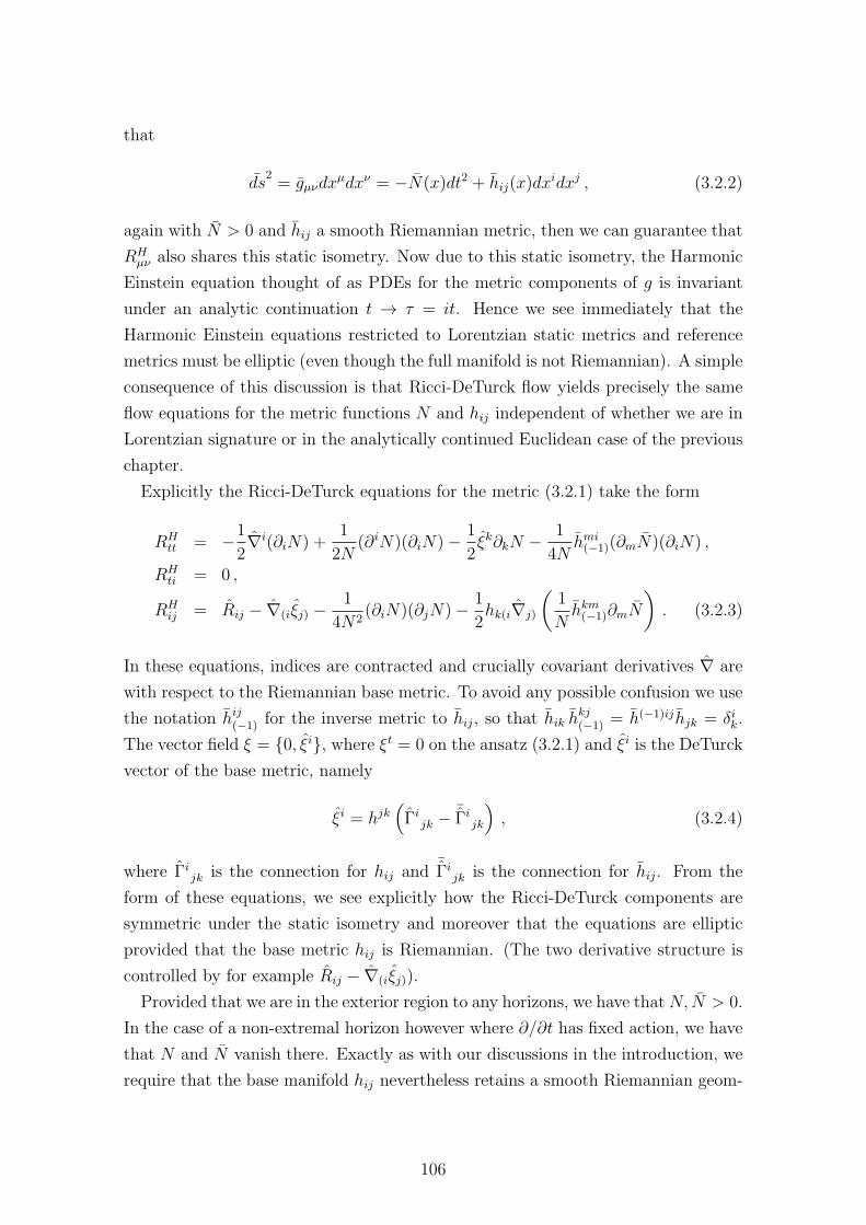
that

ds2= gµνdx

µdxν = −N(x)dt2 + hij(x)dxidxj , (3.2.2)

again with N > 0 and hij a smooth Riemannian metric, then we can guarantee that

RHµν also shares this static isometry. Now due to this static isometry, the Harmonic

Einstein equation thought of as PDEs for the metric components of g is invariant

under an analytic continuation t → τ = it. Hence we see immediately that the

Harmonic Einstein equations restricted to Lorentzian static metrics and reference

metrics must be elliptic (even though the full manifold is not Riemannian). A simple

consequence of this discussion is that Ricci-DeTurck flow yields precisely the same

flow equations for the metric functions N and hij independent of whether we are in

Lorentzian signature or in the analytically continued Euclidean case of the previous

chapter.

Explicitly the Ricci-DeTurck equations for the metric (3.2.1) take the form

RHtt = −1

2∇i(∂iN) +

1

2N(∂iN)(∂iN)− 1

2ξk∂kN − 1

4Nhmi(−1)(∂mN)(∂iN) ,

RHti = 0 ,

RHij = Rij − ∇(iξj) −

1

4N2(∂iN)(∂jN)− 1

2hk(i∇j)

(1

Nhkm(−1)∂mN

)

. (3.2.3)

In these equations, indices are contracted and crucially covariant derivatives ∇ are

with respect to the Riemannian base metric. To avoid any possible confusion we use

the notation hij(−1) for the inverse metric to hij, so that hik hkj(−1) = h(−1)ijhjk = δik.

The vector field ξ = 0, ξi, where ξt = 0 on the ansatz (3.2.1) and ξi is the DeTurck

vector of the base metric, namely

ξi = hjk(

Γijk − ¯

Γijk

)

, (3.2.4)

where Γijk is the connection for hij and

¯Γi

jk is the connection for hij. From the

form of these equations, we see explicitly how the Ricci-DeTurck components are

symmetric under the static isometry and moreover that the equations are elliptic

provided that the base metric hij is Riemannian. (The two derivative structure is

controlled by for example Rij − ∇(iξj)).

Provided that we are in the exterior region to any horizons, we have thatN, N > 0.

In the case of a non-extremal horizon however where ∂/∂t has fixed action, we have

that N and N vanish there. Exactly as with our discussions in the introduction, we

require that the base manifold hij nevertheless retains a smooth Riemannian geom-

106

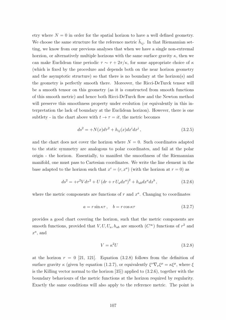
etry where N = 0 in order for the spatial horizon to have a well defined geometry.

We choose the same structure for the reference metric hij. In that Riemannian set-

ting, we know from our previous analyses that when we have a single non-extremal

horzion, or alternatively multiple horizons with the same surface gravity κ, then we

can make Euclidean time periodic τ ∼ τ + 2π/κ, for some appropriate choice of κ

(which is fixed by the procedure and depends both on the near horizon geometry

and the asymptotic structure) so that there is no boundary at the horizon(s) and

the geometry is perfectly smooth there. Moreover, the Ricci-DeTurck tensor will

be a smooth tensor on this geometry (as it is constructed from smooth functions

of this smooth metric) and hence both Ricci-DeTurck flow and the Newton method

will preserve this smoothness property under evolution (or equivalently in this in-

terpretation the lack of boundary at the Euclidean horizon). However, there is one

subtlety - in the chart above with t→ τ = it, the metric becomes

ds2 = +N(x)dτ 2 + hij(x)dxidxj , (3.2.5)

and the chart does not cover the horizon where N = 0. Such coordinates adapted

to the static symmetry are analogous to polar coordinates, and fail at the polar

origin - the horizon. Essentially, to manifest the smoothness of the Riemannian

manifold, one must pass to Cartesian coordinates. We write the line element in the

base adapted to the horizon such that xi = (r, xa) (with the horizon at r = 0) as

ds2 = +r2V dτ 2 + U (dr + r Uadxa)2 + habdx

adxb , (3.2.6)

where the metric components are functions of r and xa. Changing to coordinates

a = r sinκτ , b = r cosκτ (3.2.7)

provides a good chart covering the horizon, such that the metric components are

smooth functions, provided that V, U, Ua, hab are smooth (C∞) functions of r2 and

xa, and

V = κ2U (3.2.8)

at the horizon r = 0 [21, 121]. Equation (3.2.8) follows from the definition of

surface gravity κ (given by equation (1.2.7), or equivalently ξν∇νξµ = κξµ, where ξ

is the Killing vector normal to the horizon [35]) applied to (3.2.6), together with the

boundary behaviours of the metric functions at the horizon required by regularity.

Exactly the same conditions will also apply to the reference metric. The point is

107

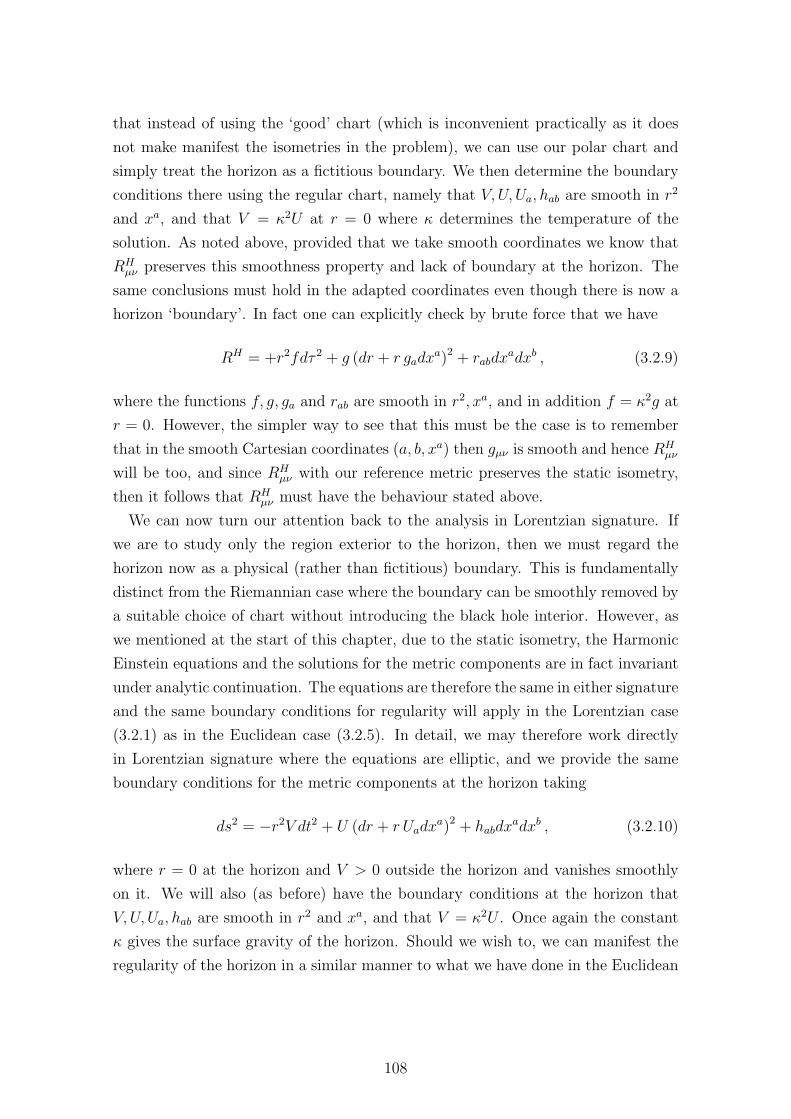
that instead of using the ‘good’ chart (which is inconvenient practically as it does

not make manifest the isometries in the problem), we can use our polar chart and

simply treat the horizon as a fictitious boundary. We then determine the boundary

conditions there using the regular chart, namely that V, U, Ua, hab are smooth in r2

and xa, and that V = κ2U at r = 0 where κ determines the temperature of the

solution. As noted above, provided that we take smooth coordinates we know that

RHµν preserves this smoothness property and lack of boundary at the horizon. The

same conclusions must hold in the adapted coordinates even though there is now a

horizon ‘boundary’. In fact one can explicitly check by brute force that we have

RH = +r2fdτ 2 + g (dr + r gadxa)2 + rabdx

adxb , (3.2.9)

where the functions f, g, ga and rab are smooth in r2, xa, and in addition f = κ2g at

r = 0. However, the simpler way to see that this must be the case is to remember

that in the smooth Cartesian coordinates (a, b, xa) then gµν is smooth and hence RHµν

will be too, and since RHµν with our reference metric preserves the static isometry,

then it follows that RHµν must have the behaviour stated above.

We can now turn our attention back to the analysis in Lorentzian signature. If

we are to study only the region exterior to the horizon, then we must regard the

horizon now as a physical (rather than fictitious) boundary. This is fundamentally

distinct from the Riemannian case where the boundary can be smoothly removed by

a suitable choice of chart without introducing the black hole interior. However, as

we mentioned at the start of this chapter, due to the static isometry, the Harmonic

Einstein equations and the solutions for the metric components are in fact invariant

under analytic continuation. The equations are therefore the same in either signature

and the same boundary conditions for regularity will apply in the Lorentzian case

(3.2.1) as in the Euclidean case (3.2.5). In detail, we may therefore work directly

in Lorentzian signature where the equations are elliptic, and we provide the same

boundary conditions for the metric components at the horizon taking

ds2 = −r2V dt2 + U (dr + r Uadxa)2 + habdx

adxb , (3.2.10)

where r = 0 at the horizon and V > 0 outside the horizon and vanishes smoothly

on it. We will also (as before) have the boundary conditions at the horizon that

V, U, Ua, hab are smooth in r2 and xa, and that V = κ2U . Once again the constant

κ gives the surface gravity of the horizon. Should we wish to, we can manifest the

regularity of the horizon in a similar manner to what we have done in the Euclidean

108

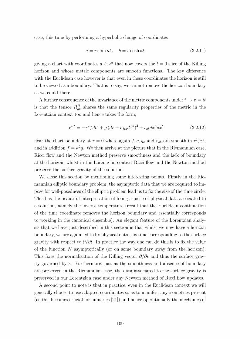
case, this time by performing a hyperbolic change of coordinates

a = r sinhκt , b = r coshκt , (3.2.11)

giving a chart with coordinates a, b, xa that now covers the t = 0 slice of the Killing

horizon and whose metric components are smooth functions. The key difference

with the Euclidean case however is that even in these coordinates the horizon is still

to be viewed as a boundary. That is to say, we cannot remove the horizon boundary

as we could there.

A further consequence of the invariance of the metric components under t→ τ = it

is that the tensor RHµν shares the same regularity properties of the metric in the

Lorentzian context too and hence takes the form,

RH = −r2fdt2 + g (dr + r gadxa)2 + rabdx

adxb (3.2.12)

near the chart boundary at r = 0 where again f, g, ga and rab are smooth in r2, xa,

and in addition f = κ2g. We then arrive at the picture that in the Riemannian case,

Ricci flow and the Newton method preserve smoothness and the lack of boundary

at the horizon, whilst in the Lorentzian context Ricci flow and the Newton method

preserve the surface gravity of the solution.

We close this section by mentioning some interesting points. Firstly in the Rie-

mannian elliptic boundary problem, the asymptotic data that we are required to im-

pose for well-posedness of the elliptic problem lead us to fix the size of the time circle.

This has the beautiful interpretation of fixing a piece of physical data associated to

a solution, namely the inverse temperature (recall that the Euclidean continuation

of the time coordinate removes the horizon boundary and essentially corresponds

to working in the canonical ensemble). An elegant feature of the Lorentzian analy-

sis that we have just described in this section is that whilst we now have a horizon

boundary, we are again led to fix physical data this time corresponding to the surface

gravity with respect to ∂/∂t. In practice the way one can do this is to fix the value

of the function N asymptotically (or on some boundary away from the horizon).

This fixes the normalisation of the Killing vector ∂/∂t and thus the surface grav-

ity governed by κ. Furthermore, just as the smoothness and absence of boundary

are preserved in the Riemannian case, the data associated to the surface gravity is

preserved in our Lorentzian case under any Newton method of Ricci flow updates.

A second point to note is that in practice, even in the Euclidean context we will

generally choose to use adapted coordinates so as to manifest any isometries present

(as this becomes crucial for numerics [21]) and hence operationally the mechanics of

109

solving this static problem are in fact exactly the same in either signature. For the

purposes of implementation, whether regularity is imposed at a ‘real’ or fictitious

boundary where some set of coordinates degenerates is of no consequence. That

said, it turns out that there is in fact one important advantage that one gains by

thinking about even the purely static problem in a Lorentzian signature, namely

that in this case one is able to consider multiple Killing horizons with respect to

∂/∂t with different associated surface gravities, each of which is separately preserved

by the Newton method/Ricci flow. We could not consider such situations in a purely

Euclidean framework of course as we may only use analytic continuation to remove

a single horizon boundary, and in the process of doing so, any remaining horizons

become conical singularities.

Having revisited the framework of static elliptic numerical relativity in Lorentzian

signature, we now turn to a discussion of stationary solutions where no Riemannian

description is possible and we will be required to treat the problem in Lorentzian

signature from the outset.

3.3. Stationary Spacetimes with Globally

Timelike Killing Vector

We now wish to use the methods above to find stationary vacuum solutions. In

this section, we will begin this task by studying the case of stationary solutions

with a globally timelike Killing vector and will show that the associated Harmonic

Einstein equation is elliptic. Consequently all our techniques from the static case

will carry over with only small modification. Whilst a good first step, this situation

corresponds physically to a scenario where there are no horizons or ergo-regions

present in the spacetime. Since ultimately we wish to construct stationary black

holes, in subsequent sections we will need to discuss how to relax the requirement

of a globally timelike Killing field.

Consider the most general stationary metric with Killing vector T = ∂/∂t, which

we may write using coordinates adapted to the stationary isometry as

g = −N(x)(dt+ Ai(x)dx

i)2

+ hij(x)dxidxj. (3.3.13)

Under our starting assumption that T is a globally timelike vector field, we have that

N > 0 everywhere and we may furthermore assume that N is bounded. Physically,

as alluded to above this means that our spacetime has no Killing horizons and

moreover no ergo-region. One may calculate that det gµν = −N dethij and we then

110

see that provided the metric g is Lorentzian and smooth, so that det gµν < 0 and

bounded, we have that the base dethij > 0. We then have the useful result that we

may regard the metric (3.3.13) as a smooth fibration of time over a base manifold

M, so that (M, h) is a smooth Riemanian manifold with Euclidean signature metric

hij.

It is interesting to note that whilst one might imagine that for a stationary space-

time, the natural way to think of the metric would be through the ADM ansatz,

(3.3.13) is in fact not of this form. Rather, it is a Kaluza-Klein ansatz where we

have reduced over the time direction. Consequently the base manifold (M, h) is not

the submanifold obtained by taking a constant t slice of the full geometry. We can

now put all of this together to show that

RHµν ∼ −1

2gαβ∂α∂βgµν + . . . = −1

2hij∂i∂jgµν + . . . (3.3.14)

where as usual . . . denote terms with less than two derivatives. Critically, despite

the fact that gµν is Lorentzian, since the metric components have no t dependence,

the character of the two derivative terms is governed entirely by the Euclidean

metric hij. (In arriving at this conclusion, we have implicitly used the fact that for

the metric (3.3.13), gij = hij which is a well-known property of the Kaluza-Klein

ansatz). This immediately implies that the Harmonic Einstein equations are elliptic

and hence this stationary problem reduces to an elliptic problem on the Riemannian

base manifold M.

It is also very important that RHµν is itself a tensor that is symmetric with respect

to the stationary isometry. This is an important constraint as without this, Ricci-

DeTurck flow and the Newton method will not consistently truncate to the class

of stationary metrics. Said in another way, without this, under Ricci flow/Newton

method updates a metric which is initially stationary would not in general remain

stationary (preserve the stationary symmetries). In order that RHµν preserves the

stationary isometries we will require that the reference metric g is also a smooth

Lorentzian metric which is itself stationary with respect to the vector field T , so

that

g = −N(x)(dt+ Ai(x)dx

i)2

+ hij(x)dxidxj , (3.3.15)

where we also assume here that T is globally timelike and bounded with respect to

g so that N > 0 and bounded. Then hij gives a second Riemannian metric on the

same manifold M. Since RHµν preserves the stationary symmetry, the Ricci-DeTurck

flow can be consistently truncated to a parabolic flow on the space of Lorentzian

111

stationary metrics. Since this flow remains diffeomorphic to Ricci flow (subject at

least to the normal component of ξ vanishing on any boundaries), we arrive at the

interesting result that we may apply Ricci flow to Lorentzian stationary spacetimes.

Likewise the Newton method will preserve the symmetry.

To summarise then, this section contains the key ideas and techniques that underly

our whole approach to recasting the stationary case as an elliptic problem. The

procedure is straightforward - one writes the metric in Kaluka-Klein form (3.3.13)

whereupon it becomes clear that the character of the equations is then governed

by the base metric hij. By proving that this metric is Riemannian, one may then

prove ellipticity of the equations. To do this one needs to make assumptions about

the nature of the spacetime under study. In a situation where the solution we

wish to find has a stationary Killing vector that is globally timelike and bounded

then nearby to that solution, hij is Riemannian and the character of the Harmonic

Einstein equation will be elliptic. Subject to imposing suitable (elliptic) boundary

conditions on any boundaries/asymptotic regions, we may use the Lorentzian Ricci-

DeTurck flow or Newton method to solve for the solution in essentially the same

manner as in the static case1.

There is however one very important caveat compared with the static case which

is worth mentioning. Whilst there, we had the vacuum maximum principle of [121]

which subject to suitable boundary conditions was able to rule out the existence of

soliton solutions, we do not know of how to prove an analogous result in this new

stationary setting. The essence of the problem is easy to see. Whilst in the (vacuum)

static case, we had the inequality ∇2φ + ξµ∂µφ = 2∇µξν∇µξν > 0, where φ = |ξ|2,in the stationary case, this inequality does not appear to hold since in Lorentzian

signature, with only stationary symmetry, ∇µξν∇µξν is of indefinite sign. It is

unclear therefore how to formulate a maximum principle for the stationary case

1For completeness we include here a discussion of boundary conditions in the case of ‘finite’ (i.e.not necessarily asymptotic) boundary. We recall that for a solution to the Harmonic Einsteinequation to be Ricci flat we require that ξ = 0. Whatever boundary conditions we choose musttherefore compatible with vanishing ξ. Let us briefly consider the case of Dirichlet conditionsand consider taking adapted coordinates to the boundary so that we have

ds2 = −N(x) (dt+Ar(x)dr +Aa(x)dxa)

2+ V dr2 + Vadrdx

a + hab(x)dxadxb ,

(3.3.16)

where xi = (r, xa) and the boundary is at r = 0. Fixing the induced metric specifies Dirichletconditions for N , Aa and hab. Requiring that ξt, ξr and ξa vanish then provides conditions forV , Va, and Ar. We have hence fixed all the metric components on the boundary. (Naively thismight seem like ‘too much data’ but of course the key point here is that we are also imposingξ = 0). For the reasons outlined above and presented in [121], we expect that this will constitutea well-posed elliptic boundary value problem. Then, subject to imposing suitable conditions atany other boundaries in the problem (e.g. asymptotically) that are consistent with vanishingξ, we can hope to obtain solutions with globally vanishing DeTurck vector as desired.

112

(the proof certainly doesn’t seem to proceed in the same relatively straightforward

manner as before). In principle there could therefore be soliton solutions even when

we have boundary conditions compatible with vanishing ξ. In practice, as alluded

to before, this rarely presents problems and what one has to do is simply test a

solution that is found to see whether is a true Ricci flat solution or a soliton. (The

only scenarios we can envision where this could be a problem would be when one is

looking for a particular Ricci flat solution amidst a whole slew of solitons, but aside

from these situations the pragmatic approach will suffice).

For completeness and to close this section we now explicitly show the stationary

Ricci-DeTurck flow equations (which give the Harmonic Einstein equations at a fixed

point ∂/∂λ = 0). These are the equations which one has to solve numerically to

find a solution. The key point to notice, pertaining to our earlier discussions is the

two derivative structure, indicated by way of an over-brace:

∂N

∂λ=

=hkm∂k∂mN+...︷ ︸︸ ︷

∇i(∂iN) − 1

N(∂iN)(∂iN)− N2

2F ijFij + ξk∂kN

+1

2Nhkm(−1)(∂mN)(∂kN) + hkm(−1)N(Ai − Ai)Fjm∂kN

+1

2(Ai − Ai)

2hkm(−1)(∂mN)(∂kN) ,

∂Ai

∂λ=

=hkm∂k∂mAi+...︷ ︸︸ ︷

∇kFik + ∇i(Akξk) + ∇i(∇pAp − ¯∇pAp)−

1

NFij∂

jN

+ ξkFki +1

2Nhkm(−1)Fki∂mN − hkm(−1)N(Aj − Aj)FikFjm

+1

2hkm(−1)(Ap − Ap)

2Fki∂mN

+ ∇i

((1

2Nhmp(−1)(Am − Am)

+1

N(Ap − Ap) +

1

2hkp(−1)(Am − Am)2(Ak − Ak)

)

∂pN

)

+ ∇i(hkm(−1)N(Aj − Aj)(Ak − Ak)Fjm) ,

∂hij∂λ

=

=hkm∂k∂mhij+...︷ ︸︸ ︷

−2Rij + 2∇(iξj)+1

2N2(∂iN)(∂jN)−NF k

j Fki

(1

2hik∇j(

1

Nhkm(−1)∂mN) + hik∇j(h

km(−1)N Fqm(Aq − Aq))

+1

2hik∇j(h

km(−1)(A

p − Ap)2∂mN) + (i ↔ j)

)

.

(3.3.17)

113

In the above, indices are contracted and covariant derivatives ∇ are with respect to

the base metric hij, and we have defined the antisymmetric tensors Fij ≡ ∂iAj−∂jAi

and Fij ≡ ∂iAj − ∂jAi in a manner analogous to electrodynamics. Again ξi is the

DeTurck vector of the base metric defined as before in (3.2.4).

We note also that the individual components of the DeTurck tensor RHµν may be

derived from the above equations using the fact that

∂N

∂λ= −2RH

tt ,

∂Ai

∂λ= − 2

N(RH

it −RHttAi) ,

∂hij∂λ

= −2(RHij +RH

ttAiAj −RHitAj −RH

jtAi) . (3.3.18)

3.4. Stationary Black Holes

We are now in a position to consider the case of Ricci flat, non-extremal stationary

black holes. In this situation, in contrast to the discussion above, the norm of T

will vanish either at the horizon itself (if T is a globally timelike vector, such as

for certain Kerr-AdS black holes [208]), or alternatively outside the horizon at the

boundary of an ergo-region. Since we are (at least for now) interested only in the

region outside the horizon, in the first of these cases, we may treat the system as for

globally timelike T , with the horizon regarded as a boundary of the base manifold

M where suitable data is to be imposed. In the latter more general case however,

outside the horizon but within the ergo-region we will have that the norm of T > 0,

and hence dethij < 0. Our arguments in the previous section will then require

modification as the base manifold fails to be Riemannian.

In order to make progress here we will need to make use of the so called Rigidity

Theorem for stationary black holes, proved in D > 4 by Ishibashi, Hollands and

Wald [54] and by Moncrief and Isenberg [209] for various asymptotics including

asymptotic flatness. This theorem states that given a stationary Killing vector T ,

and a rotating non-extremal Killing horizon with topology ×Σ, (for Σ compact),

there exists a Killing vector K that commutes with T , and is normal to the horizon.

Note that of course the stationary Killing vector T will not be normal to the horizon

in the presence of rotation. Moreover, there also exist some further number N ≥ 1

of commuting Killing vectors Ra, which also commute with T and generate closed

orbits with period 2π so that K may be written in terms of these as

K = T + ΩaRa (3.4.19)

114

for some constants Ωa. What this means is that rotation of the horizon is generated

by an isometry of the spacetime. The horizon moves rigidly with respect to the orbits

of K in its exterior and hence with respect to the asymptotic rotation generators

Ra. If this were not the the case, then one could argue on physical grounds that we

should see gravitational radiation emitted from a region near the horizon, ultimately

violating the assumption of stationarity.

Motivated by the Rigidity Theorem, we will assume that our stationary spacetime

with Killing vector T has in addition a further N ‘rotational’ Killing vectors Ra for

a = 1, 2, . . . , N . The Ra commute amongst themselves and with the stationary

Killing field T and physically should be thought of as the generators of rotational or

translational isometries. (In the former case, they generate closed orbits with some

fixed period, whilst in the latter case the associated orbits are non-compact). In the

interest of generality, let us assume that there are a number of disconnected horizon

components, H1, . . . ,Hk. The Rigidity Theorem then tells us that each component

is separately a Killing horizon with as associated Killing vector that is given by

some linear combination of the stationary and rotational Killing vectors. We write

this in the form KHm= T + Ωa

HmRa for some constants Ωa

Hm, which we stress may

be different for each component. (Physically one should think of these constants as

corresponding to the angular velocity of the associated Killing horizon).

In view of these assumptions, let us now consider a new metric ansatz using

coordinates adapted to the isometries yA = t, ya, so that

ds2 = gµνdXµdXν = GAB(x)

(dyA + AA

i (x)dxi) (dyB + AB

j (x)dxj)+ hij(x)dx

idxj

(3.4.20)

where T = ∂/∂t and Ra = ∂/∂ya. (Note physically, this metric describes rotation or

linear motion in a Killing direction). Just as with the case of a stationary solution

with globally timelike Killing vector, this new geometry is best thought of as a

fibration of the Killing vector directions over a base manifold M with associated

metric hij. As we shall see, it is once again this base metric which controls the

character of the associated equations. The base manifold M is mathematically the

orbit space of the full Lorentzian manifold with respect to T and Ra. In particular,

if Ra generates a compact orbit, then we can normalise the period to be 2π and

hence the coordinate ya will be periodic as ya ∼ ya + 2π. Note also as before that

the metric hij is not induced on a constant y hypersurface as once again (3.4.20) is

of the Kaluza-Klein form.

Our full spacetime is Lorentzian and thus exterior to any horizons we must have

115

(regardless of ergo-regions) det gµν = detGAB dethij < 0. On any physical bound-

aries or asymptotic regions we have that T is timelike, the Ra are spacelike and

hence the fiber metric GAB is Lorentzian there and the base metric is consequently

Euclidean. On the other hand at a Killing horizon Hm, by definition the norm of

KHm= T+Ωa

HmRa vanishes, and hence detGAB = 0. Similarly, at axes of symmetry

associated to the fixed action of the rotatational Killing vectors Ra we will also have

that detGAB = 0.

In other to make further progress we will now need to make one final assumption.

We emphasise that here what we are really trying to do is to find a useful constructive

numerical technique for finding black hole solutions, as opposed to proving general

results and theorems. Therefore, motivated by the uniqueness theorem treatment of

D = 4 black holes as an elliptic boundary value problem on a Riemannian base (see

for instance [53] and the D dimensional generalisations [106, 107]), we will simply

make the following assumption:

Assumption: (M, h) is a smooth Riemannian manifold with boundaries given

by the horizons and axes of symmetry of the Ra that generate rotational isometries.

A consequence of dethij > 0 everywhere on M, including in particular on the

horizon and axis boundaries is that detGAB ≤ 0 everywhere onM, with it vanishing

only at the horizon or axis boundaries of M. (Note in particular that det gµν = 0

there as one should have anticipated by virtue of the fact that the coordinates of

(3.4.20) break down there). It is of interest to note also that the same ingredients

of relevance in our analysis, namely the structure of the base M, together with the

data associated with the Killing horizon boundaries ΩaHm

and specification of which

Ra vanish at the axis boundaries has been conjectured to provide at least a partial

classification of higher dimensional black holes in terms of their rod structure [207].

3.4.1. Ellipticity of the Harmonic Einstein Equation

In the above analysis it is important to stress that we have not assumed that the

stationary Killing field T is timelike and indeed it is not. In the presence of horizons,

it will become null and in an ergoregion it will become spacelike. Indeed as shown

in (3.4), it was precisely when T failed to be timelike that ellipticity broke down as

the base metric then failed to be Riemannian. Equipped now with our assumption

above on the base metric, the crucial observation we make is that for the class of

116

stationary solutions (3.4.20) we have

RHAB = −1

2gαβ∂α∂βgAB + . . . = −1

2hmn∂m∂nGAB + . . . ,

RHij = −1

2gαβ∂α∂βgµν + . . . = −1

2hmn∂m∂nhij + . . . , (3.4.21)

where again the ellipses represent terms with less than two derivatives. We hence

see explicitly that the equations have character determined solely by the metric hij,

and since M is Riemannian (by assumption), these are elliptic.

In analogy with the previous section, we should also ensure that RHµν shares the

same isometries as the metric (3.4.20) so that we correctly truncate to this class of

stationary solutions under Ricci Flow/Newton method updates. Consequently we

choose for the reference metric

ds2 = gµνdXµdXν = GAB(x)

(dyA + AA

i (x)dxi) (dyB + AB

j (x)dxj)+ hij(x)dx

idxj

(3.4.22)

where T,Ra are again Killing with respect to it and we furthermore assume that

(M, h) is a smooth Riemannian manifold. (Since we are free to choose the reference

metric, which is then fixed, this does not truly impose any further restrictions on

our method).

The final matter to address is boundary conditions. In addition to the asymptotic

boundary, all horizons and axes of symmetry constitute real physical boundaries and

we will need to impose data there. We will discuss this in detail in the next section.

The picture is then that using Ricci-DeTurck flow or the Newton method and be-

ginning with initial data in our stationary class, for small flow times (at least) we

expect to remain in this class and importantly the base (M, h) remains Riemannian.

Subject to choosing suitable initial conditions and provided the aforementioned con-

dition is not violated we should then be able to use this method to find a stationary

black hole.

As in the last section, we now explicitly write down the flow equations that would

need to be solved to carry out such a task. The components of the Harmonic Einstein

equation may be also deduced from these, using the equations

∂GAB

∂λ= −2RH

AB ,

∂ACj

∂λ= −2GAC(RH

jA −RHABA

Bj ) ,

∂hij∂λ

= −2(RHij +RH

ABAAi A

Bj −RH

iAAAj −RH

jAAAi ) . (3.4.23)

117

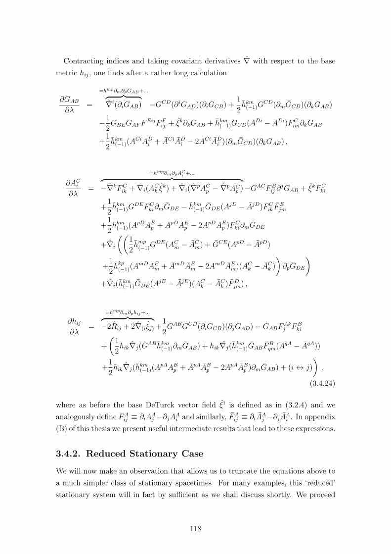
Contracting indices and taking covariant derivatives ∇ with respect to the base

metric hij, one finds after a rather long calculation

∂GAB

∂λ=

=hmp∂m∂pGAB+...︷ ︸︸ ︷

∇i(∂iGAB) −GCD(∂iGAD)(∂iGCB) +1

2hkm(−1)G

CD(∂mGCD)(∂kGAB)

−1

2GBEGAFF

EijF Fij + ξk∂kGAB + hkm(−1)GCD(A

Di − ADi)FCim∂kGAB

+1

2hkm(−1)(A

CiADi + ACiAD

i − 2ACiADi )(∂mGCD)(∂kGAB) ,

∂ACi

∂λ=

=hmp∂m∂pACi +...

︷ ︸︸ ︷

−∇kFCik + ∇i(A

Ck ξ

k) + ∇i(∇pACp − ¯∇pAC

p )−GACFBij ∂

jGAB + ξkFCki

+1

2hkm(−1)G

DEFCki∂mGDE − hkm(−1)GDE(A

jD − AjD)FCik F

Ejm

+1

2hkm(−1)(A

pDAEp + ApDAE

p − 2ApDAEp )F

Cki∂mGDE

+∇i

((1

2hmp(−1)G

DE(ACm − AC

m) + GCE(ApD − ApD)

+1

2hkp(−1)(A

mDAEm + AmDAE

m − 2AmDAEm)(A

Ck − AC

k )

)

∂pGDE

)

+∇i(hkm(−1)GDE(A

jE − AjE)(ACk − AC

k )FDjm) ,

∂hij∂λ

=

=hmp∂m∂phij+...︷ ︸︸ ︷

−2Rij + 2∇(iξj) +1

2GABGCD(∂iGCB)(∂jGAD)−GABF

Akj FB

ki

+

(1

2hik∇j(G

ABhkm(−1)∂mGAB) + hik∇j(hkm(−1)GABF

Bqm(A

qA − AqA))

+1

2hik∇j(h

km(−1)(A

pAABp + ApAAB

p − 2ApAABp )∂mGAB) + (i↔ j)

)

,

(3.4.24)

where as before the base DeTurck vector field ξi is defined as in (3.2.4) and we

analogously define FAij ≡ ∂iA

Aj −∂jAA

i and similarly, FAij ≡ ∂iA

Aj −∂jAA

i . In appendix

(B) of this thesis we present useful intermediate results that lead to these expressions.

3.4.2. Reduced Stationary Case

We will now make an observation that allows us to truncate the equations above to

a much simpler class of stationary spacetimes. For many examples, this ‘reduced’

stationary system will in fact by sufficient as we shall discuss shortly. We proceed

118

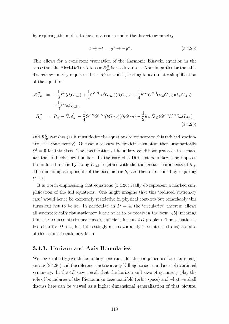
by requiring the metric to have invariance under the discrete symmetry

t→ −t , ya → −ya . (3.4.25)

This allows for a consistent truncation of the Harmonic Einstein equation in the

sense that the Ricci-DeTurck tensor RHµν is also invariant. Note in particular that this

discrete symmetry requires all the AAi to vanish, leading to a dramatic simplification

of the equations

RHAB = −1

2∇i(∂iGAB) +

1

2GCD(∂iGAD)(∂iGCB)−

1

4hkmGCD(∂mGCD)(∂kGAB)

−1

2ξk∂kGAB ,

RHij = Rij − ∇(iξj) −

1

4GABGCD(∂iGCB)(∂jGAD)−

1

2hk(i∇j)(G

ABhkm∂mGAB) ,

(3.4.26)

and RHAi vanishes (as it must do for the equations to truncate to this reduced station-

ary class consistently). One can also show by explicit calculation that automatically

ξA = 0 for this class. The specification of boundary conditions proceeds in a man-

ner that is likely now familiar. In the case of a Dirichlet boundary, one imposes

the induced metric by fixing GAB together with the tangential components of hij.

The remaining components of the base metric hij are then determined by requiring

ξi = 0.

It is worth emphasising that equations (3.4.26) really do represent a marked sim-

plification of the full equations. One might imagine that this ‘reduced stationary

case’ would hence be extremely restrictive in physical contexts but remarkably this

turns out not to be so. In particular, in D = 4, the ‘circularity’ theorem allows

all asymptotically flat stationary black holes to be recast in the form [35], meaning

that the reduced stationary class is sufficient for any 4D problem. The situation is

less clear for D > 4, but interestingly all known analytic solutions (to us) are also

of this reduced stationary form.

3.4.3. Horizon and Axis Boundaries

We now explicitly give the boundary conditions for the components of our stationary

ansatz (3.4.20) and the reference metric at any Killing horizons and axes of rotational

symmetry. In the 4D case, recall that the horizon and axes of symmetry play the

role of boundaries of the Riemannian base manifold (orbit space) and what we shall

discuss here can be viewed as a higher dimensional generalisation of that picture.

119

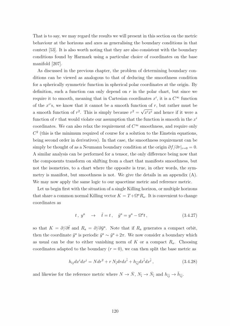
That is to say, we may regard the results we will present in this section on the metric

behaviour at the horizons and axes as generalising the boundary conditions in that

context [53]. It is also worth noting that they are also consistent with the boundary

conditions found by Harmark using a particular choice of coordinates on the base

manifold [207].

As discussed in the previous chapter, the problem of determining boundary con-

ditions can be viewed as analogous to that of deducing the smoothness condition

for a spherically symmetric function in spherical polar coordinates at the origin. By

definition, such a function can only depend on r in the polar chart, but since we

require it to smooth, meaning that in Cartesian coordinates xi, it is a C∞ function

of the xi’s, we know that it cannot be a smooth function of r, but rather must be

a smooth function of r2. This is simply because r2 =√xixi and hence if it were a

function of r that would violate our assumption that the function is smooth in the xi

coordinates. We can also relax the requirement of C∞ smoothness, and require only

C2 (this is the minimum required of course for a solution to the Einstein equations,

being second order in derivatives). In that case, the smoothness requirement can be

simply be thought of as a Neumann boundary condition at the origin ∂f/∂r|r=0 = 0.

A similar analysis can be performed for a tensor, the only difference being now that

the components transform on shifting from a chart that manifests smoothness, but

not the isometries, to a chart where the opposite is true, in other words, the sym-

metry is manifest, but smoothness is not. We give the details in an appendix (A).

We may now apply the same logic to our spacetime metric and reference metric.

Let us begin first with the situation of a single Killing horizon, or multiple horizons

that share a common normal Killing vectorK = T+ΩaRa. It is convenient to change

coordinates as

t , ya → t = t , ya = ya − Ωat , (3.4.27)

so that K = ∂/∂t and Ra = ∂/∂ya. Note that if Ra generates a compact orbit,

then the coordinate ya is periodic ya ∼ ya+2π. We now consider a boundary which

as usual can be due to either vanishing norm of K or a compact Ra. Choosing

coordinates adapted to the boundary (r = 0), we can then split the base metric as

hijdxidxj = Ndr2 + r Nidrdx

i + hijdxidxj , (3.4.28)

and likewise for the reference metric where N → N , Ni → Ni and hij → hij.

120

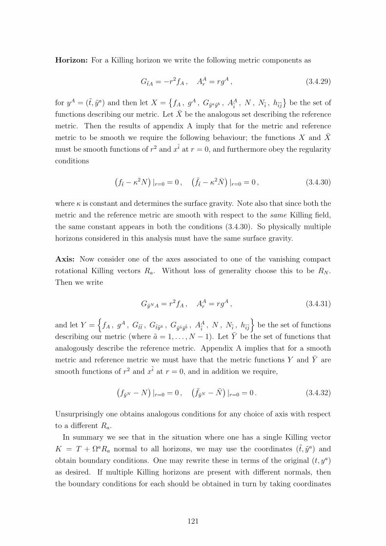
Horizon: For a Killing horizon we write the following metric components as

GtA = −r2fA , AAr = rgA , (3.4.29)

for yA = (t, ya) and then let X =fA , g

A , Gyayb , AAi, N , Ni , hij

be the set of

functions describing our metric. Let X be the analogous set describing the reference

metric. Then the results of appendix A imply that for the metric and reference

metric to be smooth we require the following behaviour; the functions X and X

must be smooth functions of r2 and xi at r = 0, and furthermore obey the regularity

conditions

(ft − κ2N

)|r=0 = 0 ,

(ft − κ2N

)|r=0 = 0 , (3.4.30)

where κ is constant and determines the surface gravity. Note also that since both the

metric and the reference metric are smooth with respect to the same Killing field,

the same constant appears in both the conditions (3.4.30). So physically multiple

horizons considered in this analysis must have the same surface gravity.

Axis: Now consider one of the axes associated to one of the vanishing compact

rotational Killing vectors Ra. Without loss of generality choose this to be RN .

Then we write

GyNA = r2fA , AAr = rgA , (3.4.31)

and let Y =

fA , gA , Gtt , Gtya , Gyayb , A

Ai, N , Ni , hij

be the set of functions

describing our metric (where a = 1, . . . , N − 1). Let Y be the set of functions that

analogously describe the reference metric. Appendix A implies that for a smooth

metric and reference metric we must have that the metric functions Y and Y are

smooth functions of r2 and xi at r = 0, and in addition we require,

(fyN −N

)|r=0 = 0 ,

(fyN − N

)|r=0 = 0 . (3.4.32)

Unsurprisingly one obtains analogous conditions for any choice of axis with respect

to a different Ra.

In summary we see that in the situation where one has a single Killing vector

K = T + ΩaRa normal to all horizons, we may use the coordinates (t, ya) and

obtain boundary conditions. One may rewrite these in terms of the original (t, ya)

as desired. If multiple Killing horizons are present with different normals, then

the boundary conditions for each should be obtained in turn by taking coordinates

121

as in (3.4.27) with Ωa appropriate to each horizon. To complete our discussion

of boundary conditions we note that one should also ensure consistency in regions

where a horizon and axis of symmetry intersect.

A horizon meeting an axis: It is possible to check that the boundary conditions

at the intersection point between a horizon with an axis, or two axes are compatible

with each other by a brute force calculation. We outline this for the case of a metric

intersecting the axis RN , noting that similar results would be found in the other

cases and that the calculation proceeds in a similar manner. We take coordinates

on the base such that the horizon lies at r = 0 and the axis is at θ = 0. In detail,

we have

hijdxidxj = Ndr2 +Mdθ2 + rθAdrdθ + r Bidrdx

i + θ Cidθdxi + hijdx

idxj ,

(3.4.33)

where now i = 1, . . . , D − 3. Then writing,

Gtt = −r2f , Gtya = r2fa , GyN yN = θ2g , GyN ya = θ2ga , GtyN = r2θ2k ,

AAr = r pA , AA

θ = r qA , (3.4.34)

our arguments from appendix A applied to the horizon r = 0 and to the axis θ = 0

then imply that the set of functions characterising the metric found in the equa-

tions (3.4.33) and (3.4.34) above, N,M, . . . , k, pA, qA, together with the remaining

components Gyayb and AAi, must all be smooth functions in r2, θ2 and xi near the

meeting point r = θ = 0. Furthermore regularity requires

(f − κ2N

)|r=0 = 0 , and (g −M) |θ=0 = 0 . (3.4.35)

We see then that the conditions above are indeed consistent where two boundaries

meet (a horizon and axis, or two axes).

We now address a crucial point. Having introduced boundary conditions for the

metric, it is very important to check that they lead to conditions on the vector ξ

that are at least consistent with ensuring the elliptic boundary value problem for

the Harmonic Einstein equations is compatible with the trivial solution. (We may

yet find Ricci solitons, but we need to ensure there is at least the possibility of Ricci

flat solutions). To investigate this, we need only use the structure of our metric and

122

reference metric to explicitly check that

ξr|r=0 = 0 , ∂rξi|r=0 = 0 , ∂rξ

A|r=0 = 0 , (3.4.36)

both at a horizon and axis of symmetry, which is indeed consistent with a trivial

solution. (Note that unsurprisingly, in deriving these results, one must use the

boundary behaviours of the metric at axes/horizons that has just been discussed at

length. In other words which metric functions go to zero and how quickly they go

to zero at the fixed points is important in obtaining the required behaviour for the

ξ vector).

In summary, one may now proceed to consider Ricci-De Turck flow or the Newton

method operating on the metric g near a horizon or axis. With our choice of reference

metric that has the same isometryK and is also regular at the boundaries, the Ricci-

DeTurck tensor will be symmetric in K as well. In particular, the Ricci-DeTurck

flow and Newton method will preserve regularity and therefore as a consequence of

the discussion above leave the surface gravity constant.

We close this section with a final technical point. For the C∞ (or the C2 case when

we do not require a restriction as strong as smoothness), the metric functions may

be viewed as having Neumann boundary conditions. In addition to this however, we

also have the additional constraints ft = κ2N for horizons, and fyN = N for axes.

One might fear that these latter conditions should not be imposed in addition to the

Neumann conditions as this would then constitute ‘too much data’ for an elliptic

problem. The system would become overconstrained in other words. However the

resolution of this is simply that this ‘fictitious boundary’ of the equations should be

viewed as a regular singular point of the equations as a consequence of the singular

terms that arise from the vanishing norm of the Killing vector and thus the usual

enumeration of boundary conditions for the elliptic problem does not in fact apply.

Instead we emphasise again that these additional regularity conditions are preserved

under Ricci flow/Newton method and thus it is perhaps best to think of them not as

boundary conditions at all but rather as a restriction on the class of regular metrics.

Our Ricci Flow/Newton method will then act to update the solution within this

class.

3.5. Example of Boundary Conditions: Kerr

In this section, we discuss the Kerr solution in the context of the framework that has

been introduced in this chapter, in particular showing that the boundary behaviours

of the metric functions detailed in the previous sections are satisfied. Further details

123

of interest can be found in [1]. Of particular note there is the worked example

detailing an application to D = 4 rotating black holes in a cavity, which serves as

the first practical use of the stationary methods developed here.

The Kerr solution may be written in a reduced stationary form so that AAi = 0.

In the textbook Boyer-Lindquist coordinates this is already manifest and the metric

takes the form

ds2 = Gttdt2 + 2Gtφdtdφ+Gφφdφ

2 + hrrdr2 + hθθdθ

2 , (3.5.37)

with fiber metric

Gtt = −(∆− a2 sin2 θ

)

Σ, Gφφ = sin2 θ

((r2 + a2)2 −∆a2 sin2 θ

)

Σ,

Gtφ = −a sin2 θ(r2 + a2 −∆)

Σ, (3.5.38)

and base

hrr =Σ

∆, hθθ = Σ , (3.5.39)

where the functions ∆,Σ are defined as ∆ = r2 + a2 − 2Mr and Σ = r2 + a2 cos2 θ.

The stationary Killing vector is T = ∂∂t

and the rotational Killing vector is R = ∂∂φ.

The base manifold has coordinates (r, θ) and as can be seen from above, the

metric components depend explicitly on these. There are two horizons, and only

the outermost will concern us. This outer horizon is a boundary of this base M and

is located at ∆ = 0 where r ≡ rh = M +√M2 − a2, and the remaining boundaries

are associated with the single axis of rotation at θ = 0, π. One may calculate

explicitly that

detGAB = −(a2 + r(r − 2M)) sin2 θ . (3.5.40)

Note that this determinant vanishes at these boundaries, in agreement with the

behaviour discussed in the previous section. Everywhere in the exterior of the black

hole, we have that rh < r and 0 < θ < π and henceGAB has Lorentzian signature and

hij is Euclidean and smooth. The stationary Killing field is not normal to the horizon

as the solution is rotating, but one may show that the Killing field K = T + ΩR is

normal (and therefore tangent as its a null hypersurface) to the horizon and timelike

near there, where the angular velocity of the horizon is computed to be Ω = aa2+r2

h

.

Whilst the θ coordinate is regular everywhere (and in particular at the rotation

axis), the Boyer-Lindquist r coordinate is not at the horizon as ∆ → 0 there. It

124

is therefore essential that we define a new regular radial coordinate ρ such that

dρ = dr/√∆ and ρ = 0 at the horizon giving

r =M +√M2 − a2 cosh ρ , (3.5.41)

so that the components of the base metric hij are smooth at the horizon boundary.

In particular in these coordinates the determinant of the base metric,

hijdxidxj =

Σ

∆dr2 + Σdθ2 = Σ

(dρ2 + dθ2

)=⇒ dethij = Σ2 ≥ r2h , (3.5.42)

and hence since r2h > 0, the base is indeed a smooth Riemannian manifold everywhere

on and in the exterior of the horizon (and hence satisfies the key assumption of the

previous section). It is useful to change to a corotating system of coordinates

t = t , φ = φ− Ωt , (3.5.43)

and then we may confirm that near the horizon ρ = 0 we have

Gtt = −κ2 (hρρ|ρ=0) ρ2 +O(ρ4) ,

Gtφ = O(ρ2) , Gφφ = O(1) ,

hρρ = hθθ = (r2h + a2 cos2 θ) +O(ρ2) ,

in accord with our boundary behaviour above. Note also that the constant κ is

indeed the surface gravity of the Kerr solution

κ2 =M2 − a2

4M2r2h. (3.5.44)

At the axis of symmetry θ = 0 we have,

Gtt = O(1) , Gtφ = O(θ2) ,

Gφφ = (hθθ|θ=0) θ2 +O(θ4) ,

hρρ = hθθ = (a2 + (M +√M2 − a2 cosh ρ)2) +O(θ2) ,

125

which again agrees with our calculation of axis boundary behaviour. Likewise the

same agreement is seen at θ = π.

3.6. Discussion

In this chapter we have developed the theoretical foundations to set up the Harmonic

Einstein equation for the case of Lorentzian static and stationary spacetimes as an

elliptic boundary value problem. Ricci Flow or the Newton method acting on these

spacetimes may then be used as algorithms to solve this equation, ultimately yielding

solutions to the static and stationary vacuum Einstein equations.

We have shown in particular, how to view the static problem, previously solved

in a Riemannian context [21] from a Lorentzian perspective. In this case, it is rel-

atively straightforward to observe that the Lorentzian Harmonic Einstein equation

truncates to the static case and gives an elliptic system as a consequence of the in-

dependence of the metric functions on the time coordinate. Whilst the horizon must

now be viewed as a physical boundary in Lorentzian signature, one may determine

suitable boundary conditions for regularity at the horizon by a suitable change of

coordinates.

Having treated the static case from a fully Lorentzian perspective, we then pro-

ceeded to discuss the stationary case, beginning as a warm-up with stationary space-

times with a globally timelike Killing vector. As in the static Lorentzian case, it was

possible to demonstrate that for a suitable choice of reference metric, the Lorentzian

Harmonic Einstein equation again truncates to such stationary spacetimes giving the

desired elliptic system of equations. Indeed the analysis also demonstrated that el-

lipticity would furthermore fail in regions where the stationary Killing field became

spacelike, physically corresponding to black hole ergo-regions - something we needed

to be able to cover with our analysis.

Heuristically, one may also regard the challenge to ellipticity in the Lorentzian

setting as arising as a consequence of spatial gradients in the direction of motion of

the horizon. In order for a spacetime to be stationary, there can be no such gradients

and the motion of the horizons must be solely in an isometry direction, a statement

that is formalised in the Rigidity theorems. Drawing on these general theorems,

we proceeded to consider a broad class of stationary spacetimes which were written

as fibrations of the orbits of the stationary Killing vector, together with the orbits

of other mutually commuting Killing vectors associated with rotation or translation

over a base manifold. This class was also considered by Harmark in his classification

of higher dimensional black holes [207]. Further motivated by stationary uniqueness

126

theorems, we then made the key assumption that this base manifold was Rieman-

nian. Together now with a reference metric of the same form and the observation

that a particular combination of the stationary and rotational Killing vectors lies

normal to the horizon, it was possible to show the Harmonic Einstein equation once

again consistently truncates to this class of stationary spacetimes and is in fact el-

liptic. We provided the necessary boundary conditions at the Killing horizons or

axes of symmetries which physically constitute true boundaries on the Riemannian

base (orbit space) manifold. These were then shown to be consistent with obtaining

true Ricci flat solutions to the Einstein equations as opposed to solitons. The Ricci-

DeTurck flow is then parabolic on this class of Lorentzian stationary spacetimes, and

gives an explicit algorithm to solve the system, as does of course Newton’s method.

We finally revisited the famous Kerr metric in the light of our stationary elliptic

discussions and motivated how several of the results derived in this chapter apply

in that case.

In the remainder of this thesis we shall turn to a discussion of Einstein-Aether

theory. After introducing this modified theory of gravity and providing some his-

torical context we turn to the rather complex matter of its black hole solutions. We

will in particular be interested in stationary black holes and will use a generalisation

of the methods introduced in this chapter to numerically construct them. These are

the first stationary solutions of this type in the literature and in order to construct

them we will need to understand how to generalise the methods outlined in this

chapter to handle the interior of the black hole where the equations are not elliptic.

Said in another way, we will need to understand how to solve the Harmonic Ein-

stein equations as a mixed hyperbolic-elliptic system and moreover will need to add

matter (as Einstein aether theory by definition must include an aether vector field).

127

4. Black Holes in Einstein-Aether

Theory

4.1. Introduction

As discussed in the introduction, Einstein-Aether theory is a modified theory of

gravity that exhibits spontaneously broken Lorentz symmetry in the gravitational

sector. It consists of general relativity coupled to a dynamical, unit timelike vector

field uµ called the aether. The dynamics of the latter alters the metric dynamics

and hence the coupled system differs significantly from more standard examples of

general relativity coupled to matter fields. In this chapter we turn to a discussion

of black holes in Einstein-Aether theory. Ultimately, we will show how to use a

modification of the numerical techniques of previous chapters to construct both

static and stationary aether black holes. Our intention is not to provide an in depth

exploration of the full parameter space of solutions (a task left for future work),

but instead is more of a proof of principle to demonstrate that we can indeed find

such solutions using our methods. We shall demonstrate that the static solutions

we construct (using new techniques) agree with what has been discussed in the

literature [150, 152]. The stationary solutions however are new and are the first

examples of such solutions in Einstein-Aether theory1.

The study of solutions to the Einstein-Aether field equations began in [171]. In

the spherical symmetric situations discussed there, the aether has one degree of

freedom, and restricting to the time independent case, the authors found a three

parameter family of spherical star solutions, a two parameter family of which is

asymptotically flat. This work in particular, focused on a sub-family of these for

which the aether field coincides with the static Killing vector. A study of black

holes was then initiated in [150]. It was first necessary for the authors to define

precisely what is meant by a black hole in Einstein-Aether theory, as with multiple

characteristic degrees of freedom it is not immediately obvious. It was argued that

1We note that slowly rotating black hole solutions in Einstein-Aether theory have also recentlybeen found [210], but our solutions are more general, having no such slow rotation restrictions.

128

a generic Einstein-Aether black hole will have multiple horizons, corresponding to

trapping each of the spin-2, 1 and 0 wave modes and a ‘true’ black hole should have

an outer horizon that traps the fastest of these. With these definitions one can indeed

construct static, spherically symmetric black holes and the authors showed by way

of series expansion of the field equations about the metric horizon and infinity, that

there is a three-parameter family of regular solutions. This initially appeared rather

mysterious as one expects only a one parameter family as there are no conserved

charges (beyond the mass) in the theory that could account for the additional two.

The resolution of this was explained to be due to singular behaviour at the spin-0

horizon. Whilst [211] have argued that this singularity is permitted as it is ‘cloaked’

by the metric horizon2, Eling at al [150] note that imposing regularity at this spin-0

horizon as an additional constraint reduces the three parameter family to a two

parameter family, which is further reduced to the expected one parameter family

on requiring asymptotic flatness. In practice, they used shooting methods to find

their solutions in a manner analogous to what was done in a holographic setting

in chapter 2 of this thesis. Regularity at the spin-zero horizon can be imposed in

two ways, firstly by tuning shooting data at infinity until a regular solution is found

or alternatively by explicitly expanding the equations (in the near horizon region)

as a series about a regular spin-zero horizon. The complexity of the equations is

such that this could not be done in complete generality and a subset of the ci was

analysed.

Qualitatively these Einstein-Aether black holes share many features in common

with the Schwarzchild solution of pure general relativity (at least in the exterior

region), and in particular both have a curvature singularity at r = 0. Unlike the

spherical star solutions of [171], the aether field in these black holes is not everywhere

aligned with the static Killing vector. Since the aether field is constrained to be

timelike but the static Killing vector becomes null on the black hole metric horizon,

the aether field actually flows into the black hole. In the interior regions, some

of these black holes solutions were found to exhibit oscillatory behaviour both in

the metric and aether components, in a manner similar to what occurs in Einstein-

Yang-Mills black holes [212]. A more detailed analysis of these static Einstein-Aether

black holes can be found in [152], where in particular, phenomenologically allowed

areas of parameter space were analysed (in contrast to [150]), and comparison of

physical quantities such as the radius of the innermost stable circular orbit are

2Whilst generically it is true that the spin-zero horizon is inside the metric horizon and thereforecloaked, one can perform a field redefinition to make these two horizons coincide and it isthis that really demonstrates that regularity at the spin-zero horizon should be imposed as anadditional constraint [150].

129

made with pure general relativity. An analysis of the gravitational perturbations

and quasinormal modes of these static aether black holes has also been undertaken

in [213, 214], where it was argued that the oscillation frequency and damping rates

are larger than for the Schwarzchild solution, hence opening up the possibility for

experimental discrimination between them with the next generation of gravitational

wave experiments.

As discussed briefly in the introduction, Einstein-Aether theory is in fact the IR

limit of Horava-Lifshitz theory when the aether field is hypersurface orthogonal.

All spherically symmetric aether fields are hypersurface orthogonal, and hence all

the black hole solutions of [150, 152] are also solutions of Horava-Lifshitz gravity

(see also [215] for a discussion of spherically symmetric star solutions in Horava-

Lifshitz gravity). The converse has been argued to hold for solutions with a ‘regular

centre’ [161], but it is likely that additional Horava-Lifshitz solutions exist with-

out this condition. Whilst there has been relatively little work on black holes in

Einstein-Aether theory, much more attention has been directed at black holes in

Horava-Lifshitz gravity. We note however that this is not in a regime where the the-

ory is related to what we consider here. In particular, Horava-Lifshitz black holes

have been studied where a projectability condition is imposed [216] (that the lapse

function is space independent) and where only a reduced set of terms in the full

action are retained [217, 218, 219].

There remain many aspects of black hole physics in Einstein-Aether theory that

remain almost completely unexplored. A study of black hole mechanics has been

undertaken in [220] but many questions remain unanswered. In particular, whilst it

has been possible to derive a relation similar to a first law of black hole mechanics,

relating variations of energy and angular momentum to a surface integral at the

horizon, no thermodynamic interpretation has been found as of yet. A definitive

expression for the black hole entropy in the theory also remains elusive. The issue

of stationary black holes in Einstein-Aether has also thus far been completely un-

touched (although we will address this in this chapter). It is worth noting however

that there have been some studies pertaining to stationary black holes in Horava-

Lifshitz gravity. Notably, Barausse et al [221] derived a ‘no-go’ theorem, ruling

out slowly rotating, stationary, axisymmetric black holes in the infrared limit of

Horava-Lifshitz gravity, provided that they are regular everywhere except at the

central singularity. This result would likely have ruled out the theory entirely due

to the strong astrophysical evidence that exists for rotating black holes were it not

for the fact that the same authors actually found such slowly rotating black holes

in a later work [210]. They modified their previous claim, arguing that whilst there

130

are in fact slowly rotating black holes in Horava-Lifshitz gravity, there are no slowly

rotating solutions that are also solutions of Einstein-Aether theory. This is perhaps

quite surprising given the relationships that exist between the static solutions in the

two theories.

In this chapter we will first discuss various general features of black holes in

Einstein-Aether theory. We then explain how to extend the numerical techniques

we have discussed in previous chapters to the interior of a horizon, following the work

of [222]. Since as explained previously, Einstein-Aether black holes have multiple

horizons, we will need to construct at least part of the interior solution to exhibit

their structure faithfully. Moreover as we shall see, the Einstein equations are not

elliptic in the interior region, so one must now solve a mixed elliptic-hyperbolic

PDE problem. We describe this procedure in some detail and then apply it to con-

struct static, spherically symmetric black hole solutions in Einstein-Aether theory,

discussing how the solutions we have found by these new techniques agree with the

solutions found in the literature. We then go on to describe how we can construct

stationary solutions.

4.2. Structure and Regularity of Einstein-Aether

Black Holes

As alluded to in the preceding section, the definition of ‘black hole’ in Einstein-

Aether theory is not immediately clear as we now explain in more detail. In order

for a black hole to be able to trap matter signals it must have a horizon that is

defined with respect to the metric which matter couples to universally. This is the

metric gµν of (1.4.59) and we shall henceforth refer to the horizon with respect to this

as the ‘metric horizon’. Einstein-Aether theory, however, has multiple characteristic

hypersurfaces, corresponding to spin-2, spin-1 and spin-0 wave modes and hence

there are additional notions of causality that one must consider. We previously

performed a linearised analysis in section (1.4.2) to calculate the squared speeds

s2i of the wave modes when c3 = c4 = 0. As we saw, these speeds are generically

different from each other and from the metric speed of light. To be causally isolated,

a black hole interior must trap matter fields, but also all of these aether and metric

modes. In particular it must be bounded by a horizon corresponding to the fastest

speed. Having now established what is meant by a black hole in the theory one

must now turn to the question of whether such solutions exist and are regular. As

we have demonstrated, the characteristic surfaces for a mode of speed si, are null

131

with respect to the effective metric

gµν(i) = gµν + q(physical)uµuν = gµν +

(s2i − 1

s2i

)

uµuν . (4.2.1)

At such a characteristic surface, by definition the coefficient of a second derivative

term in the equations goes to zero. This may then allow for a solution where some

second derivative grows without bound, leading to singular behaviour. Whilst this

does not appear to happen at the spin-2 or spin-1 horizons (at least in spherically

symmetric solutions of Einstein-Aether theory), it does occur at the spin-0 horizon

and these are generically singular. As discussed previously, it was found in [150]

using shooting methods that with the additional requirement of spin-0 regularity,

the field equations allow a one parameter family of asymptotically flat, spherically

symmetric black hole solutions, sharing many qualitative features in common with

the Schwarzchild solutions of pure general relativity. In the next two sections, we

will show how to construct these solutions using new methods and demonstrate that

these solutions are the same as those in the literature.

We close this section by emphasising that as pointed out in [150], it is perhaps

somewhat surprising a-priori that regular black hole solutions to Einstein-Aether

theory can be found at all, as there are some results that would at first sight appear

to be obstructions to their existence. Firstly, it has been argued in the literature

[223], that whilst the aether field may be regular at an arbitrary point on the hori-

zon, it cannot smoothly extend to the bifurcation surface B. (The latter is defined

as the intersection of the past and future horizons). The essence of the argument

is that the Killing flow acts as a Lorentz boost at any point on B, and therefore

the aether cannot be invariant there. In particular, it must become an infinite null

vector as the fixed point set of the isometry at B is approached. This raises con-

cerns as regularity on the future event horizon has been directly linked to regularity

at B due to a theorem of Racz and Wald [224] (that is independent of any field

equations), and hence it seems that we might have an obstruction to constructing

regular solutions. The key point and resolution to this is that whilst the metric

satisfies all the conditions of the theorem, the aether vector field breaks the required

time reflection symmetry and so it need not be regular at the bifurcation surface. In

other words, there may exist solutions in Einstein-Aether theory that have regular

future horizon but which blow-up at the bifurcation surface, in contrast to what one

might normally expect.

A second potential obstruction to the existence of regular Einstein-Aether black

holes comes from the form of the stress tensor. At a regular stationary metric

132

horizon, we have as a consequence of the Raychaudhuri equation (applied to the

null geodesic congruence that generates the horizon) that Rµνkµkν = 0, where kµ is

the null horizon generator. It then immediately follows from the Einstein equations

that, Tµνkµkν = 0. For most matter content this can be shown to hold by an explicit

examination of the stress tensor. Interestingly, this property does not appear to

hold kinematically for the aether stress tensor. The very fact though that one can

construct regular solutions means that it must hold and hence must be imposed by

the field equations in some non-obvious way. (Note that for the case of stationary

black holes in general relativity, Tµνkµkν = 0 on the horizon is guaranteed in the non-

extremal case by the observation that Tµνkµkν is invariant under the flow generated

by kµ, that kµ vanishes at B and that Tµν is regular there. This argument fails in

the presence of the aether as we need not have regularity at B as argued previously).

4.3. Ingoing Stationary Methods

The stationary techniques that we have reviewed in chapter 3 are applicable to

construct solutions exterior to a metric horizon. We would now however like to turn

to a generalisation of the aforementioned methods that allow us to build the interior

black hole solution as well. We shall follow the methods introduced in [222] and

this will be an essential ingredient in constructing Einstein-Aether black holes, since

as we have explained, together with the metric horizon, black holes in this theory

also have additional horizons associated to the spin-2, spin-1 and spin-0 modes. A

key new feature in this analysis is that interior to the metric horizon, the associated

PDE problem we need to solve will also no longer be purely elliptic and we will need

to explain how to deal with this.

We begin with the familiar general stationary ansatz

ds2 = −N(x)(dt+ Ai(x)dxi)2 + bij(x)dx

idxj , (4.3.2)

where as usual, the stationary Killing vector T = ∂/∂t. (The spacetime is Lorentzian

so det gµν = −N det bij < 0 and we recall that in cases where T is globally timelike so

that N(x) > 0, we have that bij is Riemannian). As usual, in order to obtain a well-

posed problem we should eliminate the coordinate invariance associated with general

relativity and thus following previous chapters, we solve the Harmonic Einstein (or

Einstein DeTurck) equations

RHµν ≡ Rµν −∇(µξν) = Tµν + . . . (4.3.3)

133

The strategy now is to take the stationary ansatz (4.3.2) and pose the Harmonic

Einstein equations on an ingoing slice that intersects the future event horizon and

extends into the black hole interior. This is to be thought of as analogous to writing

our ansatz in an ingoing Eddington-Finkelstein coordinate chart. The metric (4.3.2)

in ingoing coordinates, is by definition regular at the future horizon. Since we have

that det gµν = −N det bij < 0 everywhere, we conclude that bij is Riemmian outside

a horizon (or ergoregion if one is present) where N > 0 and hence by our previous

discussions, the Harmonic Einstein equations will be elliptic there. On the other

hand, bij is Lorentzian in the interior of a horizon (or ergoregion) where N < 0

and thus the equations become hyperbolic. This problem therefore constitutes a

mixed elliptic-hyperbolic PDE system. (Such systems are not uncommon physically,

arising for example in the context of transonic flow in fluid dynamics). Although

the rigorous mathematical analysis of this system is in principle quite different to

what we have previously considered, we will not need the formal details of this as

the practicalities will be very similar to what we have done before. In particular,

we proceed by solving the system of equations using the Newton method exactly as

one would do in the ‘old method’ (the only difference being boundary conditions as

we will shortly discuss in detail). Ricci flow methods could also be used in principle,

but this shall not be pursued further here. As usual, we will have to impose ξµ = 0

by a suitable choice of metric boundary behaviour.

The key difference with the old stationary methods concerns boundary conditions

and moduli. Since the PDE system becomes hyperbolic in the region interior to

the metric horizon, our old boundary conditions are no longer suitable there. (One

cannot treat a hyperbolic system as a boundary value problem). We therefore impose

only the Harmonic Einstein equation but no boundary conditions at the innermost

points of our domain. This is to be contrasted with the methods of chapter 3 where

regularity demanded that certain additional conditions be imposed at the innermost

points of the domain (there the horizon). Moreover, in those methods, the choice of

reference metric fixed the surface gravity and angular velocity of the solutions that

one finds (again on regularity grounds). Said in another way, any moduli associated

to a solution are automatically fixed. In contrast, in these ingoing methods, the

constraint that the metric be smooth everywhere within the domain is sufficient to

ensure regularity at the metric horizon in ingoing coordinates and that is why no

additional conditions need to be imposed. It is important to stress though that

now solutions will only be specified up to any moduli. The practicalities of solving

the system however remain unchanged, starting with a smooth initial guess near

a solution, one updates according to the Newton method and since the Harmonic

134

Einstein tensor is smooth the resulting solution should remain so as well. We note

as a technical aside that in the above text, we have made the tacit assumption that

the asymptotic boundary conditions together with regularity at the future horizon

are sufficient to define a locally unique stationary black hole solution, up to any

moduli. In the previous cases, this was guaranteed by virtue of the ellipticity of the

Harmonic Einstein equations, but in these mixed hyperbolic-elliptic cases we know

of no general proof. On physical grounds, it seems highly likely however that this

remains true as it forms the basis for some well-known physical principles such as

the fluid-gravity correspondence [225, 226].

The moduli associated to solutions in these ingoing methods are fixed by the

specification of additional boundary conditions. In particular we fix a single function

value at zmax, (the ‘innermost point’ of the domain) per modulus. Specification of

these quantities should of course not really be thought of as ‘boundary’ conditions

but merely the procedure by which one selects a particular solution out of some

family. They should also not be thought of as regularity conditions. The procedure

is best illustrated by way of example and hence we shall now apply it to both static

and stationary black holes in Einstein-Aether theory.

4.4. Spherically Symmetric Black Hole Solutions

To construct spherically symmetric, static3 black holes in Einstein-Aether theory,

we begin with the ansatz

ds2 = −T (z)dv2 − 2V (z)

z2dvdz +

A(z)

z4dz2 +

S(z)

z2(dθ2 + sin2 θdφ2) , (4.4.4)

where we stress again that v is an ingoing Eddington-Finkelstein coordinate. Note

also that we have used an inverse radial coordinate z = 1/r, as it is convenient for

numerical purposes to compactify the domain of interest so that 0 ≤ z ≤ zmax = 1110

4

(corresponding to 1011

≤ r ≤ ∞). Following the prescription outlined in the previous

section, this is the metric on an ingoing slice of the spacetime that intersects the

future (metric) horizon and extends inside the black hole. We emphasise that it is

important (for our method to work) that this slice extends into the interior of the

black hole, that is to say that the metric horizon lies within the z interval [0, zmax].

(In practice as we shall discuss shortly, this is engineered by making a suitable choice

3The term static Einstein-Aether black holes is something of a misnomer as the solutions are notstatic - the aether field is infalling and flows into the black hole. These solutions are howevernot new and we will use the terminology that is often found in the literature [150, 152] despitethe possible confusion.

4The reason for this (perhaps) somewhat unusual value of zmax will be explained shortly.

135

of reference metric in our numerical analysis that satisfies this and essentially hoping

for the best!)

We take as an ansatz for the aether field

U = P (z)dv − Q(z)

z2dz , (4.4.5)

(where by spherical symmetry we have set any potential angular terms to zero

identically).

We choose the reference metric to be of the same form as in (4.4.4) (but with

T → T , V → V , . . . ), and from this we compute the reference connection and hence

the associated DeTurck vector ξ.

The field equations that one obtains on substituting (4.4.4), and (4.4.5) into

(1.4.63) (where the latter is supplemented by a DeTurck term) are highly com-

plicated and we do not present them explicitly here. We simply note that in our

implementation we did not eliminate the constraint λ(z) (as doing so seems to com-

plicate the numerical form of the equations further) and thus in addition to the

metric and aether components, we also have λ(z) as a quantity to be solved for,

that is of course not an independent function. In fact, it turns out to be numeri-

cally advantageous to define a new function L(z) such that λ(z) = z3L(z) and solve

for L(z). In order to make progress, since we are interested (at least initially) in

simply demonstrating that our techniques may be used to find solutions as opposed

to scanning the whole range of parameter space, we shall set the aether parameters

c3 = c4 = 0. Furthermore, we shall make use of the metric redefinitions described

in (1.4.1) to make the metric horizon coincide with the spin-0 horizon. We see that

this corresponds to the choice

c2 = − c312− 4c1 + 3c21

, (4.4.6)

and hence out of the four dimensional aether parameter space, we focus only on the

parameter c1.

Since this is a static, spherically symmetric problem, the Harmonic Einstein equa-

tions are a coupled system of nonlinear ordinary differential equations in z for the

metric and aether components. To solve them we shall use the Newton method and

proceed by discretising the metric, aether and constraint functions on our z interval.

In detail, we shall use a Chebyshev grid to perform the discretisation and spectral

methods to represent the first and second derivatives of these functions on the grid.

The calculations in the static case were done using Mathematica and thus we had

to work at low resolution. In the stationary case described in the next section, we

136

work at higher resolution by using C++ to calculate the equations explicitly and

also to implement the Newton method.

We partition the interval 0 ≤ z ≤ zmax, using a Chebyshev grid with N = 12

points

zi =

zmax

2

(

1 + cos

(

iπ

N − 1

))

for i = 0, . . . , (N − 1) , (4.4.7)

in terms of which the metric and aether fields are discretised as Fi = F(z(N−1)−i)

with F(zi) = T (zi), V (zi), . . . , L(zi). From this discrete lattice, we may calculate

a matrix D, that approximates the continuum derivative operator that acts in the

z direction. This matrix is defined by

V′ =1

zmax

D.V , (4.4.8)

with

V′ =

T ′0 V ′

0 . . . L′0

T ′1 V ′

1 . . . L′1

......

. . ....

T ′N−1 V ′

N−1 . . . L′N−1

, V =

T0 V0 . . . L0

T1 V1 . . . L1

......

. . ....

TN−1 VN−1 . . . LN−1

,

and it can be shown (see for instance [227]) that the components of the N × N

matrix D are constructed as

D00 = −2(N − 1)2 + 1

3, DN−1,N−1 =

2(N − 1)2 + 1

3,

Djj = − (zj − 12)

2(1− zj)zjfor i, j = 1, . . . , (N − 2) ,

Dij =cicj

(−1)i+j

(zi − zj)for i 6= j , (4.4.9)

where

ci =

2 if i = 0 or i = N − 1

1 otherwise .

137

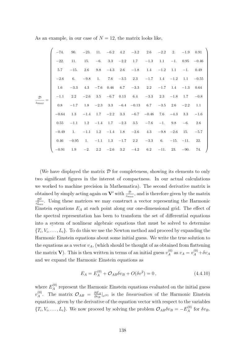
As an example, in our case of N = 12, the matrix looks like,

Dzmax

=

−74. 90. −23. 11. −6.2 4.2 −3.2 2.6 −2.2 2. −1.9 0.91

−22. 11. 15. −6. 3.3 −2.2 1.7 −1.3 1.1 −1. 0.95 −0.46

5.7 −15. 2.6 9.8 −4.3 2.6 −1.8 1.4 −1.2 1.1 −1. 0.49

−2.6 6. −9.8 1. 7.6 −3.5 2.3 −1.7 1.4 −1.2 1.1 −0.55

1.6 −3.3 4.3 −7.6 0.46 6.7 −3.3 2.2 −1.7 1.4 −1.3 0.64

−1.1 2.2 −2.6 3.5 −6.7 0.13 6.4 −3.3 2.3 −1.8 1.7 −0.8

0.8 −1.7 1.8 −2.3 3.3 −6.4 −0.13 6.7 −3.5 2.6 −2.2 1.1

−0.64 1.3 −1.4 1.7 −2.2 3.3 −6.7 −0.46 7.6 −4.3 3.3 −1.6

0.55 −1.1 1.2 −1.4 1.7 −2.3 3.5 −7.6 −1. 9.8 −6. 2.6

−0.49 1. −1.1 1.2 −1.4 1.8 −2.6 4.3 −9.8 −2.6 15. −5.7

0.46 −0.95 1. −1.1 1.3 −1.7 2.2 −3.3 6. −15. −11. 22.

−0.91 1.9 −2. 2.2 −2.6 3.2 −4.2 6.2 −11. 23. −90. 74.

(We have displayed the matrix D for completeness, showing its elements to only

two significant figures in the interest of compactness. In our actual calculations

we worked to machine precision in Mathematica). The second derivative matrix is

obtained by simply acting again onV′ with Dzmax

, and is therefore given by the matrixD2

z2max. Using these matrices we may construct a vector representing the Harmonic

Einstein equations EA at each point along our one-dimensional grid. The effect of

the spectral representation has been to transform the set of differential equations

into a system of nonlinear algebraic equations that must be solved to determine

Ti, Vi, . . . , Li. To do this we use the Newton method and proceed by expanding the

Harmonic Einstein equations about some initial guess. We write the true solution to

the equations as a vector vA, (which should be thought of as obtained from flattening

the matrix V). This is then written in terms of an initial guess v(0)A as vA = v

(0)A +δvA

and we expand the Harmonic Einstein equations as

EA = E(0)A +OABδvB +O(δv2) = 0 , (4.4.10)

where E(0)A represent the Harmonic Einstein equations evaluated on the initial guess

v(0)A . The matrix OAB = ∂EA

∂vB|v(0) is the linearisation of the Harmonic Einstein

equations, given by the derivative of the equation vector with respect to the variables

Ti, Vi, . . . , Li. We now proceed by solving the problem OABδvB = −E(0)A for δvB.

138

Using this solution one may then iteratively update the guess vector v(0)A , ultimately

obtaining a solution to the full nonlinear problem EA = 0. We must now turn to

a discussion of our choice for this initial guess and moreover how to implement the

boundary conditions for the original differential equation system in this discretised

framework.

We choose the background (reference) metric to be Schwarzchild with horizon at

z = 1

T (z) = 1− z ,

V (z) = 1 ,

A(z) = 0 ,

S(z) = 1 . (4.4.11)

Notice that the horizon of the reference metric is at z = 1 and this is ultimately the

reason we chose our grid to cover the interval [0, zmax]. (Although in this ingoing

formalism, the position of the reference metric horizon does not coincide with the

horizon of solutions, they should be close to one another and by choosing the refer-

ence horizon to be within our grid, we can hope that this will also be true for the

solutions we seek).

As an initial data, we take throughout the domain

T init(z) = T (z) ,

V init(z) = V (z) ,

Ainit(z) = A(z) ,

Sinit(z) = S(z) ,

P init(z) =−1 + (−1 + z)Qinit(z)2

2Qinit(z),

Qinit(z) = 1− 0.6z ,

Linit(z) = −0.8z , (4.4.12)

where in summary we have chosen the initial guess for the metric to equal the refer-

ence metric. For the aether we chose a guess consistent with it being asymptotically

coincident with the timelike Killing vector and smooth at the metric horizon. Hav-

ing chosen this behaviour for Qinit(z), the function P init(z) is then fixed by requiring

that the aether constraint (u2 + 1) = 0 is satisfied. The Lagrange multiplier is not

independent (see (1.4.69)) so in principle one can calculate a suitable initial guess

(as well as its asymptotic behaviour) from what we have already chosen. We simply

139

engineered that it vanish sufficiently quickly at infinity.

All that remains is to impose appropriate boundary data. We impose asymptotic

flatness at z = 0 as well as the requirement that the aether field coincide with the

static Killing vector asymptotically. Moreover, it is important to ensure the initial

guess satisfies the boundary conditions and hence the asymptotic behaviour of the

Lagrange multiplier is chosen also to match the above, so that we have

F0 = F init(z = 0) , (4.4.13)

where F init(z) = T init(z), V init(z), . . . Linit(z) and F0 is as defined below equation

(4.4.7). All these boundary variables are hence fixed to equal their initial values and

need not be updated in the Newton method iterations. (They should hence be left

out of the computation of the linearised Harmonic Einstein equations OAB).

As explained in the previous section where the ingoing methods were introduced,

we will also need to impose a single additional boundary condition at the innermost

point of the domain. This fixes the single modulus of these spherically symmetric

solutions, namely the mass. We choose

TN−1 = T init(z = zmax) , (4.4.14)

and hence TN−1 should also not be updated during the iterations. (Note that if

one does not impose this extra condition to fix the mass modulus, what one finds is

that the linearised operator in the Newton method OAB has zero modes indicating

that not enough data has been fixed. This can be seen even at the level of using

the ingoing methods to setup the problem of finding the Schwarzchild solution in

pure general relativity). We have now specified the problem completely and can

proceed to solve the equation system (4.4.10) iteratively using Mathematica. We

found that if one attempts to immediately solve the full problem as specified above,

the iterative procedure generically fails to converge to a solution. It turns out to be

extremely useful to first relax the aether field on a fixed gravitational background.

That is to say, it is useful to first solve the problem

Eaeα = 0 , (4.4.15)

where Eaeα schematically represents the aether and constraint equations on a fixed

gravitational background. (We use the index α rather than A to stress the fact

that this index is not running over all the variables but only the aether and con-

straint variables). This ‘preparatory’ problem is then solved as before using the

140

Newton method (updating the aether guess on the fixed gravitational background

corresponding to the initial guess (4.4.12)). Having done this, we may then use the

solution to this relaxation as initial data for the full problem which then quickly

converges to a solution.

Numerical Results

We now turn to a discussion of the results of our calculations. We solved equation

(4.4.10) iteratively by the Newton method, relaxing the aether first according to

(4.4.15) and then proceeding with the full problem. From the resulting vector that

solves the system, one can compute interpolating polynomials that approximate the

functions T (z), V (z), . . . , L(z). These are displayed in Figure 4.1 and together

constitute the metric and aether functions of a numerical static, spherically sym-

metric black hole in Einstein-Aether theory. The solution displayed corresponds to

a black hole with c1 = 0.4 and has a mass that is implicitly determined by our choice

of boundary data at the innermost point TNN . That is to say, changing the data

there, will change the mass of the solution, thus moving along the one-parameter

family of solutions.

The mass MT of this black hole solution can be computed by the usual ADM

prescription by examining the coefficient of the O(z) term in the gνν component of

the metric [228]. We then have that

2GMADM = −T ′(0) , (4.4.16)

where G is the gravitational constant that appears in the Einstein-Aether action.

For the solution of Figure 4.1, we may readily compute that 2GMADM = 1.03(3)

and the metric horizon is at zh = 0.997(4), (defined by T (zh) = 0).

To highlight some of the qualitative differences between black holes in Einstein-

Aether and general relativity, it is instructive to consider a plot of the function√

S(z)(T (z) − 1)/2. We display this in Figure 4.3 for the static aether black hole

of Figure 4.1. For Schwarzchild solutions in pure general relativity, this quantity

is a constant that is proportional to the mass of the black hole. In contrast, in

Einstein-Aether theory we see that it varies as a function of z (and moreover one

can show the deviation from general relativity is dependent on c1). We also plot

φ = ξµξµ for our static aether black hole in Figure 4.2 to verify that it vanishes on

our solutions and hence that we have a true (as opposed to solitonic) solution.

We may now repeat the procedure outlined above, changing c1 to investigate

the structure of black holes in Einstein-Aether theory for different values of this

141

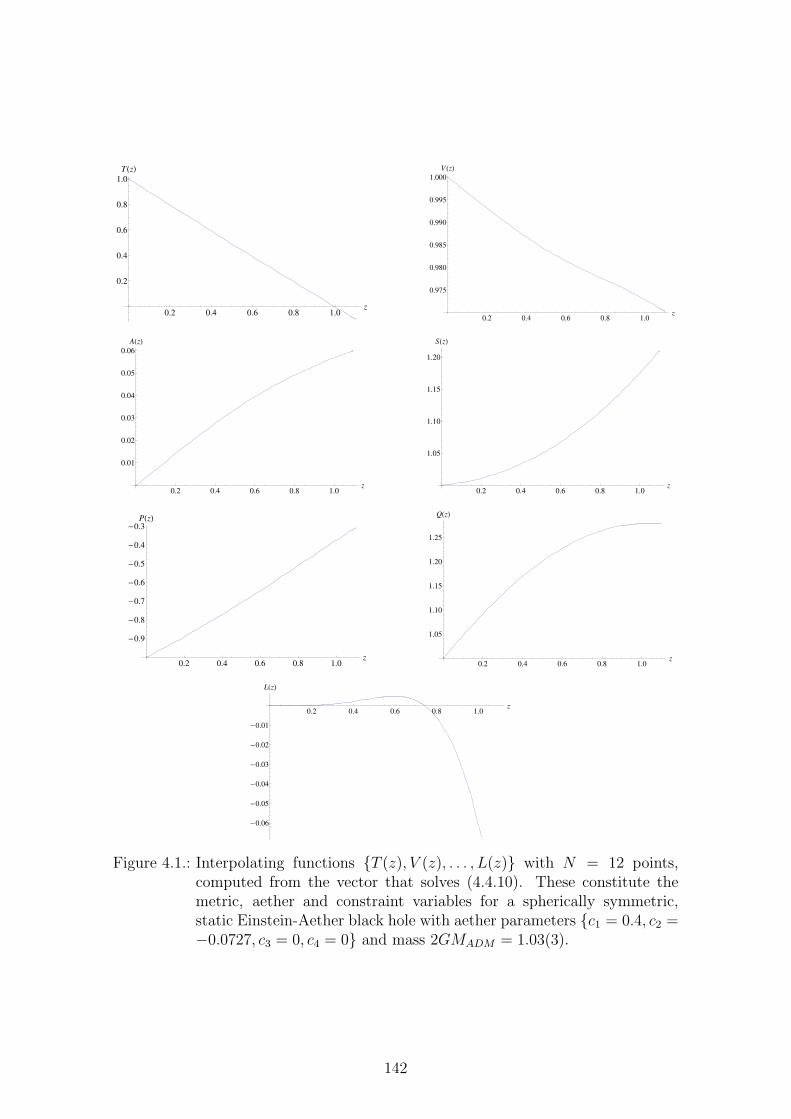
0.2 0.4 0.6 0.8 1.0z

0.2

0.4

0.6

0.8

1.0

THzL

0.2 0.4 0.6 0.8 1.0z

0.975

0.980

0.985

0.990

0.995

1.000

V HzL

0.2 0.4 0.6 0.8 1.0z

0.01

0.02

0.03

0.04

0.05

0.06

AHzL

0.2 0.4 0.6 0.8 1.0z

1.05

1.10

1.15

1.20

SHzL

0.2 0.4 0.6 0.8 1.0z

-0.9

-0.8

-0.7

-0.6

-0.5

-0.4

-0.3PHzL

0.2 0.4 0.6 0.8 1.0z

1.05

1.10

1.15

1.20

1.25

QHzL

0.2 0.4 0.6 0.8 1.0z

-0.06

-0.05

-0.04

-0.03

-0.02

-0.01

LHzL

Figure 4.1.: Interpolating functions T (z), V (z), . . . , L(z) with N = 12 points,computed from the vector that solves (4.4.10). These constitute themetric, aether and constraint variables for a spherically symmetric,static Einstein-Aether black hole with aether parameters c1 = 0.4, c2 =−0.0727, c3 = 0, c4 = 0 and mass 2GMADM = 1.03(3).

142

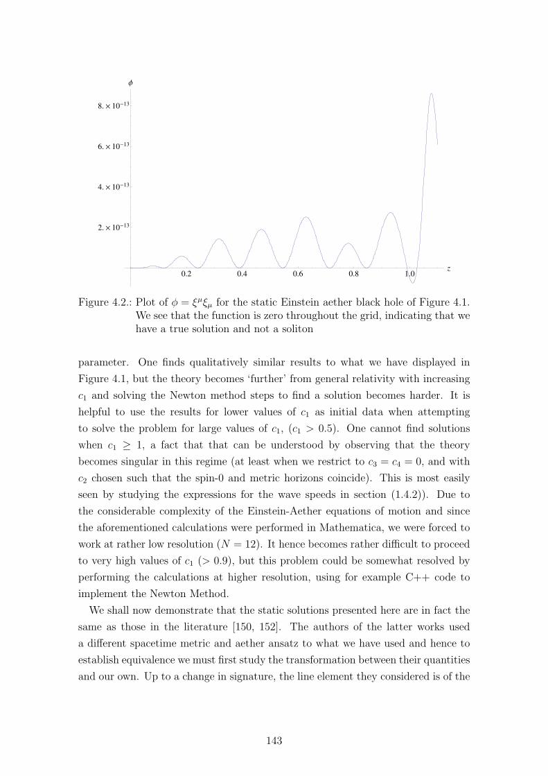
0.2 0.4 0.6 0.8 1.0z

2.´ 10-13

4.´ 10-13

6.´ 10-13

8.´ 10-13

Φ

Figure 4.2.: Plot of φ = ξµξµ for the static Einstein aether black hole of Figure 4.1.We see that the function is zero throughout the grid, indicating that wehave a true solution and not a soliton

parameter. One finds qualitatively similar results to what we have displayed in

Figure 4.1, but the theory becomes ‘further’ from general relativity with increasing

c1 and solving the Newton method steps to find a solution becomes harder. It is

helpful to use the results for lower values of c1 as initial data when attempting

to solve the problem for large values of c1, (c1 > 0.5). One cannot find solutions

when c1 ≥ 1, a fact that that can be understood by observing that the theory

becomes singular in this regime (at least when we restrict to c3 = c4 = 0, and with

c2 chosen such that the spin-0 and metric horizons coincide). This is most easily

seen by studying the expressions for the wave speeds in section (1.4.2)). Due to

the considerable complexity of the Einstein-Aether equations of motion and since

the aforementioned calculations were performed in Mathematica, we were forced to

work at rather low resolution (N = 12). It hence becomes rather difficult to proceed

to very high values of c1 (> 0.9), but this problem could be somewhat resolved by

performing the calculations at higher resolution, using for example C++ code to

implement the Newton Method.

We shall now demonstrate that the static solutions presented here are in fact the

same as those in the literature [150, 152]. The authors of the latter works used

a different spacetime metric and aether ansatz to what we have used and hence to

establish equivalence we must first study the transformation between their quantities

and our own. Up to a change in signature, the line element they considered is of the

143

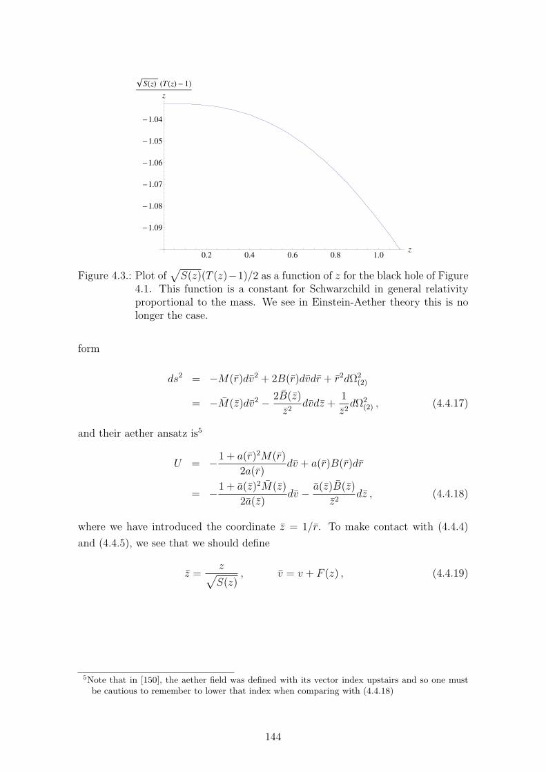
0.2 0.4 0.6 0.8 1.0z

-1.09

-1.08

-1.07

-1.06

-1.05

-1.04

SHzL HTHzL- 1Lz

Figure 4.3.: Plot of√

S(z)(T (z)−1)/2 as a function of z for the black hole of Figure4.1. This function is a constant for Schwarzchild in general relativityproportional to the mass. We see in Einstein-Aether theory this is nolonger the case.

form

ds2 = −M(r)dv2 + 2B(r)dvdr + r2dΩ2(2)

= −M(z)dv2 − 2B(z)

z2dvdz +

1

z2dΩ2

(2) , (4.4.17)

and their aether ansatz is5

U = −1 + a(r)2M(r)

2a(r)dv + a(r)B(r)dr

= −1 + a(z)2M(z)

2a(z)dv − a(z)B(z)

z2dz , (4.4.18)

where we have introduced the coordinate z = 1/r. To make contact with (4.4.4)

and (4.4.5), we see that we should define

z =z

√

S(z), v = v + F (z) , (4.4.19)

5Note that in [150], the aether field was defined with its vector index upstairs and so one mustbe cautious to remember to lower that index when comparing with (4.4.18)

144

for some function F (z), and equality of the two forms then requires that

T (z) = M

(

z√

S(z)

)

, (4.4.20)

V (z) = M

(

z√

S(z)

)

F′(z)z2 + B

(

z√

S(z)

)

√

S(z)

(

1− zS′(z)

2S(z)

)

, (4.4.21)

A(z) = z2F

′(z)

(

−M

(

z√

S(z)

)

F′(z)z2 − 2B

(

z√

S(z)

)

√

S(z)

×(

1− zS′(z)

2S(z)

))

, (4.4.22)

P (z) = − 1

2a

(

z√S(z)

)2

1 + a

(

z√

S(z)

)2

M

(

z√

S(z)

)

, (4.4.23)

Q(z) =1

2a

(

z√S(z)

)2

1 + a

(

z√

S(z)

)2

M

(

z√

S(z)

)

F′(z)z2

+ a

(

z√

S(z)

)

B

(

z√

S(z)

)

√

S(z)

(

1− zS′(z)

2S(z)

)

. (4.4.24)

Having established these transformations, we repeated the shooting calculations of

[150], to obtain their static aether black holes6. In detail, for the aether parameters

c1 = 0.4, c2 = −0.0727, c3 = c4 = 0, we integrated inwards from z = 1/100 to

z = 1000 to obtain a solution. (Note once again that the metric horizon has been

chosen to coincide with the spin-0 horizon). The asymptotic expansions of the field

equations contain two pieces of data

M(z) = 1 +M1 z +c1M

31

48z3 + . . . ,

B(z) = 1 +c1M

21

16z2 − c1M

31

12z3 + . . . ,

a(z) = 1− M1

2z + a2 z

2 − M1 (96 a2 + (−6 + c1)M21 )

96z3 + . . . , (4.4.25)

namely M1 and a2. We fixed M1 = −1.00327(0)7, and tuned a2 so as to achieve

regularity at the spin-0 horizon. In more detail, regularity at the spin-zero horizon

is implemented by observing that B(z) satisfies B′(z) = b0M(z)

+ . . . and thus at the

horizon, where M(z) → 0, we require as a ‘regularity condition’ that the function

b0 = 0 [150]. (The ellipses denote terms that are finite in this limit). Given M1,

6There is a slight subtlety here, namely that unlike in the shooting of [150], we did not scale ourr coordinate such that the horizon lies precisely at r = 1. One needs to make this additionaltransformation if a comparison of observables (such as with Table I of [150]) is desired.

7We used our spectral solutions to read off M1 to high precision. This was then held fixed at thisvalue, with the remaining piece of data a2 being used as our shooting parameter.

145

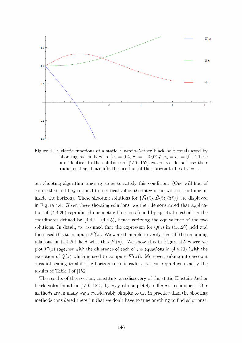
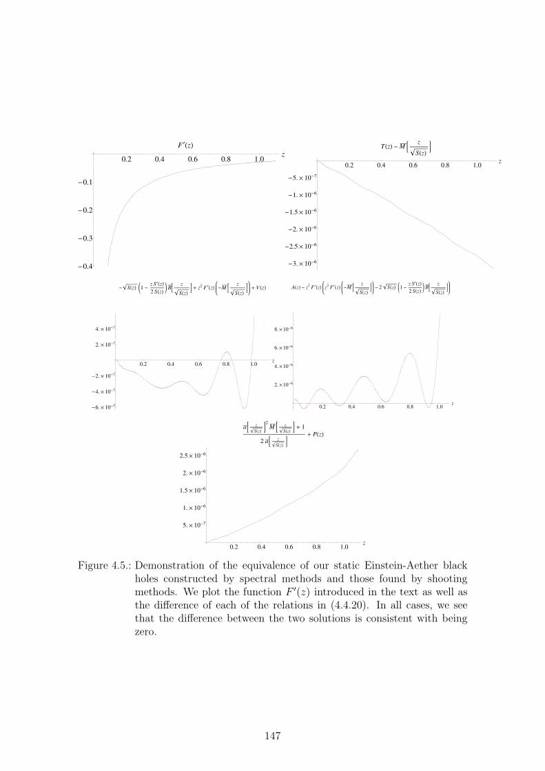
0.2 0.4 0.6 0.8 1.0z

-0.4

-0.3

-0.2

-0.1

F¢HzL0.2 0.4 0.6 0.8 1.0

z

-3.´ 10-6

-2.5´ 10-6

-2.´ 10-6

-1.5´ 10-6

-1.´ 10-6

-5.´ 10-7

THzL -M B z

SHzL F

0.2 0.4 0.6 0.8 1.0z

-6.´ 10-7

-4.´ 10-7

-2.´ 10-7

2.´ 10-7

4.´ 10-7

- SHzL K1 - z S¢HzL2 SHzL O BB z

SHzL F + z2 F¢HzL -M B z

SHzL F + V HzL

0.2 0.4 0.6 0.8 1.0z

2.´10-6

4.´10-6

6.´10-6

8.´10-6

AHzL- z2 F¢HzL z2 F¢HzL -M B z

SHzL F - 2 SHzL K1- z S¢HzL2 SHzL O BB z

SHzL F

0.2 0.4 0.6 0.8 1.0z

5.´ 10-7

1.´ 10-6

1.5´ 10-6

2.´ 10-6

2.5´ 10-6

aB z

SHzL F2

M B z

SHzL F + 1

2 aB z

SHzL F+ PHzL

Figure 4.5.: Demonstration of the equivalence of our static Einstein-Aether blackholes constructed by spectral methods and those found by shootingmethods. We plot the function F ′(z) introduced in the text as well asthe difference of each of the relations in (4.4.20). In all cases, we seethat the difference between the two solutions is consistent with beingzero.

147

Moreover, regularity at the spin-zero horizon is encoded from the start in our ap-

proach by use of the ingoing techniques detailed in the previous section and we do

not need to impose this a-posteriori. The real power of these new techniques how-

ever is that they readily extend (with little more than technical differences) to the

stationary case.

4.5. Stationary Black Hole Solutions

We may now proceed to apply the techniques of the previous section to the more

complex problem of constructing stationary, rotating black holes in Einstein-Aether

theory. We begin with the metric

ds2 = −T (z, θ) dv2 − 2W (z, θ) sin2 θ dvdφ− 2V (z, θ)

z2dvdz

+2U(z, θ) sin θ

zdvdθ +

S(z, θ) sin2 θ

z2dφ2 +

2P (z, θ) sin2 θ

z2dφdz

+2Q(z, θ) sin θ

z2dφdθ +

A(z, θ)

z4dz2 +

B(z, θ)

z2dθ2

+2F (z, θ) sin θ

z2dzdθ , (4.5.26)

together with the aether ansatz,

U = H(z, θ)dv + J(z, θ) sin2 θdφ− X(z, θ)

z2dz +

Y (z, θ) sin θ

zdθ , (4.5.27)

where once again, v is an ingoing time coordinate and z is an inverse radial coordi-

nate. By the assumption of stationarity, ∂∂v

and ∂∂φ

are Killing vectors and hence the

functions that appear in both (4.5.26) and (4.5.27) depend non-trivially on only the

(z, θ) coordinates. We still however have the full number of ten metric components

and four aether components to determine together with the Lagrange multiplier

constraint λ(z, θ) = z3L(z, θ). The equations of motion that follow from this ansatz

constitute a complicated PDE problem in two variables and the shooting techniques

that have been used thus far in the literature to construct static solutions are not

applicable outside the case of ODEs. Fortunately, the numerical methods discussed

in the previous section naturally extend to multivariate problems.

To proceed, we begin as before, this time discretising both the z and θ directions

to form a tensor product grid structure with Nz×Nθ points [227]. We shall describe

two distinct discretisation procedures and present the results that follow from each

in turn. As usual, with our ingoing methods, it is important to choose coordinates

such that the radial patch extends into the interior of the metric horizon. We

148

shall consider the radial range 0 ≤ z ≤ zmax = 0.6, with z = 0 corresponding

to infinity (and by a suitable choice of background metric, we can ensure that the

aforementioned constraint is satisfied and the metric horizon lies inside our grid).

By symmetry, we can without loss of generality consider the polar angle in the range

0 ≤ θ ≤ θmax = π/2. The first discretisation scheme we consider is analogous to

that used in the static case and uses Chebyshev grids independently in both the z

and θ directions and spectral representations of derivative operators. In detail we

consider a 2D tensor product grid with Nz = Nθ = 20

zi =

zmax

2

(

1 + cos

(

iπ

Nz − 1

))

for i = 0, . . . , (Nz − 1) ,

θj =

θmax

2

(

1 + cos

(

jπ

Nθ − 1

))

for j = 0, . . . , (Nθ − 1) , (4.5.28)

in terms of which the metric, aether and constraint functions are discretised as

Fij = F(z(Nz−1)−i, θ(Nθ−1)−j), with F(zi, θj) = T (zi, θj),W (zi, θj), . . . , L(zi, θj).One may then construct the 1D Chebyshev differentiation matrices Dz and Dθ (of

sizes Nz × Nz and Nθ × Nθ respectively), as before using the definition (4.4.9).

The full 2D derivative matrices may then be computed from these matrices as ten-

sor products. That is to say, if we represent our functions across the grid as an

array of the form F cij, (where the new index c = 0, . . . , 14 labels which met-

ric/aether/constraint component we are considering), then we have that

∂

∂zF c

I = (⊗Dz)IJF cJ ,

∂

∂θF c

I = (Dθ ⊗ )IJF cJ ,

∂2

∂z2F c

I = (⊗D2z)IJF c

J ,

∂2

∂θ2F c

I = (D2θ ⊗ )IJF c

J ,

∂2

∂z∂θF c

I = (Dz ⊗Dθ)IJF cJ . (4.5.29)

The F cI are the components of the vector that are obtained from flattening the matrix

F cij8. From (4.5.29), one may then assemble the equations of motion across the 2D

grid, which are then turned into a vector which we write schematically as EA. We

may then proceed to solve the system by the Newton method, exactly as before in the

8The ordering of the tensor products in (4.5.29) depends on the ordering of the flattening oper-ation, that is to say the ordering of the multiplication in the tensor product may be reversedfrom what is written here depending on whether flattening is done row by row or column bycolumn.

149

static case: One begins by expanding the equations as EA = E(0)A +OABδvB+O(v2),

(where in analogy with the static case, vA is the flattened vector constructed from

F cJ viewed as an array in (c, J) and using the same notation as we used there, v

(0)A

is some initial guess and E(0)A the equations evaluated on this initial guess). We

then solve OABδvB = −E(0)A

9 iteratively updating vA, eventually converging to a

solution of the full non-linear problem EA = 0. As before in the static case, in our

experience it is essential to first relax the aether field and constraint equations on a

fixed gravitational background before tackling the full problem.

The second discretisation scheme we consider is finite differencing (6th order).

The only difference compared with the spectral methods outlined above is in the

splitting of the (z, θ) intervals and the construction of the derivative matrices Dz

and Dθ. Instead of (4.5.28), we use a tensor product grid defined by

Zi = zmin + i

(zmax − zmin

Nz − 1

)

,

Θi = θmin + i

(θmax − θmin

Nz − 1

)

for i = 0, . . . , Nz − 1 , (4.5.30)

(where we recall that in our case, zmin = θmin = 0, zmax = 0.6, and θmax = π/2).

Notice that unlike the Chebyshev grids where points cluster at the end points of

the intervals, finite difference grids consist of evenly spaced points. The derivative

matrices Dz,Dθ are then constructed by way of a polynomial interpolation of order

m (m = 6 for 6th order differencing). (Note that the precise details of the stencils we

use are described in [229] and in the Mathematica tutorial ”Numerical Solution to

Partial Differential Equations”. Schematically, these methods work by constructing

a stencil with general coefficients and using Pade approximations to compute these

coefficients so as to make the stencil accurate for as high degree polynomials as

possible. Moreover these methods automatically minimise errors at any boundaries

in the problem).

The mechanics of solving the system then proceeds exactly as in the spectral

case, constructing the 2D derivative matrices as tensor products, assembling the

equations of motion from these and solving the system by the Newton method.

Whilst spectral methods have the advantage of being able to achieve high accuracy

even at relatively low resolution (any loss of accuracy that can arise there due to the

Runge phenomena can in practice be minimised by using a Cheyshev as opposed

to an even grid), the difficulty with them is that they only work well when the

9Instead of symbolically differentiating the equations with respect to the discretised variables asin the static case to calculate OAB , we found it much more efficient here to compute it as a

central difference OAB = EA(v+δv)−EA(v+δv)2∆ where the vector δvA = ∆δAB .

150

functions to be solved for are very smooth (formally ∞). In the case of black holes

in Einstein-Aether theory, one can show that the metric functions are not ∞ at

z = 0 due to log terms in the expansion (specifically terms of the form z2 log z and

higher order contributions). Indeed we find as a consequence of this that for large

deviations from general relativity c1 > 0.6, spectral methods seem to struggle to

converge to solutions. It therefore appears that finite difference techniques are more

robust for our purposes.

Having specified our discretisation schemes, all that remains to be done to solve

the system is to choose a suitable background metric and initial guess together with

appropriate boundary conditions for the PDE problem in question. We must also

fix two pieces of boundary data at z = zmax to fix the angular velocity and mass

moduli associated to stationary solutions.

In the regime where c1 is small, the theory is parametrically close to general

relativity and thus any stationary black holes should resemble the Kerr solution. We

therefore choose Kerr for the reference metric, that is to say, we choose a reference

line element of the form (4.5.26) with

T (z, θ) = 1− 2M2z

Σ(z, θ),

V (z, θ) = M ,

W (z, θ) =2aM2z

Σ(z, θ),

S(z, θ) =1

Σ(z, θ)

((M2 + a2z2)2 − z2∆(z)a2 sin2 θ

),

P (z, θ) = Ma ,

B(z, θ) = Σ(z, θ) ,

U(z, θ) = 0 ,

Q(z, θ) = 0 ,

A(z, θ) = 0 ,

F (z, θ) = 0 , (4.5.31)

where Σ(z, θ) = M2 + a2z2 cos2 θ and ∆(z) = M2 − 2M2z + a2z2. Moreover

as an initial guess, we begin with metric functions equal to those of the Kerr

metric T init(z, θ) = T (z, θ), . . . , F init(z, θ) = F (z, θ). For the aether functions

151

X init(z, θ), Y init(z, θ) and constraint Linit(z, θ) we choose

X init(z, θ) = M(1 + 0.4z) ,

Y init(z, θ) = 0 ,

Linit(z, θ) = −0.01z2 , (4.5.32)

whilst for the remaining aether components, we take J init(z, θ) = −aH init(z, θ), and

solve for H init(z, θ) by demanding that the aether constraint u2 + 1 = 0 is satisfied

by the initial guess. (The precise form of the function H init(z, θ) is rather unsightly

and hence we do not include it here).

As with the static case, we impose Dirichlet boundary conditions at z = 0 (infin-

ity), and demand that all functions equal their initial values there

F0j = F init(z = 0, θ = θ(Nθ−1)−j) ∀j , (4.5.33)

(where Fij is as defined below equation (4.5.29)). This condition is of course equiva-

lent to imposing asymptotic flatness for the metric components. These components

should not be updated during the Newton method iterations. The new feature in

the stationary case is that we must also impose appropriate boundary conditions at

the axis of rotational symmetry. By the regularity analysis of section 3.4.3, we know

that all functions in the problem should have expansions with no terms linear in θ

at this axis, and thus we impose Neumann boundary data for all the metric, aether

and constraint components at θ = 0

∂

∂θFi0 = 0 ∀i . (4.5.34)

On the other hand, we must ensure that all functions are even about the ‘mirror

plane’ corresponding to the θ = π/2 boundary (which is of course an artificial con-

struction that we introduced as the region π/2 < θ ≤ π carries no new information).

This is achieved by imposing Dirichlet conditions for all functions that appear in

the metric/aether ansatze as odd in dθ

Gi (Nc−1) = Ginit(z = z(Nz−1)−i, θ = π/2) = 0 ∀i , (4.5.35)

where Gij = Fij, Uij, Qij, Yij, and imposing Neumann conditions for the remaining

variables

∂

∂θHi (Nc−1) = 0 ∀i , (4.5.36)

152

where Hij = Tij, Vij,Wij, Sij, Pij, Bij, Aij, Xij, Lij, Jij, Hij.There is an additional subtlety at the axis in these ingoing methods. Whilst

regularity at the horizon is automatic in our chart, at the axis we would expect

to have to impose the additional regularity condition of section 3.4.3, namely that

B(z, θ = 0) = S(z, θ = 0). Recall though that this condition should be thought of

as a arising as a consequence of smoothness at the axis and since our initial guess for

the metric (Kerr) is smooth and the Newton method updates preserve smoothness

we expect that this condition is automatically satisfied and need not be imposed.

Indeed we will explicitly check that this is so and that it is satisfied for the numerical

solutions we find.

Finally, following the ingoing horizon prescription, we must fix the two moduli

associated to our solution by imposing two additional conditions at the innermost

points of our domain. We do this by imposing

T(Nz1)(Nc−1) = T init(z = zmax, θ = θmax) ,

W(Nz1)(Nc−1) = W init(z = zmax, θ = θmax) , (4.5.37)

which fixes the mass and angular momentum moduli of the system. Note that one

can in principle fix any two functions at zmax, θmax, but we choose T (z, θ), and

W (z, θ) as they work well. As with the static case, if one does not impose these con-

ditions to fix the moduli, the linearisation of the equations OAB has zero modes and

one will not find a solution. We may now turn to a discussion of the results we have

found on implementing the numerical setup described in this section. We performed

all calculations in C++, outputting data to Mathematica (and using this to display

our interpolations). The Einstein-Aether equations were built systematically in a

subroutine in C++ that calculates them at a given point in our domain. In detail

we broke these equations down into their constituent zero, one and two derivative

pieces involving the metric and aether. These pieces (schematically ∂g, ∂∂g, ∂u, ∂∂u

etc) were then computed symbolically in Mathematica on our ansatz and then out-

putted to C++ as arrays that the subroutine assembles into the full equations. By

calling this subroutine throughout the grid (given initial data) one can then cal-

culate the Einstein-Aether equations throughout the domain. (Note that in places

where Dirichlet boundary conditions are imposed, such as at z = 0, the routine

does not need to be called as those points are not updated in the Newton method

iterations. Moreover, on boundaries which have Neumann conditions, instead of

calling the Einstein-Aether equations we impose the Neumann boundary condition

explicitly as an equation in the equation-vector EA). Our code uses this routine to

153

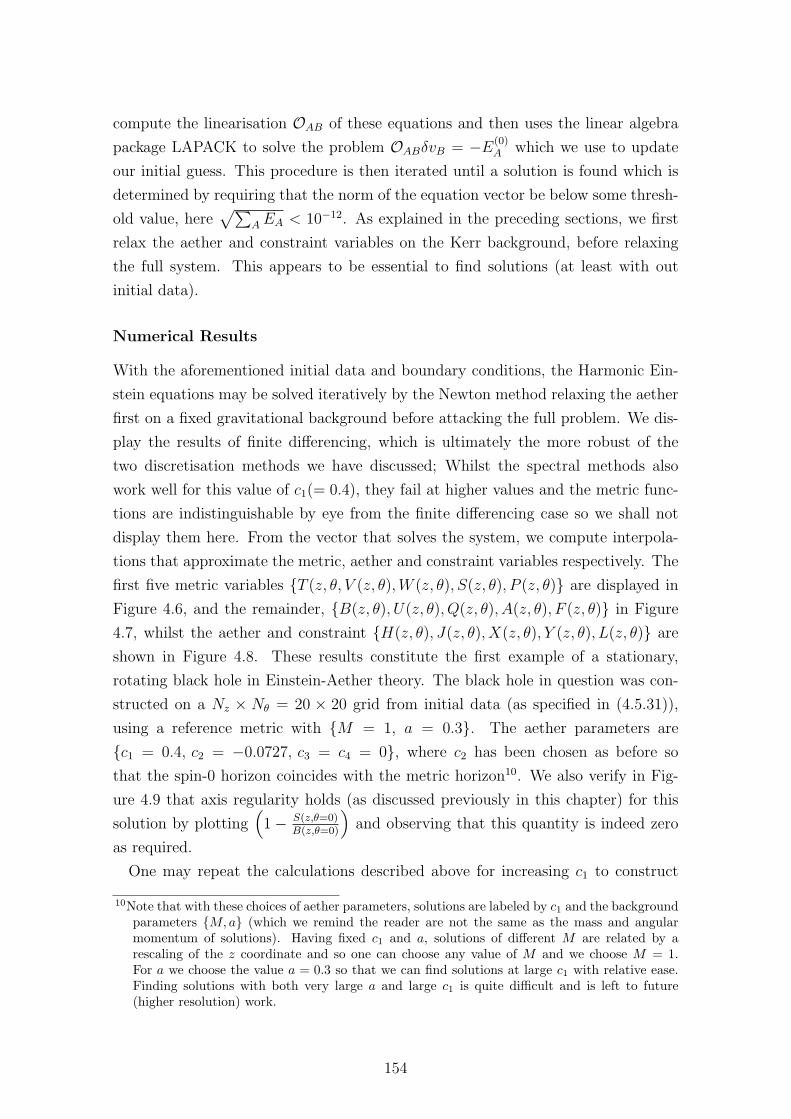
compute the linearisation OAB of these equations and then uses the linear algebra

package LAPACK to solve the problem OABδvB = −E(0)A which we use to update

our initial guess. This procedure is then iterated until a solution is found which is

determined by requiring that the norm of the equation vector be below some thresh-

old value, here√∑

AEA < 10−12. As explained in the preceding sections, we first

relax the aether and constraint variables on the Kerr background, before relaxing

the full system. This appears to be essential to find solutions (at least with out

initial data).

Numerical Results

With the aforementioned initial data and boundary conditions, the Harmonic Ein-

stein equations may be solved iteratively by the Newton method relaxing the aether

first on a fixed gravitational background before attacking the full problem. We dis-

play the results of finite differencing, which is ultimately the more robust of the

two discretisation methods we have discussed; Whilst the spectral methods also

work well for this value of c1(= 0.4), they fail at higher values and the metric func-

tions are indistinguishable by eye from the finite differencing case so we shall not

display them here. From the vector that solves the system, we compute interpola-

tions that approximate the metric, aether and constraint variables respectively. The

first five metric variables T (z, θ, V (z, θ),W (z, θ), S(z, θ), P (z, θ) are displayed in

Figure 4.6, and the remainder, B(z, θ), U(z, θ), Q(z, θ), A(z, θ), F (z, θ) in Figure

4.7, whilst the aether and constraint H(z, θ), J(z, θ), X(z, θ), Y (z, θ), L(z, θ) are

shown in Figure 4.8. These results constitute the first example of a stationary,

rotating black hole in Einstein-Aether theory. The black hole in question was con-

structed on a Nz × Nθ = 20 × 20 grid from initial data (as specified in (4.5.31)),

using a reference metric with M = 1, a = 0.3. The aether parameters are

c1 = 0.4, c2 = −0.0727, c3 = c4 = 0, where c2 has been chosen as before so

that the spin-0 horizon coincides with the metric horizon10. We also verify in Fig-

ure 4.9 that axis regularity holds (as discussed previously in this chapter) for this

solution by plotting(

1− S(z,θ=0)B(z,θ=0)

)

and observing that this quantity is indeed zero

as required.

One may repeat the calculations described above for increasing c1 to construct

10Note that with these choices of aether parameters, solutions are labeled by c1 and the backgroundparameters M,a (which we remind the reader are not the same as the mass and angularmomentum of solutions). Having fixed c1 and a, solutions of different M are related by arescaling of the z coordinate and so one can choose any value of M and we choose M = 1.For a we choose the value a = 0.3 so that we can find solutions at large c1 with relative ease.Finding solutions with both very large a and large c1 is quite difficult and is left to future(higher resolution) work.

154

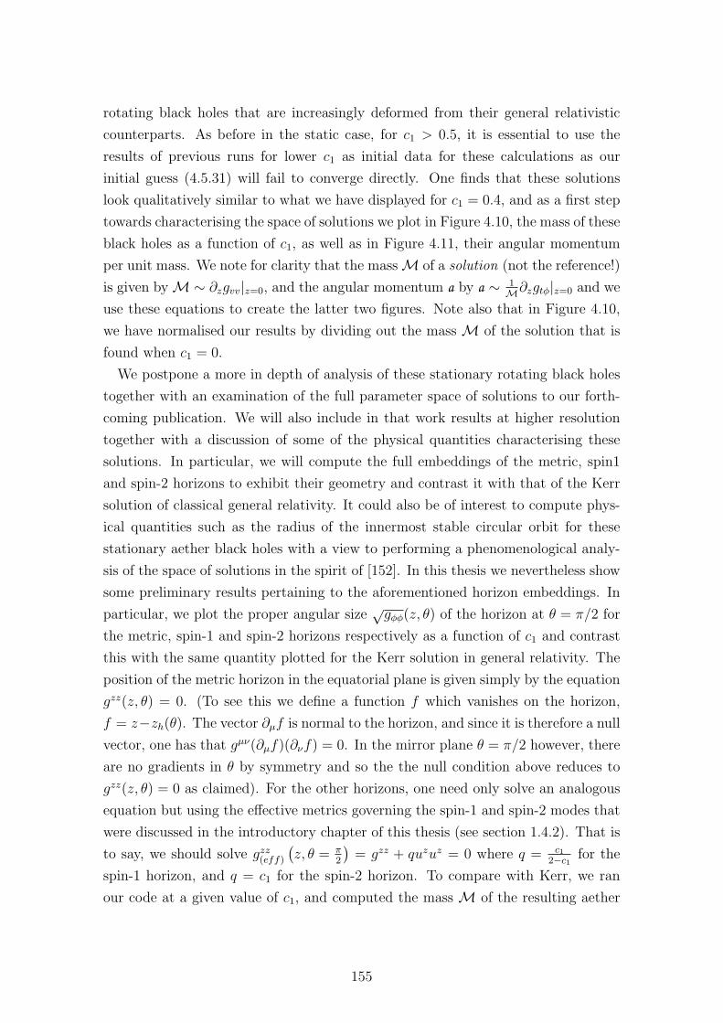
rotating black holes that are increasingly deformed from their general relativistic

counterparts. As before in the static case, for c1 > 0.5, it is essential to use the

results of previous runs for lower c1 as initial data for these calculations as our

initial guess (4.5.31) will fail to converge directly. One finds that these solutions

look qualitatively similar to what we have displayed for c1 = 0.4, and as a first step

towards characterising the space of solutions we plot in Figure 4.10, the mass of these

black holes as a function of c1, as well as in Figure 4.11, their angular momentum

per unit mass. We note for clarity that the mass M of a solution (not the reference!)

is given by M ∼ ∂zgvv|z=0, and the angular momentum a by a ∼ 1M∂zgtφ|z=0 and we

use these equations to create the latter two figures. Note also that in Figure 4.10,

we have normalised our results by dividing out the mass M of the solution that is

found when c1 = 0.

We postpone a more in depth of analysis of these stationary rotating black holes

together with an examination of the full parameter space of solutions to our forth-

coming publication. We will also include in that work results at higher resolution

together with a discussion of some of the physical quantities characterising these

solutions. In particular, we will compute the full embeddings of the metric, spin1

and spin-2 horizons to exhibit their geometry and contrast it with that of the Kerr

solution of classical general relativity. It could also be of interest to compute phys-

ical quantities such as the radius of the innermost stable circular orbit for these

stationary aether black holes with a view to performing a phenomenological analy-

sis of the space of solutions in the spirit of [152]. In this thesis we nevertheless show

some preliminary results pertaining to the aforementioned horizon embeddings. In

particular, we plot the proper angular size√gφφ(z, θ) of the horizon at θ = π/2 for

the metric, spin-1 and spin-2 horizons respectively as a function of c1 and contrast

this with the same quantity plotted for the Kerr solution in general relativity. The

position of the metric horizon in the equatorial plane is given simply by the equation

gzz(z, θ) = 0. (To see this we define a function f which vanishes on the horizon,

f = z−zh(θ). The vector ∂µf is normal to the horizon, and since it is therefore a null

vector, one has that gµν(∂µf)(∂νf) = 0. In the mirror plane θ = π/2 however, there

are no gradients in θ by symmetry and so the the null condition above reduces to

gzz(z, θ) = 0 as claimed). For the other horizons, one need only solve an analogous

equation but using the effective metrics governing the spin-1 and spin-2 modes that

were discussed in the introductory chapter of this thesis (see section 1.4.2). That is

to say, we should solve gzz(eff)(z, θ = π

2

)= gzz + quzuz = 0 where q = c1

2−c1for the

spin-1 horizon, and q = c1 for the spin-2 horizon. To compare with Kerr, we ran

our code at a given value of c1, and computed the mass M of the resulting aether

155

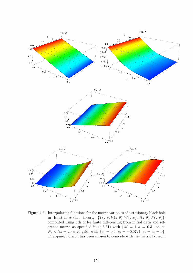
Figure 4.6.: Interpolating functions for the metric variables of a stationary black holein Einstein-Aether theory, T (z, θ, V (z, θ),W (z, θ), S(z, θ), P (z, θ),computed using 6th order finite differencing from initial data and ref-erence metric as specified in (4.5.31) with M = 1, a = 0.3 on anNz × Nθ = 20 × 20 grid, with c1 = 0.4, c2 = −0.0727, c3 = c4 = 0.The spin-0 horizon has been chosen to coincide with the metric horizon.

156

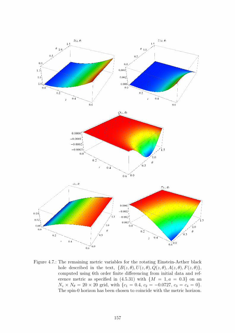
Figure 4.7.: The remaining metric variables for the rotating Einstein-Aether blackhole described in the text, B(z, θ), U(z, θ), Q(z, θ), A(z, θ), F (z, θ),computed using 6th order finite differencing from initial data and ref-erence metric as specified in (4.5.31) with M = 1, a = 0.3 on anNz × Nθ = 20 × 20 grid, with c1 = 0.4, c2 = −0.0727, c3 = c4 = 0.The spin-0 horizon has been chosen to coincide with the metric horizon.

157

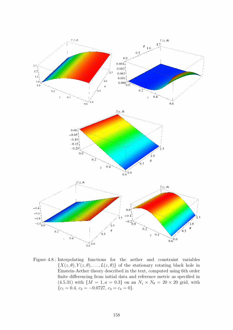
Figure 4.8.: Interpolating functions for the aether and constraint variablesX(z, θ), Y (z, θ), . . . , L(z, θ) of the stationary rotating black hole inEinstein-Aether theory described in the text, computed using 6th orderfinite differencing from initial data and reference metric as specified in(4.5.31) with M = 1, a = 0.3 on an Nz × Nθ = 20 × 20 grid, withc1 = 0.4, c2 = −0.0727, c3 = c4 = 0.

158

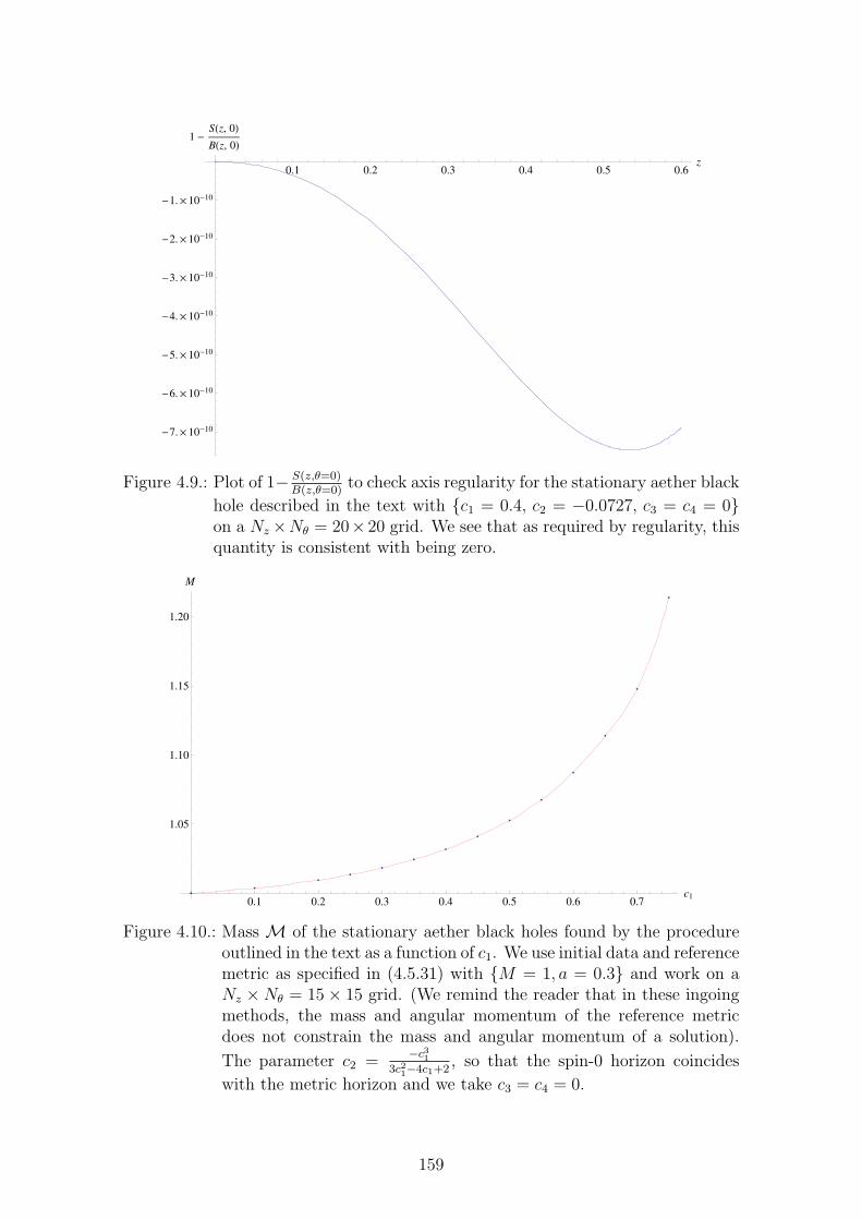
0.1 0.2 0.3 0.4 0.5 0.6z

-7.´10-10

-6.´10-10

-5.´10-10

-4.´10-10

-3.´10-10

-2.´10-10

-1.´10-10

1 -SHz, 0LBHz, 0L

Figure 4.9.: Plot of 1− S(z,θ=0)B(z,θ=0)

to check axis regularity for the stationary aether black

hole described in the text with c1 = 0.4, c2 = −0.0727, c3 = c4 = 0on a Nz ×Nθ = 20× 20 grid. We see that as required by regularity, thisquantity is consistent with being zero.

0.1 0.2 0.3 0.4 0.5 0.6 0.7c1

1.05

1.10

1.15

1.20

M

Figure 4.10.: Mass M of the stationary aether black holes found by the procedureoutlined in the text as a function of c1. We use initial data and referencemetric as specified in (4.5.31) with M = 1, a = 0.3 and work on aNz ×Nθ = 15× 15 grid. (We remind the reader that in these ingoingmethods, the mass and angular momentum of the reference metricdoes not constrain the mass and angular momentum of a solution).

The parameter c2 =−c31

3c21−4c1+2, so that the spin-0 horizon coincides

with the metric horizon and we take c3 = c4 = 0.

159

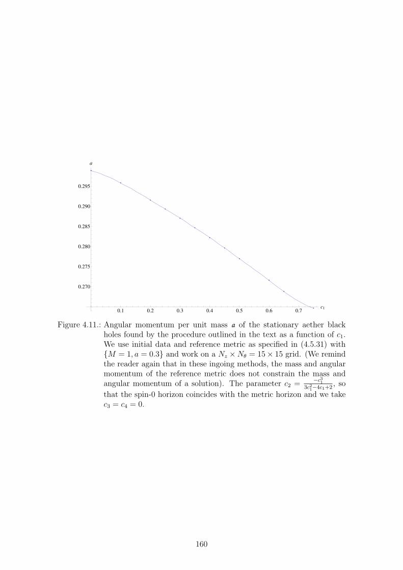
0.1 0.2 0.3 0.4 0.5 0.6 0.7c1

0.270

0.275

0.280

0.285

0.290

0.295

a

Figure 4.11.: Angular momentum per unit mass a of the stationary aether blackholes found by the procedure outlined in the text as a function of c1.We use initial data and reference metric as specified in (4.5.31) withM = 1, a = 0.3 and work on a Nz ×Nθ = 15× 15 grid. (We remindthe reader again that in these ingoing methods, the mass and angularmomentum of the reference metric does not constrain the mass andangular momentum of a solution). The parameter c2 =

−c313c21−4c1+2

, so

that the spin-0 horizon coincides with the metric horizon and we takec3 = c4 = 0.

160

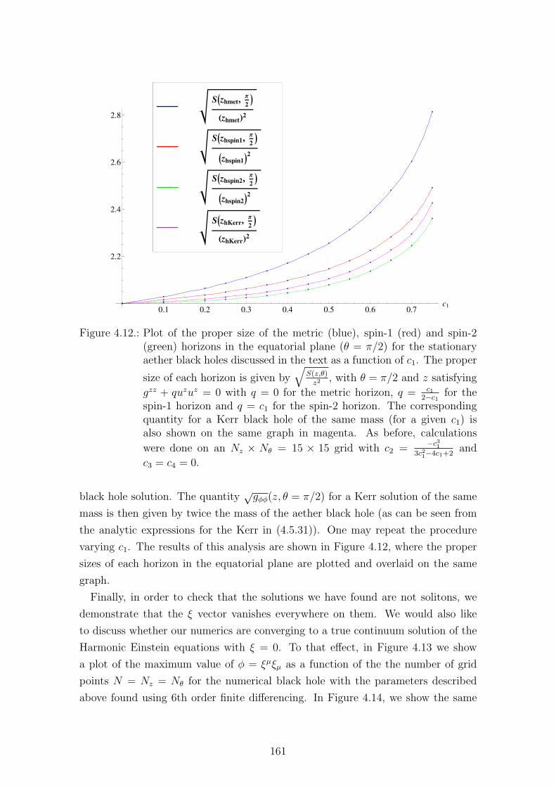
0.1 0.2 0.3 0.4 0.5 0.6 0.7c1

2.2

2.4

2.6

2.8

SIzhKerr,Π

2M

HzhKerrL2

SIzhspin2,Π

2M

Izhspin2M2

SIzhspin1,Π

2M

Izhspin1M2

SIzhmet,Π

2M

HzhmetL2

Figure 4.12.: Plot of the proper size of the metric (blue), spin-1 (red) and spin-2(green) horizons in the equatorial plane (θ = π/2) for the stationaryaether black holes discussed in the text as a function of c1. The proper

size of each horizon is given by√

S(z,θ)z2

, with θ = π/2 and z satisfying

gzz + quzuz = 0 with q = 0 for the metric horizon, q = c12−c1

for thespin-1 horizon and q = c1 for the spin-2 horizon. The correspondingquantity for a Kerr black hole of the same mass (for a given c1) isalso shown on the same graph in magenta. As before, calculations

were done on an Nz × Nθ = 15 × 15 grid with c2 =−c31

3c21−4c1+2and

c3 = c4 = 0.

black hole solution. The quantity√gφφ(z, θ = π/2) for a Kerr solution of the same

mass is then given by twice the mass of the aether black hole (as can be seen from

the analytic expressions for the Kerr in (4.5.31)). One may repeat the procedure

varying c1. The results of this analysis are shown in Figure 4.12, where the proper

sizes of each horizon in the equatorial plane are plotted and overlaid on the same

graph.

Finally, in order to check that the solutions we have found are not solitons, we

demonstrate that the ξ vector vanishes everywhere on them. We would also like

to discuss whether our numerics are converging to a true continuum solution of the

Harmonic Einstein equations with ξ = 0. To that effect, in Figure 4.13 we show

a plot of the maximum value of φ = ξµξµ as a function of the the number of grid

points N = Nz = Nθ for the numerical black hole with the parameters described

above found using 6th order finite differencing. In Figure 4.14, we show the same

161

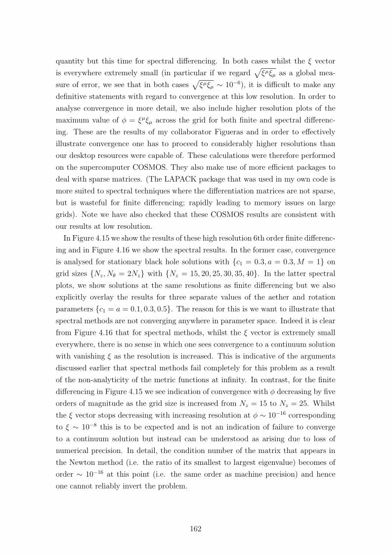
quantity but this time for spectral differencing. In both cases whilst the ξ vector

is everywhere extremely small (in particular if we regard√ξµξµ as a global mea-

sure of error, we see that in both cases√ξµξµ ∼ 10−6), it is difficult to make any

definitive statements with regard to convergence at this low resolution. In order to

analyse convergence in more detail, we also include higher resolution plots of the

maximum value of φ = ξµξµ across the grid for both finite and spectral differenc-

ing. These are the results of my collaborator Figueras and in order to effectively

illustrate convergence one has to proceed to considerably higher resolutions than

our desktop resources were capable of. These calculations were therefore performed

on the supercomputer COSMOS. They also make use of more efficient packages to

deal with sparse matrices. (The LAPACK package that was used in my own code is

more suited to spectral techniques where the differentiation matrices are not sparse,

but is wasteful for finite differencing; rapidly leading to memory issues on large

grids). Note we have also checked that these COSMOS results are consistent with

our results at low resolution.

In Figure 4.15 we show the results of these high resolution 6th order finite differenc-

ing and in Figure 4.16 we show the spectral results. In the former case, convergence

is analysed for stationary black hole solutions with c1 = 0.3, a = 0.3,M = 1 on

grid sizes Nz, Nθ = 2Nz with Nz = 15, 20, 25, 30, 35, 40. In the latter spectral

plots, we show solutions at the same resolutions as finite differencing but we also

explicitly overlay the results for three separate values of the aether and rotation

parameters c1 = a = 0.1, 0.3, 0.5. The reason for this is we want to illustrate that

spectral methods are not converging anywhere in parameter space. Indeed it is clear

from Figure 4.16 that for spectral methods, whilst the ξ vector is extremely small

everywhere, there is no sense in which one sees convergence to a continuum solution

with vanishing ξ as the resolution is increased. This is indicative of the arguments

discussed earlier that spectral methods fail completely for this problem as a result

of the non-analyticity of the metric functions at infinity. In contrast, for the finite

differencing in Figure 4.15 we see indication of convergence with φ decreasing by five

orders of magnitude as the grid size is increased from Nz = 15 to Nz = 25. Whilst

the ξ vector stops decreasing with increasing resolution at φ ∼ 10−16 corresponding

to ξ ∼ 10−8 this is to be expected and is not an indication of failure to converge

to a continuum solution but instead can be understood as arising due to loss of

numerical precision. In detail, the condition number of the matrix that appears in

the Newton method (i.e. the ratio of its smallest to largest eigenvalue) becomes of

order ∼ 10−16 at this point (i.e. the same order as machine precision) and hence

one cannot reliably invert the problem.

162

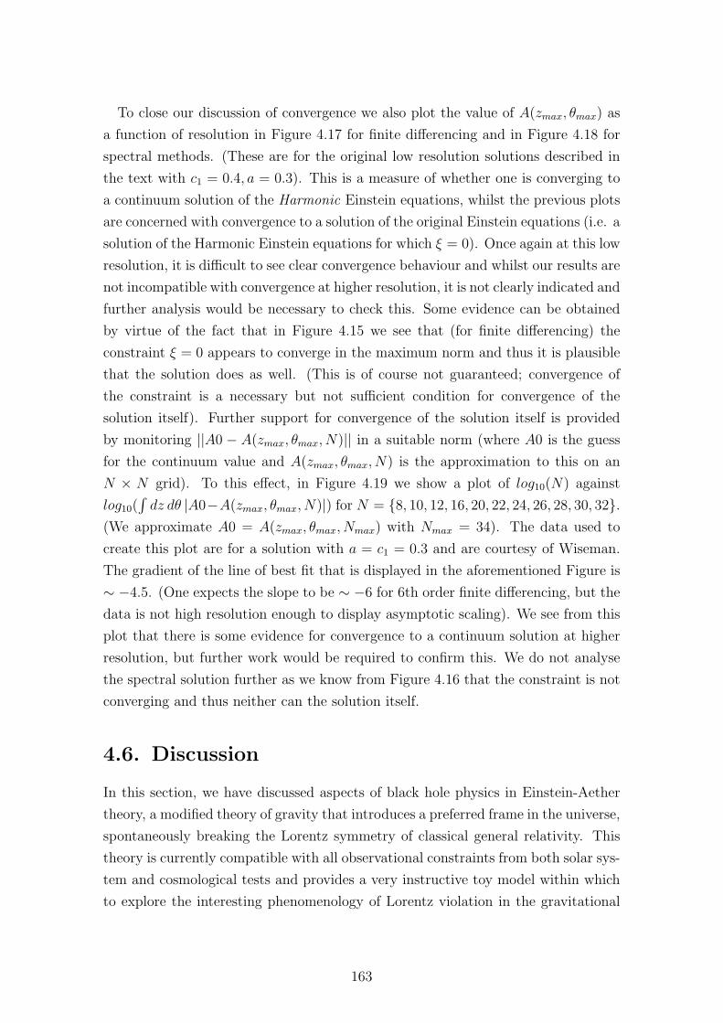
To close our discussion of convergence we also plot the value of A(zmax, θmax) as

a function of resolution in Figure 4.17 for finite differencing and in Figure 4.18 for

spectral methods. (These are for the original low resolution solutions described in

the text with c1 = 0.4, a = 0.3). This is a measure of whether one is converging to

a continuum solution of the Harmonic Einstein equations, whilst the previous plots

are concerned with convergence to a solution of the original Einstein equations (i.e. a

solution of the Harmonic Einstein equations for which ξ = 0). Once again at this low

resolution, it is difficult to see clear convergence behaviour and whilst our results are

not incompatible with convergence at higher resolution, it is not clearly indicated and

further analysis would be necessary to check this. Some evidence can be obtained

by virtue of the fact that in Figure 4.15 we see that (for finite differencing) the

constraint ξ = 0 appears to converge in the maximum norm and thus it is plausible

that the solution does as well. (This is of course not guaranteed; convergence of

the constraint is a necessary but not sufficient condition for convergence of the

solution itself). Further support for convergence of the solution itself is provided

by monitoring ||A0 − A(zmax, θmax, N)|| in a suitable norm (where A0 is the guess

for the continuum value and A(zmax, θmax, N) is the approximation to this on an

N × N grid). To this effect, in Figure 4.19 we show a plot of log10(N) against

log10(∫dz dθ |A0−A(zmax, θmax, N)|) for N = 8, 10, 12, 16, 20, 22, 24, 26, 28, 30, 32.

(We approximate A0 = A(zmax, θmax, Nmax) with Nmax = 34). The data used to

create this plot are for a solution with a = c1 = 0.3 and are courtesy of Wiseman.

The gradient of the line of best fit that is displayed in the aforementioned Figure is

∼ −4.5. (One expects the slope to be ∼ −6 for 6th order finite differencing, but the

data is not high resolution enough to display asymptotic scaling). We see from this

plot that there is some evidence for convergence to a continuum solution at higher

resolution, but further work would be required to confirm this. We do not analyse

the spectral solution further as we know from Figure 4.16 that the constraint is not

converging and thus neither can the solution itself.

4.6. Discussion

In this section, we have discussed aspects of black hole physics in Einstein-Aether

theory, a modified theory of gravity that introduces a preferred frame in the universe,

spontaneously breaking the Lorentz symmetry of classical general relativity. This

theory is currently compatible with all observational constraints from both solar sys-

tem and cosmological tests and provides a very instructive toy model within which

to explore the interesting phenomenology of Lorentz violation in the gravitational

163

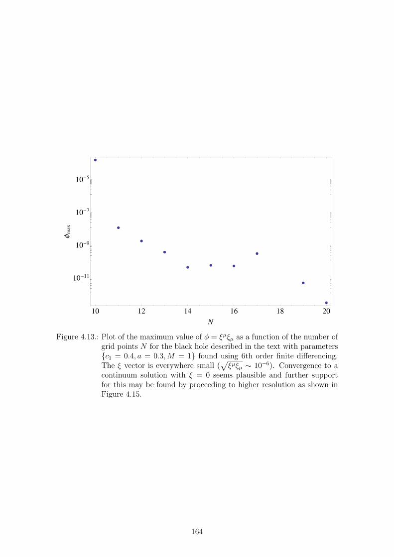
10 12 14 16 18 20

10-11

10-9

10-7

10-5

N

Φm

ax

Figure 4.13.: Plot of the maximum value of φ = ξµξµ as a function of the number ofgrid points N for the black hole described in the text with parametersc1 = 0.4, a = 0.3,M = 1 found using 6th order finite differencing.The ξ vector is everywhere small (

√ξµξµ ∼ 10−6). Convergence to a

continuum solution with ξ = 0 seems plausible and further supportfor this may be found by proceeding to higher resolution as shown inFigure 4.15.

164

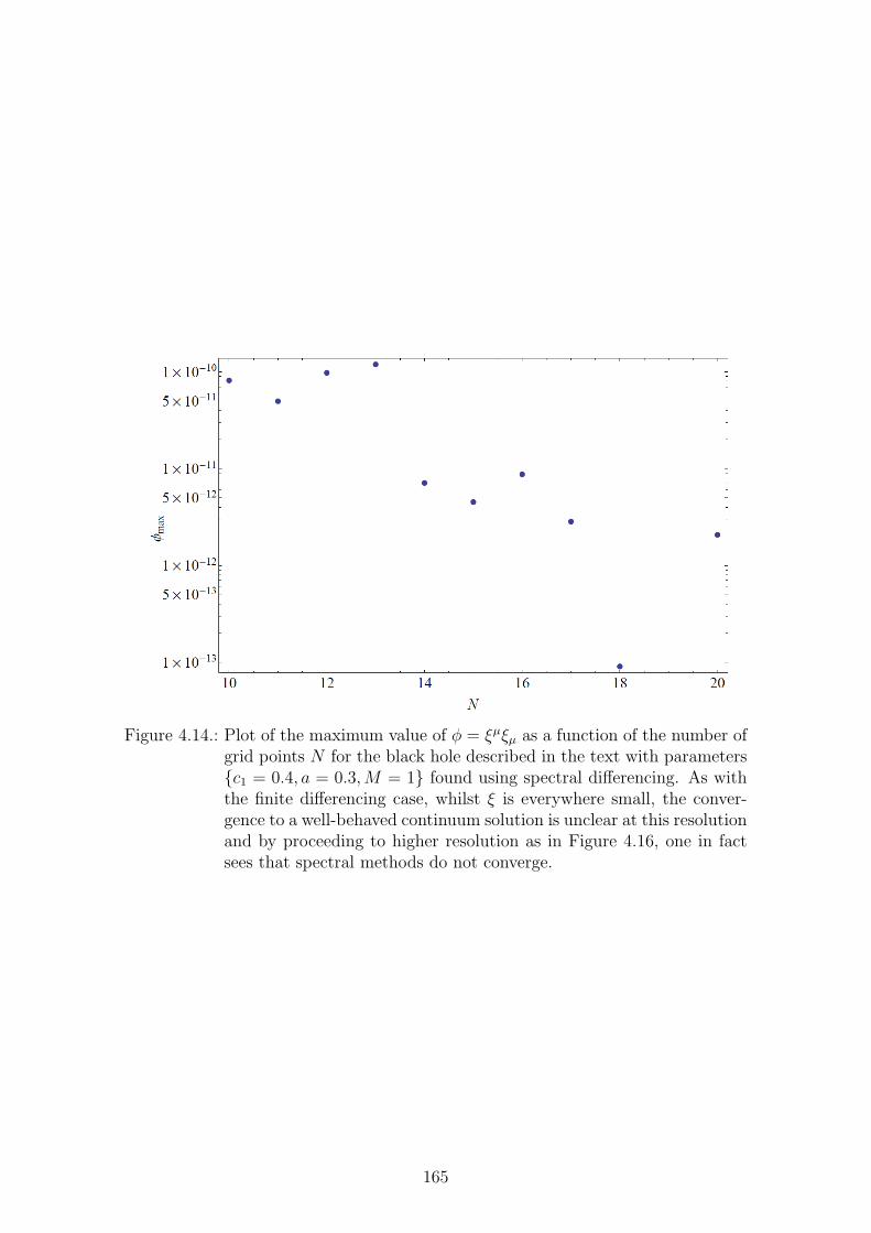
Figure 4.14.: Plot of the maximum value of φ = ξµξµ as a function of the number ofgrid points N for the black hole described in the text with parametersc1 = 0.4, a = 0.3,M = 1 found using spectral differencing. As withthe finite differencing case, whilst ξ is everywhere small, the conver-gence to a well-behaved continuum solution is unclear at this resolutionand by proceeding to higher resolution as in Figure 4.16, one in factsees that spectral methods do not converge.

165

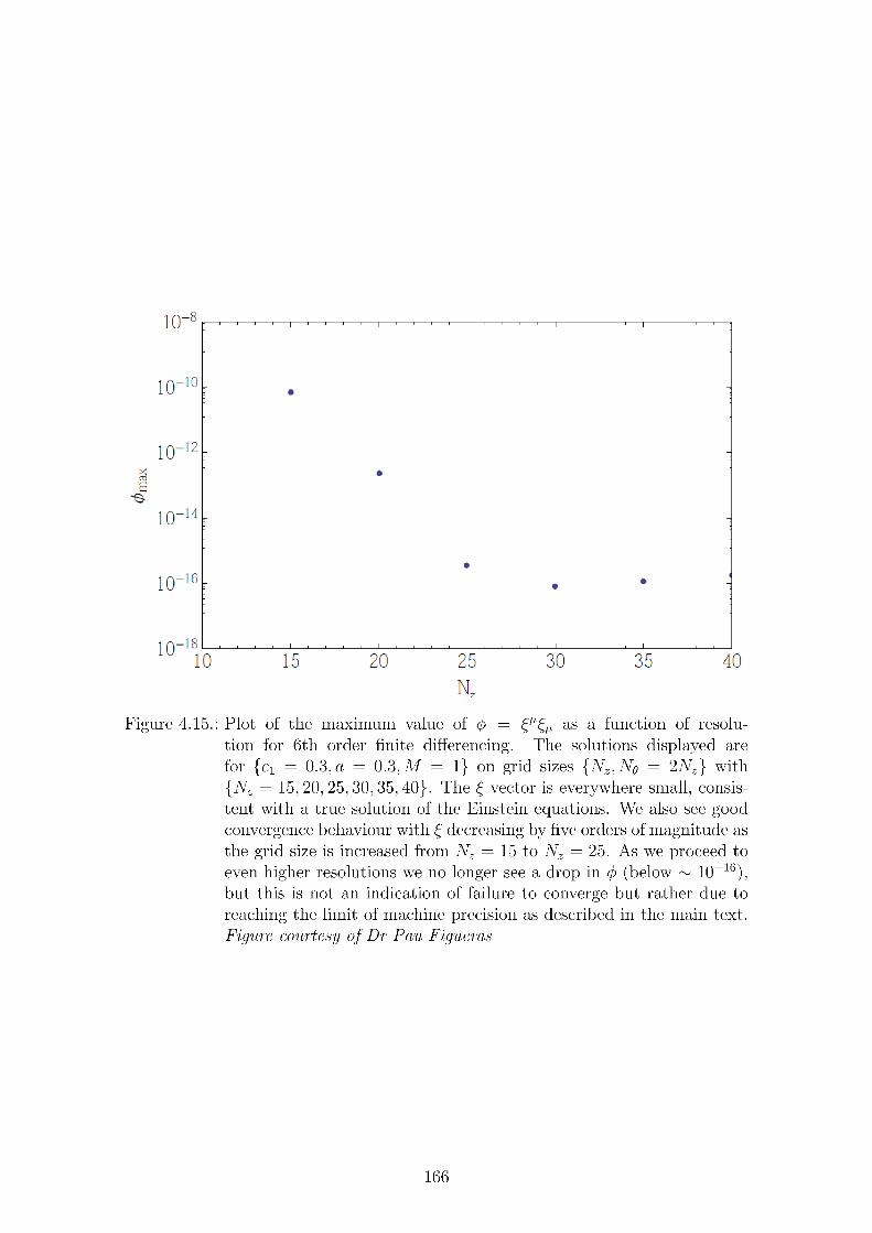
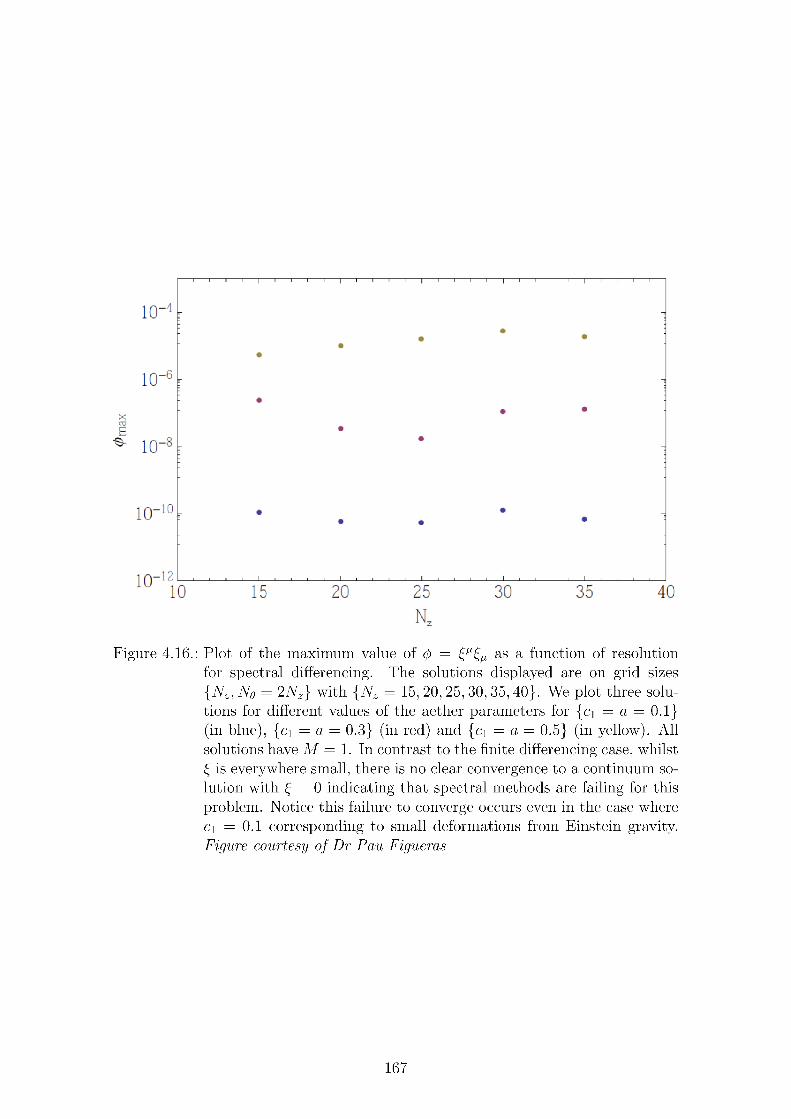
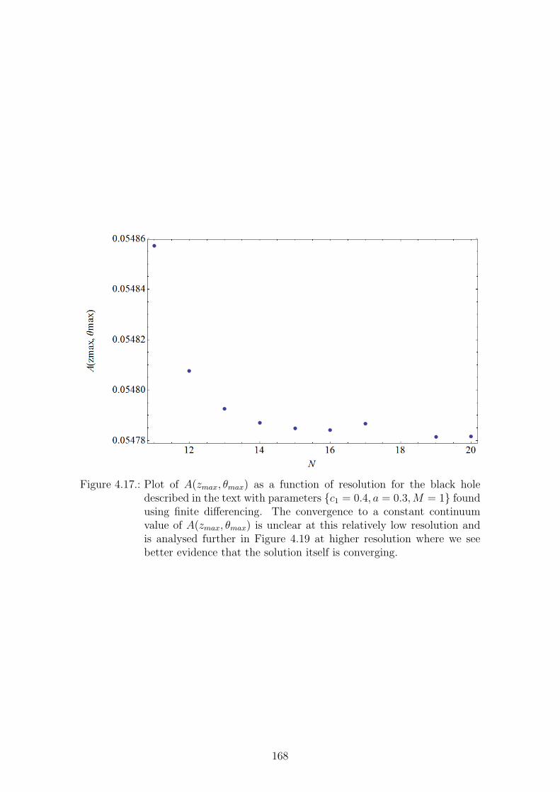
Figure 4.17.: Plot of A(zmax, θmax) as a function of resolution for the black holedescribed in the text with parameters c1 = 0.4, a = 0.3,M = 1 foundusing finite differencing. The convergence to a constant continuumvalue of A(zmax, θmax) is unclear at this relatively low resolution andis analysed further in Figure 4.19 at higher resolution where we seebetter evidence that the solution itself is converging.

168

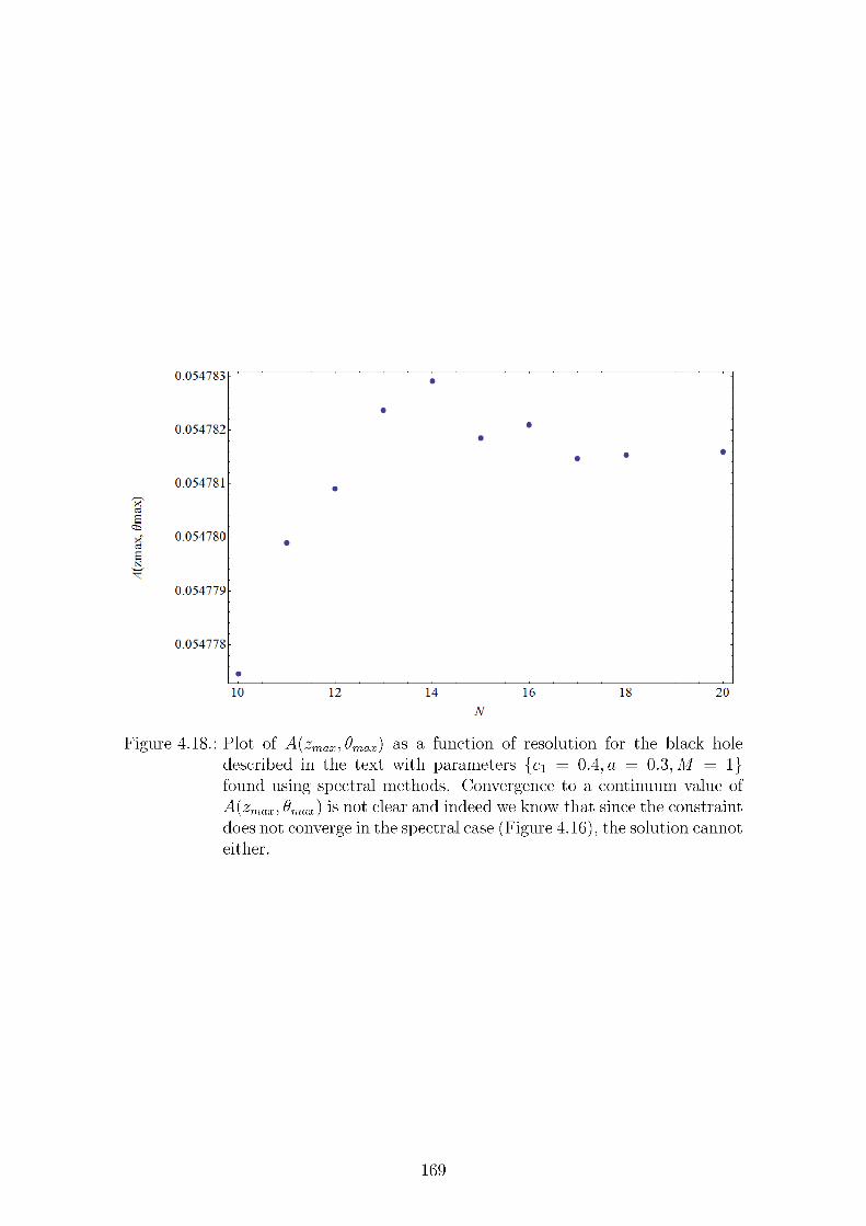
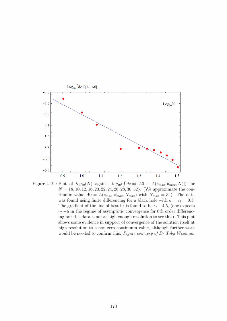
Figure 4.19.: Plot of log10(N) against log10(∫dz dθ |A0 − A(zmax, θmax, N)|) for

N = 8, 10, 12, 16, 20, 22, 24, 26, 28, 30, 32. (We approximate the con-tinuum value A0 = A(zmax, θmax, Nmax) with Nmax = 34). The datawas found using finite differencing for a black hole with a = c1 = 0.3.The gradient of the line of best fit is found to be ∼ −4.5, (one expects∼ −6 in the regime of asymptotic convergence for 6th order differenc-ing but this data is not at high enough resolution to see this). This plotshows some evidence in support of convergence of the solution itself athigh resolution to a non-zero continuum value, although further workwould be needed to confirm this. Figure courtesy of Dr Toby Wiseman

170

sector. As a consequence of the spontaneously broken Lorentz symmetry, the theory

has multiple propagating degrees of freedom, each governed by a different charac-

teristic hypersurface (that it is null with respect to). The notion of a black hole in

such theories is hence quite subtle and in particular must trap all these additional

causal influences together with the more conventional matter influences that couple

directly to the metric gµν itself. Having fixed some definitions, we demonstrated

how to construct spherically symmetric black holes in Einstein-Aether theory us-

ing a modification of the methods of elliptic numerical relativity discussed in 3. In

particular, as a consequence of the layered multi-horizon structure that these black

holes possess, it was necessary to construct numerical solutions interior to the metric

horizon to exhibit their full structure. We therefore posed the Harmonic Einstein

equations on an ingoing slice of the spacetime that extended into the interior of the

black hole. These equations cease to be elliptic in this region (and in fact within an

ergoregion if one exists) and thus the equations we had to solve constitute a mixed

hyperbolic elliptic problem. The technical procedure of solving these equations nev-

ertheless carries over from the elliptic procedures discussed previously in this thesis

with little modification, aside from the prescription of boundary conditions. Whilst

in the fully elliptic case, data is imposed on all interior and asymptotic boundaries

in the problem, in the mixed elliptic hyperbolic case it needs only to be imposed

asymptotically. Moreover, since in the latter case specification of a reference metric

no longer fixes any moduli associated to a solution, these had to be fixed separately

leading to specification of additional conditions at the innermost point of the do-

main (one additional constraint in the static case to fix the mass and two in the

stationary case to fix mass and angular momentum). Within this framework, we

were able to construct static, spherically symmetric black holes in Einstein-Aether

theory, solving the Harmonic Einstein equations by the Newton method and demon-

strating that these solutions were the same as what had previously been found in the

literature using different (shooting) techniques. Furthermore, we were able to extend

our techniques to construct the first examples of stationary, rotating black holes in

Einstein-Aether theory. We performed our calculations using a field redefinition to

make the metric and spin-0 horizons in the theory coincide and regularity at the

spin-0 horizon was hence encoded from the outset by virtue of the fact that smooth-

ness at the metric horizon is guaranteed in our ingoing chart with our boundary

conditions.

There are a number of directions in which the work we have discussed in this

chapter could be extended. In addition to simply providing a more in depth analysis

of the space of stationary solutions in Einstein-Aether theory that we will discuss

171

in a forthcoming publication, it is of interest to explore the horizon structure of the

theory and describe the embeddings of the metric, spin-0, 1 and 2 horizons and study

how their structure varies as a functions of the aether parameters ci. Furthermore, in

the interest of simplicity we restricted our analysis here to the subspace of parameter

space for which c3 = c4 = 0, and it would be interesting to relax this requirement to

investigate whether one finds qualitatively similar solutions in those cases to what we

have found here. It is of course also of interest to explore black holes in the regions

of aether parameter space that are phenomenologically viable. Beyond Einstein-

Aether theory, the techniques we have discussed in this chapter would also be useful

to shed light on the study of black holes in various other theories of modified gravity,

notably Horava-Lifshitz theory and it would be interesting to investigate the phase

space of stationary solutions there, in particular to further investigate the results of

Barausse [210, 221], that suggest there are no slowly rotating solutions common to

both theories. Finally, we note that it would be very interesting to explore in greater

detail the thermodynamics of these black holes, and in particular to investigate the

first law of thermodynamics that is applicable in these static and stationary settings.

172

5. Conclusions and Summary

Since its creation, general relativity has gradually established itself as one of the cor-

nerstones of modern physics. Despite its abstract and highly theoretical beginnings,

drawing on the nascent areas of pure mathematics of the time, (notably differential

geometry), the theory today has remarkably become as significant in applied science

as theoretical physics, having practical applications to satellite and GPS technology.

In theoretical physics, general relativity underlies almost all of modern cosmology

together with large portions of stellar astrophysics as well as serving as a powerful

arena in which to study aspects of fundamental theories of quantum gravity, notably

string and M-theory. It has become the pinnacle of elegance in modern physics to

which we aspire to and to which we compare new gravitational theories that attempt

to go beyond Einstein’s theory. In this thesis we have studied a variety of different

aspects of relativity in four and higher dimensions and in particular, we have high-

lighted how numerical relativity especially is invaluable in studying phenomena as

diverse as a phase transitions in condensed matter and Lorentz violation in mod-

ified gravity. We note though that despite discussing a broad and exotic range of

topics, we have in truth barely scratched the surface of the enormous field that is

numerical relativity, restricting our discussion to stationary systems and remaining

almost silent on the fascinating and complex problem of dynamical gravity.

In chapter 1, we introduced the prerequisite background theory of relevance to

this thesis, discussing in particular various important aspects of the theory of black

holes which to a large extent served as the unifying theme throughout our work. We

reviewed the various uniqueness and ‘no-hair’ theorems that constrain solutions in

four and higher dimensions where it became clear that whilst black holes in D = 4

are rather well-behaved objects, their higher dimensional cousins have no such man-

ners highlighting the importance of numerics in higher dimensional gravity. Having

introduced aspects of black hole theory, we went on to discuss the remarkable topic

of black hole thermodynamics and reviewed gravitational aspects of holography. In

particular, we explained how one can study very complicated (and strongly coupled)

field theories at finite temperature and density by simple dual geometries describ-

ing hairy black holes, where heuristically the Hawking temperature of the horizon

173

accounts for the temperature of the field theory, and the hair for the matter con-

tent of the theory. The second part of the introduction introduced elliptic methods

for static numerical relativity and the all important Harmonic Einstein equation.

Without gauge fixing, the Einstein equations Rµν = 0 are of indefinite signature

which can be inconvenient for numerics. By following DeTurck, and adding −∇(µξν)

to this, one can recast the Euclidean Einstein equations as an elliptic boundary

value problem. The remainder of this section consisted of a detailed treatment of

the boundary conditions appropriate to this elliptic problem together with an ex-

planation of how subject to choosing boundary conditions compatible with ξµ = 0

one is likely (and sometimes guaranteed by maximum principles) to find solutions

of the original Einstein equations. We then outlined two numerical algorithms to

solve the Harmonic Einstein equation, namely Ricci flow and the Newton method.

We ended the introduction with an overview of Einstein-Aether theory, a modified

theory of gravity that spontaneously breaks Lorentz symmetry by the inclusion of a

dynamical timelike vector field of unit norm. We presented the action and discussed

various non-trivial field redefinitions and transformations of the parameters defin-

ing the theory c1, c2, c3, c4 that can be used to simplify the equations of motion.

We then briefly discussed constraints on the theory from a number of solar system

and cosmological tests and finally presented a detailed analysis of the propagating

degrees of freedom in the theory. The latter analysis is our own and does not ap-

pear in the literature and in particular used the Harmonic Einstein equations to

compute the effective metrics governing each of the wavemodes in the theory which

were later used in our discussion of Einstein-Aether black holes in the final chapter

of this thesis.

In chapter 2 we discussed our first and simplest application of numerical relativ-

ity, developing a holographic description of bosonic fractionalisation transitions in

condensed matter physics. We began with some motivation for the subject, intro-

ducing the concept of fractionalised phases of matter where composite particles split

apart into their gauge charged constituents and argued that this is dual in gravity

to geometries where electric flux is sourced by an electrically charged horizon as

opposed to bulk charged matter. The gravitational description of fractionalisation

then amounts to studying transitions between electrically charged black holes and

neutral black holes supporting charged scalar hair. We considered a simple class of

theories consisting of gravity and a Maxwell field together with a real and charged

scalar and used a simple planar, static ansatz to construct black hole solutions. On

this ansatz, the Einstein equations reduced to ODEs and the problem of construct-

ing our solutions was framed as a shooting problem where T = 0 IR geometries

174

describing fractionalised, cohesive or partially fractionalised states of matter had to

be connected to a universal AdS4 asymptotic structure. We constructed one pa-

rameter families of each class of solutions and exhibited transitions between them,

arguing that the existence or non-existence of a fractionalisation transition can be

attributed to the IR behaviour of the real scalar which controls the Maxwell cou-

pling. In cases where this coupling vanishes, charged matter is unable to source

any flux, meaning a cohesive phase becomes impossible and full fractionalisation is

the only possibility. Although the analysis here was restricted to T = 0, we made

some comments on finite temperature and in the light of our newfound insights

studied also M-theory. We explained the absence of a T = 0 fractionalised phase

there as being a consequence of the finiteness of the effective gauge coupling in this

theory in the IR. There are various interesting directions in which this work could

be taken further: It would be of interest to study fractionalisation in a more general

ansatz than (2.2.10), in particular to allow for the presence of spatial modulation

and stripes. This problem is also of general interest in the context of this thesis as

the elliptic PDE methods explored here provide a natural framework to solve the

equations that result in such cases. It would also be of interest to study the order

of such fractionalisation transitions. A more open ended and complex problem is

to shed light on a possible field theory order parameter for fractionalisation and its

relation to entanglement entropy [230].

In chapter 3 we discussed the stationary generalisation of the elliptic PDE methods

of the introductory chapter of this thesis. Unlike for static spacetimes where there

exists a well defined analytic continuation to a smooth real Riemannian geometry, in

stationary situations the problem must be treated directly in Lorentzian signature.

We argued that for stationary spacetimes with globally timelike Killing vector, the

Harmonic Einstein equations are straightforwardly elliptic. In the presence of hori-

zons and ergo-regions however the situation is less obvious and the analysis of such

situations constituted the bulk of this chapter. Motivated by the Rigidity Theorem,

we specialised to a class of stationary black hole spacetimes, discussed previously

by Harmark [207]. The metric ansatz we considered geometrically describes a fi-

bration of the Killing directions over a base manifold and we then argued that the

Harmonic Einstein equations truncate to an elliptic system on this ansatz subject

to the assumption that the base space manifold is Riemannian - a condition we

showed to be satisfied in D = 4 by the Kerr solution. The Killing horizons and

axes of symmetry constitute boundaries for this elliptic problem and we determined

the necessary conditions that must be imposed there to obtain a regular solution.

Whilst we did not explicitly consider numerical applications of this technology here

175

(examples may be found in [1]), related methods were used in the closing chapter

on Einstein-Aether theory.

In the final chapter of this thesis, 4, we turned to a discussion of black holes

in Einstein-Aether theory. As a consequence of the spontaneously broken Lorentz

symmetry in this theory, there exist propagating wave modes of different speeds

(that each in general differ from the metric speed of light) and it is hence some-

what unclear what is meant by a ‘black hole’ in such situations. Following Jacobson

[150], we argued that the notion is well defined in the sense that aether black holes

have multiple horizons each trapping a wavemode of different spin and that a true

black hole must possess a ‘universal’ outer horizon that traps the fastest of these

modes. With these definitions we demonstrated that one can indeed construct both

spherically symmetric and stationary aether black holes. In order to numerically

construct these solutions, we used a generalisation of the numerical techniques of

chapter 3. In particular, since aether black holes possess multiple horizons, we were

required to develop the solution interior to the metric horizon to exhibit their full

structure. In these regions however, the Harmonic Einstein equations ceased to be

elliptic and we hence framed the problem as a mixed elliptic-hyperbolic PDE prob-

lem, specifying in detail the new boundary conditions for the system. (In particular,

unlike in the formalism of chapter 3, no data must now be imposed at the innermost

points of the PDE domain). We were then able to solve the resulting PDE system

by implementing the Newton method. With this setup we were able to construct

the same spherically symmetric aether black holes that had previously been found in

the literature by shooting techniques and moreover were able to construct the first

examples of general stationary black holes in Einstein-Aether theory. We closed

our discussion by initiating an analysis of the physics of such stationary solutions

looking at the relative sizes of the spin-0, 1 and 2 horizons in the equatorial plane

as a function of the aether parameter c1 and comparing with the Kerr solution of

the same mass. As further work it would be very interesting to develop the physics

of these solutions further, in particular by studying the structure of the full horizon

embeddings (as opposed to simply at the axes and plane of reflection symmetry) as

well as studying in greater depth the full parameter space of stationary solutions

(and in particular intoducing non-zero c3 and c4 parameters). It would also be of

interest to consider applying our new technology to study black holes in related

theories of modified gravity notably Horava-Lifshitz gravity.

176

A. Boundary Conditions for

Horizons and Axes

The procedure of deriving the regularity conditions at an axis or horizon boundary

plays a central role in both static and stationary elliptic numerical relativity and is

the subject of this appendix.

The technique is best illustrated by way of an example. We shall derive the

regularity conditions for a smooth (0, 2) tensor J , which is symmetric with respect

to a vector field R and which generates U(1) orbits with period 2π and fixed action

at some point p. Following the prescription outlined above in the main text, the

tensor is first written in ‘Cartesian coordinates’ (a, b) that do not manifest the

U(1) isometry, but crucially in which the components are C∞ smooth everywhere,

including the fixed point. We then shift to polar coordinates (r, α) adapted to the

symmetry, so that R = ∂/∂α and in which the components do not depend explicitly

on α. In detail, we begin with,

J = N(a, b)da2 +M(a, b)db2 +K(a, b)dadb , (A.0.1)

and now introduce ‘polar coordinates’ r, α that make explicit the U(1) isometry

a = r sinα , b = r cosα , (A.0.2)

where we note once again that ∂∂α

is Killing and r = 0 at the fixed point. The metric

may then be recast in the form

J = r2A(r2)dα2 +B(r2)dr2 + r3C(r2)dr dα , (A.0.3)

where the metric functions A(r2), B(r2), C(r2) are trivially related to those in the

Cartesian coordinates by the chain rule. The isometry conditions,∂A(r2)∂α

= ∂B(r2)∂α

=∂C(r2)

∂α= 0 then translate into conditions on the original metric functionsN(a, b),M(a, b)

and K(a, b) and evaluation of these equations at the origin gives the regularity con-

177

ditions,

N(0, 0) =M(0, 0) , K(0, 0) = 0 , (A.0.4)

which when expressed in terms of the polar metric functions become,

A(0) = B(0) . (A.0.5)

These functions may be written in the form

A(r2(a, b)) = N(a, b)b2

a2 + b2+M(a, b)

a2

a2 + b2−K(a, b)

ab

a2 + b2, (A.0.6)

with similar equations for B(r2(a, b)) and C(r2(a, b)). As a consequence of the

above regularity conditions, we see that these functions are smooth everywhere in

a, b (including at the origin) and since arbitrary fractional powers of (a2 + b2) are

not smooth in a, b at the origin, A(r2), B(r2) and C(r2) must contain no odd powers

of r. Consequently, A(r2), B(r2) and C(r2) are smooth in r2.

To summarise then, the conditions required for smoothness of J everywhere in

polar coordinates are that A,B and C are smooth functions of r2 that satisfy the

regularity condition A(0) = B(0). One may consider the Ricci-DeTurck flow or

Newton method operating on this simple example metric (A.0.1) in ‘Cartesian’ co-

ordinates. Let us also take the reference metric to similarly have the same U(1)

isometry generated by ∂∂α. Then Ricci-DeTurck flow and the Newton method will

act to preserve this isometry. At least for short flow times Ricci-DeTurck flow will

preserve regularity. Let us also assume that the Newton method does too. Then

both algorithms will preserve the regularity conditions deduced above for the ‘Polar’

form of the metric (A.0.3). The important consequence of this is that we may work

directly with the ‘Polar’ form, taking our initial data and reference metric to be

regular, and then this regularity should be preserved by the Ricci-DeTurck flow and

Newton method.

A.1. Regularity and smoothness at a Killing

horizon

A Killing horizon implies the existence of a normal Killing field K, whose isometry

group is , with a fixed point at the bifurcation surface, and whose orbits close on

the future and past horizons. We consider a smooth (0, 2) tensor that is symmetric

178

under K, in a chart adapted to the symmetry which covers the exterior of the

Killing horizon. The fixed point may be regarded as a boundary of this chart, and

we determine regularity conditions on the tensor components there.

We begin in smooth Cartesian coordinates with a (0, 2) tensor, J , written in

components as

J = Nda2 +Mdb2 + Udadb+Qidadxi +Ridbdx

i + Tijdxidxj , (A.1.7)

where i = 1, ..., D − 2. We take a Killing horizon with respect to the Killing vector

K to be located at a = b and a = −b with bifurcation surface a = b = 0. Since J

is smooth at the horizon these component functions are C∞ in the neighbourhood

of the horizon. The horizon Killing symmetry is not manifest in these coordinates

and in analogy with the toy example, we now change to hyperbolic coordinates

a = r sinhκt , b = r coshκt , (A.1.8)

so that K = ∂/∂t and r = 0 is the bifurcation surface, with κ a constant related to

the normalization of K and giving the surface gravity. We write the metric in this

polar form as

J = −r2Adt2 +Bdr2 + r3Cdrdt+ rFidrdxi + r2Gidtdx

i

+Tijdxidxj , (A.1.9)

where the component functions are independent of t. Repeating the analysis outlined

in the toy example one arrives at the conclusion that the functions A,B,C, Fi, Gi, Tij

depend smoothly on r2 and xi, together with the regularity condition

A|r=0 = κ2B|r=0 . (A.1.10)

Thus we see explicitly that the regularity in the chart A.1.9 depends on the normal-

ization of K, and hence the surface gravity. If we take the tensor J to be the metric,

we deduce the regularity conditions on the metric at the Killing horizon. Taking J

to be the Ricci-DeTurck tensor we see the behaviour it will exhibit if it shares the

symmetry and is regular.

179

A.2. Axis of rotation

We now consider a (0, 2) tensor which is symmetric under a Killing field R which

generates rotation about an axis with period 2π. In a chart which manifests the

symmetry the axis is fixed under the U(1) action, and may be regarded as a boundary

for the chart. We determine the regularity conditions for the components in this

chart there. This case is very close to the toy example before.

We begin with a Cartesian line element of the form

J = Nda2 +Mdb2 + Udadb+Qidadxi +Ridbdx

i + Tijdxidxj , (A.2.11)

and the component functions depend smoothly on a, b, xi in the neighbourhood of

the axis which we take to be a = b = 0. We now change to polar coordinates defined

by

a = r sinα , b = r cosα , (A.2.12)

where α has period 2π and R = ∂/∂α and r = 0 is the axis. In these coordinates

we write the tensor as

J = r2Adα2 +Bdr2 + r3Cdrdα + rFidrdxi + r2Gidαdx

i + Tijdxidxj ,

(A.2.13)

and the symmetry is manifest so the metric functions are independent of α. Re-

peating the analysis outlined in the toy example, one finds the metric functions

A,B,C, Fi, Gi, Tij are smooth functions of r2 and xi, together with the regularity

condition

A|r=0 = B|r=0 . (A.2.14)

180

B. Connection Components and

Flow Equations

In this appendix, we give the connection components of the metric 3.4.20 together

with the components of the Ricci tensor and ξ vector. The Christoffel symbols are

given by,

Γijk = Γi

jk +1

2himAAjF

Akm +

1

2himAAkF

Ajm − 1

2himAA

kACj ∂mGAC ,

ΓiAB = −1

2hij∂jGAB ,

ΓABi = −1

2AAjGBCF

Cij +

1

2AAjAC

i ∂jGBC +1

2GAC∂iGBC ,

ΓAij = −AA

mΓmij +

1

2AAkABiF

Bkj +

1

2AAkABjF

Bki + ∂(jA

Ai) +GABAC

(i∂j)GBC

+1

2AAkAB

j ADi ∂kGDB ,

ΓABC =

1

2AAi∂iGBC ,

ΓijA = −1

2hikAB

j ∂kGAB +1

2hikGABF

Bjk , (B.0.1)

where Γijk is the Christoffel connection of the ’submetric’ hij and FA

ij ≡ ∂iAAj −

∂jAAi = ∇iA

Aj − ∇jA

Ai . The covariant derivative in the latter equation, ∇i, is

defined with respect to the connection Γijk of hij (and is metric compatible with

respect to hij). Using these results one finds for the decomposition of the Ricci

tensor,

RAB =1

2hij∇i(∂jGAB)−

1

4GCDhip(∂pGAB)(∂iGCD)

+1

2hijGCD(∂jGCB)(∂iGAD) +

1

4hmihjpGBEGAFF

EmjF

Fip ,

RiA −RABABi =

1

2hjkGAB∇jF

Bik +

1

2hjkFB

ij ∂kGAB +1

4hjmGCDGABF

Bim∂jGCD ,

181

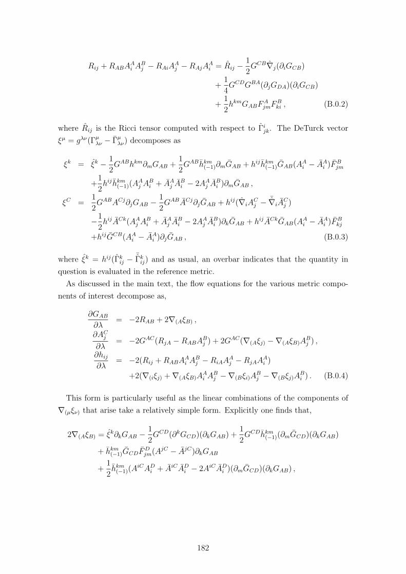
Rij +RABAAi A

Bj −RAiA

Aj −RAjA

Ai = Rij −

1

2GCB∇j(∂iGCB)

+1

4GCDGBA(∂jGDA)(∂iGCB)

+1

2hkmGABF

AjmF

Bki , (B.0.2)

where Rij is the Ricci tensor computed with respect to Γijk. The DeTurck vector

ξµ = gλν(Γµλν − Γµ

λν) decomposes as

ξk = ξk − 1

2GABhkm∂mGAB +

1

2GABhkm(−1)∂mGAB + hijhkm(−1)GAB(A

Ai − AA

i )FBjm

+1

2hijhkm(−1)(A

Aj A

Bi + AA

j ABi − 2AA

j ABi )∂mGAB ,

ξC =1

2GABACj∂jGAB − 1

2GABACj∂jGAB + hij(∇iA

Cj − ¯∇iA

Cj )

−1

2hijACk(AA

j ABi + AA

j ABi − 2AA

j ABi )∂kGAB + hijACkGAB(A

Ai − AA

i )FBkj

+hijGCB(AAi − AA

i )∂jGAB , (B.0.3)

where ξk = hij(Γkij − ¯

Γkij) and as usual, an overbar indicates that the quantity in

question is evaluated in the reference metric.

As discussed in the main text, the flow equations for the various metric compo-

nents of interest decompose as,

∂GAB

∂λ= −2RAB + 2∇(AξB) ,

∂ACj

∂λ= −2GAC(RjA −RABA

Bj ) + 2GAC(∇(Aξj) −∇(AξB)A

Bj ) ,

∂hij∂λ

= −2(Rij +RABAAi A

Bj −RiAA

Aj −RjAA

Ai )

+2(∇(iξj) +∇(AξB)AAi A

Bj −∇(Bξi)A

Bj −∇(Bξj)A

Bi ) . (B.0.4)

This form is particularly useful as the linear combinations of the components of

∇(µξν) that arise take a relatively simple form. Explicitly one finds that,

2∇(AξB) = ξk∂kGAB − 1

2GCD(∂kGCD)(∂kGAB) +

1

2GCDhkm(−1)(∂mGCD)(∂kGAB)

+ hkm(−1)GCDFDjm(A

jC − AjC)∂kGAB

+1

2hkm(−1)(A

iCADi + AiCAD

i − 2AiCADi )(∂mGCD)(∂kGAB) ,

182

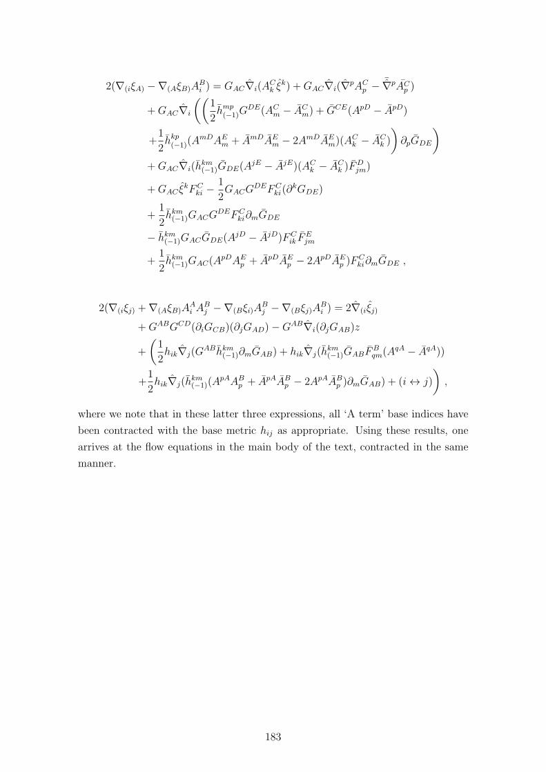
2(∇(iξA) −∇(AξB)ABi ) = GAC∇i(A

Ck ξ

k) +GAC∇i(∇pACp − ¯∇pAC

p )

+GAC∇i

((1

2hmp(−1)G

DE(ACm − AC

m) + GCE(ApD − ApD)

+1

2hkp(−1)(A

mDAEm + AmDAE

m − 2AmDAEm)(A

Ck − AC

k )

)

∂pGDE

)

+GAC∇i(hkm(−1)GDE(A

jE − AjE)(ACk − AC

k )FDjm)

+GAC ξkFC

ki −1

2GACG

DEFCki(∂

kGDE)

+1

2hkm(−1)GACG

DEFCki∂mGDE

− hkm(−1)GACGDE(AjD − AjD)FC

ik FEjm

+1

2hkm(−1)GAC(A

pDAEp + ApDAE

p − 2ApDAEp )F

Cki∂mGDE ,

2(∇(iξj) +∇(AξB)AAi A

Bj −∇(Bξi)A

Bj −∇(Bξj)A

Bi ) = 2∇(iξj)

+GABGCD(∂iGCB)(∂jGAD)−GAB∇i(∂jGAB)z

+

(1

2hik∇j(G

ABhkm(−1)∂mGAB) + hik∇j(hkm(−1)GABF

Bqm(A

qA − AqA))

+1

2hik∇j(h

km(−1)(A

pAABp + ApAAB

p − 2ApAABp )∂mGAB) + (i↔ j)

)

,

where we note that in these latter three expressions, all ‘A term’ base indices have

been contracted with the base metric hij as appropriate. Using these results, one

arrives at the flow equations in the main body of the text, contracted in the same

manner.

183

Bibliography

[1] A. Adam, S. Kitchen, and T. Wiseman, A numerical approach to finding

general stationary vacuum black holes, Class.Quant.Grav. 29 (2012) 165002,

[arXiv:1105.6347].

[2] A. Adam, B. Crampton, J. Sonner, and B. Withers, Bosonic

Fractionalisation Transitions, JHEP 1301 (2013) 127, [arXiv:1208.3199].

[3] L. Lehner, Numerical relativity: A Review, Class.Quant.Grav. 18 (2001)

R25–R86, [gr-qc/0106072].

[4] M. D. Duez, Numerical relativity confronts compact neutron star binaries: a

review and status report, Class.Quant.Grav. 27 (2010) 114002,

[arXiv:0912.3529].

[5] J. A. Font, Numerical hydrodynamics and magnetohydrodynamics in general

relativity, Living Rev.Rel. 11 (2007) 7.

[6] T. Piran, Numerical relativity from gravitational radiation to cosmology, .

PRINT-86-1277 (HEBREW), C86-07-06.

[7] S. A. Hartnoll, Lectures on holographic methods for condensed matter

physics, Class. Quant. Grav. 26 (2009) 224002, [arXiv:0903.3246].

[8] S. A. Hartnoll, Horizons, holography and condensed matter,

arXiv:1106.4324.

[9] S. Sachdev, Condensed Matter and AdS/CFT, Lect.Notes Phys. 828 (2011)

273–311, [arXiv:1002.2947].

[10] C. P. Herzog, Lectures on Holographic Superfluidity and Superconductivity,

J.Phys. A42 (2009) 343001, [arXiv:0904.1975].

[11] J. McGreevy, Holographic duality with a view toward many-body physics,

Adv.High Energy Phys. 2010 (2010) 723105, [arXiv:0909.0518].

184

[12] N. Iizuka, T. Okuda, and J. Polchinski, Matrix Models for the Black Hole

Information Paradox, JHEP 1002 (2010) 073, [arXiv:0808.0530].

[13] N. Iizuka and J. Polchinski, A Matrix Model for Black Hole Thermalization,

JHEP 0810 (2008) 028, [arXiv:0801.3657].

[14] D. N. Kabat, G. Lifschytz, and D. A. Lowe, Black hole thermodynamics from

calculations in strongly coupled gauge theory, Int.J.Mod.Phys. A16 (2001)

856–865, [hep-th/0007051].

[15] D. N. Kabat, G. Lifschytz, and D. A. Lowe, Black hole entropy from

nonperturbative gauge theory, Phys.Rev. D64 (2001) 124015,

[hep-th/0105171].

[16] S. Catterall and T. Wiseman, Towards lattice simulation of the gauge theory

duals to black holes and hot strings, JHEP 0712 (2007) 104,

[arXiv:0706.3518].

[17] G. ’t Hooft, A Planar Diagram Theory for Strong Interactions, Nucl.Phys.

B72 (1974) 461.

[18] J. M. Maldacena, The Large N limit of superconformal field theories and

supergravity, AIP Conf.Proc. 484 (1999) 51–63.

[19] D. M. DeTurck, Deforming metrics in the direction of their Ricci tensors, J.

Differ. Geom. 18 (1983) 157–62.

[20] M. Headrick and T. Wiseman, Ricci flow and black holes, Class. Quant.

Grav. 23 (2006) 6683–6708, [hep-th/0606086].

[21] M. Headrick, S. Kitchen, and T. Wiseman, A new approach to static

numerical relativity, and its application to Kaluza-Klein black holes, Class.

Quant. Grav. 27 (2010) 035002, [arXiv:0905.1822].

[22] T. Jacobson and D. Mattingly, Gravity with a dynamical preferred frame,

Phys.Rev. D64 (2001) 024028, [gr-qc/0007031].

[23] D. Mattingly and T. Jacobson, Relativistic gravity with a dynamical preferred

frame, gr-qc/0112012.

[24] T. Jacobson, Einstein-aether gravity: A Status report, PoS QG-PH (2007)

020, [arXiv:0801.1547].

185

[25] A. Mueller, Experimental Evidence of Black Holes, PoS P2GC (2006) 017,

[astro-ph/0701228].

[26] M. Cavaglia, Black hole and brane production in TeV gravity: A review, Int.

J. Mod. Phys. A18 (2003) 1843–1882, [hep-ph/0210296].

[27] G. L. Landsberg, Black Holes at Future Colliders and Beyond, J.Phys. G32

(2006) R337–R365, [hep-ph/0607297].

[28] G. Landsberg, Out-of-this-world physics: Black holes at future colliders.

proceedings of the space telescope science institute symposium, pages 21-45,

2007.

[29] Y. V. Kovchegov, AdS/CFT applications to relativistic heavy ion collisions:

a brief review, Rept.Prog.Phys. 75 (2012) 124301, [arXiv:1112.5403].

[30] J. Casalderrey-Solana, H. Liu, D. Mateos, K. Rajagopal, and U. A.

Wiedemann, Gauge/String Duality, Hot QCD and Heavy Ion Collisions,

arXiv:1101.0618.

[31] S. S. Gubser, The gauge-string duality and heavy ion collisions,

arXiv:1103.3636.

[32] O. DeWolfe, S. S. Gubser, C. Rosen, and D. Teaney, Heavy ions and string

theory, arXiv:1304.7794.

[33] E. Poisson, A Relativist’s Toolkit : The Mathematics of Black Hole

Mechanics. Cambridge University Press, 2004.

[34] K. Skenderis, Lecture notes on holographic renormalization,

Class.Quant.Grav. 19 (2002) 5849–5876, [hep-th/0209067].

[35] R. M. Wald, General relativity. University of Chicago Press, 1984.

[36] S. Hawking and G. Ellis, The Large Scale Structure of Space-Time.

Cambridge University Press, 1973.

[37] P. O. Mazur, Black hole uniqueness theorems, hep-th/0101012.

[38] D. Robinson, Four decades of black holes uniqueness theorems - The Kerr

spacetime: rotating black holes in general relativity pg.115-143, eds. DL

Wiltshire, M Visser and S M Scott, 2004.

186

[39] R. Emparan and H. S. Reall, Black Holes in Higher Dimensions, Living Rev.

Rel. 11 (2008) 6, [arXiv:0801.3471].

[40] E. by David L. Wiltshire, M. Visser, and S. M. Scott, The Kerr Spacetime:

Rotating Black Holes in General Relativity. Cambridge University Press,

2009.

[41] D. Robinson, Uniqueness of the Kerr black hole, Phys.Rev.Lett. 34 (1975)

905–906.

[42] P. Mazur, Proof of uniqueness of the Kerr-Newman black hole solution,

J.Phys. A15 (1982) 3173–3180.

[43] N. Mavromatos, Eluding the no hair conjecture for black holes,

gr-qc/9606008.

[44] R. Emparan and H. S. Reall, A rotating black ring in five dimensions, Phys.

Rev. Lett. 88 (2002) 101101, [hep-th/0110260].

[45] R. Emparan and H. S. Reall, Black rings, Class. Quant. Grav. 23 (2006)

R169, [hep-th/0608012].

[46] P. T. Chrusciel and R. M. Wald, On the topology of stationary black holes,

Class. Quant. Grav. 11 (1994) L147–L152, [gr-qc/9410004].

[47] J. Stewart, Advanced General Relativity. Cambridge University Press, 1991.

[48] G. Birkhoff, Relativity and modern physics, harvard university press, 1923.

[49] W. Israel, Event horizons in static vacuum space-times, Phys.Rev. 164

(1967) 1776–1779.

[50] G. L. Bunting and A. Masood-ul Alam, Nonexistence of multiple black holes

in asymptotically euclidean static vacuum space-time, General relativity and

gravitation 19 (1987), no. 2 147–154.

[51] F. Tangherlini, Schwarzschild field in n dimensions and the dimensionality of

space problem, Nuovo Cim. 27 (1963) 636–651.

[52] W. Israel, Event horizons in static electrovac space-times,

Commun.Math.Phys. 8 (1968) 245–260.

[53] B. Carter, Black Hole Equilibrium States: II General Theory of Stationary

Black Hole States. Black Holes (proc. 1972 Les Houches Summer School), ed.

B. & C. DeWitt, 1973.

187

[54] S. Hollands, A. Ishibashi, and R. M. Wald, A Higher Dimensional Stationary

Rotating Black Hole Must be Axisymmetric, Commun. Math. Phys. 271

(2007) 699–722, [gr-qc/0605106].

[55] S. Hollands and A. Ishibashi, Black hole uniqueness theorems in higher

dimensional spacetimes, Class.Quant.Grav. 29 (2012) 163001,

[arXiv:1206.1164].

[56] O. J. C. Dias, P. Figueras, R. Monteiro, H. S. Reall, and J. E. Santos, An

instability of higher-dimensional rotating black holes, JHEP 05 (2010) 076,

[arXiv:1001.4527].

[57] O. J. Dias, P. Figueras, R. Monteiro, J. E. Santos, and R. Emparan,

Instability and new phases of higher-dimensional rotating black holes,

Phys.Rev. D80 (2009) 111701, [arXiv:0907.2248].

[58] M. Durkee and H. S. Reall, Perturbations of near-horizon geometries and

instabilities of Myers-Perry black holes, Phys.Rev. D83 (2011) 104044,

[arXiv:1012.4805].

[59] J. M. Bardeen, B. Carter, and S. Hawking, The Four laws of black hole

mechanics, Commun.Math.Phys. 31 (1973) 161–170.

[60] A. Ashtekar and B. Krishnan, Isolated and dynamical horizons and their

applications, Living Rev.Rel. 7 (2004) 10, [gr-qc/0407042].

[61] A. Ashtekar and B. Krishnan, Dynamical horizons and their properties,

Phys.Rev. D68 (2003) 104030, [gr-qc/0308033].

[62] R. M. Wald, The thermodynamics of black holes, gr-qc/9912119.

[63] S. Hawking, Particle Creation by Black Holes, Commun.Math.Phys. 43

(1975) 199–220.

[64] J. D. Bekenstein, Black holes and entropy, Phys.Rev. D7 (1973) 2333–2346.

[65] A. Strominger and C. Vafa, Microscopic origin of the Bekenstein-Hawking

entropy, Phys.Lett. B379 (1996) 99–104, [hep-th/9601029].

[66] G. Gibbons and S. Hawking, Action Integrals and Partition Functions in

Quantum Gravity, Phys.Rev. D15 (1977) 2752–2756.

[67] E. by GW Gibbons and S. Hawking, Euclidean Quantum Gravity. World

Scientific, 1993.

188

[68] B. F. Whiting and J. York, James W., Action Principle and Partition

Function for the Gravitational Field in Black Hole Topologies, Phys.Rev.Lett.

61 (1988) 1336.

[69] J. York, James W., Black hole thermodynamics and the Euclidean Einstein

action, Phys.Rev. D33 (1986) 2092–2099.

[70] S. Hawking and D. N. Page, Thermodynamics of Black Holes in anti-De

Sitter Space, Commun.Math.Phys. 87 (1983) 577.

[71] R. Gregory and R. Laflamme, Black strings and p-branes are unstable, Phys.

Rev. Lett. 70 (1993) 2837–2840, [hep-th/9301052].

[72] R. Gregory and R. Laflamme, The Instability of charged black strings and

p-branes, Nucl. Phys. B428 (1994) 399–434, [hep-th/9404071].

[73] B. Kleihaus, J. Kunz, and E. Radu, New nonuniform black string solutions,

hep-th/0603119.

[74] T. Wiseman, Static axisymmetric vacuum solutions and nonuniform black

strings, Class.Quant.Grav. 20 (2003) 1137–1176, [hep-th/0209051].

[75] T. Harmark, V. Niarchos, and N. A. Obers, Instabilities of black strings and

branes, Class. Quant. Grav. 24 (2007) R1–R90, [hep-th/0701022].

[76] L. Lehner and F. Pretorius, Black Strings, Low Viscosity Fluids, and

Violation of Cosmic Censorship, Phys. Rev. Lett. 105 (2010) 101102,

[arXiv:1006.5960].

[77] H. Kudoh and T. Wiseman, Connecting black holes and black strings,

Phys.Rev.Lett. 94 (2005) 161102, [hep-th/0409111].

[78] B. Kol, Topology change in general relativity and the black-hole black-string

transition, JHEP 10 (2005) 049, [hep-th/0206220].

[79] B. Kol, The Phase Transition between Caged Black Holes and Black Strings -

A Review, Phys. Rept. 422 (2006) 119–165, [hep-th/0411240].

[80] R. P. Kerr, Gravitational field of a spinning mass as an example of

algebraically special metrics, Phys.Rev.Lett. 11 (1963) 237–238.

[81] J. Gariel, M. A. H. MacCallum, G. Marcilhacy, and N. O. Santos, Kerr

Geodesics, the Penrose Process and Jet Collimation by a Black Hole,

gr-qc/0702123.

189

[82] R. C. Myers and M. Perry, Black Holes in Higher Dimensional Space-Times,

Annals Phys. 172 (1986) 304.

[83] R. C. Myers, Myers-Perry black holes, arXiv:1111.1903.

[84] H. Elvang and P. Figueras, Black Saturn, JHEP 0705 (2007) 050,

[hep-th/0701035].

[85] R. Emparan, S. Ohashi, and T. Shiromizu, No-dipole-hair theorem for

higher-dimensional static black holes, Phys.Rev. D82 (2010) 084032,

[arXiv:1007.3847].

[86] M. M. Caldarelli, R. Emparan, and M. J. Rodriguez, Black Rings in

(Anti)-deSitter space, JHEP 0811 (2008) 011, [arXiv:0806.1954].

[87] R. Emparan and P. Figueras, Multi-black rings and the phase diagram of

higher-dimensional black holes, JHEP 1011 (2010) 022, [arXiv:1008.3243].

[88] R. Emparan, T. Harmark, V. Niarchos, N. A. Obers, and M. J. Rodriguez,

The Phase Structure of Higher-Dimensional Black Rings and Black Holes,

JHEP 0710 (2007) 110, [arXiv:0708.2181].

[89] T. Harmark and N. A. Obers, Phases of Kaluza-Klein black holes: A Brief

review, hep-th/0503020.

[90] E. Witten, Anti-de Sitter space and holography, Adv.Theor.Math.Phys. 2

(1998) 253–291, [hep-th/9802150].

[91] S. Gubser, I. R. Klebanov, and A. M. Polyakov, Gauge theory correlators

from noncritical string theory, Phys.Lett. B428 (1998) 105–114,

[hep-th/9802109].

[92] O. Aharony, S. S. Gubser, J. M. Maldacena, H. Ooguri, and Y. Oz, Large N

field theories, string theory and gravity, Phys.Rept. 323 (2000) 183–386,

[hep-th/9905111].

[93] E. D’Hoker and D. Z. Freedman, Supersymmetric gauge theories and the AdS

/ CFT correspondence, hep-th/0201253.

[94] H. Nastase, Introduction to AdS-CFT, arXiv:0712.0689.

[95] G. ’t Hooft, Dimensional reduction in quantum gravity, gr-qc/9310026.

190

[96] R. Bousso, The Holographic principle, Rev.Mod.Phys. 74 (2002) 825–874,

[hep-th/0203101].

[97] S. Kachru, X. Liu, and M. Mulligan, Gravity Duals of Lifshitz-like Fixed

Points, Phys.Rev. D78 (2008) 106005, [arXiv:0808.1725].

[98] S. de Haro, S. N. Solodukhin, and K. Skenderis, Holographic reconstruction

of space-time and renormalization in the AdS / CFT correspondence,

Commun.Math.Phys. 217 (2001) 595–622, [hep-th/0002230].

[99] S. A. Hartnoll, C. P. Herzog, and G. T. Horowitz, Holographic

Superconductors, JHEP 0812 (2008) 015, [arXiv:0810.1563].

[100] J. Wilson, Models of differentially rotating stars, Astrophys. J. 176 (1972)

195–204.

[101] S. Bonazzola and J. Schneider, An exact study of rigidly and rapidly rotating

stars in general relativity with application to the crab pulsar, Astrophys. J.

191 (1974) 273–286.

[102] E. Butterworth and J. Ipser, On the structure and stability of rapidly

rotating fluid bodies in general relativity. i. the numerical method for

computing structure and its application to uniformly rotating homogeneous

bodies, Astrophys. J. 204 (1976) 200–233.

[103] N. Stergioulas, Models of differentially rotating stars, Living Rev. Relativity 6

(2003).

[104] B. Kleihaus and J. Kunz, Static black hole solutions with axial symmetry,

Phys. Rev. Lett. 79 (1997) 1595–1598, [gr-qc/9704060].

[105] B. Kleihaus and J. Kunz, Rotating hairy black holes, Phys. Rev. Lett. 86

(2001) 3704–3707, [gr-qc/0012081].

[106] Y. Morisawa and D. Ida, A boundary value problem for the five-dimensional

stationary rotating black holes, Phys. Rev. D69 (2004) 124005,

[gr-qc/0401100].

[107] S. Hollands and S. Yazadjiev, Uniqueness theorem for 5-dimensional black

holes with two axial Killing fields, Commun. Math. Phys. 283 (2008)

749–768, [arXiv:0707.2775].

191

[108] T. Harmark, Stationary and axisymmetric solutions of higher- dimensional

general relativity, Phys. Rev. D70 (2004) 124002, [hep-th/0408141].

[109] T. Wiseman, Relativistic stars in Randall-Sundrum gravity, Phys. Rev. D65

(2002) 124007, [hep-th/0111057].

[110] S. Donaldson, Some numerical results in complex differential geometry,

arXiv:math.DG/0.

[111] M. Headrick and A. Nassar, Energy functionals for Calabi-Yau metrics,

arXiv:0908.2635.

[112] O. A. Reula, Hyperbolic methods for Einstein’s equations, Living Rev.Rel. 1

(1998) 3.

[113] H.-O. Kreiss and J. Lorenz, Initial-boundary value problems and the

Navier-Stokes equations, vol. 136. Access Online via Elsevier, 1989.

[114] S. Hassani, Mathematical Physics: A modern introduction to its foundation.

Springer, India, 1999.

[115] M. E. Taylor, Partial differential equations I: Basic theory, vol. 1. Springer,

1996.

[116] Y. Foures-Bruhat, Theoreme d’existence pour certains systems d’equations

aux derivees partielles non lineaires, Acta Mathematica 88 (1952) 141.

[117] H. Friedrich, On the hyperbolicity of Einstein’s and other gauge field

equations, Commun. Math. Phys. 100 (1985) 525–543.

[118] D. Garfinkle, Harmonic coordinate method for simulating generic

singularities, Phys. Rev. D65 (2002) 044029, [gr-qc/0110013].

[119] J. Eells and L. Lemaire, Harmonic mappings of Riemannian manifolds,

Amer. J . Math 86 (1964).

[120] J. P. Bourguignon, In Global differential geometry and global analysis

(Berlin, 1979), volume 838 of Lecture notes in Math. pages 42-63. Springer,

Berlin 1981., .

[121] P. Figueras, J. Lucietti, and T. Wiseman, Ricci solitons, Ricci flow, and

strongly coupled CFT in the Schwarzschild Unruh or Boulware vacua,

arXiv:1104.4489.

192

[122] P. M. Topping, Lectures on the Ricci flow. L.M.S. Lecture note series 325

C.U.P., 2006.

[123] T. Oliynyk and E. Woolgar, Asymptotically Flat Ricci Flows, math/0607438.

[124] S. S. Gubser and I. Mitra, The Evolution of unstable black holes in anti-de

Sitter space, JHEP 0108 (2001) 018, [hep-th/0011127].

[125] S. S. Gubser and I. Mitra, Instability of charged black holes in Anti-de Sitter

space, hep-th/0009126.

[126] H. S. Reall, Classical and thermodynamic stability of black branes, Phys.Rev.

D64 (2001) 044005, [hep-th/0104071].

[127] J. J. Friess, S. S. Gubser, and I. Mitra, Counter-examples to the correlated

stability conjecture, Phys.Rev. D72 (2005) 104019, [hep-th/0508220].

[128] D. J. Gross, M. J. Perry, and L. G. Yaffe, Instability of Flat Space at Finite

Temperature, Phys. Rev. D25 (1982) 330–355.

[129] N. E. Mavromatos, On CPT symmetry: Cosmological, quantum gravitational

and other possible violations and their phenomenology, Springer Proc.Phys.

92 (2004) 43–72, [hep-ph/0309221].

[130] G. Amelino-Camelia, The Three perspectives on the quantum gravity problem

and their implications for the fate of Lorentz symmetry, gr-qc/0309054.

[131] T. A. Jacobson, S. Liberati, D. Mattingly, and F. Stecker, New limits on

Planck scale Lorentz violation in QED, Phys.Rev.Lett. 93 (2004) 021101,

[astro-ph/0309681].

[132] V. A. Kostelecky and S. Samuel, Gravitational Phenomenology in Higher

Dimensional Theories and Strings, Phys.Rev. D40 (1989) 1886–1903.

[133] D. Colladay and V. A. Kostelecky, Lorentz violating extension of the

standard model, Phys.Rev. D58 (1998) 116002, [hep-ph/9809521].

[134] D. Mattingly, Modern tests of Lorentz invariance, Living Rev.Rel. 8 (2005) 5,

[gr-qc/0502097].

[135] S. Liberati and L. Maccione, Lorentz Violation: Motivation and new

constraints, Ann.Rev.Nucl.Part.Sci. 59 (2009) 245–267, [arXiv:0906.0681].

193

[136] M. Gasperini, Singularity prevention and broken Lorentz symmetry,

Class.Quant.Grav. 4 (1987) 485–494.

[137] M. Gasperini, Repulsive gravity in the very early universe, Gen.Rel.Grav. 30

(1998) 1703–1709, [gr-qc/9805060].

[138] K. J. Nordtvedt and C. M. Will, Conservation Laws and Preferred Frames in

Relativistic Gravity. II. Experimental Evidence to Rule Out Preferred-Frame

Theories of Gravity, Astrophys.J. 177 (1972) 775–792.

[139] C. M. Will and J. Nordtvedt, Kenneth, Conservation Laws and Preferred

Frames in Relativistic Gravity. I. Preferred-Frame Theories and an Extended

PPN Formalism, Astrophys.J. 177 (1972) 757.

[140] R. W. Hellings and K. Nordtvedt, Vector-Metric Theory of Gravity,

Phys.Rev. D7 (1973) 3593–3602.

[141] M. Clayton and J. Moffat, Dynamical mechanism for varying light velocity as

a solution to cosmological problems, Phys.Lett. B460 (1999) 263–270,

[astro-ph/9812481].

[142] J. Moffat, Variable speed of light cosmology: An Alternative to inflation,

hep-th/0208122.

[143] B. A. Bassett, S. Liberati, C. Molina-Paris, and M. Visser,

Geometrodynamics of variable speed of light cosmologies, Phys.Rev. D62

(2000) 103518, [astro-ph/0001441].

[144] M. Clayton, Causality, shocks and instabilities in vector field models of

Lorentz symmetry breaking, gr-qc/0104103.

[145] N. Arkani-Hamed, H.-C. Cheng, M. A. Luty, and S. Mukohyama, Ghost

condensation and a consistent infrared modification of gravity, JHEP 0405

(2004) 074, [hep-th/0312099].

[146] N. Arkani-Hamed, P. Creminelli, S. Mukohyama, and M. Zaldarriaga, Ghost

inflation, JCAP 0404 (2004) 001, [hep-th/0312100].

[147] V. A. Kostelecky, Gravity, Lorentz violation, and the standard model,

Phys.Rev. D69 (2004) 105009, [hep-th/0312310].

[148] C. M. Will, Theory and Experiment in Gravitational Physics. Cambridge

University Press, 1993.

194

[149] T. Jacobson and D. Mattingly, Einstein-Aether waves, Phys.Rev. D70 (2004)

024003, [gr-qc/0402005].

[150] C. Eling and T. Jacobson, Black Holes in Einstein-Aether Theory,

Class.Quant.Grav. 23 (2006) 5643–5660, [gr-qc/0604088].

[151] B. Z. Foster, Metric redefinitions in Einstein-Aether theory, Phys.Rev. D72

(2005) 044017, [gr-qc/0502066].

[152] E. Barausse, T. Jacobson, and T. P. Sotiriou, Black holes in Einstein-aether

and Horava-Lifshitz gravity, Phys.Rev. D83 (2011) 124043,

[arXiv:1104.2889].

[153] D. Blas, O. Pujolas, and S. Sibiryakov, Comment on ‘Strong coupling in

extended Horava-Lifshitz gravity’, Phys.Lett. B688 (2010) 350–355,

[arXiv:0912.0550].

[154] C. Germani, A. Kehagias, and K. Sfetsos, Relativistic Quantum Gravity at a

Lifshitz Point, JHEP 0909 (2009) 060, [arXiv:0906.1201].

[155] T. Jacobson, Extended Horava gravity and Einstein-aether theory, Phys.Rev.

D81 (2010) 101502, [arXiv:1001.4823].

[156] P. Horava, Quantum Gravity at a Lifshitz Point, Phys.Rev. D79 (2009)

084008, [arXiv:0901.3775].

[157] B. Withers, Einstein-aether as a quantum effective field theory,

Class.Quant.Grav. 26 (2009) 225009, [arXiv:0905.2446].

[158] J. F. Barbero G. and E. J. Villasenor, Lorentz violations and Euclidean

signature metrics, Phys.Rev. D68 (2003) 087501, [gr-qc/0307066].

[159] C. R. Contaldi, T. Wiseman, and B. Withers, TeVeS gets caught on caustics,

Phys.Rev. D78 (2008) 044034, [arXiv:0802.1215].

[160] B. Z. Foster and T. Jacobson, Post-Newtonian parameters and constraints on

Einstein-aether theory, Phys.Rev. D73 (2006) 064015, [gr-qc/0509083].

[161] D. Blas, O. Pujolas, and S. Sibiryakov, Models of non-relativistic quantum

gravity: The Good, the bad and the healthy, JHEP 1104 (2011) 018,

[arXiv:1007.3503].

195

[162] C. Eling and T. Jacobson, Static postNewtonian equivalence of GR and

gravity with a dynamical preferred frame, Phys.Rev. D69 (2004) 064005,

[gr-qc/0310044].

[163] C. M. Will, The Confrontation between general relativity and experiment,

Living Rev.Rel. 9 (2006) 3, [gr-qc/0510072].

[164] J. W. Elliott, G. D. Moore, and H. Stoica, Constraining the new Aether:

Gravitational Cerenkov radiation, JHEP 0508 (2005) 066, [hep-ph/0505211].

[165] G. D. Moore and A. E. Nelson, Lower bound on the propagation speed of

gravity from gravitational Cherenkov radiation, JHEP 0109 (2001) 023,

[hep-ph/0106220].

[166] J. A. Zuntz, P. Ferreira, and T. Zlosnik, Constraining Lorentz violation with

cosmology, Phys.Rev.Lett. 101 (2008) 261102, [arXiv:0808.1824].

[167] B. Li, D. Fonseca Mota, and J. D. Barrow, Detecting a Lorentz-Violating

Field in Cosmology, Phys.Rev. D77 (2008) 024032, [arXiv:0709.4581].

[168] E. A. Lim, Can we see Lorentz-violating vector fields in the CMB?,

Phys.Rev. D71 (2005) 063504, [astro-ph/0407437].

[169] B. Z. Foster, Radiation damping in Einstein-aether theory, Phys.Rev. D73

(2006) 104012, [gr-qc/0602004].

[170] B. Z. Foster, Strong field effects on binary systems in Einstein-aether theory,

Phys.Rev. D76 (2007) 084033, [arXiv:0706.0704].

[171] C. Eling and T. Jacobson, Spherical solutions in Einstein-aether theory:

Static aether and stars, Class.Quant.Grav. 23 (2006) 5625–5642,

[gr-qc/0603058].

[172] C. Eling, T. Jacobson, and M. Coleman Miller, Neutron stars in

Einstein-aether theory, Phys.Rev. D76 (2007) 042003, [arXiv:0705.1565].

[173] S. M. Carroll, T. R. Dulaney, M. I. Gresham, and H. Tam, Instabilities in the

Aether, Phys.Rev. D79 (2009) 065011, [arXiv:0812.1049].

[174] S. A. Hartnoll and L. Huijse, Fractionalization of holographic Fermi surfaces,

arXiv:1111.2606.

[175] L. Huijse and S. Sachdev, Fermi surfaces and gauge-gravity duality, Phys.

Rev. D84 (2011) 026001, [arXiv:1104.5022].

196

[176] N. Iqbal and H. Liu, Luttinger’s Theorem, Superfluid Vortices, and

Holography, arXiv:1112.3671. 21 pages.

[177] S. El-Showk and K. Papadodimas, Emergent Spacetime and Holographic

CFTs, JHEP 1210 (2012) 106, [arXiv:1101.4163].

[178] E. Witten, Anti-de Sitter space, thermal phase transition, and confinement in

gauge theories, Adv.Theor.Math.Phys. 2 (1998) 505–532, [hep-th/9803131].

[179] T. Faulkner and N. Iqbal, Friedel oscillations and horizon charge in 1D

holographic liquids, arXiv:1207.4208.

[180] V. G. M. Puletti, S. Nowling, L. Thorlacius, and T. Zingg, Holographic

metals at finite temperature, JHEP 01 (2011) 117, [arXiv:1011.6261].

[181] E. D’Hoker and P. Kraus, Charge Expulsion from Black Brane Horizons, and

Holographic Quantum Criticality in the Plane, arXiv:1202.2085. 37 pages

v2: reference added and cosmetic improvements.

[182] S. A. Hartnoll and E. Shaghoulian, Spectral weight in holographic scaling

geometries, arXiv:1203.4236.

[183] S. A. Hartnoll and A. Tavanfar, Electron stars for holographic metallic

criticality, Phys.Rev. D83 (2011) 046003, [arXiv:1008.2828].

[184] U. Gursoy and E. Kiritsis, Exploring improved holographic theories for QCD:

Part I, JHEP 0802 (2008) 032, [arXiv:0707.1324].

[185] U. Gursoy, E. Kiritsis, and F. Nitti, Exploring improved holographic theories

for QCD: Part II, JHEP 0802 (2008) 019, [arXiv:0707.1349].

[186] O. DeWolfe, S. S. Gubser, and C. Rosen, A holographic critical point,

Phys.Rev. D83 (2011) 086005, [arXiv:1012.1864].

[187] M. Taylor, Non-relativistic holography, arXiv:0812.0530.

[188] K. Goldstein, S. Kachru, S. Prakash, and S. P. Trivedi, Holography of

Charged Dilaton Black Holes, JHEP 1008 (2010) 078, [arXiv:0911.3586].

[189] C. Charmousis, B. Gouteraux, B. Kim, E. Kiritsis, and R. Meyer, Effective

Holographic Theories for low-temperature condensed matter systems, JHEP

1011 (2010) 151, [arXiv:1005.4690].

197

[190] E. Shaghoulian, Holographic Entanglement Entropy and Fermi Surfaces,

JHEP 1205 (2012) 065, [arXiv:1112.2702].

[191] N. Ogawa, T. Takayanagi, and T. Ugajin, Holographic Fermi Surfaces and

Entanglement Entropy, JHEP 1201 (2012) 125, [arXiv:1111.1023].

[192] L. Huijse, S. Sachdev, and B. Swingle, Hidden Fermi surfaces in compressible

states of gauge-gravity duality, Phys.Rev. B85 (2012) 035121,

[arXiv:1112.0573].

[193] B. Gouteraux and E. Kiritsis, Generalized Holographic Quantum Criticality

at Finite Density, JHEP 1112 (2011) 036, [arXiv:1107.2116].

[194] X. Dong, S. Harrison, S. Kachru, G. Torroba, and H. Wang, Aspects of

holography for theories with hyperscaling violation, JHEP 1206 (2012) 041,

[arXiv:1201.1905].

[195] S. S. Gubser, Curvature singularities: The Good, the bad, and the naked,

Adv.Theor.Math.Phys. 4 (2000) 679–745, [hep-th/0002160].

[196] A. Donos and J. P. Gauntlett, Holographic striped phases, JHEP 1108

(2011) 140, [arXiv:1106.2004].

[197] A. Donos and J. P. Gauntlett, Holographic helical superconductors, JHEP

1112 (2011) 091, [arXiv:1109.3866].

[198] A. Donos and J. P. Gauntlett, Helical superconducting black holes,

Phys.Rev.Lett. 108 (2012) 211601, [arXiv:1203.0533].

[199] A. Donos and J. P. Gauntlett, Black holes dual to helical current phases,

Phys.Rev. D86 (2012) 064010, [arXiv:1204.1734].

[200] A. Donos, Striped phases from holography, JHEP 1305 (2013) 059,

[arXiv:1303.7211].

[201] G. T. Horowitz and M. M. Roberts, Zero Temperature Limit of Holographic

Superconductors, JHEP 0911 (2009) 015, [arXiv:0908.3677].

[202] J. P. Gauntlett, J. Sonner, and T. Wiseman, Quantum Criticality and

Holographic Superconductors in M- theory, JHEP 02 (2010) 060,

[arXiv:0912.0512].

198

[203] J. P. Gauntlett, S. Kim, O. Varela, and D. Waldram, Consistent

supersymmetric Kaluza–Klein truncations with massive modes, JHEP 04

(2009) 102, [arXiv:0901.0676].

[204] J. P. Gauntlett, J. Sonner, and T. Wiseman, Holographic superconductivity

in M-Theory, Phys. Rev. Lett. 103 (2009) 151601, [arXiv:0907.3796].

[205] H.-C. Kim, S. Kim, K. Lee, and J. Park, Emergent Schrodinger geometries

from mass-deformed CFT, JHEP 08 (2011) 111, [arXiv:1106.4309].

[206] N. Iqbal, H. Liu, and M. Mezei, Quantum phase transitions in semi-local

quantum liquids, arXiv:1108.0425.

[207] T. Harmark, Domain Structure of Black Hole Space-Times, Phys. Rev. D80

(2009) 024019, [arXiv:0904.4246].

[208] M. M. Caldarelli, G. Cognola, and D. Klemm, Thermodynamics of

Kerr-Newman-AdS black holes and conformal field theories, Class. Quant.

Grav. 17 (2000) 399–420, [hep-th/9908022].

[209] V. Moncrief and J. Isenberg, Symmetries of Higher Dimensional Black Holes,

Class. Quant. Grav. 25 (2008) 195015, [arXiv:0805.1451].

[210] E. Barausse and T. P. Sotiriou, Slowly rotating black holes in Horava-Lifshitz

gravity, Phys.Rev. D87 (2013) 087504, [arXiv:1212.1334].

[211] T. Tamaki and U. Miyamoto, Generic features of Einstein-Aether black

holes, Phys.Rev. D77 (2008) 024026, [arXiv:0709.1011].

[212] E. Donets, D. Galtsov, and M. Y. Zotov, Internal structure of Einstein

Yang-Mills black holes, Phys.Rev. D56 (1997) 3459–3465, [gr-qc/9612067].

[213] R. Konoplya and A. Zhidenko, Gravitational spectrum of black holes in the

Einstein-Aether theory, Phys.Lett. B648 (2007) 236–239, [hep-th/0611226].

[214] R. Konoplya and A. Zhidenko, Perturbations and quasi-normal modes of

black holes in Einstein-Aether theory, Phys.Lett. B644 (2007) 186–191,

[gr-qc/0605082].

[215] E. Kiritsis, Spherically symmetric solutions in modified Horava-Lifshitz

gravity, Phys.Rev. D81 (2010) 044009, [arXiv:0911.3164].

199

[216] J. Greenwald, A. Papazoglou, and A. Wang, Black holes and stars in

Horava-Lifshitz theory with projectability condition, Phys.Rev. D81 (2010)

084046, [arXiv:0912.0011].

[217] H. Lu, J. Mei, and C. Pope, Solutions to Horava Gravity, Phys.Rev.Lett. 103

(2009) 091301, [arXiv:0904.1595].

[218] A. Kehagias and K. Sfetsos, The Black hole and FRW geometries of

non-relativistic gravity, Phys.Lett. B678 (2009) 123–126, [arXiv:0905.0477].

[219] E. B. Kiritsis and G. Kofinas, On Horava-Lifshitz ’Black Holes’, JHEP 1001

(2010) 122, [arXiv:0910.5487].

[220] B. Z. Foster, Noether charges and black hole mechanics in Einstein-aether

theory, Phys.Rev. D73 (2006) 024005, [gr-qc/0509121].

[221] E. Barausse and T. P. Sotiriou, A no-go theorem for slowly rotating black

holes in Horava-Lifshitz gravity, Phys.Rev.Lett. 109 (2012) 181101,

[arXiv:1207.6370].

[222] P. Figueras and T. Wiseman, Stationary holographic plasma quenches and

numerical methods for non-Killing horizons, arXiv:1212.4498.

[223] C. Eling, T. Jacobson, and D. Mattingly, Einstein-Aether theory,

gr-qc/0410001.

[224] I. Racz and R. M. Wald, Global extensions of space-times describing

asymptotic final states of black holes, Class.Quant.Grav. 13 (1996) 539–553,

[gr-qc/9507055].

[225] R. Baier, P. Romatschke, D. T. Son, A. O. Starinets, and M. A. Stephanov,

Relativistic viscous hydrodynamics, conformal invariance, and holography,

JHEP 0804 (2008) 100, [arXiv:0712.2451].

[226] S. Bhattacharyya, V. E. Hubeny, S. Minwalla, and M. Rangamani, Nonlinear

Fluid Dynamics from Gravity, JHEP 0802 (2008) 045, [arXiv:0712.2456].

[227] L. N. Trefethen, Spectral Methods in Matlab. SIAM, 2000.

[228] C. Eling, Energy in the Einstein-aether theory, Phys.Rev. D73 (2006)

084026, [gr-qc/0507059].

[229] B. Fornberg, Classroom note: Calculation of weights in finite difference

formulas, SIAM review 40 (1998), no. 3 685–691.

200

[230] S. A. Hartnoll and D. Radicevic, Holographic order parameter for charge

fractionalization, Phys.Rev. D86 (2012) 066001, [arXiv:1205.5291].

201