numerical analysis of boundary-layer problems in … · numerical analysis of boundary-layer...

Numerical Analysis of Boundary-LayerProblems in Ordinary Differential Equations

By W. D. Murphy

1. Summary. We categorize some of the finite-difference methods that can be

used to treat the initial-value problem for the boundary-layer differential equation

(1) py'=fiy,x); yiO) = y°.

These methods take the form

k k

(2) 31 OiiYn+i = hl~y 31 ßifiYn+i, Xn+i) + Rn ,i=0 t=0

where av and /?„ {y = 0, 1, • • -, k) denote real constants which do not depend upon

n, R„ is the round-off error, p. = hy, 0 < y < 1, and h is the mesh size. We define

a new kind of stability called ¿u-stability and prove that under certain conditions

p.-stability implies convergence of the difference method. We investigate ¿(-stability

and the optimal methods which it allows, i.e., methods of maximum accuracy.

The idea of relating p. to h allows us to study the nature of the difference equa-

tion for very small p. We can, however, look at this in another way. Given a differ-

ential equation in the form of Eq. (1) we ask how can we choose h so that the as-

sociated difference equation will give an accurate approximation. If p is sufficiently

small, choose h by the formula h = ully where 0 < y < 1.

2. Boundary-Layer Phenomena. Eq. (1) characterizes the boundary-layer prob-

lem for the first order in one unknown. The small interval near the initial point

(x = 0) where the slope of the curve yix, p) is changing most rapidly is called the

boundary layer. An estimate of this interval is [0, — A p. In p.] where A is a positive

constant that is independent of p. This theory has been well investigated in recent

years and a rather complete study can be found in Vasil'eva [7]. We briefly de-

scribe the treatment found there.

We first introduce some definitions. Let y = <¡>ix) be one of the solutions of the

degenerate equation fiy, x) = 0.

Definition. The root y = <f>ix) is isolated on the set [0, 1] if there exists an e > 0

such that fiy, x) = 0 has no solution other than 0(x) for \y — <¡>ix)\ < e.

Definition. The isolated root y = <pix) will be called positively stable in [0, 1] if

dfi<f>ix), x)/dy ^ -L < 0 for all x G [0, 1].Definition. The domain of influence of an isolated positively stable root y = <¡>ix)

is the set of points (?/*, x*) such that the solution to the adjoined equation

(3) dy/dr = fiy, x*)

ix* is regarded as a parameter) satisfying the initial conditions y \T=o = y* tends

to the value <t>ix*), as r —> » .

Received November 9, 1966. Revised January 30, 1967.

583

License or copyright restrictions may apply to redistribution; see http://www.ams.org/journal-terms-of-use

584 W. D. MURPHY

The main theorem about boundary-layer equations is the following :

Theorem 1. If some root y = <j>ix) of the equation fiy, x) = 0 is an isolated posi-

tively stable root in [0, 1], and if the initial point iy°, 0) belongs to the domain of influ-

ence of this root, then the solution yix, p) of Eq. (1) tends to the <£(.r) of the degenerate

equation, as p —> 0, for 0 < x ^ 1.

Proof. See Vasil'eva [7]. The paper by Vasil'eva [7] goes on to explain how to

find an asymptotic expansion of the solution of Eq. (1) in terms of the small pa-

rameter p. Here in addition to the conditions of Theorem 1 we assume that fiy, x)

has continuous partial derivatives of order up to n + 2. With this condition,

Vasil'eva finds an asymptotic expansion for yix, p) which contains n terms. Inside

the boundary layer [0, —^4p. In p], where A is a constant independent of p, each

term of the asymptotic expansion contains three functions found by solving three

separate differential or transcendental equations. Outside the boundary layer

(—Ap In p., 1] the terms are much simpler and can be determined from the varia-

tional equations. This procedure for finding the asymptotic expansion is a very

tedious one and can only be explicitly calculated for the simplest problems.

It is the aim of this paper to tie together the known numerical analysis theory

with the boundary layer theory in such a way that this problem can be solved with

computers even as p —> 0. If we attempt to apply the standard proof of convergence

to the difference Eq. (2), we run into serious difficulties because the following limit

occurs:

(4) lim (14- MA1-7)" = oo ,h—*0'.xn=nh

where Ü7 is a positive constant. However, if we are a bit more careful, we can make

use of the fact that

(5) lim (1 - Mh1~yY = 0 .h—.0'.xn=nh

This limit will be directly related to the condition — Lf^ idf/dy) — L < 0. A price

is paid for the privilege of using Eq. (5) ; namely, we must restrict ourselves to a

smaller class of difference equations than is generally done in ordinary differential

equations (ODE). In fact, this class will contain optimal methods of order at most

k 4- 1 instead of k + 2 as is the case in Dahlquist [1]. See Murphy [6] for the proof

of this last result.

3. p-Stability. We associate with the difference Eq. (2) two polynomials

p(f) = «¡t? + oik-xÇ + • • • + «o (a* 7e 0) ,

<Kf) = ßkt* + &-iffc_1 + ■■■ +ßo,

and we assume for convenience that p(f) and <r(f) have no common factors. Further-

more, our consistency condition is that p(l) = 0 and p'(l) = <r(l). The stability

condition proposed by Henrici [2] and Hull and Luxemburg [3] is that the roots of

p(f) = 0 lie in or on the unit circle in the complex f-plane, and are simple if they

lie on the circle.

This stability condition is not satisfactory for us, as can easily be seen by look-

ing at the difference Eq. (2) without the terms R„ associated with the differential

equation


NUMERICAL ANALYSIS OF BOUNDARY-LAYER PROBLEMS 585

(6) fiy' = -L0y ,

where L0 is a positive constant. Here the solution takes the form

(7) Yn = CoUn + Cifi" + • • ■ + Ck-xYk-i,

where the C/s are constants depending on the initial conditions and

(8) f, = fyo + (-ml -5göL LJ^Y" + Oih2^u) ,v p (fyo) /

where p(fyo) = 0 and m is the multiplicity of the root f y0.

It is clear that roots of p(f) which lie inside the unit circle will not cause any

problems with regard to boundedness of the solution of the difference equation.

However, the simple roots on the unit circle may lead to divergent methods, f = 1

is always an acceptable root by the consistency condition. Furthermore, the con-

dition

(9) «r(-l)/p'(-l)< 0

insures boundedness of |fy|n for the root fy0 = —1.

If fyo = eiei and pj + iq¡ = — o-(ei9;')/p'(eiej) then

If "I = If An = [1 + 2L0(Pi cos Bj 4- qj sin B^ + Oih2~2y)]n/2.

Therefore, we require

(10) pj cos Bj + qj sin 0y < 0 .

Inequalities (9) and (10) in addition to stability will categorize a new kind of

stability which we choose to call p-stability.

If we have m roots on the unit circle, the condition (10) reduces to m/2 condi-

tions because we are dealing with complex conjugates. See Murphy [6] for the de-

tails.

The condition of p-stability can be thought of as merely conditions on the co-

efficients, ßv. An example will clarify this point.

Example 1. Let p(f) = t2 — 1; the roots are f = ±1. By consistency

(11) p'(l) = 2 = ß2 + ßx + ßo.

By condition (9)

(12) tr(-l)/p'(-l) = (ft - ßi + ßo)/i-2) < 0 .

Combining Eqs. (11) and (12) gives

(13) ßx < 1 .

Thus the inequality (13) is equivalent to the condition of p-stability for this ex-

ample. Note that Simpson's rule ißx = 4/3) is not p-stable.

In the analysis to follow it will be desirable to also consider a stronger kind of

stability called relative stability.

Definition. A difference scheme characterized by the polynomials p(f) and <r(f)

will be called relatively stable if the roots of p(f) 4- A1_,yo-(f) = 0 have the property

that


586 W. D. MURPHY

(14) IM álfol = 1 - h1-1 + Oih2il-y)) , i =1,2, •••,/<- 1.

For a relatively stable scheme we must require

(15) cr(-l)/p'(-l) < -1

and

(16) pj cos Bj + qj sin B¡ < - 1/2 .

4. Convergence. A few lemmas will be required for the main theorem of this

paper.

Lemma 1. Let the consistent difference equation

k k

2_, OLiYn+i = —Loh 2_ißiYn+ii=0 i—0

be p-stable. Lo is a positive constant with the property that —L= —Lo = —L <0.

Let <£,- be the solution of this difference equation with initial conditions

$0 = $! = . . . = $>k_2 = 0, $*_i = iak + h^LoßkY1 ■

Then, for alln > 1,

n—1 yy

(17) 31 l<N = rfe%=o h

for h sufficiently small and where C, a constant, may be chosen independent of h and Lo-

Proof. The solution to the difference equation is given by Eqs. (7) and (8). By

Cramer's rule, we can write

Cj = Dj/W, where 7)y and W reduce to Vandermonde determinants. Conse-

quently,

\Dj\ = | (a, 4- h'-'LoßkY'l IT |f, - MtKs'is^ j'i t^ j

and W = U y<¿ (fi — tj). Therefore,

\iak + h^LpßkY'l\C ■ =n*¡=o;¿^y|fi - fy|

A positive power of A is the leading term of a difference expression t ( — f,- only

when f¿o = fyo- Assume that foo = 1 and fyo has multiplicity m¡. Then

\n .\ < _0._= h(1~''HmJ-V/mi'

If my = 1, then by p-stability there exist a constant L > 0 such that |fy|2 g

1 — Lh1~"r. In this case

\Cj\ 31 (1 - LA1"7)'72 = C/A(1-7)¿-0

for A sufficiently small. If ms > 1, then by p-stability and for A sufficiently small

|fy| ^ r < 1. Here



ic.i y \ty <_c-_(1 - ° < ^~

Combining these results gives Eq. (17). Q.E.D.

Using the same conditions as in Lemma 1, we have the immediate consequence

Lemma 2.

(18) |*„| = * (^-X-da» + a - »t)

for A sufficiently small, where m equals the maximum multiplicity of the roots fyo and

r = (1/2)(1 + max |p.ol<1 |fJ0|) < 1.

L and <£ are positive constants independent of h and Lo, i.e., L and $ are uniform

bounds for all Lo such that — L ^ — Lo á — 7/ < 0.We will naturally assume that all of the conditions of the hypothesis of Theorem

1 are satisfied in proving the next result.

Theorem 2. Let the consistent finite-difference equation

k h

(19) 32 atYn+i = A1"7 ¿ ßiFn+i + Rn ,i=0 i=0

where Fn+i = /(Fn+i, xn+i) and Rn is the round-off error, satisfy the following condi-

tions:

(a)Ä„ = Oih2^-^);

(b) The finite-difference equation is relatively stable;

(c) df/dx, df/dy, and d2f/dy2 are continuous and bounded (—L g df/dy ^ — L < 0)

rof 0^1^ 1 and — oo < y < 4- «j ;

(d) |e,| = | Y i — y/\ ^ Th1—- for i = 0, 1, ■ • •, k — 1 where T is a positive con-

stant independent of A. Then for A sufficiently small there exists a constant C such that

\en\ á Cbf-y for n = 0, 1, • • -, A where 0 ^ xn á xN = 1.

Proof. The exact solution of py' = /(y, a;) satisfies the difference equation

k k

(20) 31 atyn+i = A1"7 23 ßtfn+i + Tni=0 i=0

where Tn, the truncation error, is 0(A2(I~'1')) by the consistency condition and the

hypothesis (c).

Subtracting Eq. (20) from (19) and letting e¿ = Ft- — y{, we obtain

k k

2^i OL^n+i = A ¿^ ßi{Fn+i — fn+i) + Rn — Tn

(21) i=0 '=0

= A1"7 31 ßi—1 en+i +Rn-Tni-o ay

where

OU ~ du n+i "^ &>+* (1»+» — Vn+i), Xn+i)

Denoting the right side of Eq. (21) by Qn, we find that

(22) |Q„| :g h^ßl 32 \en+i\ + \Rn - T,n\1=0


588 W. D. MURPHY

where ß = max |/3¿|.

The solution to Eq. (21) is given in Hull and Luxemburg [3] as

c ¡. = ¡31 Çn-i-iQi + Bn , n ^ k ,i=0(23)

n < k ,

where gn is defined as the solution to 2~Zt=o "¿d^+i = 0 with initial conditions

go = gx = • • • = gk-2 = 0, gk~x = ak~l; and where

k-X fk—i-X \

BH=31\ 31 ak-jgn+k-i-j-i)ei for n^k.,= o \ y=o /

Consequently, by relative stability we can set max \gn\ = g < <x>. Then

k-X

(24) |0„| ^ kag 31 |«<| = tfagTh1-7 g AiA1"7¿=0

by condition (d). Here a = max |oc<[ and Ai = k2agT.

From Eqs. (22), (23), and (24) we obtain

n-l

(25) |e„| = h^ßgL\en\ + h^ßglik + 1)32 kl + 9 31 0(A2(1-7)) + \8n\ .1=0 !=i-

Now if A á Ao where ho^ßgL < 1 and 0 ;£ n ^ .A o = In A1_T/ln r, where

r = (1/2)(1 + max |fyo|), as |fyo| < 1, then

(26) |c| = hx-yA 32 |e<| + A3AX-Vi=0

where

,1-7gK.Noh1-7 + Kx , . ^ft/M* + DA3 ^ »— ' r1 and A =

1 - Ao^/fyL ~ 1 - Ao1_7^L '

K2 is a bound for Rn and Tn. By a simple induction it follows that

(27) |*| á A3A1-7(1 + ¿A1"7)" s¡ AsA1-7^-1"1-1,,

k| = A3AX~7 exp iAh1-1 In A1_7/ln r)

forOgiig Ao.

Although the last three inequalities leading to Eq. (27) assure us that

en = Oihl~y) for the interval [0, xNo], we cannot use this approach for the whole

interval [0, 1] because for nh = 1

exp (nAA1-7) = exp (A/A7) —> oo as A —» 0 (nA = 1) .

However, use has not yet been made of the fact that df/dy is continuous and

— L á df/dy = — L < 0. To incorporate these suppositions into the proof requires

a rather subtle argument. Basically, we translate the smallest value of df/dy to the

lefthand side of Eq. (21) and then make use of Lemmas 1 and 2. This technique

leads to the introduction of the maximum norm (i?„ = max (|e0|, |ei|, • • -, Id)

and consequently the continuity condition is imposed so that the coefficient multi-

plying En remains less than one in absolute value for some initial interval [0, xxj



where Ai can be chosen greater than A0 under certain assumptions. Finally, the

estimate (27) is used together with the one for En to obtain an upper bound for En

on the interval [0, xNl]- The argument is repeated / — 1 times wrhere Ni = N and

xN = 1.

In order to consider n > N0 we proceed as follows : Find an interval [0, xNx]

where —Li 5Í dfiyix), x)/dy g —Lx < 0 and

(28) A1"7 £' (Li - Li) 32 \ßj\ 1 lCil , < 1i=o y=o J- — |J i\

where the ' means the sum is taken over those i's corresponding to roots |f ¿o| = 1

and the C¿'s are defined with respect to the difference equation

k

(29) 32 («; + h^ßilx^n+i = 0¿=o

with initial conditions 4>0 = *i = $2 = ■ • • = **-2 = 0 and <ï>fc_i =

i<Xk Y hl~yßkLx)~1. The Green's function takes the form

*» = Cofo" + ClsV H-+ Ck-xfk-X

and by relative stability

If,-| ̂ |fo| , i= 1,2, ...,fc- 1,

where f0 = 1 — Lxh]-y + Oih2il-y)). Eq. (28) may now be rewritten as

71: ~^-y, £' w£ \ßA < 1 •7i + O (A ) »=o y=o

We will assume that A is sufficiently small and

k_1 k

(30) 32' \d\ 32 \ßi\i=o y=o

is close enough to 1 so that A0 < Ai. Corollary 1 will show how this double sum

can be minimized.

If we now add hl~y 2Zt_o ßiL% en+i to both sides of Eq. (21), we obtain

(31) 32 («* + h1-yßiLx)en+i = h1'7 32 ßALx + ^Y^Xn+i + Rn-Tn.i=o i=o \ oy /

Let the right side of Eq. (31) be denoted by qn and note that

á Lx - Lx + Oien+i)Lx + ~-n + i

for 0 ^ n g Ai — k and i = 0, 1, • • •, k, where we have used condition (c).

Now it follows that

|«i| á A1-7^! - Li) 32 \ßj\ \ei+j\ + 0(A2(1-7))

(32) k *-

+ O^A1-7 32 \ei+j\2) , O^i^Ni-h,


590 W. D. MURPHY

using condition (a) and our knowledge about Tn.

The solution to the difference equation, Eq. (31), is

(33) e = ] ï=ô' {*n, n <k

n-k

31 $n-i-xqi + ^n, n^k ,

where i>„ was defined by Eq. (29) and ^n is given by

k-X/k-i-X \

^n = 32\ 31 (<xk-j + h1~7ßk-jLx)$„+k-i-j-x ¡e, iovn^h.i=o \ y=o /

However, by Lemma 2 we can write for n ^ A0

(34) |*.| á h2ia + h^ßL)J^ 4- (1 - LA^^'JtA1-7

^ K4Thl-y for n è Ao.

Defining En = max (|e0|, |ei|, • • -, |en|) and using Lemma 1, we have

(35) Z \^n^x\Oih2(1-7)) ^ A5A1-7i = 0

and

(36) 32 ¡Qn-i-xlOih^EY) á KJEY .1=0

A bound can now be obtained for en using Eqs. (32) through (36) :

k| ^ h}-\iLx - Li) 32 \ßj\En Z |*n_,_i| ) + A47A1-7 + AsA1-7 + K,EY\ y—0 1=0 /

- [§,/ll_7(£i ~Ii} Sl/3y| rnki+ 0^(1"7)/m)]K

4- KiTh1'7 4- A6A1-7 + KsEY , NoúnSNx,

where the 0(A<1~"|,) ,m) term results from the roots |fyo| < 1 and Lemma 2.

By our choice of Ai (see Eq. (28)) and relative stability the term in brackets

multiplying En will be less than a < 1.

Hence,

(37) \en\ Ú aEn + A5A1-7 + K.Th1'7 4- K*En2 for A0 ú n á Ai.

If En — |ey| forj ^ Ao, then we may use our estimate, Eq. (27). If j > No,

we can replace |e„| m Eq. (37) by En and obtain

(38) En gg -^-a A1"7 4- Kf^ + f~ . O^n^Ai,

since this bound is larger than the one for kl f°r 0 = n = No, i.e., see Eq. (27).

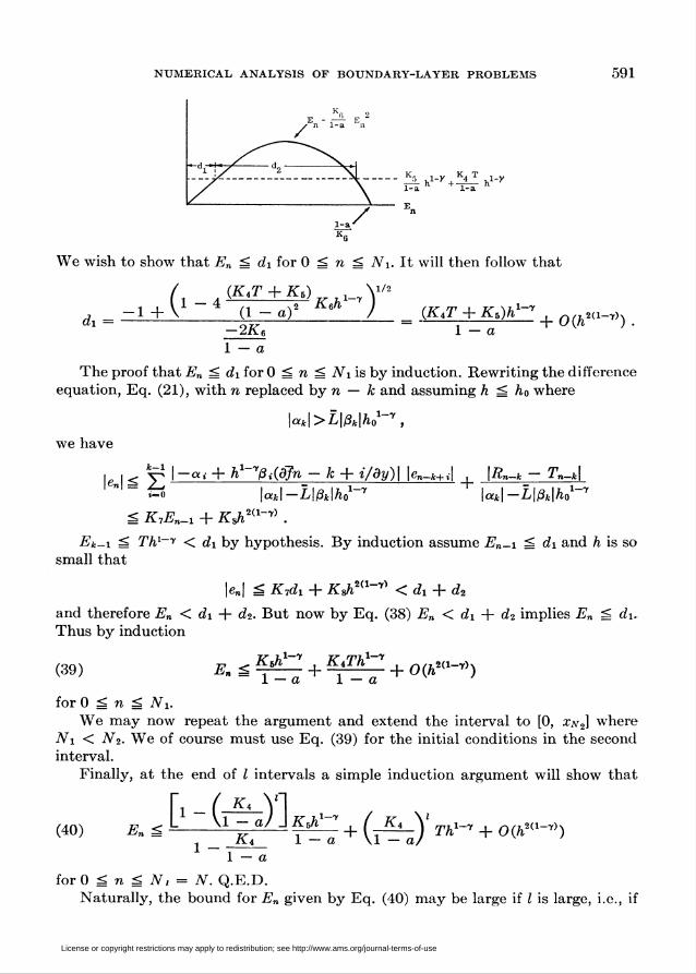
Geometrically, we have the following picture



i-y , 4 * ,i-y

We wish to show that En ^ di for 0 ^ n ^ Ax. It will then follow that

dx-1+0-

(A^r + a6)

(i - g)5

)l/2

= JKaT + K,)^-7 + 0(A2(1-,))-2A6

1 - a

1 - a

The proof that A„ á diforO ^ n g Ai is by induction. Rewriting the difference

equation, Eq. (21), with n replaced by n — k and assuming h ^ ho where

we have

kláE

|a*|>L|ftb|Äo 7,

ttf 4- h^ßjjdfn - fe + </ay)| k-*+.l , |7f„-fc - r„_*|

I^I-LIAIA,*-*5¡ K,En-x 4- 7Í3A2(1-7) .

+ak\-L\ßk\h0

l-T

Ek-x g TA1-1' < dx by hypothesis. By induction assume 7in_i ^ di and A is so

small that

k| á A7di + TCsA2"-1" < di + ds

and therefore 7£n < dx 4- (¿2. But now by Eq. (38) En < dx + 0*2 implies En è dx-

Thus by induction

(39) j-, ^, g5A KjTh . nn2(.i-v)\Ln - T=a~ + 1 - a + °{h >

forOln^ Ai.We may now repeat the argument and extend the interval to [0, xn2] where

Ai < A2. We of course must use Eq. (39) for the initial conditions in the second

interval.

Finally, at the end of I intervals a simple induction argument will show that

(40) E, s [' d''«)] aç + (_s_YKa, 1 — a \1 — a/

1 -A4

1 - a

T'A1"7 + 0(AA1-7')2(1-7) >

forO g n â A, = A. Q.E.D.Naturally, the bound for En given by Eq. (40) may be large if I is large, i.e., if


592 W. D. MURPHY

k-1 k

32'\Ci\ 31 m1=0 y=o

is much greater than 1. We therefore wish to minimize this sum. Since the roots

tjo ^ 1 on the unit circle do not yield p-stable difference schemes of higher pre-

cision than those roots inside the unit circle, we will exclude such roots for now.

A few important corollaries are :

Corollary 1. If the only essential root iroot on the unit circle) is tj0 — 1, and if

ak = 1 and ßj 2ï 0 for j = 0, 1, • • •, k, then the value of I in Theorem 2 inequality

(40)) is one.

Proof. Since ßj ^ 0 by consistency

p'(D = 32\ßA = (l-ri)(l -r2)---(l-r,_i),3=0

where pir¡) = 0, i = 1, 2, • • •, k — 1.

In Lemma 1 it was shown that

, , l/jak + 0(A1-7)) __1 + 0(A1-7).

' 0| - (fo - fi) (fo - ít) ■ ■ ■ (fo - f*-l) " p'(l)

Therefore, |C0| £y_0 \ßj\ ~ 1 ann ¿ can De chosen equal to 1. Q.E.D.

Corollary 2. If the only essential root is Yo = 1 and

(L-I)lColf .L + Oih1-7)^^31 <

where |f0| = 1 — Lhx"y 4- 0(A2(1~'1')), then the value of I in Theorem 2 is one.

Proof. The proof is obvious.

An example will illustrate how the value of I may be estimated in practice. Con-

sider the differential equation p?/ = —yiy — l)(20:c 4- 10) ; z/(0) = 2.

In the boundary layer for all 0 < A g A0, — 30 ^ fy ^ —10.

Example 2. Suppose Adam's method

A1+7F„+3 - Yn+2 = —- (97„+3 4- 197n+2 - 57„+1 4- Fn)

¿it

is used to calculate the solution to the above differential equation. Here

ICI g 1*1-jg.

Since fy is monotonie in the boundary layer

Li = L2 = Lx, L2 = Li = L2, etc. , ^ ¿rr = 0.8 ,30 24

where we have let a = 0.8 < 1,

,;Li = 30(0.435) = 13.1 , L2 = 30(0.435)' = 5.66 .

Outside of the boundary layer we make use of the following fact from the

asymptotic theory:



fyiyix, p), x) = /„(l, x) 4- 0(A7) = -20.T - 10 4- 0(A7)

for

- (2,iL)h7lnh7 giál.

Here/¡,(1, x) is independent of A and is monotonie ( — 30 =£ /»(l, #) = —10). Thus

we must increase Z by 2. Hence Z = 4. In practice it was observed that there was no

error build up outside of the boundary-layer region for p-stable schemes. Therefore,

the estimate I = 4 is to be considered an absolute maximum for the value of I in

this example.

Remark 1. The same proof of Theorem 2 could be used to obtain bounds for

p-stable methods instead of the less general relatively stable methods, but these

p-stable methods would require a much larger value of I.

Remark 2. Instead of considering — <x> < y < go we could have considered a

strip: 0 ^ x ^ 1 and \y — yix)\ < t where í is as large as is necessary in the proof.

Remark 3. If in Theorem 2 Rn and Tn are Oih^+w-^) and e< = Oih?«-^) for

i = 0, 1, ■ ■ ■, k — 1, then the same proof will lead to the result that en = Oihp(1~y))

for n = 0, 1, • • -, A.

5. Optimal Methods. By the "best method" or optimal method we will mean

the p-stable method which allows both I and Tn to be a minimum simultaneously.

By Corollary 1, I will have the value 1 if /3¿ ̂ 0, i = 0, 1, • • -, k and the only

essential root is f = 1. By using the methods outlined in Henrici [2] on optimal

methods we find that the "best methods" for the roots f = 1 and f = r where

\r\ < 1 take the form

Yn+2 - (1 -r-r)F„+i4-rFn

[(5 + r)Fn+2 + (8 - 8r)Fn+1 + (-5r - l)Fn] 4- TnA1"7

12

where

_ (1 + r) g,, 4J n — 24 "

Now if — 1 < r 5Í —1/5 all /3¿'s will be greater than or equal to zero. Therefore,

we merely pick r close to —1 in order to make Tn small.

For the case k = 3 let the roots be f = 1, rt, and r2 with |ri| < 1 and |r"2| < 1.

Of course if rx is complex then r2 must be its complex conjugate. The optimal

methods are characterized by:

ßi = (1/24) [9 + rx + r2 + rxr2] ,

ß2 = (1/24) [19 - 13 (n + r2) - 5rir2] ,

ßx = (l/24)[-5 - 13(ri 4- r2) + 19rxr2] ,

ßo = (1/24) [1 4- rx + r2 4- 9rir2] .

The condition that guarantees ßx è 0 is the most restrictive; we must require

Re rx ^ 0, Re r2 ^ 0 and -13(ri 4- r2) ^ 5 or 19rir2 ^ 5.


594 W. D. MURPHY

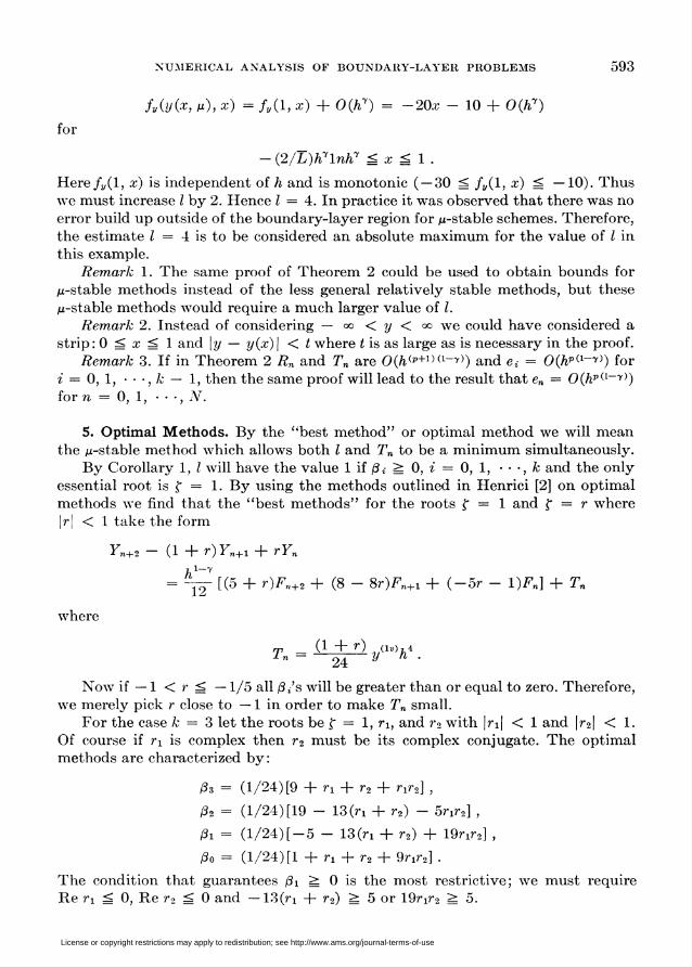
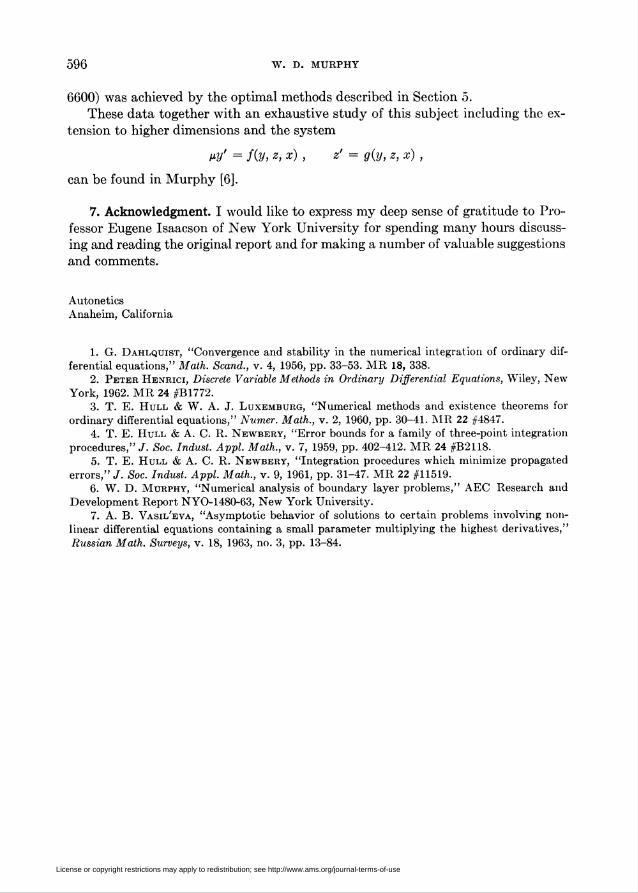
These inequalities will be satisfied if rx and r2 lie in the shaded region of Fig. 1

and are complex conjugates if either is complex. Note also that

Tn = (l/720)(-19 - llri - llr2 - 19nr2)

and has a minimum at rx = r2 — —11/19, which lies in the shaded region of Fig. 1.

Figure 1

For the case A; = 4 we choose the roots, 1, rx = —s,r2 = seie and r3 = se~ie,

0 < s < 1 and ic/2 ^ 8 ¿ ir, in order to simplify the arithmetic and to insure that

T„ = j^ [-27 - 27/w3 - 11 irx + r2 + n) -ll(nr2 4- nu 4- r2r3)]y(vlYx)h6

will be small. Note that the minimum occurs at s = 1.

The corresponding ß's for the optimal methods are given by :

ßi = 720 [251 + 19(ri + T2 + r3) + 11(rir2 + nu + r2Ti) + l9riT2r^ >

ßi = fh [646 ~ 346(ri + T2 + Tî) ~ 74(ri?-2 + rin + r2Ti) ~ 106rW>> ,

ß2 = ^ [-264 - 456{rx + r2 + n) + 456(r1?-2 4- nn 4- r2r3) 4- 264rir2r3] ,

^ = 72(3 [106 + 74(n + r2 + rs) + 346(rir2 + r^ + r*r«) - 646nr2r3] ,

ßo = 72^ [ — 19 — ll(ri + r2 + n) — 19(rir2 4- nn Y r2rz) — 251rir2r3l .

The analysis for the pYs is straightforward, and the conclusion is that we must

choose 0.695 ^ s < 1 and ir/2 ^ d ^ w to insure /3¿ ̂ 0, i = 0, 1, 2, 3, 4.

As k increases the analysis becomes much more difficult and even calculating

general expressions for the ß/s and Tn in terms of n, r2, • • -, rk-x is very tedious.

We therefore resort to a slightly different approach.

From our analysis of k = 2, 3, and 4 we suspect that for the r/s in the negative

half plane and near the unit circle there is some hope that for k > 4 all ß/s will

be greater than zero. We make use of the following formulas derived by Hull and

Newbery [5] for optimal methods :

fíiiik+2)hk+2 k fi

T»= n o.?m +Oihk+3), R=32*i-i xix-l)---ix-k)dx,{k 4- 1;! i=i J ¿-i

where



oci-x = aci 4- ai+x + • • • + ock

and

ß

k ri ,

V^ _ / *(•

1=1 J i—X

x — 1 ) • • • jx — k)d.c

(* - j)

for/ = 0, 1, • • -, k.

The above integrals can be calculated exactly by using the Newton-Cotes for-

mulas. We have programmed the CDC 6600 computer to calculate the values of ßj

for the limiting values of r\ where we suspect favorable results for the /3y's; that is,

for k even let one root be at f = 1, another at f = — 1, and all the remaining ones

at f = db i.For k odd let one root be at f = 1 and all others at f = úzi. We refer to this

choice of the roots at a-min. This is in contrast to a-max, where one root is chosen

at f = 1 and the remaining ones at f = —1.

Although both a-min and a-max define unstable schemes, in practice we would

choose one root at f = 1 and the other roots inside the unit circle but near the

roots of a-min or a-max when they lead to ß{ S: 0, i = 0, 1, • • -, fe.

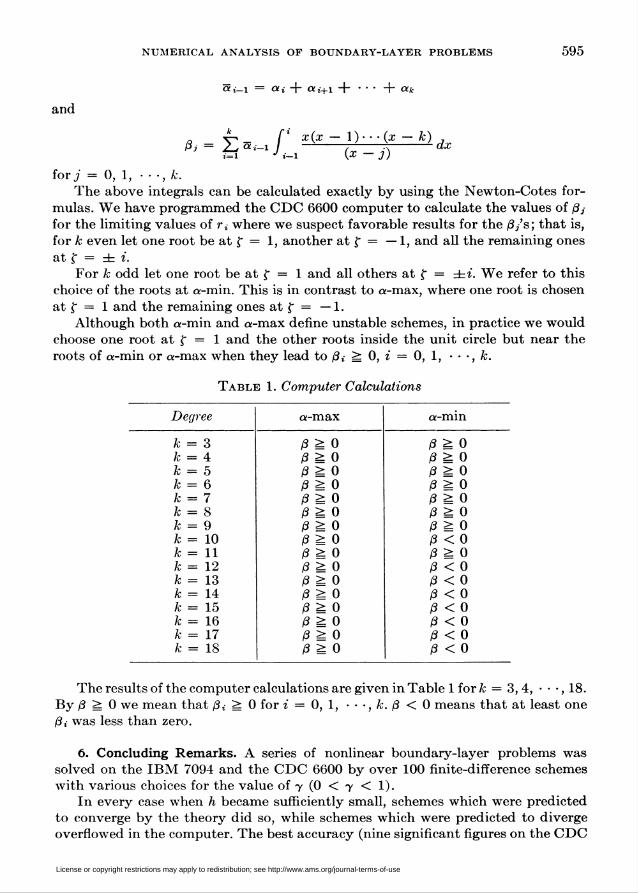
Table 1. Computer Calculations

The results of the computer calculations are given in Table 1 for fe = 3,4, • • •, 18.

By 0 2: 0 we mean that /3¿ 2: 0 for i = 0, 1, • • -, fe. ß < 0 means that at least one

ßi was less than zero.

6. Concluding Remarks. A series of nonlinear boundary-layer problems was

solved on the IBM 7094 and the CDC 6600 by over 100 finite-difference schemes

with various choices for the value of 7 (0 < 7 < 1).

In every case when A became sufficiently small, schemes which were predicted

to converge by the theory did so, while schemes which were predicted to diverge

overflowed in the computer. The best accuracy (nine significant figures on the CDC


596 W. D. MURPHY

6600) was achieved by the optimal methods described in Section 5.

These data together with an exhaustive study of this subject including the ex-

tension to higher dimensions and the system

fty' = fiv, 2, x) , z' = giy, z, x) ,

can be found in Murphy [6].

7. Acknowledgment. I would like to express my deep sense of gratitude to Pro-

fessor Eugene Isaacson of New York University for spending many hours discuss-

ing and reading the original report and for making a number of valuable suggestions

and comments.

Autonetics

Anaheim, California

1. G. Dahlquist, "Convergence and stability in the numerical integration of ordinary dif-

ferential equations," Math. Scand., v. 4, 1956, pp. 33-53. MR 18, 338.2. Peter Henkici, Discrete Variable Methods in Ordinary Differential Equations, Wiley, New

York, 1962. MR 24 #B1772.3. T. E. Hull & W. A. J. Luxemburg, "Numerical methods and existence theorems for

ordinary differential equations," Numer. Math., v. 2, 1960, pp. 30-41. MR 22 #4847.4. T. E. Hull & A. C. R. Newbery, "Error bounds for a family of three-point integration

procedures," J. Soc. Indust. Appl. Math., v. 7, 1959, pp. 402-412. MR 24 #B2118.5. T. E. Hull & A. C. R. Newbery, "Integration procedures which minimize propagated

errors," J. Soc. Indust. Appl. Math., v. 9, 1961, pp. 31-47. MR 22 #11519.6. W. D. Murphy, "Numerical analysis of boundary layer problems," AEC Research and

Development Report NYO-1480-63, New York University.

7. A. B. Vasil'eva, "Asymptotic behavior of solutions to certain problems involving non-

linear differential equations containing a small parameter multiplying the highest derivatives,"

Russian Math. Surveys, v. 18, 1963, no. 3, pp. 13-84.


numerical analysis of boundary-layer problems in … · numerical analysis of boundary-layer...

Documents