nuclear reactions for nuclear...
TRANSCRIPT

FACULTY OF SCIENCE
UNIVERSITY OF AARHUS
Nikolaj Thom
as Zinner: Nuclear R
eactions for Nuclear A
strophysicsD
issertation 2007
October 2007
Weak Interactions and Fission in StellarNucleosynthesis
Dissertation for the degreeof Doctor of Philosophy
Nikolaj Thomas ZinnerDepartment of Physics and Astronomy
Nuclear Reactions for Nuclear Astrophysics
Nuclear Reactions for NuclearAstrophysics
Weak Interactions and Fission in Stellar
Nucleosynthesis
Nikolaj Thomas Zinner
Department of Physics and AstronomyUniversity of Aarhus
Dissertation for the degree of Doctor ofPhilosophy
October 2007

@2007 Nikolaj Thomas Zinner2nd Edition, October 2007Department of Physics and AstronomyUniversity of AarhusNy Munkegade, Bld. 1520DK-8000 Aarhus CDenmarkPhone: +45 8942 1111Fax: +45 8612 0740Email: [email protected]
Cover Image: The evolution of the Universe from the Big Bang to the emer-gence of complex chemistry and Life.Printed by Reprocenter, Faculty of Science, University of Aarhus.

This dissertation has been submitted to the Faculty of Science at the univer-sity of Aarhus in Denmark, in partial fulfillment of the requirements for thePhD degree in physics. The work presented has been performed under thesupervision of Prof. Karlheinz Langanke. The work was mainly carried outat the Department of Physics and Astronomy in Aarhus. Numerous short-term visits to Gesellschaft fur Schwerionenforschung (GSI) in Darmstadt,Germany from 2005 to 2007 have been very fruitful toward the comple-tion of the thesis. The European Center for Theoretical Studies in NuclearPhysics and Related Areas (ECT*) in Trento, Italy is also acknowledged forits hospitality during the summer of 2004.
There is something fascinating about science.One gets such wholesale returns of conjecture
out of such a trifling investment of fact.Mark Twain (1835 - 1910)

Contents
Outline vii
Acknowledgements viii
List of Publications ix
1 Introduction 11.1 Children of the Stars . . . . . . . . . . . . . . . . . . . . . . . 11.2 Stellar Evolution and Supernovae . . . . . . . . . . . . . . . . 21.3 Physics of Core-collapse Supernovae . . . . . . . . . . . . . . 31.4 Nucleosynthesis . . . . . . . . . . . . . . . . . . . . . . . . . . 51.5 Angle of this Thesis Work . . . . . . . . . . . . . . . . . . . . 9
2 Theoretical Nuclear Models 102.1 Weak Interactions . . . . . . . . . . . . . . . . . . . . . . . . 10
2.1.1 Weak Interactions in Nuclei . . . . . . . . . . . . . . . 122.1.2 Cross Sections and Rates . . . . . . . . . . . . . . . . 15
2.2 Nuclear Structure Modeling . . . . . . . . . . . . . . . . . . . 192.2.1 Independent Particle Model . . . . . . . . . . . . . . . 212.2.2 Random Phase Approximation . . . . . . . . . . . . . 252.2.3 Reduction of Transition Operators . . . . . . . . . . . 372.2.4 Ground State and Model Space Considerations . . . . 412.2.5 Excitation Spectra Examples . . . . . . . . . . . . . . 422.2.6 Neutrino and Antineutrino Cross Section Comparison 44
2.3 Nuclear Decay Model . . . . . . . . . . . . . . . . . . . . . . . 462.3.1 Particle Decay Rates and Fission . . . . . . . . . . . . 472.3.2 Fission Fragments . . . . . . . . . . . . . . . . . . . . 502.3.3 The Dynamical Code ABLA . . . . . . . . . . . . . . 52
2.4 Unified Nuclear Model . . . . . . . . . . . . . . . . . . . . . . 532.4.1 Energy Mesh . . . . . . . . . . . . . . . . . . . . . . . 552.4.2 Monte Carlo and Statistics . . . . . . . . . . . . . . . 562.4.3 Neutrino Spectra and Folding . . . . . . . . . . . . . . 572.4.4 Anisotropy and Exotica . . . . . . . . . . . . . . . . . 60
iv

3 Muon Capture 633.1 Introduction . . . . . . . . . . . . . . . . . . . . . . . . . . . . 63
3.1.1 Previous Studies . . . . . . . . . . . . . . . . . . . . . 643.2 The Relativistic Muon . . . . . . . . . . . . . . . . . . . . . . 67
3.2.1 The Leptonic Current . . . . . . . . . . . . . . . . . . 683.2.2 The Non-Relativistic Limit . . . . . . . . . . . . . . . 723.2.3 The Relativistic Rate Formula . . . . . . . . . . . . . 74
3.3 Quenching of Multipoles . . . . . . . . . . . . . . . . . . . . . 873.4 The Residual Interaction . . . . . . . . . . . . . . . . . . . . . 883.5 Results and Discussion . . . . . . . . . . . . . . . . . . . . . . 893.6 Concluding Remarks . . . . . . . . . . . . . . . . . . . . . . . 92
4 Neutrinos and Proton-Rich Ejecta 954.1 Introduction . . . . . . . . . . . . . . . . . . . . . . . . . . . . 954.2 Neutrino Reactions on Matter . . . . . . . . . . . . . . . . . . 964.3 Hydrodynamical Simulation . . . . . . . . . . . . . . . . . . . 974.4 Network and Neutrinos . . . . . . . . . . . . . . . . . . . . . 994.5 νp-process Nucleosynthesis . . . . . . . . . . . . . . . . . . . 101
5 Neutrinos and the r-process 1075.1 r-process Nucleosynthesis . . . . . . . . . . . . . . . . . . . . 107
5.1.1 General Conditions . . . . . . . . . . . . . . . . . . . . 1075.1.2 The Neutrino-driven Wind . . . . . . . . . . . . . . . 108
5.2 UMP Stars and Neutrino-induced Fission . . . . . . . . . . . 1115.3 Neutrino-induced Fission on r-process Nuclei . . . . . . . . . 113
5.3.1 Initial Uranium Calculations . . . . . . . . . . . . . . 1145.3.2 r-process Nuclei . . . . . . . . . . . . . . . . . . . . . 1185.3.3 Preliminary Conclusions . . . . . . . . . . . . . . . . . 125
6 Fission and the r-process 1276.1 Introduction . . . . . . . . . . . . . . . . . . . . . . . . . . . . 1276.2 Nuclear Physics Input . . . . . . . . . . . . . . . . . . . . . . 127
6.2.1 β-delayed Fission . . . . . . . . . . . . . . . . . . . . . 1286.2.2 Neutron-induced and Spontaneous Fission . . . . . . . 1306.2.3 Fragment Distributions . . . . . . . . . . . . . . . . . 131
6.3 r-process Simulation Model . . . . . . . . . . . . . . . . . . . 1336.4 Results . . . . . . . . . . . . . . . . . . . . . . . . . . . . . . . 134
6.4.1 The Region and Role of Fission . . . . . . . . . . . . . 1346.4.2 The N = 184 Shell and Half lives . . . . . . . . . . . . 1386.4.3 The N = 82 Shell Closure . . . . . . . . . . . . . . . . 1396.4.4 Fission and Neutrinos . . . . . . . . . . . . . . . . . . 141
6.5 Nuclear Data Consistence . . . . . . . . . . . . . . . . . . . . 1426.6 Concluding Remarks . . . . . . . . . . . . . . . . . . . . . . . 143
v

7 Summary and Outlook 1457.1 Outlook - Nuclear Physics . . . . . . . . . . . . . . . . . . . . 1467.2 Outlook - Nuclear Astrophysics . . . . . . . . . . . . . . . . . 148
A Formalism and Conventions 150A.1 Units and Definitions . . . . . . . . . . . . . . . . . . . . . . . 150A.2 Angular Momentum Coupling and Spherical Functions . . . . 151A.3 Spherical Dirac Equation . . . . . . . . . . . . . . . . . . . . 154
B Neutrino Capture Rate Formula 155
C Nucleosynthesis and Entropy 157
Bibliography 159
vi
Outline
This thesis describes theoretical nuclear physics calculations for the pur-pose of expanding and improving the nuclear data input used in stellarnucleosynthesis modeling. In particular, the neutrino capture and β-decayweak interactions on a broad range of nuclei are considered. The decayof the daughter states resulting from the mentioned reactions are treatedin a statistical model. The latter includes both particle emission and fis-sion channels and provides fragments distributions for the fissioning nucleibased on a semi-empirical approach that agrees well with experimental data.These distributions have subsequently been implemented in simulations ofthe astrophysical r-process which is responsible for producing about halfthe heavy elements observed in nature. The neutrino capture processes onnuclei are also implemented in astrophysical modeling of ejected materialfrom exploding stars. Here it is found that an entirely new nucleosynthe-sis process operates. It requires the abundances of antineutrinos and canproduce many of the rare proton-rich elements whose origin is generallyconsidered unknown. The nuclear physics results presented in the thesis arefor reactions where very little experimental information is available. To en-sure that the theoretical model used is not at odds with existing knowledgewe have therefore also calculated total muon capture rates within the sameframework. The capture rates have been measured in many nuclei acrossthe nuclear chart and therefore provide a good benchmark to test the modelagainst.
In chapter one we give an introduction to the Supernova environmentwhich is the likely candidate site for the nucleosynthesis considered in laterchapters. Chapter two introduces and describes the nuclear structure andstatistical decay models that have been used in the calculations. Muon cap-ture on nuclei is described in chapter three, including novel correction termsfor relativistic effects that can influence the capture rate in heavy nuclei.Chapter four discusses the inclusion of neutrino and antineutrino reactionson nucleons and nuclei in nucleosynthesis calculations of early proton-richejecta from core-collapse Supernovae. In chapter five we discuss neutrinoreactions in the r-process with particular emphasis on the role of neutrino-induced fission and neutron emission. Chapter six presents and discussesresults from fully dynamical r-process simulations with all relevant fissionchannels and realistic fragment distributions included. Conclusions and out-look are given in chapter seven.
In the second edition (October 2007) misprints have been corrected andsome statements have been clarified.
vii

Acknowledgements
I would like to thank my adviser Karlheinz Langanke for proposing an inter-esting thesis project and for his continuous support and enthusiasm towardit. I am grateful to him for expanding my knowledge of physics, both fromthe academic point of view but surely also from a human perspective. Al-though most of his advise has proven invaluable there is one subject onwhich I strayed. Karlheinz once told me that I would never be able to finisha thesis without drinking coffee (as of this time I still do not drink it).
I wish to warmly thank Gabriel Martınez-Pinedo for his advise on nu-cleosynthesis issues discussed in this thesis and for providing the networkcalculations presented.
I wish to thank Carla Frohlich, Darko Mocelj, and F.-K. Thielemann inBasel for making our collaborations both pleasant and fruitful, and for takingcare of me during my visit in early 2004. I warmly thank Petr Vogel from theCalifornia Institute of Technology for suggestions and discussions on muoncapture and for a continued interest in its development. Furthermore, I owea debt of gratitude to Aleksandra Kelic and K.-H. Schmidt for providing uswith the ABLA code and for their help during its implementation. Thanksalso goes to Ivan Borzov for various discussion on nuclear structure details.
Thanks goes to Hans Fynbo for reading the draft version and correctinga host of trivial and non-trivial mistakes.
I wish to thank my friends and colleagues at the university in Aarhus forproviding a comfortable and interesting environment to work in. The bar onFriday was always fun. I also give many thanks to TAGEKAMMERET andFC Nordbyen 1993 for providing the needed break from studies whenevernecessary. I have many friends outside these places that have also beeninvaluable during the work, in particular Peter Busch Christiansen alwaysprovided comic relief and friendship in Vestervang for most of my life. Ihope he will continue to do so in the future.
Lastly I want to thank my family for putting up with my dreadful sched-ule and continuous canceling of various events during the past years. Youhave always provided comfort and support during the brief periods I haveactually been away from the university. Thanks to my mother, Inge Zinner,to whom my debt can never be repaid. Always remember that I am, andalways was, first and foremost Your son.
A special thanks goes to Anne Sevelsted. Her seemingly unending tol-erance for my less than perfect behavior and for my unrealistically involvedschedule over the years is not taken lightly. I have no way to describe howgrateful I am for your continued presence in my life.
viii

List of Publications[I] A. Kelic, N. T. Zinner, E. Kolbe, K. Langanke, and K.-H. Schmidt:
Cross Sections and Fragment Distributions from Neutrino-induced Fis-sion on r-Process Nuclei,Physics Letters B616 (2005) 48.
[II] C. Frohlich, P. Hauser, M. Liebendorfer, G. Martınez-Pinedo, E. Bravo,W. R. Hix, N.T. Zinner, and F.-K. Thielemann:The Innermost Ejecta of Core Collapse Supernovae,Nucl. Phys. A758, 27 (2005).
[III] C. Frohlich, P. Hauser, M. Liebendorfer, G. Martınez-Pinedo, F.-K.Thielemann, E. Bravo, N.T. Zinner, W.R. Hix, K. Langanke, A. Mez-zacappa, and K. Nomoto:Composition of the Innermost Core Collapse Supernova Ejecta,Astrophysical Journal 637 (2006) 415.
[IV] C. Frohlich, G. Martınez-Pinedo, M. Liebendorfer, F.-K. Thielemann,E. Bravo, W. R. Hix, K. Langanke, and N. T. Zinner:Neutrino-induced nucleosynthesis of A>64 nuclei: The νp-process,Phys. Rev. Lett. 96 (2006) 142502.Featured in: A New Way to Make Elements,Phys. Rev. Focus 17 (2006) story 14.
[V] N. T. Zinner, K. Langanke, and P. Vogel:Muon capture on nuclei: random phase approximation evaluation ver-sus data for Z=6-94 nuclei,Phys. Rev. C 74 (2006) 024326.
[VI] G. Martınez-Pinedo, A. Kelic, K. Langanke, K.-H. Schmidt, D. Mocelj,C. Frohlich, F.-K. Thielemann, I. Panov, T. Rauscher, M. Liebendorfer,N. T. Zinner, B. Pfeiffer, R. Buras, and H.-Th. Janka:Nucleosynthesis in neutrino heated matter: The νp-process and the r-process,Invited talk at NIC-IX, International Symposium on Nuclear Astro-physics - Nuclei in the Cosmos - IX, CERN, Geneva, Switzerland,25-30 June, 2006.Procedings contribution available through arXiv:astro-ph/0608490v1.
[VII] C. Frohlich, M. Liebendorfer, G. Martınez-Pinedo, F.-K. Thielemann,E. Bravo, N.T. Zinner, W.R. Hix, K. Langanke, A. Mezzacappa, andK. Nomoto:Composition of the Innermost Core Collapse Supernova Ejecta and theνp-process,AIP Conference Proceedings, Volume 847 (2006) 333.
ix

[VIII] C. Frohlich, W. R. Hix, G. Martınez-Pinedo, M. Liebendorfer, F.-K.Thielemann, E. Bravo, K. Langanke, and N. T. Zinner:Nucleosynthesis in Neutrino-Driven Supernovae,New Astronomy Reviews, Volume 50, Issue 7-8, p. 496 (2006).
[IX] C. Frohlich, M. Liebendorfer, F.-K. Thielemann, G. Martınez Pinedo,K. Langanke, N.T. Zinner, W.R. Hix, and E. Bravo:The Role of Neutrinos in Explosive Nucleosynthesis,Proceedings of the International Symposium on Nuclear Astrophysics- Nuclei in the Cosmos - IX. 25-30 June 2006, CERN., p.33.1.
[X] I.N. Borzov, K. Langanke, G. Martınez-Pinedo, A. Kelic, and N.T.Zinner:Neutrino-induced fission on nuclei,Proceedings of the International Symposium on Nuclear Astrophysics- Nuclei in the Cosmos - IX. 25-30 June 2006, CERN., p.78.1.
[XI] I. N. Borzov, J.J. Cuenca-Garcia, K. Langanke, G. Martınez-Pinedo,A. Kelic, and N.T. Zinner:Beta-decay of very neutron-rich nuclei near exotic shell-closures,EXON 2006 International Symposium on Exotic Nuclei,Khanty-Mansiysk, Russia, 17-22 July, 2006.
[XII] F.-K. Thielemann, C. Frohlich, R. Hirschi, M. Liebendorfera, I. Dill-mann, D. Mocelj, T. Rauscher, G. Martınez-Pinedo, K. Langanke, K.Farouqi, K.-L. Kratz, B. Pfeiffer, I. Panov, D.K. Nadyozhin, S. Blin-nikov, E. Bravo, W.R. Hix, P. Hoflich, and N.T. Zinner:Production of intermediate-mass and heavy nuclei,Prog. Part. Nucl. Phys. 59, 74 (2007).
[XIII] G. Martınez-Pinedo, D. Mocelj, N.T. Zinner, A. Kelic, K. Langanke,I. Panov, B. Pfeiffer, T. Rauscher, K.-H. Schmidt, and F.-K. Thiele-mann:The role of fission in the r-process,Prog. Part. Nucl. Phys. 59, 199 (2007).
[XIV] G. Martınez-Pinedo, D. Mocelj, N.T. Zinner et al.:The role of fission and the N = 82 shell closure in r-process nucle-osynthesis,to be submitted to Phys. Rev. Lett.
[XV] N.T. Zinner, A. Kelic et al.:Fission fragment distributions for r-process nucleosynthesis,in progress.
x
Chapter 1
Introduction
1.1 Children of the Stars
The beginning of the 21st century is a truly great time for science. Ideas,theories, measurements and observations are converging into what appearsto be a unified picture of the Universe we live in, Nature around us and evenour own existence. It is estimated that we have accumulated more scientificknowledge in the last 30-40 years than throughout the rest of our lifetimeon this planet. One of the greatest outcomes of this process is undoubtedlythat we can now explain the evolution of the universe from the time whenit was a mere 10−43 seconds old and all the way up to the emergency ofintelligent lifeforms. Although the answers obtained have brought alongeven more question and warrant continuing scientific efforts, we now havea remarkably insightful understanding of the laws of Nature. Our curiosityand thirst for knowledge has brought us a modern version of Genesis.
Our theories describe how the Big Bang started a Universe that wouldlater form clusters, galaxies and seemingly endless amounts of stars. Asthese stars evolve, they process the light elements hydrogen and helium intothe elements that we observe today. The very same elements that providethe conditions for life to develop. What this modern Genesis teaches us isthat we are all children of the stars. As such, one is not too surprised that thesynthesis of elements in stars is a hot topic. The basics are well understoodbut we still need to work on the accuracy of predictions. A mixture oflarge-scale hydrodynamical simulations, nuclear theories and experiments,knowledge of atomic transition lines, and an abundance of very accurateobservations are needed to achieve this goal.
In this thesis we will be concerned with the nuclear modeling aspects ofstellar nucleosynthesis. We wish to provide accurate nuclear physics inputfor simulations of element production. Before we embark on our journeyinto the details of the relevant nuclear physics, we will devote a few sectionsto explain basic features of the stellar environment that we consider.
1

CHAPTER 1. INTRODUCTION
1.2 Stellar Evolution and Supernovae
One of the greatest physicists of all time, the late Hans Bethe, pioneeredthe efforts to understand the reactions that power the stars in our night sky.He identified key fusion reactions that could produce the energy needed tobalance a stars gravitation and emit the light we observe. In particular, heproposed the so-called p-p reaction where protons from ionized hydrogenare converted into helium. This is the main source of energy in stars withmasses up to roughly that of our Sun. He also suggested what is known asthe CNO-cycle of Hydrogen burning, a process that had also been consideredearlier by Carl Friedrich von Weizsacker and which also operates in the Sunat the percent level.
The crucial thing for these burning processes to ignite at all is that theinitial cloud of gas that contracts to become a stellar object contains enoughmass. The gravitational contraction will heat the material, and if enoughmass is present the temperature will reach about 107 K needed for hydrogenburning to begin. This will happen when the protostar has mass in therange M = 0.1− 1.4M. Below this limit self-sustaining energy productionwill never be achieved and these objects become what is known as blackdwarfs or dead stars. In the cited mass range, the star will evolve similarlyto our Sun, burning hydrogen to helium for billions of years. As this is thelongest period among stellar evolution processes, it is no wonder that mostof the stars we observe are actually of mass close to M and in the hydrogenburning phase. These are known as main-sequence stars. When these starsfinally exhaust their hydrogen, they will expand and cool, and in the coreHelium burning starts. The light emitted will become more reddish and thestars are appropriately named Red Giants. They will presumably contractagain through a series of luminosity fluctuations and violent ejection of outermaterial. This will leave behind a so-called white dwarf, which will graduallycool and fade on a very long time scale of hundreds of billions of years,leaving again an inert black dwarf. When the mass is below about 1.4M,the so-called Chandrasekhar mass limit (we will return to this limit in thenext section), the star evolves essentially in the way described above. Thedetails of intermediate mass star M = 1.4−8M are rather involved. Theyreach the Helium burning phase and through various mass-loss mechanismthey eventually settle down in the white dwarf stage.
Stars of mass M ≥ 8M have much shorter lifetimes. The larger grav-itational energy released during contraction will lead to higher tempera-tures and this will make the burning of nuclear fuel faster. On top of that,these stars are capable of igniting the ashes of their previous burning stagesthrough continual contraction. As the energy output of each stage of burningdecreases compared to the previous stage, the star has to burn its fuel everfaster to balance gravity. This process of contraction and burning of ashescan continue up to the iron group, where the binding energy per nucleon has
2

CHAPTER 1. INTRODUCTION
a global maximum. The lifetime of a star is basically determined by the hy-drogen burning time as mentioned above. The more massive stars are denserand burn at higher temperatures so the Hydrogen is exhausted in less than10 million years. When the core reaches the iron group it cannot producemore energy and the inner parts of the star start to collapse. The star finallyexplodes in a cataclysmic event know as a core-collapse or Type II Super-nova. This will eject the matter above the inner core into the interstellarmedium and leave behind a neutron star. These are usually found observa-tionally in the form of so-called pulsars which emit radiation at extremelyprecise intervals. If the protostar is very massive (M & 20M), matter willaccrete on the neutron star in excess of the Chandrasekhar limit, making itcollapse into a Black Hole (recent work indicates that above around 60Mthere will again be heavy mass loss to prevent the star from becoming aBlack Hole).
1.3 Physics of Core-collapse Supernovae
Since we will be very concerned with the physical environment around a core-collapse Supernova, we will now describe the process in more detail. Whenthe iron-group is reached and nuclear burning seizes to produce energy,the core of the star starts to collapse as mentioned above. This process ishalted by the pressure of the degenerate electrons in the ionized material.Chandrasekhar showed that this can only stabilize a mass given by
MCh = 1.44(2Ye)2[1 + F (T )]M, (1.1)
where Ye is the electron fraction or number of electrons per baryon andF (T ) is a finite temperature correction which is usually 0.2−0.3 for massivestars. This is the Chandrasekhar mass limit. As the core contracts theFermi energy of the electrons increase, so electron capture on nuclei becomeenergetically favorable. This lowers Ye and thus also MCh. The capturesalso produce energetic electron neutrinos that escape the core. We thushave a reduction of energy and pressure and this will trigger almost free-fallcollapse in the core. 1 When densities are in excess of a few 1011 g/cm3, theneutrinos are scattered so frequently on nuclei that they cannot diffuse outof the core and become effectively trapped. The inner 0.7M now becomeequilibrated by electron-neutrino scatterings and collapses as a whole calledthe homologous core.
1Electron capture rates on protons are actually larger than the capture rate per nucleonon most nuclei. However, the collapse proceed at low entropy [1] and the temperature iskept low by neutrino losses, so most nucleons are bound in nuclei. It turns out that the lowentropy and high density enable β-decays to actually compete against electron capturesin the early stages of the collapse, so detailed studies have to take these into account also[2].
3

CHAPTER 1. INTRODUCTION
The collapse of the homologous core continues until nuclear densities of1014 g/cm3 are reached where the incompressibility of nuclear matter haltsthe implosion. This sudden stop creates a shock wave that moves outwardthrough the iron layers falling down from above. This will dissociate thematter and leave mostly free nucleons. One can make an estimate of theenergy of the shock and the mass it has to traverse. In doing so, one quicklyrealizes that the energy is insufficient to cause an explosion of the star. Mostlikely the shock simply stalls and becomes an accretion shock at a radiusof a few hundred kilometers. Matter will fall on it and be dissolved untilit runs out of energy. So it seems that another mechanism is needed forsuccessful explosions.
A likely candidate is the so-called delayed Supernova mechanism which isa way of reviving the shock by neutrinos. Electron captures on protons haveby now turned the remains of the homologous core into a protoneutron starthat attempts to cool as fast as possible. In doing so it emits huge amountsof neutrinos of all species. Furthermore there is a burst of neutrinos comingright when the shock moves through the core from electrons capturing on freeprotons. By neutrino absorption on free nucleons, energy can be transformedto the shock front, reviving it in less than a second by neutrino-nucleonreactions to produce a successful explosion.
To simulate this enormously complex stellar system is a great numericalproblem. One needs accurate modeling of magneto-hydrodynamics, shockpropagation, energy transport, lepton number tracking and neutrino dif-fusion. This naturally raises serious computational issues and consistentresults are often hard to come by. It now seems clear, however, that con-sistent explosions cannot be achieved in realistic spherical one-dimensionalmodels. Thus it would appear that we need multi-dimensional models whereconvection and rotational motion are handled properly. Studies where theseeffects are properly handled have been reported only very recently. Janka etal. have found consistent explosions in two-dimensional simulations throughthe neutrino-driven mechanism [3], whereas Burrows et al. now find explo-sions through acoustic oscillations (also in two dimensions) [4]. Both studieshave been carried out for several different progenitor masses and the resultsappear robust. They do, however, indicate that there could be more thanone mechanism that drives a Supernova explosion depending on the initialconditions. Models in three dimensions are underway and will likely teachus more about these newly discovered features.
As the solution of this problem could lie in accurate knowledge of thecharacteristics of this huge amount of neutrinos, people are also hoping fora galactic Supernova in the near future. By now, the detectors are ready forthe task of measuring the neutrino blueprint for all species, so that plenty ofthings could be learned if a Supernova exploded in our part of the Universe.
4

CHAPTER 1. INTRODUCTION
1.4 Nucleosynthesis
The origin of the chemical elements have long been a grand challenge forastrophysics. The lightest elements, H, He and some Li, were produced inthe early stage of the Big Bang. All other elements are produced in variouskinds of stellar processes. Nuclear burning for energy production will onlyproduce a limited range of species around the line of stability so the fact thatmany other elements are found in nature tells us that other mechanisms areoperating. Since the coulomb barrier will hinder fusion of heavy nuclei onehas to look for other means. The elemental abundance data of Suess andUrey [5] provided an answer since one could clearly see peaks at neutronnumbers 50, 82 and 126 (see figure (1.1)). This suggested that neutroncapture was responsible for heavy element synthesis and in two classicalpapers by Burbidge, Burbidge, Fowler, and Hoyle (B2FH) [6], and Cameron[7], the details of synthesis by neutron capture was described.
Figure 1.1: Breakdown of the solar system meteoritic neutron capture abundancesfor the s-process (red) and r-process (blue). Some prominent elements are notedat their approximate mass numbers. Adapted from [8].
Two main branches of heavy element production were identified: The
5
CHAPTER 1. INTRODUCTION
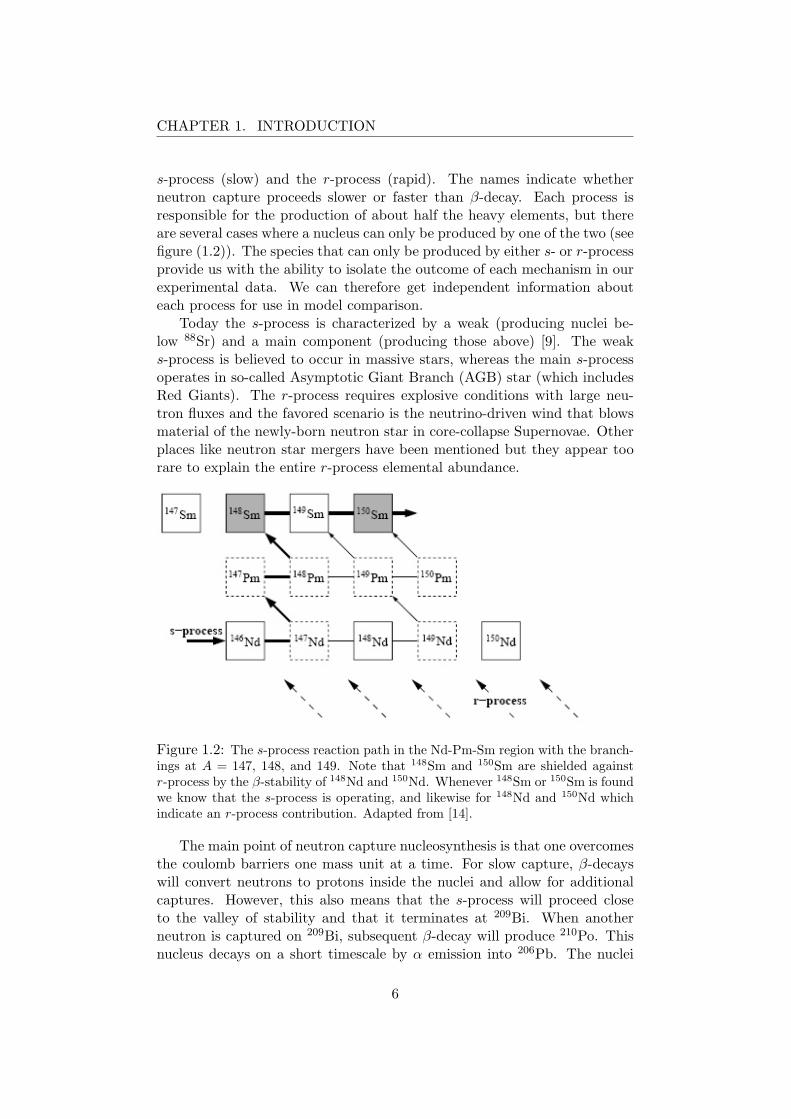
s-process (slow) and the r-process (rapid). The names indicate whetherneutron capture proceeds slower or faster than β-decay. Each process isresponsible for the production of about half the heavy elements, but thereare several cases where a nucleus can only be produced by one of the two (seefigure (1.2)). The species that can only be produced by either s- or r-processprovide us with the ability to isolate the outcome of each mechanism in ourexperimental data. We can therefore get independent information abouteach process for use in model comparison.
Today the s-process is characterized by a weak (producing nuclei be-low 88Sr) and a main component (producing those above) [9]. The weaks-process is believed to occur in massive stars, whereas the main s-processoperates in so-called Asymptotic Giant Branch (AGB) star (which includesRed Giants). The r-process requires explosive conditions with large neu-tron fluxes and the favored scenario is the neutrino-driven wind that blowsmaterial of the newly-born neutron star in core-collapse Supernovae. Otherplaces like neutron star mergers have been mentioned but they appear toorare to explain the entire r-process elemental abundance.
Figure 1.2: The s-process reaction path in the Nd-Pm-Sm region with the branch-ings at A = 147, 148, and 149. Note that 148Sm and 150Sm are shielded againstr-process by the β-stability of 148Nd and 150Nd. Whenever 148Sm or 150Sm is foundwe know that the s-process is operating, and likewise for 148Nd and 150Nd whichindicate an r-process contribution. Adapted from [14].
The main point of neutron capture nucleosynthesis is that one overcomesthe coulomb barriers one mass unit at a time. For slow capture, β-decayswill convert neutrons to protons inside the nuclei and allow for additionalcaptures. However, this also means that the s-process will proceed closeto the valley of stability and that it terminates at 209Bi. When anotherneutron is captured on 209Bi, subsequent β-decay will produce 210Po. Thisnucleus decays on a short timescale by α emission into 206Pb. The nuclei
6

CHAPTER 1. INTRODUCTION
heavier than bismuth found in Nature are therefore necessarily a result of ther-process. Here the neutron flux is very high and captures are faster than β-decay which means that one can produce very neutron-rich material (figure(1.3) illustrates the r-process path and the associated abundance peaks).When the flux drops below a certain critical value the r-process stops (thisis referred to as the freeze-out). The progenitor distribution of neutron-richnuclei will then decay back toward stability by β-decay. The produced peaksat neutron shells are slightly shifted compared to the s-process. The moreneutron-rich progenitors at freeze-out will have lower charges when theydecay back to stability (the left peaks in figure (1.1)). The r-process flowterminates when the nuclei get so heavy that fission becomes possible. Ifthe end-point is reached with sufficient neutron supplies remaining, one caneven have fission cycling where the fission fragments re-enter the captureprocess.
Figure 1.3: The figure shows a range of r-process paths. After decay to stabilitythe abundance of the r-process progenitors produce the observed solar r-processabundance distribution. The r-process paths run generally through neutron-richnuclei with experimentally unknown masses and half lives. Adapted from [15].
The mixing of material is another concern one has to consider with nu-cleosynthesis. The elements that are made in stars have to be ejected intothe interstellar medium in the right amount. Galactic chemical evolutionstudies give us information about how much material of a given compositionis needed to fit the final abundance pattern in our surroundings. Recent ob-servations of abundance patterns in ultra-metal poor stars have, however,suggested that the r-process yields are quite robust and very close to solar
7
CHAPTER 1. INTRODUCTION
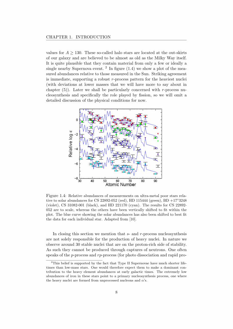
values for A ≥ 130. These so-called halo stars are located at the out-skirtsof our galaxy and are believed to be almost as old as the Milky Way itself.It is quite plausible that they contain material from only a few or ideally asingle nearby Supernova event. 2 In figure (1.4) we show a plot of the mea-sured abundances relative to those measured in the Sun. Striking agreementis immediate, supporting a robust r-process pattern for the heaviest nuclei(with deviations at lower masses that we will have more to say about inchapter (5)). Later we shall be particularly concerned with r-process nu-cleosynthesis and specifically the role played by fission, so we will omit adetailed discussion of the physical conditions for now.
Figure 1.4: Relative abundances of measurements on ultra-metal poor stars rela-tive to solar abundances for CS 22892-052 (red), HD 115444 (green), BD +173248(violet), CS 31082-001 (black), and HD 221170 (cyan). The results for CS 22892-052 are to scale, whereas the others have been vertically shifted to fit within theplot. The blue curve showing the solar abundances has also been shifted to best fitthe data for each individual star. Adapted from [10].
In closing this section we mention that s- and r-process nucleosynthesisare not solely responsible for the production of heavy nuclei. In nature weobserve around 30 stable nuclei that are on the proton-rich side of stability.As such they cannot be produced through captures of neutrons. One oftenspeaks of the p-process and rp-process (for photo dissociation and rapid pro-
2This belief is supported by the fact that Type II Supernovae have much shorter life-times than low-mass stars. One would therefore expect them to make a dominant con-tribution to the heavy element abundances at early galactic times. The extremely lowabundances of iron in these stars point to a primary nucleosynthesis process, one wherethe heavy nuclei are formed from unprocessed nucleons and α’s.
8

CHAPTER 1. INTRODUCTION
ton capture) mechanisms. The astrophysical site of these processes remainslargely unknown. Most suggestions assumes that they operate on seed nucleicoming from other kinds of nucleosynthesis. However, as we will discuss indetail later, we have recently found that proton-rich material can be pro-duced in all core-collapse Supernovae through a primary process (one wherethe seeds are produced at the same site). It is intimately connected withthe presence of neutrinos and has therefore been dubbed the νp-process [11].Other groups have confirmed these findings [12] using other Supernova mod-els, so the prediction seems robust. We have thus discovered a consistentway of producing proton-rich nuclei in generic Type II Supernova models.In addition, there are indications that the mechanism could also operate atother sites, such as gamma-ray bursts [13].
1.5 Angle of this Thesis Work
In this thesis we will attack the problems of stellar nucleosynthesis fromthe nuclear physics point of view. Weak interactions on nuclei are veryimportant here and the angle of this work is to improve and expand theknowledge about some of these reactions. For the simulation of the inner-most proton-rich ejecta in core-collapse Supernovae this involves calculationof neutrino and antineutrino captures on nuclei.
For r-process applications we will be concerned with weak reactions thatcan induce fission, such as neutrino captures and β-decays. This goal callsfor accurate models of nuclear structure and a good description of the sub-sequent decay of the excited nucleus through various fission and particleevaporation channels.
Parallel to this work, we have tested our nuclear structure model byusing it to calculate muon capture on nuclei. The weak interaction physicsis practically the same for this process and, contrary to neutrino captureand β-decay in neutron-rich nuclei, there are plenty of experimental dataavailable on muon capture. It is therefore a very nice way to check theconsistency and predictive power of the model.
9

Chapter 2
Theoretical Nuclear Models
2.1 Weak Interactions
The story of the weak force is a long and rich one. We will be rather briefin our discussion but refer the interested reader to the excellent accountof both history and formalism given in [17]. Shortly after Wolfgang Paulihad postulated the existence of the neutrino to account for hitherto unex-plained features in the energetics of β-decays, Enrico Fermi proposed thefirst theoretical description of the process [16]. He used an analogy fromelectromagnetic theory where the interaction hamiltonian has the so-calledcurrent-current form. Lorentz symmetry dictates that only certain terms areallowed and the general form of the interaction hamiltonian density becomes
Hint =GF√
2
∑i
Ci
(ψpOiψn)(ψeOiψν
)+ h.c., (2.1)
where ψn, ψp, ψe, ψν are the Dirac wave functions of the nucleons and leptonsparticipating in the β-decay, and GF is the famous Fermi coupling constant(1/√
2 is conventional). The Oi’s are operators that ensure that the currentshave the right transformation under the Lorentz group. These terms arescalar, pseudo scalar, tensor, vector, and axial vector respectively, or S, P,T, V, and A for short. The h.c. at the end stands for the addition ofthe hermitian conjugate term, so as to ensure that the total hamiltonianbecomes an hermitian operator. If we assume CPT conservation 1 one canshow that the constants Ci are real. It now took about twenty years beforereal progress was made again. In 1956 Lee and Yang made the ground-breaking observation that parity could be broken in weak decays [19]. Thefollowing year Wu et al. [20] confirmed this suggestion by examining β-decay
1This refers to the combined operation of charge conjugation (exchange particles forantiparticles), time reversal, and parity. In the construction of field theories this symmetryis almost always assumed. Note, however, that CP is actually violated in nature, so theassumption of CPT means that time reversal must be broken.
10
CHAPTER 2. THEORETICAL NUCLEAR MODELS
on 60Co. It become apparent that the weak interaction did not only violateparity but it did so in the maximal possible manner. For Dirac particles onecan define a left- and right-handed component, roughly according to whetherthe spin is along or opposite the direction of propagation. It turned outthat the weak force only couples to the left-handed component in β-decay.This was soon generalized by Feynmann and Gell-Mann, who proposed thatall weakly interacting particles should couple left-handedly [21]. This alsohas the consequence that only vector and axial vector terms are allowed inequation (2.1), so it actually makes the interaction a little simpler. This isknown as the V-A theory (vector minus axial vector). The next step wasthe advent of universality. This postulate states that the weak interactionis the same for all lepton families. Formally this amounts to the addition offurther leptonic current for muon and tau with the same couplings Ci. Thusa truly general picture had emerged.
It was, however, clear that the weak interaction had some totally differ-ent properties than electromagnetic forces. Being mediated by the masslessphoton, electromagnetic interactions have infinite range. This is not so forthe weak force, which is known to be extremely short ranged. A fact thatcould be understood if the carriers of the weak interaction are very mas-sive particles. But this is a real challenge since one could not really usethe lessons learned from the quantization of electrodynamics in the hugelysuccessful theory QED. In the quantum field theories used to describe ele-mentary phenomena there will always be infinities lurking. One can, how-ever, get rid of these when using so-called gauge theories. Unfortunatelythis requires all mediator particles to be massless, so a gauge theory of theweak interactions seemed doomed from the start. The sixties saw a decadeof intense investigation into this problem. This work finally succeeded withthe invention of the unified electroweak theory for which Glashow, Salamand Weinberg received the Nobel Prize in 1979. By applying the so-calledHiggs mechanism to a unified gauge theory of the weak and electromagneticforces, they found that some mediators can indeed be massive. The theoryalso predicted neutral weak currents that were later discovered at CERNin 1974. The question of infinities in this new class of gauge theories wassettled by t’Hooft in the early seventies. This earned him and his adviser,Martinus Veltman, the 1999 Nobel Prize.
Today the physics community has converged on the so-called StandardModel of particle physics. This includes the electroweak theory just de-scribed and a gauge theory of the strong interaction. 2 It has passed practi-cally all experimental tests so far with flying colors. However, recent yearshave seen several new developments in the areas of neutrino physics and cos-
2Some people like to include gravitation as a spin two gauge theory along with thestrong and electroweak parts. As the quantum theory of gravity still remains elusive weomit it here.
11
CHAPTER 2. THEORETICAL NUCLEAR MODELS
mology that overwhelmingly suggest that the Standard Model is inadequateand must be revised, expanded or replaced. Many in the physics commu-nity are also expecting to see evidence for supersymmetry when the nextgeneration of particle accelerators starts taking data, hopefully sometime inlate 2007. 3 The final word has surely not been said and we are facing someexciting decades ahead for fundamental physics.
2.1.1 Weak Interactions in Nuclei
Since our goals is to describe neutrinos and leptons interacting with nuclei,we need to address the question of nuclear currents. The hamiltonian givenin equation (2.1) contains a lepton and a nucleon current part. The leptonicpart was already described above by the V-A theory and we will leave itat that for the moment. Since nucleons also feel the effect of the stronginteraction, we cannot a priory expect it to have the same form. We have togo back to the principle of Lorentz invariance and work our way from there.The most general form that the nucleon current can have in momentumspace is
Jµi = u(p)[F1γ
µ +i
2MF2σ
µνqν + F3qµ
+ G1γµγ5 +
i
2MG2σ
µνqνγ5 +G3qµγ5]τiu(p′), (2.2)
where the nucleon is described by Dirac spinors u(p) and u(p′) with mo-mentum p and p′, M is the nucleon mass, and qµ = pµ − p′µ. The index ion the isospin operator τi is ±1 for the charge-changing interactions we areconcerned with. The constants in front of each term are called form factorsand must necessarily be Lorentz scalars. They can therefore only dependon q2 and are meant to describe the influence of the substructure of thenucleon on the weak processes in an effective way. We will now say a fewwords about how these are handled in our calculations.
The form factors F1 and G1 are the ones found in the leptonic V-A the-ory. However, here they are not merely ±1 since the nucleon has strongforces. F2 is a tensor-like term that is often called weak magnetism, refer-ring to its electromagnetic counterpart. The term G2 is called the inducedpseudo scalar coupling and is attributed to the fact that the strong nuclearforce is mediated by pions, which are pseudo scalar particles. The last two,F3 and G3, are known as induced scalar and tensor couplings. It is possi-ble to get some useful relations between the form factors by application ofsymmetry principles. Feynmann and Gell-mann did so by introducing theconserved vector current hypothesis [22]. An important consequence is thatthe form factors F1 and F2 can be taken directly from electron scattering.
3This paragraph was written in late 2006. At the time of revision of the manuscript,it seems more likely to be late 2008.
12

CHAPTER 2. THEORETICAL NUCLEAR MODELS
Furthermore since current conservation implies that the Fi terms must havevanishing divergence we have F3 = 0. At the same time Weinberg foundthat since the strong interaction is invariant under CPT and isospin therecan be no scalar or tensor terms in the current [23], leading to the conclusionG3 = 0 and once more F3 = 0. The pseudo scalar term G2 can actually berelated to the axial vector G1 by the famous Goldberger-Treiman relation[24]. It states that
G2(q2) =2MG1(q2 = 0)
q2 +m2π
(2.3)
where mπ is the pion mass. So we can get the pseudo scalar coupling fromthe axial vector one at zero momentum transfer.
As mentioned above, the form factors should take substructure into ac-count through their dependence on q2. We will always use what is knownas the dipole approximation for these functions [25]. This has the explicitform
Fi(q2) = Fi(q2 = 0)
1
1 +(
q2
m2
)2
, (2.4)
with a similar expression for the Gi’s. The mass m was taken to be m = 843MeV for vector parts and m = 1032 MeV for axial vector parts. Fromelectron scattering we get the vector couplings at q2 = 0; F1(0) = 1.00 andF2(0) = (µp − µn)/2M = 3.706/2M , where µp and µn are the magneticmoments of the proton and neutron respectively. The axial vector formfactor, G1, can be extracted from β-decay of the neutron, where a value ofG1(0) = 1.26 is found. However, as we shall discuss in more detail laterthere are renormalization effects in nuclear media to worry about. Thisphenomena is commonly referred to as in-medium quenching.
The weak processes that we would like to consider also require thatwe take the so-called Cabbibo mixing into account. In a 1963 paper [26],Cabbibo suggested that the hadron part of the weak current should be splitinto one that conserves strangeness (basically the number of strange quarksin a given reaction) and one that does not. In a more modern view involvingquarks this means that we simply have a current that can change down toup and one that changes down to strange (and vice versa). To maintainunitarity this split is given by a 2D rotation on the quark wave function, sothat the physical states are now
|d′〉 = cos θc|d〉+ sin θc|s〉 (2.5)|s′〉 = − sin θc|d〉+ cos θc|s〉, (2.6)
where θc is the Cabbibo angle. Experimentally it is found that sin θc ≈ 0.22and cos θc ≈ 0.98. We will be concerned exclusive with reactions that takeplace within the first family of quarks. This gives a cosine factor and we
13
CHAPTER 2. THEORETICAL NUCLEAR MODELS
will be using an effective Fermi coupling constant given by G = GF cos θc,where GF is the value obtained from muon decay (using universality).
In closing this section we address the assumptions we make when con-structing the nuclear current from the nuclear model that we introduce insection (2.2). We follow [18] and assume that the nuclear current can beexpressed in second quantization as a one-body operator at the origin. Thuswe have
Jµi (0) =
∑p′,s′,t′
∑p,s,t
〈p′, s′, t′|Jµi (0)|p, s, t〉a†p′,s′,t′ap,s,t, (2.7)
where the sums are over all allowed momenta, spin and isospin projections.Since we are using a one-body density we are effectively neglecting anymeson exchange currents, assuming that the many-body nuclear model wewill employ takes care of such contributions. The matrix elements are fromequation (2.2) and evaluated with free nucleon spinors. In reality the bindingof the nucleons will modify these spinors, but as it is much less than the restmass, we do not expect a big effect and we will neglect this. Through a seriesof reductions on the spinor expressions one can now make an expansion ofthe coordinate space currents in powers of the inverse nucleon mass [18].This results in the following terms
ρiV (~x) =
A∑j=1
GiE(j)τi(j)δ(3)(~x− ~xj) (2.8)
~J iV (~x) =
A∑j=1
GiE(j)
2Miτi(j)
[δ(3)(~x− ~xj)
−→∇j −
←−∇jδ
(3)(~x− ~xj)]
(2.9)
+−→∇ ∧
A∑j=1
GiM (j)2M
τi(j)~σ(j)δ(3)(~x− ~xj) (2.10)
ρiA(~x) =
GiA
2Mi
A∑j=1
τi(j)~σ ·[δ(3)(~x− ~xj)
−→∇j −
←−∇jδ
(3)(~x− ~xj)]
+−→∇ ·
A∑j=1
mµGiP (j)
2Mτi(j)~σ(j)δ(3)(~x− ~xj) (2.11)
~J iA(~x) =
A∑j=1
GiA(j)τi(j)~σ(j)δ(3)(~x− ~xj), (2.12)
where V is for vector current and A is for axial-vector current. Here we haveintroduced the Sachs form factors for the nucleon, GE(j) and GM (j) [27],which are different for protons and neutrons respectively. The axial vectorcoupling is denoted by GA and the pseudo scalar is called GP (evaluatedat the relevant momentum transfer through equation (2.4)). These are thecommonly used names and we will stick with them from now on. The index
14

CHAPTER 2. THEORETICAL NUCLEAR MODELS
i is again related to the isospin structure of the current and we maintain iton the couplings as they depend on isospin projection.
2.1.2 Cross Sections and Rates
We will now give basic formulas for the cross sections of neutrino and an-tineutrino scatterings and the rates for β-decays and charged lepton cap-tures. First we need to make a very important assumption about the Hilbertspace of nuclear states and that of the leptonic states. We assume that ournuclear model will always give us many-body states that have definite totalangular momentum and parity. Furthermore, we assume that the leptonicpart of the current-current interaction can be expanded in terms of functionsof well-defined angular momenta and parity. Now we can use partial waveanalysis and projection through the Wigner-Eckart theorem. This gives thefollowing expression for the matrix element of the interaction when summedand averaged over initial and final nuclear angular momentum projections[18]
12Ji+1
∑Mi
∑Mf
|〈f |Hint|i〉|2
=G2
24π
2Ji + 1[∞∑
J=0
(1 + ν · β) |〈Jf ||MJ ||Ji〉|2
+ [1− ν · β + 2(ν · q)(q · β)] |〈Jf ||LJ ||Ji〉|2
− 2[q · (ν + β)]Re〈Jf ||LJ ||Ji〉〈Jf ||MJ ||Ji〉∗
+∞∑
J=1
[1− (ν · q)(q · β)][|〈Jf ||J elJ ||Ji〉|2 + |〈Jf ||Jmag
J ||Ji〉|2]
− S 2[q · (ν − β)]Re〈Jf ||J elJ ||Ji〉〈Jf ||Jmag
J ||Ji〉∗], (2.13)
where all matrix elements are reduced by application of the Wigner-Eckarttheorem [28]. Ji is the total angular momentum projection of the initialnuclear state. For neutrino and antineutrino scattering ν is the unit vectorin the direction of the in-coming lepton and q is the unit vector in thedirection of the momentum transfer (q = k− ν), whereas β = |k|/ε is themomentum to energy ratio of the out-going electron or positron. For chargedlepton capture the roles are reversed giving q = ν − k, and for β-decay wehave both leptons in the final state so that q = ν + k. The factor S is +1for neutrino capture and β−-decay, and −1 for antineutrino capture and
15
CHAPTER 2. THEORETICAL NUCLEAR MODELS
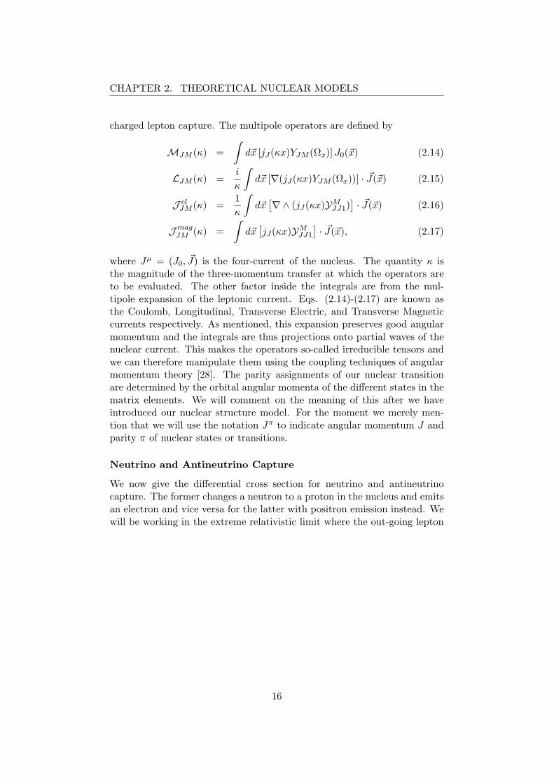
charged lepton capture. The multipole operators are defined by
MJM (κ) =∫d~x [jJ(κx)YJM (Ωx)]J0(~x) (2.14)
LJM (κ) =i
κ
∫d~x [∇(jJ(κx)YJM (Ωx))] · ~J(~x) (2.15)
J elJM (κ) =
1κ
∫d~x[∇∧ (jJ(κx)YM
JJ1)]· ~J(~x) (2.16)
JmagJM (κ) =
∫d~x[jJ(κx)YM
JJ1
]· ~J(~x), (2.17)
where Jµ = (J0, ~J) is the four-current of the nucleus. The quantity κ isthe magnitude of the three-momentum transfer at which the operators areto be evaluated. The other factor inside the integrals are from the mul-tipole expansion of the leptonic current. Eqs. (2.14)-(2.17) are known asthe Coulomb, Longitudinal, Transverse Electric, and Transverse Magneticcurrents respectively. As mentioned, this expansion preserves good angularmomentum and the integrals are thus projections onto partial waves of thenuclear current. This makes the operators so-called irreducible tensors andwe can therefore manipulate them using the coupling techniques of angularmomentum theory [28]. The parity assignments of our nuclear transitionare determined by the orbital angular momenta of the different states in thematrix elements. We will comment on the meaning of this after we haveintroduced our nuclear structure model. For the moment we merely men-tion that we will use the notation Jπ to indicate angular momentum J andparity π of nuclear states or transitions.
Neutrino and Antineutrino Capture
We now give the differential cross section for neutrino and antineutrinocapture. The former changes a neutron to a proton in the nucleus and emitsan electron and vice versa for the latter with positron emission instead. Wewill be working in the extreme relativistic limit where the out-going lepton
16

CHAPTER 2. THEORETICAL NUCLEAR MODELS
mass is neglected. In this case one finds(dσi→f
dΩl
)ν,ν
=G2ε2
2π2
4π cos2(Θ/2)2Ji + 1
F (Z ± 1, εf )
( ∞∑J=0
σJCL +
∞∑J=1
σJT
)
σJCL : =
∣∣∣〈Jf‖MJ(κ) +ω
κLJ(κ)‖Ji〉
∣∣∣2σJ
T : =(− q2
2κ2+ tan2(Θ/2)
)×[∣∣〈Jf‖Jmag
J (κ)‖Ji〉∣∣2 +
∣∣∣〈Jf‖J elJ (κ)‖Ji〉
∣∣∣2]∓ tan(Θ/2)
√−q2κ2
+ tan2(Θ/2)×[2<∣∣〈Jf‖Jmag
J (κ)‖Ji〉∣∣2 ∣∣∣〈Jf‖J el
J (κ)‖Ji〉∣∣∣2] , (2.18)
where the minus (plus) is for neutrino (antineutrino) respectively. Θ denotesthe angle between the leptons involved. The rest of the quantities are asin the previous section. The function F (Z ± 1, εf ) is the so-called Fermifunction, which is introduced to take the final-state interaction betweenlepton and daughter nucleus into account (see [29] and references therein).Since we will not be concerned with the direction of the out-going lepton, weshall always integrate the expression over all Θ to obtain the total capturecross section.
Muon Capture
The process of muon capture will be of great concern to us later as weuse it as benchmark for the nuclear structure model. This is the captureof a negative muon on a proton in the nucleus, resulting in its conversioninto a neutron and the emission of a muon neutrino. The nice feature ofthis process is the large rest mass of the muon: mµ = 105.6 MeV. Thisprovides a lot of energy to be shared between neutrino and nucleus. However,since the neutrino is (almost) massless it carries away most of the energy.Typical captures still leave 15-25 MeV of energy for nuclear excitation. Thismeans that the process can potentially excite giant resonance modes in thenucleus which are usually out of reach for β-decay and electron captures.Muon capture thus represents a valuable probe of these structures. Since thecapture turns a proton into a neutron we also have full or partial blockingof the so-called allowed transitions (such as the Fermi and Gamow-Teller) inmedium and heavy nuclei where neutrons always outnumber protons. Thismeans that the process has to go by higher-order transitions, also calledforbidden. We will say much more about these matters in chapter (3). Fornow we will merely give the capture rate formula usually employed in theliterature.
17

CHAPTER 2. THEORETICAL NUCLEAR MODELS
The most common experimental starting point for total muon capturerate measurements is a muon located in the atomic 1s orbit, so we will beassuming this at all times. In the non-relativistic limit this gives us a verysimple looking expression for the capture rate. We have
ωfi = G2ν2
2π
4π2Ji + 1
[∞∑
J=0
∣∣∣〈Jf‖M′J(ν)− L′
J(ν)‖Ji〉∣∣∣2
+∞∑
J=1
∣∣∣〈Jf‖J′magJ (ν)− J ′el
J (ν)‖Ji〉∣∣∣2]×R. (2.19)
Energy conservation gives us ν = mµ − εorbit + Enuci − Enuc
f , where εorbit isthe binding energy of the muon in the atomic 1s orbit. The operators arenow primed to indicate that they have the 1s muon wave function includedunder the integral. As the 1s is spherically symmetric, this does not altertheir tensor character. The factor R comes from the nuclear recoil and isgiven by
R =(
1 +ν
Mtarget
)−1
. (2.20)
Since we will always be interested in the total capture rate we have to sumthe above expression over all possible nuclear states of excitation energyE∗ = mµ − ν − εorbit. The nucleus has a number of states for each givenangular momentum J and parity. Naturally, we will truncate the sum at areasonable J where convergence is achieved.
The above formula apply when we can treat the muon as non-relativistic.This is a good approximation for nuclei of low charge. However, for highercharges corrections from relativistic effects can be expected. To see this,let us estimate the muon orbital energy in the 1s state by using the simplehydrogen-like formula. The usual ground state energy is about 13.6 eV. Thishas to be scaled by the muon-to-electron mass ratio and the charge squared.So we get 2.8 · Z2 keV. For a heavy nucleus like 208Pb with Z = 82 thisgives us 18.8 MeV, which is almost 20 percent of the muon rest mass. Thisestimate is actually a little too crude, since also the muon orbital radiuswill be smaller. It scales with inverse muon-to-electron mass ratio and withinverse charge, so it will be roughly 250 ·Z−1 fm. In 208Pb it is about 3 fm,so well inside the nucleus which has a radius of roughly 7.2 fm. The effectivecharge that the muon sees in its 1s orbit is therefore smaller than 82 and theenergy will thus be smaller than the estimate above. It is, however, clearthat the investigation of relativistic effects in muon capture is warrantedand this will be one of our main concerns in chapter (3).
β-Decay
The final weak process we will be concerned with is that of β-decay. As oneof our goals is to use these β-decay rates in r-process simulations, we will
18
CHAPTER 2. THEORETICAL NUCLEAR MODELS
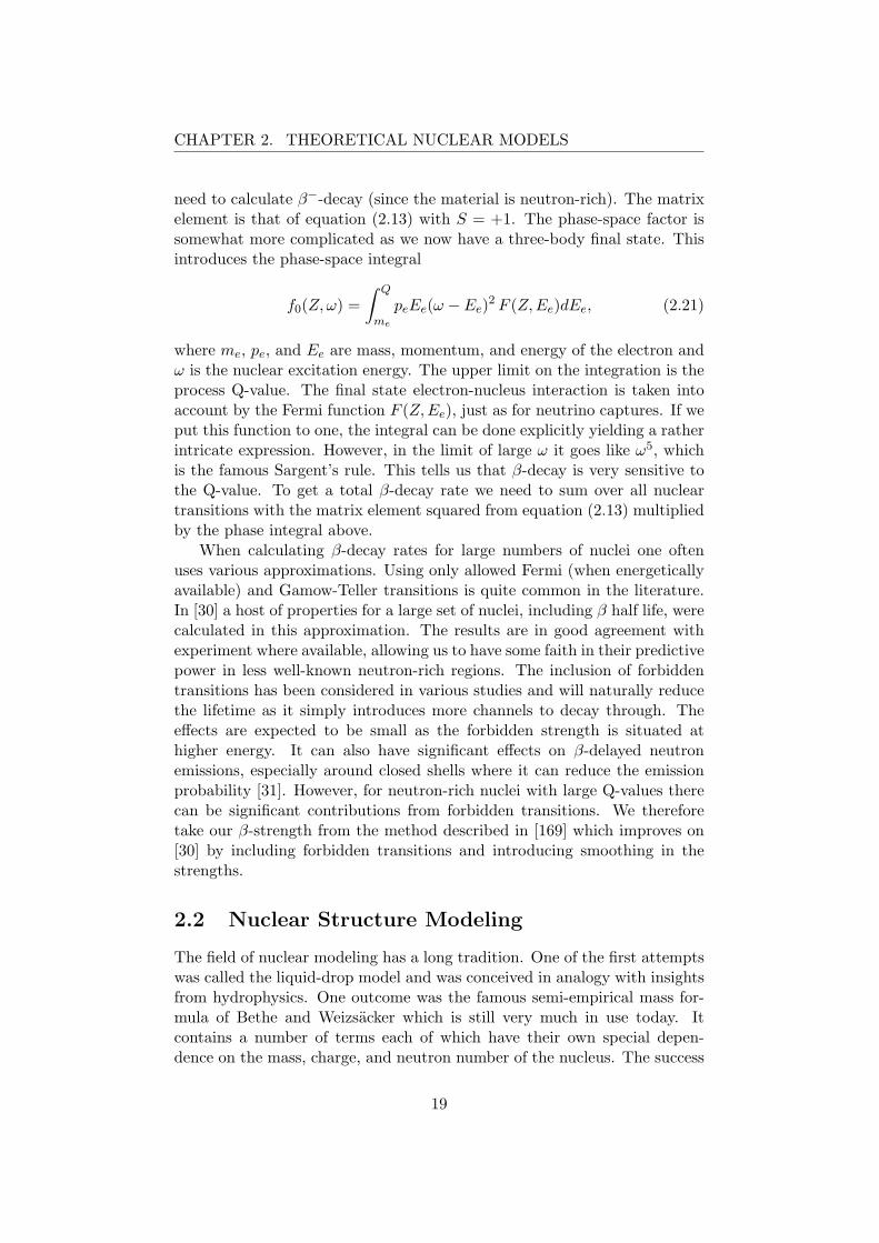
need to calculate β−-decay (since the material is neutron-rich). The matrixelement is that of equation (2.13) with S = +1. The phase-space factor issomewhat more complicated as we now have a three-body final state. Thisintroduces the phase-space integral
f0(Z, ω) =∫ Q
me
peEe(ω − Ee)2 F (Z,Ee)dEe, (2.21)
where me, pe, and Ee are mass, momentum, and energy of the electron andω is the nuclear excitation energy. The upper limit on the integration is theprocess Q-value. The final state electron-nucleus interaction is taken intoaccount by the Fermi function F (Z,Ee), just as for neutrino captures. If weput this function to one, the integral can be done explicitly yielding a ratherintricate expression. However, in the limit of large ω it goes like ω5, whichis the famous Sargent’s rule. This tells us that β-decay is very sensitive tothe Q-value. To get a total β-decay rate we need to sum over all nucleartransitions with the matrix element squared from equation (2.13) multipliedby the phase integral above.
When calculating β-decay rates for large numbers of nuclei one oftenuses various approximations. Using only allowed Fermi (when energeticallyavailable) and Gamow-Teller transitions is quite common in the literature.In [30] a host of properties for a large set of nuclei, including β half life, werecalculated in this approximation. The results are in good agreement withexperiment where available, allowing us to have some faith in their predictivepower in less well-known neutron-rich regions. The inclusion of forbiddentransitions has been considered in various studies and will naturally reducethe lifetime as it simply introduces more channels to decay through. Theeffects are expected to be small as the forbidden strength is situated athigher energy. It can also have significant effects on β-delayed neutronemissions, especially around closed shells where it can reduce the emissionprobability [31]. However, for neutron-rich nuclei with large Q-values therecan be significant contributions from forbidden transitions. We thereforetake our β-strength from the method described in [169] which improves on[30] by including forbidden transitions and introducing smoothing in thestrengths.
2.2 Nuclear Structure Modeling
The field of nuclear modeling has a long tradition. One of the first attemptswas called the liquid-drop model and was conceived in analogy with insightsfrom hydrophysics. One outcome was the famous semi-empirical mass for-mula of Bethe and Weizsacker which is still very much in use today. Itcontains a number of terms each of which have their own special depen-dence on the mass, charge, and neutron number of the nucleus. The success
19

CHAPTER 2. THEORETICAL NUCLEAR MODELS
of this average description of the nuclear masses means that we use it asguidance for much more advanced models to make sure that they get theseproperties right. Advanced versions of the model are actually still used instudies of fission since the complexity of the process makes the applicationof more microscopic models very difficult.
Naturally, the various forms of the liquid-drop model can only be helpfulin prediction of averaged properties of many-nucleon systems. A body ofexperimental evidence tells us that the individual nucleons act almost likeindependent particles. A single nucleon will feel the attraction from all theothers on average, but as soon as another one comes too close they willscatter away due to a hardcore interaction at small distances. Experimentshave shown that the mean free path is of order the size of the nucleus, soone does not expect the particles to come close very often. It is thereforereasonable to consider the nucleus as a system of particles that move aroundindividually in the average field of all the others. This is embodied in thehugely successful independent particle model (IPM) of the nucleus for whichGoeppert-Mayer and Jensen shared the 1963 Nobel Prize. Based on simplemean-field potentials analogous to those of atomic physics the model beauti-fully explains a host of properties. Perhaps most importantly it tells us whynuclei with certain numbers of protons or neutrons seem to exhibit strongerbinding than their neighbors in the nuclear chart. Simple, yet physically re-alistic, assumptions on the parameters of the potential reproduced perfectlythe so-called magic numbers of nucleons at the observed positions. A hugeleap forward had been taken.
The next natural goal for nuclear physicists was to try to explain the ap-pearance of such mean-field properties from basic knowledge of the nucleon-nucleon interaction. Atomic physicists had already considered this problemfor the pure coulomb potential using the Hartree-Fock method. Unfortu-nately this turned out to be less simple to apply in nuclei. The nucleon-nucleon potential is very complicated and early results were not promising.Today we have a number of refined methods that give us much better agree-ment. No-core Shell Model, Green’s function Monte Carlo, and hyperspheri-cal expansion of the N-body Schrodinger equation are a few of the successfulmodern techniques used. However, some of these are extremely computa-tionally intensive and only light or medium nuclei have been studied. Sothere is still plenty of work to be done in improving these methods.
The models mentioned above are typically used for prediction of ground-state properties. In applications where nuclear reactions are considered wealso need to have an accurate description of the nuclear excitation spec-tra. This requires a model that can handle both single-particle excitationsand also the very important coherent nuclear states where many particlesconspire to create broad structures in the spectrum at higher energies thatcannot be described by an IPM. The latter are often referred to as giantresonances. The nuclear structure model method of choice is a Large-Scale
20
CHAPTER 2. THEORETICAL NUCLEAR MODELS
shell model. The approach is to start from an IPM with a given number ofnucleons and then diagonalize some residual interaction in a basis consistingof all possible arrangements of the particles in the IPM potential. With two-or even three-body interactions the number of configurations grows very fast,so the matrices are huge, restricting the method to light or medium systems.However, techniques using effective interactions and truncated model spaceswith inert cores of non-interacting nucleons are becoming more advanced.With computers also gaining power, the future for large-scale modeling looksbright.
The goal of the work described in this thesis is to calculate weak interac-tions on a great number of nuclei, so shell model calculations are ruled outby memory constraints even in todays supercomputers. We need insteada fast method that can reproduce the giant resonances in the spectra asthey turn out to be particularly important for our purposes. We thereforeuse the random phase approximation (RPA). This method starts from anIPM and then diagonalizes a residual interaction in a basis consisting of allconfigurations obtained by moving just one particle at a time. The basis isrestricted to one particle-one hole excitations and is therefore much smallerthan that used in large-scale shell model. This makes the method very fastfor applications where particle-hole structures are sufficient.
Once we have our nuclear structure model that give us an excitationspectrum and probabilities to populate each state, we would like to considersubsequent decay of the excited daughter nucleus. This will be done underthe assumption of the formation of a compound nucleus, a picture of nucleardecay first advocated by Niels Bohr in the late 1930ties. It assumes that thedecay of the excited state is slow compared to the time it takes the nucleus todistribute the excitation energy among all the degrees of freedom that havequantum numbers satisfying all conservation laws. When this is achieved,the state of the nucleus is given by a statistical distribution, independentof the way the excited state was formed. Under these assumptions one canemploy statistical decay models that use the nuclear density of states tofind the widths of relevant decay channels. This naturally requires detailedknowledge of nuclear statistical properties over a wide range of energies socare must be taken that choices of masses, shell effects, pairing etc. areconsistent. This will be discussed later when we introduce the statisticaldecay models that we have used.
2.2.1 Independent Particle Model
The first step in our nuclear structure modeling is to set up a reliable inde-pendent particle model to provide us with realistic single-particle energiesand wave functions. As our goal is to calculate interactions for a range ofnuclei that covers basically the whole nuclear chart, we need something uni-versal with only a small amount of parameters needing adjustment for each
21
CHAPTER 2. THEORETICAL NUCLEAR MODELS
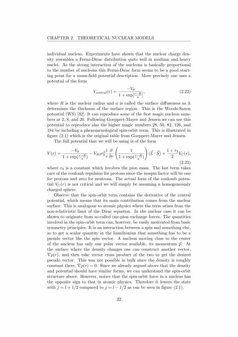
individual nucleus. Experiments have shown that the nuclear charge den-sity resembles a Fermi-Dirac distribution quite well in medium and heavynuclei. As the strong interaction of the nucleons is basically proportionalto the number of nucleons this Fermi-Dirac form seems to be a good start-ing point for a mean-field potential description. More precisely one uses apotential of the form
Vcentral(r) =−V0
1 + exp[ r−Ra ]
, (2.22)
where R is the nuclear radius and a is called the surface diffuseness as itdetermines the thickness of the surface region. This is the Woods-Saxonpotential (WS) [32]. It can reproduce some of the first magic nucleon num-bers at 2, 8, and 20. Following Goeppert-Mayer and Jensen we can use thispotential to reproduce also the higher magic numbers 28, 50, 82, 126, and184 by including a phenomenological spin-orbit term. This is illustrated infigure (2.1) which is the original table from Goeppert-Mayer and Jensen.
The full potential that we will be using is of the form
V (r) =−V0
1 + exp( r−Ra )− VSOr
20
1r
∂
∂r
(1
1 + exp( r−Ra )
)(~L · ~S) +
1 + τ32
VC(r),
(2.23)where r0 is a constant which involves the pion mass. The last term takescare of the coulomb repulsion for protons since the isospin factor will be onefor protons and zero for neutrons. The actual form of the coulomb poten-tial VC(r) is not critical and we will simply be assuming a homogeneouslycharged sphere.
Observe that the spin-orbit term contains the derivative of the centralpotential, which means that its main contribution comes from the nuclearsurface. This is analogous to atomic physics where the term arises from thenon-relativistic limit of the Dirac equation. In the nuclear case it can beshown to originate from so-called one-pion exchange forces. The quantitiesinvolved in the spin-orbit term can, however, be easily motivated from basicsymmetry principles. It is an interaction between a spin and something else,so to get a scalar quantity in the hamiltonian that something has to be apseudo vector like the spin vector. A nucleon moving close to the centerof the nucleus has only one polar vector available, its momentum ~p. Atthe surface where the density changes one can construct another vector,∇ρ(r), and then take vector cross product of the two to get the desiredpseudo vector. This was not possible in bulk since the density is roughlyconstant there; ∇ρ(r) = 0. Since we already argued above that the densityand potential should have similar forms, we can understand the spin-orbitstructure above. However, notice that the spin-orbit force in a nucleus hasthe opposite sign to that in atomic physics. Therefore it lowers the statewith j = l + 1/2 compared to j = l − 1/2 as can be seen in figure (2.1).
22

CHAPTER 2. THEORETICAL NUCLEAR MODELS
Figure 2.1: The independent particle model illustration table from the classicaltext of Goeppert Mayer and Jensen. Notice the assigned numbers on the far left.These are the harmonic oscillator shell numbers of the nuclear orbits.
23

CHAPTER 2. THEORETICAL NUCLEAR MODELS
We now go through the choice of parameters for the potential in eq.(2.23). For the nuclear radius we use the standard formula R = r0 · A1/3.We have worked with r0 = 1.22 fm, which is close to the value given in[32] and [33]. For protons the Coulomb potential should in principle use thecharge radius instead. In [33] it was found that results based on the WSpotential are not very sensitive to this parameter and we will simply use thenuclear radius in this term as well. There is another radius to be specifiedin the WS term that multiplies the spin-orbit operator. Again we havesimply taken the nuclear radius as we have found our results to be insensitiveto this parameter. For the diffuseness we use a value slightly below therecommendation of [33], working with a = 0.53 fm in all calculations. Thisvalue is probably better for lighter nuclei where the harmonic oscillator orsquare well potentials are good approximations. However, previous studiesinto isotope effects in total muon capture rates have shown that it requireslarge changes in a for any effects to be seen [34]. In that paper, a = 1.00fm was used to obtain noticeable differences in the rates on very neutron-rich Sn isotopes compared to the muon capture rates with our standardvalue of a = 0.53. Based on this observation we have simply kept a = 0.53fm in both central and spin-orbit terms. The magnitude of the spin-orbitinteraction VSO was set to 17.9 MeV in all calculations. This value was foundby considering experimental numbers on medium mass nuclei. It agrees wellwith the value given in [33]. However, there are data suggesting that VSO
depends slightly on the asymmetry parameter (N − Z)/A. We have testedthis in the case of muon capture and found that changes of a few MeV makelittle difference, presumably because the dependencies are taken care of bythe derivative of the central potential. We therefore keep the same constantVSO.
The numerical technique used to obtain the WS eigenvalues and eigen-functions is truncation and diagonalization. The starting point is a basis con-sisting of the well-known eigenfunctions of the three-dimensional isotropicharmonic oscillator. We have used up to ten major shells to achieve goodconvergence. Notice that the coulomb part means that neutrons and pro-tons have different potentials so we solve for these independently. A possibledrawback of this method comes from the fact that all these functions arebound states from the beginning, and the solution for the WS potential willthus also always have exponential tails and all eigenvalues will be discrete.We will still get positive energy eigenvalues, but the corresponding eigen-functions do not have the correct physical boundary conditions. Deep in thepotential we expect the results to be quite accurate but for loosely boundstates it is questionable. However, as we will see when we discuss muon cap-ture in chapter (3) our simple model with only these discrete states worksvery well [35].
A final parameter that our model needs from the outside is somethingto fix the single-particle Fermi level. We need to have a good idea about the
24

CHAPTER 2. THEORETICAL NUCLEAR MODELS
energy of the orbit where the last proton and neutron is located. The energyof these levels depends on whether the process changes neutron to protonor vice versa. For muon and antineutrino capture the charge is decreasedby one, so we change a proton in the mother nucleus into a neutron in thedaughter. This means that proton orbits belong to the mother and neutronorbits belong to the daughter. A good approximation for the energy of thelast proton level is therefore the proton separation energy Sp in the mothernucleus (A,Z) and for the neutron level it is the neutron separation energySn in the daughter (A,Z − 1). The processes of neutrino capture and β-decay convert neutron to proton. We will thus fix the neutron orbits by Sn
in the mother (A,Z) and the proton orbits by Sp in the daughter (A,Z+1).Sn and Sp were calculated based on the mass table of Moller, Nix, and Kratz[30].
2.2.2 Random Phase Approximation
To handle the nuclear excitation response we will use the random phaseapproximation. This is a well-established and computationally fast method.The basic idea is to try to obtain excited states of the nucleus by expandingthese on a very simple basis of IPM wave functions. The basis consists ofthe so-called particle-hole states, which are IPM states where we allow themovement of one particle to some unoccupied orbit, leaving behind a holein one of the lower orbits. The principles are thus very much in tune withthe single-particle picture. However, the new element is the introductionof a residual interaction which acts between the particles around the Fermilevel. We can diagonalize this interaction in the particle-hole basis and thenhopefully get an accurate description of the excited states. This strategyis called the Tamm-Dancoff approximation (TDA) or simple particle-holetheory [36]. TDA has the problem that it does not satisfy important sumrules, which causes it to underestimate low-lying collective excitations [36].What we can do better in this situation, is to take into account the effectof the residual interaction on the ground state itself, so that it is not sim-ply the naive IPM state, but rather a superposition of particle-hole states(like the excited states in the TDA method). This procedure is called therandom phase approximation (RPA). Originally it was introduced by Bohmand Pines [37] to describe plasma oscillations in electron gases. The termRPA referred to the neglect of modes with frequencies different from thecollective field on the assumption that they would have arbitrary phasesand thus cancel out on average. As we will see when we discuss the RPAequations below, the phases that are assumed to cancel in nuclear applica-tions are those of fermion exchange correlations, allowing one to treat thecorresponding operators as bosons. This also warrants the alternative namequasi-boson approximation.
We will always be working with discrete energy states (due to the bound
25
CHAPTER 2. THEORETICAL NUCLEAR MODELS
nature of the IPM states as introduced earlier). This is often called the sim-ple RPA (SRPA). For loosely bound systems one should ideally include alsocontinuum states in the equations, leading to the continuum RPA (CRPA).However, as was shown in [35], there is little difference between the twomethods when calculating total muon capture rates for a broad range ofnuclei. We therefore work strictly with the simpler SRPA model.
Basic RPA Equations
We start by looking at the TDA equations as a warm-up exercise. Firstwe define creation operators for the TDA states, which are the followingsuperpositions of particle-hole states
Q†TDA,ν =∑m,i
Xνm,ia
†mai, (2.24)
where m labels unoccupied states and i labels occupied states. ν keeps trackof the TDA solutions. The TDA vacuum is defined by the equation
QTDA,ν |0〉TDA = 0 (2.25)
for all ν. Now we approximate the TDA vacuum by the IPM ground state,and using the so-called equations-of-motion method [36, 32] 4, we get thefollowing eigenvalue equation for the TDA solutions∑
n,j
(εm,iδmnδij + vmjinXνn,j = Eν
TDAXνm,i, (2.26)
where εm,i is the difference of particle and hole orbital energies, m,n re-fer to occupied, and i, j to unoccupied states. The residual particle-holeinteraction is given by the following matrix element of IPM wave functions
vmjin = 〈mj|v|in〉 − 〈mj|v|ni〉 (2.27)
which has a direct and an exchange part.The RPA equations are produced by generalizing the operators for the
TDA states above to also include terms that annihilate particle-hole pairs.The creation operators for the RPA states then take the general form
Q†RPA,ν =∑m,i
Xνm,ia
†mai −
∑m,i
Y νm,ia
†iam (2.28)
4The method is inspired by the harmonic oscillator where the hamiltonian can bewritten as a product of annihilation and creation operators. Making such an ansatz forthe nuclear hamiltonian and the using a variation of the operators Qν will give the TDAand RPA equations [36, 32].
26

CHAPTER 2. THEORETICAL NUCLEAR MODELS
with the same meaning of indices as above and a conventional minus signbetween the two terms. Again we define the vacuum by
QRPA,ν |0〉RPA = 0 (2.29)
for all ν. Going through exactly the same steps as for the TDA now gives usthe RPA eigenvalue equations. Since there are now two sets of coefficients,X and Y , to be determined, the equations are most conveniently displayedin matrix form(
A BB∗ A∗
)(Xν
Y ν
)= ~Eν
RPA
(1 00 −1
)(Xν
Y ν
), (2.30)
where the dimension is twice the number of possible particle-hole pairs inthe model space of IPM states. The matrix A is the same as for the TDAstates
Aminj = εm,iδmnδij + vmjin, (2.31)
whereas that for B isBminj = vmnij . (2.32)
The name quasi-boson approximation originates from the use of the IPMground state instead of the RPA vacuum. When we take the commutator ofdifferent particle-hole pairs and make the replacement of the ground statewe get
RPA〈0|[a†iam, a†naj ]|0〉RPA ≈IPM 〈0|[a†iam, a
†naj ]|0〉IPM = δmmδij . (2.33)
We recognize that the approximation effectively means treating the particle-hole pair operators as bosons. This naturally violates the Pauli principleand this is where we need the contributions from the neglected fermioniccommutator terms to be small or cancel due to random phases.
The real ground state of the many-body system can be built from theIPM with the addition of all nparticle-nhole states by completeness. Thenew feature of the RPA over the TDA is that it also allows one to annihilateparticle-hole pairs, so it includes correlations in the ground state. When welook at the equations we see that the TDA approximation is recovered if weset Y ν
m,i = 0. These coefficients are therefore a measure of the ground statecorrelations.
For the RPA to be a good approximation we need two conditions onthe coefficients X and Y . The solutions should have many Xν
m,i of the sameorder of magnitude, that is they should have a very collective character. Thismeans that each particle-hole pair has a small probability of being excitedand therefore the violation of the Pauli principle for individual pairs is notimportant. In addition, the Y ν
m,i are also required to be small in magnitude,since otherwise the IPM ground state would be too far from the RPA ground
27
CHAPTER 2. THEORETICAL NUCLEAR MODELS
state and our approximation would break down. This can happen and isoften referred to as the collapse of the ground state.
As mentioned above we treat protons and neutrons independently inthe IPM. This means that we must also do so in the RPA equations. Asdescribed in the IPM section, the charge-changing processes of interest willchange protons to neutrons and vice versa. We incorporate this into the RPAdescription by taking the particle-hole pairs so that they reflect the isospindirection of the process. If we are concerned with a process that changesneutron to proton then all particle states are neutrons and all hole statesare protons and vice versa. We are thus working in a basis that consists ofmixed particle species.
What we are ultimately interested in with our nuclear structure modelis to be able to calculate transition matrix elements. For our purposes theyare one-body operators between the ground state of the mother nucleus andexcited states in the daughter. If we have an hermitian one-body transi-tion operator T, then the RPA gives the following simple expression for thematrix element
RPA〈0|T |ν〉RPA =∑m,i
Tm,iXνm,i + Tm,iY
νm,i, (2.34)
where Tm,i = 〈m|T |i〉 is the matrix element of the operator with the relevantIPM states. Whereas the wave functions for the excited states are notvery accurate, the RPA is known to do well in describing such transitionelements. 5 This is because such transitions elements depend not on theabsolute wave functions but on their internal relationships. This is exactlythe philosophy behind the equations-of-motion method that was used toderive the RPA equations above [36].
We have previously mentioned that we are interested in nuclear statesof good total angular momentum. To achieve this in the RPA equations wehave to switch to the coupled representation where the creation operatorsfor particle-hole excitations carry good angular quantum numbers. Theanalogue of equation (2.28) in the coupled case is
Q†RPA,ν(JM) =∑m,i
Xνm,iA
†m,i(JM)−
∑m,i
Y νm,i (−1)jm+ji+M Am.i(JM).
(2.35)The new creation and annihilation operators are constructed by using stan-
5This is in close analogy with standard perturbation theory where the energy correc-tions in lowest order are often very good and the wave functions are notoriously bad. TheRPA can actually also be derived as the small amplitude limit of time-dependent Hartree-Fock theory (TDHF) so if we think of the transition operator as an external perturbationthen the RPA is the lowest non-trivial approximation. From this point of view the RPAis called linear response theory.
28
CHAPTER 2. THEORETICAL NUCLEAR MODELS
dard coupling theory
A†m,i(JM) =[a†mai
]JM=∑
µm,µi
(−1)ji+µi 〈jmjiJ |µmµiM〉a†jm,µmaji−µi ,
(2.36)where the indices on a† and a in the second equation are the angular quan-tum numbers of the particle and hole respectively. By using this expressionfor Q†RPA we get good angular momentum J of all particle-hole pairs. Thefull RPA equations are thus split into separate eigenvalue problems for eachvalue of J . We also split the equations into positive and negative parity.This is done by looking at the orbital angular momenta lm and li of theparticle-hole pairs. The parity is positive when lm + li is even and negativewhen the sum is odd.
Residual Interaction
To get realistic structure information from the RPA we need a good residualinteraction. As explained above, we are working with a particle-hole RPAand we thus need an effective force between particles and holes to calculatethe vminj terms in equations (2.31) and (2.32). The most pleasant way ofdoing this is to use a self-consistent RPA where the residual interaction isobtained from the same potential that produces the single-particle orbits. Insuch an approach one thus starts from a realistic nucleon-nucleon interactionand performs a Hartree-Fock calculation to get the IPM states. In addition,one gets an expression for the interaction between particle-hole states thatcan be used in the RPA. When this interaction is used, we also have nicestability properties of the solutions that are only approximate with phe-nomenological forces. However, this kind of self-consistent method is com-putationally quite expensive and many studies simply use phenomenologicalIPM potentials and residual interactions. Since the results of the latter arenot dramatically different from self-consistent treatments we will take thephenomenological path.
The residual interaction we use is of the so-called Landau-Migdal type.This kind of force was originally considered by Landau in connection withfinite Fermi systems [39] and later applied to nuclei by Migdal [40]. Theforce originates from an expansion in momentum space, and since we wantto describe the excitations of the nucleus, and not ground state propertiessuch as saturation, we take only the lowest order in p2 [32]. This is a constantin momentum space and we thus have a delta function in coordinate spacewhich is easy to work with in matrix elements. However, as is known thenucleon-nucleon interaction depends very much on both spin and isospin sothese quantities must be included in the interaction. The interaction mustbe a scalar in all coordinates and one can therefore write down the following
29
CHAPTER 2. THEORETICAL NUCLEAR MODELS
general expression for the Landau-Migdal force
V (~r1, ~r2) = C0δ(~r1 = ~r2)(f + f ′~τ1 · ~τ2 + g~σ1 · ~σ2 + g′~τ1 · ~τ2~σ1 · ~σ2). (2.37)
The force should act differently inside the nucleus as opposed to outside.This is taken into account by making the parameters f and f ′ density de-pendent through the relation
f = fext + (f int − fext)1
1 + exp[(r −R)/a], (2.38)
where the nuclear radius R and diffuseness a are simply those of from theIPM model described above.
The values of the coupling constants in eq. (2.37) were taken from [41]with the modifications of [42]. These were adjusted to the isobaric analogueresonances in 48Ca and 208Pb. The explicit values are given in Table 2.1.
C0 f int fext f ′int f ′ext g g′
300 0.20 -2.45 0.90 1.50 0.55 0.70
Table 2.1: Coupling constants used in the Landau-Migdal residual interac-tion. The unit of C0 is MeV fm3 whereas the rest of the values are dimen-sionless.
In recent applications of the Landau-Migdal residual interaction the cou-pling constants used are slightly different from those given in Table 2.1. Inour discussion on muon capture in chapter (3) we will address this issue.The total capture rates are almost insensitivity to variations in all parame-ters except g′. As we will discuss later, the value of g′ is most likely higherin heavy nuclei than that given in the table. However, the different values ofg′ result in roughly 10% changes in the capture rates. As we do not expectour evaluations of neutrino cross sections to have this level of accurate, weuse the parameterization of table (2.1) in all neutrino calculations.
Partial Occupancy
The standard RPA equations assume that the ground-state nucleus has aclosed-shell structure. All single-particle orbits below the Fermi level arecompletely occupied. This is a rather restrictive condition and allows oneto treat only a limited number of nuclei. To treat nuclei with open shellsone can instead use the so-called quasi-particle RPA (QRPA) method. Thisprocedure starts from an IPM that includes both mean-field contributionsand pairing (see f.x. [36] or [32]). The latter effect is known to be par-ticular important for open shell nuclei. However, this also requires a moreinvolved residual interaction that captures the effective force between the
30

CHAPTER 2. THEORETICAL NUCLEAR MODELS
quasi-particles (superpositions of particle and hole). In order to avoid thismore complicated QRPA model, we instead use a weighting procedure onthe interaction matrix elements of our standard RPA model. This was firstdone in [44] and shown to give accurate results for weak processes in 12C.The modification to the residual interaction matrix element is a simple mul-tiplication
〈mi|Vres|m′i′〉 → nini′〈mi|Vres|m′i′〉, (2.39)
where ni and ni′ are the occupancy fractions of the two hole orbits. Wethus weight the matrix elements by the degree to which they contributeaccording to an IPM ground state. This procedure requires that partiallyoccupied orbits are included among both particle and hole states.
After the introduction of partial occupancies there is a natural next stepin improving our model. The occupancies that resemble a full QRPA themost should be those that can be obtained from solving the BCS pairingproblem. This depends on the single-particle level energies and the pairinggap parameter ∆. The equation for the partial occupancy of a level withindex k is
v2k =
12
(1− εk − µ√
∆2 + (εk − µ)2
), (2.40)
where εk is the single-particle energy and µ is the chemical potential. Wehave the condition
N =∑
k
v2k (2jk + 1) , (2.41)
where N is the number of protons or neutrons depending on the speciesconsidered. One can solve this equation iteratively for the chemical potentialand thus obtain all the vk’s. The pairing gap ∆ can be obtained from themasses of neighboring odd-even nuclei [33]. If these masses are not known,it is customary to use the expression ∆ ≈ 12/
√A MeV with A the mass
number.As we will see when presenting our muon capture results, this approx-
imate implementation of BCS occupancies works quite well. It helps curesome overly rigid shell effects that are present in the RPA and not in theexperimental data by smoothing the closures. The absolute magnitude ofthe BCS corrections are, however, small and we have therefore used IPMpartial occupancies in all neutrino and antineutrino calculations.
Sum Rules and Quenching
In nuclear structure models one often resorts to so-called sum rules to checkthe consistency of calculations. Sum rules are an extremely handy tool whentrying to estimate whether a model of collective excitations is realistic or not.As the reactions we are concerned with are very dependent on the positionand magnitude of collective phenomena, or giant resonances as they are
31
CHAPTER 2. THEORETICAL NUCLEAR MODELS
also called, we now discuss the relevant sum rules that guide our structuremodeling.
A prominent example is the Thomas-Reiche-Kuhn (TKR) sum rule. Itgoverns the dipole operator which is well-known in lowest-order electromag-netic transitions. The total cross section for dipole excitations can be writtenas a sum over all excited states as
σtotal =4π2e2
~c∑
ν
(Eν − E0)|〈ν|D|0〉|2 =4π2e2
~cS1(D), (2.42)
where Eν and E0 are the energies of the excited state and ground staterespectively and D is the dipole operator. The quantity S1(D) is called theenergy-weighted strength. For a nucleus like 16O it turns out that 50% ofthe strength is located in a broad resonance just above 20 MeV and in heavynuclei this state can exhaust almost all of the strength given by the sum rule[32]. This state is well described in the famous Goldhaber-Teller model [45]which attributes the state to a coherent excitation of particle-hole pairs.It is therefore no wonder that the RPA does very well in describing suchcollective vibrations as it is based on exactly this assumption for the excitednuclear states. Not surprisingly, it can be shown that the RPA fulfills theenergy-weighted sum rule exactly [32].
In the case of weak interactions we need to include isospin in the sumrules. This brings us to the famous Ikeda sum rule [46]. Consider thequantity
ISR = S+ − S− =∑
f
|〈f |q†JMτ+|i〉|2 −
∑f
|〈f |qJMτ−|i〉|2, (2.43)
where |i〉 is the ground state and the sum is over all final states f of thenucleus. The operators qJM are assumed to be irreducible tensor operatorsof rank J and projection M . τ± are the usual step operators of isospin. Thegeneral Ikeda sum rule states that
ISR = (2J + 1)(N − Z) (2.44)
where J is the angular momentum of the operator qJM above and N , Z arethe neutron and proton numbers respectively. The factor (2J + 1) comesfrom use of the Wigner-Eckart theorem.
The ISR basically arises from the assumption that isospin is conservedin the nucleus as we will now show. To avoid the complications of angularmomentum coupling, we will take qJM to be the identity operator. This isa scalar so we have (J,M) = (0, 0). In this case the sum rule follows from
32

CHAPTER 2. THEORETICAL NUCLEAR MODELS
the simple calculation
ISR(J = 0) = SF− − SF
+
=∑
f
|〈f |τ−|i〉|2 −∑
f
|〈f |τ+|i〉|2
=∑
f
〈f |τ−|i〉〈f |τ−|i〉∗ −∑
f
〈f |τ+|i〉〈f |τ+|i〉∗
=∑
f
〈f |τ−|i〉〈i|τ+|f〉 −∑
f
〈f |τ+|i〉〈i|τ−|f〉
= 〈i|τ+
∑f
|f〉〈f |
τ−|i〉 − 〈i|τ−
∑f
|f〉〈f |
τ+|i〉
= 〈i|[τ+, τ−]|i〉 = 〈i|2τ3|i〉= N − Z, (2.45)
where we have used (τ±)† = τ∓ and the completeness of the sum over finalstates
∑f |f〉〈f | = 1. The quantities S± are called the (Fermi) β-strengths.
As promised, the ISR follows directly from the commutation relations forthe isospin operator. The pure isospin operator is also called the Fermioperator and subsequently the rule is also known as the Fermi sum rule,explaining the superscript F on the strengths S±. Equally important isthe so-called Gamow-Teller (GT) sum rule, which is associated to the GToperator ~στ±. It states that
ISR(J = 1) = SGT− − SGT
+ = 3(N − Z). (2.46)
It is the subject of much discussion since its fulfillment in low-energy reac-tions is not quite clear. We will have more to say about this issue below.
First we want to prove that the RPA actually fulfills the Ikeda sumrule. Again we will only show this for the Fermi transition as it avoidsconsiderations of angular coupling. We start by writing down the Ikedasum, remembering that this time it should run over the RPA solutions.
33

CHAPTER 2. THEORETICAL NUCLEAR MODELS
Using equation (2.34) we have
ISR(J = 0)RPA =∑
ν
|〈ν|τ−|0〉|2 −∑
ν
|〈ν|τ+|0〉|2 (2.47)
=∑
ν
|∑m,i
(Xνm,iT
−m,i + Y ν
m,iT−i,m)|2 (2.48)
−∑
ν
|∑m,i
(Xνm,iT
+m,i + Y ν
m,iT+i,m)|2 (2.49)
=∑
ν
[∑m,i
(|Xνm,i|2|T−m,i|
2 + |Y νm,i|2|T−i,m)|2 (2.50)
+ 2Re∑
m,i,m′,i′
Xν ∗m,iT
−∗m,iY
νm′,i′T
−i′,m′ ] (2.51)
−∑
ν
[∑m,i
(|Xνm,i|2|T+
m,i|2 + |Y ν
m,i|2|T+i,m)|2 (2.52)
+ 2Re∑
m,i,m′,i′
Xν ∗m,iT
+ ∗m,iY
νm′,i′T
+i′,m′ ], (2.53)
where T±m,i = 〈m|τ±|i〉 and |0〉 is the self-consistent IPM ground state (fromwhich the residual interaction comes). To proceed further we now changethe order of summation and use the closure and orthogonality relation forthe RPA solutions [32]∑
ν
(Xν
m,iXνm′,i′ − Y ν
m,iYνm′,i′
)= δm,m′δi,i′ (2.54)∑
ν
(Xν
m,iYνm′,i′ − Y ν
m,iXνm′,i′
)= 0. (2.55)
Using these properties and the fact that 〈m|τ±|i〉∗ = 〈i|τ∓|m〉 we arrive at
ISR(J = 0)RPA =∑m,i
(|T−m,i|
2 − |T+m,i|
2). (2.56)
In the first term we have an operator τ− that turns neutrons into protons.When summing its squared amplitude over all protons m we get the occu-pation of neutrons in the ith orbit. 6 An analogous argument gives us theproton occupation in the second term. We thus have
ISR(J = 0)RPA =∑
i
(2ji + 1)ni −∑m
(2jm + 1)nm, (2.57)
where i refers to neutrons and m refers to protons and n are the relevantoccupations fraction of the orbits. We have explicitly multiplied by the
6Here we are assuming isospin symmetry of single-particle orbits so that proton andneutron model spaces are exactly the same. We thus neglect the Coulomb part of the WSpotential in equation (2.23).
34

CHAPTER 2. THEORETICAL NUCLEAR MODELS
number of angular momentum projections (2j + 1). Performing the sumswill give us the promised result ISR(J = 0)RPA = N − Z.
There is a very nice way in which the transition governed by the Fermioperator can be used to improve the model space. Under the assumptionof isospin symmetry, the transition, which changes a neutron to a protonor vice versa, should be at zero excitation energy in the daughter and havestrength |N −Z|. In real nuclei Coulomb interactions will break this isospindegeneracy. However, the value of this breaking can be accurately estimateby considering the change in charge of parent and daughter. The energy ofthis so-called isobaric analogue state (IAS) can thus be accurately describedby the simple formula [47]
EIAS ≈ ∆Mnuc ∓∆Mnp ±65Zα~cRnuc
, (2.58)
where ∆Mnuc is the mass difference of parent and daughter (Q-value of theprocess) and ∆Mnp = 1.2934 MeV is the neutron-proton mass difference.The last term is the change in Coulomb energy one obtains from the semi-empirical mass formula by changing the charge by one unit. The radiusRnuc is the charge radius. In [47] a good approximation for this was foundto be Rnuc ≈ 1.12A1/3 +0.78 fm and we will be using this relation here. Theupper signs in eq. (2.58) apply to neutrino capture and β-decay on N > Znuclei, whereas the lower ones are for antineutrino and muon capture onZ > N nuclei. In all other cases (neutrino capture and β-decay on Z ≥ Nnuclei etc.) the IAS state does not exist as the Fermi transition is blocked.We will use this estimated IAS energy to improve our model by fitting thesingle-particle energies so that this state (which is the dominant J = 0+
contribution) is at the position given by eq. (2.58).In principle the above considerations apply only to self-consistent ver-
sions of the RPA. However, if we use a phenomenological IPM model ofthe ground state and a good effective residual interaction we should expectour results to closely match the sum rules. We have previously calculatedthe strengths in representative nuclei across the chart and compared theGT sum rule with our model predictions [48]. It was found that the modelexhausts over 95% of the sum rule.
As mentioned above there are complications with the GT sum rule atlow energy. Measurements clearly show that it is reduced in the nuclearenvironment at low energy [49]. As the GT operator contains the nucleonspin it is connected to the coupling constant gA discussed in section (2.1.1).The reduction is therefore referred to as the in-medium quenching of theaxial-vector coupling. Two reasons for this fact have been suggested. Oneis sub nuclear degrees of freedom, as for example the nucleon ∆ resonance.The idea is that these high energy states of the nucleon should interfere withthe normal nucleon state to push the GT strength to higher energies. Thesecond possible explanation is also an interference effect that pushes strength
35
CHAPTER 2. THEORETICAL NUCLEAR MODELS
upwards, although this time it comes from mixing with configurations inhigher single-particle shells. Recent measurements of the GT sum rule showthat one can account for over 90% of the strength by going up to excitationenergies of around 90 MeV, thus favoring the configuration mixing scenario[50, 51]. The problem with the RPA approach is that it fulfills the GT sumrule exactly even though the GT transition contributions only reside at lowenergy. We need to compensate this fact by introducing a reduction factorfor the GT transitions. We will use the value (0.8)2 = 0.64 [52] which hasbecome standard.
The GT operator has the structure ~στ±. It can therefore connect statesonly to their spin-orbit partners. For example, if we have a 1f7/2 proton(neutron) then the GT operator can convert it into a 1f7/2 or 1f5/2 neutron(proton). These states reside at low energy and the GT strength is thus lo-cated here. The experimental information about the GT operator discussedabove clearly indicate that the entire strength is not found at low energy.To remedy the situation we therefore introduce a reduction factor.
We must, however, be careful to apply this quench only when the GToperator actually contributes. In the RPA there are correlations in theground-state that can promote particle-hole pairs into higher 1~ω, 2~ω etc.shells. 7 The GT operator can connect these correlations to spin-orbit part-ners when the latter are not blocked.
The multipole operators of eqs. (2.14)-(2.17) depend explicitly on themomentum transfer q and only in the limit q → 0 will the 0+ and 1+
responses reduce to the Fermi and GT operators [27]. Strictly speaking, theconsiderations above apply only in this limit. At finite q other operatorsare present that can connect to states in different shells (with structure liker2στ). These states reside at higher energies and should not be quenched.For very low-energy processes like β-decay this is only a small effect sincethe momentum transfer is usually negligible. However, for neutrino andantineutrino reactions at Supernova energies and for muon capture, q canbecome sizable.
For muon capture we will use quenching only in a restricted cases (dis-cussed in more detail in chapter (3)). Neutrino reactions and β-decay onmost stable and all neutron-rich nuclei will have no blocking of the GT tran-sition. Noting that the higher energy states contribute relatively little, wehave used quenching on all 1+ states for simplicity. Antineutrino processesare more delicate since correlations can introduce GT contributions as men-tioned above. This will, however, only be relevant for low mass nuclei closeto stability and we therefore use quenching in these cases exclusively.
7The nomenclature n~ω refers to excitations that involve states that are n shells awayfrom the initial configuration. Here one is referring to the level that the states wouldoccupy in a harmonic oscillator IPM (see figure (2.1)). The strong nuclear spin-orbitsplitting, however, causes the shells to overlap and mix parity in heavy nuclei. Oppositeparity states coming down from above are referred to as intruder states.
36

CHAPTER 2. THEORETICAL NUCLEAR MODELS
There have been some investigations into the question of whether otheroperators may also be quenched in the nuclear medium (see the short re-view in [53]). There is clear evidence for quenching of the so-called M1transition [53] which is a common participant in electromagnetic processeson nuclei. The associated operator is directly connected to the GT operator,so M1 transitions can also shed light on weak interactions. The evidence forquenching in multipoles other than GT and M1 are, however, not yet con-clusive. In light of this we will not apply quenching to any other transitionoperators. Our muon capture rates presented in chapter (3) also suggestthat the RPA nuclear model needs no quenching beyond that of the GTstrength.
2.2.3 Reduction of Transition Operators
Now that we have an IPM model and the RPA solutions, the next step is toevaluate the nuclear weak transition operators with respect to these states.According to equation (2.34) we have to calculate single-particle matrixelements between particle and hole states, multiply by the amplitudes fromthe RPA solutions, and sum over particle-hole pairs.
When we wrote down the weak interaction operators in section (2.1) weinsisted on good angular momenta. We therefore have transition matrixelements of the principal form
〈JfMf |AJM |JiMi〉, (2.59)
where JiMi and JfMf are total angular momentum and projection of theinitial and final state respectively and AJM is an operator that carries an-gular momentum J and projection M . This expression can be reduced bythe Wigner-Eckart theorem [28] to give
〈JfMf |AJM |JiMi〉 = (−1)Jf−Mf
(Jf J Ji
−Mf M Mi
)〈Jf ||AJ ||Ji〉, (2.60)
where the last quantity carrying double bars is independent of the projectionquantum numbers. This reduced matrix element is what enters in equation(2.13) and it is what we have to calculate. We are interested in evaluatingtransitions operators between the parent ground state and all excited statesin the daughter. The particle-hole elements needed can therefore be writtenas
〈0||AJ ||[ph]J〉 = 〈p||AJ ||h〉, (2.61)
where [ph]J is a particle-hole pair coupled to angular momentum J . Herewe make the assumption that the ground state |0〉 always has Jπ = 0+ (wewill discuss this restriction below). Since we assumed one-body currents inequation (2.7), the second equality follows from second quantization manip-ulations with the condition that p and h carry individual quantum numbers,jp and jh, that couple to J .
37

CHAPTER 2. THEORETICAL NUCLEAR MODELS
The reduced single-particle matrix elements can now be written out infull detail with all quantum numbers displayed
〈(lp1/2)jp||AJ ||(lh1/2)jh〉, (2.62)
where the orbital angular momentum, l, and spin, s, couples to total angularmomentum j. The operator AJ will in general contain parts that act on thespatial coordinates and others that act on the spin. There are beautiful,yet complicated, techniques available for dealing with such quantities [28].Here we will summarize the results of such manipulations for the case ofneutrino and antineutrino capture. The expressions for muon capture aresimilar, except that one needs to multiply by the muon wave function. Aswe will discuss in great detail in chapter (3), this is a trivial result for non-relativistic muons, whereas for relativistic muons additional operators areneeded.
Vector Currents
The vector currents have three independent terms. The Coulomb vectorpart yields
〈(lp 12)jp||MV
J (κ)||(lh 12)jh〉 = (−1)jh+J−1/2 [jp][jh][J ]√
4π
(jp jh J1/2 −1/2 0
)×
∫drr2jJ(κr)f∗p (r)fh(r), (2.63)
where f(r) are the relevant single-particle wave functions of the nuclearWS potential. The longitudinal current can be obtained from the Coulombpart since we are assuming that the vector part of the current is conserved(chapter. (2.1)). Using CVC and the continuity equation one gets [18]
〈i||LJ ||f〉 =ω
κ〈i||MJ ||f〉, (2.64)
38
CHAPTER 2. THEORETICAL NUCLEAR MODELS
where ω is the time component of the four-momentum transfer. The trans-verse vector parts of the current is
〈(lp 12)jp||J el,V
J (κ)||(lh 12)jh〉
= (−1)jh+J−1/2 12M
[jp][jh][J ]√4π
(jp jh J1/2 −1/2 0
)×1κ
∫drr2jJ(κr)f∗p (r)fh(r)
√J(J + 1)
f∗p (r)f′h(r)− f ′∗
p (r)fh(r)r
+lp(lp + 1)− lh(lh + 1)√
J(J + 1)(f∗p (r)fh(r))
′
+(−1)lp κ
2M[jp][jh][J ]√
4π
(jp jh J1/2 1/2 −1
)×∫drr2jJ(κr)f∗p (r)fh(r) (2.65)
〈(lp 12)jp||Jmag,V
J (κ)||(lh 12)jh〉
= (−1)jh+J−1/2 12Mi
[jp][jh][J ]√4π
(jp jh J1/2 −1/2 0
)×∫drr2jJ(κr)
f∗p (r)fh(r)r
[(χp + χh)(χp + χh + 1)− J(J + 1)√
J(J + 1)
]
+(−1)jh+J−1/2 12Mi
[jp][jh][J ]√4π
(jp jh J1/2 −1/2 0
)×∫drr2jJ(κr)√J(J + 1)r
+χp + χh√J(J + 1
(d
dr+
1r
)f∗p (r)fh(r). (2.66)
Axial-vector Currents
The axial vector current is not conserved due to the finite pion mass. 8, sothere is no continuity to reduce the number of independent terms. The fourterms are, however, somewhat less complicated than the vector ones. They
8The axial vector current is conserved in the limit where the pion mass goes to zero.The breaking of this symmetry is at the level of the pion to nucleon mass ratio which isa little over 10%. One therefore often uses the term Partially Conserved Axial Current(PCAC).
39

CHAPTER 2. THEORETICAL NUCLEAR MODELS
are
〈(lp 12)jp||MA
J (κ)||(lh 12)jh〉
= (−1)jh+J+1/2 12Mi
[jp][jh][J ]√4π
(jp jh J1/2 −1/2 0
)×∫drr2jJ(κr)
f∗p (r)f
′h(r)− f ′∗
p (r)fh(r) + (χh − χp)f∗p (r)fh(r)
r
(2.67)
〈(lp 12)jp||LA
J (κ)||(lh 12)jh〉
= (−1)jh+J−1/2 i
κ
[jp][jh][J ]√4π
(jp jh J1/2 −1/2 0
)×∫drr2jJ(κr)
(χp + χh)
f∗p (r)fh(r)r
+(d
dr+
1r
)f∗p (r)fh(r)
(2.68)
〈(lp 12)jp||J el,A
J (κ)||(lh 12)jh〉
= (−1)jh+J−1/2 1iκ
[jp][jh][J ]√4π
(jp jh J1/2 −1/2 0
)×∫drr2jJ(κr)
√J(J + 1)r
+χp + χh√J(J + 1
(d
dr+
1r
)f∗p (r)fh(r)
(2.69)〈(lp 1
2)jp||Jmag,AJ (κ)||(lh 1
2)jh〉
= (−1)lp [jp][jh][J ]√4π
(jp jh J1/2 1/2 −1
)×∫drr2jJ(κr)f∗p (r)fh(r).
(2.70)
We have stressed previously that we group the nuclear states in bothangular momentum and parity. This is a huge advantage since the currentterms can be classified according to parity as well. As usual, the totalparity of a given matrix element is found by combining the parity of allquantities involved. These are the leptonic factor of angular momentum Jin the multipole operators, the nuclear current operators given in section(2.1.1), and the parities of particle and hole wave functions. To determinethe combined parity one needs to decouple the spin and orbital angularmomenta and look at the orbital part. This can be done with standardcoupling techniques. The result is that the vector Coulomb, longitudinaland transverse electric matrix elements are of natural parity, meaning thatlp + lh + J must be even. The transverse magnetic is unnatural, i.e. lp +lh + J has to be odd (this is analogous to E and M type transition inelectromagnetic interactions). For the axial vector terms it is the other wayaround. As with the implementation of good angular momentum, parityprovides a nice reduction in the numerical calculation of nuclear structure.
40
CHAPTER 2. THEORETICAL NUCLEAR MODELS
2.2.4 Ground State and Model Space Considerations
We have mentioned that one of our basic assumptions on the ground stateis that it has zero angular momentum and positive parity. However, for theneutrino reactions we would also like to calculate cross sections in even-oddand odd-odd systems. As we will see later, these reactions are dominated bygiant resonances (such as the GT and spin-dipole resonances) in the regionaround 10-15 MeV and above. Classically inspired arguments about oscilla-tions in finite quantum system show that sum rules and energies should besmooth as a function of nucleon number [54]. This has been confirmed byobservation of resonance strengths and energies across the nuclear chart [32].This smoothness is further supported by detailed large-scale shell model cal-culations of even-odd and odd-odd medium mass nuclei [55]. In our RPAmodel we can handle such nuclei by simply adjusting the occupation num-bers described in section (2.2.2). We also observe that energy and strengthof giant resonances behave in a smooth manner as a function of mass num-ber A. We therefore have reason to believe that the RPA will also do wellin odd systems where the ground-state is not J = 0+. In muon capture wehave also calculated the rates for experimentally known nuclei that are noteven-even. The general trend of the results follow the experimental data,although we cannot reproduce the fine structure that exists in the strengthsfunctions of nuclei with unpaired protons or neutrons. For neutrino reac-tions on nuclei there is very little experimental information available. Ourcross sections show the expected smoothness with mass number and thisfact alone will be our justification for using the structure model in odd-evenand odd-odd nuclei as well.
Another concern is the size of the model space. As we would like toconsider nuclei ranging from light to very heavy, we need a sensible overallapproach. In some heavy nuclei one might be able to truncate some of thetightest bound single-particle states. However, initial calculations on 208Pbshowed that correlations were lost and muon capture rates were overesti-mated as a result. As the computational effort is not reduced much by thistruncation we have simply chosen to always keep all single-particle statesbelow the Fermi level. The question of valence space above the Fermi levelis connected to convergence. One needs to include enough states so thatthe results change by less than some tolerance level when more states areadded. The actual number differs for light and heavy nuclei. To illustratethis we have calculated muon capture rates in some test cases with differentmodel space truncations. 9
In table (2.2) we show the truncation test results for 40Ca. The numberof states ranges from the extreme case of only one valence orbit to 39. Since
9The residual interaction used is not quite the same as the one we will work with inchapter (3) and the magnitudes of the rates will therefore differ somewhat from the finalresults that we will compare to experiment.
41
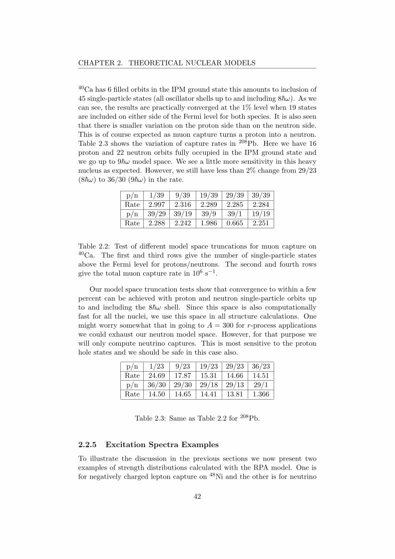
CHAPTER 2. THEORETICAL NUCLEAR MODELS
40Ca has 6 filled orbits in the IPM ground state this amounts to inclusion of45 single-particle states (all oscillator shells up to and including 8~ω). As wecan see, the results are practically converged at the 1% level when 19 statesare included on either side of the Fermi level for both species. It is also seenthat there is smaller variation on the proton side than on the neutron side.This is of course expected as muon capture turns a proton into a neutron.Table 2.3 shows the variation of capture rates in 208Pb. Here we have 16proton and 22 neutron orbits fully occupied in the IPM ground state andwe go up to 9~ω model space. We see a little more sensitivity in this heavynucleus as expected. However, we still have less than 2% change from 29/23(8~ω) to 36/30 (9~ω) in the rate.
p/n 1/39 9/39 19/39 29/39 39/39Rate 2.997 2.316 2.289 2.285 2.284p/n 39/29 39/19 39/9 39/1 19/19Rate 2.288 2.242 1.986 0.665 2.251
Table 2.2: Test of different model space truncations for muon capture on40Ca. The first and third rows give the number of single-particle statesabove the Fermi level for protons/neutrons. The second and fourth rowsgive the total muon capture rate in 106 s−1.
Our model space truncation tests show that convergence to within a fewpercent can be achieved with proton and neutron single-particle orbits upto and including the 8~ω shell. Since this space is also computationallyfast for all the nuclei, we use this space in all structure calculations. Onemight worry somewhat that in going to A = 300 for r-process applicationswe could exhaust our neutron model space. However, for that purpose wewill only compute neutrino captures. This is most sensitive to the protonhole states and we should be safe in this case also.
p/n 1/23 9/23 19/23 29/23 36/23Rate 24.69 17.87 15.31 14.66 14.51p/n 36/30 29/30 29/18 29/13 29/1Rate 14.50 14.65 14.41 13.81 1.366
Table 2.3: Same as Table 2.2 for 208Pb.
2.2.5 Excitation Spectra Examples
To illustrate the discussion in the previous sections we now present twoexamples of strength distributions calculated with the RPA model. One isfor negatively charged lepton capture on 48Ni and the other is for neutrino
42

CHAPTER 2. THEORETICAL NUCLEAR MODELS
capture on 208Pb. The former nucleus is an example of a doubly-magicZ > N nuclei. It lies beyond the proton drip line and is particle unstable.The latter is the standard example of a heavy nucleus. The magic neutronand proton numbers in both nuclei lead us to expect an accurate RPA results,even without the use of partial occupancies. Notice that the direction of theprocesses we consider are ∆Tz = 1 for Z > N and ∆Tz = −1 for N > Z,leaving the GT and Fermi transitions unblocked so that we should see themajor part of the strength in these reactions.
Figure 2.2: Strength distributions as a function of energy (in MeV) for 48Ni (left)and 208Pb (right). The top part gives the 0+ (Fermi) strength, the middle givesthe 1+ (GT) strength, and the bottom shows the J = 1− multipole strength.
In figure (2.2) we present the strength distributions for the 0+ (upperpart, denoted SF)) and the 1+ response (middle part, denoted SGT). 10
These were calculated at non-zero momentum transfer so the sum rulesdiscussed in section (2.2.2) are in principal modified. However, we still findthem to be fulfilled to better than 1%, indicating that the modifications aresmall in these examples. In the lower part of the figure we give the strengthfor the 1− forbidden transition (mainly the spin-dipole term: ~r ∧ ~σ). The
10The figures give the discrete states calculated in the RPA. A real experiment wouldof course produce a smooth distribution due to finite resolution.
43
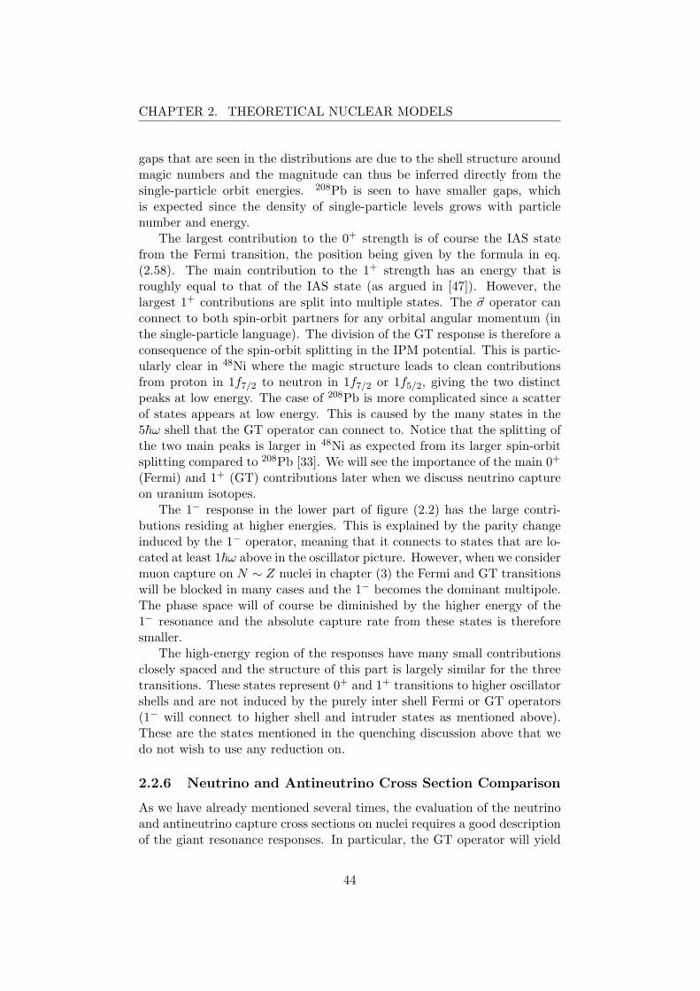
CHAPTER 2. THEORETICAL NUCLEAR MODELS
gaps that are seen in the distributions are due to the shell structure aroundmagic numbers and the magnitude can thus be inferred directly from thesingle-particle orbit energies. 208Pb is seen to have smaller gaps, whichis expected since the density of single-particle levels grows with particlenumber and energy.
The largest contribution to the 0+ strength is of course the IAS statefrom the Fermi transition, the position being given by the formula in eq.(2.58). The main contribution to the 1+ strength has an energy that isroughly equal to that of the IAS state (as argued in [47]). However, thelargest 1+ contributions are split into multiple states. The ~σ operator canconnect to both spin-orbit partners for any orbital angular momentum (inthe single-particle language). The division of the GT response is therefore aconsequence of the spin-orbit splitting in the IPM potential. This is partic-ularly clear in 48Ni where the magic structure leads to clean contributionsfrom proton in 1f7/2 to neutron in 1f7/2 or 1f5/2, giving the two distinctpeaks at low energy. The case of 208Pb is more complicated since a scatterof states appears at low energy. This is caused by the many states in the5~ω shell that the GT operator can connect to. Notice that the splitting ofthe two main peaks is larger in 48Ni as expected from its larger spin-orbitsplitting compared to 208Pb [33]. We will see the importance of the main 0+
(Fermi) and 1+ (GT) contributions later when we discuss neutrino captureon uranium isotopes.
The 1− response in the lower part of figure (2.2) has the large contri-butions residing at higher energies. This is explained by the parity changeinduced by the 1− operator, meaning that it connects to states that are lo-cated at least 1~ω above in the oscillator picture. However, when we considermuon capture on N ∼ Z nuclei in chapter (3) the Fermi and GT transitionswill be blocked in many cases and the 1− becomes the dominant multipole.The phase space will of course be diminished by the higher energy of the1− resonance and the absolute capture rate from these states is thereforesmaller.
The high-energy region of the responses have many small contributionsclosely spaced and the structure of this part is largely similar for the threetransitions. These states represent 0+ and 1+ transitions to higher oscillatorshells and are not induced by the purely inter shell Fermi or GT operators(1− will connect to higher shell and intruder states as mentioned above).These are the states mentioned in the quenching discussion above that wedo not wish to use any reduction on.
2.2.6 Neutrino and Antineutrino Cross Section Comparison
As we have already mentioned several times, the evaluation of the neutrinoand antineutrino capture cross sections on nuclei requires a good descriptionof the giant resonance responses. In particular, the GT operator will yield
44
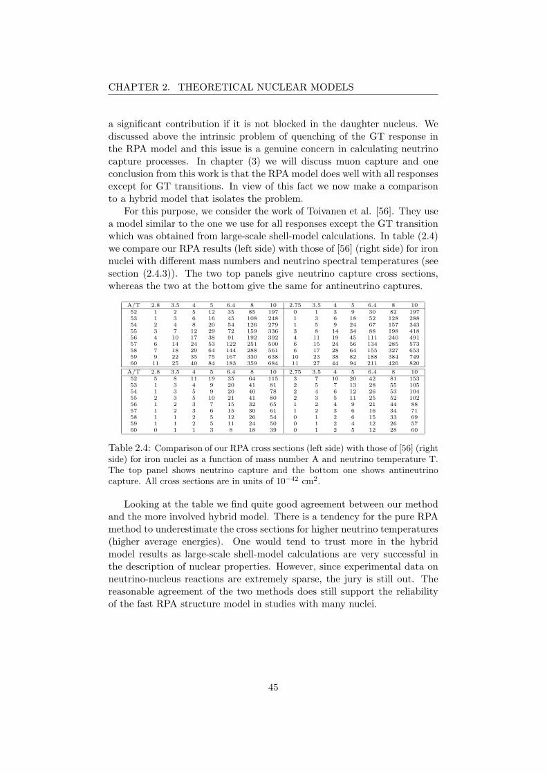
CHAPTER 2. THEORETICAL NUCLEAR MODELS
a significant contribution if it is not blocked in the daughter nucleus. Wediscussed above the intrinsic problem of quenching of the GT response inthe RPA model and this issue is a genuine concern in calculating neutrinocapture processes. In chapter (3) we will discuss muon capture and oneconclusion from this work is that the RPA model does well with all responsesexcept for GT transitions. In view of this fact we now make a comparisonto a hybrid model that isolates the problem.
For this purpose, we consider the work of Toivanen et al. [56]. They usea model similar to the one we use for all responses except the GT transitionwhich was obtained from large-scale shell-model calculations. In table (2.4)we compare our RPA results (left side) with those of [56] (right side) for ironnuclei with different mass numbers and neutrino spectral temperatures (seesection (2.4.3)). The two top panels give neutrino capture cross sections,whereas the two at the bottom give the same for antineutrino captures.
A/T 2.8 3.5 4 5 6.4 8 10 2.75 3.5 4 5 6.4 8 1052 1 2 5 12 35 85 197 0 1 3 9 30 82 19753 1 3 6 16 45 108 248 1 3 6 18 52 128 28854 2 4 8 20 54 126 279 1 5 9 24 67 157 34355 3 7 12 29 72 159 336 3 8 14 34 88 198 41856 4 10 17 38 91 192 392 4 11 19 45 111 240 49157 6 14 24 53 122 251 500 6 15 24 56 134 285 57358 7 18 29 64 144 288 561 6 17 28 64 155 327 65359 9 22 35 75 167 330 638 10 23 38 82 188 384 74960 11 25 40 84 183 359 684 11 27 44 94 211 426 820
A/T 2.8 3.5 4 5 6.4 8 10 2.75 3.5 4 5 6.4 8 1052 5 8 11 19 35 64 115 3 7 10 20 42 81 15353 1 3 4 9 20 41 81 2 5 7 13 28 55 10554 1 3 5 9 20 40 78 2 4 6 12 26 53 10455 2 3 5 10 21 41 80 2 3 5 11 25 52 10256 1 2 3 7 15 32 65 1 2 4 9 21 44 8857 1 2 3 6 15 30 61 1 2 3 6 16 34 7158 1 1 2 5 12 26 54 0 1 2 6 15 33 6959 1 1 2 5 11 24 50 0 1 2 4 12 26 5760 0 1 1 3 8 18 39 0 1 2 5 12 28 60
Table 2.4: Comparison of our RPA cross sections (left side) with those of [56] (rightside) for iron nuclei as a function of mass number A and neutrino temperature T.The top panel shows neutrino capture and the bottom one shows antineutrinocapture. All cross sections are in units of 10−42 cm2.
Looking at the table we find quite good agreement between our methodand the more involved hybrid model. There is a tendency for the pure RPAmethod to underestimate the cross sections for higher neutrino temperatures(higher average energies). One would tend to trust more in the hybridmodel results as large-scale shell-model calculations are very successful inthe description of nuclear properties. However, since experimental data onneutrino-nucleus reactions are extremely sparse, the jury is still out. Thereasonable agreement of the two methods does still support the reliabilityof the fast RPA structure model in studies with many nuclei.
45
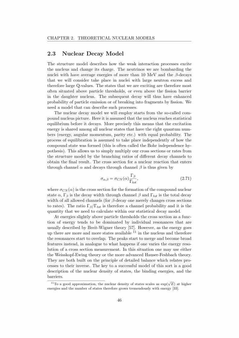
CHAPTER 2. THEORETICAL NUCLEAR MODELS
2.3 Nuclear Decay Model
The structure model describes how the weak interaction processes excitethe nucleus and change its charge. The neutrinos we are bombarding thenuclei with have average energies of more than 10 MeV and the β-decaysthat we will consider take place in nuclei with large neutron excess andtherefore large Q-values. The states that we are exciting are therefore mostoften situated above particle thresholds, or even above the fission barrierin the daughter nucleus. The subsequent decay will thus have enhancedprobability of particle emission or of breaking into fragments by fission. Weneed a model that can describe such processes.
The nuclear decay model we will employ starts from the so-called com-pound nucleus picture. Here it is assumed that the nucleus reaches statisticalequilibrium before it decays. More precisely this means that the excitationenergy is shared among all nuclear states that have the right quantum num-bers (energy, angular momentum, parity etc.) with equal probability. Theprocess of equilibration is assumed to take place independently of how thecompound state was formed (this is often called the Bohr independence hy-pothesis). This allows us to simply multiply our cross sections or rates fromthe structure model by the branching ratios of different decay channels toobtain the final result. The cross section for a nuclear reaction that entersthrough channel α and decays through channel β is thus given by
σα,β = σCN (α)Γβ
Γtot, (2.71)
where σCN (α) is the cross section for the formation of the compound nuclearstate α, Γβ is the decay width through channel β and Γtot is the total decaywidth of all allowed channels (for β-decay one merely changes cross sectionsto rates). The ratio Γβ/Γtot is therefore a channel probability and it is thequantity that we need to calculate within our statistical decay model.
At energies slightly above particle thresholds the cross section as a func-tion of energy tends to be dominated by individual resonances that areusually described by Breit-Wigner theory [57]. However, as the energy goesup there are more and more states available 11 in the nucleus and thereforethe resonances start to overlap. The peaks start to merge and become broadfeatures instead, in analogue to what happens if one varies the energy reso-lution of a cross section measurement. In this situation one may use eitherthe Weisskopf-Ewing theory or the more advanced Hauser-Feshbach theory.They are both built on the principle of detailed balance which relates pro-cesses to their inverse. The key to a successful model of this sort is a gooddescription of the nuclear density of states, the binding energies, and thebarriers.
11To a good approximation, the nuclear density of states scales as exp(√
E) at higherenergies and the number of states therefore grows tremendously with energy [33].
46

CHAPTER 2. THEORETICAL NUCLEAR MODELS
2.3.1 Particle Decay Rates and Fission
We will be using the Weisskopf-Ewing theory [58] for the decay rates. Thisapproach does not take angular momentum changes into account. This isdone in the more advanced Hauser-Feshbach theory. However, we will beconcerned with r-process relevant nuclei that are very neutron-rich so thatessentially only neutron emission and fission contribute, and at low angularmomenta these particular decay modes have little dependence on angularmomentum. Since the neutrino and β-decay reactions populate states withlow J , we will simply ignore the dependence on J and use the Weisskopf-Ewing theory henceforth. The expression for the decay width of a particleevaporation channel a is given by
Γa(Ei) =2Ja + 1ρp(Ei)
ma
π2~2
∫ Ei−Sa
0σa(εa)ρd(Ef )(εa −Ba)dEf , (2.72)
where ρp and ρd are the density of states in the parent and daughter nucleusrespectively and σa is the cross section for the inverse process. The initialenergy, Ei, is the compound nucleus excitation energy, Sa is the bindingenergy of the evaporated particle, and Ba is the barrier in case of chargedparticle evaporation. The integration variable Ef is related to the emittedparticle energy, εa, through εa = Ei − Sa − Ef .
As it stands, this formula contains complicated quantities and we need tointroduce some sensible approximations to make it tractable for calculationsin many different nuclei. To reduce the integral in the width to a simplerform we will use the expression given in [59]. The width formula thenbecomes
Γa(Ei) =2Ja + 1ρp(Ei)
2maR2
π~2T 2
d ρd(Ei − Sa −Ba), (2.73)
where Td is the nuclear temperature in the daughter, defined as the inverselogarithmic derivative of the density of states with respect to energy at themaximum excitation energy in the daughter. R is the nuclear radius, comingfrom the inverse cross section which is approximated by the geometrical one(using the simple radius formula R = 1.4A1/3 fm). To obtain the width fromthis expression we need a solid handle on the density of states in parent anddaughter. We will discuss our choice of this quantity below.
In our r-process considerations we will be particularly concerned withfission. We therefore need a model where this channel is taken into account.The fission decay width will be handled by the transition-state method ofBohr and Wheeler [60]. Using an approximation similar to the one of theprevious section we get [59]
ΓBWfis (Ei) =
Tf
2πρp(Ei)ρd(Ei −Bf ), (2.74)
47
CHAPTER 2. THEORETICAL NUCLEAR MODELS
where Tf is the nuclear temperature in the fissioning parent and Bf is thefission barrier. The barrier is a central quantity and we will discuss it indetail below. In low energy fission there are some known corrections to thisformula. These can be included by multiplication of an enhancement factorthat we get from [61].
Here we should make a cautionary statement. The transition-state modelas given above does not describe the full dynamics of the fission process. Infact, the actual mechanism behind the fragmentation of the nucleus is surelyin the dynamical exchange of energy between excitation degrees of freedomand those of deformation, eventually leading to break-up because of largedistortions in the nuclear shape. The process is one of dissipation of energybetween different degrees of freedom. Such problems are notoriously difficultbut good progress was made in [62] where new analytic approximationswere given for the time-dependence of the fission width that the dissipationcauses. However, at low energies the effects are very small and the puretransition-state model works very well. For this reason we will use theexpression in eq. (2.74) in all our calculations.
Nuclear Binding Energies
The nuclear binding energy is used in virtually all quantities that enter ourwidth calculations. It is therefore pivotal to have a consistent nuclear masscompilation. There are quite a few of these on the market, some of whichare actual tables and some that give analytical formulas from fits. Most ofour calculation will be performed using the finite range liquid-drop (FRDM)model of Moller and Nix [63]. They include corrections for pairing and shells,so that all derived quantities will in principle have these features built in(see however the discussion of fission barriers below). However, to test theuncertainties of our predictions we have also done calculations with massescoming from the Thomas-Fermi model of Myers and Swiatecki [64] that usesthe ground-state shell corrections and pairing energies from [65]. We willleave the discussion of the particulars of each table and specifically theirdifferences until we encounter them when we present our r-process resultsin chapter (6).
Nuclear Density of States
As mentioned above the nuclear density of states is very important for thedetermination of decay widths. We will be using the following general ex-pression
ρ(E) = K1
a1/4E5/4exp
(2√aE), (2.75)
where K is a numerical constant and a is the so-called level density param-eter. In general ρ will also depend on angular momentum and parity, but
48
CHAPTER 2. THEORETICAL NUCLEAR MODELS
in the Weisskopf-Ewing model we neglect this. The level density parameteris known to depend on both nuclear deformation and energy. To incorpo-rate these effects we use the description of Ignatyuk et al. [66, 67]. Thisis based on phenomenology and fits to known experimental data and havebeen proven very robust [68]. We also employ a phenomenological collec-tive enhancement factor that multiplies the state density [69]. In deformednuclei this factor arises because of rotational bands, whereas for sphericalnuclei it is the vibrational states that enhance the density. The theoreticalderivation of such an enhancement factor was given in [70].
Fission Barriers
The question of fission barriers has always been a complicated one. Mea-surements are difficult and have only been performed in a limit number ofnuclei, all of which lie close to the line of β-stability. Calculations involvingnuclei that are far off this line, as is required for r-process applications, haveto rely on semi-empirical or purely theoretical estimates of the barriers. Thismodeling is, however, also very complicated as it consists of determining theminima of nuclear potential energy surfaces which are multidimensional. Asa result, two different barrier compilations can often differ by significantamounts. Realizing this difficulty, we will work with three different choicesfor the barriers as an attempt to estimate these uncertainties.
The first one is that of Sierk [71]. It is based on an early version ofthe FRDM model of Moller and Nix and has the advantage that it allows agood analytical fit. These barriers will be used in conjunction with Mollerand Nix ground-state shell corrections from [65]. The second compilationis the Thomas-Fermi calculations of Myers and Swiatecki [64] that also usethe ground-state shell corrections from [65]. The third choice is the re-cent Extended Thomas-Fermi Strutinsky Integral (ETFSI) method barriersof Mamdouh et al. [72]. This last calculation predicts barriers that risevery steeply at the magic neutron shell around N = 184 which is an im-portant concern in r-process studies, particularly related to the question ofthe maximum mass reached in the process. The ETFSI barriers are severalMeV above the two other compilations in most heavy neutron-rich isotopesso they could drastically change the endpoint. However, a recent study ofthe consistency of different mass compilations have cast some doubt on theETFSI numbers. In [73] the experimental saddle-point masses 12 and fissionbarriers were compared to the predictions of several compilations. This work
12The saddle-point is the boundary point of the nuclear potential where the meta-stableground-state region is separated from the unstable fission region in deformation space.Beyond this point the system will gain energy by splitting into two (or more) fragments.This is merely an easily visualizable 1D definition. In real multi-dimensional potentiallandscapes matters are more complicated. However, the basic picture of the saddle-pointas a boundary of different regions of stability remains.
49
CHAPTER 2. THEORETICAL NUCLEAR MODELS
showed that there are some inconsistencies in the ETFSI predictions, andalso in the Howard and Moller barriers [74] that were used in a number ofprevious studies of the influence of fission on r-process nucleosynthesis. Thebarriers of Sierk, and Myers and Swiatecki did not have these inconsistencies.
2.3.2 Fission Fragments
In the fission process one is of course also interested in the mass and charge ofthe fragments. The theoretical modeling of this issue is another very compli-cated consideration of potential energy surfaces and phase space flows. Theexperimental information is rather sparse and detailed theoretical modelsthat try to reproduce the fragment yields are often only applicable in asmall region of the nuclear chart. The computational efforts involved insuch theoretical descriptions also limit their use. To get a decent handle onthe fragments of many different nuclei it therefore seems reasonable to try asemi-empirical approach. The goals would be to incorporate as much basicphysics of the process as needed and to fit the remaining parameters to theavailable experimental data.
In figure 2.3 we show experimental information on low energy fission dis-tributions for selected nuclei. As is seen in the insets on the figure, there canbe subtle changes in the structure of the fragment distributions. In partic-ular, one sees changes in structure from single- to double- and triple-humpas the mass is increased. Even more intricate is the fact that the actinideshave smooth changes across isotopic chains, whereas the heavier Fermiumisotopes show abrupt changes from double- to single-hump distribution. Anysemi-empirical model that attempts to describe a large number of fissioningsystem has to take these effects into account.
A very successful implementation of such an approach is that of Benlliureet al. [77]. It applies the statistical model to the concept of fission channels.The fragments are determined by the density of states above the potentialenergy surface near the outer saddle-point. This density of states includesthe same pairing, shell and collective effects that were mentioned earlier. Themodel assumes that the potential at the saddle-point can be written in termsof neutron number only. Effects of charge polarization in the fragments aretaken into account later at the scission point. 13 The excitation energy ofthe fragments is also calculated at scission, based on the deformation energyand excitation of the fissioning compound nucleus.
13Naively one would perhaps just assume that the charge distribution would follow thatof the neutrons according to the simple rule Zfrag = Nfrag
Zparent
Nparent. However, deviations
from this expectation are well-known from experiment. This is known as charge polar-ization. Assuming that this degree of freedom equilibrates much faster than the saddle-to-scission time (scission being the point where the two fragments split) it is determinedat the scission point. The actual implementation uses a combination of experimentalinformation and theoretical considerations (see [76] and references therein for details).
50
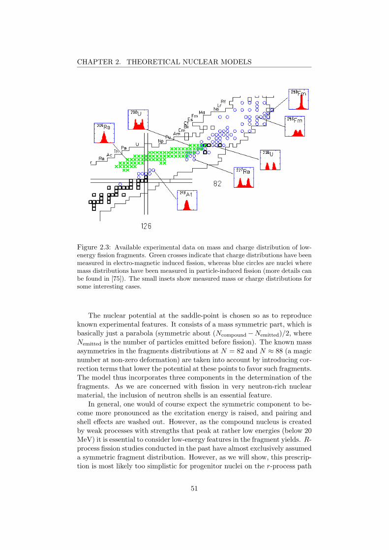
CHAPTER 2. THEORETICAL NUCLEAR MODELS
Figure 2.3: Available experimental data on mass and charge distribution of low-energy fission fragments. Green crosses indicate that charge distributions have beenmeasured in electro-magnetic induced fission, whereas blue circles are nuclei wheremass distributions have been measured in particle-induced fission (more details canbe found in [75]). The small insets show measured mass or charge distributions forsome interesting cases.
The nuclear potential at the saddle-point is chosen so as to reproduceknown experimental features. It consists of a mass symmetric part, which isbasically just a parabola (symmetric about (Ncompound−Nemitted)/2, whereNemitted is the number of particles emitted before fission). The known massasymmetries in the fragments distributions at N = 82 and N ≈ 88 (a magicnumber at non-zero deformation) are taken into account by introducing cor-rection terms that lower the potential at these points to favor such fragments.The model thus incorporates three components in the determination of thefragments. As we are concerned with fission in very neutron-rich nuclearmaterial, the inclusion of neutron shells is an essential feature.
In general, one would of course expect the symmetric component to be-come more pronounced as the excitation energy is raised, and pairing andshell effects are washed out. However, as the compound nucleus is createdby weak processes with strengths that peak at rather low energies (below 20MeV) it is essential to consider low-energy features in the fragment yields. R-process fission studies conducted in the past have almost exclusively assumeda symmetric fragment distribution. However, as we will show, this prescrip-tion is most likely too simplistic for progenitor nuclei on the r-process path
51

CHAPTER 2. THEORETICAL NUCLEAR MODELS
and for the nuclei that decay back toward stability after the r-process freezesout.
2.3.3 The Dynamical Code ABLA
In the previous sections we have described how we will calculate the decaywidth and, in the case of fission, how the fragment distribution is determined.To get a probability distribution for the different decay channels we will beusing a dynamical code called ABLA [78, 77]. It is based on the MonteCarlo principle wherein a random number is used to determine the outcomeof the compound nuclear decay. More concretely, a probability distribution isconstructed based on the widths of all available channels and then a randomnumber is used to determine which channel the nucleus decays into. This ofcourse means that one needs thousands of runs for each nucleus and at allrelevant excitation energies. The parameters that go into the model have tobe easy to compute to maximize the runtime speed. This criterion is metby all quantities described above. Of course a Monte Carlo approach alsoprovides motivation for using the simplest semi-empirical parametrizationthat incorporate the essential physics we want to describe.
One great feature of the ABLA code is that it follows the compounddecay all the way to the ground state. This means that the daughter ofany decay will again be subject to further decays at the relevant excitationenergy (given by energy conservation between parent, daughter, and emittedparticles or fragments). When fission is the outcome the code will evenconsider particles that are evaporated from the fragments. This turns outto be very important for neutron-rich nuclei as we will see later. The decaychain is eventually stopped when the available excitation energy goes belowall particle thresholds. By running this process many times over we thus getprobabilities for emission of particles, and for pre- and post-fission emissionof particles.
The fragment distribution are determined by a subroutine called PROFIthat runs a separate Monte Carlo evaluation. Whenever a fission event isthe outcome of the main routine, PROFI will give two fragments sampledfrom the yields distribution described above. These fragments are thenfed back to the main ABLA routine and allowed to individually decay totheir ground state, possibly through further particle evaporations. In figure2.4 we show a comparison of ABLA calculations and experimental data forfragment charge distributions in actinide nuclei. As can be seen the overallagreement is very good in the observed region.
At our hands we have a robust code that has been thoroughly testedagainst experimental data on heavy nuclei and which incorporates essentialfeatures that are expected to matter in neutron-rich nuclear material. Itprovides us with fission and particle emission probabilities and also fragmentdistributions. We therefore have confidence that ABLA can provide us with
52

CHAPTER 2. THEORETICAL NUCLEAR MODELS
89Ac
90Th
91Pa
92U
131 135134133132 136 137
138 139
140 141
142
Figure 2.4: Comparison of measurements (black dots) and ABLA calculations (redline) of charge distributions in fission fragments from electromagnetically inducedfission on several actinide nuclei in the range 220Ac to 234U shown on a nuclearchart. The distributions are all in the range Z = 24 to Z = 65. Experimental datafrom [75].
valuable information for use in r-process modeling.
2.4 Unified Nuclear Model
We have now described the nuclear structure and the statistical decay modelto be used. Many essential features of how these two models are combinedhave already being introduced in earlier sections. In this section we willrecap the combination for clarity and also comment on various concerns thisprocedure introduces.
In figure 2.5 we present the schematics of the model. The first step ismodeling the nuclear structure of the initial nucleus that is subjected to(anti)neutrino capture or β-decay. For this we need a good handle on theresonances in the 10-20 MeV region in the daughter and also a reasonabledescription of low-lying states. For this we have chosen the RPA method aspreviously described. This method grants us a distribution of cross sectionsor rates for population of the excited states in the daughter nucleus as
53
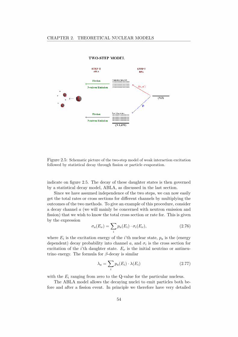
CHAPTER 2. THEORETICAL NUCLEAR MODELS
Figure 2.5: Schematic picture of the two-step model of weak interaction excitationfollowed by statistical decay through fission or particle evaporation.
indicate on figure 2.5. The decay of these daughter states is then governedby a statistical decay model, ABLA, as discussed in the last section.
Since we have assumed independence of the two steps, we can now easilyget the total rates or cross sections for different channels by multiplying theoutcomes of the two methods. To give an example of this procedure, considera decay channel a (we will mainly be concerned with neutron emission andfission) that we wish to know the total cross section or rate for. This is givenby the expression
σa(Eν) =∑
i
pa(Ei) · σi(Eν), (2.76)
where Ei is the excitation energy of the i’th nuclear state, pa is the (energydependent) decay probability into channel a, and σi is the cross section forexcitation of the i’th daughter state. Eν is the initial neutrino or antineu-trino energy. The formula for β-decay is similar
λa =∑
i
pa(Ei) · λ(Ei) (2.77)
with the Ei ranging from zero to the Q-value for the particular nucleus.The ABLA model allows the decaying nuclei to emit particles both be-
fore and after a fission event. In principle we therefore have very detailed
54

CHAPTER 2. THEORETICAL NUCLEAR MODELS
information about the fission decay channel. However, since this all takesplace on the strong interaction timescale there is no point in keeping trackof the emissions relative to the moment of fission. We therefore simplysum these emissions and sum the total number of particles emitted when anucleus undergoes fission.
One of our main concerns is r-process nucleosynthesis, particularly theend-point of this process and the influence of fission. The nuclei that we willbe considering are therefore mostly heavy and neutron-rich. Therefore ourmain decay channels are neutron emission (due to low separation energies)and fission for nuclei with high charge (which often have low fission barriers).
As mentioned in the section on ABLA, the code provides us with dis-tributions for the fragments from fissioning nuclei. These distributions areconstructed by taking all fission events, binning the fragment masses andcharges, and then dividing by the total number of runs for the given nuclei.The yield is simply
Y1(A1, Z1) =N(A1, Z1)
Ntot, (2.78)
where N(A1, Z1) is the number of fragments of mass A1 and charge Z1 andNtot is the total number of Monte Carlo runs. To get the distribution formass or charge alone one simply uses standard probability theory and sumsover the superfluous variable. Generally, the yields depend on energy andthis can be explicitly seen when we compare neutrino-induced processes atdifferent energies in chapter (5).
2.4.1 Energy Mesh
At this point we need to address a technical issue concerning the calculationof decay probabilities using the statistical model. Since it takes the exci-tation energy of the compound nucleus as input, we have to think aboutthe energies at which we employ this model. Obviously we would ideallytake all states and their corresponding energies given to us by the nuclearexcitation structure model and run the decay model with these data. How-ever, since these spectra typically contain hundreds of states scattered belowabout 60-70 MeV with only little prior knowledge about their distributionand strength, this approach would be extremely time-consuming. It is thusclear that a binning of energies must be used in order to achieve our goal ofcalculating many nuclei in a reasonable time frame.
In the present work we have employed the simplest possibility available;the equally spaced energy mesh. This entails calculating the decay proba-bilities for each nucleus on a 1 MeV mesh up to the highest energy nuclearstate. The potential trouble with this choice is concerned with situationswhere a particular channel is opening up. At such a point the probabil-ity changes rather rapidly and the equal mesh can become inadequate. Inparticular, if one uses a model where analytic formulas and experimental
55

CHAPTER 2. THEORETICAL NUCLEAR MODELS
information on the nuclear levels is combined (like the SMOKER code [79])then one would have to be more careful with the energy mesh. However,the ABLA code uses analytic formulae and theoretical mass tables so thisshould be less of a concern. The 1 MeV mesh size was chosen based on testsperformed in selected nuclei demonstrating that a decrease in the mesh sizedid not change the results noticeably.
The nuclear structure model also gives the angular momentum and par-ity of the excited states in the daughter, as was discussed in earlier sections.This can be incorporated in statistical models through a method like Hauser-Feshbach (used in the SMOKER code [79]). As mentioned, the ABLA codeemploys the simpler Weisskopf-Ewing theory, which does not take thesequantum numbers into account. However, the fission barriers used in ABLAare still angular momentum dependent, so we have kept the angular momen-tum information in the combination process. The reactions we consider inthis thesis typically induce excitations with angular momenta J ≤ 4. Thisturns out to be very low on the scale of changes in the J-dependent barriersand letting all state be J = 0 turned out to have virtually no effect on thefinal results. However, the implementation was made J-dependent from thevery beginning and since it did not prolong the calculations noticeably itwas kept in the code. With respect to parity we simply summed over bothvalues for each J and ignored it in the statistical model. Initial investigationinto the changes occurring when parity is taken into account have recentlybeen reported in [80].
2.4.2 Monte Carlo and Statistics
As we have previously discussed, the ABLA code uses Monte Carlo tech-niques to calculate the decay probabilities. Naturally this means that thereis an intrinsic theoretical uncertainty in the calculation. Ideally one has tomake sure that the decay probabilities are converged by varying the numberof runs for each nuclei, excitation energy etc. Of course this is unfeasiblefor the present calculations of thousand of nuclei, so an efficient binning isagain called for.
Initially we have checked the convergence for selected nuclei and exci-tation energies. The general picture that emerged suggested that little wasgained in a change from 10000 to 100000 runs. However, below 10000 therewas some fluctuations in the results. Running the codes with 10000 MonteCarlo runs for each bin and each nuclei would then seem ideal. Unfortu-nately, a quick estimate showed that this would simply take too long. Atthis point we can use the fact that our daughter excitation spectrum rep-resent a distribution. To optimize statistics we thus take into account thepercentage of the cross section or the rate that resides in each energy bin.Making the number of Monte Carlo runs energy dependent in this fashionensures that the important giant resonance states have the best statistics.
56
CHAPTER 2. THEORETICAL NUCLEAR MODELS
This seems to be the best approach available when one does not have muchprior information on the spectral distribution in the decaying nucleus.
2.4.3 Neutrino Spectra and Folding
The formula for the partial cross sections for different decay channels givenabove depends on the energy of the incoming neutrino or antineutrino. In thestellar environment that we are concerned with in this thesis these particleshave certain distributions in energy. Our results are generally functions ofthe neutrino energy and ideally one would like to include the full energydependent cross sections into stellar models. However, for simplicity wewill mostly present total cross sections that are folded with an appropriateneutrino energy distribution to be discussed below.
The theoretical and experimental situation concerning the details ofthese distribution is incredibly rich. This is due to the fact that Super-novae release such an immense amount of energy in the form of neutrinos.The inferences from these spectra therefore hold great promise to reveal de-tails about the nature of this stellar event. Since photons cannot escape theinner parts of this site, neutrinos are actually our only way to obtain thisinformation. In the light of this, it is not surprising that many researcherswork on the imprints of various mechanisms on these spectra and that partof the argument for constructing large neutrino detectors is the prospect ofa galactic Supernova in the near future (estimates show that there shouldbe a little over one event per century). We will not attempt to survey thisvast field, but merely state the details needed for our scenario, commentingon some recent investigations into neutrino oscillations that could have adirect influence on some of the nucleosynthesis results.
We will be working under the assumption that the neutrino spectrumcan be accurately described by a standard Fermi-Dirac energy distribution
f(E, T, µ) = N
[1 + exp
(E − µT
)]−1
, (2.79)
where E is the neutrino energy, T is the temperature, and µ the chemicalpotential of the neutrino species in question. N is a normalization factor thatwe determine below. When addressing the neutrino spectra we will alwaysuse units where all these quantities are measured in MeV. In order to getthe total cross section for a channel a we must fold the energy-dependentquantities of eq. (2.76) with this distribution. This yields
σtota (T, µ) =
∫ ∞
0σ(Eν)af(Eν , T, µ)E2dE. (2.80)
To get the total cross section over all channels we simply sum these partialcross sections over all a. The upper limit on the neutrino energy is taken
57
CHAPTER 2. THEORETICAL NUCLEAR MODELS
to be infinity. This is a good approximation since f(Eν , T, µ) falls off muchfaster than σ(Eν) with energy. However, in actual calculations we need somereasonable cut-off on the integral. As we typically have very little strengthin excited states with energies above about 50 MeV we have used a cut-offvalue of 60 MeV on the neutrino energy, using an equally spaced 1 MeVmesh in all nuclei. 14 To test this choice we have tried going to 100 MeVand found practically no changes in the results.
The fragment distributions also need to take the Fermi-Dirac profile intoaccount when considering neutrino-induced fission events. As mentioned,the fragment yields are energy dependent so we also have to fold these withthe neutrino distribution. To get the mass or charge distributions we simplysum the distributions at each neutrino energy, weight by the Fermi-Diracfactor and then renormalize. The procedure for fission events induced byβ-decays is very similar, only with weighting given by the energy-dependentpartial rate contributions.
The core-collapse Supernova event is perhaps the only place in the Uni-verse where it actually matters that neutrinos are fundamentally fermions.Due to the excessive densities and subsequent neutrino trapping beforebounce, they become degenerate in the inner core and have non-zero chem-ical potential. However, after bounce they diffuse out and are essentiallyfree streaming from beyond a radius known as the neutrino sphere. Sim-ulations show that the expected spectra are not quite Fermi-Dirac but ofa more narrow shape [81, 82]. Having the detailed energy-dependent crosssections would of course principally enable simulation groups to take theexact spectra into account in simulations of neutrino-induced compositionchanges. Such an approach is extremely computationally intensive and onlyvery recently have some groups started to incorporate these. In many casesthe stellar evolution model that gives the neutrino spectra are run indepen-dently of the codes that calculate the subsequent neutrino reactions on theouter layers of the collapsing star. However, quite accurate fits to the spec-tra from detailed evolution codes still display an approximate Fermi-Diracshape with some effective average neutrino energy. We will therefore workunder this assumption throughout.
The above observations have led many subsequent studies to give theaverage energy for the various neutrino species in terms of the thermal Fermi-Dirac distribution. The average energy of a Fermi-Dirac distributed neutrinois easily connected to the temperature parameter T , which is the variableusually given in nucleosynthesis studies where neutrinos are relevant. Weremark that zero chemical potential is most often quite accurate for thespectra and we will assume this from now on. 15 To get the relation between
14This is of course a combined effect of transition matrix elements and phase space. Thelatter grows quadratically with neutrino energy. The exponential fall-off of the Fermi-Diracis, however, strong enough to suppress this effect.
15Simulations of neutrino transport often show that the high-energy tail of the distri-
58
CHAPTER 2. THEORETICAL NUCLEAR MODELS
< E > and T , we first need to normalize f . Integrating over all energieswith a phase space factor of E2dE (since the neutrinos we consider here areultra relativistic) gives∫ ∞
0f(E, T )E2dE = T 3
∫ ∞
0
x2
1 + exp(x)dx. (2.81)
The integral cannot be done analytically, but numerical integration gives1.803. The normalization factor for the distributions is thus 0.5546/T 3. Toget the average energy we must calculate
< E >=∫ ∞
0f(E, T )E3dE =
0.5546T 3
∫ ∞
0
x3
1 + exp(x)dx. (2.82)
This integral is also found when calculating the energy of a photon gas andhas the analytical value 7π4/120. Upon insertion one gets
< E >= 3.15T. (2.83)
We thus see that a factor magically close to π connects energy and temper-ature. This relation allows us to talk about the neutrino temperature andthe average neutrino energy interchangeably.
When addressing the energy or temperature of the out-going neutrinoswe have to be very specific about which species we are talking about. Thetypical temperature of electron neutrinos and antineutrinos are generallynot the same. This feature originates from the fact that the place of lastinteraction (the neutrino sphere) is located at a different radius for the twokinds. Since the material in the protoneutron star is neutron-rich, therewill be more νe on neutron reactions than νe on proton. The antineutrinoswill thus decouple at a smaller radius than the neutrinos. Smaller radiusmeans higher matter temperature and the antineutrinos will therefore havea higher average energy when they stream out. For the µ and τ species theargument is similar, except that these only have neutral current interactions(the charged current cannot contribute due to the large masses of the 2ndand 3rd family leptons). The cross section is generally about 1/6 smallerfor neutral current and we thus have decoupling at an even smaller radiusthan the electron neutrino species.
The typical value for the temperatures of the different species have variedover the years. There has been a tendency for the temperatures to go downslightly as the simulation models become more advanced. Also the energysplitting of different species have become smaller. Some recent values fromcomparisons of different supernova models [83, 84] are
Tνµ ∼ Tνµ ∼ Tντ ∼ Tντ ∼ 8 MeV (2.84)Tνe ∼ 4.5 MeV (2.85)Tνe ∼ 3.5 MeV. (2.86)
bution is weaker than a µ = 0 Fermi-Dirac distribution. This can be effectively taken intoaccount by using non-zero chemical potentials.
59

CHAPTER 2. THEORETICAL NUCLEAR MODELS
The hierarchy discussed above is apparent. 16 The energies given here arefor those neutrinos that emerge from the cooling phase of the protoneutronstar as it equilibrates by releasing excess energy. This process last for aperiod of about 10-20 seconds, during which each species have about equalluminosities. This is not so for earlier stages of the collapse. In particular,around the time of core bounce and shock formation where fluctuations inboth luminosity and average energy are seen. This will be of some concernto us when we discuss the inner-most ejecta but we will postpone the detailsuntil then.
In our studies of r-process nucleosynthesis, we can safely work with thenumbers quoted above as this process takes place some seconds after bounce.The r-process is of course connected to an environment with many freeneutrons and neutron-rich nuclei. We therefore only need to take electronneutrinos into account. We will almost exclusively work with one fixedtemperature of T = 4 MeV, a value that is widely used in previous literature(see for instance [82]). The average energy for this neutrino temperature isabout 12 MeV. This is a rather high energy in nuclear excitation termsand we thus expect to populate the giant resonances discussed in previoussections even for low Q-values. For heavy, neutron-rich nuclei these statesare located at somewhat higher energies of 15 MeV and above, but theconsiderable tail of the Fermi-Dirac distribution and high Q-values still allowpopulation. So we are well within a window of energy where potentiallyinteresting effects of neutrino capture on nuclei can occur.
2.4.4 Anisotropy and Exotica
In this section we will briefly address some of the current topics of greatinterest in Supernova neutrino research. Earlier we have discussed the failureof realistic 1D models to produce consistent Supernova explosions. Theprogress in 2D and 3D simulation codes have now shown that a likely factorin getting successful explosions is convective features that are not presentin the spherically symmetric models (see section (1.3)). Such convectionwould overturn the layers in the star and results in more efficient neutrinoenergy transport. Furthermore, the higher-dimensional models show genericanisotropies in the dynamics. These effects help explode the star, but theycould also be influential in r-process nucleosynthesis in the hot wind abovethe protoneutron star.
The increased energy transport and deposition brought on by convectionwould mean shorter dynamical timescales for the r-process and also help getthe large entropies that are needed to get a high neutron-to-seed ratio. Thiscan be modeled in an effective way by increasing the neutrino luminosities
16A recent study by Keil et al. [85] finds the values 5.5 MeV, 5 MeV, and 4 MeV (withrespect to the order of neutrino species introduced above), indicating that the hierarchyis perhaps less pronounced.
60
CHAPTER 2. THEORETICAL NUCLEAR MODELS
by some factor. One such study was reported in [86] where it was shown toyield consistent r-process nucleosynthesis of the third peak at A ∼ 195. Theneed for multi-D simulations with full transport is once again underlined.These issues should thus be kept in mind later when we explore timescaleand entropy dependencies of our r-process nucleosynthesis calculations inmore detail.
Recently the question of neutrino oscillations was finally settled. The ini-tial findings by John Bahcall and Raymond Davis in their ground-breakingHomestake experiment have been confirmed: Neutrinos undergo flavor os-cillations as they propagate through spacetime. The modern large-scaleexperiments have now given us very detailed information on these oscilla-tions in terms of the mixing angles and the mass squared differences of thevarious species. It is thus not surprising that several studies have looked athow these facts could influence neutrinos in core-collapse Supernovae.
The effect that some people have looked at is the oscillation of the µand τ species into electron neutrino and antineutrinos. The larger averageenergies would then be transfered to a species that can interact with thesurrounding material. This energy boost would enhance cross sections andlead to a stronger energy deposition, possibly helping the explosion of thestar. One early study did find a positive effect on the explosion from thisscenario [87]. The underlying supernova model used in that work is, however,controversial in that it produces explosion in 1D that cannot be reproducedby other studies. The key fact was to have the characteristic length ofoscillation smaller than the gain radius (beyond which neutrinos do not heatthe material). Other studies showed that this length was bigger than thegain radius, providing no help. The parameters needed for the mechanismto work are now known to be inconsistent with experimental bounds onneutrino properties.
Other studies consider the so-called Mikheyev-Smirnov-Wolfenstein ef-fect for resonant oscillations. This effect occurs due to the interaction withthe density of electrons in the stellar environment. Some of the first studiesshowed the effect occurring in Supernova [88]. These parameters were alsofound to be at odds with experimental bounds.
More recently there has been a number of investigations into the effectsof neutrino flavor conversion on nucleosynthesis. The light-element synthesisthat takes place in the outer shells of the star could possibly reside at radiiof roughly the oscillation length and be influenced. Such a study was carriedout in [89] where possible ways to constrain neutrino properties by measuringlight-element abundance ratios was suggested.
For the r-process there could also be an effect if neutrino conversiontakes place. In particular, the effect of so-called active-sterile neutrino os-cillations have been considered. This is connected to the desire of someparticle physics models to add heavy and very weakly interacting neutrinospecies (called sterile) to the Standard Model in order to address certain un-
61
CHAPTER 2. THEORETICAL NUCLEAR MODELS
natural quantities, like the apparent smallness of observed neutrino masses.However, for Supernova applications one needs the sterile neutrinos to belight, something which the LSND experiment suggests could exist. 17 Usingthese light steriles, a consistent r-process nucleosynthesis in the neutrinowind above the protoneutron star was found in a large portion of parameterspace [90, 91].
The possible influence of neutrino conversion through various oscilla-tion scenarios discussed above is something that we will comment on laterin calculations of r-process relevant nuclei. The higher neutrino tempera-tures that would be a result of these mechanisms will of course enhance thecross sections due to simple phase space considerations. We do not expectthe probabilities for neutron emission and fission to change drastically, butthere could be an effect from the fact that fission fragment distributionsare energy-dependent. The larger average neutrino energies could thereforehave an influence on the redistribution of material when fission becomesimportant for the heaviest nuclei at the r-process end-point.
17There is considerable controversy surrounding this experiment as it seems to get differ-ent results from all other experiments that can obtain the same quantities. The follow-upexperiment at Fermilab called MiniBooNE is therefore closely watched and have publishedtheir first results just recently [92]. The initial conclusion goes against the LSND resultsand supports the three light active neutrino species solution.
62
Chapter 3
Muon Capture
3.1 Introduction
We have already mentioned muon capture as a reaction suited for testingnuclear structure models. As discussed above, the main reasons are the rela-tively large amount of energy available for daughter excitation and the largebody of experimental data across the nuclear chart. The study of this semi-leptonic process has a long history and some excellent review articles existby now. Early classics are Mukhopadhyay [94] and Walecka [18], whereasa recent comprehensive review with many experimental details is that ofMeasday [93].
In typical muon capture experiments on not too light nuclei one producesa beam of muons and stop them in a target of the nuclei one would like tomeasure the capture rate on. This requires a trigger telling you when a muonis incident on the target and another trigger to tell you that it was actuallystopped. The former task one can handle with a suitable scintillator. Thestop process is indicated by the emission of gamma rays when the muoncascades down from its initial capture orbit, which has a high Bohr number,to the ground state 1s atomic orbital. This process is electromagnetic andtherefore very fast compared to the nuclear capture governed by the weakinteraction. When a stopped muon is detected, one then starts a timer andwaits for some characteristic signal in the spectrum of the daughter nucleus.In practice, one looks for a gamma ray coming from deexcitation which willalso occur on a short timescale compared to the capture process. The trickis therefore to prepare a good target from the relevant nucleus and to havea good knowledge of the daughter nucleus spectrum for tagging the captureprocess. The experimental techniques for measuring the capture rate havebeen greatly refined over the years and we now have accuracy of a fewpercent in most stable nuclei, excellent data for comparison to theoreticalmodels.
Through the years, there has been a number of theoretical investigations
63

CHAPTER 3. MUON CAPTURE
devoted to global methods for calculating muon capture rates. Papers usinga self-consistent Hartree-Fock random phase approximation scheme similarto the present work have been around for a number of years [95, 96]. Thosestudies found good agreement with experiment, however, only for a limitedselection of nuclei. Capture rates for a broad range of nuclei were also givenin [97]. That study was focused on radiative corrections to the process andthe total capture rates were a by-product which overestimated the experi-mental data. There are also a number of investigations using the simple localFermi gas model [98, 99, 100], where good agreement with measurements fora selection of light, medium and heavy nuclei was found.
To our knowledge, there was not a fully comprehensive calculation of thecapture rates in existence that covered the entire nuclear chart. The goalwas therefore to perform such a global evaluation of the total capture rates.This would constitute a test of our understanding of the nuclear response inthe energy window favored by the process. As we have already pointed outearlier, the capture is dominated by giant resonances at energies up to about30 MeV. More generally, it provides a test of our ability to treat semi-leptonicweak charged-current reactions at momentum transfer q of order the muonmass mµ = 105.6 MeV. Having a good handle on the muon process wouldgive us the needed confidence to proceed with neutrino-nucleus reactionsat similar energetics and momentum transfers, an area where very littleexperimental information is presently available.
3.1.1 Previous Studies
Before we venture into the results obtained during the thesis work we willbriefly discuss the status of our particular model for use in muon capture asof 2003. The work reported here extends the investigations by Kolbe et al.[101, 35]. The first of these papers was concerned with the capture rate in12C, 16O and 40Ca. Here the continuum RPA was used, an extension overthe simple RPA described earlier that takes continuum states into account.Some adjustment to the residual interaction was needed to get agreementwith other observables in carbon and oxygen, but the final results comparedwell with data. Capture rates on a selection of heavier nuclei were considerin the second paper [35]. Apart from an overestimation of the rate in 208Pb,good agreement was again found. This latter paper also showed that onegets almost identical results when using the standard RPA (SRPA) over thecomputationally expensive continuum version. We thus use the former inall calculations presented below. This SRPA approach was already used tostudy nuclear structure effects along isotope chains in Calcium [104] and inNickel and Tin isotopes [34]. These calculations also show good agreementwith the sparse data on isotope effects that exists at the moment.
In figure (3.1) we show an evaluation of the total muon capture rateson all nuclei where data are available and on some heavy nuclei where no
64
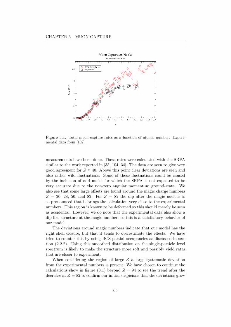
CHAPTER 3. MUON CAPTURE
Figure 3.1: Total muon capture rates as a function of atomic number. Experi-mental data from [102].
measurements have been done. These rates were calculated with the SRPAsimilar to the work reported in [35, 104, 34]. The data are seen to give verygood agreement for Z ≤ 40. Above this point clear deviations are seen andalso rather wild fluctuations. Some of these fluctuations could be causedby the inclusion of odd nuclei for which the SRPA is not expected to bevery accurate due to the non-zero angular momentum ground-state. Wealso see that some large offsets are found around the magic charge numbersZ = 20, 28, 50, and 82. For Z = 82 the dip after the magic nucleus isso pronounced that it brings the calculation very close to the experimentalnumbers. This region is known to be deformed so this should merely be seenas accidental. However, we do note that the experimental data also show adip-like structure at the magic numbers so this is a satisfactory behavior ofour model.
The deviations around magic numbers indicate that our model has theright shell closure, but that it tends to overestimate the effects. We havetried to counter this by using BCS partial occupancies as discussed in sec-tion (2.2.2). Using this smoothed distribution on the single-particle levelspectrum is likely to make the structure more soft and possibly yield ratesthat are closer to experiment.
When considering the region of large Z a large systematic deviationfrom the experimental numbers is present. We have chosen to continue thecalculations show in figure (3.1) beyond Z = 94 to see the trend after thedecrease at Z = 82 to confirm our initial suspicions that the deviations grow
65

CHAPTER 3. MUON CAPTURE
Figure 3.2: As figure (3.1) but as a function of the effective charge (Zeff also from[102]).
with charge. These trends for large Z nuclei led us to suspect that therecould be relativistic effects that were not taken properly into account. Aswe have estimated previously, the muon orbital energy grows with Z2 andcan become a significant fraction of its rest mass in heavy nuclei. However,its orbit radius goes as Z−1 so one should use an effective quantity thatmeasures the charge inside the muon orbit. The effective charge, Zeff ,includes this finite size effect and are tabulated for the (mostly) stable nucleiwe are concerned with here (we have used the values given in [102] whichcites [103] as the original reference). In figure (3.2) we show the rates as afunction of Zeff . This plots confirms that the heaviest nuclei with large Zcause trouble for the current calculations. The closer spacing of data pointsat high Zeff is also of interest. It tells us why the general trend in totalcapture rates shown in figure (3.1) tends to flatten out. Little is gained fromadding protons to heavy nuclei since the core is at saturation and the muoneffective sees only the inner particles.
The main part of our work on muon capture has been devoted to thisrelativistic effect, which will constitute the bulk of this chapter. After work-ing through these modifications, we will comment on other important issuesthat we have attacked along the way. In particular, the issue of quenchingof the GT response and the related discussion of the spin-isospin responseand the parameters of the residual interaction. We round of this chapterwith a presentation and discussion of our results for the capture rate on allmeasured nuclei.
66
CHAPTER 3. MUON CAPTURE
3.2 The Relativistic Muon
When we presented the capture rate formula for muon capture in section(2.1.2), we commented that the muon atomic 1s wave function was a merefactor in the nuclear multipole operators [18]. However, this can be doneonly under the assumption that the muon is essentially non-relativistic sothat its Dirac 4-spinor can be reduced to a radial function times a simple 2-spinor for the muon spin. The radial function can then be found by solving aSchrodinger equation with a potential given by the nuclear charge distribu-tion, which we will also assume is of the standard Woods-Saxon form (usingthe same parameters that went into the calculation of the nuclear single-particle wave functions). For low charges one can use just the constantvalue of the wave function at r = 0, occasionally multiplied by a reductionfactor for finite-size effect [18].
As a first step toward improving this wave function, we have hithertoworked with a radial wave function that came from an actual numericalsolution of the full Dirac equation in the nuclear proton potential. As wediscuss in appendix (A.3), this gives us two radial solutions; a large and asmall component (referring to the non-relativistic limit). However, only thelarge component (that gives the Schrodinger solution in the low-momentumlimit) was used in the rate calculation. As the muon binding energy growswith Z, the small component is expected to become increasingly important.We would therefore like to incorporate it into the muon capture rate formula.
When attempting this, one is immediately faced with a severe problem.In appendix (A.3) one sees that the large (g) and small (f) components donot have the same orbital angular momentum. This can be traced back tothe fact that the Dirac equation does not separately conserve this quantity,only when the spin is added do we get conservation of total angular momen-tum. For g we know that we must have l = 0 since in the low-momentumlimit it must represent the 1s orbit. Since g and f components must differby one unit of orbital angular momentum (appendix (A.3)), this forces fto have l = 1. This is very bad news since it means that the strategy ofmultiplying the nuclear multipole operators by f will destroy their characteras tensor under rotations.
One could start in full generality and consider capture from an arbitraryatomic state into some nuclear states of good angular momenta. Then onewould re-couple the muon wave function with the multipole operators andlet them act in the nuclear Hilbert space. Such derivations were carried outin an older paper by Morita and Fujii [105]. There are, however, a numberof difficulties in the adaption of these results. The paper is written prior tothe advent of the Standard Model of particle physics. At that time, the pureleft-handedness of the neutrino was not an accepted fact. 1 This means that
1Ironically, the recent discovery of neutrino oscillations and mass have yet again started
67

CHAPTER 3. MUON CAPTURE
the out-going neutrino will produce contributions in wave function factorsthat are hard to disentangle when comparing to a more modern treatmentlike that of Walecka [18]. The conventions at that time are also less trans-parent. In particular, the classification of states into allowed, forbidden, 1stforbidden etc. takes a lot of work to translate into the multipole expansionthat we work with. Upon careful consideration, we therefore decided toderive the expressions from scratch in the modern language.
3.2.1 The Leptonic Current
The leptonic part of the current has the standard V-A form
lµ ≡ ψ [γµ (1− γ5)]φ, (3.1)
where ψ is the neutrino and φ is the muon wave function respectively. Theterm (1 − γ5) is the projection operator onto the left-handed componentwhich we need for weak interactions.
The muon wave function comes from the Dirac equation for sphericalpotentials as given in appendix (A.3). Here we will only be concerned withthe capture from the 1s atomic orbit so we immediately specialize the wavefunction to that particular case. The total angular momentum is j = 1/2and this yields the expression
φ1/2 m =(
ig(r)Ω1/2 0 m(r)−f(r)Ω1/2 1 m(r)
), (3.2)
where g(r) and f(r) are the large and small components respectively. Theangular functions have the explicit forms
Ω1/2,0,m = Y0,0(r)χsgn(m) (3.3)
Ω1/2,1,m = −√
3/2−m3 Y1,m−1/2(r)χ+ +
√3/2+m
3 Y1,m+1/2(r)χ−, (3.4)
where χ± are the two-spinor with spin up (+) and down (-). Here we canexplicitly see the appearance of l = 1 terms in the spherical harmonics thatmultiply f(r) and complicate things.
Since the neutrino is not influenced by the interaction of the nucleus itwill have a simple plane wave form. It still has to obey the Dirac equationfor fermions and as such there is a 4-spinor factor to consider. The contentsof this 4-spinor is dictated by the fact that we assume a purely left-handedStandard Model neutrino. This entails a spin that is opposite to the three-momentum. The solution of the Dirac equation with these restrictions can
serious discussions about right-handed neutrino components.
68

CHAPTER 3. MUON CAPTURE
be found in [106]. If we take the momentum ~p along the positive z-axis weget
ψ = N
(χ−−χ−
)exp(i~p · ~x), (3.5)
where χ− are the usual spin down Pauli two-spinors and N is a normalizationconstant (given in appendix (A.1)).
We now have to calculate the leptonic current lµ with these wave func-tions. To keep good tensor properties, we use the standard spherical basisvectors, taking ~e0 = z (appendix (A.2)). The neutrino plane wave has afactor exp(i~p · ~x). With the choice of coordinates one has ~p = kf z = ~q sincethe neutrino moves in the positive z-axis direction. Therefore exp(i~p · ~x) =exp(i~q · ~x). The reason for using the vector ~q is to keep with standard con-ventions for denoting the three-momentum transfer. In our case the muonhas a localized wave function and thus no well-defined three-momentum.From conservation of momentum we therefore conclude that the transferedmomentum is equal to that of the out-going neutrino.
The time component of the lepton current becomes
l0 = ψγ0(1− γ5)φ= ψ†γ2
0(1− γ5)φ= ψ†(1− γ5)φ= ((1− γ5)ψ)†φ= 2ψ†φ, (3.6)
where we have used the fact that the neutrino wave function is left-handedand thus an eigenfunction of (1−γ5). Now we insert the explicit spinor wavefunctions given earlier to get
l0 = 2N∗ exp(−i~q · ~x)(χ †− −χ †
−
)( ig(r)Ω1/2,0,m
−f(r)Ω1/2,1,m
)= 2N∗ exp(−i~q · ~x)
ig(r)χ †
−Ω1/2,0,m + f(r)χ †−Ω1/2,1,m
= 2N∗ exp(−i~q · ~x)
ig(r)Y0,0δm,−1/2 + f(r)
√3/2+m
3 Y1,m+1/2
.
(3.7)
Similarly we get the third component of the lepton current µ = 3 (λ = 0 in
69
CHAPTER 3. MUON CAPTURE
terms of the spherical basis components)
l3 = ψγ3(1− γ5)φ= ψ†γ0γ
3(1− γ5)φ
= ψ†(
0 σz
σz 0
)(1− γ5)φ
= ((
0 σz
σz 0
)ψ)†(1− γ5)φ
= (σzγ5ψ)†(1− γ5)φ= −(σzψ)†(1− γ5)φ= (ψ)†(1− γ5)φ= 2ψ†φ= l0, (3.8)
where σz is always implicitly multiplied by the 4x4 identity. Here we haveused
σz
(χ−−χ−
)=(
σzχ−−σzχ−
)= −
(χ−−χ−
)(3.9)
since the Pauli two-spinors are eigenstates of σz. This equality actuallyfollows straight from current conservation at the lepton vertex, since inmomentum space we have (for massless particles with E = p)
qµlµ = q0l0 − ~q ·~l = q0l0 − ql3 ⇒ l0 = l3. (3.10)
The λ = +1 spherical component of the lepton current is
lλ=+1 = ψ(− 1√2(γ1 + iγ2))(1− γ5)φ
= −√
2ψ†(
0 σ+
σ+ 0
)(1− γ5)φ
= −√
2 ((
0 σ−σ− 0
)ψ)†(1− γ5)φ (3.11)
= 0, (3.12)
where we use the fact that σ−χ− = 0. We see that one spherical componentvanishes which is not surprising since we have an explicitly left/right-handedsymmetry breaking current. The other spherical components is non-zero and
70
CHAPTER 3. MUON CAPTURE
can be evaluated in the same way as above to give
lλ=−1 = ψ( 1√2(γ1 − iγ2))(1− γ5)φ
=√
2ψ†(
0 σ−σ− 0
)(1− γ5)φ
=√
2 ((
0 σ+
σ+ 0
)ψ)†(1− γ5)φ
=√
2N∗ exp(−i~q · ~x)((
0 σ+
σ+ 0
)(χ−−χ−
))†(1− γ5)φ
=√
2N∗ exp(−i~q · ~x)(−χ+
χ+
)†(1− γ5)φ
=√
2N∗ exp(−i~q · ~x)((1− γ5)(−χ+
χ+
))†φ
=√
2N∗ exp(−i~q · ~x)(−2χ+
2χ+
)†φ
= −2√
2N∗ exp(−i~q · ~x)(
χ+
−χ+
)†φ
= −2√
2N∗ exp(−i~q · ~x)(χ †
+ , −χ†
+
)( ig(r)Ω1/2,0,m
−f(r)Ω1/2,1,m
)= −2
√2N∗ exp(−i~q · ~x)ig(r)Y0,0δm,1/2 −
f(r)√
3/2−m3 Y1,m−1/2. (3.13)
We now have the components of the leptonic current in place. Thesehave to be inserted into the interaction hamiltonian
Hint =G√2
∫d3~xjlep
µ Jµnuc =
G√2
∫d3~x
(j0J
0 −~j · ~J). (3.14)
Formally we must take the inner product of this field hamiltonian betweenthe final and initial states which live in the tensor product of nuclear andlepton Hilbert spaces. This we write as
〈f |H|i〉 =G√2
∫d3~x
(l0(~x)J0(~x)fi −~l(~x) · ~J(~x)fi
), (3.15)
whereJµ(~x)fi ≡ 〈fnucleus|Jµ|inucleus〉 (3.16)
is the nuclear current part, which we get from the nuclear structure modeldescribed in chapter (2). We were careful to make sure that the nuclearstates have good total angular momentum and in order not to spoil thisproperty we must be careful when combining the nuclear and lepton parts.
71

CHAPTER 3. MUON CAPTURE
3.2.2 The Non-Relativistic Limit
Before we derive the full expression including large and small muon wavefunction components, we digress to make a sensible consistency check of themethod used. We need to make sure that the formalism introduced abovegives the correct limit when we set f(r) = 0. For convenience (and easy ofcomparison to the formalism in [18]) we first make a slight redefinition ofthe currents to exclude the plane wave exponential factors from the neutrinowave. Thus
l0 → l0 exp(−i~q · ~x)g(r)Y0,0 ⇒ l0 = 2N∗iδm,−1/2
l3 → l3 exp(−i~q · ~x)g(r)Y0,0 ⇒ l3 = 2N∗iδm,−1/2
l+1 = 0l−1 → l−1 exp(−i~q · ~x)g(r)Y0,0 ⇒ l−1 = −2
√2N∗iδ0,1/2, (3.17)
where l±1 are the spherical λ = ±1 components. Now we use the partial waveexpansion of the plane wave (appendix (A.2)) in the interaction hamiltonianto get
H =G√2
∫d3~x exp(−i~q · ~x)g(r)Y0,0l0J0 − l3~e0 · ~J
+∑
λ=±1
lλ~e−λ · ~J
=G√2
∫d3~xg(r)Y0,0l0J0
∞∑J=0
√4π[J ](−i)JjJ(κx)YJ,0
−l3 iκ
∞∑J=0
√4π[J ]∇(jJ(κx)YJ,0) · ~J
+∑
λ=±1
lλ∞∑
J=1
√2π[J ](−i)J [λjJ(κx)~Y−λ
J,J,1 + 1κ∇∧ (jJ(κx)~Y−λ
J,J,1)]
=G√2[∞∑
J=0
√4π[J ](−i)J
M′
J,0l0 − L′J,0l
3
+∑
λ=±1
lλ∞∑
J=1
√2π[J ](−i)J
λJ
′magJ,−1 + J ′el
J,−1
, (3.18)
where the multipole operators are those defined in equations (2.14), (2.15),(2.16), and (2.17). The prime indicates that they are multiplied by g(r)Y00
(which causes no problem with the tensor characters).The assumption of well-defined angular momenta for the nuclear states
allows the use of the Wigner-Eckart theorem [28] to reduce the matrix ele-ments through
〈JfMf |TJ,M |JiMi〉 = (−1)Jf−Mf
(Jf J Ji
−Mf M Mi
)〈Jf ||TJ ||Ji〉 . (3.19)
72
CHAPTER 3. MUON CAPTURE
To get the rate one needs the matrix element squared. Assuming an unpo-larized nucleus, we must average over Mi and sum over Mf . For this we usethe orthogonality relation for the 3-j symbols in the form∑
Mi,Mf
(Jf J Ji
−Mf M Mi
)(Jf J ′ Ji
−Mf M ′ Mi
)=
12J + 1
δJ,J ′δM,M ′ .
(3.20)Using this we get the squared matrix element (there is no interference be-tween the two sums as they have different values of M)
12Ji + 1
∑Mi,Mf
| 〈f |H|i〉 |2 =1
2Ji + 1G2
2[4π|l0|2
∞∑J=0
∣∣∣⟨Jf ||M′J − L
′J ||Ji
⟩∣∣∣2+
∑λ=±1
lλ(lλ)∗∞∑
J=1
∣∣∣⟨Jf ||λJ′magJ + J ′el
J ||Ji
⟩∣∣∣2].(3.21)
At this point we can use the following identity for the spherical components∑λ=±1
lλ(lλ)∗ |a+ λb|2 = (~l · (~l)∗ − l3(l3)∗)(|a|2 + |b|2)− i(~l ∧ (~l)∗)3 2Re(a∗b),
(3.22)where a and b are any complex numbers (this is easily shown by using thedefinition the spherical basis given in appendix (A.2)). We thus need thecartesian components of ~l to use the formula. Since λ = +1 vanishes, thetransformation is easily done. The result is
l0 = l3 = lz = 2N∗iδm,−1/2 lx = −2N∗iδm,1/2 l
y = ilx = 2N∗δm,1/2. (3.23)
The quantities we need above are therefore
~l · (~l)∗ − l3(l3)∗ = 8|N |2δm,1/2 (3.24)(~l ∧ (~l)∗
)3
= lx(ly)∗ − ly(lx)∗ = −8i|N|2δm,1/2. (3.25)
Inserting this in the matrix element of eq. (3.21) gives∑λ=±1
lλ(lλ)∗ |a+ λb|2 = 8|N|2δm,1/2 |a− b|2 . (3.26)
Using this in the summed matrix element squared gives1
2Ji + 1
∑Mi,Mf
| 〈f |H|i〉 |2 =
12Ji + 1
8π|N|2G2[δm,−1/2
∞∑J=0
∣∣∣⟨Jf ||M′J − L
′J ||Ji
⟩∣∣∣2+δm,1/2
∞∑J=1
∣∣∣⟨Jf ||J′elJ − J
′magJ ||Ji
⟩∣∣∣2]. (3.27)
73

CHAPTER 3. MUON CAPTURE
When averaged over muon spin states m = ±1/2 (assuming an unpolar-ized muon) this gives (with suitable normalization and phase space) thenon-relativistic rate formula given in equation (2.19). So the formalism isconsistent with previous work using only the large component of the muonwave function.
3.2.3 The Relativistic Rate Formula
We now proceed to derive the full relativistic muon capture rate formulawith large and small components included. The interaction hamiltonian hasthe general form
H =G√2
∫d3~xl0J0 − l3~e0 · ~J
+∑
λ=±1
lλ~e−λ · ~J
=G√2
∫d3~xl0J0 − l3~e0 · ~J
+l−1~e1 · ~J, (3.28)
since the λ = +1 components was zero. We now want to consider thecontributions from the leptonic part term by term.
The Time Component l0
From the general expression given earlier we have
l0 = 2N∗ exp(−i~q · ~x)ig(r)Y0,0δm,−1/2 + f(r)
√3/2+m
3 Y1,m+1/2
.
(3.29)
We insert the multipole expansion of the plane wave and obtain∫d3~xl0J0 = 2N∗
∫d3~x
∞∑J=0
√4π[J ](−i)JjJ(κx)YJ,0
×ig(r)Y0,0δm,−1/2 + f(r)
√3/2+m
3 Y1,m+1/2
J0
= 2N∗∞∑
J=0
√4π[J ](−i)Jiδm,−1/2
∫d3~xg(r)Y0,0jJ(κx)YJ,0 J0
+√
3/2+m3
∫d3~xf(r)jJ(κx)YJ,0Y1,m+1/2 J0. (3.30)
The first term is just the old M′ term, whereas the second does not havegood tensor character as it stands. To remedy this we use a product formula
74
CHAPTER 3. MUON CAPTURE
for spherical harmonics to reduce it to a sum of harmonics. The formula is
Yl1,m1Yl2,m2 =∑
k
[l1][l2]√4π[k]
〈l1 l2 k|0 0 0〉 〈l1 l2 k|m1m2m1 +m2〉Yk,m1+m2 ,
(3.31)where k is restricted by the usual triangle rule for l1, l2, and k. Consider nowthe second term in eq. (3.30) above. Here one has l1 = J and l2 = 1, and onewould naively assume the sum over k to be restricted to k = J − 1, J, J + 1.The Clebsch-Gordan 〈l1 l2 k|0 0 0〉, however, restricts this by the conditionthat J + 1 + k must be even. So only k = J − 1 and J + 1 are allowed. Tosimplify our expression we define the following quantities
M′J,M =
∫d3~xg(r)Y0,0jJ(κx)YJ,MJ0 (3.32)
α(ρ, J,m) =√
3/2+m3
√34π
[J ][ρ]〈J 1 ρ|000〉
⟨J 1 ρ|0m+ 1
2 m+ 12
⟩(3.33)
T1(ρ, J, µ) =∫
d3~xf(r)jJ(κx)Yρ,µJ0, (3.34)
where the first is simply the coulomb multipole with the large component.The new tensor containing f(r) has the indicated tensor character (ρ, µ).Remember that the constant α has a dependence on the muon spin projec-tion m. With these definitions and the expansion of the spherical harmonicswe get
∫d3~xl0J0 = 2N∗
∞∑J=0
√4π[J ](−i)Jiδm,−1/2M
′J,0
α(J − 1, J,m+ 1
2
)T1(J − 1, J,m+ 1
2
)+α
(J + 1, J,m+ 1
2
)T1(J + 1, J,m+ 1
2
) (3.35)
for the time component (where it is understood that if any of the first twoarguments in α and T1 are negative the term is zero ). We thus see that thisterm adds another two tensors to the general matrix element.
The Third Component l3
The third component of the current (λ = 0 component in spherical notation)is more complicated since it contains a derivative that we have to expandand re-couple. As we have previously seen, the leptonic current is the sameas that of the time component
l3 = 2N∗ exp(−i~q · ~x)ig(r)Y0,0δm,−1/2 + f(r)
√3/2+m
3 Y1,m+1/2
. (3.36)
75

CHAPTER 3. MUON CAPTURE
Using the multipole expansion of the exponential factor one gets∫d3~xl3~e0 · ~J = 2N∗
∫d3~x
i
κ
∞∑J=0
√4π[J ](−i)J∇ (jJ(κx)YJ,0) · ~J
×ig(r)Y0,0δm,−1/2 + f(r)
√3/2+m
3 Y1,m+1/2
= 2N∗
∑∞J=0
√4π[J ](−i)Jiδm,−1/2
∫d3~xg(r)Y0,0∇ (jJ(κx)YJ,0) · ~J
+√
3/2+m3
∫d3~xf(r)∇ (jJ(κx)YJ,0)Y1,m+1/2 · ~J. (3.37)
The last term with f(r) is again not a good tensor. To remedy this weexpand the gradient using the identity (appendix (A.2))
∇ρ (jJ(ρ)YJ,M (Ωρ)) =
√J + 12J + 1
jJ+1(ρ)~YMJ,J+1,1 +
√J
2J + 1jJ−1(ρ)~YM
J,J−1,1.
This turns the problem into a reduction of the product Y1,µ~YM
ρ,γ,1. Using thedefinition of the vector spherical harmonic one has
Y1,µ~YM
J,L,1 =∑m
〈LJ 1|mM −mM〉YL,mY1,µ~eM−m.
First we reduce the product of spherical harmonics by using
Y1,µYL,m =∑
ρ
√34π
[L][ρ]〈1Lρ|0 0 0〉 〈1Lρ|µmµ+m〉Yρ,µ+m.
Now we want to relate the product ~eλYl,m to the vector spherical harmonicby using inversion of the Clebsch-Gordan coefficients (appendix (A.2))
~eλYl,m =∑
γ
〈l 1 γ|mλm+ λ〉 ~Ym+λγ,l,1 ,
where the sum over γ is restricted to γ = l − 1, l, l + 1. Inserting theseformulae gives
Y1,µ~YM
J,L,1 =∑
ρ,γ,m
√34π
[L][ρ]〈1Lρ|000〉 〈1Lρ|µmµ+m〉
× 〈L 1 J |mM −mM〉 〈ρ 1 γ|µ+mM −mM + µ〉 ~YM+µγ,ρ,1 .
We can reduce the expression by using the following relation between theClebsch-Gordan coefficients and the Racah W symbols (which can be foundin [107] or [28])∑
m
〈1Lρ|µmµ+m〉 〈ρ 1 γ|µ+mM −mM + µ〉 〈L 1 J |mM −mM〉
= [J ][ρ]W (1Lγ 1; ρ J) 〈1 J γ|µM M + µ〉 .
76
CHAPTER 3. MUON CAPTURE
When inserting this we finally have the formula for the product
Y1,µ~YM
J,L,1 =∑ρ,γ
√34π [J ][L]W (1Lγ 1; ρ J) 〈1 J γ|µM M + µ〉
× 〈1Lρ|000〉 ~YM+µγ,ρ,1 . (3.38)
The presence of the W coefficient gives us four triangle relations; ∆ (1Lγ),∆ (1 ρ J), ∆ (1LJ) and ∆ (1 ρ γ), which restrict the sum over ρ and γ forgiven J and L. The last Clebsch-Gordan gives us the triangle ∆ (1Lρ), sothat L+ 1 + ρ must be even.
We now expand the f(r) term to get∫d3~x
i
κ
∞∑J=0
√4π[J ](−i)Jf(r)
√3/2+m
3 Y1,m+1/2
×κ
√J + 12J + 1
jJ+1(ρ)~Y0J,J+1,1 +
√J
2J + 1jJ−1(ρ)~Y0
J,J−1,1
= i∞∑
J=0
√4π(−i)J
√3/2+m
3 √J + 12J + 1
∫d3~xf(r)jJ+1(κx)Y1,m+1/2
~Y0J,J+1,1 +√
J
2J + 1
∫d3~xf(r)jJ−1(κx)Y1,m+1/2
~Y0J,J−1,1, (3.39)
where the factor of κ in the numerator comes from the fact that the Besselfunctions depend on ρ = κx, which gives dρ
dx = κ. We now insert thereduction formula derived above in the first term and get√
3/2+m3
√J + 12J + 1
∫d3~xf(r)jJ+1(κx)
∑ρ,γ
√34π [J ][J + 1]
×W (1 J + 1 γ 1; ρ J)⟨1 J γ|m+ 1
2 0m+ 12
⟩〈1 J + 1 ρ|000〉 ~Ym+1/2
γ,ρ,1 .
The last Clebsch-Gordan restricts ρ + J + 2 to an even integer. Thus ρ =J, J + 2 are the only allowed values. γ is obtained by coupling ρ and 1, sonaively γ = ρ − 1, ρ, ρ + 1. However, we have a triangle ∆ (1J + 1 γ) fromW , which does not allow J − 1. Similarly for ρ = J + 2 the value J + 3is not allowed. Lastly we also have ∆ (1 J γ) from W , so that γ = J + 2is ruled out. We therefore have three allowed combinations in the sum:(ρ = J, γ = J − 1), (ρ = J, γ = J), and (ρ = J + 2, γ = J + 1), with therule that whenever ρ or γ is negative the term vanishes. The second term
77

CHAPTER 3. MUON CAPTURE
in equation (3.39) can be treated analogously to yield√3/2+m
3
√J
2J + 1
∫d3~xf(r)jJ−1(κx)
∑ρ,γ
√34π [J ][J − 1]
×W (1 J − 1 γ 1; ρ J)⟨1 J γ|m+ 1
2 0m+ 12
⟩〈1 J − 1 ρ|000〉 ~Ym+1/2
γ,ρ,1 .
Repeating the analysis of allowed terms as done above we get the followingcontributions to the sum: (ρ = J − 2, γ = J − 1), (ρ = J, γ = J − 1), and(ρ = J, γ = J).
We now define the following convenient quantities
L′J,M =
i
κ
∫d3~xg(r)Y0,0∇ (jJ(κx)YJ,M ) J0 (3.40)
β+(γ, ρ,m) =√
3/2+m3
√34π
√J + 1[J + 1] 〈1 J + 1 ρ|000〉
×⟨1 J γ|m+ 1
2 0m+ 12
⟩W (1 J + 1 γ 1; ρ J) (3.41)
T2(γ, ρ, µ) =∫
d3~xf(r)jJ+1(κx)~Yµγ,ρ,1 · ~J (3.42)
β−(γ, ρ,m) =√
3/2+m3
√34π
√J [J − 1] 〈1 J − 1 ρ|000〉
×⟨1 J γ|m+ 1
2 0m+ 12
⟩W (1 J − 1 γ 1; ρ J) (3.43)
T3(γ, ρ, µ) =∫
d3~xf(r)jJ−1(κx)~Yµγ,ρ,1 · ~J, (3.44)
where the two tensors T2, T3 have character (γ, µ). Using these definitionswe can write the contribution from the third component as∫
d3~xl3~e0 · ~J = 2N∗∞∑
J=0
√4π[J ](−i)J iδm,−1/2L
′J,0
+β+(J, J,m)T2(J, J,m+ 12)
+β+(J + 1, J,m)T2(J + 1, J,m+ 12)
+β+(J + 1, J + 2,m)T2(J + 1, J + 2,m+ 12)
+β−(J − 1, J − 2,m)T3(J − 1, J − 2,m+ 12)
+β−(J − 1, J,m)T3(J − 1, J,m+ 12)
+β−(J, J,m)T3(J, J,m+ 12), (3.45)
where it is understood that for a term to give a non-zero contribution thefirst two arguments must be non-negative.
The λ = −1 Component
The leptonic part of this component has the form
lλ=−1 = −2√
2N∗ exp(−i~q · ~x)ig(r)Y0,0δm,1/2 − f(r)√
3/2−m3 Y1,m−1/2.
(3.46)
78

CHAPTER 3. MUON CAPTURE
Inserting the multipole expansion of the plane wave yields∫d3~xl−1~e1 · ~J = −2N∗
∫d3~x
∞∑J=1
√4π[J ](−i)J [−jJ(κx)~Y1
J,J,1
+ 1κ∇∧ (jJ(κx)~Y1
J,J,1)] · ~J
×ig(r)Y0,0δm,1/2 − f(r)
√3/2−m
3 Y1,m−1/2
= −2N∗
∞∑J=1
√4π[J ](−i)Jiδm,1/2
∫d3~xg(r)Y0,0
×[−jJ(κx)~Y1J,J,1 + 1
κ∇∧ (jJ(κx)~Y1J,J,1)]
+√
3/2−m3
∫d3~xf(r)jJ(κx)~Y1
J,J,1Y1,m−1/2
−√
3/2−m3
∫d3~xf(r)∇∧ (jJ(κx)~Y1
J,J,1)Y1,m−1/2 · ~J.
(3.47)
The first two terms are simply the transverse magnetic and electric multipoleoperators of eqs. (2.16) and (2.17) with the large component included
J ′elJ,M =
1κ
∫d3~xg(r)Y0,0∇∧
(jJ(κx)~YM
J,J,1
)· ~J (3.48)
J′magJ,M =
∫d3~xg(r)Y0,0jJ(κx)~YM
J,J,1 · ~J. (3.49)
The first of the terms involving f(r) can be handled using the same meth-ods as for the third component above. Reduction of the product of vectorspherical and spherical harmonic yields√
3/2−m3
∫d3~xf(r)jJ(κx)
∑ρ,γ
√34π [J ]2W (1 J γ 1; ρ J)
×⟨1 J γ|m− 1
2 1m+ 12
⟩〈1 J ρ|000〉 ~Ym+1/2
γ,ρ,1 .
Since ρ+J +1 must be even only ρ = J − 1, J +1 are allowed. The trianglerelations coming from the W coefficient give the conditions γ = J−1, J, J+1and γ = ρ− 1, ρ, ρ+ 1. Taking all this into account restricts the sum to thefollowing terms: (ρ = J−1, γ = J−1), (ρ = J−1, γ = J), (ρ = J+1, γ = J),and (ρ = J + 1, γ = J + 1). Defining the quantities
δ(γ, ρ,m) =√
3/2−m3
√34π [J ]2 〈1 J ρ|000〉 (3.50)
×⟨1 J γ|m− 1
2 1m+ 12
⟩W (1 J γ 1; ρ J) (3.51)
T4(γ, ρ, µ) =∫
d3~xf(r)jJ(κx)~Yµγ,ρ,1 · ~J, (3.52)
79

CHAPTER 3. MUON CAPTURE
the allowed terms become
δ(J − 1, J − 1,m)T4(J − 1, J − 1,m+ 12)
δ( J , J − 1,m)T4( J , J − 1,m+ 12)
δ( J , J + 1,m)T4( J , J + 1,m+ 12)
δ(J + 1, J + 1,m)T4(J + 1, J + 1,m+ 12).
For the second term containing f(r) we need to expand the cross prod-uct by using the identity given in appendix (A.2). Multiplying by 1
κ andremembering that the differentiation gives a factor κ, we arrive at
1κ∇∧
(jJ(κx)~YM
J,J,1
)= −i
√J
2J+1jJ+1(κx)~YMJ,J+1,1
+i√
J+12J+1jJ−1(κx)~YM
J,J−1,1.
The analysis of these terms can be carried out in complete analogy to theprevious ones so we skip the details. It is convenient to define some finalquantities before giving the general expression for this part of the current.We introduce
η+(γ, ρ,m) =√
3/2−m3
√34π
√J [J + 1] 〈1 J + 1 ρ|000〉
×⟨1 J γ|m− 1
2 1m+ 12
⟩W (1 J + 1 γ 1; ρ J) (3.53)
η−(γ, ρ,m) =√
3/2−m3
√34π
√J + 1[J − 1] 〈1 J − 1 ρ|000〉
×⟨1 J γ|m− 1
2 1m+ 12
⟩W (1 J − 1 γ 1; ρ J) . (3.54)
There is no need to define new tensors at this point as the ones that arisehere are simply T2 and T3 introduced above. Putting everything together weend up with the following rather lengthy expression for the λ = −1 spherical
80
CHAPTER 3. MUON CAPTURE
component of the current∫d3~xl−1~e1 · ~J = 2N∗
∞∑J=1
√4π[J ](−i)Jiδm,1/2
J ′el
J,1 − J′magJ,1
−δ(J − 1, J − 1,m)T4(J − 1, J − 1,m+ 1
2)−δ(J, J − 1,m)T4(J, J − 1,m+ 1
2)−δ(J, J + 1,m)T4(J, J + 1,m+ 1
2)−δ(J + 1, J + 1,m)T4(J + 1, J + 1,m+ 1
2)+iη+(J, J,m)T2(J, J,m+ 1
2)+iη+(J + 1, J,m)T2(J + 1, J,m+ 1
2)+iη+(J + 1, J + 2,m)T2(J + 1, J + 2,m+ 1
2)−iη−(J − 1, J,m)T3(J − 1, J,m+ 1
2)−iη−(J, J,m)T3(J, J,m+ 1
2)−iη−(J − 1, J − 2,m)T3(J − 1, J − 2,m+ 1
2).(3.55)
81

CHAPTER 3. MUON CAPTURE
The Full Interaction Hamiltonian
We now summarize the derivation by giving the full relativistic hamiltonian.It has the lengthy expression
H =G√2
∫d3~xl0J0 − l3~e0 · ~J + l−1~e1 · ~J
=2GN∗√
2[∞∑
J=0
√4π[J ](−i)Jiδm,−1/2
M′
J,0 − L′J,0
+α
(J − 1, J,m+ 1
2
)T1(J − 1, J,m+ 1
2
)+α
(J + 1, J,m+ 1
2
)T1(J + 1, J,m+ 1
2
)−iβ+(J, J,m)T2(J, J,m+ 1
2)−iβ+(J + 1, J,m)T2(J + 1, J,m+ 1
2)−iβ+(J + 1, J + 2,m)T2(J + 1, J + 2,m+ 1
2)−iβ−(J − 1, J − 2,m)T3(J − 1, J − 2,m+ 1
2)−iβ−(J − 1, J,m)T3(J − 1, J,m+ 1
2)−iβ−(J, J,m)T3(J, J,m+ 1
2)
+∞∑
J=1
√4π[J ](−i)Jiδm,1/2
J ′el
J,1 − J′magJ,1
−δ(J − 1, J − 1,m)T4(J − 1, J − 1,m+ 1
2)−δ(J, J − 1,m)T4(J, J − 1,m+ 1
2)−δ(J, J + 1,m)T4(J, J + 1,m+ 1
2)−δ(J + 1, J + 1,m)T4(J + 1, J + 1,m+ 1
2)+iη+(J, J,m)T2(J, J,m+ 1
2)+iη+(J + 1, J,m)T2(J + 1, J,m+ 1
2)+iη+(J + 1, J + 2,m)T2(J + 1, J + 2,m+ 1
2)−iη−(J − 1, J,m)T3(J − 1, J,m+ 1
2)−iη−(J, J,m)T3(J, J,m+ 1
2)−iη−(J − 1, J − 2,m)T3(J − 1, J − 2,m+ 1
2)]. (3.56)
This hamiltonian is truly a horrible piece of formalism! In order to reduceit to something that is more convenient when trying to group the terms, we
82

CHAPTER 3. MUON CAPTURE
now make another round of definitions.
X 1(J, 0) = iδm,−1/2
M′
J,0 − L′J,0
(3.57)
X 2(J − 1,m+ 12) = α
(J − 1, J,m+ 1
2
)T1(J − 1, J,m+ 1
2
)−iβ−(J − 1, J − 2,m)T3(J − 1, J − 2,m+ 1
2)−iβ−(J − 1, J,m)T3(J − 1, J,m+ 1
2) (3.58)X 3(J,m+ 1
2) = −iβ+(J, J,m)T2(J, J,m+ 12)
−iβ−(J, J,m)T3(J, J,m+ 12) (3.59)
X 4(J + 1,m+ 12) = α
(J + 1, J,m+ 1
2
)T1(J + 1, J,m+ 1
2
)−iβ+(J + 1, J,m)T2(J + 1, J,m+ 1
2)−iβ+(J + 1, J + 2,m)T2(J + 1, J + 2,m+ 1
2)(3.60)
Z1(J, 1) = iδm,1/2
J ′el
J,1 − J′magJ,1
(3.61)
Z2(J − 1,m+ 12) = −δ(J − 1, J − 1,m)T4(J − 1, J − 1,m+ 1
2)−iη−(J − 1, J,m)T3(J − 1, J,m+ 1
2)−iη−(J − 1, J − 2,m)T3(J − 1, J − 2,m+ 1
2)(3.62)
Z3(J,m+ 12) = −δ(J, J − 1,m)T4(J, J − 1,m+ 1
2)−δ(J, J + 1,m)T4(J, J + 1,m+ 1
2)−iη−(J, J,m)T3(J, J,m+ 1
2) (3.63)Z4(J + 1,m+ 1
2) = −δ(J + 1, J + 1,m)T4(J + 1, J + 1,m+ 12)
+iη+(J + 1, J,m)T2(J + 1, J,m+ 12)
+iη+(J + 1, J + 2,m)T2(J + 1, J + 2,m+ 12).(3.64)
These terms have the advantage that they have the tensor character (J,M)indicated in the parenthesis. One must, however, remember that the con-stants in these expressions depend explicitly on m. The above quantities cannow be inserted into the hamiltonian. However, each of these is non-zeroonly when the angular momentum is non-negative. To ease the applicationof the Wigner-Eckart theorem in squaring the matrix element, it is advanta-geous to change the bounds on the sums over angular momenta. This yields
83

CHAPTER 3. MUON CAPTURE
the following more compact hamiltonian
H =2GN∗√
2[∞∑
J=0
√4π[J ](−i)J
X 1(J, 0) + X 3(J,m+ 1
2)
+∞∑
J=0
√4π[J ](−i)J
X 4(J + 1,m+ 1
2)
+∞∑
J=1
√4π[J ](−i)J(X 2(J − 1,m+ 1
2) + Z2(J − 1,m+ 12)
+Z1(J, 1) + Z3(J,m+ 12) + Z4(J + 1,m+ 1
2)). (3.65)
We now shift the sums so that all tensors have angular momentum J tomake it simpler to calculate the interference terms when squaring. Thisyields
H =2GN∗√
2[∞∑
J=0
√4π[J ](−i)J
X 1(J, 0) + X 3(J,m+ 1
2)
+∞∑
J=1
√4π[J − 1](−i)J iX 4(J,m+ 1
2)
+∞∑
J=1
√4π[J ](−i)J
Z3(J,m+ 1
2) + Z1(J, 1)
+∞∑
J=0
√4π[J + 1](−i)J(−i)
X 2(J,m+ 1
2) + Z2(J,m+ 12)
+∞∑
J=2
√4π[J − 1](−i)J iZ4(J,m+ 1
2). (3.66)
The Matrix Element
We need to find the matrix element with the nuclear states of good angu-lar momentum and use the Wigner-Eckart theorem to get reduced matrixelements. For simplicity we introduce the notations
aMJ = (−1)Jf−Mf
(Jf J Ji
−Mf M Mi
)(3.67)
|TJ | = 〈Jf ||TJ ||Ji〉 . (3.68)
The completeness relation for the 3-j symbols is then given by∑Mi,Mf
(aMJ )∗aM ′
J ′ = 12J+1δM,M ′δJ,J ′ = [J ]−2δM,M ′δJ,J ′ . (3.69)
84
CHAPTER 3. MUON CAPTURE
Using these notations, the matrix element becomes (with µ = m+ 12)
〈f |H|i〉 =2GN∗√
2[∞∑
J=0
√4π[J ](−i)J
a0
J |X 1J |+ aµ
J |X3J |
+∞∑
J=1
√4π[J − 1](−i)J−1aµ
J |X4J |
+∞∑
J=1
√4π[J ](−i)J
a1
J |Z1J |+ aµ
J |Z3J |
+∞∑
J=0
√4π[J + 1](−i)J+1
aµ
J |X2J |+ aµ
J |Z2J |
+∞∑
J=2
√4π[J − 1](−i)J−1aµ
J |Z4J |. (3.70)
We assumed an unpolarized nucleus and thus have to average over initialprojection quantum numbers for both nucleus and muon. We also have tosum over final states since we assume that no polarization is measured inthe final state. The quantity we are interested in is thus
12
∑µ=0,1
12Ji + 1
∑Mi,Mf
| 〈f |H|i〉 |2. (3.71)
We notice that for (m = −12 ⇔ µ = 0) we only have interference terms
between X 1 and all the f(r) terms (X i,Zi, i ≥ 2). For (m = 12 ⇔ µ = 1) it
is only Z1 that has these interference terms. Another way to see this is tonotice that the definitions of these leading multipole operators X 1 and Z1
involve δm,±1/2.First we find the terms that contribute for (m = −1/2⇔ µ = 0). There
are a couple of direct terms (same sum in eq. (3.70))
∞∑J=0
|X 1J |2 + 2Re
∞∑J=0
|X 1J |∗|X 3
J |. (3.72)
The other terms give expressions like
2Re∞∑
J=0
∞∑J ′=1
[J ][J ′ − 1](i)J(−i)J ′−1|X 1J |∗|X 4
J |∑
Mi,Mf
(a0J)∗a0
J ′
= 2Re∞∑
J=1
[J − 1][J ]
i|X 1J |∗|X 4
J |. (3.73)
The case with m = 1/2, µ = 1 is analogous. Using these techniques we cannow write down our final expression for the total matrix element in terms
85

CHAPTER 3. MUON CAPTURE
of reduced matrix elements of the various tensor operators. The result is
12
∑µ=0,1
12Ji + 1
∑Mi,Mf
| 〈f |H|i〉 |2 =4πG2|N|2
2Ji + 1[∞∑
J=0
|X 1J |2 +
∞∑J=1
|Z1J |2
+2Re∞∑
J=0
|X 1J |∗|X 3
J |+∞∑
J=0
[J + 1][J ]
(−i)|X 1J |∗(|X 2
J |+ |Z2J |)
+∞∑
J=1
([J − 1]
[J ]i|X 1
J |∗|X 4J |+ |X 1
J |∗|Z3J |+ |Z1
J |∗(|X 3
J |+ |Z3J |))
+∞∑
J=2
[J − 1][J ]
i(|X 1
J |∗ + |Z1J |∗)|Z4
J |
+∞∑
J=1
[J + 1][J ]
(−i)|Z1J |∗(|X 2
J |+ |Z2J |)
+∞∑
J=1
[J − 1][J ]
i|Z1J |∗|X 4
J |
+∑
µ=0,1
[∞∑
J=0
([J + 1]2
[J ]2|X 2
J |2 + |Z2J |2+ |X 3
J |2 + |Z3J |2)
+∞∑
J=1
[J − 1]2
[J ]2|X 4
J |2 +∞∑
J=2
[J − 1]2
[J ]2|Z4
J |2
+∑
µ=0,1
2Re∞∑
J=1
[J − 1][J + 1][J ]2
(−i)2|X 4J |∗[|X 2
J |+ |Z2J |]
+∞∑
J=2
[[J − 1]2
[J ]2|X 4
J |∗|Z4J |+
[J − 1][J + 1][J ]2
(i)2|Z4J |∗(|X 2
J |+ |Z2J |)]
+∞∑
J=1
[[J − 1]
[J ]i|X 3
J |∗|X 4J |+ |X 3
J |∗|Z3J |]
+∞∑
J=2
[J − 1][J ]
i[|X 3
J |∗|Z4J |+ |Z3
J |∗|Z4J |]
+∞∑
J=1
[[J − 1]
[J ]i|Z3
J |∗|X 4J |+
[J + 1][J ]
(−i)|Z3J |∗(|X 2
J |+ |Z2J |)]
+∞∑
J=0
[J + 1][J ]
(−i)|X 3J |∗[|X 2
J |+ |Z2J |]]. (3.74)
The first two terms are those that contain only the large component g(r).The next block are the interference terms of multipoles with g(r) and f(r)respectively. After that we have the terms with only f(r). There are bothdirect and interference terms coming from the latter, since they are presentfor both values of µ. We must remember that the constants that we havedefined through this derivation depend explicitly on m or µ = m+ 1/2. Inthe first block of interference terms we can get the value of µ by looking
86
CHAPTER 3. MUON CAPTURE
at whether the term multiplies an X 1 or a Z1 factor. The former is onlypresent for µ = 0, whereas the latter exists only for µ = 1. For the otherterms we have simply kept the sum over µ.
Evaluation of the Tensor Terms
To arrive at the expression for the matrix element given above, we introducedfour new tensors in addition to the four that we gave in eqs. (2.14), (2.15),(2.16), and (2.17). They were defined by
T1(ρ, J, µ) =∫
d3~xf(r)jJ(κx)Yρ,µJ0 (3.75)
T2(γ, ρ, µ) =∫
d3~xf(r)jJ+1(κx)~Yµγ,ρ,1 · ~J (3.76)
T3(γ, ρ, µ) =∫
d3~xf(r)jJ−1(κx)~Yµγ,ρ,1 · ~J (3.77)
T4(γ, ρ, µ) =∫
d3~xf(r)jJ(κx)~Yµγ,ρ,1 · ~J. (3.78)
Notice that the tensors have a dependence on the angular momentum J ontheir spherical Bessel components coming from the multipole expansion ofthe neutrino plane wave.
To implement these new terms in our nuclear model we need to insertthe nuclear current operators and reduce the expressions to single-particlematrix elements, in the same fashion as for the neutrino capture operators insection (2.2.3). The procedure becomes more involved due to the presenceof the muon wave function and the fact that the order of the sphericalBessels are different in the new tensor (as mentioned above). It is, however,a principally straightforward exercise in coupling and recoupling of tensorproducts along the lines of Edmonds [28].
3.3 Quenching of Multipoles
We showed in section (2.2.2) that the RPA model fulfills the sum rules forthe important cases of Fermi and GT transitions. Previous works on muoncapture using the RPA have suggested that no quenching is needed on thenuclear axial-vector coupling GA [101, 35]. As we have stressed severaltimes, the response is dominated by giant resonances at energies of aroundand above 15 MeV (decreasing with mass and charge numbers), so we donot expect to be very sensitive to low energy strength. In addition, the GToperators will contribute very little in heavier nuclei due to Pauli blockingof the states that the GT can connect to, so again we should not be toosensitive to quenching of this operator.
For lighter nuclei there can be contributions at low energy from the GToperator and in order not to overestimate these we use quenching here. In
87
CHAPTER 3. MUON CAPTURE
particular, we have reduced the low energy (up to 15 MeV) part of the 1+
multipole (which is virtually only GT contributions) by the common factor(0.8)2 = 0.64 which is the recommended value [108]. This procedure hasbeen used for all nuclei with N or Z less than 40.
In principle, our calculations here can also tell us about quenching inother multipoles. We have found that no such quenching was needed in orderto get a good reproduction of the experimental data on muon capture. Thisleads us to conclude that inclusive semi-leptonic processes with momentumtransfer of order q ∼ mµ can be described accurately with the unquenchedstrengths of operators other than GT. Higher multipoles generally have theirresonances at higher energies so we can conclude that our model works quitewell for weak interactions on nuclei in a wide energy range. We thus feelconfident that it can also be used for neutrino processes in the same rangeof energy, including the ones that come from Supernovae that will be ourconcern in subsequent chapters.
3.4 The Residual Interaction
A final detail that we have to address before presenting the results, is con-cerned with the parameters of the residual interaction. In section (2.2.2)we have presented the typical parameters of the Landau-Migdal force thatwe use as residual interaction. Since muon capture in most stable nucleisuffers severe Pauli blocking effects, it is dominated by forbidden transitions(higher order spin-isospin operators) and the most important parameter istherefore the spin-isospin coupling g′. We will therefore only discuss g′ inconnection with muon capture, keeping the rest of the parameters fixed atthe values given earlier. 2
In the older recommendations of Rinker and Speth [41] the value g′ = 0.7is given. This was found to be quite good for reproducing the data in lightnuclei such as 12C and 16O [101]. However, the calculations with g′ = 0.7shown in figure (3.1) have obvious problems for heavier nuclei as discussedearlier. Considering the fact that the spin-isospin term is repulsive for thedominant T = 1 and S = 1 term in muon capture on heavy nuclei (the 1+
multipole), a larger g′ pushes strength to higher energies and thus reducesthe rate. So we are in a situation where we seem to need different parametersfor light and heavy nuclei.
Fortunately, the recent review [43] cites a recommended value in heavynuclei of g′ = 0.96. So we have an indication that there could be a massdependence of the coupling. For simplicity (and lack of a better, moreconsistent option), we introduce the following simple interpolation formula
g′ = c1 + c2A1/3. (3.79)
2We have made several investigations into the dependence of the capture rate on theother parameters and have found very little sensitivity.
88

CHAPTER 3. MUON CAPTURE
The constants c1 and c2 are fitted so that g′ = 0.74 in 16O and g′ = 0.96 in208Pb. We now have a mild dependence on nuclear mass in the axial couplingconstant, which introduces about 10% changes in the rate as compared tothe fixed value g′ = 0.7 for all nuclei.
3.5 Results and Discussion
Having discussed all the particular features needed to specify and improveour model for describing muon capture, we are now ready to present theresults of the new rate calculations. We will only be presenting rates foreven-even nuclei since these are (principally) the cases where the model isapplicable. Including odd-even and odd-odd could introduce deviations dueto the J 6= 0 ground-state and we therefore exclude these nuclei to make thecomparison more transparent (we note that the general trends of the dataare reproduced for these cases as well).
Figure 3.3: Comparison between the measured total muon capture rates [102]denoted by squares , the calculated rates with all corrections (empty circles ©),and the calculated rates without the BCS and relativistic corrections (diamonds ♦). The insert, in larger scale, shows the same results for light nuclei. When themeasurements are for the natural abundance of a given element, the calculationrepresent the corresponding combination of the individual isotopes.
In figure (3.3) the total capture rates as a function of charge for all
89
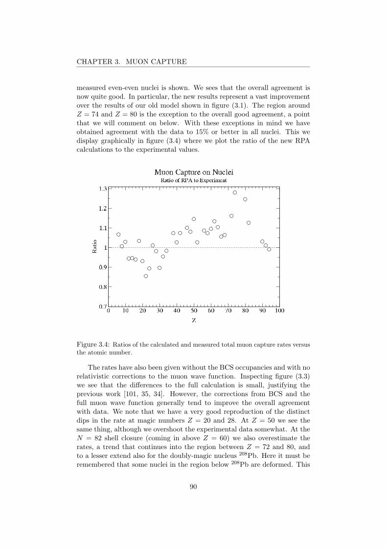
CHAPTER 3. MUON CAPTURE
measured even-even nuclei is shown. We sees that the overall agreement isnow quite good. In particular, the new results represent a vast improvementover the results of our old model shown in figure (3.1). The region aroundZ = 74 and Z = 80 is the exception to the overall good agreement, a pointthat we will comment on below. With these exceptions in mind we haveobtained agreement with the data to 15% or better in all nuclei. This wedisplay graphically in figure (3.4) where we plot the ratio of the new RPAcalculations to the experimental values.
Figure 3.4: Ratios of the calculated and measured total muon capture rates versusthe atomic number.
The rates have also been given without the BCS occupancies and with norelativistic corrections to the muon wave function. Inspecting figure (3.3)we see that the differences to the full calculation is small, justifying theprevious work [101, 35, 34]. However, the corrections from BCS and thefull muon wave function generally tend to improve the overall agreementwith data. We note that we have a very good reproduction of the distinctdips in the rate at magic numbers Z = 20 and 28. At Z = 50 we see thesame thing, although we overshoot the experimental data somewhat. At theN = 82 shell closure (coming in above Z = 60) we also overestimate therates, a trend that continues into the region between Z = 72 and 80, andto a lesser extend also for the doubly-magic nucleus 208Pb. Here it must beremembered that some nuclei in the region below 208Pb are deformed. This
90

CHAPTER 3. MUON CAPTURE
means that the single-particle structure is certainly different from the oneof our spherical mean-field model. We should therefore not expect perfectagreement. When looking at the heaviest nuclei where the rate is knownexperimentally, Th, U, and Pu, we find much better agreement. This is,however, likely a consequence of the dips beyond magic shell closure that wealso saw at lower Z (an effect that was also noted in [111], see in particularFig. 3 of that reference).
As we have noted above, we have used the unquenched axial-vector cou-pling constant for all states, except for the low-energy 1+ contributions, theregion where the Gamow-Teller transition is found. For light- and medium-mass nuclei the dominant multipole is the spin-dipole 1− operator (and toa lesser extent also the quadrupole-like 2+ multipole). Our results thus in-dicate that no quench is needed for these operators. However, for heaviernuclei like 208Pb and beyond we get significant contributions from the 1+
transition. The neutron excess of these nuclei completely block the pureGT operator and the 1+ in this case corresponds to a transition across twomajor oscillator shells, a 2~ω mode. The relatively good agreement withdata thus supports absence of quenching for such modes.
Figure 3.5: Centroids for 1+ (black squares), 1− (red circles), and 2− (blue tiltedsquares) multipole responses as a function of the charge Z. The centroids arecalculated from < E >=
∑f λfEf/λtot, where the sum is over all states f that
contribute to the particular multipole, λf is the partial rate of the state f , and Ef
is the energy of this state in the daughter. λtot is the total rate for the multipole.
91

CHAPTER 3. MUON CAPTURE
To further elaborate on the discussion of multipole contributions, weshow centroids of some important operators in figure (3.5). For the 1+ weclearly see the trends referred to earlier; it starts out at low energy forlight nuclei (where the GT gives contributions), then resides at high energyfor medium-mass (where GT is blocked and 2~ω are high in the spectrum)and finally starts moving downwards for heavy nuclei. Meanwhile, we seethat the two forbidden transitions shown, 1− and 2−, have lower energycentroids except for the heaviest region. The figure also nicely illustratesthe shell structures found in our calculations. We clearly see the dips aroundthe same positions as seen in the total rates.
In table (3.1) we give the results for all nuclei that were calculated inthe new study. The table has both natural elements and the values for allisotopes that contribute significantly to the natural abundance. An impor-tant issue for nuclear structure models is to be able to reproduce trends inthe rate that are observed as a function of neutron number for fixed charge.Such effects are taken into account by the well-known Primakoff scaling lawthat gives the rate as a function of (N − Z) [114]. In the table we haveincluded three isotope chains (Ca, Cr and Ni) where the rates are knownexperimentally in the individual isotopes. Here one clearly sees the isotopedependence of the rate as the increase of N blocks final states. This is wellreproduced by our model, as was also concluded in [34, 104].
In figure (3.6) we compare the results of our calculations for all nucleigiven in table (3.1) to the Primakoff scaling rule
Λ(A,Z) = Z4effX1
[1−X2
A− Z2A
](3.80)
where X1 is the capture rate in hydrogen (reduced by the neutrino phasespace), and X2 parametrizes Pauli blocking. We have used the values X1 =170 s−1 and X2 = 3.125 from [102]. To isolate the actual structure effects,we have plotted the reduced rates in figure (3.6), which have been dividedby Z4
eff (Zeff from [102]). Looking at the figure, we see good agreementbetween our calculations and the Primakoff rule for all nuclei except someof those with (A− Z)/2A = 0.25. The latter deviations are for the lightestnuclei where we do not expect perfect agreement. We thus conclude thatour method can handle isotopic features for many nuclei across the nuclearchart.
3.6 Concluding Remarks
We have found above that our simple RPA calculations reproduce the muoncapture rate for virtually all measured nuclei with an accuracy of 15% orbetter. We also reproduce structure effects of shell closures when consid-ering the rate as a function of charge and mass numbers. No indication
92

CHAPTER 3. MUON CAPTURE
Figure 3.6: Comparison of the calculated muon capture rates with the Primakoffscaling rule given in eq. (3.80).
of quenching of nuclear response was found, apart from 0~ω 1+ transitionsat low energy associated with the spin-isospin GT operator. In order todescribe the rate for a great number of nuclei, we have included both smear-ing of the Fermi level through BCS-like single-particle occupation and alsothe full Dirac wave function for the muon. We found the effects of both tobe small, yet still enough to make a noticeable improvement on the overallagreement between experiment and calculation.
Our study of muon capture across the nuclear chart thus leaves us withconfidence that the model handles semi-leptonic weak processes on nucleiwith similar momentum transfers accurately. As the neutrino and antineu-trino capture reactions have similar energetics, we expect that our modelwill also work to within the same accuracy for those processes.
93
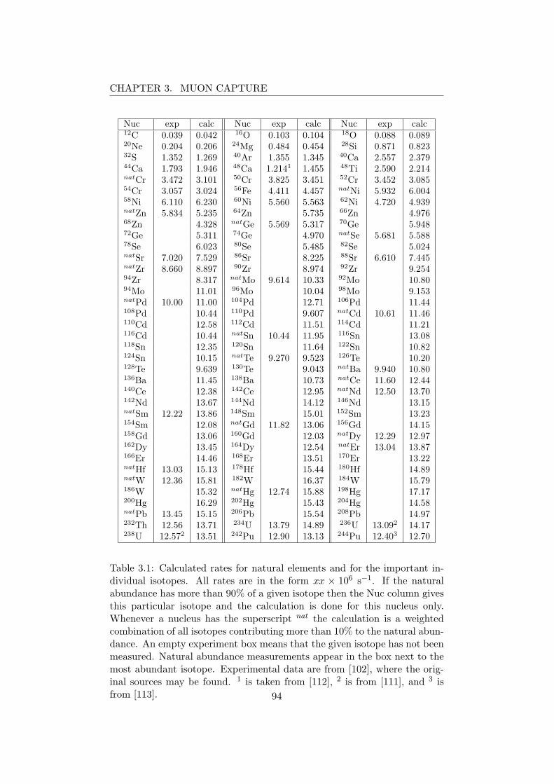
CHAPTER 3. MUON CAPTURE
Nuc exp calc Nuc exp calc Nuc exp calc12C 0.039 0.042 16O 0.103 0.104 18O 0.088 0.08920Ne 0.204 0.206 24Mg 0.484 0.454 28Si 0.871 0.82332S 1.352 1.269 40Ar 1.355 1.345 40Ca 2.557 2.37944Ca 1.793 1.946 48Ca 1.2141 1.455 48Ti 2.590 2.214natCr 3.472 3.101 50Cr 3.825 3.451 52Cr 3.452 3.08554Cr 3.057 3.024 56Fe 4.411 4.457 natNi 5.932 6.00458Ni 6.110 6.230 60Ni 5.560 5.563 62Ni 4.720 4.939natZn 5.834 5.235 64Zn 5.735 66Zn 4.97668Zn 4.328 natGe 5.569 5.317 70Ge 5.94872Ge 5.311 74Ge 4.970 natSe 5.681 5.58878Se 6.023 80Se 5.485 82Se 5.024natSr 7.020 7.529 86Sr 8.225 88Sr 6.610 7.445natZr 8.660 8.897 90Zr 8.974 92Zr 9.25494Zr 8.317 natMo 9.614 10.33 92Mo 10.8094Mo 11.01 96Mo 10.04 98Mo 9.153natPd 10.00 11.00 104Pd 12.71 106Pd 11.44108Pd 10.44 110Pd 9.607 natCd 10.61 11.46110Cd 12.58 112Cd 11.51 114Cd 11.21116Cd 10.44 natSn 10.44 11.95 116Sn 13.08118Sn 12.35 120Sn 11.64 122Sn 10.82124Sn 10.15 natTe 9.270 9.523 126Te 10.20128Te 9.639 130Te 9.043 natBa 9.940 10.80136Ba 11.45 138Ba 10.73 natCe 11.60 12.44140Ce 12.38 142Ce 12.95 natNd 12.50 13.70142Nd 13.67 144Nd 14.12 146Nd 13.15natSm 12.22 13.86 148Sm 15.01 152Sm 13.23154Sm 12.08 natGd 11.82 13.06 156Gd 14.15158Gd 13.06 160Gd 12.03 natDy 12.29 12.97162Dy 13.45 164Dy 12.54 natEr 13.04 13.87166Er 14.46 168Er 13.51 170Er 13.22natHf 13.03 15.13 178Hf 15.44 180Hf 14.89natW 12.36 15.81 182W 16.37 184W 15.79186W 15.32 natHg 12.74 15.88 198Hg 17.17200Hg 16.29 202Hg 15.43 204Hg 14.58natPb 13.45 15.15 206Pb 15.54 208Pb 14.97232Th 12.56 13.71 234U 13.79 14.89 236U 13.092 14.17238U 12.572 13.51 242Pu 12.90 13.13 244Pu 12.403 12.70
Table 3.1: Calculated rates for natural elements and for the important in-dividual isotopes. All rates are in the form xx × 106 s−1. If the naturalabundance has more than 90% of a given isotope then the Nuc column givesthis particular isotope and the calculation is done for this nucleus only.Whenever a nucleus has the superscript nat the calculation is a weightedcombination of all isotopes contributing more than 10% to the natural abun-dance. An empty experiment box means that the given isotope has not beenmeasured. Natural abundance measurements appear in the box next to themost abundant isotope. Experimental data are from [102], where the orig-inal sources may be found. 1 is taken from [112], 2 is from [111], and 3 isfrom [113]. 94
Chapter 4
Neutrinos and Proton-RichEjecta
4.1 Introduction
In nature one finds small abundances of proton-rich (p) nuclei. 1 They aregenerally believed to be produced by a photo dissociation process (called thep-process) and the conditions for such reactions to take place and producethe right abundances was already discussed in the classical nucleosynthesiswork of B2FH [6] and Cameron [7]. The site of this process is thought tobe the hot Supernova environment. However, while heavy p nuclei are ac-counted for by photo disintegration of preexisting heavy elements (producedin neutron capture processes), the lighter ones are under produced in pre-vious studies [115, 116, 117]. The p-process has therefore been shrouded bymystery throughout the 50 years that have elapsed since the foundationalwork of B2FH.
There is strong evidence from galactic chemical evolution studies thatlight elements are produced in primary processes [118, 119, 120]. This meansthat the environment must simultaneously produce the seed nuclei on whichto capture neutrons or protons. This is true for the r-process, whereas thes-process that produces the heavy nuclei around stability is secondary. Forp nuclei the mechanism is largely unknown but there are indications thatsuggest primary Supernova birth for these as well [121]. The same indicationcomes about from measurements of hyper-metal-poor stars in the Milky Way[122] (as discussed in chapter (1)).
Meanwhile, a number of recent Supernova simulation studies have foundthat the ejected matter from the innermost regions around the mass cutis proton-rich during the early stage of the explosion [123, 124, 125]. Theproton densities and temperatures in this matter are in line with the sug-gestions of B2FH and it therefore seems a viable candidate for p-process
1These nuclei lie above the line of β-stability in the nuclear chart.
95

CHAPTER 4. NEUTRINOS AND PROTON-RICH EJECTA
nucleosynthesis. As we will discuss below, neutrinos have a decisive influ-ence on both the proton-richness and the subsequent nucleosynthesis of theinnermost supernova ejecta. This is not surprising since the material sitsclose to the protoneutron star and the flux of neutrinos is large. Our mainconcern is the influence of these neutrinos on the composition of these innerlayers of matter. As we will see, this environment holds promise toward aconsistent production of light p nuclei in a collaborative effort of neutrinosand protons that we have termed ’the νp-process’.
4.2 Neutrino Reactions on Matter
As mentioned, the innermost ejecta that we want to study are subject tolarge neutrino fluxes. We thus need to consider their effect on the mate-rial. The important quantity of concern to us is the electron fraction Ye
introduced in chapter (1). It is determined by the interplay of the weakinteractions in the material, mainly through the reactions
νe + n p+ e− (4.1)νe + p n+ e+. (4.2)
We thus see that dominant neutrino/positron capture can drive the mate-rial proton-rich, whereas neutrino emission and electron capture will drive itneutron-rich. The balance between these reactions can be quite complicatedin realistic models and the subsequent evolution equations must be solvednumerically for the relevant environment given by the hydrodynamical stel-lar model. We will briefly touch upon this in the next section.
It is worth discussing a few aspects of the physics governing Ye and par-ticularly the conditions for proton-richness of the material (this is discussedin some detail in [129], building on the classic study by Bruenn [130]). Therelevant variables are the electron chemical potential µe, the neutron-protonmass difference Mnp = 1.293 MeV, and the neutrino energy. In dense en-vironments, the electron gas is squeezed to degeneracy with large µe andfavorable conditions for electron capture on nucleons and nuclei. However,as the star explodes, matter is diluted and µe drops. The neutrino andantineutrino energies dominate over both µe and Mpn and under these con-ditions the evolution of Ye is given by [131]
dYe
dt≈ λνen − Ye(λνen + λνep), (4.3)
where the λ’s are the rates for the processes in subscript. In weak equilibriumwe have
dYe
dt= 0⇒ (Ye)eq =
λνen
λνen + λνep. (4.4)
96

CHAPTER 4. NEUTRINOS AND PROTON-RICH EJECTA
This ratio can be expressed in terms of the average neutrino energies, lu-minosities and Mpn as given by eq. (77) of [131]. Under the assumptionof similar neutrino and antineutrino luminosities, one can proceed to showthat the material will be proton-rich in weak equilibrium when the followinginequality is satisfied [129]
4Mpn > (〈Eνe〉 − 〈Eνe〉) , (4.5)
where the energies on the right-hand side are the averages over the neutrinospectra.
This inequality is thus the indicator as to when the material will beproton-rich. However, we note that these are all equilibrium considerationsand the ejecta will generally not reach this state before the weak reactionsthat determine Ye freeze out. The true value of Ye will evolve toward theequilibrium value given above for the local conditions of the matter (den-sity, temperature, reaction timescale etc.). The full simulation results givenin [129] show that this evolution toward equilibrium will yield proton-richmatter for the innermost layers, yielding a good candidate site for p-processnucleosynthesis.
4.3 Hydrodynamical Simulation
The hydrodynamical calculations that have been performed are based onspherically symmetric simulations with neutrino Boltzmann transport thatinclude effects of general relativity. The details are technical and we referthe reader to [129] and the relevant references therein. The progenitor starmodel had a main sequence mass of 20 M [132]. However, as we have al-ready discussed in section (1.3), this sort of core-collapse simulation does notproduce explosions. We therefore have to introduce some artificial mecha-nism to force a successful explosion and subsequent ejection of the stellarenvelope.
The expected sensitivity of the matter composition in the innermostejecta to the actual explosion mechanism is a major concern. Previously,people have employed artificial thermal bombs (raising the temperature at agiven radius) or pistons (pushing the matter layers) to explode the models.The observational knowledge of the total explosion energy gives us a handleon the input needed and such techniques have been used to model the outerlayers. These methods will not give the mass cut consistently from thesimulation and this must be determined from other conditions. Clearly,these kinds of forced explosions are not good for innermost ejecta.
The technique used to explode the models here is scaling. The first(model A) method multiplies the neutral current neutrino scattering crosssections by a factor between 0.1 and 0.7. This will decrease the neutrinoopacity in the protoneutron star and thus allow more diffusion out of the
97

CHAPTER 4. NEUTRINOS AND PROTON-RICH EJECTA
Figure 4.1: Time evolution after core bounce of an ejected layer at 0.005 Moutside of the mass cut from a 20 M supernova progenitor. Top left: Luminosity ofneutrinos and antineutrinos. Bottom right: Electron fraction Ye. Top left: Averageneutrino and antineutrino energies εν = 〈E2
ν〉/〈Eν〉 (thick solid and dashed lines).The difference in average neutrino energy, (εν−εν) (thick dot-dashed line) and fourtimes the mass difference between neutron and protons (thin dashed line) are shownin the lower part. Bottom right: Individual weak interaction contributions leadingto Ye > 0.5. The individual contributions from neutrino/antineutrino captures andelectron/positron captures are a factor ten larger than the total resulting dYe/dt.Adapted from [129].
high density region. This will in turn boost the luminosity in the heatingregion (where the material receives the needed kinetic energy to escape thegravitational field). This is expected to represent effects of convection inthe protoneutron star region below. The second method (model B) puts ascaling factor larger than one on the rates for the reactions given in eqs.(4.1) and (4.2) in the heating region. This reduces the neutrino heatingtimescale and is done to mimic possible convective overturn in these highlyunstable layers.
The important point about both methods above is that they will notinfluence the equilibrium temperature and Ye. For model A this is trivialsince nothing is changed in the heating region expect the neutrino luminosi-ties, whereas for model B we have an equal factor on all weak reactions thatchange Ye. We therefore expect the value of Ye to reflect the results of amore involved multi-D model producing explosions. Another nice feature ofthese artificial explosion mechanisms is the fact that the mass cut emerges
98
CHAPTER 4. NEUTRINOS AND PROTON-RICH EJECTA
from the model automatically and we do not need any external conditionsto determine where the innermost ejecta are located.
In figure (4.1) we show the time evolution of various quantities that wehave discussed above as a function of time after core bounce. The figurecorresponds to a layer that is 0.005 M outside the mass cut. The initialpeak seen in the neutrino luminosity just after bounce comes from electroncaptures on the protons that the shock produces by dissolving nuclei (be-fore the shock arrives, the protons are inside neutron-rich nuclei with largeelectron capture thresholds that suppress this reaction). The initial Ye ofthe layer is a result of the progenitor model which has mainly iron groupnuclei in these regions (see the bottom left in figure (4.1)). The neutrons inthese nuclei are protected from the n+ νe reaction relative to free nucleonsso there is little effect from the initial luminosities (antineutrino capturesare suppressed by nuclear structure Pauli blocking effects). Ye is thereforeset by these iron group nuclei which have a value slightly below 1/2.
The shock front passes the mass zone just after 0.2 s, dissociating thenuclei and lowering the density. The small bumps in Ye just after the shockare a result of the complicated interplay of the reactions in eqs. (4.1) and(4.2) as a function of density and temperature. However, ultimately thedecrease of the chemical potential µe leads to more neutrino absorption thanemission, thus driving Ye above 1/2. In the top right portion of figure (4.1)the neutrino and antineutrino energies are shown and compared to 4Mpn
which was the indicator of proton-richness introduced above. We clearly seethat the energy difference (thick dot-dashed line) is always below 4Mpm.
The proton-rich innermost ejecta are found for models A and B [129].However, the extend of this Ye > 1/2 region (and the location of the masscut itself) varies with the values of the rate reduction/enhancement factors.When considering regions from the mass cut and out to 0.1 M the averageYe is still close to the progenitor value. The strong convective instability ofthe region does make it likely that mixing will occur on a short timescaleand we expect Ye to remain high on average (this is also discussed in [133]).
4.4 Network and Neutrinos
The effect of neutrinos on nucleosynthesis of light and medium mass ele-ments in the supernova mantle was first introduced in [126, 127] and con-sidered in great detail by Woosley et al. [128]. Since then a great number ofstudies have considered the effects of neutrinos on various nucleosynthesisprocesses. The core-collapse environment that we are concerned with is oneof primary production of light and medium mass elements and we there-fore need to consider a great number of nuclei in our network and all theirrelevant interactions.
As discussed in [129], the nucleosynthesis of the material was calculated
99
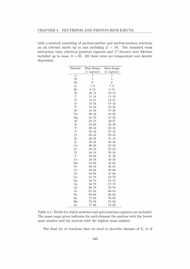
CHAPTER 4. NEUTRINOS AND PROTON-RICH EJECTA
with a network consisting of nucleus-nucleus and nucleus-nucleon reactionson all relevant nuclei up to and including Z = 50. The standard weakinteraction rates (electron/positron captures and β±-decays) were likewiseincluded up to mass A = 65. All these rates are temperature and densitydependent.
Element Mass Range Mass Range(ν capture) (ν capture)
n 1 1H 1 1He 6 6Li 7–9 7–9Be 8–12 8–12B 10–14 10–14C 11–18 11–18N 13–21 13–21O 14–22 14–22F 16–26 16–26Ne 18–29 17–29Na 20–32 19–22Mg 21–35 21–35Al 22–37 22-37Si 24–39 23–39P 26–42 25–42S 28–42 27–42Cl 30–42 29–42Ar 32–44 31–44K 34–48 33–48Ca 36–50 35–50Sc 38–52 37–52Ti 40–54 39–54V 42–56 41–56Cr 44–58 43–58Mn 45–62 45–62Fe 48–64 46–64Co 50–66 49–66Ni 52–68 51–68Cu 54–70 53–70Zn 56–74 55–74Ga 58–78 57–78Ge 60–78 59–78Se 67–84 66–84Br 69–86 68–86Kr 71–92 70–92Rb 73–92 72–92Sr 77–80 74–80
Table 4.1: Nuclei for which neutrino and anti-neutrino captures are included.The mass range given indicates for each element the nucleus with the lowestmass number and the nucleus with the highest mass number.
The final set of reactions that we need to describe changes of Ye is of
100
CHAPTER 4. NEUTRINOS AND PROTON-RICH EJECTA
course neutrino and antineutrino captures. In table (4.1) we give all nucleifor which these rates were included in the network. These range from Hy-drogen and neutrons up to 120Sn. The range of masses chosen for each Z isfrom the proton drip line to stability, including also a few mass units towardthe neutron drip line. Since we are concerned with proton-rich matter thisseems a sensible choice.
The neutrino and antineutrino capture cross sections were calculated forseveral values of the neutrino spectral temperature between 2.8 and 10 MeV.Through eq. (2.83), this converts into average neutrino energies between 8.8and 31.5 MeV. By using interpolation between these values we describe thecross sections consistently for all relevant average energies. We can thus usethe detailed neutrino energy information under the assumption of a Fermi-Dirac spectrum.
We should mention that neutrino scattering events were not includedsince they do not change Ye. They can, however, change composition byspallation events during deexcitation. This will be implemented in futurework.
4.5 νp-process Nucleosynthesis
The nucleosynthesis was followed with all the reactions mentioned aboveincluded for the inner, proton-rich layers (defined by the condition Ye > 1/2)where we expect free protons to exist. This layer had different thickness formodels A and B, and for the different parameters. However, the abundanceyields turn out very similar (see [129]). We therefore focus on the modelB07 as in [134] (referring to a factor of 7 on the rates of the reactions in eqs.(4.1) and (4.2)).
In figure (4.2) we show the abundance evolution as a function of timeafter bounce. The solid lines are with neutrino interactions in the network,whereas the dashed ones are without. We clearly see a large effect on Ye andthe neutron abundance. The curve for 56Ni is an indicator as to the timewhen nuclei start to form. We note that the inclusion of neutrino reactionson nuclei has practically no effect on Ye.
The enhanced potential for nucleosynthesis of this environment comesfrom the increased neutron abundance produced by antineutrino captures onthe proton-rich material. Capture on protons and nuclei occur on timescalesthat are short (a few seconds) at the nuclear production radius of roughly1000 km (much shorter than the β-decay lifetimes of nuclei like 56Ni and64Ge). For neutrinos this is a different story since there is a threshold forcapture on the proton-rich side of stability. The larger abundance of protonsin the material thus leads us to a situation where antineutrino captures onprotons produce a significant abundance of free neutrons. These neutronsdo not suffer from small binding energies that would otherwise inhibit the
101

CHAPTER 4. NEUTRINOS AND PROTON-RICH EJECTA
Figure 4.2: Evolution of the abundance of neutrons, protons, α-particles, and 56Niin a nucleosynthesis trajectory resulting from model B07 of reference [129]. Theabundance, Y , is defined as the number of nuclei of the species i present divided bythe total number of nucleons which is conserved during the calculation. The solid(dashed) lines display the nucleosynthesis results which include (omit) neutrino andantineutrino absorption interactions after nuclei are formed. The abscissa measuresthe time since the onset of the supernova explosion.
nucleosynthesis process.The abundances that we get from the calculation are shown as filled
circles in figure (4.3). The open circles show the same calculation with noneutrinos included for comparison. The results are given relative to solarabundances. We immediately see a striking difference for A > 64 when weinclude the neutrinos. This feature has been traced to a novel mechanismthat allows one to overcome waiting points that arise due to β lifetimesand Coulomb barriers. The abundances for the heavier nuclei are up to 105
times larger than the solar values in figure (4.3). This is compensated by thesmall amount of material with Ye > 1/2 in the model. Since this amount isaround 10−5 M the solar abundances can be produced if all the proton-richmaterial is ejected by the explosion.
The synthesis of elements with A > 64 was obtained in proton-rich ejectain previous studies also [136]. However, those studies required entropies perbaryon of s ≈ 150 − 170 kB which is roughly a factor of three above theestimates for core-collapse events [133, 129]. 2 The scenario presented here
2The entropy variable can seem counterintuitive when discussing nucleosynthesis. Someclarifications of this issue can be found in appendix (C).
102

CHAPTER 4. NEUTRINOS AND PROTON-RICH EJECTA
0 10 20 30 40 50 60 70 80 90 100Mass Number A
10−3
10−2
10−1
100
101
102
103
104
105
106
107Y
i/Yi,⊙
With νWithout ν
Figure 4.3: Abundances for model B07 relative to solar abundances [135]. Twodifferent calculations are shown: with neutrino-induced reactions in the network(filled circles) and without neutrino-induced reactions in the network (open circles).
is therefore much more realistic and in fact expected to be generic as we willdiscuss at the end of this chapter.
The key waiting point that one has to get across in order to get apprecia-ble nucleosynthesis ofA > 64 nuclei is 64Ge. The (p, γ) reaction is suppressedby the negative proton seperation energy of 65As. Furthermore, 64Ge has aβ lifetime of about 64 s, much longer than the expansion timescale of order10 s so β-decay will also be too slow. In the presence of free neutrons onecan, however, bypass this by the (n, p) reaction which has a lifetime of about0.25 s at the relevant temperature (2 · 109 K), shorter than the dynamicaltimescale. One can therefore produce 64Ga which can capture further pro-tons. This allows the flow to continue until the next α nucleus, 68Se, andthen the story repeats. 3 This novel process has been dubbed the νp process[134]. As one can see in figure (4.3) the flow of matter stops just belowA = 100. Here one reaches the region of 100Sn where α-decay ends the flow(analogous to the cycle at 210Po in the s-process discussed in chapter (1)).A similar flow termination cycle was found around 106−108Te by Schatz etal. [137] for the rp-process.
3One would perhaps also expect neutrinos and antineutrino captures to play a role inbreaching these waiting points. Simple estimates show, however, that the lifetime againstcapture for nuclei like 64Ge is of the order of several seconds. Thus the (n, p) reaction willstill be dominant.
103
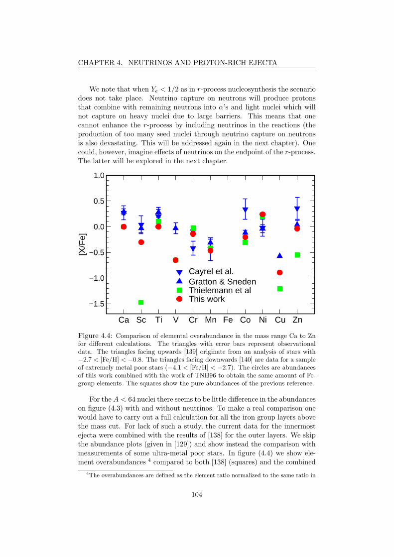
CHAPTER 4. NEUTRINOS AND PROTON-RICH EJECTA
We note that when Ye < 1/2 as in r-process nucleosynthesis the scenariodoes not take place. Neutrino capture on neutrons will produce protonsthat combine with remaining neutrons into α’s and light nuclei which willnot capture on heavy nuclei due to large barriers. This means that onecannot enhance the r-process by including neutrinos in the reactions (theproduction of too many seed nuclei through neutrino capture on neutronsis also devastating. This will be addressed again in the next chapter). Onecould, however, imagine effects of neutrinos on the endpoint of the r-process.The latter will be explored in the next chapter.
Ca Sc Ti V Cr Mn Fe Co Ni Cu Zn
−1.5
−1.0
−0.5
0.0
0.5
1.0
[X/F
e]
Cayrel et al.Gratton & SnedenThielemann et al This work
Figure 4.4: Comparison of elemental overabundance in the mass range Ca to Znfor different calculations. The triangles with error bars represent observationaldata. The triangles facing upwards [139] originate from an analysis of stars with−2.7 < [Fe/H] < −0.8. The triangles facing downwards [140] are data for a sampleof extremely metal poor stars (−4.1 < [Fe/H] < −2.7). The circles are abundancesof this work combined with the work of TNH96 to obtain the same amount of Fe-group elements. The squares show the pure abundances of the previous reference.
For the A < 64 nuclei there seems to be little difference in the abundanceson figure (4.3) with and without neutrinos. To make a real comparison onewould have to carry out a full calculation for all the iron group layers abovethe mass cut. For lack of such a study, the current data for the innermostejecta were combined with the results of [138] for the outer layers. We skipthe abundance plots (given in [129]) and show instead the comparison withmeasurements of some ultra-metal poor stars. In figure (4.4) we show ele-ment overabundances 4 compared to both [138] (squares) and the combined
4The overabundances are defined as the element ratio normalized to the same ratio in
104
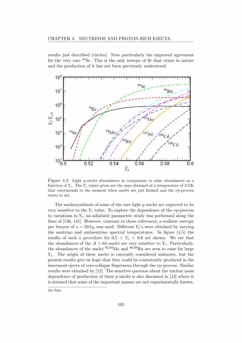
CHAPTER 4. NEUTRINOS AND PROTON-RICH EJECTA
results just described (circles). Note particularly the improved agreementfor the very rare 45Sc. This is the only isotope of Sc that exists in natureand the production of it has not been previously understood.
Figure 4.5: Light p-nuclei abundances in comparison to solar abundances as afunction of Ye. The Ye values given are the ones obtained at a temperature of 3 GKthat corresponds to the moment when nuclei are just formed and the νp-processstarts to act.
The nucleosynthesis of some of the rare light p nuclei are expected to bevery sensitive to the Ye value. To explore the dependence of the νp-processto variations in Ye, an adiabatic parametric study was performed along thelines of [136, 141]. However, contrary to those references, a realistic entropyper baryon of s = 50 kB was used. Different Ye’s were obtained by varyingthe neutrino and antineutrino spectral temperatures. In figure (4.5) theresults of such a procedure for 0.5 < Ye < 0.6 are shown. We see thatthe abundances of the A > 64 nuclei are very sensitive to Ye. Particularly,the abundances of the nuclei 92,94Mo and 96,98Ru are seen to raise for largeYe. The origin of these nuclei is currently considered unknown, but thepresent results give us hope that they could be consistently produced in theinnermost ejecta of core-collapse Supernova through the νp process. Similarresults were obtained by [12]. The sensitive question about the nuclear massdependence of production of these p nuclei is also discussed in [12] where itis stressed that some of the important masses are not experimentally known.
the Sun.
105
CHAPTER 4. NEUTRINOS AND PROTON-RICH EJECTA
In closing we summarize the facts that lead us to believe that the νp-process described here is actually a generic feature of Type II Supernova.Recent core-collapse models that start from different progenitor models andemploy 1D and 2D simulations of transport all indicate that proton-richnessis a feature of the innermost ejecta [123, 124, 125, 133, 129]. There is alsolittle doubt that these layers will be subject to intense neutrino fluxes fromthe protoneutron star region below. This latter fact has already promptedstudies in the past that found evidence for p nuclei production in such in-tense neutrino fluxes [47, 142]. One could still worry about whether fallbackcould prevent the nuclei from getting out into the interstellar medium but,as discussed in [143], mixing before fallback will always lead to some ejec-tion also for the innermost layers. We therefore believe that the process willoperate in all core-collapse Supernova. The sensitivity to the actual explo-sion mechanism could mean that the yields will be very dependent on stellarmass, rotation, magnetic fields etc. This is not a bad thing, since it mighthelp to explain diversities found in observations of enriched stars. It willbe interesting to see the process operating in a nucleosynthesis calculationof the full ejecta and likewise to see how it will influence galactic chemicalevolution studies.
106

Chapter 5
Neutrinos and the r-process
5.1 r-process Nucleosynthesis
The synthesis of heavy elements in the r-process and the nuclear reactionsthat are involved in this process will be our main focus for the remainderof the thesis. We therefore provide a brief overview of some central fea-tures needed for this discussion. As was mentioned in the introduction,the r-process produces elements through neutron captures on a timescalemuch faster than the β-decay lifetime of the extremely neutron-rich nucleiinvolved. We thus need an astrophysical environment with extreme neutronfluxes. The site for the r-process is not easy to point out and there is notyet full consensus on this issue. However, there is a site connected to core-collapse Supernovae that has been favored by many authors for a number ofyears, and it will be our reference scenario. We will discuss it in more detailbelow, but first we briefly summarize some general features of the r-process.
5.1.1 General Conditions
The r-process is responsible for producing about half of the elements heav-ier than iron that we find in the solar system, and it is (presumably) thesole production event for nuclei heavier than 209Bi. The classical processis assumed to take place in an equilibrium between the (n, γ) and (γ, n)reactions, both of which are assumed much faster than β-decays. The Sahaequation for the equilibrium abundances now gives us a relation for the ratioof abundances
Y (Z,A+ 1)Y (Z,A)
∝ ρn exp(Sn(Z,A+ 1)
T
), (5.1)
where ρn is the neutron number density and T is the temperature of thematerial. The process therefore occurs in nuclei that have the same neutronseparation energy Sn, the value of which is typically 2-3 MeV (depending
107

CHAPTER 5. NEUTRINOS AND THE R-PROCESS
on the neutron density and the temperature). Assuming a steady flow, wealso have β equilibrium
λβ(Z − 1)Y (Z − 1) = λβ(Z)Y (Z), (5.2)
where Y (Z) =∑
A Y (Z,A) is the total yield of a particular element andλβ(Z) =
∑A λβ(Z,A)Y (Z,A)/Y (Z) is the β-weighted abundances. We
thus see that the total yields are inversely proportional to the total rates, orproportional to the lifetime. For given Z there is usually one or two nucleithat have the Sn to be on the r-process path. These are the waiting pointnuclei, since the process has to wait for their β-decay to proceed furtherup the nuclear chart. This, in turn, means that nuclei with magic numbershave high yields due to the small Sn and long β lifetimes (these peaks canbe clearly seen in figure (1.3)).
The discussion above shows us that two key ingredients needed to modelthe process are ρn and T . Through various constraints (including the veryimportant fact that the process needs to reproduce the solar abundanceswhen s-process elements are subtracted) one finds that neutron densities of1022− 1024 cm−3 and temperatures of about 109 K (∼ 100 keV) are needed.Considering that the actinides have to be produced, we can estimate theduration of the process by summing all the β lifetimes of the waiting pointnuclei up to mass A ∼ 240. This tells us that the r-process lasts for about1-2 s. This way of viewing the process is called classical r-process. Later wewill be concerned with presumably more realistic dynamical models wherethe conditions change with time. The process eventually stops at the veryheavy nuclei since the fission channel opens up. We will have more to sayabout this end-point issue in the next chapter.
The process terminates when ρn drops significantly below the valuesgiven above, referred to as the freeze-out. In stellar ejecta the point andtime at which this happens is determined by the outflow velocity (throughthe radial dependence of the neutron flux). After freeze-out one needs tofollow the nuclei as they β-decay back to stability and give the final nucle-osynthesis results. During this period there can still be neutrons releasedthat induce further fission reactions. This will also be addressed in thesubsequent chapter.
The density, temperature, and duration given above indicate that explo-sive conditions are required. The observations of metal-poor star indicatethat the process is likely primary and we therefore have good reason tobelieve that it could be connected to core-collapse Supernovae.
5.1.2 The Neutrino-driven Wind
As mentioned, the site of the r-process is still not fully agreed upon. Anearly suggestion was the He-shell which is also the site of the s-process. Thiscould, however, not produce the neutron fluxes needed. Later suggestions
108
CHAPTER 5. NEUTRINOS AND THE R-PROCESS
include neutron-star mergers, Supernova fallback, magnetic winds and ac-cretion disks. The currently favored site is a neutrino-driven wind that isthought to occur above the mass cut of core-collapse Supernovae. This lat-ter scenario is the one that we will assume and we therefore proceed to givefurther details of this environment.
Some of the first papers to emphasize the potential for r-process nucle-osynthesis in the hot neutrino-driven wind above the protoneutron star werethose of Woosley and Hoffmann [144] and Meyer et al. [145]. The region liesjust behind the stalled shock front from the core bounce and is exposed tohuge neutrino fluxes that come from cooling of the accreting protoneutronstar below. This raises the temperature and the entropy of the material ina low density region called the ’hot bubble’. The entropy typically goes upto several hundreds per baryon and the temperature is around 1010 K. Thishot bubble scenario occurs about 1-20 s after the bounce, so later than theνp-process of the previous chapter.
In figure (5.1) we show a schematic cartoon of the process to help guidethe discussion. The high temperature means that charged particle reactionscan build up nuclei (through the so-called α-process) that can act as seedsfor the free neutrons to capture on. For this process to reach the actinideswe need a neutron-to-seed ratio of roughly 100 (assuming that the chargedparticle reactions will build seed up to A ∼ 100). This would require n/p ∼7− 8 (Ye ∼ 0.1) under normal circumstances. However, the extremely highentropy that one finds in the hot bubble can allow a high neutron-to-seedratio even in moderately neutron-rich material with Ye > 0.4 (see appendix(C)).
The moderate neutron-richness of the material can be produced in core-collapse supernova since (as we have already seen in the model discussed inthe previous chapter) the antineutrino energy is generally higher than theneutrino energy. During the cooling phase one expects equal luminositiesin all species and this will tend to drive the material to Ye < 1/2. There isa danger with the neutrinos since they can capture on neutrons to produceprotons that recombine into αs and thus lower the neutron-to-seed ratio[47]. This can can be avoided by a very fast expansion as discussed in [146].Another very attractive feature of this particular site is that it providesroughly 10−4M per core-collapse Supernova event. This is the right amountwhen one considers the event rate in our galaxy, the total amount of observedmaterial coming from r-process, and the galaxy lifetime and mass [144, 145].
In our discussion of the neutrino-driven wind it should be clear thatone needs rather specialized conditions to make the r-process work in thisenvironment. This is of course the reason for the continued uncertaintyabout the site that still exists (see for example the recent review in [9]).In the r-process studies, that we will present in the next chapter, questionsrelated to site are put aside by simply parameterizing the conditions of thenuclear material that undergoes nucleosynthesis (we will give more detail
109
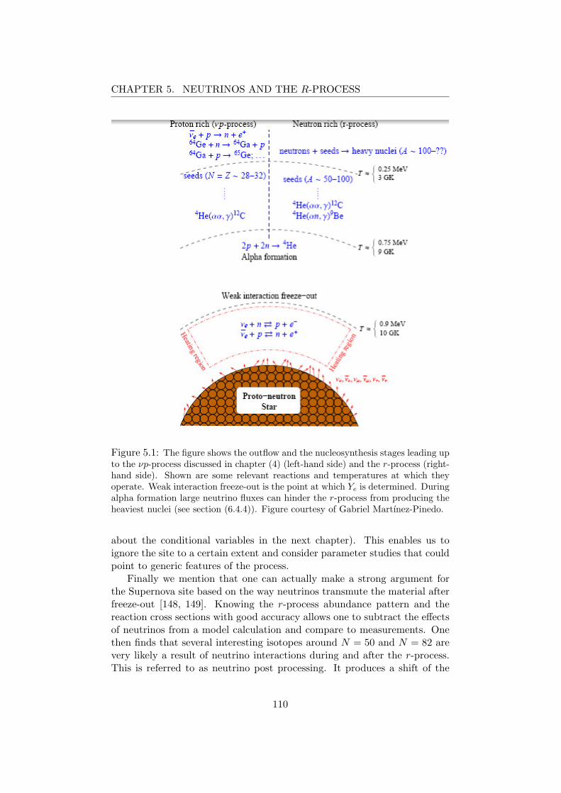
CHAPTER 5. NEUTRINOS AND THE R-PROCESS
Figure 5.1: The figure shows the outflow and the nucleosynthesis stages leading upto the νp-process discussed in chapter (4) (left-hand side) and the r-process (right-hand side). Shown are some relevant reactions and temperatures at which theyoperate. Weak interaction freeze-out is the point at which Ye is determined. Duringalpha formation large neutrino fluxes can hinder the r-process from producing theheaviest nuclei (see section (6.4.4)). Figure courtesy of Gabriel Martınez-Pinedo.
about the conditional variables in the next chapter). This enables us toignore the site to a certain extent and consider parameter studies that couldpoint to generic features of the process.
Finally we mention that one can actually make a strong argument forthe Supernova site based on the way neutrinos transmute the material afterfreeze-out [148, 149]. Knowing the r-process abundance pattern and thereaction cross sections with good accuracy allows one to subtract the effectsof neutrinos from a model calculation and compare to measurements. Onethen finds that several interesting isotopes around N = 50 and N = 82 arevery likely a result of neutrino interactions during and after the r-process.This is referred to as neutrino post processing. It produces a shift of the
110

CHAPTER 5. NEUTRINOS AND THE R-PROCESS
abundance peaks to the left since the reactions spallate neutrons from thesynthesized nuclei. During the r-process there will also be an effect on thewaiting points since neutrino capture can aid β-decays in bridging these andmove the matter flow upward (still allowing for the observed peaks aroundmagic numbers). These neutrino effects can therefore be used to constrainthe neutrino flux, dynamical time scale, and freeze-out radii. In [148, 149]these considerations were found to favor the core-collapse Supernova site.
5.2 UMP Stars and Neutrino-induced Fission
As we have already discussed in chapter (1), recent advances in observationsof elemental abundances in ultra-metal poor (UMP) stars provide us withdetailed information about the heavy nuclei that the r-process is believedto be responsible for. We showed abundance pattern for several UMP starsin figure (1.4) and pointed out the astonishing agreement with solar values.In figure (5.2) we show the UMP star CS 22892-052 pattern in more detail,including the measurement of lighter nuclei with Z < 50 (or A < 130). Theagreement with the scaled solar abundances (solid line) is seen to be worse,particularly for the nuclei Rh, Pd, Ag, and Cd. One is therefore promptedto study how the r-process scenario described above can accommodate suchvariations.
In early studies of fission dynamics in the r-process it has been found thatfission cycling can occur [152]. This means that matter that undergoes fissionduring the process produces fragments that continue to capture neutrons andmove upwards along the flow. Under certain conditions this can effectivelycreate a cycle for the involved nuclei. This effect was seen in several studies[153, 154], and in particular one found a robust abundance pattern for A >130 [155]. Naively, the regular abundance pattern found for A > 130 in UMPstars can now be explained by an r-process with a neutron-to-seed ratio largeenough for fission cycling and the lower mass elements could be attributedto an appropriately smaller neutron-to-seed ratio (or an incredibly effectives-process component in early generation stars) [156]. But, as shown byQian [156, 9], the assumption of a robust cycling producing A > 130 nucleicontradicts observations in the UMP stars CS 31082-001. So it seems thatanother mechanism must be operating.
This led Qian [156] to suggest that, assuming the nucleosynthesis tookplace in an environment of intense neutrino fluxes, a process with fissionbut no fission cycling could explain the observations. The proposal usesneutrino reactions as a way of getting the progenitor r-process nuclei tofission after freeze-out. Qian’s scenario starts from a freeze-out distributioncovering 190 < A < 320 so a large neutron-to-seed ratio would be needed butwithout fission cycling. Recent fission barrier calculations for neutron-richnuclei that are generally higher than previous calculations seem to support
111

CHAPTER 5. NEUTRINOS AND THE R-PROCESS
Figure 5.2: Measured abundances of neutron capture elements in CS 22892-052(filled circles; data from [150]) compared to solar r-process pattern (solid line),translated to fit the Eu data. Solar pattern is obtained by subtraction of model-based s-process from the solar values [151].
the absence of cycling due to a pile up of matter at high mass [72] (we willreturn to this point in the next chapter). Spontaneous fission is assumedto occur for all nuclei with 260 < A < 320 and for some of those in therange 230 < A < 260. The highly energetic neutrinos are then supposed tocause an enhancement of fission for 230 < A < 260 and perhaps even for190 < A < 230.
The fragments from the fission events in Qian’s proposal are then sup-posed to fall in the interval 86 < A < 109 with enhanced structures atA ∼ 90 (from fission of the A ∼ 195 peak) and A ∼ 132 (from the fission of230 < A < 320 which will likely have a fragment in the doubly magic 132Snregion). Qian goes on to estimate the ratio of fission yields 86 < A < 190to surviving nuclei in the range 190 < A < 260 under these assumptionsand finds that around 40% of the 190 < A < 260 nuclei must fission toaccommodate the data from CS 22892-052 and about 20% for CS 31082-001. This difference can potentially be explained by varying the amount ofneutrino-induced interactions on the nuclei after freeze-out. The neutrinoflux from cooling is expected to last about 20 s [157] so there is plenty oftime for neutrino reactions after freeze-out (during the r-process neutrino
112

CHAPTER 5. NEUTRINOS AND THE R-PROCESS
captures are severely limited for the A ∼ 195 peak to be produced [47]).The number of neutrino-induced fission events will vary with the neutrinoluminosity and time scale of cooling and differences in these variables couldthen explain the observations. The needed level of neutrino reactions is alsoconsistent with the previously discussed post processing [148, 149].
After the freeze-out the material will start to β-decay back toward thevalue of stability. Therefore the charge will increase and this influencesthe fission probability of a given nucleus. 1 One could therefore hope thatnumerous β-decays will increase the probability for neutrino reactions tocause fission. However, this must happen when the neutrino flux is ap-preciable during the first 20 s after core bounce. Using the β lifetimes of[30], Qian estimates that Z can increase about 8 units within the first 10seconds for 190 < A < 260. So for the above scenario to work one needsneutrino-induced fission to become significant during these eight steps. Wewill return to this when we present our detailed calculations of the neutrinocross sections below.
5.3 Neutrino-induced Fission on r-process Nuclei
The suggestions of Qian described above clearly requires detailed calcula-tions of the neutrino-induced fission reaction both on the r-process path andon the decay back to stability. The first calculations along these lines waspresented recently in Kolbe et al. [158]. That study considered the neutrinocapture cross sections of selected isotopes with Z = 84 − 92 for the fissionand neutron emission channels (the dominant ones for neutron-rich matter).However, [158] used a model where only the first decay of the deexcitationin the daughter was considered, meaning that potential fission events af-ter neutron emission(s) were not taken into account. The neutrinos haveenergies that are high enough for the latter processes to contribute. Thecalculations of [158] were also unable to give information about the fissionyield distributions. These facts made it difficult to evaluate the potential ofQian’s proposal.
The desire to remedy the above situation was part of the motivationthat led to us to develop the nuclear model presented in section (2.4). Thefirst application of it was therefore naturally the calculation of cross sectionsand fragment distributions for charged current neutrino-induced fission onr-process relevant nuclei [159]. Note that this process starts with a neutrinocapture (ν, e−) which means that the decaying daughter nucleus has chargeZparent + 1. The rest of this chapter will be devoted to the discussion ofour results and how they influence the Qian scenario. However, for a fullcomparison one needs to put the nuclear data obtained into a detailed nu-
1From the surface to coulomb term one can estimate that the fission probability scaleswith Z2/A.
113

CHAPTER 5. NEUTRINOS AND THE R-PROCESS
cleosynthesis network calculation. This will be the focus of the next chapterin which we will see the influence of neutrinos on the fission dynamics of ther-process.
5.3.1 Initial Uranium Calculations
The first calculations we did were for neutrino-induced processes on uraniumisotopes from A = 238 to A = 302. In figure (5.3) we show the cross sec-tions as a function of neutrino energy. Shown are the total, partial fission,and partial neutron emission results (the latter defined as events where thenucleus survives fission but might emit one or more neutrons during deexci-tation). Other reaction channels, like proton or α emissions, are negligiblefor virtually all nuclei considered. The range of neutrino energies in figure(5.3) covers the entire interval of interest for the reference spectral temper-ature T = 4 MeV.
Figure 5.3: Total (solid) and partial fission (dotted) and neutron evaporation(dashed) cross sections (in 10−42cm2) for neutrino-induced (νe, e
−) reactions onuranium isotopes as function of neutrino energy.
In the figure we can clearly see a strong increase of the cross sections atneutrino energies of around Eν ∼ 17 MeV. This is due to the IAS and GTresonances which open up at around these energies. Notice that the positionswhere these are located are decreasing slightly with mass number, which ismainly a result of the increasing reaction Q-value. The fission channel isseen to dominate in the first two isotopes for Eν > 20 MeV, whereas for thelarger nuclei it is quite small. The latter is expected since Sn becomes verysmall for the heavier isotopes (see table (5.1)), causing the neutron emissionmode to dominate.
114

CHAPTER 5. NEUTRINOS AND THE R-PROCESS
Aprog Sn σtot σfiss σevap σtot [158] σfiss [158]238 6.15 4.71(+02) 3.53(+02) 1.18(+02) 4.93(+02) 3.46(+02)246 4.83 6.05(+02) 3.33(+02) 2.72(+02) 6.31(+02) 3.32(+02)254 4.51 7.10(+02) 1.50(+02) 5.60(+02) 7.84(+02) 5.73(+02)262 3.81 8.48(+02) 4.85(+01) 8.00(+02) 8.57(+02) 5.35(+02)270 3.10 1.05(+03) 3.19(+01) 1.02(+03) 9.39(+02) 3.27(+02)278 1.77 1.46(+03) 2.90(+01) 1.43(+03)286 1.58 1.64(+03) 2.57(+01) 1.61(+03)294 1.16 1.79(+03) 1.28(+02) 1.66(+03)302 0.57 2.06(+03) 1.85(+02) 1.88(+03)
Table 5.1: Total and partial fission and neutron evaporation cross sections (inunits of 10−42 cm2) for neutrino-induced (νe, e
−) reactions on uranium isotopeswith mass numbers Aprog, adopting a Fermi-Dirac distribution with parametersT = 4 MeV and µ = 0 appropriate for supernova νe neutrinos. The exponents aregiven in parentheses. Sn are from [30]. The last two columns give the total and thepartial fission cross sections, as calculated in [158] using the fission barriers of [74].
The folded cross sections for the uranium isotopes are given in table(5.1). We have used a neutrino temperature of T = 4 MeV and chemicalpotential µ = 0 which are the recommended values for Supernova neutrinosas discussed in section (2.4.3). Here we can clearly see that fission is only adominant decay mode for the first two species as expected from the profilesof figure (5.3). The total cross section is seen to increase with mass numberin an almost linear fashion. This is a result of the strengths of the Fermiand GT transitions which depend on N − Z (section (2.2.2)). We can thussee that our earlier statements about the importance of these contributionswere well-founded.
The results presented here differ from the earlier study in [158] wherefission dominated below A = 270 as one can see in the last two columnsof table (5.1). This was expected since those results were obtained withthe barriers of Howard and Moller [74] which are quite low in that regioncompared to the Sierk barriers [71] used here. To investigate this expecta-tion in detail, we did the calculation using the Howard and Moller barriers(with all other ABLA parameters unchanged) and found results similar to[158]. As another test we tried using the recent barriers of Mamdouh et al.[72] which are considerably higher for very neutron-rich nuclei compared toHoward and Moller. The results of this latter test came out roughly thesame as those given above with the Sierk barriers. 2 Earlier investigations[160, 161, 162] have suggested that the larger barriers used here are the morerealistic choice.
2These barrier studies are not self-consistent since only the fission barriers were varied.The masses, shell corrections etc. in the statistical code were not changed accordingly. Assuch we can only rely on this as essentially a barrier parameter study. In the next chapterwe will explore how changes in mass tables, barriers etc. influence the r-process fissiondynamics when done in a more consistent fashion.
115

CHAPTER 5. NEUTRINOS AND THE R-PROCESS
At this point we wish to address the neutrino spectral temperature de-pendence of our results. In table (5.2) we therefore give the total crosssections for neutrino capture reaction on three of the uranium isotopes con-sidered above. Also shown is the percentage of the total cross section thatgoes into the fission channel. The strong increase of the total cross sectionsis of course a result of the increasing average neutrino energy, leading tostronger excitation of the giant resonances and larger phase space factors.The nucleus 278U is on the r-process path (to be discussed below) and onecould therefore be interested in how the lifetime against neutrino capturevaries with T . Using the formula given in appendix (B) we find a lifetimebetween 0.02 s (T = 2.8 MeV) and 0.006 s (T = 10.0 MeV), assuming aluminosity of 1051 erg/s and a radius of 100 km. The estimated β half life is0.018 s [30]. We thus see that neutrinos can compete with β-decays for alltemperatures considered, provided that the reactions occur at this rathersmall radius. However, the dependence on spectral temperature of theseeffects is obvious and must be taken into account in detailed simulations.
Aprog T = 2.8 T = 3.5 T = 4.0 T = 5.0 T = 8.0 T = 10.0
238 1.55(+02) 3.11(+02) 4.71(+02) 8.91(+02) 2.34(+03) 3.00(+03)52 68 75 83 90 91
278 5.62(+02) 1.02(+03) 1.45(+03) 2.52(+03) 5.75(+03) 7.02(+03)1.2 1.7 2.0 2.3 2.7 2.8
302 8.24(+02) 1.46(+03) 2.06(+03) 3.51(+03) 7.83(+03) 9.51(+03)6.3 8.1 9.0 10 11 12
Table 5.2: Total cross section (in units of 10−42 cm2) for neutrino-induced (νe, e−)
reactions on 238U, 278U, and 302U for neutrino spectral temperatures betweenT = 2.8 and T = 10.0 MeV. The exponents are given in parentheses. The fis-sion percentage (σfission/σtot) is given below each cross section.
When looking at the fission percentages in table (5.2) we confirm thediscussion above with regards to the barriers. For 238U fission becomesincreasingly dominant with spectral temperature as the neutrino energy isessentially always above the barrier, whereas for the two heavier isotopes thecontribution from fission is only slightly increasing with T . The latter twohave high barriers and much lower Sn so the behavior is expected. We havealso calculated the average number of neutrons emitted during the reactions.For 238U one gets < N >tot= 1.76 at T = 4 and 2.83 at T = 8 MeV. In278U we found 3.15 and 5.13 and in 302U it is 10.9 and 13.6 (for T = 4 andT = 8 MeV respectively). All numbers given represent the average over bothfission and neutron emission channels. Again the changes with T are notdramatic. However, since the released neutrons can induce further reactionswhen captured on other nuclei one needs to take these effects into account.
The fission fragment yield for the uranium isotopes were also calculatedand in figure (5.4) we show the results for the three selected isotopes of table(5.2). In the figure we give the fragment distributions for neutrino temper-
116

CHAPTER 5. NEUTRINOS AND THE R-PROCESS
Figure 5.4: Mass (top) and charge (bottom) distributions (in percent) of fissionfragments produced in (νe, e
−) reactions on 238U, 278U, and 302U. The black curvesshow the distributions for neutrinos spectral temperature T = 4 MeV and the redcurves show those with T = 8 MeV. Notice that we have varied the range on theyield axis to maximize visibility.
atures T = 4 (black curves) and T = 8 MeV (red curves). In 238U (whosedaughter is 238Np) one sees the double-hump pattern (this is experimentallywell-known in this actinide region [57]). There is a peak around A ∼ 138related to the neutron shell at N = 82 and one at the A ∼ 95. 3 The wriggleson the mass distributions are due to an expected odd-even staggering (seefigure (2.4)). The corresponding charge distributions show peaks at Z = 38and Z = 54 which means that the yields are neutron-rich and will likely un-dergo one or more β-decays toward stability. The heavier isotopes also showthe double-hump structure with 278U showing a clear attraction toward thedoubly-magic region around 132Sn. 302U is a more complicated story, sincewe have to take into account that most fission events are accompanied bymany released neutrons (between 25 and 30 for fission at excitation energiesbelow 10 MeV). The high peak contains slightly more probability since thisis where the symmetric mode lies. The position of the peak (A ∼ 155) isconnected to the presence of a neutron shell closure at N ∼ 88 for deformednuclei (as discussed in section (2.3.2)).
The fragment distributions are thus seen to be quite complicated as afunction of mass number, going from the broad double-hump in 238U, over
3Mass conservation dictates that the sum of fragments and emitted neutrons shouldequal the progenitor mass A. Since we only consider the fission and neutron emissionchannels we therefore have A = Afrag1 + Afrag2 + Nemitted.
117
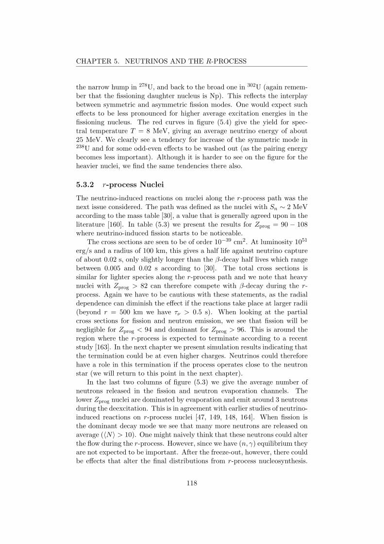
CHAPTER 5. NEUTRINOS AND THE R-PROCESS
the narrow hump in 278U, and back to the broad one in 302U (again remem-ber that the fissioning daughter nucleus is Np). This reflects the interplaybetween symmetric and asymmetric fission modes. One would expect sucheffects to be less pronounced for higher average excitation energies in thefissioning nucleus. The red curves in figure (5.4) give the yield for spec-tral temperature T = 8 MeV, giving an average neutrino energy of about25 MeV. We clearly see a tendency for increase of the symmetric mode in238U and for some odd-even effects to be washed out (as the pairing energybecomes less important). Although it is harder to see on the figure for theheavier nuclei, we find the same tendencies there also.
5.3.2 r-process Nuclei
The neutrino-induced reactions on nuclei along the r-process path was thenext issue considered. The path was defined as the nuclei with Sn ∼ 2 MeVaccording to the mass table [30], a value that is generally agreed upon in theliterature [160]. In table (5.3) we present the results for Zprog = 90 − 108where neutrino-induced fission starts to be noticeable.
The cross sections are seen to be of order 10−39 cm2. At luminosity 1051
erg/s and a radius of 100 km, this gives a half life against neutrino captureof about 0.02 s, only slightly longer than the β-decay half lives which rangebetween 0.005 and 0.02 s according to [30]. The total cross sections issimilar for lighter species along the r-process path and we note that heavynuclei with Zprog > 82 can therefore compete with β-decay during the r-process. Again we have to be cautious with these statements, as the radialdependence can diminish the effect if the reactions take place at larger radii(beyond r = 500 km we have τν > 0.5 s). When looking at the partialcross sections for fission and neutron emission, we see that fission will benegligible for Zprog < 94 and dominant for Zprog > 96. This is around theregion where the r-process is expected to terminate according to a recentstudy [163]. In the next chapter we present simulation results indicating thatthe termination could be at even higher charges. Neutrinos could thereforehave a role in this termination if the process operates close to the neutronstar (we will return to this point in the next chapter).
In the last two columns of figure (5.3) we give the average number ofneutrons released in the fission and neutron evaporation channels. Thelower Zprog nuclei are dominated by evaporation and emit around 3 neutronsduring the deexcitation. This is in agreement with earlier studies of neutrino-induced reactions on r-process nuclei [47, 149, 148, 164]. When fission isthe dominant decay mode we see that many more neutrons are released onaverage (〈N〉 > 10). One might naively think that these neutrons could alterthe flow during the r-process. However, since we have (n, γ) equilibrium theyare not expected to be important. After the freeze-out, however, there couldbe effects that alter the final distributions from r-process nucleosynthesis.
118

CHAPTER 5. NEUTRINOS AND THE R-PROCESS
Aprog Zprog σtot σfiss σevap Nfiss Nevap
274 90 1.45(+03) 1.15(+01) 1.44(+03) 0.06 3.01275 91 1.43(+03) 1.69(+01) 1.41(+03) 0.10 3.42278 92 1.46(+03) 2.85(+01) 1.43(+03) 0.17 2.98281 93 1.48(+03) 5.31(+01) 1.43(+03) 0.30 2.95286 94 1.48(+03) 8.01(+01) 1.40(+03) 0.57 3.10293 95 1.57(+03) 2.44(+02) 1.33(+03) 2.10 3.99296 96 1.57(+03) 8.68(+02) 7.03(+02) 7.29 1.48297 97 1.53(+03) 5.68(+02) 9.66(+02) 5.09 2.70300 98 1.53(+03) 1.01(+03) 5.27(+02) 9.25 1.12301 99 1.50(+03) 1.15(+03) 3.48(+02) 10.65 0.93304 100 1.52(+03) 1.36(+03) 1.63(+02) 12.83 0.21307 101 1.53(+03) 1.52(+03) 1.34(+01) 14.85 0.01308 102 1.50(+03) 1.48(+03) 1.50(+01) 14.28 0.00313 103 1.64(+03) 1.63(+03) 4.21(+00) 16.23 0.00314 104 1.59(+03) 1.59(+03) 2.06(-01) 15.72 0.00321 105 1.75(+03) 1.75(+03) 1.64(-01) 18.60 0.00322 106 1.71(+03) 1.70(+03) 1.39(+00) 18.26 0.00325 107 1.73(+03) 1.73(+03) 1.56(-01) 18.87 0.00324 108 1.62(+03) 1.62(+03) 2.30(-02) 17.39 0.00
Table 5.3: Total and partial fission and neutron evaporation cross sections(in units of 10−42 cm2) for neutrino-induced (νe, e
−) reactions on nuclei alongthe r-process path identified by their mass and charge numbers Aprog, Zprog,respectively. The exponents are given in parentheses. Nfiss and Nevap arethe numbers of neutrons emitted during the fission process and by neutronevaporation, respectively. The results are calculated adopting a Fermi-Diracdistribution with parameters T = 4 MeV and µ = 0 for the neutrino spec-trum.
This will be addressed again below when we have considered the intermediatenuclei that lie between the path and stability.
The large number of emitted neutrons from neutrino-induced fission onthe r-process path is also expected to occur for β-delayed fission of theheaviest nuclei. To estimate this effect we followed [163] and assumed anend-point for the process at Aprog ∼ 300. On a nucleus like 300No (Z = 102and Sn = 3.1 MeV) we find 〈N〉 > 10.4 from neutrino-induced fission. β-delayed fission would take place from the daughter of 300No which is 300Lr.Here the β-strength function is expected to peak at high energy (∼ 10 MeV)[163]. We find that more than 10 neutrons are released at 8 MeV excitationenergy in 300Lr (where we predict a fission probability of about 90%). Wewill return to the calculation of β-delayed processes in the next chapter.
The fission fragment distributions for selected nuclei on the r-processpath are shown in figure (5.5). They show the same pronounced double-
119

CHAPTER 5. NEUTRINOS AND THE R-PROCESS
Figure 5.5: Mass (top) and charge (bottom) distributions (in percent) of fissionfragments produced in (νe, e
−) reactions on some selected progenitor nuclei alongthe r-process path.
hump structure that was evident in the uranium isotopes. One peak isfound at Alow ∼ 130 and a second one at higher mass. This latter fragmentis considerably below Aprog−Alow due to the many neutrons released duringthe decay. Previous r-process simulations assumed symmetric fragments forsimplicity [153] from both β- and neutron-induced fission events. The resultspresented here show that this is not the case for neutrino-induced reactionsand that a more careful evaluation is needed. This is in accord with theconclusions of [165]. As we will see in the next chapter, our results stronglyindicate that this conclusion is true for β- and neutron-induced fission aswell.
In order to address Qian’s scenario presented in section (5.2), we needto consider the nuclei as they decay toward stability. Therefore we will nowpresent and discuss representative species in the mass ranges Aprog = 200,215, 230, 245, 260, and 275 with Sn that range from about 2 MeV on ther-process path to around 8 MeV at the line of stability. The results for thesenuclei are presented in tables (5.4) and (5.5).
For progenitors with Aprog ∼ 200 we see that fission is completely neg-ligible. This is a result of the higher barriers relative to Sn (for all thebarrier compilations mentioned). This is also the case for Aprog ∼ 215,although fission does become competitive to neutron emission for Sn > 6MeV. The nuclei with Zprog = 85 − 87 are, however, α emitters with halflives of less than 1 ms. Therefore we do not expect neutrino-induced fission
120

CHAPTER 5. NEUTRINOS AND THE R-PROCESS
Aprog Zprog Sn σtot σfiss σevap Nfiss Nevap
200 70 2.63 6.29(+02) 0.00(+00) 6.29(+02) 0.00 2.10199 71 3.01 5.40(+02) 0.00(+00) 5.40(+02) 0.00 2.23202 72 2.88 5.57(+02) 0.00(+00) 5.57(+02) 0.00 1.81199 73 5.02 4.52(+02) 0.00(+00) 4.52(+02) 0.00 1.48200 74 5.40 4.32(+02) 0.00(+00) 4.32(+02) 0.00 1.27201 75 5.47 3.93(+02) 0.00(+00) 3.93(+02) 0.00 1.27200 76 6.51 3.41(+02) 6.03(-09) 3.41(+02) 0.00 0.93199 77 6.82 2.85(+02) 0.00(+00) 2.85(+02) 0.00 0.87200 78 7.28 2.74(+02) 1.29(-09) 2.74(+02) 0.00 0.80215 71 2.23 9.39(+02) 0.00(+00) 9.39(+02) 0.00 3.90214 72 2.75 8.77(+02) 0.00(+00) 8.77(+02) 0.00 2.62215 75 3.34 6.60(+02) 0.00(+00) 6.60(+02) 0.00 2.39214 76 3.72 6.01(+02) 0.00(+00) 6.01(+02) 0.00 1.68215 79 4.08 4.62(+02) 3.46(-05) 4.62(+02) 0.00 1.80216 80 4.36 4.47(+02) 3.16(-04) 4.47(+02) 0.00 1.19216 82 5.05 3.74(+02) 5.24(-02) 3.74(+02) 0.00 0.95215 85 5.94 2.71(+02) 4.60(+01) 2.25(+02) 0.17 0.64215 87 6.80 2.39(+02) 1.64(+02) 7.56(+01) 0.61 0.12216 88 7.31 2.30(+02) 1.69(+02) 6.15(+01) 0.47 0.00215 89 8.48 1.85(+02) 1.72(+02) 1.34(+01) 0.82 0.00216 90 9.54 1.78(+02) 1.48(+02) 3.07(+01) 0.54 0.00216 92 10.08 1.45(+02) 1.32(+02) 1.36(+01) 0.82 0.00226 76 2.83 9.21(+02) 0.00(+00) 9.21(+02) 0.00 2.75234 80 2.99 8.94(+02) 1.35(-02) 8.94(+02) 0.00 2.19233 81 3.31 8.04(+02) 2.74(-03) 8.04(+02) 0.00 2.23231 83 4.12 7.05(+02) 3.94(-02) 7.05(+02) 0.00 1.44233 85 4.47 6.57(+02) 4.88(-01) 6.57(+02) 0.00 1.17234 86 4.85 6.37(+02) 1.58(+00) 6.35(+02) 0.00 0.92233 87 5.14 5.62(+02) 6.59(+00) 5.56(+02) 0.03 0.89230 88 5.58 5.03(+02) 3.20(+01) 4.71(+02) 0.12 0.47231 89 6.48 4.75(+02) 1.02(+02) 3.73(+02) 0.56 0.43230 90 6.79 4.33(+02) 2.75(+02) 1.58(+02) 1.06 0.04229 91 7.04 3.86(+02) 2.78(+02) 1.08(+02) 1.38 0.03232 92 7.26 3.95(+02) 3.00(+02) 9.48(+01) 0.91 0.00231 93 7.67 3.48(+02) 3.38(+02) 1.03(+01) 1.98 0.00
Table 5.4: Total and partial fission and neutron evaporation cross sections(in units of 10−42 cm2) for neutrino-induced (νe, e
−) reactions on r-processprogenitors in the mass Aprog ∼ 200 region, identified by their mass andcharge number Aprog, Zprog, respectively. The exponents are given in paren-theses. Nfiss and Nevap are the numbers of neutrons emitted during thefission process and by neutron evaporation, respectively. The results arecalculated adopting a Fermi-Dirac distribution with parameters T = 4 MeVand µ = 0 for the neutrino spectrum. Sn is the neutron separation energy(in MeV) taken from [30].
121

CHAPTER 5. NEUTRINOS AND THE R-PROCESS
Aprog Zprog Sn σtot σfiss σevap Nfiss Nevap
245 83 3.13 9.31(+02) 2.55(-02) 9.31(+02) 0.00 3.23246 88 4.07 7.58(+02) 2.91(+00) 7.55(+02) 0.01 1.29246 92 4.83 6.05(+02) 1.29(+02) 4.77(+02) 0.61 0.56245 95 6.06 4.78(+02) 3.32(+02) 1.46(+02) 1.59 0.03245 97 6.96 3.92(+02) 3.53(+02) 3.86(+01) 1.96 0.02246 100 7.72 2.99(+02) 2.46(+02) 5.38(+01) 1.52 0.00261 87 2.54 1.26(+03) 8.37(-01) 1.26(+03) 0.00 3.24259 91 3.91 8.88(+02) 1.61(+02) 7.27(+02) 1.12 1.91259 97 5.26 5.83(+02) 5.70(+02) 1.33(+01) 3.54 0.01260 100 6.15 4.76(+02) 4.12(+02) 6.40(+01) 3.00 0.11261 103 7.04 3.75(+02) 3.75(+02) 0.00(+00) 3.22 0.00261 107 8.16 2.46(+02) 2.46(+02) 0.00(+00) 2.58 0.00275 95 3.19 1.08(+03) 4.44(+02) 6.41(+02) 2.44 1.20276 98 3.96 9.42(+02) 7.92(+02) 1.50(+02) 4.15 0.05276 102 5.13 6.81(+02) 6.67(+02) 1.43(+01) 4.39 0.02276 106 6.02 4.69(+02) 4.69(+02) 0.00(+00) 4.10 0.00276 110 6.96 3.41(+02) 3.41(+02) 0.00(+00) 3.73 0.00276 112 7.84 2.77(+02) 2.77(+02) 0.00(+00) 2.87 0.00
Table 5.5: The same as table (5.4), but for r-process progenitors in the massAprog ∼ 215 region.
to compete. The only effect seems to be at stability where we have foundasymmetric fragment distribution with one peak at Ahigh ∼ 150 and one atAlow ∼ 215−Ahigh.
The nuclei in the mass range 230 also show fission to be a relevant decaymode only close to stability (Sn > 5.5 MeV). In figure (5.6) the fragmentdistributions from 230Th, 229Pa, and 232U are shown. They have the double-hump structure with peaks at Alow ∼ 90 and Ahigh ∼ 135. This is in accordwith the abundances in UMP stars and supports Qian’s suggestion. Thefission fragments shown in the figure also agree well with those measured in[75] where excitation energies of around 11 MeV were induced by electro-magnetic interaction. 4 This energy is close to the average neutrino energyof the T = 4 MeV Fermi-Dirac distribution (and the Q-values are small forthe particular nuclei). We therefore have extra confidence in our results forthese examples.
In table (5.5) we see that the importance of fission increases with massnumber, becoming dominant for Sn > 5 MeV for A ∼ 245 and A ∼ 260
4These electromagnetic reactions have a close connection to neutral current weak inter-actions. Here we are considering charged current reactions and the comparison is thereforeless obvious. However, in our two step model the initial state producing the daughter ex-citation is not important, only the energetics matters.
122
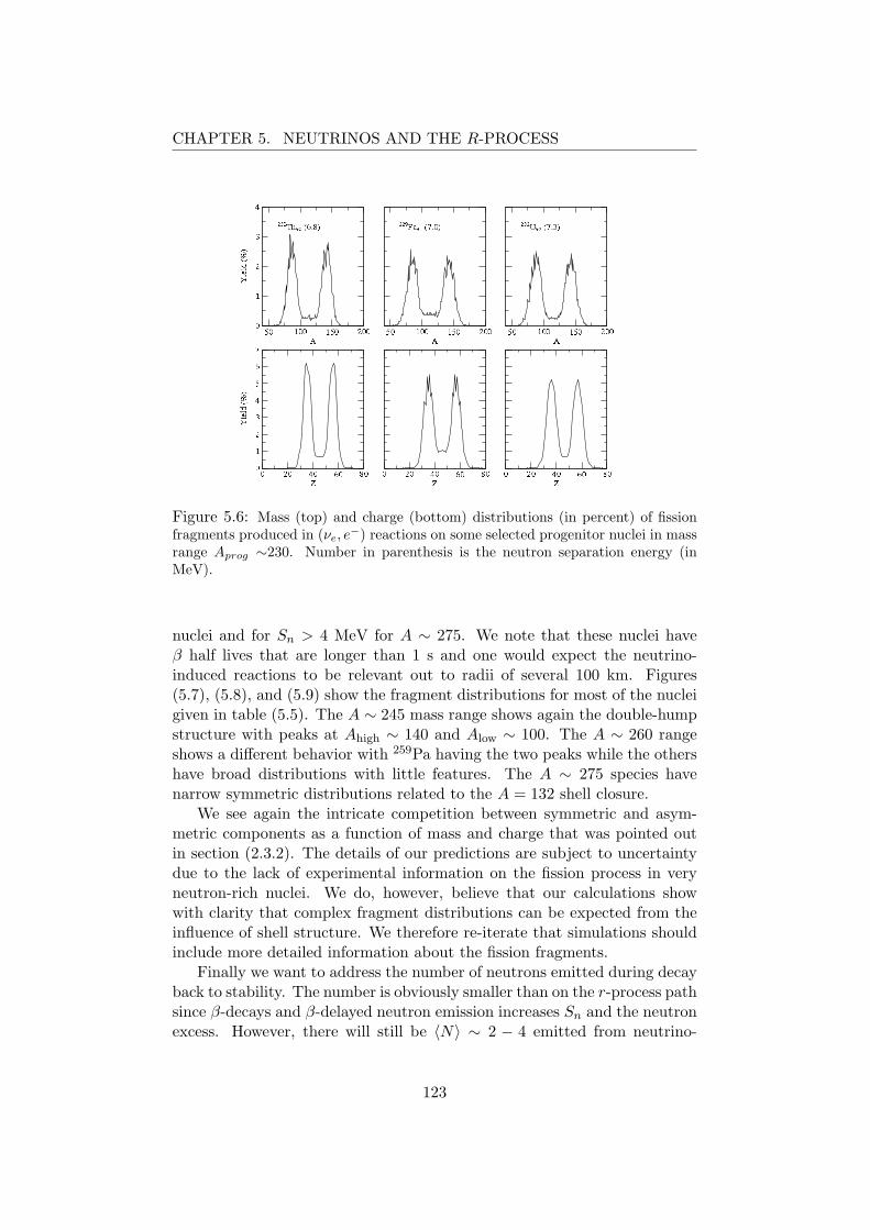
CHAPTER 5. NEUTRINOS AND THE R-PROCESS
Figure 5.6: Mass (top) and charge (bottom) distributions (in percent) of fissionfragments produced in (νe, e
−) reactions on some selected progenitor nuclei in massrange Aprog ∼230. Number in parenthesis is the neutron separation energy (inMeV).
nuclei and for Sn > 4 MeV for A ∼ 275. We note that these nuclei haveβ half lives that are longer than 1 s and one would expect the neutrino-induced reactions to be relevant out to radii of several 100 km. Figures(5.7), (5.8), and (5.9) show the fragment distributions for most of the nucleigiven in table (5.5). The A ∼ 245 mass range shows again the double-humpstructure with peaks at Ahigh ∼ 140 and Alow ∼ 100. The A ∼ 260 rangeshows a different behavior with 259Pa having the two peaks while the othershave broad distributions with little features. The A ∼ 275 species havenarrow symmetric distributions related to the A = 132 shell closure.
We see again the intricate competition between symmetric and asym-metric components as a function of mass and charge that was pointed outin section (2.3.2). The details of our predictions are subject to uncertaintydue to the lack of experimental information on the fission process in veryneutron-rich nuclei. We do, however, believe that our calculations showwith clarity that complex fragment distributions can be expected from theinfluence of shell structure. We therefore re-iterate that simulations shouldinclude more detailed information about the fission fragments.
Finally we want to address the number of neutrons emitted during decayback to stability. The number is obviously smaller than on the r-process pathsince β-decays and β-delayed neutron emission increases Sn and the neutronexcess. However, there will still be 〈N〉 ∼ 2 − 4 emitted from neutrino-
123
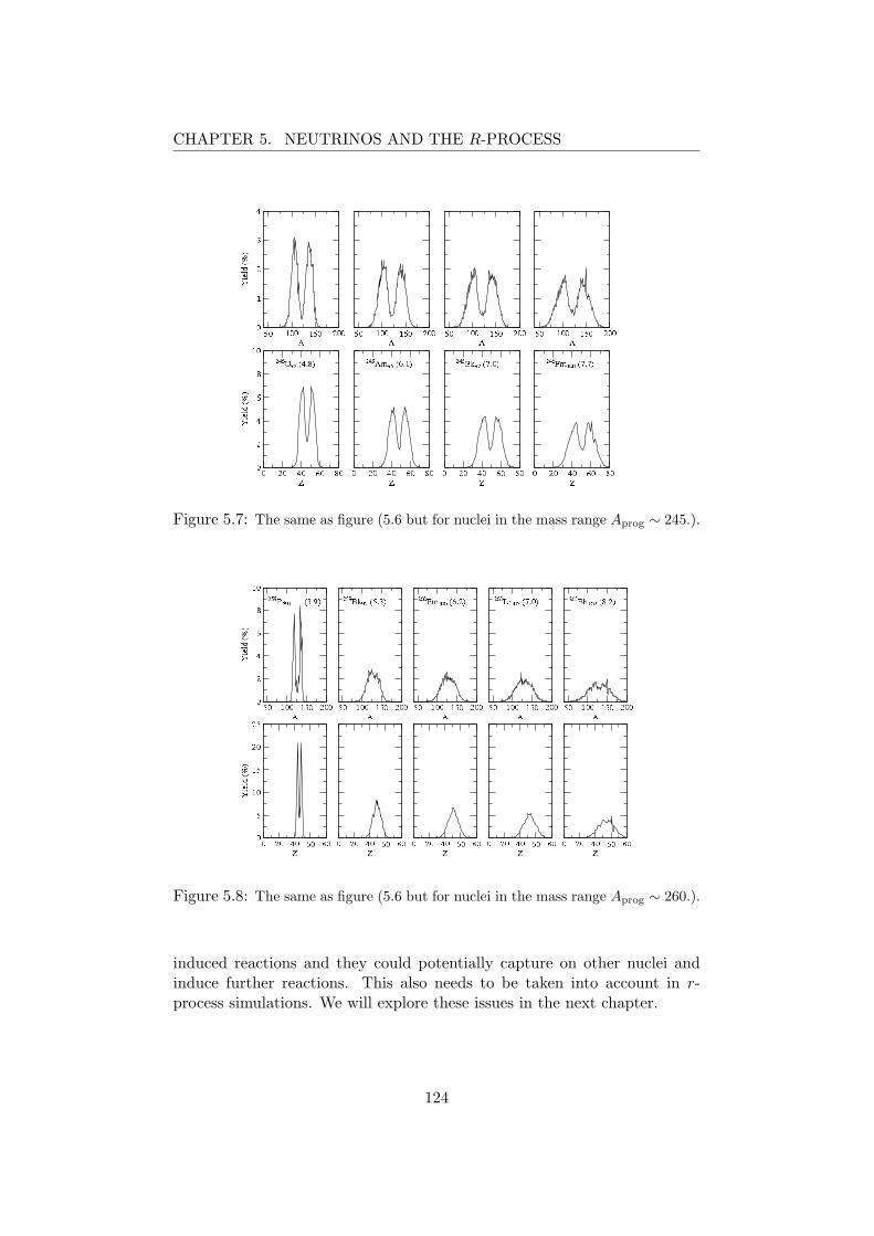
CHAPTER 5. NEUTRINOS AND THE R-PROCESS
Figure 5.7: The same as figure (5.6 but for nuclei in the mass range Aprog ∼ 245.).
Figure 5.8: The same as figure (5.6 but for nuclei in the mass range Aprog ∼ 260.).
induced reactions and they could potentially capture on other nuclei andinduce further reactions. This also needs to be taken into account in r-process simulations. We will explore these issues in the next chapter.
124

CHAPTER 5. NEUTRINOS AND THE R-PROCESS
Figure 5.9: The same as figure (5.6 but for nuclei in the mass range Aprog ∼275.).
5.3.3 Preliminary Conclusions
The results presented above represent a significant improvement over previ-ous studies by using (presumably) more realistic fission barriers and givingthe detailed fragment distributions for the first time. Qian’s proposal seemsto be supported by the fragment peaks from symmetric and asymmetric com-ponents that showed enhancement at A ∼ 90 and A ∼ 135. However, we findnegligible neutrino-induced fission in the mass range Aprog ∼ 200− 215 andonly for Z > 92 will fission become dominant. It therefore appears that thefission probability from neutrino-induced reactions are smaller than assumedby Qian (as was also concluded in [158]). As mentioned above, dynamicalr-process simulations are needed to settle the issue in a proper manner. Thiswill also require us to include β-delayed and neutron-induced processes fora consistent simulation.
The prospect of getting fission cycling from neutrino-induced fission alsolooks slim. The number of neutrons that come out from the reactions issimply not large enough ([158] estimates that between 70 and 100 neutronsper reaction is needed). As noted by Qian, one will have around eight β-decays in the first 10 s after bounce where neutrino fluxes are large. Lookingback on our results for nuclei on the r-process path and those that arelocated between the path and stability, we see that it will be hard to reachnuclei with appreciable fission probabilities and many neutron emissions.For example, in mass range 275 where Zprog ∼ 90 − 92 on the path (table
125

CHAPTER 5. NEUTRINOS AND THE R-PROCESS
(5.3)), we need the charge to increase by 8-10 units for fission to becomedominant according to table (5.5). In agreement with [158], we find thatfission cycling from neutrinos seems out of the question.
126

Chapter 6
Fission and the r-process
6.1 Introduction
The r-process relevant results discussed in the previous chapter gave a pre-liminary idea about the effects of fission. To make these consideration quan-titative we need to implement the nuclear details into full network calcu-lations. The heaviest elements in the r-process network can undergo fis-sion through a number of reactions: neutron-induced, β-induced, neutrino-induced, and spontaneous fission. Having already discussed intensely theneutrino-induced channel, we still need to address the other processes interms of rates, cross sections and fragment distributions. The network cal-culation that we have performed also include the charged particle reactionsthat built up the seed nuclei, on which the excess neutrons are captured,from some initial distribution of nucleons and α-particles. The next sectionwill therefore be devoted to the nuclear physics input that are employed.
6.2 Nuclear Physics Input
Apart from fission and neutrino reactions, the nuclear physics processes thatare included in our calculations are basically inherited from the network ofFreiburghaus et al. [155]. We have, however, used another selection of massmodels. These are the Duflo-Zuker masses [166], the Moller, Nix, and KratzFRDM masses [30], and the ETFSI-Q masses [167, 168]. The similaritiesand differences of these mass compilations will be discussed when we presentour results in the next sections. The neutrino reactions included in thenetwork for A < 200 and Z < 70 are an extension of those given in table(4.1) to cover the neutron-rich region also (although here no antineutrinoreactions are considered as they are Pauli blocked). The neutrino-inducedfission and neutron emission reactions described in the previous chapter arein the network for all nuclei with Z = 70−120 from stability to the neutrondrip-line. We will now discuss the other fission channels in some detail and
127
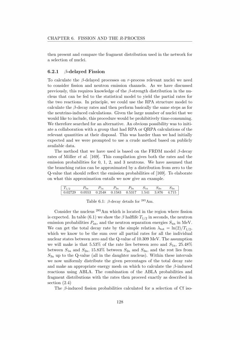
CHAPTER 6. FISSION AND THE R-PROCESS
then present and compare the fragment distribution used in the network fora selection of nuclei.
6.2.1 β-delayed Fission
To calculate the β-delayed processes on r-process relevant nuclei we needto consider fission and neutron emission channels. As we have discussedpreviously, this requires knowledge of the β-strength distribution in the nu-cleus that can be fed to the statistical model to yield the partial rates forthe two reactions. In principle, we could use the RPA structure model tocalculate the β-decay rates and then perform basically the same steps as forthe neutrino-induced calculations. Given the large number of nuclei that wewould like to include, this procedure would be prohibitively time-consuming.We therefore searched for an alternative. An obvious possibility was to initi-ate a collaboration with a group that had RPA or QRPA calculations of therelevant quantities at their disposal. This was harder than we had initiallyexpected and we were prompted to use a crude method based on publiclyavailable data.
The method that we have used is based on the FRDM model β-decayrates of Moller et al. [169]. This compilation gives both the rates and theemission probabilities for 0, 1, 2, and 3 neutrons. We have assumed thatthe branching ratios can be approximated by a distribution from zero to theQ-value that should reflect the emission probabilities of [169]. To elaborateon what this approximation entails we now give an example.
T1/2 P0n P1n P2n P3n S1n S2n S3n
0.02729 0.0553 0.2548 0.1583 0.5317 1.541 3.876 4.715
Table 6.1: β-decay details for 285Am.
Consider the nucleus 285Am which is located in the region where fissionis expected. In table (6.1) we show the β halflife T1/2 in seconds, the neutronemission probabilities Pxn, and the neutron separation energies Sxn in MeV.We can get the total decay rate by the simple relation λtot = ln(2)/T1/2,which we know to be the sum over all partial rates for all the individualnuclear states between zero and the Q-value of 10.309 MeV. The assumptionwe will make is that 5.53% of the rate lies between zero and S1n, 25.48%between S1n and S2n, 15.83% between S2n and S3n, and the rest lies fromS3n up to the Q-value (all in the daughter nucleus). Within these intervalswe now uniformly distribute the given percentages of the total decay rateand make an appropriate energy mesh on which to calculate the β-inducedreactions using ABLA. The combination of the ABLA probabilities andfragment distributions with the rates then proceed exactly as described insection (2.4)
The β-induced fission probabilities calculated for a selection of Cf iso-
128
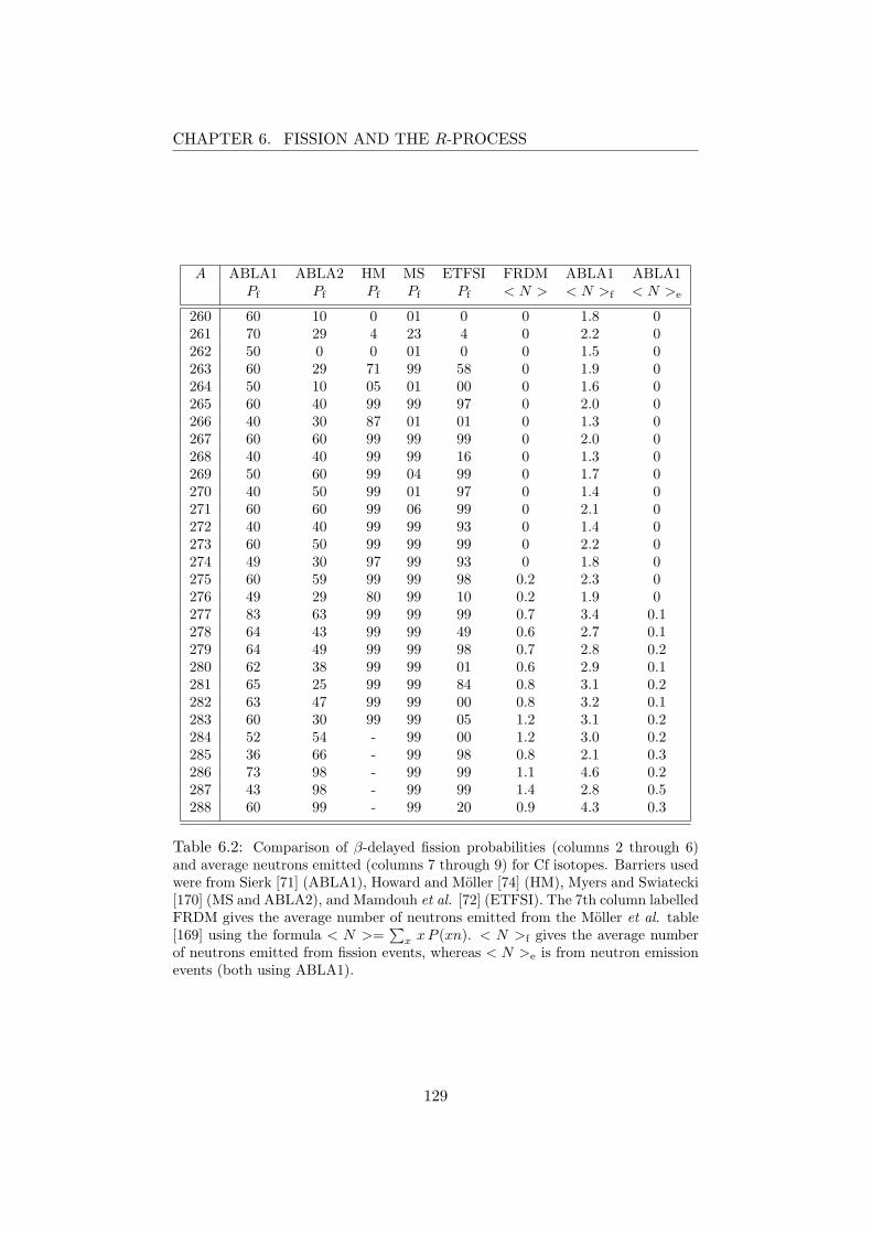
CHAPTER 6. FISSION AND THE R-PROCESS
A ABLA1 ABLA2 HM MS ETFSI FRDM ABLA1 ABLA1Pf Pf Pf Pf Pf < N > < N >f < N >e
260 60 10 0 01 0 0 1.8 0261 70 29 4 23 4 0 2.2 0262 50 0 0 01 0 0 1.5 0263 60 29 71 99 58 0 1.9 0264 50 10 05 01 00 0 1.6 0265 60 40 99 99 97 0 2.0 0266 40 30 87 01 01 0 1.3 0267 60 60 99 99 99 0 2.0 0268 40 40 99 99 16 0 1.3 0269 50 60 99 04 99 0 1.7 0270 40 50 99 01 97 0 1.4 0271 60 60 99 06 99 0 2.1 0272 40 40 99 99 93 0 1.4 0273 60 50 99 99 99 0 2.2 0274 49 30 97 99 93 0 1.8 0275 60 59 99 99 98 0.2 2.3 0276 49 29 80 99 10 0.2 1.9 0277 83 63 99 99 99 0.7 3.4 0.1278 64 43 99 99 49 0.6 2.7 0.1279 64 49 99 99 98 0.7 2.8 0.2280 62 38 99 99 01 0.6 2.9 0.1281 65 25 99 99 84 0.8 3.1 0.2282 63 47 99 99 00 0.8 3.2 0.1283 60 30 99 99 05 1.2 3.1 0.2284 52 54 - 99 00 1.2 3.0 0.2285 36 66 - 99 98 0.8 2.1 0.3286 73 98 - 99 99 1.1 4.6 0.2287 43 98 - 99 99 1.4 2.8 0.5288 60 99 - 99 20 0.9 4.3 0.3
Table 6.2: Comparison of β-delayed fission probabilities (columns 2 through 6)and average neutrons emitted (columns 7 through 9) for Cf isotopes. Barriers usedwere from Sierk [71] (ABLA1), Howard and Moller [74] (HM), Myers and Swiatecki[170] (MS and ABLA2), and Mamdouh et al. [72] (ETFSI). The 7th column labelledFRDM gives the average number of neutrons emitted from the Moller et al. table[169] using the formula < N >=
∑x xP (xn). < N >f gives the average number
of neutrons emitted from fission events, whereas < N >e is from neutron emissionevents (both using ABLA1).
129
CHAPTER 6. FISSION AND THE R-PROCESS
topes are presented in table (6.2) and compared to those given in table 2 of[163]. The column ABLA1 shows the calculation using the Sierk barriers [71](FRDM mass model), whereas ABLA2 uses the Thomas-Fermi barriers andmasses of [170]. We see that the two ABLA calculations yield rather similarnumbers, and that the odd-even effects are smaller than for the MsSw andETFSI barriers. The HM barriers give the highest fission probabilities whichis expected since they are generally lower. Recalling the inconsistencies ofthe HM and ETFSI barriers discussed in section (2.3.1), we are more inclinedto trust the MS barriers. It is therefore nice to see similar trends for ABLA2and MS. However, our results are mostly below the other calculations andwe find about equal probabilities for fission and neutron emission(s) in manycases. This tells us that the assumption used in many r-process studies ofPfission = 1 above A ∼ 245 (see discussion and references in [163]) should bemore carefully examined. We will address this question again below whenwe consider the importance of the different fission channels.
In the last columns of table (6.2) we give the average number of neutronsemitted according to a simple estimate from the Moller et al. table (see thetable caption) and the number from fission and neutron evaporation eventscalculated with ABLA using FRDM masses and Sierk barriers (the sum ofthese two numbers gives the average for a β-induced reaction). We see thatthe FRDM estimate and the neutron evaporation in ABLA have similartrends with FRDM lying 0.5-1.0 neutrons above ABLA. However, if we sumboth ABLA numbers we see that these are always larger. This is quitelikely caused by the evaporation taking place in the fission fragments asthey are generally closer to the drip-line than the parent nucleus. Since wedo not have the number of neutrons emitted in fission events with the othermethods, this comparison would seem unfair. We do, however, stress againthat these effects should be put in the network as the neutrons released caninduce further reactions (we will elaborate on this issue below).
6.2.2 Neutron-induced and Spontaneous Fission
Neutron-induced reactions could in principle be calculated with the ABLAcode if one had the strength distribution for (n, γ) reactions on the nuclei(which is normally obtained from the inverse reaction through detailed bal-ance). However, since this information was not accessible on a reasonabletimescale, we had to find another solution. We did have the neutron-inducedfission rates from [163] and therefore only the fragment distributions wereneeded. For that purpose one needs a sensible guess of the strength distribu-tion. Here we employed the presumably simplest method one can think of.We assume that the entire strength is located at Sn in the (A+1, Z) nucleus.This gave us an energy as input for ABLA. We further assumed zero angularmomentum as this has little influence as discussed in section (2.4). In orderto get the fragment distribution in this fashion, we are only interested in
130
CHAPTER 6. FISSION AND THE R-PROCESS
the fission channel (neutron emission is basically the (γ, n) reaction whichis already in the network). Therefore we forced ABLA to simulate fissionevents by putting all other channels to zero.
Spontaneous fission is also expected to have importance and we needto have a description of this as well. Here we have used the experimentalvalue when available. For nuclei where there is no experimental informationwe use a formula obtained from a regression fit to the data (see [171] andreferences therein),
log Tsf = 8.0Bf − 21.5, (6.1)
where the half life is measured in seconds and the fission barrier Bf is inMeV. The barriers used in the formula are always those of MS [170]. Thereare of course several issues with this crude approach to the spontaneousfission half life. We will discuss some possible future improvements of thisdescription in the next chapter.
The work on r-process nucleosynthesis in [171] also used an empiricalformula for the fragment distributions. The expression used was
YAf ,Zf(Z,A) ∝ exp
(−(Z − ZA)2/cZ
)×
[exp
(−(A−AL)2/cA
)+ exp
(−(A−AH)2/cA
)],(6.2)
where cZ and cA are the widths, and ZA, AL, and AH are specific functionsof the mass Af and charge Zf of the fissioning nucleus. The formula is thusseen to contain a single gaussian for the charge and a two gaussian sumfor the mass. While this is adequate in some regions (f.x. around uraniumand thorium), we have repeatedly argued that this picture now appearstoo simplistic. In the next section we will show some specific examplesthat contrast the formula above with the results from ABLA. Despite theseproblems we will still employ eq. (6.2) for spontaneous fission yields.
6.2.3 Fragment Distributions
The fission fragment distributions for two examples of Am isotopes areshown in figures (6.1) and (6.2). The two were chosen since they play rolesat different times during the r-process simulations that we will discuss be-low. As one can see, the ABLA yield from all processes are qualitativelyvery different. For all processes displayed we see a single-hump structure in275Am, whereas 287Am shows a much more complicated pattern with fourpeaks for β- and neutron-induced fission, and a double-hump for neutrino-induced fission. This should be less surprising as we have already seen insection (2.3.2) that the profiles can change dramatically within an isotopicchain, and with excitation energy.
We see clearly that β- and neutron-induced yields are very similar. Thisfact is to be expected since the strength is located at roughly the sameenergies (around and below 5 MeV in both species). The number of neutrons
131
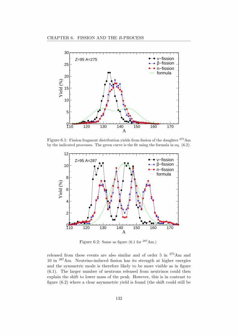
CHAPTER 6. FISSION AND THE R-PROCESS
110 120 130 140 150 160 170A
0
5
10
15
20
25
30
Yie
ld (
%)
ν−fissionβ−fissionn−fissionformula
Z=95 A=275
Figure 6.1: Fission fragment distribution yields from fission of the daughter 275Amby the indicated processes. The green curve is the fit using the formula in eq. (6.2).
110 120 130 140 150 160 170A
0
2
4
6
8
10
12
Yie
ld (
%)
ν−fissionβ−fissionn−fissionformula
Z=95 A=287
Figure 6.2: Same as figure (6.1 for 287Am.)
released from these events are also similar and of order 5 in 275Am and10 in 287Am. Neutrino-induced fission has its strength at higher energiesand the symmetric mode is therefore likely to be more visible as in figure(6.1). The larger number of neutrons released from neutrinos could thenexplain the shift to lower mass of the peak. However, this is in contrast tofigure (6.2) where a clear asymmetric yield is found (the shift could still be
132
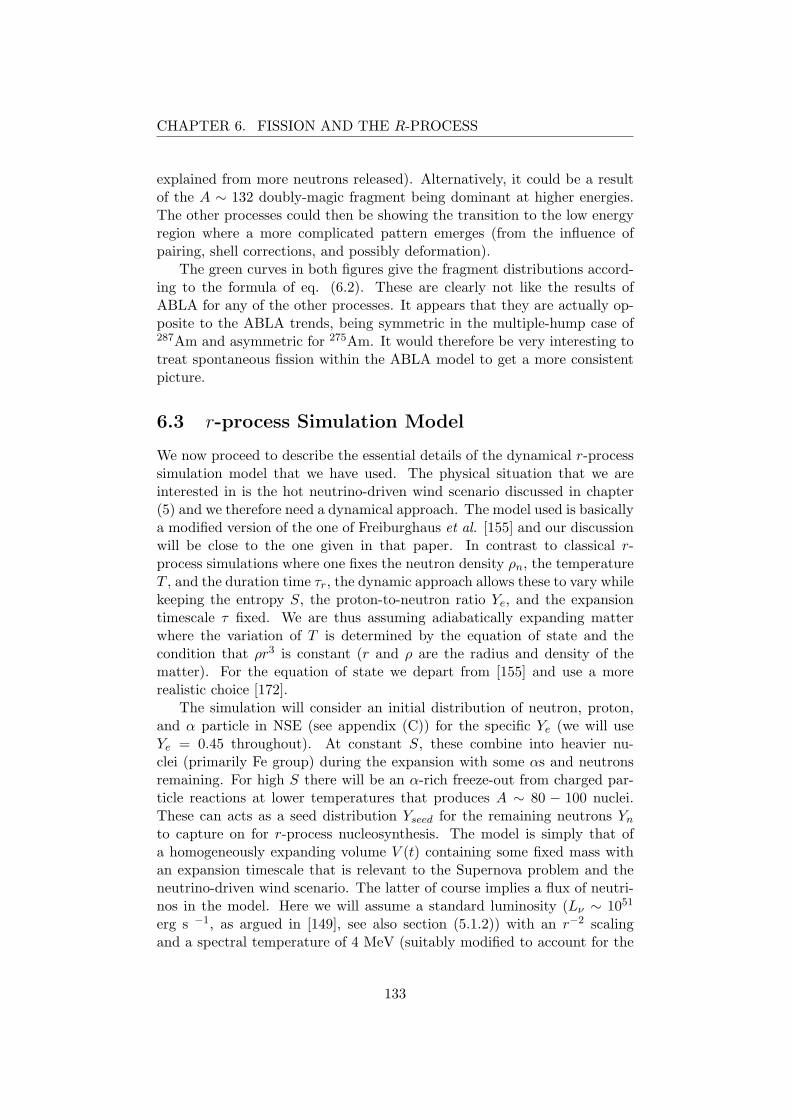
CHAPTER 6. FISSION AND THE R-PROCESS
explained from more neutrons released). Alternatively, it could be a resultof the A ∼ 132 doubly-magic fragment being dominant at higher energies.The other processes could then be showing the transition to the low energyregion where a more complicated pattern emerges (from the influence ofpairing, shell corrections, and possibly deformation).
The green curves in both figures give the fragment distributions accord-ing to the formula of eq. (6.2). These are clearly not like the results ofABLA for any of the other processes. It appears that they are actually op-posite to the ABLA trends, being symmetric in the multiple-hump case of287Am and asymmetric for 275Am. It would therefore be very interesting totreat spontaneous fission within the ABLA model to get a more consistentpicture.
6.3 r-process Simulation Model
We now proceed to describe the essential details of the dynamical r-processsimulation model that we have used. The physical situation that we areinterested in is the hot neutrino-driven wind scenario discussed in chapter(5) and we therefore need a dynamical approach. The model used is basicallya modified version of the one of Freiburghaus et al. [155] and our discussionwill be close to the one given in that paper. In contrast to classical r-process simulations where one fixes the neutron density ρn, the temperatureT , and the duration time τr, the dynamic approach allows these to vary whilekeeping the entropy S, the proton-to-neutron ratio Ye, and the expansiontimescale τ fixed. We are thus assuming adiabatically expanding matterwhere the variation of T is determined by the equation of state and thecondition that ρr3 is constant (r and ρ are the radius and density of thematter). For the equation of state we depart from [155] and use a morerealistic choice [172].
The simulation will consider an initial distribution of neutron, proton,and α particle in NSE (see appendix (C)) for the specific Ye (we will useYe = 0.45 throughout). At constant S, these combine into heavier nu-clei (primarily Fe group) during the expansion with some αs and neutronsremaining. For high S there will be an α-rich freeze-out from charged par-ticle reactions at lower temperatures that produces A ∼ 80 − 100 nuclei.These can acts as a seed distribution Yseed for the remaining neutrons Yn
to capture on for r-process nucleosynthesis. The model is simply that ofa homogeneously expanding volume V (t) containing some fixed mass withan expansion timescale that is relevant to the Supernova problem and theneutrino-driven wind scenario. The latter of course implies a flux of neutri-nos in the model. Here we will assume a standard luminosity (Lν ∼ 1051
erg s −1, as argued in [149], see also section (5.1.2)) with an r−2 scalingand a spectral temperature of 4 MeV (suitably modified to account for the
133

CHAPTER 6. FISSION AND THE R-PROCESS
red-shift effect of the protoneutron star).During the adiabatic expansion we have the standard thermodynamic
identity
T (t) = T0
[V0
V (t)
]γ−1
(6.3)
with adiabatic exponent γ and otherwise obvious notation. Since we arefurthermore assuming a uniform expansion with constant velocity, we havefor the radius r(t) = r0 + vt with v the expansion velocity. For the initialcondition we follow [155] and assume T0 = 9 × 10⁹ K, r0 = 130 km, andv = 4500 km s −1. Defining the expansion timescale by T (τ) = T0/e weget τ = 50 ms for the mentioned velocity (with γ = 4/3 since radiationdominates the entropy).
A change in the expansion timescale τ would have a direct effect on thevery important quantity Yn/Yseed. This ratio was already discussed in sec-tion (5.1.2) where we argued that it needs to be 100 or more to accountfor heavy nuclei including the actinides. If τ becomes shorter (for largerexpansion velocities) then one will actually increase Yn/Yseed. This is aconsequence of the α particles having less time to break the 3α and ααnbottlenecks, resulting in less heavy nuclei and more neutrons for them tocapture. Turning this argument around we conclude that shorter timescalesrequire smaller S to produce even the heaviest elements ([146] has an exten-sive discussion of these issues),
The advantage of this adiabatically expanding model over the classicalr-process simulation should be clear when considering our preferred site.It takes the changes in the r-process path with T and the possible non-equilibrium of the (n, γ) reactions during freeze-out into account.
6.4 Results
We now present the results of the r-process fission studies. These have beencarried out in a parametric way where we have varied the initial entropy tosee the effects. We have also studied the influence of different mass modelsand found some very interesting features. The importance of the differentfission channels will be addressed, also within different mass models. Lastlywe will comment on some issues of consistency of theoretical inputs in thistype of study.
6.4.1 The Region and Role of Fission
First we will discuss the region where fission takes place in the r-process.For this purpose we show a detailed contour plot of the fission barriers fromthe Thomas-Fermi model of [170] in figure (6.3). For all the mass modelsshown we clearly see the influence of the N = 184 shell closure. When the
134

CHAPTER 6. FISSION AND THE R-PROCESS
r-process reaches charges Z ∼ 85 − 90 the matter will accumulate at thismagic number where large fission barriers are found. Fission can thereforeonly occur for nuclei that manage to pass this waiting-point. This dependson the strength of the shell gap of the particular mass model and also onthe β half lives (we will explore this effect below). We see the weakest gapin the Duflo-Zuker masses, followed by FRDM, and with the ETFSI modelshowing the strongest gap. This results in slightly less fission for the ETFSImodel compared to the other two (we will quantify this below).
140 150 160 170 180 190 200 210 220 230N
85
90
95
100
105
110
Z
-2 0 2 4 6 8 10
1098
7
7
77
66
6
6
5
55
5
5
54
4
4
4
44
3
33
3
3 2
2
2
2
11
1
0
140 150 160 170 180 190 200 210 220 230N
85
90
95
100
105
110
Z
FRDMDuflo ZukerETFSI
Figure 6.3: Region of the nuclear chart where fission takes place during the r-process. The contour lines represent the Thomas-Fermi fission barrier heights inMeV. Crosses show the nuclei for which neutron-induced fission dominates over(n, γ) (based on [163]). Diamonds show the nuclei for which the spontaneous fissionor β-delayed fission operates in a time scale smaller than 1 second (the former basedon [171], the latter based on the method of section (6.2.1)). The lines show thelocation for which negative neutron separation energies are found in different massmodels (FRDM [30], ETFSI [167] and Duflo-Zuker [166]).
Once the matter reaches high enough Z to fission it will mainly occurthrough the neutron-induced channel, as we will discuss shortly. The eventwill generally release many neutrons (more than 10 on the r-process pathand around 6 when fission happens after freeze-out). Most of these neutronscome from the fission fragments which will lie closer to the drip-line thanthe parent nucleus. These neutrons can then be recaptured by other, mainlyheavy nuclei (since the cross sections are larger). We can therefore have achain-reaction effect that fissions the heavy material on a timescale of afew seconds. This will also be the case after ρn drops and the r-process
135

CHAPTER 6. FISSION AND THE R-PROCESS
effectively ends since the matter at N = 184 will β-decay toward ’stability’and produce further β-delayed neutrons. We note that these qualitativeconsiderations are independent of the fission barriers (see for example [173]where a similar figure for the ETFSI barriers [72] is given).
The fragment distributions shown in figures (6.1) and (6.2) are veryappropriate with respect to the discussion above as they are located in thetwo different places where fission can take place. 287Am is encountered onthe r-process path, whereas 275Am is on the decay back to stability afterfreeze-out. It is therefore interesting to consider the very different yieldprofiles. For 287Am the fragments at A < 130 and A ∼ 160 could contributeto the low end of the A ∼ 130 2nd r-process peak and the small peak atA ∼ 160 (expected to come from fission since the early work of [152]). In275Am we have two fragments in the high part of the A ∼ 130 peak. Wethus see that the heavier nuclei will give fragments that are lighter thanthe less neutron-rich ones. The endpoint of the r-process might thereforebe important for the A < 130 region where the UMP measurements showinteresting deviations from solar abundances.
Figure 6.4: Abundance pattern of an r-process simulation after around 1 s. Upperpanel shows the mass abundance profiles on a logarithmic scale. A contour plot ofthe relevant part of the nuclear chart is shown in the lower panel. The simulationused the FRDM masses [30] and had S = 400 (Yn/Yseed = 186).
In figure (6.4) we show a snapshot of a simulation using the FRDM massmodel. The parameters are S = 400 or Yn/Yseed = 186. The distributionof nuclei is shown roughly one second after the simulation was begun (whenthe nuclei reach the fission region). From the contour color coding and theabundance pattern one clearly sees the shell closures at N = 82, 126, and
136

CHAPTER 6. FISSION AND THE R-PROCESS
184 (minor shells are also seen just below N = 184, see the FRDM partof figure (6.8)). As discussed above, we see the accumulation of matterhappening at N = 184 for Z ∼ 90−95 and also the matter that has climbedabove the shell closure to A ∼ 285. The endpoint of the r-process is seento be around A ∼ 280 (this turns out to be true for all the mass modelsused). The nuclei above A ∼ 200 (except actinides) will of course decay,the heaviest ones doing so through fission to produce fragments in the rangeA = 130 − 190. This does, however, depend on the particular mass modelused as we will discuss below.
10−7
10−6
10−5
10−4
10−3
10−2
10−1
100
Yn
0 1 2 3 4 5 6 7 8 9 10Time (s)
0.0e+00
1.0e−04
2.0e−04
3.0e−04
4.0e−04
5.0e−04
6.0e−04
7.0e−04
dYfis
s/dt (
s−1 )
n−fissionbeta−fissionnu−fissionTotalTotal Integrated
Yn
Figure 6.5: The influence of the different fission channels as a function of time.Shown are differential contributions dYfiss
dt (left axis) for neutron-induced (red), β-induced (green), neutrino-induced (dark blue), and total (black). The integratedtotal (light blue) and Yn (purple) are also displayed (right axis). The simulationused the FRDM masses [30] and had S = 400 (Yn/Yseed = 186).
The timescale and periods of fission is illustrated in figure (6.5) where theabundance changes due to the various fission channels are plotted along withYn. The total is clearly seen to be dominated by neutron-induced fission withvery little contribution from β-induced and virtually no neutrino-induced.This holds true for all mass models as one can see from table (6.3) whichgives the relative contributions for different values of the entropy S. We seethat the contributions of different fission channels are increasing with S andgenerally very similar for the different mass models (except for ETFSI-Q atS = 350, see below).
Figure (6.5) shows two characteristic periods. There is an initial phase(up to about 1 s) where fission takes place at and above the N = 184 peakas discussed above. After the neutron density drops the matter will startto β-decay back to stability and release neutrons that can induce further
137
CHAPTER 6. FISSION AND THE R-PROCESS
S = 350 (Yn/Yseed = 116) (n,fission) β-induced ν-induced Total
ETFSI-Q 0 0 0 0FRDM 10 1 0 11
Duflo-Zuker 10 1 0 11
S = 400 (Yn/Yseed = 186) (n,fission) β-induced ν-induced Total
ETFSI-Q 33 5 0 38FRDM 36 3 0 39
Duflo-Zuker 36 3 0 39
S = 500 (Yn/Yseed = 417) (n,fission) β-induced ν-induced Total
ETFSI-Q 56 4 0 60FRDM 58 5 0 63
Duflo-Zuker 58 5 0 63
Table 6.3: Percentages of different fission channel for different mass models andvarious entropies (or Yn/Yseed).
fission. This is seen as a 2-3 second period where neutron-induced fissionis high and Yn drops only slowly. This dominance of neutron-induced overβ-induced and spontaneous fission is a consequence of its timescale duringthe first seconds of the simulation. Here the neutron density is around 1018
cm −3 and above which gives a lifetime for neutron capture of order a few ms,whereas the β-half lives are an order of magnitude larger. For spontaneousfission the simple formula in eq. (6.1) predicts that the barriers should bearound 2 MeV or below to compete. According to figure (6.3) this wouldrequire Z & 97 during the decay back to stability which seems unrealistic.These timescale considerations were also found to be independent of thebarriers, although they can be quite dependent on the mass model used andparticularly the β-decay properties.
6.4.2 The N = 184 Shell and Half lives
The discussion above made it clear that the N = 184 shell closure has adecisive role in the fission dynamics of the r-process in our simulations. Herewe find the mentioned accumulation of matter occurring for all the massmodels explored. The neutrons that are released from β-delayed neutronemission will start the fission chain reactions described in section (6.4.1).The lifetime against β-decay in the region is therefore important.
To elaborate on this dependence, we have performed calculations wherethe half lives are scaled to make them both longer and shorter than standardvalues. In figure (6.6) we show the results of these simulations. Evidently,the longer half lives have a major influence on the A ∼ 195 peak and alsoon the actinide abundances. This is a result of the drop in neutron densities(down to around 1018 cm −3) that happens while waiting for the β-decays.This produces a weak r-process or strong s-process peak that is shifted tothe right. The severe depletion of the actinide region is also very unfortunateas this would change the U/Th cosmochronometers. For the reduced half
138

CHAPTER 6. FISSION AND THE R-PROCESS
Figure 6.6: Abundance patterns for an FRDM simulation with S = 400. The bluecurve shows the result with standard β half lives [30]. The red curve shows theresults of multiplying the half lives by 10 and the green curve has half lives thatare divided by a factor 10.
lives we see the opposite tendency with good agreement for actinides and aA ∼ 195 peak that is closer to solar compared to that seen when using thestandard FRDM decay rates [30].
There are good reasons to believe that the actual half lives could beshorter than the FRDM numbers in [30]. The more recent tables of [169]which include also forbidden transitions show shorter half lives in the N =184 region of interest. Similar efforts to include forbidden transitions in thehalf lives within a QRPA model are reported in [174] and [175] where ashortening of the half lives by factors of 2-5 compared to those given in [169]is found. This points in the direction of the green curve of figure (6.6) andfurther investigation into this issue is under way.
6.4.3 The N = 82 Shell Closure
In this section we present results for the influence of the shell structureat lower neutron numbers. We have calculated the r-process abundancesfor the different mass models after 1.6 Gy when all decay toward stabilityhas ceased (except for naturally occurring radioactivity). These results areshown in figure (6.7) as a function of entropy S. The profiles shown forFRDM and Duflo-Zuker masses are very similar, whereas that for ETFSI-Q clearly differs. This is related to the shell closures at N = 126 and(particularly) N = 82 which are quenched in ETFSI-Q. The other two havestrong shell gaps also close to the drip-line. This can be clearly seen in figure
139

CHAPTER 6. FISSION AND THE R-PROCESS
(6.8) where the r-process path at freeze-out is shown for the mass models.The conditions of figure (6.7) have almost no gap at N = 82 for the EFTSI-Q masses and the matter therefore passes right through. This means thatmost neutrons are stuck in heavy nuclei and cannot induce fission events.
Figure 6.7: Final r-process abundances (after 1.6 Gy) obtained using differentmass models (FRDM [30], ETFSI-Q [168] and Duflo-Zuker [166]). The solid circlescorrespond to a scaled solar r-process abundance distribution [176].
For the other mass tables there is some accumulation of matter atN = 82and N = 126 and when this matter finally reaches the fission region there arestill many neutrons around to induce fission and release even more neutrons
140
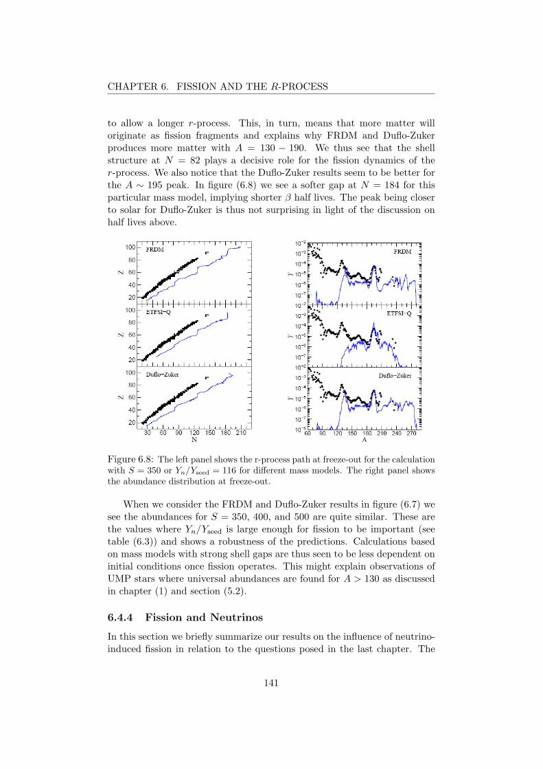
CHAPTER 6. FISSION AND THE R-PROCESS
to allow a longer r-process. This, in turn, means that more matter willoriginate as fission fragments and explains why FRDM and Duflo-Zukerproduces more matter with A = 130 − 190. We thus see that the shellstructure at N = 82 plays a decisive role for the fission dynamics of ther-process. We also notice that the Duflo-Zuker results seem to be better forthe A ∼ 195 peak. In figure (6.8) we see a softer gap at N = 184 for thisparticular mass model, implying shorter β half lives. The peak being closerto solar for Duflo-Zuker is thus not surprising in light of the discussion onhalf lives above.
Figure 6.8: The left panel shows the r-process path at freeze-out for the calculationwith S = 350 or Yn/Yseed = 116 for different mass models. The right panel showsthe abundance distribution at freeze-out.
When we consider the FRDM and Duflo-Zuker results in figure (6.7) wesee the abundances for S = 350, 400, and 500 are quite similar. These arethe values where Yn/Yseed is large enough for fission to be important (seetable (6.3)) and shows a robustness of the predictions. Calculations basedon mass models with strong shell gaps are thus seen to be less dependent oninitial conditions once fission operates. This might explain observations ofUMP stars where universal abundances are found for A > 130 as discussedin chapter (1) and section (5.2).
6.4.4 Fission and Neutrinos
In this section we briefly summarize our results on the influence of neutrino-induced fission in relation to the questions posed in the last chapter. The
141

CHAPTER 6. FISSION AND THE R-PROCESS
clear conclusion from the results presented in this chapter is that fissionthrough neutrinos does not appear to have any significant effect on the r-process under normal circumstances. One could of course imagine an astro-physical site with luminosities different from the standard one assumed forthe neutrino-driven wind. To investigate this possibility, calculations withlarger Lν were carried out. In figure (6.9) we show the results with a factorof 5 and 10 on the neutrino fluence (which basically means multiplication ofLν by the same factor). This figure clearly shows that such increases are notviable as they destroy the ability to produce heavy r-process nuclei (this isthe α-effect discussed by [47] and [177]. See also figure (5.1)).
Figure 6.9: The effects of increasing the neutrino fluency for a simulation with theFRDM mass model and S = 400.
6.5 Nuclear Data Consistence
We have now discussed our results with respect to three different mass mod-els. However, these were all obtained with the Thomas-Fermi fission barriersof [170]. This is of course not quite consistent. We do not expect that therewill be major changes when considering other barriers also but further stud-ies will have to be done. Unfortunately there are some mass tables thatare not extended beyond A ∼ 300 which is what one needs. While sortingout these difficulties one can still do parameter-like studies on the barriersby combining the mass models above with the various barrier compilationsmentioned in this and the last chapter. Ultimately one would of course liketo have all quantities including masses, β half lives, barriers, and fission
142

CHAPTER 6. FISSION AND THE R-PROCESS
yields from a single model but this is still to come.With respect to neutron-induced fission there is still the issue of the sim-
ple placement of the strength discussed in section (6.2.2). This can be im-proved by taking a realistic strength distribution and calculating the ABLAoutcome as mentioned above. Such calculations are currently under way.Through an improvement of the treatment of low-energy barrier penetrationone would also be able to calculate spontaneous fission yields with ABLA,although the half lives still need to be introduced from the outside.
6.6 Concluding Remarks
The studies of fission in the r-process clearly show that mass models are veryimportant. In particular, our results show that the N = 82 shell determinesthe amount of fission taking place during the process. Mass models thathave strong gaps at N = 82 turned out to have very robust abundancepatterns once fission starts operating. The ETFSI-Q mass model thereforeseems to have trouble in describing the influence of fission when compared toFRDM or Duflo-Zuker. We get variations that cannot explain the observedrobustness of the r-process for A ≥ 130. The need for more experimentalmeasurements of the masses in this region is therefore essential. This wouldalso constrain theoretical models and provide a better basis for extrapolationinto the unknown terrain where fission occurs during the r-process.
The discussion on the influence of β half lives at N = 184 showed thatshorter half lives are one of the things needed to get a true r-process peakat A ∼ 195. The need for shorter half lives to avoid accumulation of matterat N = 184 seems to be met by the most recent calculations as discussedabove, but the theoretical models could benefit from stronger constraintscoming from experiment.
We have addressed the issue of fission cycling at several points in thepreceding chapters. The cycling time was estimated to be around 1.5 s inour calculation and since this is of the same order as the duration of ther-process we have no more than one cycle. We therefore expect no influenceof cycling to stabilize the abundance pattern. However, the barriers at theN = 184 are still a concern in this respect. If they are low (and the β halflives are short) then fission cycling could perhaps take place.
The possibility of finding super heavy elements in r-process studies isanother interesting issue. In some simulations we have found nuclei withmasses up to A ∼ 320. However, even if they are present after freeze-out,they will undergo fission during the β-decay back to stability and leave notrace amount. If the barriers were different one could potentially producesome super heavies that would be left over after an r-process. Investigatingthe barrier dependencies could possibly give clues to this intriguing subject.
Finally we mention that the r-process results presented above can also
143

CHAPTER 6. FISSION AND THE R-PROCESS
Figure 6.10: The logarithm of the Uranium to Thorium ratio as a function oftime. The red curve shows the simulation result averaged over FRDM and Duflo-Zuker masses and over entropies S = 350, 400, and 500 where fission contributessignificantly. The measurement for CS 31082-001 is from [179] and that of BD+173248 is from [180].
be used to estimate the age of the oldest stars in the galaxy. This wouldthen put limits on the age of the Milky way and the Universe in general.The recent detection of Th and U in metal-poor stars [178] means that onecan make a more accurate age determination than using the traditional Thto Eu ratio since Th and U are produced through α-decays coming fromthe same mass region. As a simple test we can average the U/Th ratio overS = 350, 400, and 500 for FRDM and Duflo-Zuker and compare to measuredratios. This is done in figure (6.10) where the ratio is plotted as a functionof time. The agreement between the measured values and the simulationcurve is striking, although the uncertainties are still quite large. As arguedin [181], these prediction are very dependent on the inclusion of fission inthe r-process network. In particular, [181] argues that spontaneous fission isespecially important for cosmochronometry using the actinides. Improvingthe description of this channel in the manner outlined above is therefore ahigh priority.
144
Chapter 7
Summary and Outlook
In this thesis we have considered nuclear physics data that are needed formodeling of astrophysical environments. We were particularly concernedwith excitation of nuclei through weak interactions and the subsequent decaythrough various channels. The deexcitation of daughter nuclei was treatedwithin a statistical approach that included particle emissions and fission. Forthe latter reaction our model was also able to determine yield distributionsof fission fragments via a Monte Carlo sampling technique. The calculatednuclear data were then implemented in astrophysical models and the effectsof the new results were discussed.
The first major application treated was the inclusion of neutrino andantineutrino cross sections in early, proton-rich ejecta from core-collapseSupernovae. This environment is a good candidate for the production siteof the rare proton-rich elements that are observed in nature. A very in-teresting new nucleosynthetic flow was discovered when fully including theneutrinos in the nuclear network. It is expected to be generic to proton-rich environments that are traversed by significant neutrino fluxes and wasdubbed the νp-process. Through antineutrino on proton reactions the pro-cess makes neutrons that can overcome the Coulomb barriers and captureon nuclei to help build up proton-rich material with masses between A = 64and A ∼ 100.
Depending on the details of the process, it could likely explain the originof the very rare isotopes 92,94Mo and 96,98Ru which is currently not gener-ally understood. The νp-process is primary, meaning that it produces itsown seeds (contrary to what happen in the well-known s-process). This isconsistent with recent galactic chemical evolution studies [121] that suggesta primary Supernova origin for these proton-rich nuclei.
In a second application of neutrino reactions we considered the role ofneutrino-induced fission reactions in r-process nucleosynthesis. A proposalby Qian [156] attempts to explain recent observations of abundances in verymetal-poor stars by invoking a given amount of neutrino interaction in the
145

CHAPTER 7. SUMMARY AND OUTLOOK
r-process that was responsible for the observed patterns. The suggestionwas that neutrino-induced fission could produce enhanced structure in theabundances at A ∼ 130 and A ∼ 90. However, this requires a high neutrino-induced fission probability during the r-process and on the decay back tostability of the synthesized matter.
We carried out detailed calculations of neutrino-induced processes onnuclei along the r-process path and for representatives on the decay backto stability to evaluate this scenario. Using more realistic barriers than theearlier work of [158], we found that the probabilities are unfavorable. Wedid, however, find that the fragment yields could accommodate those neededin the proposal. Later investigations using dynamical r-process simulationsconfirmed our suspicions that neutrino-induced fission had virtually no effect(less than 1%). The present work therefore rules out the suggestion of Qian[156].
Finally, we considered the general role of fission in the r-process. Forthis purpose we calculated fragment distributions for all relevant nuclei fromneutron-, β-, and neutrino-induced fission. Included was also spontaneousfission based on older work [171]. We found that fission takes place in theregion around the N = 184 shell closure, independent of barriers and massmodels used. The fission events were largely neutron-induced with a smallcontribution from β-induced fission.
The β half lives around this region were instrumental to get a goodreproduction of the 3rd r-process peak at A ∼ 195 (with shorter lifetimesgiving results closer to the observed solar abundances). This was a result ofthe many neutrons that β-decays produce in neutron-rich nuclei with largeQ-values. These could then initiate neutron-induced fission event that wouldalso produce even more neutrons, resulting in a chain reaction mechanism.Longer half lives would then give neutrons off on a longer timescale, shiftingthe 3rd peak to the right (toward the s-process peak).
The r-process simulations were also found to be very sensitive to thestrength of the N = 82 shell gap. The mass models that had a strong gapat N = 82 produced results that were largely independent of the initialcondition whenever the fission region could be reached. For models witha quenching of the shell we found no such convergence. In particular, theEFTSI-Q model [168], which has almost no gap at the drip line, showed poorreproduction of the abundances compared to the FRDM [30] and Duflo-Zuker [166] mass models.
7.1 Outlook - Nuclear Physics
The theoretical nuclear physics that we have used in this thesis is contin-uously subject to revision. Mainly from new experimental data on nuclearproperties that allow one to constrain parameters, but also from new insight
146

CHAPTER 7. SUMMARY AND OUTLOOK
into pure nuclear theory. Throughout the preceding chapters we have al-ready commented on the needed quantities our model requires and we willonly briefly reiterate those that are most important.
The consistency of mass models, barriers etc. that was discussed insection (6.5) is a major concern in nucleosynthesis modeling. We would liketo have one single nuclear framework within which all relevant numbers canbe calculated. Unfortunately this does not exist at the moment. Thereforeone has to be careful with combinations of different data compilations toensure maximum compatibility. Alternatively, one can perform parameterstudies with all the different models to check for obvious inconsistencies.The treatment of fission in the r-process is particularly complicated in thisrespect as the nuclear data need to extend to very high mass numbers.Studies on the influence of other mass models and barrier compilations aretherefore being carried out at the moment.
We have emphasized the importance of β-decay around the magic num-bers. To improve and compare our results for this process we need to con-sider other models for calculating the strength. This work is already inprogress within a QRPA model [174, 175]. The QRPA results give shorterlifetimes around the N = 184 shell which is favorable for the r-process asdiscussed in section (6.4.2). To check the consistency of the simple RPAmodel used for the neutrino capture reactions, we have also calculated theseprocesses within the QRPA. For the test cases considered thus far we see onlysmall deviations between the two approaches. Additional work on β-decaycould also help improve the crude approximation used in section (6.2.1) byproviding the strength distributions. However, due to the rather small in-fluence of β-induced fission in our simulations we do not expect significantchanges in the results from such improvements.
In order to describe spontaneous and neutron-induced fission in a moreconsistent way we also need some improvement in the ABLA code. In par-ticular, low-energy barrier penetration must be taken fully into account.The neutron capture strength and the lifetime against spontaneous fissioncould then be taken from a calculation based on the same masses used inABLA. The combined results would then give a more consistent picture ofthese fission channels.
Another very important feature that one would like to incorporate intothe ABLA method is the quenching of shell closures in the fragment calcu-lations. The softening of shell gaps was only taken into account in the massmodels and the fragments therefore still follow the standard gaps. Includ-ing the quenching will most likely also change the fragments and thus ther-process abundances.
A reaction that we have only briefly touched upon is neutrino-inducedparticle spallation in light nuclei. In the earliest epoch of the Supernovaexplosion there could be considerable effects from inelastic neutrino andantineutrino scattering on light and medium mass nuclei. The subsequent
147

CHAPTER 7. SUMMARY AND OUTLOOK
deexcitation can have high probability for particle emissions and could there-fore influence the nuclear distribution of the material. To consistently in-clude this effect one would also need to calculate the neutral-current reac-tions. These processes can be induced by the other neutrino flavors whichcan have higher average energies. This could then compensate the smallercoupling compared to charged currents (which are roughly a factor of 6larger). It would be interesting to include these in nucleosynthesis studieslike those discussed in chapter (4) for the νp-process.
7.2 Outlook - Nuclear Astrophysics
The νp-process for production of A < 100 proton-rich elements discussed inchapter (4) is believed to be generic. However, to test this belief more workis needed. First of all it would be nice to see a full nucleosynthesis calcula-tion including the entire iron group as in [138] with all neutrino reactionsincluded, and with the different explosion models described in chapter (4).Such calculations are currently in progress.
It would be very interesting to investigate whether the νp-process and ther-process could operate in the same neutrino-wind simulation. The synthesisof light proton-rich nuclei in the wind was discussed already in the work ofFuller and Meyer [47] and also Hoffman et al. [146]. However, no r-processwas found. In the recent work of Wanajo [182] there are indications of bothproton-rich nuclei and r-process matter being synthesized in the same wind(although a rather large neutron star mass of 2M seems to be required).
There are several indications that there are at least two r-process com-ponents needed to reproduce observations [183]. There seems to be differentmechanism needed to produce the nuclei above A ∼ 120 and those belowthis region. A recent study by Kratz et al. [184] indicates that this canbe attributed to different values of the neutron density. They found thatvalues in the range 1020− 1023 cm −3 produce the nuclei with A = 80− 100,whereas the heavier nuclei needed larger densities to be made. An overallgood agreement with the solar abundances could be achieved with an appro-priate superposition of densities up to 1028 cm −3 [184]. The same kind ofsuperposition studies was also done in Freiburghaus et al. [155] where abun-dances from different entropies were combined. The physical origin of suchsuperpositions could be variations in initial conditions from convection, ro-tation or even magnetic fields at the astrophysical production site. It wouldbe very interesting to try similar superpositions with fission included in ther-process network.
In order to really test which features of our astrophysical results are trulygeneric we would like to collaborate with other groups in order to implementthe nuclear data into different simulation models. Hopefully this will givesimilar results of course. Work in this direction is already in progress.
148

CHAPTER 7. SUMMARY AND OUTLOOK
The potential effects of our results on galactic chemical evolution studiesis yet another very interesting direction to explore. The recent findings ofTravaglio et al. [185] suggests a light element primary process that operatesvery early in the Galaxy and is independent of the r-process. The νp-processcould very well be a good candidate for this mechanism. The assumptionthat all core-collapse events will have a νp-process could be tested by calcu-lating the yields for different progenitor star masses and implementing thesein chemical evolution models.
The subject of stellar nucleosynthesis has an intrinsic statistical nature.Many stars of vastly different masses and from various epochs of the Uni-verse contribute to the patterns we observe. The future directions of researchmentioned above are of course dependent on the continued expansion and re-finement of the observational data. A larger number of observed stars wouldalso allow us to infer something about the frequency of stellar events. Im-provements in resolution and in the number of isotopes that can be detectedwould also be a great help to modelers, particularly in the popular field ofcosmochronometry. We need more high quality abundance measurementson interesting stellar objects to work out the details of the grand picture ofnucleosynthesis in our Universe.
149

Appendix A
Formalism and Conventions
A.1 Units and Definitions
Natural units where c = ~ = 1 are used. In some equations where Boltz-mann’s constant enters we will also set kB = 1. The four-vectors usedare given by Aµ = (A0, ~A). The metric is diagonal with positive time-component. It is thus equal to its own inverse and has the explicit form
gµν = gµν = Diag(1,−1,−1,−1). (A.1)
The inner-product of two four-vectors is thus: AµBµ = A0B0 − ~A · ~B =A0B0 −
∑3i=1A
iBi. One also has A0 = A0 and Ai = −Ai.We use the Dirac matrices
β =(
1 00 −1
)~α =
(0 ~σ~σ 0
)(A.2)
and the gamma matrices in the so-called Dirac representation
γ0 = β =(
1 00 −1
)~γ = β~α =
(0 ~σ−~σ 0
)(A.3)
γ5 = γ5 = iγ0γ1γ2γ3 =(
0 11 0
). (A.4)
For the 4x4 spin matrix we leave out the factor of 12
~Σ =(~σ 00 ~σ
)(A.5)
so that helicity ~Σ · p can have the values ±1. The metric is used to raise andlower gamma matrix indices, so that
γµ = gµνγν . (A.6)
150

APPENDIX A. FORMALISM AND CONVENTIONS
This means that γ0 = γ0 and γi = −γi, i = 1, 2, 3.We assume that the neutrino is a massless spin-half Dirac particle. In
this setup it is well-known that the spinor can be chosen as an eigenfunctionof both the helicity ~Σ · p and chirality γ5 [186]. Furthermore, for positiveenergy solutions (needed in the muon capture processes of chapter (3)) theeigenvalues of helicity and chirality are the same. For a neutrino movingalong the positive z-axis, the two possible solution are
ψ = N(χ+
χ+
)exp(i~p · ~x) (A.7)
for positive helicity and chirality and
ψ = N(
χ−−χ−
)exp(i~p · ~x) (A.8)
for negative. Here χ± are the usual Pauli two-spinors and N is a normal-ization constant which is given by N−2 = (2π)32ε, where ε is the neutrinoenergy. We employ the normal Standard Model assumption and take theneutrino to be purely left-handed which is the same as negative helicity.
The isospin formalism used has basis elements for neutron (n) and proton(p) given by
|n〉 =(
10
), |p〉 =
(01
). (A.9)
The SU(2) isospin group that acts on these vectors have generators denotedby ~τ = (τ1, τ2, τ3) = 1
2~σ. These are of course identical to the usual Paulimatrices as indicated and the introduction of a different notation is to avoidany confusion with normal angular momentum. We see that neutrons haveisospin projection (τ3 eigenvalue) 1/2 and protons have projection -1/2.
For a nucleus with A nucleons we define the total isospin in the obviousfashion
T =A∑
i=1
~τi. (A.10)
As for standard angular momentum coupling, the projections merely addand we have
T3 =12(N − Z), (A.11)
where N is the number of neutrons and Z is the number of protons. This isthe important relation needed for the derivation of sum rules in eq. (2.45).
A.2 Angular Momentum Coupling and SphericalFunctions
The angular momentum conventions used are basically those of Edmonds[28]. However, the Clebsch-Gordan coefficients are written with total angu-
151

APPENDIX A. FORMALISM AND CONVENTIONS
lar momentum first and then projection after the separator in the followingfashion
〈J1J2J |J1zJ2zJz〉, (A.12)
where we are coupling J1 and J2 to total angular momentum J . The pro-jections are self-explanatory. The Wigner 3J symbols and the Racah Wsymbols are defined as in [28].
We use the triangle notation ∆(J1J2J), which is one if J1 and J2 canreach J when stepping from J1 +J2 down to |J1−J2| in unit steps and zerootherwise.
The standard square-root factors in angular coupling are defined as [J ] =√2J + 1. We have also used the notation χi = (li− ji)(2ji +1), where i can
be a particle or hole index, li is the orbital angular momentum of i, and jiis the total angular momentum of i.
The vector spherical harmonics are defined by
YMJ,l,1 =
∑µλ
〈l1J |µλM〉Ylµ~eλ, (A.13)
where Ylµ are the usual spherical harmonic with angular momentum l andprojection µ. These function satisfies a number of divergence and curl prop-erties that may be found in [28, 18]. The most important relation needed inchapter (3) is the inversion relation
Ylµ~eλ =∑JM
〈l1J |µλM〉YMJ,l,1, (A.14)
which is obtained by using the unitarity properties of the Clebsch-Gordancoefficients.
The multipole expansion used is given in Walecka appendix B [18]. In-troduce ~ez = ~κ/|~κ| and take the two other basis vectors of 3-space so that~ex, ~ey, ~ez forms a right-handed orthonormal basis. Then introduce thespherical basis vectors
~e0 = ~ez , ~e±1 = ∓ 1√2
(~ex ± i~ey) . (A.15)
These spherical components satisfies the identities
(~eλ)† = (−1)λ~e−λ , (~eλ)† · ~eλ′ = δλ,λ′ . (A.16)
Then the partial wave expansion of the plane wave is given by
exp (i~κ · ~x) =∞∑
J=0
√4π[J ]iJjJ(κx)YJ,0(Ωx). (A.17)
Here the jJ(κx) is the spherical Bessel function of order J and YJ,M (Ωx) isthe spherical harmonic of order J and projection M . We have introduced
152

APPENDIX A. FORMALISM AND CONVENTIONS
the notation |~κ| = κ, |~x| = x and [J ] =√
2J + 1. The product of thespherical basis components and the partial wave expansion is now given bythe expressions
~eλ exp (i~κ · ~x) = − iκ
∞∑J=0
√4π[J ]iJ∇ (jJ(κx)YJ,0(Ωx)) (A.18)
for λ = 0 and
~eλ exp (i~κ · ~x) = −∞∑
J=1
√2π[J ]iJ
[λjJ(κx)Yλ
J,J,1 +1κ∇∧
(jJ(κx)Yλ
J,J,1
)](A.19)
for λ = ±1. Here YMJ,L,1 is the vector spherical harmonic. This represents the
coupling of spherical harmonic YL,m and the spherical basis vectors, whichhave intrinsic angular momentum (1, λ), to total angular momentum (J,M).Now we will need also the conjugate relations to get the plane wave of theopposite sign. For the plane wave alone we have
exp (−iκ · ~x) =∞∑
J=0
√4π[J ](−i)JjJ(κx)YJ,0(Ωx). (A.20)
This follows easily from the fact that the Bessel is real and spherical har-monics (J, 0) are proportional to the Legendre polynomial of order J , whichis also real. For the product of plane wave and spherical basis componentswe get
~eλ exp (−i~κ · ~x) =i
κ
∞∑J=0
√4π[J ](−i)J∇ (jJ(κx)YJ,0(Ωx)) (A.21)
for λ = 0 and
~e−λ exp (−i~κ · ~x) =∞∑
J=1
√2π[J ](−i)J
[λjJ(κx)Y−λ
J,J,1 +1κ∇∧
(jJ(κx)Y−λ
J,J,1
)](A.22)
for λ = ±1. Here we have used (~eλ)† = (−1)λ~e−λ and the following identityfor the vector spherical harmonics(
YMJ,l,1
)†= (−1)l+1−J+MY−M
J,l,1 (A.23)
and the expressions
∇ρ (jJ(ρ)YJ,M (Ωρ)) =
√J + 12J + 1
jJ+1(ρ)~YMJ,J+1,1 +
√J
2J + 1jJ−1(ρ)~YM
J,J−1,1
(A.24)
1κ∇∧
(jJ(κx)~YM
J,J,1
)= −i
√J
2J+1jJ+1(κx)~YMJ,J+1,1
+i√
J+12J+1jJ−1(κx)~YM
J,J−1,1. (A.25)
153

APPENDIX A. FORMALISM AND CONVENTIONS
A.3 Spherical Dirac Equation
We assume that the potential origination from the nucleus is sphericallysymmetric and minimally coupled. Separation of the Dirac equation inspherical coordinates may therefore be performed (see example 9.3 of [186]).This yields the following wave function
φjm =(
ig(r)Ωjlm(r)−f(r)Ωjl′m(r)
), (A.26)
where |l− l′| = 1 since the two components have opposite parity [186]. Theradial functions fulfill the following equations
ddr
(gf
)=(
−1+κr E +m− V (r)
−E +m+ V (r) −1−κr
)(gf
), (A.27)
where
κ =−(l + 1) , j = l + 1
2l , j = l − 1
2
(A.28)
andΩj,l,m(r) =
∑ml,ms
(l, 12 , j|ml,ms,m)Yl,ml
(r)χms (A.29)
is the coupling of Pauli two-spinor, χms , and spherical harmonic, Yl,ml, to
total angular momentum j. From the properties of the Clebsch-Gordan co-efficients it follows that Ω†j,l,mΩj′,l′,m′ = δj,j′δl,l′δm,m′ so that the requirementof normalization becomes∫ ∞
0r2dr(|g|2 + |f |2) = 1. (A.30)
For the muon in the 1s atomic orbital the quantum numbers are
s =12, l = 0⇒ j =
12, l′ = 2j − 1 = 1 , κ = −(0 + 1) = −1. (A.31)
The explicit forms of the angular parts are thus
Ω1/2,0,m = Y0,0(r)χsign(m) (A.32)
Ω1/2,1,m = −√
3/2−m3 Y1,m−1/2(r)χ+ +
√3/2+m
3 Y1,m+1/2(r)χ−. (A.33)
154

Appendix B
Neutrino Capture RateFormula
In this appendix we present the approximate relation between the neutrinocross section and the reaction rate at a given radius. The capture reactionrate is given by the product of the cross section of the reaction and thenumber of neutrinos per unit time per unit area. In the Supernova settingwe known the luminosity in neutrinos, Lν . This gives us the energy releasedin neutrinos per second. Since we are assuming a spherical flux, we simplyhave to divide this by the area of a sphere at the given radius to get theneutrino energy per second per area. In order to get the number of neutrinos(the flux) we divide this by the average energy of the neutrinos. Thus
λν =< σν >Lν
4πr2 < Eν >, (B.1)
where r is the radius above the center of the stellar object. The crosssection used here is folded with the same neutrino distribution that gives usthe average energy < Eν >.
At this point we would like to have a formula that is simple to apply tothe Supernova problem. We therefore introduce the characteristic scales forthe luminosity (1051 erg s−1), radius (100 km), and neutrino energy (MeV).For the cross section we use the conventional unit of 10−41 cm2. Uponinserting these quantities we get
λν = K(
Lν
1051erg s−1
)(MeV< Eν >
)(100kmr
)2 ( < σν >
10−41cm2
), (B.2)
where K is a constant that we can easily calculate to get
K =1051erg s−1 10−41cm2
MeV 100 km= 4.967. (B.3)
This is the formula we will be using when turning our calculated neutrinocross sections into reaction rates on the Supernova material. Typically we
155

APPENDIX B. NEUTRINO CAPTURE RATE FORMULA
will compare to the beta decay half lives and for this we simply take theinverse of this decay rate estimate and multiply by ln(2).
156

Appendix C
Nucleosynthesis and Entropy
The entropy per baryon is a commonly used quantity when discussing nu-cleosynthesis. However, the use can sometimes seem counterintuitive whencompared to the general concept of entropy from thermodynamics. Thisappendix is a brief introduction to the essentials of its use in nucleosynthe-sis with particular emphasis on the environments treated in the text. Thetreatment is based on the excellent article by Meyer [187].
The central concept is that of Nuclear Statistical Equilibrium (NSE).Based on the assumption that all nuclear processes take place in equilibriumone can derive an equation for the number of particles with charge Z andmass A, Y(Z,A), by using the principle of maximum entropy. It has theform
Y (Z,A) = g(Z,A)[ζ(3)A−1π(1−A)/22(3A−5)/2
]A3/2
(kBT
mNc2
)3(A−1)/2
× φ(1−A)Y Zp Y
(A−Z)n exp [B(Z,A)/kBT ] , (C.1)
where g(Z,A) is the nuclear partition function, ζ(3) is the zeta function ofargument 3, mN is the nucleon mass, B(Z,A) is the nuclear binding energy,T the temperature, and φ is the photon-to-baryon ratio. The latter is givenby
φ = Yγ =2
π2(~c)3ζ(3)(kBT )3
ρNA, (C.2)
where ρ is the baryon mass density of the material and NA is Avagadro’snumber. The formula is also known as the Law of Mass Action or the Sahaequation when discussion chemical processes. The photons enter on accountof the assumption that that one photon is released (absorbed) whenever twonucleons combine (or separate), yielding A − 1 photons for a system of Anucleons.
In NSE we see that the abundances of nuclei is non-zero. When thinkingabout the entropy as a measure for the number of ways to share the totalenergy, this would seem puzzling. Locking nucleons inside nuclei means
157

APPENDIX C. NUCLEOSYNTHESIS AND ENTROPY
that we have them confined and thus have more information about them.However, the combination of nucleons releases photons (since the bindingenergy is positive). The complex nuclei can also be excited and this can bedone in many ways. More photons and excited nuclei will therefore yieldmore ways to distribute the energy and thus increase the entropy. Thisalso explains why one can only build large abundances of nuclei that releasebinding energy. Nuclear reactions will operate as long as binding energycan be released to compensate the decrease in free nucleons. To reach themaximum entropy the composition will thus be driven toward the nucleuswith the maximum binding energy, which is located in the iron group region(the actual nucleus with largest binding depends on the initial proton-to-neutron ratio).
The actual distribution in NSE depends strongly on S. The total numberof states in the system is a product of the baryon states and the photon states(and other relevant components), such that an increase in S gives an increasein each. This means that there will be more states per baryon for larger S.Since a free baryon typically has more states available than one locked insidea nucleus, this entails more free nucleons and lighter nuclei for larger S (atfixed T ). This can also be seen from eq.(C.1). The abundance of someheavy nucleus with (Z,A) is proportional to φ(1−A). Since photon states areproportional to photon number an increase in S will give an increase in φand thus a decrease in the abundance of the heavy nucleus (Z,A). This, inturn, means more free nucleons and lighter nuclei.
Figure C.1: The dominant species in NSE of a gas containing free nucleons, 4He,and 56Ni as a function of temperature and photon-to-baryon ratio φ for symmetricmatter (N = Z). Adapted from [187].
158
APPENDIX C. NUCLEOSYNTHESIS AND ENTROPY
The discussion above was at fixed temperature. Varying the temperaturemoves the abundance peak for fixed φ. We illustrate these changes in figure(C.1) where the regions dominated by nucleons, 4He, and 56Ni are shownas a function of φ and T (for symmetric matter N = Z). At high T andφ we see the dominance of free nucleons. If we fix T and decrease φ wesee the dominant abundance change to heavier nuclei. The same happensfor fixed φ with decreasing temperature. The latter is simply due to theexp[B(Z,A)/kBT ] term in eq. (C.1) which shifts the material to more boundnuclei during expansion and cooling (under adiabatic conditions).
Since the reaction rate of the nuclear processes depend on density andtemperature they will decrease as the material expands and cools. Whenthis rate becomes less than the expansion rate of the material, nuclear re-actions will shut off in the so-called freeze-out. After this point we have theresulting abundances of NSE nucleosynthesis. Note that the freeze-out is thepoint where NSE can no longer be maintained (nuclear reactions can stilloccur out-of-equilibrium, as in the r-process during decay back to stability).The initial entropy of the NSE will determine the amount of free nucleonsand nuclei at freeze-out. Therefore it makes sense to characterize differentnucleosynthesis processes by the entropy.
It is interesting to consider the influence of the initial proton-to-neutronratio Ye on the products of nucleosynthesis. If we have neutron-rich con-ditions, Ye < 0.5, synthesis of neutron-rich nuclei can take place at fairlylow entropy. For extreme conditions with Ye < 0.2 one can even have manyneutron available at freeze-out (since any nucleus can only capture a finitenumber of neutrons before it hits the drip line). This can give rise to aclassical r-process.
For entropies of S/kB ∼ 10−1000 one can have a so-called α-rich freeze-out. This is a situation where the equilibrium shifts to higher mass nucleibefore charged particle reactions shut off. Some 4He will reassemble butnot many due to the high entropy. The heavier nuclei formed will thencapture these 4He nuclei and produce a distribution of heavy nuclei withα structure. For large entropies there is potential for r-process on thisdistribution since neutrons are still abundant and will mainly capture onheavy nuclei. This can occur even if the material is only moderately neutron-rich Ye ∼ 0.35− 0.45 with larger entropy allowing larger Ye.
In proton-rich environments Ye > 0.5 the free nucleons will be predomi-nantly protons. The Coulomb repulsion will then hinder the nucleosynthesisscenarios described above for neutrons since only few proton can be capturedon the heavy nuclei. This is why the antineutrino plays a crucial role in theνp-process discussed in chapter (4). It converts protons to neutrons andallows the nucleosynthesis process to continue upward in mass.
159

Bibliography
[1] H.A. Bethe, G.E. Brown, J. Applegate and J.M. Lattimer, Nucl. Phys.A324 (1979) 487.
[2] A. Heger, S.E. Woosley, G. Martınez-Pinedo and K. Langanke, Astro-phys. J. 560 (2001) 307.
[3] H.-Th. Janka, A. Marek, and F.-S. Kitaura, arXiv:0706.3056v1.
[4] A. Burrows, E. Livne, L. Dessart, C.D. Ott, and J. Murphy, Astro-phys.J. 655 (2007) 416.
[5] H.E. Suess and H.C. Urey, Rev. Mod. Phys. 28 (1956) 53.
[6] E.M. Burbidge, G.R. Burbidge, W.A. Fowler, and F. Hoyle, Rev. Mod.Phys. 29 (1957) 547.
[7] A. G. W. Cameron, P.A.S.P 96 (1957) 201.
[8] F. Kappeler, H. Beer, and K. Wisshak, Rep. Prog. Phys. 52 (1989)845.
[9] Y.-Z. Qian, Prog. Part. Nucl. Phys. 50 (2003) 153.
[10] J.J. Cowan, C. Sneden, J.E. Lawler, and E.A. Den Hartog,arXiv:astro-ph/0610412v1.
[11] C. Frohlich, G. Martınez-Pinedo, M. Liebendorfer, F.-K. Thielemann,E. Bravo, W.R. Hix, K. Langanke and N.T. Zinner, Phys. Rev. Lett.96 (2006) 142502.
[12] J. Pruet, R.D. Hoffman, S.E. Woosley, H.-T. Janka and R. Buras,Astrophys. J. 644 (2006) 1028.
[13] J. Pruet, R. Surman and G.C. McLaughlin, Astrophys. J. 602 (2004)L101.
[14] F. Kappeler, Prog. Part. Nucl. Phys. 43 (1999) 419.
[15] K. Langanke and G. Martınez-Pinedo, Rev. Mod. Phys. 75 (2003) 819.
160
BIBLIOGRAPHY
[16] E. Fermi, Z. Physik 88 (1934) 161.
[17] W. Greiner and B. Muller Gauge Theory of Weak Interactions,Springer-Verlag Berlin Heidelberg 1996.
[18] J. D. Walecka Semileptonic Weak Interactions in Nuclei in MuonPhysics II edited by Hughes and Wu. Academic Press 1975.
[19] T. D. Lee and C. N. Yang, Phys. Rev. 104 (1956) 254.
[20] C. S. Wu, E. Ambler, R. Hayward, D. Hoppes, and R. Hudson, Phys.Rev. 105 (1957) 1413.
[21] R. P. Feynmann and M. Gell-Mann, Phys. Rev. 109 (1958) 193.
[22] R. P. Feynmann and M. Gell-Mann, Phys. Rev. 111 (1958) 362.
[23] S. Weinberg, Phys. Rev. 112 (1958) 1375.
[24] M. L. Goldberger and S. B. Treiman, Phys. Rev. 111 (1958) 354.
[25] B. Povh, K. Rith, C. Scholz and F. Zetsche Particles and Nuclei,Springer-Verlag Berlin Heidelberg 1999.
[26] N. Cabbibo, Phys. Rev. Lett. 10 (1963) 531.
[27] J. D. Walecka Theoretical Nuclear and Subnuclear Physics, 2nd editionImperial College Press, London, 2004.
[28] A. R. Edmonds Angular Momentum in Quantum Mechanics, 2nd edi-tion Princeton University Press 1960.
[29] K.Langanke and E.Kolbe, At. Data Nucl. Data Tables 79 (2001) 293.
[30] P. Moller, J. R. Nix and K.-L. Kratz, At. Data Nucl. Data Tables 66(1997) 131.
[31] I. N. Borzov, Phys. Rev. C71 (2005) 065801.
[32] P.Ring and P.Schuck The Nuclear Many-Body Problem 2nd printing,Springer-Verlag Berlin Heidelberg, 2000.
[33] A. Bohr and B. Mottelson Nuclear Structure, Vol. I W.A. Benjamin,Inc. New York, 1969.
[34] N. T. Zinner, K. Langanke, K. Riisager and E. Kolbe, Eur. Phys. J.A17, (2003) 625.
[35] E. Kolbe, K. Langanke and P. Vogel, Phys. Rev. C62 (2000) 055502.
161

BIBLIOGRAPHY
[36] D. J. Rowe Nuclear Collective Motion: Models and Theory Butler &Tanne Ltd, Frome and London, 1970.
[37] D. Bohm and D. Pines, Phys. Rev. 92 (1957) 609 and 626.
[38] A. Fetter and J. D. Walecka Quantum Theory of Many-Particle Sys-tems McGraw-Hill, New York, 1971.
[39] L. D. Landau, Sov. Phys. JETP 8 (1959) 70.
[40] A. B. Migdal Theory of Finite Fermi Systems and Applications toAtomic Nuclei Wiley Interscience, New York, 1967.
[41] G. A. Rinker and J. Speth, Nucl. Phys. A306 (1978) 360.
[42] M. R. Plumley et al., Phys. Rev. C56 (1997) 263.
[43] F. Grummer and J. Speth, J.Phys. G32 (2006) R193.
[44] E. Kolbe, K. Langanke and P. Vogel, Nucl. Phys. A652 (1999) 91.
[45] M. Goldhaber and E. Teller, Phys. Rev. 74 (1948) 1046.
[46] K. Ikeda, S. Fujii and J. I. Fujita, Phys. Lett. 3 (1963) 271.
[47] G. M. Fuller and B. S. Meyer, Astrophys. J. 453 (1995) 792.
[48] N. T. Zinner, Bachelor Thesis Department of Physics and Astronomy,University of Aarhus 2003. Unpublished.Available at http://whome.phys.au.dk/∼zinner/tekst.ps.
[49] G. F. Bertsch and H. Esbensen, Rep. Prog. Phys. 50 (1987) 607.
[50] H. Sakia, Nucl, Phys. A690 (2000) 66.
[51] K. Yako et al., Phys. Lett. B615 (2005) 193.
[52] B. H. Wildenthal, Prog. Part. Nucl. Phys. 11 (1984) 5.
[53] A. Richter, J. Phys.: Conf. Ser. 20 (2005) 13.
[54] G, F, Bertsch and R. A. Broglia Oscillations in Finite Quantum Sys-tems Cambridge University Press, 1994.
[55] E. Caurier, K. Langanke, G. Martınez-Pinedoo, and F. Nowacki, Nucl.Phys. A653 (1999) 439.
[56] J.Toivanen, E.Kolbe, K.Langanke, G.Martınez-Pinedo and P.Vogel,Nucl. Phys. A694 (2001) 395.
[57] P. E. Hodgson, E. Gadioli, and E. Gadioli Erba Introductory NuclearPhysics Clarendon Press, Oxford 1997.
162
BIBLIOGRAPHY
[58] V. F. Weisskopf, Phys. Rev. 52 (1937) 295.
[59] L. G. Moretto, Proc. of the 3rd IAEA symposium on the physics andchemistry of fission, Rochester, New York, 13-17 August 1973, p. 329.
[60] N. Bohr and J. A. Wheeler, Phys. Rev. 56 (1939) 426.
[61] A. Gavron et al., Phys. Rev. C13 (1976) 2374.
[62] B. Jurado, C. Schmitt, K.-H. Schmidt, J. Benlliure, and A. R. Jung-hans, Nucl. Phys. A747 (2005) 14.
[63] P. Moller and J. R. Nix, At. Data Nucl. Data Tables 39 (1988) 213.
[64] W. D. Myers and W. J. Swiatecki, Nucl. Phys. A601 (1996) 141.
[65] P. Moller, J. R. Nix, W. D. Myers, and W. J. Swiatecki, At. DataNucl. Data Tables 59 (1995) 185.
[66] A. V. Ignatyuk, G. N. Smirenkin, and A. S. Tishin, Sov. J. Nucl. Phys.21 (1975) 255.
[67] A. V. Ignatyuk et al., Sov. J. Nucl. Phys. 21 (1975) 519.
[68] A. V. Ignatyuk et al., Nucl. Phys. A593 (1995) 519.
[69] A. R. Junghans et al., Nucl. Phys. A629 (1998) 635.
[70] A. V. Karpov et al., J. Phys. G29 London (2003) 2365.
[71] A. J. Sierk, Phys. Rev. C33 (1986) 2039.
[72] A. Mamdouh, J. M. Pearson, M. Rayet, and F. Tondeur, Nucl. Phys.A679 (2001) 337.
[73] A. Kelic and K.-H. Schmidt, Phys. Lett. B634 (2006) 362.
[74] W. M. Howard and P. Moller, At. Data Nucl. Data Tables 25 (1980)219.
[75] K.-H. Schmidt et al., Nucl. Phys. A665 (2000) 221.
[76] M. Bernas et al., Nucl. Phys. A725 (2003) 213.
[77] J. Benlliure, A. Grewe, M. de Jong, K.-H. Schmidt, and S. Zhdanov,Nucl. Phys. A628 (1998) 458.
[78] J.-J. Gaimard and K.-H. Schmidt, Nucl. Phys. A531 (1991) 709.
[79] F.-K. Thielemann, M. Arnould, and J. Truran, in Advances in NuclearAstrophysics, ed. E. Vangioniflam (Editions Frontiere, Gif sur Yvette1987), p. 525.
163
BIBLIOGRAPHY
[80] C. Ozen, K. Langanke, G. Martinez-Pinedo, and D.J. Dean,arXiv:nucl-th/0703084v1.
[81] H.-T. Janka and W. Hillebrandt, Astron. Astrophys. Suppl. Ser. 78(1989) 375.
[82] H.-T. Janka and W. Hillebrandt, Astron. Astrophys. 224 (1989) 49.
[83] M. Liebendorfer, M. Rampp, H.-Th. Janka, and A. Mezzacappa, As-trophys. J. 620 (2005) 840.
[84] A. Burrows, arXiv:astro-ph/0405427v1.
[85] M. Th. Keil, G.G. Raffelt, and H.-Th. Janka, Astrophys. J. 590 (2003)971.
[86] S. Wanajo, Astrophys. J. 650 (2006) L79.
[87] G. M. Fuller, R. Mayle, B. S. Meyer, and J. R. Wilson, Astrophys. J.389 (1992) 517.
[88] G. M. Fuller, R. Mayle, J. R. Wilson, and D. N. Schramm, Astrophys.J. 322 (1987) 795.
[89] T. Yoshida et al., Phys. Rev. Lett. 96 (2006) 091101.
[90] G. C. McLaughlin, J. M. Fetter, A. B. Balantekin, and G. M. Fuller,Phys. Rev. C59 (1999) 2873.
[91] J. Fetter, G. C. McLaughlin, A. B. Balantekin, and G. M. Fuller,Astropart.Phys. 18 (2003) 433.
[92] The MiniBooNE Collaboration, arXiv:0704.1500v1.
[93] D. F. Measday, Phys. Rep. 354 (2001) 243.
[94] N. C. Mukhopadhyay, Phys. Rep. 30C (1977) 1.
[95] N. Auerbach and A. Klein, Nucl. Phys. A422 (1984) 480.
[96] N. Auerbach, N. Van Giai and O. K. Vorov, Phys. Rev. C 56 (1997)R2368.
[97] H. W. Fearing and M. S. Welsh, Phys. Rev. C 46 (1992) 2077.
[98] H. C. Chiang, E. Oset and P. Fernandez de Cordoba, Nucl. Phys.A510 (1990) 591.
[99] J. Nieves, J. E. Amaro, and M. Valverde, Phys. Rev. C 70 (2000)05503.
164

BIBLIOGRAPHY
[100] J. E. Amaro, C. Maieron, J. Nieves, and M. Valverde, Eur.Phys. JA24 (2005) 343.
[101] E. Kolbe, K. Langanke, and P. Vogel, Phys. Rev. C 50 (1994) 2576.
[102] T. Suzuki, D. F. Measday, and J. P. Roalsvig, Phys. Rev. C35 (1987)2212.
[103] K.W. Ford and J.G. Wills, Nucl. Phys. 35 (1962) 295.
[104] E.Kolbe, K.Langanke, and K.Riisager, Eur. Phys. J. A 11 (2001) 39.
[105] M. Morita and A. Fujii, Phys. Rev. 118 (1960) 606.
[106] W. Greiner, Relativistic Wave Equations,3rd English edition (Springer-Verlag, Berlin/Heidelberg,2000).
[107] M. E. Rose, Elementary Theory of Angular Momentum, John Wiley& Sons, Inc., New York 1957.
[108] B. H. Wildenthal, Prog. Part. Nucl. Phys. 11 (1984) 5.
[109] E. Caurier, A. Poves, and A. P. Zuker, Phys. Rev. Lett. 74 (1995)1517.
[110] C. D. Goodman and S. B. Bloom, in Spin excitation in nuclei, F.Petrovich et al. eds., (Plenum, NY 1983).G. F. Bertsch and H. Esbensen, Rep. Prog. Phys. 50, 607 (1987).O. Hausser et al., Phys. Rev. C 43 (1991) 230.K. Langanke, D.J. Dean, P.B. Radha, Y. Alhassid and S.E. Koonin,Phys. Rev. C52 (1995) 718.G. Martinez-Pinedo, A. Poves, E. Caurier and A.P. Zuker, Phys. Rev.C53 (1996) R2602.
[111] H. Hanscheid et. al., Z. Phys. A - Atomic Nuclei 335 (1990) 1.
[112] H. O. U. Fynbo et. al., Nucl. Phys. A724 (2003) 493.
[113] P. David et. al. Z. Phys. A - Atomic Nuclei 330 (1988) 397.
[114] H. Primakoff, Rev. Mod. Phys. 31 (1959) 802.
[115] M. Arnould and S. Goriely, Phys. Rep. 384 (2003) 1.
[116] V. Costa et al., Astron. Astrophys. 358 (2000) L67.
[117] T. Hayakawa et al., Phys. Rev. Lett. 93 (2004) 161102.
[118] C. Sneden and J.J. Cowan, Science 299 (2003) 70.
[119] C. Traveglio et al., Astrophys. J. 601 (2004) 864.
165
BIBLIOGRAPHY
[120] J.J. Cowan et al., Astrophys. J. 627 (2005) 238.
[121] N. Dauphas et al., Nucl. Phys. A719 (2003) C287.
[122] A. Frebel et al., Nature (London) 434 (2005) 871.
[123] R. Buras et al., Astron. Astrophys. 447 (2006) 1049.
[124] M. Liebendorfer et al., Phys. Rev. D 63 (2001) 103004.
[125] T.A. Thompson, E. Quataert, and A. Burrows, Astrophys. J. 620(2005) 861.
[126] G.V. Domogatskii and D.K. Nodyozhin, Sov. Astr. 22 (1978) 297.
[127] S.E. Woosley and W.C. Haxton, Nature 334 (1988) 45.
[128] S.E. Woosley, D.H. Hartmann, R.D. Hoffman, and W.C. Haxton, As-trophys. J. 356 (1990) 272.
[129] C. Frohlich et al., Astrophys. J. 637 (2006) 415.
[130] S.W. Bruenn, Astrophys. J. Suppl. 58 (1985) 771.
[131] Y.-Z. Qian and S.E. Woosley, Astrophys. J. 471 (1996) 331.
[132] K. Nomoto and M. Hashimoto, Phys. Rep. 163 (1988) 13.
[133] J. Pruet, S.E. Woosley, R. Buras, H.-T. Janka, and R.D. Hoffman,Astrophys. J. 623 (2005) 325.
[134] C. Frohlich et al., Phys. Rev. Lett. 96 (2006) 142502.
[135] K. Lodders, Astrophys. J. 591 (2003) 1220.
[136] G.C. Jordan and B.S. Meyer, Astrophys. J. 617 (2004) L131.
[137] H. Schatz et al., Phys. Rev. Lett. 86 (2001) 3471.
[138] F.-K. Thielemann, K. Nomoto, and M. Hashimoto, Astrophys. J. 460(1996) 408.
[139] R.G. Gratton and C. Sneden, Astron. Astrophys. 241 (1991) 501.
[140] R. Cayrel et al., Astron. Astrophys. 416 (2004) 1117.
[141] B.S. Meyer, Phys. Rev. Lett. 89 (2002) 231101.
[142] R.D. Hoffman, S.E. Woosley, G.M. Fuller, and B.S. Meyer, Astrophys.J. 460 (1996) 478.
[143] N. Iwamoto et al., Science 309 (2005) 451.
166
BIBLIOGRAPHY
[144] S.E. Woosley and R.D. Hoffman, Astrophys. J. 395 (1992) 202.
[145] B.S. Meyer et al., Astrophys. J. 399 (1992) 656.
[146] R.D. Hoffman, S.E. Woosley, and Y.-Z. Qian, Astrophys. J. 482 (1997)951.
[147] A.B. Balantekin and G.M. Fuller, J.Phys. G29 (2003) 2513.
[148] W.C. Haxton, K. Langanke, Y.-Z. Qian, and P. Vogel, Phys. Rev.Lett. 78 (1997) 2694.
[149] Y.-Z. Qian, W.C. Haxton, K. Langanke, and P. Vogel, PHys. Rev. C55 (1997) 1532.
[150] C. Sneden et al., Astrophys. J. 533 (2000) L139.
[151] C. Arlandini et al., Astrophys. J. 525 (1999) 886.
[152] P.A. Seeger, W.A. Fowler, and D.D. Clayton, Astrophys. J. Suppl. 11(1965) 121.
[153] T. Rauscher et al., Astrophys. J. 429 (1994) 499.
[154] A.G.W. Cameron, Astrophys. J. 562 (2001) 456.
[155] C. Freiburghaus, S. Rosswog, and F.-K. Thielemann, Astrophys. J.525 (1999) L121.
[156] Y.-Z. Qian, Astrophys. J. 569 (2002) L103.
[157] S.E. Woosley et al., Astrophys. J. 433 (1994) 229.
[158] E. Kolbe, K. Langanke, and G.M. Fuller, Phys. Rev. Lett. 92 (2004)111101.
[159] A. Kelic, N.T. Zinner, K. Langanke, and K.-H. Schmidt, Phys. Lett.B616 (2005) 48.
[160] J. J. Cowan, F.-K. Thielemann and J. W. Truran, Phys. Rep. 208(1991) 267.
[161] S. Bjørnholm and J.E. Lynn, Rev. Mod. Phys. 52 (1980) 725.
[162] M. Dahlinger, D. Vermeulen and K.-H. Schmidt, Nucl. Phys. A376(1982) 94.
[163] I.V. Panov, E. Kolbe, B. Pfeiffer, T. Rauscher, K.-L. Kratz and F.-K.Thielemann, Nucl. Phys. A747 (2005) 633.
167
BIBLIOGRAPHY
[164] A. Hektor, E. Kolbe, K. Langanke, and J. Toivanen, Phys. Rev. C61(2001) 055803.
[165] I.V. Panov, C. Freiburghaus, and F.-K. Thielemann, Nucl. Phys.A688 (2001) 587.
[166] J. Duflo and A.P. Zuker, Phys. Rev. C 52 (1995) R23.
[167] Y. Aboussir, J.M. Pearson, A.K. Dutta, and F. Tonduer, Nucl. Phys.A549 (1992) 155 and At. Data Nucl. Data Tables 61 (1995) 127.
[168] J.M. Pearson, R.C. Nayak, and S. Goriely, Phys. Lett. B387 (1996)455.
[169] P. Moller, B. Pfeiffer, and K.-L. Kratz, Phys. Rev. C 60 (2003) 055802.The data is available at the URL:http://t16web.lanl.org/Moller/publications/tpnff.dat.
[170] W.D. Myers and W.J. Swiatecki, Phys. Rev. C 60 (1999) 014606.
[171] T. Kodama and K. Takahashi, Nucl. Phys. A239 (1975) 489.
[172] F.X. Timmes and D. Arnett, Astrophys. J. Suppl. 125 (1999) 277.
[173] S. Goriely et al., Nucl. Phys. A758 (2005) 587.
[174] I.N. Borzov et al., EXON 2006 International Symposium on ExoticNuclei, Khanty-Mansiysk, Russia, 17-22 July, 2006.
[175] I.N. Borzov et al., NIC-IX, International Symposium on Nuclear As-trophysics - Nuclei in the Cosmos - IX, CERN, Geneva, Switzerland,25-30 June, 2006.
[176] J.J. Cowan et al., Astrophys. J. 521 (1999) 194.
[177] B.S. Meyer, Astrophys. J. 449 (1995) L55.
[178] J.J. Cowan and C. Sneden, Nature 440 (2006) 1151
[179] V. Hill et al., Astron. Astrophys. 387 (2002) 560.
[180] J.J. Cowan et al., Astrophys. J. 572 (2002) 861.
[181] S. Goriely and B. Clerbaux, Astron. Astrophys. 346 (1999) 798.
[182] S. Wanajo, Astrophys. J. 647 (2006) 1323.
[183] G.J. Wasserburg and Y.-Z. Qian, Astrophys. J. 529 (2000) L21
[184] K.-L. Kratz et al., arXiv:astro-ph/0703091v1.
168
BIBLIOGRAPHY
[185] C. Travaglio et al., Astrophys. J. 601 (2004) 864.
[186] W. Greiner: Relativistic Wave Equations, English Edition, Springer(1996).
[187] B.S. Meyer, Phys. Rep. 227 (1993) 257.
169