notes on linear algebra - department of mathematics...

Notes on Linear Algebra

Uwe Kaiser

05/10/12

Department of Mathematics

Boise State University

1910 University Drive

Boise, ID 83725-1555, USA

email: [email protected]

Abstract

These are notes for a course on Linear Algebra. They are based mostly on parts

of Gerd Fischer’s standard text, which unfortunately does not seem to be avail-

able in English language. But I will develop the notes during the course and

deviate considerably from this source at some point. The book by Harvey Rose,

Linear Algebra - A Pure Mathematical Approach, is a nice companion to these

notes. It also has some nice applications like linear algebra over finite fields and

codes. The book for the math geek is by A. I. Kostrikin and Yu I. Manin Linear

Algebra and Geometry in the series of Algebra Logic and Applications, Gor-

don/Breach 1989. This considers Linear Algebra in the context ofMathematics

as a whole. Enjoy!

Chapter 1

Basic Notions

1.1 Sets and Functions

The symbol :“ will mean that the left hand side is defined by the right hand side.

Ă will mean subset inclusion, not necessarily proper. Finite sets are denoted

by listing the elements tx1, x2, . . . , xnu with not necessarily all xi distinct. The

simplest infinite set is the set of natural numbers N :“ t0, 1, 2, 3, . . .u. Then we

have standard notation for the integers Z :“ t0,˘1,˘2, . . .u and the rational

numbers Q :“ tpq : p, q P Z, q ‰ 0u. We have inclusions N Ă Z Ă Q Ă R, where

the set of real numbers R and its properties will be assumed given. We will

use for real numbers a ă b the interval notation ra, bs, ra, br, sa, bs, sa, br, so e. g.

ra, br“ tt P R : a ď t ă bu.

Given a set, like N, subsets can be defined by conditions X :“ tn P N :

n is primeu. If I is a set and for each i P I there is given a set Xi then

YiPIXi :“ tx : x P Xi for some iu respectively XiPIXi :“ tx : x P Xi for all iu

are the union respectively intersection of the sets Xi. If I “ t1, 2, . . . , nu is

finite we use the standard notation X1 Y X2 Y . . . Y Xn respectively X1 X

X2 X . . . X Xn. We have the complement XzY :“ tx P X : x R Y u and

the cartesian product X ˆ Y :“ tpx, yq : x P X and y P Y u. If Y is given

then we also use the notation X for the complement of X in Y . Note that

px, yq “ px1, y1q ðñ x “ x1 and y “ y1. This generalizes to the cartesian

product of n sets X1ˆ . . .ˆXn :“ tpx1, x2, . . . , xnq : xi P Xi for all i “ 1, . . . nu.

If X “ X1 “ . . . “ Xn then Xn :“ X1 ˆ . . . ˆ Xn. Recall that distributivity

of Y over X and vice versa holds: A Y pB X Cq “ pA Y Bq X pA Y Cq and

2

A X pB Y Cq “ pA X Bq Y pA X Cq for arbitrary sets A,B,C and X, X are

associative and commutative.

If X,Y are sets then a function or map f : X Ñ Y is a unique assignment

of elements of Y to elements of X, also denote X Q x ÞÑ fpxq P Y . X is the

domain and Y is the target of the function. For each function f : X Ñ Y there

is defined the graph Γf :“ tpx, yq : x P X, y “ fpxqu Ă X ˆ Y of the function f .

So for a function RÑ R the graph is a subset of the plane R2.

If f : X Ñ Y and M Ă X, N Ă Y we have the image of M under f denoted

fpMq :“ ty P Y : there is x PM such that fpxq “ yu Ă Y . If M “ X this is the

image of f . The preimage of N under f is f´1pNq :“ tx P X : fpxq P Y u Ă X.

The restriction of f to the subset M is denoted f |M : M Ñ Y and defined by

the same prescription, i. e. pf |Mqpxq “ fpxq for x P M . f : X Ñ Y is onto or

surjective if fpXq “ Y , f is one-to-one or injective if fpxq “ fpx1q, x, x1 P X

implies that x “ x1, f is one-to-one onto or a bijection, sometimes also called a

one-to-one correspondence, if f is both injective and surjective. If f is bijective

then the set f´1pyq “ f´1ptyuq Ă X consists for each y P Y of a single element.

Thus we can define a function f´1 : Y Ñ X by assigning to y this unique

element. This is the inverse function.

1.1.1. Examples. (i) For each set X the identity on X is denoted idX and is

defined by x ÞÑ x. This is bijective with inverse idX .

(ii) R Q x ÞÑ x2 P R is neither injective nor surjective. Let R` :“ tx P R : x ě

0u. If we restrict the target set but consider the same prescription the resulting

function RÑ R` is onto but not one-to-one. If we restrict the domain R` Ñ Rthe resulting function is one-to-one but not onto. If we restrict both R` Ñ R`the resulting function is a bijection with inverse function the square root:

R` Q x ÞÑ?x P R`

If f : X Ñ Y and g : Y Ñ Z then the composition g ˝ f : X Ñ Z is defined

by pg ˝ fqpxq :“ gpfpxqq.

1.1.2. Remarks. (i) Composition is associative, i. e. if f : X Ñ Y , g : Y Ñ Z

and h : Z ÑW then

h ˝ pg ˝ fq “ ph ˝ gq ˝ f

Proof. Note that both are functions X ÑW and by definition

ph˝pg˝fqqpxq “ hppg˝fqpxqq “ hpgpfpxqqq “ ph˝gqpfpxqq “ pph˝gq˝fqpxq ˝

3

(ii) Composition is usually not commutative. For example if f : R Ñ R, x ÞÑx` 1 and g : RÑ R, x ÞÑ x2 then pf ˝ gqpxq “ x2 ` 1 and pg ˝ fqpxq “ px` 1q2,

which usually are not equal: pf ˝ gqp1q “ 2 ‰ 4 “ p1` 1q2 “ pg ˝ fqp1q.

1.1.3. Lemma. Let X,Y ‰ H and f : X Ñ Y . Then

(i) f is injective ðñ there exists g : Y Ñ X such that g ˝ f “ idX .

(ii) f is surjective ðñ there exists g : Y Ñ X such that f ˝ g “ idY .

(iii) f is bijective ðñ there exists g : Y Ñ X such that both f ˝ g “ idY and

g ˝ f “ idX . Then f´1 “ g is the inverse function of f .

Proof. (i): Suppose f is injective. For each y P fpXq there exists a unique

x P X such that fpxq “ y. Define gpyq “ x for y P fpXq. For some fixed x0 P X

define gpyq “ x0 for all y P Y zfpXq. Then pg ˝ fqpxq “ gpfpxqq “ x for all

x P X. Given g : Y Ñ X such that g ˝ f “ idX and supposed that for x, x1 P X

we have fpxq “ fpx1q. Then x “ idXpxq “ gpfpxqq “ gpfpx1qq “ idXpx1q “ x1.

Thus f is injective. (ii): Suppose f is surjective. Then for each y P Y we can

choose x P X such that fpxq “ y and define g : Y Ñ X by gpyq :“ x. Then

pf ˝ gqpyq “ fpgpyqq “ fpxq “ y for all y P Y and thus f ˝ g “ idY . Given

g : Y Ñ X such that f ˝ g “ idY then for all y P Y we have fpgpyqq “ y and

thus y is in the image of f . Thus f is surjective. (iii) If f is bijective then f´1

is defined and satisfies both (i) and (ii). If there exists g : Y Ñ X such that

f ˝ g “ idY and g ˝ f “ idX then f is injective by (i) and surjective by (ii) so

bijective by definition. ˝

1.1.4. Definition. We will say that two sets A,B have the same cardinality if

there exists a bijection AÑ B.

There is defined a kind of equivalence for sets by defining A „ B is A and

B have the same cardinality (compare Definition 2.3.1, by equivalence we mean

that „ satisfies reflexivity, symmetry and transitivity).

1.2 Groups, Rings, Fields

The notions of this section are usually thoroughly discussed in courses on ab-

stract algebra. We will only need the definitions and a very few basic results.

1.2.1. Definition. A group is a pair pG, ¨q with G a set and ¨ a composition

operation in G, i. e.

¨ : GˆGÑ G, pa, bq ÞÑ a ¨ b

such that for all a, b, c P G:

4

(G1) a ¨ pb ¨ cq “ pa ¨ bq ¨ c (associativity)

(G2) there exists e P G (neutral element) such that

(G2a) e ¨ a “ a for all a P G

(G2b) for all a P G there exists a1 P G (the inverse of a) such that a1 ¨ a “ e

A group pG, ¨q is abelian if a ¨ b “ b ¨ a for all a, b P G.

We will often just write G for a group and ab for a ¨b if only one composition

operation is considered. In abelian groups the ¨ is sometimes denoted ` with

the neutral element 0 and the inverse of a denoted á.

1.2.2. Examples. (i) There is a trivial group G “ t0u with composition

0`0 “ 0, neutral element 0 and inverse of 0 defined by 0. Note that the unique

element in this group could be given any name, in which case we would have a

different group but of course the difference is only in the naming.

(ii) pZ,`q, the set of integers with the usual addition of integers is an abelian

group. The neutral element is 0, the inverse of n P Z is pńq P Z. In the same

way Q and R are abelian groups with composition `.

(iii) Let Q˚ :“ Qzt0u. Then pQ˚, ¨q with the usual multiplication ¨ of rational

numbers is an abelian group. The neutral element is 1 P Q˚. The inverse of

q P Q˚ is 1q P Q˚. Similarly the sets R˚ :“ Rzt0u, Q˚` “ tx P Q : x ą 0u or

R˚` :“ tx P R : x ą 0u are abelian groups with respect to usual multiplication

of real numbers. Is Zzt0u a group with respect to usual multiplication? No

because (G2)is not satisfied, for example 2 has no inverse in Z.

(iv) Let M ‰ H be a set and let SpMq be the set of bijective maps from M to M .

Then pSpMq, ˝q with ˝ the usual composition of functions is a group. The neutral

element is idM . The inverse of f P SpMq is the inverse function f´1 P SpMq.

The associativity of ˝ has been shown in 1.1.2. In general, SpMq is not abelian.

SpMq is called the symmetric group of the set M . For M “ t1, 2, . . . , nu we

write SpMq “: Sn, the group of permutations of n elements. Note that the set

MappMq of all functions f : M ÑM with the usual composition of functions is

not a group, at least if M has more than one element.

(v) If pG,`q is an abelian group then pGn,`q with composition on Gn defined

by

pa1, a2, . . . , anq ` pb1, b2, . . . , bnq :“ pa1 ` b1, a2 ` b2, . . . , an ` bnq

is an abelian group too with neutral element p0, 0, . . . , 0q and inverse of

pa1, a2, . . . , anq given by pá1,á2, . . . ,ánq. In particular we have abelian

groups Zn,Qn, and Rn for all n P N (for n “ 0 these are the trivial groups by

definition).

5

1.2.3. Remarks. Let G be a group. Then the following holds:

(i) For a neutral element e P G we have ae “ a for all a P G.

(ii) There is a unique neutral element e P G.

(iii) For the inverse element a1 of a also aa1 “ e holds.

(iv) For each a P G there is a unique inverse element a1 denoted a´1.

Proof. (iii): For a1 P G there exists by (G2b) an a2 P G such that a2a1 “ e. By

(G1) and (G2a)

aa1 “ epaa1q “ pa2a1qpaa1q “ pa2pa1paa1qq “ a2ppa1aqa1q “ a2pea1q “ a2a1 “ e

Then ae “ apa1aq “ paa1qa “ ea “ a so (i). (ii): Let e1 be another neutral

element. Then e1 “ ee1 since e is neutral, and ee1 “ e since e1 is neutral and

(i). Thus e “ e1. Finally let a1 and a˚ be inverse to a P G. Then a˚ “ a˚e “

pa˚paa1q “ pa˚aqa1 “ ea1 “ a1 and the inverse is unique. ˝.

The next result expresses the idea of a group in terms of solving equations.

1.2.4. Lemma. Let G ‰ H be a set and ¨ be a composition on G. Then pG, ¨q

is a group ðñ (G1) holds, and for any two elements a, b P G there exists an

x P G such that xa “ b and a y P G such that ay “ b. In this case x and y are

uniquely determined.

Proof. ùñ: Then x :“ ba´1 and y :“ a´1b satisfy the two equations. If x1, y1

are also solutions then

x1 “ x1e “ x1paa´1q “ px1aqa´1 “ ba´1 “ x

y1 “ ey1 “ pa´1aqy1 “ a´1pay1q “ a´1b “ y

ðù: It follows from the assumptions that in particular for some a P G ‰ H

there exists e P G such that ea “ a. Now let b P G be arbitrary. Let y P G be

the solution of ay “ b. Then eb “ epayq “ peaqy “ ay “ b. Thus (G2a) holds.

By assumption applied to b “ e, for each a P G there exists a1 P G such that

a1a “ e. Thus (G2b) holds and pG, ¨q is a group. ˝

1.2.5. Remarks. If G is a group and a, b P G then (i) pa´1q´1 “ a, and (ii)

pabq´1 “ b´1a´1.

Proof. By 1.2.3 (iv) there is a unique inverse for a´1 in G. But aa´1 “ e by

1.2.3 (iii) and so a is an inverse by definition. Thus a is the unique inverse for

a´1 and pa´1q´1 “ a. This proves (i). (ii) follows again using 1.2.3 (iv) from

the calculation

pb´1a´1qpabq “ b´1pa´1aqb “ b´1eb “ b´1b “ e.

6

˝

Two elements a, b P G are called conjugate if there exists a g P G such that

b “ g´1ag. This defines an equivalence relation on G with equivalence classes

called the conjugacy classes of the group.

1.2.6. Definition. A ring pR,`, ¨q is a set with two compositions on R, called

addition and multiplication, such that

(R1) pR,`q is an abelian group.

(R2) For all a, b, c P R we have pa ¨ bq ¨ c “ a ¨ pb ¨ cq (associativity).

(R3) For all a, b, c P R we have a ¨ pb` cq “ a ¨ b` a ¨ c and pa` bq ¨ c “ a ¨ c` b ¨ c

(distributive laws).

If there exists a neutral element, always denoted 1, for the multiplication,

i. e. an element satisfying 1 ¨ a “ a ¨ 1 for all a P R then R is a unital ring.

If the multiplication is commutative, i. e. a ¨ b “ b ¨ a for all a, b P R then the

ring is commutative. If the multiplication is commutative only one of the two

distributive laws (R3) has to be checked.

As above we usually just write R instead of pR,`, ¨q. Also instead of a ¨

b we often abbreviate ab. Note that the neutral element 1 with respect to

multiplication in a unital ring is unique. In fact if 11 is another such element

then 1 “ 1 ¨ 11 “ 11 with the first equation true because 11 is a neutral element,

and the second equality holding because 1 is a neutral element.

1.2.7. Examples. (i) R “ t0u is a commutative unital ring with the trivial

compositions. Note that the neutral element of both addition and multiplication

is 0 in this case.

(ii) pZ,`, ¨q, pQ,`, ¨q and pR,`, ¨q are commutative unital rings.

In the next section we will discuss further important examples of rings.

1.2.8. Remarks. For R a ring the following holds:

(i) 0 ¨ a “ a ¨ 0 “ 0

(ii) ap´bq “ páqb “ ´pabq, also páqp´bq “ ab.

Proof. (i): 0 ä “ p0`0qä “ 0 ä`0 ä. By 1.2.4 the solution of 0 ä`x “ 0 ä is

unique, and x “ 0 also satisfies the equation, we conclude that 0ä “ 0. To show

a ¨ 0 “ 0 a similar argument applies. (ii): Using distributivity: ab ` ap´bq “

apb ` p´bqq “ a ¨ 0 “ 0 by (i) and thus ap´bq “ ´pabq by 1.2.3 (iv). Similarly

ab ` páqb “ pa ` páqqb “ 0 ¨ b “ 0 and thus páqb “ ´pabq. Thus finally

páqp´bq “ ´ppáqbq “ ´p´pabqq “ ab with the last equation following from

7

1.2.5 (i). (Note that we have applied 1.2.4. to the abelian group pR,`q and not

to the multiplication in R).

1.2.9 Definition. A field is a commutative unital ring pK,`, ¨q such that

pK˚, ¨q is a group, where K˚ :“ Kzt0u.

The use of letter K for fields comes from the German word Korper for body.

In the English literature both K and F (indication the generalization of Q, R,

C) are used. In French the word corps is used.

The difference between a commutative unital ring and a field K is that in

a field each non-zero element has a multiplicative inverse, i. e. (G2b) holds in

pK˚, ¨q, and 1 ‰ 0. In a field we write b´1 for the multiplicative inverse of b ‰ 0.

1.2.10 Examples. (i) pQ,`, ¨q and R,`, ¨q are fields, but pZ,`, ¨q is not a

field. In fact, Q is in a way constructed from the commutative unital ring Z by

inverting all non-zero integers.

(ii) On the set K “ t0, 1u one can define compositions by 0 ` 0 “ 1 ` 1 “ 0,

0`1 “ 1`0 “ 1, and 0 ¨0 “ 0 ¨1 “ 1 ¨0 “ 0, 1 ¨1 “ 1. (Note the correspondence

with the logic gates exclusive or and and.) The resulting field is called Z2 and

is the field with two elements. This is the smallest possible field because 1 ‰ 0

in any field.

(iii) pRˆ R,`, ¨q with compositions defined by

pa, bq ` pa1, b1q :“ pa` b, a1 ` b1q

and

pa, bq ¨ pa1, b1q :“ paa1 ´ bb1, ab1 ` a1bq

is a field with p0, 0q the neutral element of addition, p1, 0q the neutral element

of multiplication, and p´a,´bq the negative of pa, bq (this is a special case of

1.2.2 (v)). The neutral element of multiplication is p1, 0q and the multiplicative

inverse of pa, bq ‰ p0, 0q is

pa, bq´1 “

ˆ

a

a2 ` b2,´b

a2 ` b2

˙

,

because

pa, bq¨

ˆ

a

a2 ` b2,´b

a2 ` b2

˙

“

ˆ

aa

a2 ` b2´ b

´b

a2 ` b2, a

´b

a2 ` b2`

a

a2 ` b2b

˙

“ p1, 0q

The commutativity of multiplication is obvious. By tedious calculation:

pa, bqppa1, b1qpa2, b2qq “ pa, bqpa1a2 ´ b1b2, a1b2 ` a2b1q “

8

“ papa1a2 ´ b1b2q ´ bpa1b2 ` a2b1q, apa1b2 ` a2b1q ` pa1a2 ´ b1b2qbq and

ppa, bqpa1, b1qqpa2, b2q “ paa1 ´ bb1, ab1 ` a1bqpa2, b2q “

ppaa1 ´ bb1qa2 ´ pab1 ` a1bqb2, paa1 ´ bb1qb2 ` a2pab1 ` a1bqq

Because the two expressions are equal the multiplication is associative. The

checking of the distributive law is left as an exercise. The field Rˆ R with the

above compositions is called the field of complex numbers and denoted C. The

map

RÑ Rˆ R “ C, a ÞÑ pa, 0q

is injective. Since

pa, 0q ` pa1, 0q “ pa` a1, 0q, pa, 0qpa1, 0q “ paa1, 0q,

we do not have to distinguish between the fields R and

Rˆ t0u “ tpa, bq P C : b “ 0u,

even with respect to addition and multiplication. So we can consider R Ă C.

The usual convention is to introduce the notation i :“ p0, 1q and call it the

imaginary unit. Then i2 “ ´1 (identified with p´1, 0q), and for each pa, bq P Cwe have

pa, bq “ pa, 0q ` p0, bq “ pa, 0q ` pb, 0qp0, 1q “ a` bi.

For λ “ pa, bq “ a ` bi P C we call <λ :“ a P R the real part and =λ :“ b P Rthe imaginary part, and λ :“ a ´ bi the complex number conjugate to λ. The

following rules are easily justified for λ, µ P C: λ` µ “ λ` µ and λ ¨ µ “ λ ¨ µ.

Since for all λ we have λ ¨ λ “ pa ` biqpa ´ biq “ a2 ` b2 P R` we define

the absolute value |λ| :“?λ ¨ λ “

?a2 ` b2. It is usual to represent complex

numbers λ “ pa, bq by vectors in the plane with tail at 0 and head at pa, bq.

The addition of complex numbers then corresponds to the addition of vectors

by the parallelogram rule. The absolute value of a complex number corresponds

to the length ||pa, bq|| of the vector determined by the theorem of Pythagoras.

It follows that |λ` µ| ď |λ| ` |µ| for λ, µ P C. Also calculate for λ “ pa, bq and

µ “ pa1, b1q: |λ ¨ µ| “ |paa1 ´ bb1, ab1 ` a1bq| “a

paa1 ´ bb1q2 ` pab1 ` a1bq2 and

|λ| ¨ |µ| “?a2 ` b2

?a12 ` b12 “

?a2a12 ` a2b12 ` a12b2 ` b2b12, which implies

|λ ¨ µ| “ |λ| ¨ |µ|. Note that the multiplication on the left is in C and the

multiplication on the right is in R`. If λ P C˚ :“ Czt0u then λ1 :“ λ|λ| has

|λ1| “ 1 . Thus there is a uniquely determined α P r0, 2πq such that λ1 “

cosα ` i sinα “: eiα. We denote α “: argpλq and call it the argument of λ.

Then

λ “ |λ|eiargpλq.

9

If µ “ |µ|ei argpµq ‰ 0 then

λµ “ |λ| ¨ |µ| ¨ eipargpλq`argpµqq

Thus complex numbers are multiplied by multiplying their absolute values and

adding their arguments.

1.2.11. Remark. In a field K, if ab “ 0 then a “ 0 or b “ 0 (fields have no

zero-divisors).

Proof. If a ‰ 0 and b ‰ 0 then a, b P K˚. Thus ab P K˚ because pK˚, ¨q is a

group and thus closed with respect to multiplication.

In general, in a ring R, an element R Q a ‰ 0 is called a zero divisor if there

exists an element R Q b ‰ 0 such that ab “ ba “ 0. The set of ring elements

a P R such that there exists c P R with ac “ ca “ 1 is called the set of units of

the ring and denoted Rˆ. (Obviously a unit cannot be a zero-divisor because

ab “ 0 for b ‰ 0 and ca “ 1 would imply cab “ b “ 0). Then pRˆ, ¨q is a group.

(If a, b P R¨ and a1, b1 are corresponding inverses then b1a1 is an inverse for ab.)

In a field K the set of units is equal to K˚ “ Kzt0u.

1.2.12. Remark. R ˆ R with component-wise addition and multiplication, i.

e.

pa, bq ¨ pa1, b1q :“ paa1, bb1q

is a commutative unital ring but not a field. Note that p1, 0q ¨ p0, 1q “ p0, 0q, the

ring has zero divisors.

Fields are generalizations of the rational and real numbers. They are sets in

which you can calculate as you are used to. We will develop the theory of linear

algebra over fields because most of the theory does not depend on the specific

field but only on the algebraic properties of the addition and multiplication

in a field. The most important fields for linear algebra are R,C. But in many

applications also the finite field Z2, the Boolean field, or other finite fields (there

are many) is important.

1.3 First look at matrices and polynomials

In this section we will describe two interesting ring structures, one on the set of

square matrices, the other one on the set of polynomials.

1.3.1. Definition. Let R be a ring and m,n be positive integers. Let Mpm,nq

10

denote the set of mˆ n rectangular arrays

A “

¨

˚

˚

˚

˚

˚

˚

˝

a11 a12 . . . a1,n´1 a1n

a21 a22 . . . a2,n´1 a2n

...... . . .

......

an´1,1 an´1,2 . . . an´1,n´1 an´1,n

am1 an2 . . . an,n´1 amn

˛

‹

‹

‹

‹

‹

‹

‚

of elements in the ring R. (If the notion array is not formal enough for you

define an array to be a map α : t1, 2, . . .mu ˆ t1, 2, . . . , nu Ñ R and change to

the above notation by setting aij “ αpi, jq.)

The array A is called a matrix of size mˆn or an pmˆnq-matrix, with entries

in R. The ring elements aij are called the components of A. i respectively j

is called the row index respectively column index of aij . The matrix array is

usually denoted in the form

A “ paijq1ďiďm,1ďjďn or briefly paijqij .

The i-th row vector of A for i “ 1, . . . ,m is

ai :“ pai1, . . . , ainq P Rn

The j-th column vector of A for j “ 1, . . . , n is

aj :“

¨

˚

˚

˚

˚

˝

a1j

a2j

...

amj

˛

‹

‹

‹

‹

‚

P Rm

We consider these column vectors also as elements of Rm. This is abuse of

notation, we actually naturally identify the column vectors with elements of

Rm. For a row vector x “ px1, . . . , xnq in Rn and a column vector y “

¨

˚

˚

˚

˚

˝

y1

y2

...

yn

˛

‹

‹

‹

‹

‚

in Rn there is defined a dot product

a ¨ b :“ a1b1 ` . . .` anbn P R.

The dot product is a map

Rn ˆRn Ñ R.

11

If R is commutative then the dot product is commutative.

There is an addition of matrices defined by component-wise addition using

the addition in R: If A “ paijqij and B “ pbijqij then the matrix C “ pcijqij P

Mpm,nq is defined by cij “ aij ` bij P R. Note that this addition could also

be defined with R just an abelian group but we will only consider matrices

with entries in a ring. Matrix addition is related to the usual addition in Rn

respectively Rm in the following way. If A has rows ai and columns aj and B has

rows bi and columns bj then the i-th row of the matrix C satisfies ci “ ai` bi P

Rn for i “ 1, . . . , n, and the j-th column satisfies cj “ aj`bj , j “ 1, . . . , n. The

addition of row vectors respectively column vectors here is the one from 1.2.2.

(v).

There is defined the important matrix multiplication for m,n, r positive in-

tegers:

Mpmˆ n;Rq ˆMpnˆ r;Rq Ñ Mpmˆ r;Rq

by defining the product of A “ paijq1ďiďm,1ďjďn and B “ pbjkq1ďjďn,1ďkďr to

be the matrix C “ pcikq1ďiďm,1ďkďr with

cik :“nÿ

j“1

aijbjk

for 1 ď i ď m and 1 ď k ď r. The coefficient cjk of the product matrix can also

be written as the dot product

cik “ ai ¨ bk,

where the bk are the column vectors of the matrix B, k “ 1, . . . r.

It is an exercise with summations that matrix multiplication is associative

in the sense that if A P Mpmˆn;Rq, B P Mpnˆ r;Rq and C P Mprˆ s;Rq then

ApBCq “ pABqC.

In fact, for 1 ď i ď m and 1 ď ` ď s, the i`-component of ApBCq is

nÿ

j“1

aijprÿ

k“1

bjkcksq,

and the corresponding component of pABqC is

rÿ

k“1

p

nÿ

j“1

aijbjkqcks

12

and the two sums are equal by associativity and distributivity in R. The matrix

multiplication is also distributive over matrix addition in the sense that if A P

Mpmˆ n;Rq, B P Mpnˆ r;Rq and C P Mpnˆ r;Rq then

ApB ` Cq “ AB `AC

and if A P Mpmˆ n;Rq, B P Mpmˆ n;Rq and C P Mpnˆ r;Rq then

pA`BqC “ AC `BC.

Thus for m ě 1, matrix addition and multiplication are compositions on the

sets of mˆm matrices

`, ¨ : Mpmˆm;Rq ˆMpmˆm;Rq Ñ Mpmˆm;Rq,

such that Mpmˆm;Rq is abelian group. The neutral element of matrix addition

is the zero matrix 0 with all components 0 P R and inverse of paijqij defined by

p´aijqij . The matrix multiplication is associative and distributive over matrix

addition as a special case of the above. If R is unital then a neutral element

of matrix multiplication is the identity matrix In “ pδijq1ďiďn,1ďjďn defined by

components δij “ 1 if i “ j and δij “ 0 if i ‰ j. This can easily be calculated:

For example the ik-component of InA is

nÿ

j“1

δijajk “ aik

for all 1 ď i, k ď n because the only non-zero contribution is for j “ i. Thus we

can summarize:

1.3.2. Proposition. For each ring R and n ě 1, the set of square matrices

Mpnˆ n;Rq is a ring. If R is unital then Mpnˆ n;Rq is unital. ˝

Note that Mp1ˆ1;Rq “ R. The rings Mpnˆn;Rq will be most interesting for

commutative rings R and even more for fields as defined below. It is important

to observe that the rings Mpnˆ n;Rq are not commutative for n ą 1, even if R

is a commutative ring. Suppose that R is unital. An easy example for n “ 2

and 1` 1 ‰ 0 in R is:

A “

˜

1 2

2 3

¸

, B “

˜

´3 2

1 ´2

¸

Then by definition of matrix multiplication

AB “

˜

´1 ´2

´3 ´2

¸

, BA “

˜

1 0

´3 ´4

¸

13

(Here we use that the notation n ¨1 :“ 1`1` . . . 1 for n P N and n ¨1 :“ ´pńq

for n a negative integer, which makes sense in any unital ring.) Can you give an

example for 2ˆ 2-matrices over Z2? Also the ring Mpnˆn;Rq has zero divisors

for n ě 2. An easy example for n “ 2 is:˜

1 1

1 1

¸˜

1 ´1

´1 1

¸

“

˜

1 ´1

´1 1

¸˜

1 1

1 1

¸

“

˜

0 0

0 0

¸

“ 0

Note that we can now do fun things like consider matrix rings Mpmˆm;Rq,where R could itself be a matrix ring R :“ Mpnˆ n;Rq.

For R a commutative unital ring consider the set of formal expressions

P “ a0 ` a1t` . . .` antn

with a0, . . . , an P R and an ‰ 0. These are called polynomials of degree n with

coefficients in R, and we write degpP q “ n. For n ě 1 let Rnrts denote the set of

all polynomials of degree n. We will also have the zero polynomial 0, which we

consider to be the formal expression with all coefficients 0. We define degp0q :“

´8. Let R0rts denote the set containing all polynomials of degree 0 and the

zero polynomial. Formal expression means that two polynomials are equal if

only if they have the same degree and a0` . . . antn “ b0` . . .`bnt

n ðñ ai “ bi

for i “ 0, . . . , n. A polynomial P “ a0 ` . . . ` antn is called monic if an “ 1.

Let Rrts :“ Yně0Rnrts.

We can define a ring structure on the set Rrts in the following way. Given

two polynomials P,Q with degpP q ď degpQq we can write P “ a0 ` . . .` antn

and Q “ b0 ` . . .` bmtm. Then we define

P `Q “ pa0 ` b0q ` . . .` pan ` bnqtn ` bn`1t

n`1 ` . . .` bmtm.

Then degpP `Qq ď maxtdegpP q,degpQqu. This is also true if one of P,Q is the

zero polynomial. Strict inequality occurs if for the leading coefficients an “ ´bn

for some n ě 1. Note that pRrts,`q is an abelian group with neutral element the

0-polynomial and inverse of a0` . . . antn the polynomial pá0q` . . .`pánqt

n.

Commutativity and associativity of addition of polynomials follows immediately

from the same properties of the addition in R. Finally we define the product

of two polynomials P,Q as follows. If one of the two polynomials is the zero

polynomial then define P ¨Q “ 0. If both are non-zero then P “ a0` . . .àntn

and Q “ b0 ` . . .` bmtm with an, bm ‰ 0. Then we define

P ¨Q “n`mÿ

j“0

cjtj

14

with cj “ř

i`k“j aibk with the convention that ai “ 0 for i ą n and bk “ 0 for

k ą m. This corresponds to the usual multiplication of polynomials.

P ¨Q “ a0b0`pa0b1à1b0qt` . . .`pa0bià1bi´1` . . .àib0qti` . . .ànbmt

n`m

Note that degpP ¨ Qq ď degpP q ` degpQq with equality in the case that R is a

field.

This formula also holds if one of the polynomials is the zero polynomial. If

R has zero divisors then also Rrts has zero divisors. In fact, there is an injective

map R Ñ Rrts assigning to each element of R˚ “ Rzt0u the corresponding

polynomial of degree 0 and to 0 P R the zero polynomial. This map is in fact

compatible with addition and multiplication. The multiplication is associative

and distributive over addition of polynomials. The polynomial 1 of degree 0

is the unit with respect to multiplication. (In case that the notion of formal

expression is not precise enough for you define polynomials to be maps α : NÑR such that αpnq ‰ 0 for at most finitely many n. Then there is an obvious

identification of the values αpnq with the coefficients of tn, and our ways to write

polynomials is just a matter of notation.)

We will come back to more detailed discussions of matrices and polynomials

later on.

1.3.3. Proposition. For R a commutative unital ring the set of polynomials

Rrts is a commutative unital ring. ˝

1.4 Vector spaces

For each field K the set Kn (often called the coordinate space) is naturally an

abelian group but usually it is not a field (for example it is known that R2 is

the exception among the Rn). But besides the addition

px1, x2, . . . , xnq ` py1, y2, . . . , ynq :“ px1 ` y1, x2 ` y2, . . . , xn ` ynq

there is defined a multiplication by scalars K ˆKn Ñ Kn by

λ ¨ px1, . . . , xnq :“ pλx1, λx2, . . . , λxnq.

In the case of R2 or R3 this corresponds geometrically to the scaling of lengths

of vectors. By analyzing the algebraic properties of pKn,`, ¨q we arrive at the

following important definition.

15

1.4.1. Definition. Let K be a field. A K-vector space (or vector space over

K) is a triple pV,`, ¨q consisting of a set V , an addition composition:

` : V ˆ V Ñ V, pv, wq ÞÑ v ` w

and a composition (multiplication by scalars)

¨ : K ˆ V Ñ V, pλ, vq ÞÑ λ ¨ v

such that

(V1) pV,`q is an abelian group. (the neutral element 0 is called zero-vector, the

element ´v inverse to v P V is called the vector negative to v.)

(V2) For all v, w, P V and λ, µ P K we have

(a) pλ` µq ¨ v “ pλ ¨ vq ` pµ ¨ vq

(b) λ ¨ pv ` wq “ pλ ¨ vq ` pλ ¨ wq

(c) pλµq ¨ v “ λ ¨ pµ ¨ vq

(d) 1 ¨ v “ v

The elements of V are called vectors, the elements of K are called scalars and

K is called the field of scalars. The notation pV,`, ¨q is usually abbreviated to

V . We will use the convention that addition binds stronger than multiplication

by scalars to save brackets. For λ ¨ v we usually write λv. The triple pV,`, ¨q is

also called a vector space structure on the set V .

1.4.2. Examples. (i) pKn,`, ¨q as defined above is a K-vector space. By

1.2.2 (v) we know that pKn,`q is an abelian group. (V2) follows using vari-

ous axioms for fields. (a): pλ ` µqpx1, . . . , xnq “ ppλ ` µqx1, . . . , pλ ` µqxnq “

pλx1`µx1, . . . , λxn`µxnq “ pλx1, . . . , λxnq`pµx1, . . . , µxnq “ λpx1, . . . , xnq`

µpx1, . . . , xnq. Here the first equality is by definition of multiplication by scalars,

the second equality follows from distributivity in K, the third equality is just

the definition of addition and last equality is again by the definition of mul-

tiplication by scalars. Similarly the remaining conditions are established. (b):

λ¨ppx1, . . . , xnq`py1`. . . , ynqq “ λ¨px1`y1, . . . , xn`ynq “ pλpx1`y1q, . . . λpxn`

ynqq “ pλx1 ` λy1, . . . , λxn ` λynq “ pλx1, . . . , λxnq ` pλy1, . . . , λynq “

λpx1, . . . xnq ` λpy1, . . . , ynq. (c) pλµqpx1, . . . , xnq “ ppλµqx1, . . . , pλµqxnq “

pλpµx1q, . . . λpµxnqq “ λpµx1, . . . , µxnq “ λpµpx1, . . . , xnqq, and finally (d) 1 ¨

px1, . . . , xnq “ p1 ¨ x1, . . . , 1 ¨ xnq “ px1, . . . , xnq. (Check that each equality

follows from our definitions.) In particular the field C “ R2 is a field over R.

16

(ii) Let X be a set and K be a field. Then the set MappX,Kq of all maps

f : X Ñ K is a K-vector space with addition:

MappX,Kq ˆMappX,Kq Ñ MappX,Kq, pf, gq ÞÑ f ` g,

where pf ` gqpxq “ fpxq ` gpxq for all x P X, and multiplication by scalars:

K ˆMappX,Kq Ñ MappX,Kq, pλ, fq ÞÑ λf,

where pλfqpxq :“ λ¨fpxq for x P X. Note how the addition and multiplication by

scalars in K induces the corresponding composition operations for MappX,Kq.

First, more generally MappX,Gq is an abelian group for each abelian group G.

In fact, if 0 is the neutral element then the function constant 0 is the neutral

element in MappX,Gq and for a given function f , the function ´f defined

by p´fqpxq “ ´fpxq for all x P X is the inverse. Checking the remaining

vector space axioms is left to the reader. Note that MappX,Kq is in one-to-one

correspondence with Kn for X “ t1, 2, . . . , nu by f ÞÑ pfp1q, . . . , fpnqq. Thus

(i) actually is a special case of (ii).

(iii) The field R is a vector space over Q with multiplication by scalars QˆRÑ Rdefined by restricting the multiplication RˆRÑ R to QˆR. Then the vector

space axioms follow from the axioms of a field.

(iv) For K a field, the abelian group Krts of polynomials with coefficients in K

is also a K-vector space. The multiplication by scalars

K ˆKrts Ñ Krts

is defined by

pλ, a0 ` . . .` antnq ÞÑ pλa0q ` . . .` pλanqt

n.

The vector space axioms hold. Note that the multiplication by scalars is the

restriction of the multiplication

Krts ˆKrts Ñ Krts

to the set K0rts ˆ Krts of polynomials of degree ď 0, which can be identified

with K itself.

(v) Let K be a field and m,n be positive integers. The set Mpm ˆ n;Kq is an

abelian group. A multiplication by scalars:

K ˆMpmˆ n;Kq Ñ Mpmˆ n;Kq

17

is defined for A “ paijqij by

pλ,Aq ÞÑ λ ¨A,

where C “ λ ¨ A has components cij “ λaij for 1 ď i ď m and 1 ď j ď n. It

is easy to check (V2). The necessary properties follow immediately component-

wise from the field axioms.

1.4.3. Remarks. Let V be a K-vector space. Then for all v P V and λ P K

the following holds:

(i) 0 ¨ v “ 0, λ ¨ 0 “ 0, and λ ¨ v “ 0 ðñ λ “ 0 or v “ 0.

(ii) p´1qv “ ´v

Proof. (i): 0¨v “ p0`0q¨v “ 0¨v`0¨v. Also 0¨v “ 0`¨v so again because of 1.2.4

we get 0¨v “ 0. Similarly λ¨0 “ λ¨p0`0q “ λ¨0`λ¨0 and by 1.2.4 again λ¨0 “ 0.

Then, if λ¨v “ 0 but λ ‰ 0 then v “ 1¨v “ pλ´1λq¨v “ λ´1¨pλ¨vq “ λ´1¨0 “ 0 by

what we already proved. (ii): v`p´1q¨v “ 1¨v`p´1q¨v “ p1`p´1qq¨v “ 0¨v “ 0

by (i). By the uniqueness of the inverse in a group 1.2.3 (iv) it follows that

p´1qa “ ´a. ˝

1.4.4. Remark. An abelian group M with a multiplication by scalars RˆM Ñ

M for R a commutative unital ring such that (V1) and (V2) above hold is called

an R-module. The last statement in (i) above does not necessarily hold for R-

modules, note that our proof used the existence of λ´1 for λ P K˚.

1.4.5. Definition. Let pV,`, ¨q be a vector space and W Ă V a subset. Then

W is called a subspace of V if

(SV1) W ‰ H

(SV2) v, w PW Ñ v ` w PW (W is closed with respect to addition.)

(SV3) w PW,λ P K ùñ λv PW (W is closed with respect to multiplication by

scalars.)

1.4.6. Remark. If V is a K-vector space and W Ă V is a subspace then the

restrictions of addition and multiplication by scalars give maps W ˆW Ñ W

and K ˆ W Ñ W (here we already use (SV2) and (SV3)), which define a

K-vector space pW,`, ¨q.

Proof. (V2) and commutativity and associativity of addition hold in W because

they hold in V . The zero-vector 0 is in W because by (SV1) there exists v PW

and for this v we have 0 “ 0 ¨ v P W by (SV3) and 1.4.3 (i). By (SV3) again

and 1.4.3 (ii), for each v P W also ´v “ p´1q ¨ v P W . Thus pW,`, ¨q satisfies

also (V1). ˝

18

1.4.7. Examples. (i) In each vector space V , t0u and V are subspaces. t0u is

also called the null vector space.

(ii) In a coordinate space Kn, for given vectors v, w and w ‰ 0, a set A :“

v`K ¨w “ tv`λw : λ P Ku is called a line in Kn. If 0 P A then we can choose

v “ 0. In fact, then there exists µ such that v ` µw “ 0 and thus v “ ´µw

and each vector in A can be written as p´µ ` λqw. If λ P K arbitrary then

also p´µ` λq arbitrary and A “ K ¨w. The corresponding sets A are the lines

through the origin and are subspaces of Kn. In fact, 0 P A so (SV1) holds. If

w,w1 P A then w “ λv and w1 “ λ1v and so w ` w1 “ λv ` λ1v “ pλ` λ1qv P A

and µw “ µpλvq “ pµλqv P A. Thus (SV2) and (SV3) hold.

(iii) W1 :“ tpx, yq P R2 : y “ x2u and W2 :“ tpx, yq P R2 : x “ 0 and y ě 0u are

not subspaces of R2. Note that p2, 4q PW1 but 2 ¨ p2, 4q “ p4, 8q RW1, so (SV3)

does not hold. Also, p0, 1q P W2 but p´1q ¨ p0, 1q “ p0,´1q R W2 thus (SV3)

does also not hold for W2.

(iv) The set CpRq of all continuous functions f : R Ñ R is a subspace of

the vector space MappR,Rq (compare 1.4.2 (ii)). The same is true for the

set DpRq of all infinitely often differentiable functions f : R Ñ R, because we

know from analysis that sums and scalar multiples of continuous respectively

differentiable functions are continuous respectively differentiable. The set of

infinitely differentiable solutions of a homogeneous linear differential equation

anypnq ` . . . a1y

1 ` a0y “ 0

is a subspace of DpRq as a consequence of rules of differentiation.

(v) Let K be field. There is defined a map

Krts Ñ MappK,Kq, P ÞÑ P

where the polynomial function P : K Ñ K is defined by

K Q λ ÞÑ a0 ``a1λ` . . .` anλn P K,

where we use multiplication and addition in K. The image of the map P ÞÑ P

is called the set of polynomial functions from K to K. The set of polynomial

functions from K to K is a subspace of MappK,Kq because the zero function is

polynomial and sums and scalar multiple functions of polynomial functions are

polynomial. In the case K “ R the set of polynomial functions is a subspace of

the vector space DpRq.(vi) For each field K and n P N let Kďnrts denote the set of polynomials with

coefficients in K of degree ď n. Then Kďnrts Ă Krts is a subspace. This

19

follows from degpP ` Qq ď maxtdegP,degQu and degpλP q “ degpP q if λ ‰ 0

respectively degp0 ¨ P q “ degp0q “ ´8 ď n for all n P N. Note that there is

a bijective map F : Kn`1 Ñ Kďnrts, which maps pa0, . . . , anq to a0 ` a1t `

. . . ` antn. This map satisfies F pa ` bq “ F paq ` F pbq and F pλaq “ λF paq for

a, b P Kn`1 and λ P K. So Kn`1 looks very similar to Kďnrts, even from the

viewpoint of vector spaces. We will work on this in Chapter 2.

1.4.8. Remark. Let V be a K-vector space and I a set of indices. Suppose

that for each i P I there is given a subspace Wi Ă V . Then also

W :“ XiPIWi Ă V

is a subspace.

Proof. Since 0 P Wi for all i also 0 P W and thus W ‰ H. If v, w P W then

v, w P Wi for all i. Then v ` w P Wi for all i and thus v ` w P W . Similarly

v P W and λ P K then v P Wi for all i and λv P Wi for all i, and thus λv P W .

˝.

Be careful: The union of two subspaces is usually not a subspace again, just

consider the case of two lines. In fact, the following holds:

1.4.9. Remark. Suppose W,W 1 Ă V are subspaces such that W YW 1 is a

subspace. Then W ĂW 1 or W 1 ĂW .

Proof. Suppose W is not a subset of W 1. Then we show: W 1 Ă W : If w1 P W 1

and w PW zW 1 then w,w1 PW YW 1 thus also w`w1 PW YW 1. If w`w1 PW 1

then w “ pw ` w1q ´ w1 P W 1, which is a contradiction. Thus w ` w1 P W and

also w1 “ pw ` w1q ´ w PW . Thus W 1 ĂW . ˝

1.5 Linear Independence, Basis, Dimension

Let X be a set. A family of elements of X is a map I Ñ X, i ÞÑ xi for I an

arbitrary set, called the index set of the family. The notation pxiqiPI or just pxiq

is often used. If I “ t1, 2, . . . , nu then a family I Ñ X precisely corresponds

to an ordered n-tuple px1, x2, . . . , xnq. If I “ N then a family N Ñ X is also

called a sequence in X. It is important to keep track of the difference between

a subset of X and a family of elements of X. A family ϕ : I Ñ X is usually not

determined by the set ϕpIq Ă X. For example, if X “ N and I “ t1, 2, 3, 4u then

p5, 17, 5, 5q and p5, 5, 17, 17q are distinct families with the same image. Also, in

a family some element can appear more than once. If ϕ : I Ñ X is a family

20

and J Ă I then ϕ|J : J Ñ X is a subfamily of ϕ. If J ‰ I then the subfamily

is called proper. Finally, a family I Ñ X is called finite if I is finite. If I “ H

the family is called empty.

1.5.1. Definition. (i) Let V be a K-vector space and pv1, v2, . . . , vrq be a fam-

ily of elements of V . Then v P V is called a linear combination of pv1, v2, . . . , vrq

if there exist λ1, λ2, . . . , λr P K such that

v “ λ1v1 ` λ2v2 ` . . .` λrvr.

Usually we say in a shorter way that v is linear combination of v1, v2, . . . , vr, or

v can be linearly combined by v1, v2, . . . , vr.

(ii) Given a family pviqiPI we define spanpviqiPI by the set of all v P V , which

can be linearly combined by a (depending on v) finite subfamily of pviqiPI . We

call spanpviqiPI the space spanned by the family. If I “ H we define

spanpviqiPI “ t0u.

For a finite family pv1, . . . , vrq usually the suggestive notation

Kv1 `Kv2 ` . . .`Kvr :“ spanpv1, . . . , vrq

is used. Thus by definition,

Kv1` . . .`Kvr “ tv P V : there are λ1, . . . , λr P K with v “ λ1v1` . . .`λrvru

A simple example is in V “ Krts we have spanp1, t, . . . , tnq “ Kďnrts. We also

have spanptiqiPN “ Krts.

1.5.2. Remark. Let V be a K-vector space and pviqiPI a family of elements

of V . Then

(i) spanpviq Ă V is a subspace.

(ii) If W Ă V is a subspace and vi PW for all i P I then also spanpviq ĂW .

Briefly: spanpviq is the smalled subspace of V containing all vi of the family.

Proof. (i): 0 P spanpviq for each family by definition, and also sums and mul-

tiples by scalars of linear combinations are linear combinations. (ii): If vi P W

for all i P I then also all linear combinations are contained in W because W is

a subspace. ˝

1.5.3. Definition. Let V be a K-vector space. A finite family pv1, . . . , vrq of

elements of V is called linearly independent if the following holds: If λ1, . . . , λr P

K and λ1v1 ` . . .` λrvr “ 0 then λ1 “ λ2 “ . . . “ λr “ 0.

21

In other words: The zero vector can be linearly combined by v1, . . . , vr only

in the trivial way.

An arbitrary family pviqiPI of vectors of is linearly independent if every finite

subfamily is linearly independent. A family is linearly dependent if it is not lin-

early independent. This means that there exists a finite subfamily pvi1 , . . . , vir q

and λ1, λr P K, which are not all 0, such that

λi1vi1 ` . . .` λirvir “ 0.

For convenience, instead of saying that the family pv1, . . . , vrq is linearly (in)dependent

we usually say only that the vectors v1, . . . , vr are linearly (in)dependent. By

definition we also say that the empty family, which spans the null vector space

is linearly independent.

1.5.4. Remark. Let V be a K-vector space. Then the following hold:

(i) If pviqiPI is linearly independent in V then every subfamily pvjqjPJ of

pviqiPI is linearly independent.

(ii) If pviqiPI is a family of vectors in V and vi0 “ 0 for some i0 P I then pviqiPI

is linearly dependent.

(iii) If pviqiPI is a family of vectors of V , and if there are i0, i1 P I with i0 ‰ i1

and vi0 “ vi1 then pviqiPI is linearly dependent.

(iv) v P V is linearly dependent ðñ v “ 0.

(v) If v1, . . . , vr P V are linearly dependent and r ě 2 then there is at least

one k P t1, 2, . . . , ru such that vk is a linear combination of

v1, v2, . . . , vk´1, vk`1, . . . , vr.

(vi) If pviqiPI is a linearly independent family of vectors in a subspace W Ă V ,

then pviqiPI is also linearly independent in V .

Proof. (i): Each finite subfamily of pvjqjPJ is also a finite subfamily of pviqiPI

and thus linearly independent. (ii): Since 1¨vi0 “ 0, pvi0q is a linearly dependent

subfamily. (iii): Since 1 ¨ vi0 ` p´1q ¨ vi1 “ 0, the subfamily pvi0 , vi1q is linearly

dependent. (iv): If v P V is linearly dependent then there is λ P K˚ such that

λv “ 0, which implies v “ 0 by 1.4.3 (i). Conversely, 1 ¨ 0 “ 0 implies that

0 P V is linearly dependent. (v): There are λ1, . . . , λr P K and k P t1, . . . , ru

such that λk ‰ 0 and λ1v1 ` . . .` λrvr “ 0. Then

vk “ ´λ1

λkv1 ´ . . .´

λk´1

λkvk´1 ´

λk`1

λkvk`1 ´ . . .´

λrλkvr

22

(vi) obvious from definitions, note that 0 PW . ˝.

1.5.5. Examples. (i) In the K-vector space Kn define for i “ 1, . . . , n

ei :“ p0, . . . , 0, 1, 0, . . . , 0q,

where the 1 is in the i-th position. If λ1, . . . , λn P K with λ1e1` . . .`λnen “ 0

then because λ1e1 ` . . .` λnen “ pλ1, . . . , λnqit follows that λ1 “ . . . “ λn “ 0.

Thus e1, . . . , en are linearly independent.

(ii) Let K be a field. In Krts the sequence

p1, t, t2, . . . , tn, . . .q “ ptiqiPN

is linearly independent. It suffices to show that for each n P N the family

p1, t, . . . , tnq

is linearly independent. But

λ0 ` λ1t` . . .` λntn “ 0,

with the zero polynomial on the right hand side implies by the definition of

polynomials λ1 “ . . . “ λn “ 0. In fact, the degree of the zero polynomial is

´8 and this is the only polynomial with all coefficients 0. Also compare with

the interpretation of Krts as the set of functions ϕ : N Ñ K with ϕpjq ‰ 0 for

at most finitely many j. The zero polynomial corresponds to the function with

ϕpjq “ 0 for all j. The monomials tk correspond to the functions ϕk defined

by ϕkpjq “ δjk with δjk :“ 1 if j “ k and δjk “ 0 if j ‰ k (the Kronecker

symbol). A linear combination as above corresponds to the function ϕ : NÑ K

such that ϕpjq “ λj for j “ 0, 1, . . . , n and ϕpjq “ 0 for j ą n. This is equal to

the zero function ðñ ϕpjq “ 0 for all j, and thus λj “ 0 for j “ 0, 1, . . . , n. Do

not confuse our identification of polynomials with functions N Ñ K with the

polynomial functions K Ñ K defined from the polynomials in 1.4.7 (v).

1.5.6. Lemma. For a family pviqiPI of vectors of a K-vector space the following

are equivalent:

(i) pviq is linearly independent.

(ii) Each vector v P spanpviq can be uniquely linearly combined by vectors of

the family pviq.

Proof. (i) ùñ (ii): Suppose v P V can be linearly combined in two ways:

v “ÿ

iPI

λivi “ÿ

iPI

µivi,

23

where in both sums only finitely many of the scalars λi and µi are different from

0. Thus there is a finite subset J Ă I such that whenever λi ‰ 0 or µi ‰ 0 the

corresponding index i is contained in J . It follows from the equation above that

ÿ

iPJ

pλi ´ µiqvi “ 0,

and, since we did assume linear independence it follows λi “ µi for all i P J ,

and thus for all i P I because the remaining λi and µi were 0 anyway. This

shows the uniqueness of the linear combination.

(ii)ùñ (i): If pviq is linearly dependent then there is a finite subfamily pvi1 , . . . , vir q

and λ1, . . . , λr P K, not all 0, such that

λ1vi1 ` . . .` λrvir “ 0.

But the zero vector also has the representation

0 ¨ vi1 ` . . .` 0 ¨ vir “ 0,

and these two representations are distinct. ˝

1.5.7. Definition. Let V be a K-vector space with a family pviqiPI of vectors.

The family is called a generating family of V if

(B1) V “ spanpviqiPI .

It is called a basis if additionally:

(B2) pviqiPI is linearly independent.

If I is finite we call the number of elements in I the length of the basis.

Otherwise we say that the basis has infinite length. We will give further char-

acterizations in 1.5.9.

1.5.8. Examples. (i) In coordinate space Kn the family pe1, . . . , enq is a

basis because linear independence has been shown in 1.5.5 (i), and for each

v “ pa1, . . . , anq P Kn we have

v “ a1e1 ` . . .` anen.

The family K :“ pe1, . . . , enq is called the canonical basis of Kn.

(ii) If v1, v2 P Kn are linearly independent and w P Kn, the set W :“ w`Kv1`

Kv2 “ tv “ w ` λ1v1 ` λ2v2 : λ1, λ2 P Ku is called a plane. If w “ 0 then

W “ spanpv1, v2q is a plane through 0 and pv1, v2q is a basis of W by definition.

(iii) p1, iq is a basis of the R-vector space C.

(iv) The empty family is a basis of the null vector space t0u (so it’s good for

something!)

24

1.5.9. Theorem. Given a K-vector space V ‰ t0u and a family pviqiPI of

vectors in V . Then the following are equivalent:

(i) pviqiPI is a basis of V (i. e. a linear independent generating family)

(ii) pviqiPI is a generating family that cannot be shortened, i. e. for each proper

subset J Ă I, J ‰ I we have spanpviqiPJ ‰ V . We also say it is a

minimal generating family.

(iii) pviqiPI is a linear independent family, that cannot be lengthened, i. e. the

family is linearly independent and each family pviqiPJ with J Ą I, J ‰ I, is

linearly dependent. We also say it is a maximal linearly independent

set.

(iv) pviqiPI is a generating set such that each vector v P V can be uniquely

linearly combined from the family.

Proof. (i) ùñ (ii): Suppose pviqiPI can be shortened. If pviqiPI is not a gener-

ating set then it is not a basis by definition. But if it can be shortened there

exists J Ă I, J ‰ I such that spanpviqiPJ “ V . Let i0 P IzJ . Then there exist

i1, . . . , ir P J and λ1, . . . , λr P K such that

vi0 “ λ1vi1 ` . . .` λrvir .

Thus pvi0 , vi1 , . . . , vir q is linearly dependent, and thus pviqiPI cannot be a basis.

(ii) ùñ (iii): First we show that pviqiPI is linearly independent. Since V ‰ t0u

we have I ‰ H. If I “ ti1u and v :“ vi1 then v ‰ 0 follows from V “ K ¨ v.

Thus the one element family pvq is linearly independent. So we can assume

that I contains at least two elements. If pviqiPI is linearly dependent, then by

1.5.4 (v) there is k P I such that vk P spanpviqiPIztku “ V , which contradicts

our assumption that the generating family cannot be shortened. It remains to

prove that the family is not contained in a longer independent family. So let

J Ą I be a proper inclusion and pviqiPJ a longer family. Choose i0 P JzI. Since

pviqiPI is a generating family there are i1, . . . , ir P I and λ1, . . . , λr P K such

that

vi0 “ λ1vi1 ` . . .` λrvir ,

and the family pviqiPJ is linearly dependent.

(iii) ùñ (iv): The uniqueness follows from linear independence by 1.5.6 (ii). It

suffices to show that the given family generates. Let v P V . We form a new

family by adding this vector v to the given family, i. e. we choose i0 R I and

J :“ I Y ti0u and vi0 :“ v. Because of our assumption the resulting family is

25

linearly dependent. Thus there exist i1, . . . , ir P I and λ, λ1, . . . , λr, which are

not all 0, such that

λv ` λ1vi1 ` . . .` λrvir “ 0.

Because pvi1 , . . . , vir q is linearly independent we need λ ‰ 0. Thus we can write

v “ ´λ1

λvi1 ´ . . .´

λrλvir .

Note that it might well be that there is k P I such that vk “ v. Nevertheless

the family pviqiPJ is longer than pviqiPI .

(iv) ùñ (i): is 1.5.6 (ii). ˝

1.5.10. Basis Selection Theorem. Given any finite generating family

pv1, . . . , vrq of a vector space V there is a subfamily, which is a basis, i. e. there

are i1, . . . , in P t1, . . . , ru such that pvi1 , . . . , vinq is a basis of V .

Proof. By 1.5.9 (ii) it suffices to eliminate vectors from the generating family

until it cannot be shortened any further. Details are left to the reader. ˝

1.5.11. Basis Exchange Lemma. Let V be a K-vector space with basis

pv1, . . . , vrq and

w “ λ1v1 ` . . .` λrvr P V.

Suppose k P t1, . . . , ru with λk ‰ 0. Then

pv1, . . . , vk´1, w, vk`1, . . . , vrq

is also a basis.

Proof. By renumbering we can assume k “ 1. We have to show that pw, v2, . . . , vrq

is a basis. Let v P V such that

v “ µ1v1 ` . . .` µrvr

with µ1, . . . , µr P K. Since λ1 ‰ 0,

v1 “1

λ1w ´

λ2

λ1v2 ´ . . .´ . . .´

λrλ1vr,

and thus

v “µ1

λ1w ` pµ2 ´

µ1λ2

λ1qv2 ` . . .` pµr ´

µ1λrλ1

qvr,

proving (B1). Suppose µw`µ2v2` . . .`µrvr “ 0 with µ, µ2, . . . , µr P K. If we

substitute w “ λ1v1 ` . . .` λrvr we get

µλ1v1 ` pµλ2 ` µ2qv2 ` . . .` pµλr ` µrqvr “ 0,

26

and thus by linear independence of pv1, . . . , vrq we have µλ1 “ µλ2`µ2 “ . . . “

µλr ` µr “ 0. Since λ1 ‰ 0 it follows µ “ 0, and thus µ2 “ . . . “ µr “ 0. Thus

(B2) holds too. ˝

1.5.12. Exchange Theorem. Let V be a K-vector space. Let pv1, . . . , vrq be

a basis and let pw1, . . . , wnq be a linearly independent family. Then n ď r, and

there are i1, . . . , in P t1, . . . , ru such that after exchanging vi1 by w1, vi2 by w2,

. . . ,vin by wn, the resulting family is a basis. After renumbering in such a way

that i1 “ 1, . . . , in “ n this means that

pw1, . . . , wn, vn`1, . . . , vrq

is a basis.

Note that n ď r is concluded and not an assumption.

Proof. For n “ 0 there is nothing to be proven. Thus assume n ě 1 and suppose

by induction hypothesis that the claim is true for pn´1q. Since pw1, . . . , wn´1q is

linearly independent it follows from the induction hypothesis (by useful renum-

bering) that pw1, . . . , wn´1, vn, . . . , vrq is a basis of V . By induction hypothesis

n´1 ď r. Suppose n´1 “ r. Then pw1, . . . , wn´1q is a basis of V contradicting

1.5.9 (iii). Thus n ď r. Let

wn “ λ1w1 ` . . .` λn´1wn´1 ` λnvn ` . . .` λrvr

with λ1, . . . , λr P K. If λn “ . . . “ λr “ 0 then pw1, . . . , wnq is linearly

dependent, which is a contradiction. Thus, after renumbering, we can as-

sume λn ‰ 0, as we have seen in 1.5.11 we can exchange vn by wn. Thus

pw1, . . . , wn, vn`1, . . . , vrq is a basis of V . ˝

1.5.13. Corollary. If the K-vector space V has a finite basis then each basis

of V is finite.

Proof. Let pv1, . . . , vrq be a finite basis, and pwiqiPI be an arbitrary basis of

V . If I is not finite then there are i1, . . . , ir`1 P I such that wi1 , . . . , wir`1is

linearly independent. This contradicts 1.5.12. ˝

1.5.14. Corollary. Any two finite bases of a K-vector space have the same

length.

Proof. Let pv1, . . . , vrq and pw1, . . . , wkq be two bases. We can apply 1.5.12

twice to see k ď r and r ď k thus concluding r “ k. ˝

27

1.5.15. Definition. Let V be a K-vector space. Then we define:

dimKV :“

#

8 , if V has no finite basis,

r , if V has a basis of length r.

If the field is known we only write dimV .

1.5.16. Basis Completion Theorem. Let pviqiPI be a linearly independent

family in a K-vector space V . Then there exists a family pviqiPJ with J Ą I,

which is a basis.

Proof. First assume that there exists a finite generating family pw1, . . . , wnq for

V . By 1.5.10 we can choose from pw1, . . . , wnq a basis, let’s assume for simplicity

that pw1, . . . , wnq is a basis. Then by 1.5.12 the family pviq is finite, let’s say

pv1, . . . , vrq. After suitable renumbering pv1, . . . , vr, wr`1, . . . , wnq is a basis of

V . The general case requires the transcendental axiom of choice. We will not

give the proof in this case because we don’t need the result for the following. ˝

1.5.17. Basis Existence Theorem. Each vector space has a basis. ˝

We note some simple consequences of the Basis Exchange Theorem 1.5.12.

The proofs are left out and can easily be provided on the basis of the previous

results.

Let V be a K-vector space and dimKV “ n ă 8.

(i) If the family pv1, . . . , vnq is linearly independent in V then it is a basis of V .

(ii) If the family pv1, . . . , vnq is spanning then it is a basis of V .

(iii) Let W Ă V be a subspace of the K-vector space V . Then (a) dimW ď

dimV , (b) dimW “ dimV ùñW “ V .

There exist subspaces W Ă V such that dimW “ dimV “ 8 but W ‰ V

(for example the subspace of polynomial real valued functions in the vector

space of continuous real valued functions.

1.5.18. Examples. (i) dimKn “ n because pe1, . . . , enq is a basis of Kn. We

know by 1.5.12 that each basis has length n, which is not obvious without our

results.

(ii) Lines respectively planes through the origin of Kn are subspaces of dimen-

sion 1 respectively 2.

(iii) dimKKrts “ 8 (compare 1.5.5 (ii)).

(iv) dimQR “ 8 (Exercise).

(vi) dimRC “ 2, because p1, iq is a basis, dimCC “ 1 because p1q is a basis.

28

(vii) dimKMpmˆ n;Kq “ mn with basis the family of matrices Eji “ papijqk` qk`

(ordered in some way, 1 ď i ď m, 1 ď j ď n) defined by apijqk` “ δikδj` (Exercise).

(viii) Let V be a Z2-vector space with dimZ2V “ n. Then the set V consists

of 2n elements. In fact, with respect to a basis pv1, . . . , vnq each vector can be

uniquely written v “ a1v1 ` . . . ` anvn with ai P Z2 for i “ 1, . . . n. There are

precisely 2n choices of n-tuples pa1, . . . , anq of this form.

1.6 Sums and Direct Sums

Throughout V is a K-vector space. Recall from 1.4.9 that the union of two

subspaces W,W 1 of V is not a subspace in general again. Define the sum of W

and W 1 by

W `W 1 :“ spanpW YW 1q.

[Actually we never defined the span of a subset of a vector space. But each

subset B Ă V of a vector space naturally defines the family B Ñ V defined by

B Q v ÞÑ v P V . Confused? :) ] By 1.5.2 this is the smallest subspace of V

containing W and W 1. Moreover

W `W 1 “ tv P V : there is w PW and w1 PW 1 such that v “ w ` w1u

In fact, if v P W ` W 1 then by definition of W ` W 1 there are elements

w1, . . . , wk PW , w11, . . . , w1` PW

1 and λ1, . . . , λk, µ1, . . . , µ` P K such that

v “ λ1w1 ` . . .` λkwk ` µ1w11 ` . . .` µ`w

1`.

Put w :“ λ1w1 ` . . . ` λkwk P W and w1 :“ µ1w11 ` . . . ` µ`w

1` P W

1 then

v “ w`w1 with w PW and w1 PW 1. This proves Ă. But Ą is immediate from

the definition of span.

Recall from 1.4.8 that W XW 1 is a subspace of V .

1.6.1. Dimension formula. Let W,W 1 be subspaces of the finite-dimensional

K-vector space V . Then

dimpW `W 1q “ dimW ` dimW 1 ´ dimpW XW 1q

Proof. Let pv1, . . . , vnq be a basis of W XW 1. By the basis completion theorem

1.5.16 we can find w1, . . . , wk P W respectively w11, . . . , w1` P W 1 such that

pv1, . . . , vn, w1, . . . , wkq is a basis of W respectively pv1, . . . , vn, w11, . . . , w

1`q is a

basis of W 1. It suffices to show that

B :“ pv1, . . . , vn, w1, . . . , wk, w11, . . . , w

1`q

29

is a basis of W `W 1 because then

dimpW`W 1q “ n`k`` “ pn`kq`pn``q´n “ dimW`dimW 1´dimpWXW 1q

To prove (B1) it suffices to show W `W 1 Ă spanB. If v P W `W 1 then there

is w PW and w1 PW 1 with v “ w ` w1,

and thus λ1, . . . , λn, λ11, . . . , λ

1n, µ1, . . . , µk, µ

11, . . . , µ

1` P K such that

w “ λ1v1 ` . . .` λnvn ` µ1w1 ` . . .` µkwk and

w1 “ λ11v1 ` . . .` λ1nvn ` µ

11w11 ` . . .` µ

1`w1`

and thus

v “ pλ1 ` λ11qv1 ` . . .` pλn ` λ

1nqvn ` µ1w1 ` . . .` µkwk ` µ

11w11 ` . . .` µ

1`w1`,

and thus v P spanB. Thus it remains to prove that B is linearly independent

(B2). Suppose

λ1v1 ` . . .` λnvn ` µ1w1 ` . . .` µkwk ` µ11w11 ` . . .` µ

1`w1` “ 0.

Then we define

v :“ λ1v1 ` . . .` λnvn ` µ1w1 ` . . .` µkwk PW.

Then also

v “ ´pµ11w11 ` . . .` µ

1`w1`q PW

1,

and thus v PW XW 1. So there are λ11, . . . , λ1n P K such that

v “ λ11v1 ` . . .` λ1nvn,

and by the uniqueness of linear combinations by elements of a basis 1.5.6 it

follows that

λ1 “ λ11, . . . , λn “ λ1n, µ1 “ . . . “ µk “ 0.

Because of the linear independence of pv1, . . . , vn, w11, . . . , w

1`q it also follows that

λ1 “ . . . “ λn “ µ11 “ . . . “ µ1` “ 0.

˝

In the special case that the dimension formula holds without the correction

term dimpW XW 1q the sum is special. A K-vector space V is the direct sum of

subspaces W and W 1, written

V “W ‘W 1,

if

(DS1) V “W `W 1

30

(DS2) W XW 1 “ t0u

1.6.2. Lemma. Suppose W,W 1 Ă V are subspaces. Then the following are

equivalent:

(i) V “W ‘W 1

(ii) For each v P V there exist uniquely determined w P W and w1 P W

such that v “ w ` w1.

Proof. (i) ùñ (ii): It suffices to prove uniqueness. Let

v “ w ` w1 “ u` u1

with w, u PW and w1, u1 PW 1. Then

w ´ u “ u1 ´ w1 PW XW 1,

and thus w “ u and w1 “ u1.

(ii) ùñ (i): It suffices to prove (DS2). If there is 0 ‰ v PW XW 1 then

0 “ 0` 0 “ v ´ v

are two distinct representations, contradicting the assumption. ˝

1.6.3. Lemma. Let W,W 1 be subspaces of the finite-dimensional K-vector

space V . Then the following are equivalent:

(i) V “W ‘W 1.

(ii) V “W `W 1 and dimV “ dimW ` dimW 1.

(iii) W XW 1 “ t0u and dimV “ dimW ` dimW 1.

Proof. (i) ùñ (ii) follows from 1.6.2. (ii) ùñ (iii): Because of the dimension

formula, dimpW XW 1q “ 0 and thus W XW 1 “ t0u. (iii) ùñ (i): Because of

the dimension formula dimV “ dimpW `W 1q and thus V “ W `W 1 because

of Remark (iii) following 1.5.17. ˝

1.6.4. Corollary. Let V be a K-vector space. Let pviqiPI be a basis of V and

I “ J Y J 1 such that J X J 1 “ H. Then

V “ spanpviqiPJ ‘ spanpviqiPJ 1

Conversely, if V “W ‘W 1 and basis pviqiPJ of W and pviqiPJ 1 of W 1 are given

then pviqiPJYJ 1 is a basis of V .

31

Proof. Immediate from 1.6.3 (ii). ˝

1.6.5. Corollary. Let W Ă V be a subspace. Then there exists a subspace

W 1 Ă V such that V “W ‘W 1.

Proof. By 1.5.16 a basis pviqiPJ of W can be extended to a basis pviqiPJYJ 1 of

V . If we define W 1 :“ spanpviqiPJ 1 then the claim follows from 1.6.4 because we

can assume J X J 1 “ H. ˝

The direct summand W 1 is not unique at all. Since we proved the basis

completion theorem for finite dimensional vector spaces only we will use 1.6.5

also only in this case (but it holds also in the infinite dimensional situation).

For later use we discuss direct sums of more than two subspaces. Let V be

a K-vector space and pWiqiPI be a family of subspaces (i. e. for each i P I there

is given a subspace Wi P V ). Then

ÿ

iPI

Wi :“ spanYiPI Wi Ă V

is the sum of the subspaces Wi. If I “ t1, . . . , nu we also write W1 ` . . .`Wn.

Just as above it is easy to prove thatř

iPIWi is the set of all vectors v P V ,

which can be written as a finite sum of elements of YiPIWi.

The vector space V is called the direct sum of subspaces Wi, written

V “ ‘iPIWi

if the following holds

(DS1) V “ř

iPIWi

(DS2) Wi Xř

jPIztiuWj “ t0u for each i P I

If I “ t1, . . . , nu we also write V “ W1 ‘ . . . ‘ Wn. It should be noted

that condition (DS2) is in general stronger than the condition Wi XWj “ t0u

for all i ‰ j, if I contains more than two elements. Consider for example

in V “ K2 three different lines Wi, i “ 1, 2, 3, through the origin. Then

W1 X pW2 `W3q “W1 while pairwise intersections always are t0u.

The results above for sums and direct sums of two subspaces generalize easily

to more summands. We will not discuss this in detail because it is boring (even

more than what you just read :)) . Here is an example:

Kn “ Ke1 ‘Ke2 ‘ . . .‘Ken.

32

Let V,W be K-vector spaces. Then the cartesian product V ˆW is a vector

space with addition:

pv, wq ` pv1, w1q :“ pv ` v1, w ` w1q

and multiplication by scalars

λ ¨ pv, wq :“ pλ ¨ v, λ ¨ wq

for v, v1 P V,w,w1 PW and λ P K. The vector space axioms are easily checked.

The resulting vector space is called the direct product of V and W . If V,W are

finite dimensional then

dimpV ˆW q “ dimV ` dimW,

which is easy to prove.

33

Chapter 2

Linear transformations

2.1 Definition and elementary properties

2.1.1. Definition. Let V,W be K-vector spaces and F : V Ñ W be a map.

Then F is called K-linear if for all v, w P V and all λ P K

(L1) F pv ` wq “ F pvq ` F pwq

(L2) F pλ ¨ vq “ λ ¨ F pvq

If the field K is given then we often say linear instead of K-linear. F is also

called a linear transformation. The two conditions mean that F is compatible

with the compositions defining the vector space structures on V and W . It is

easy to see that (L1) and (L2) are equivalent to

(L) F pλ ¨ v ` µ ¨ wq “ λ ¨ F pvq ` µ ¨ F pwq

for all v, w P V and all λ, µ P K.

In deciding when a given map is linear it often helps to have available the

following simple consequences of linearity.

2.1.2. Remarks. Let F : V ÑW be linear. Then the following holds:

(i) F p0q “ 0 and F pv ´ wq “ F pvq ´ F pwq for all v, w P V

(ii) If pviqiPI is a family of vectors in V then

(a) pviq linearly dependent in V ùñ pF pviqq linearly dependent in W .

34

(b) pF pviqq linearly independent in W ùñ pviq linearly independent in

V .

(iii) If V 1 Ă V and W 1 Ă W are subspaces then also F pV 1q Ă W and

F´1pW 1q Ă V are subspaces.

(iv) dimF pV q ď dimV

Proof. (i): F p0q “ F p0 ¨ 0q “ 0 ¨ F p0q “ 0 and F pv ´ wq “ F pv ` p´1qwq “

F pvq ` p´1qF pwq “ F pvq ´ F pwq.

(ii): If there are i1, . . . , ik P I and λ1, . . . , λk P K, not all zero, such that

λ1vi1 ` . . .` λkvik “ 0

then application of F to the equation gives

λ1F pvi1q ` . . .` λkF pvikq “ 0

This implies (a) but (b) is logically equivalent to (a).

(iii): Since 0 P V 1 we have 0 “ F p0q P F pV 1q. If w,w1 P F pV 1q then there exist

v, v1 P V 1 such that F pvq “ w and F pv1q “ w1. Thus

w ` w1 “ F pvq ` F pv1q “ F pv ` v1q P F pV 1q

and thus w ` w1 P F pV 1q because v ` v1 P V 1. Similarly, if λ P K then

λw “ λF pvq “ F pλvq P F pV 1q,

because λv P V 1. Thus F pV 1q ĂW is a subspace. The proof for F´1pW 1q is an

exercise for the reader.

(iv): If dimV “ 8 there is nothing to prove. Otherwise choose a basis pv1, . . . , vrq

of V . Then pF pv1q, . . . , F pvrqq is a spanning family for F pV q. By 1.5.10 we

can choose a subfamily of this family, which is a basis of F pV q, and thus

dimF pV q ď r “ dimpV q. ˝

2.1.3. Examples. (i) The zero-map 0 : V Ñ W defined by 0pvq “ 0 for all

v P V is linear. The identity map idV is linear. For 0 ‰ w0 P W any constant

map F : V ÑW defined by F pvq “ w0 for all v P V is not linear.

(ii) For each λ P K the map K Ñ K, v ÞÑ λ ¨v is linear. In fact, each linear map

F : K Ñ K has this form since F pvq “ F pv ¨1q “ v ¨F p1q, so F is multiplication

by λ :“ F p1q.

(iii) For 1 ď i ď m and 1 ď j ď n let aij P K be given and let F : Kn Ñ Km

be defined by

F px1, . . . , xnq :“ pnÿ

j“1

a1jxj , . . . ,nÿ

j“1

amjxjq.

35

Linearity of this map follows from distributivity and associativity in K (Check!).

It will be proved later that each linear map Kn Ñ Km has this form. Note

that the above function together with a vector b P Km defines a linear system

of equations with coefficients in K:

F px1, . . . , xnq “ pb1, . . . , bmq

with solution set F´1pbq.

(iv) Let X be a set, K be a field and V :“ mappX,Kq be the corresponding

K-vector space, see 1.4.2 (ii). Let ϕ : X Ñ X be a function. Then we define

precomposition by ϕ:

F : V Ñ V, f ÞÑ f ˝ ϕ.

This map is linear: If f, g P V and x P X then pF pf`gqqpxq “ ppf`gq˝ϕqpxq “

pf ` gqpϕpxqq “ fpϕpxqq ` gpϕpxqq “ pf ˝ ϕqpxq ` pg ˝ ϕqpxq “ pF pfqqpxq `

pF pgqqpxq “ pF pfq `F pgqqpxq. Similarly for λ P K and f P V , F pλfq “ λF pfq.

(v) The derivative

DpRq Ñ DpRq, f ÞÑ f 1

is an R-linear map. Also, for fixed x0 P R the derivative at x0 P R

DpRq Ñ R, f ÞÑ f 1px0q

is linear. This follows from the usual laws of differentiation.

(vi) The map F : Krts Q P ÞÑ P P MappK,Kq defined in 1.4.7 (v) assigning to

a polynomial the corresponding polynomial function is linear. (Check!).

2.1.4. Theorem. Let V,W be K-vector spaces and pviqiPI a basis of V and

pwiqiPI a family of vectors in W . Then there exists precisely one linear map

F : V ÑW such that F pviq “ wi for alli P I

Furthermore the following holds:

(a) F pV q “ Spanpwiq.

(b) F injective ðñ pwiq linearly independent.

Proof. For v P V there exist a finite subset J “ ti1, . . . iru Ă I and uniquely

determined λ1, . . . , λr P K such that

v “ λ1vi1 ` . . .` λrvir .

If F is linear and F pviq “ wi it follows that

F pvq “ λ1wi1 ` . . .` λrwir .

36

This shows that there can be at most one linear map F with F pviq “ wi for all i.

In fact, if we consider a different finite subset J 1 then JYJ 1 is also finite and v is

uniquely linearly combined by basis vectors from the corresponding subfamily.

It follows then from the uniqueness of the representation with respect to this

set, because pviqiPJYJ 1 is linearly independent, that the coefficients coincide for

all i P JXJ 1 but are zero for all i P pJYJ 1qzpJXJ 1q. Thus both representations

give the same vector F pvq PW . In order to prove the existence of F we use the

above equations to define F . But then we have to establish linearity of F defined

in this way. There exists a finite set J Ă I and uniquely determined coefficients

λ1, . . . , λr, λ11 . . . , λ

1r such that we have uniquely determined representations:

v “ λ1vi1 ` . . .` λrvir

v1 “ λ11vi1 ` . . .` λ1rvir

v ` v1 “ pλ1 ` λ11qvi1 ` . . .` pλr ` λ

1rqvir

Then

F pv ` v1q “ pλ1 ` λ11qwi1 ` . . .` pλr ` λ

1rqwir “

pλ1wi1 ` . . .` λrwir q ` pλ11wi1 ` . . .` λ

1rwir q “ F pvq ` F pv1q.

The proof that F pλvq “ λF pvq is much easier and left to the reader. Also

(a) follows immediately. Suppose v, v1 P V and F pvq “ F pv1q. Then write v, v1

as above to get after application of F :

λ1wi1 ` . . .` λrwir “ λ11wi1 ` . . .` λ1rwir

and by the linear independence of pwiqiPI it follows λ1 “ λ11, . . . , λr “ λ1r. ˝

It is important in the above theorem that pviqiPI is a basis. If this family is

linearly independent but not spanning then usually there are several maps with

the required property. If this family is spanning but not linearly independent

then usually (depending on the wi) there is no linear map F with the required

properties.

2.1.5. Notation. A linear transformation of vector spaces is also called a

vector space homomorphism. With

LKpV,W q :“ tF : V ÑW : F is K ´ linearu

or briefly LpV,W q we denote the set of all linear transformations from V to W .

A linear transformation F : V ÑW is called

monomorphism :ðñ F is injective,

epimorphism :ðñ F is surjective,

37

isomorphism :ðñ F is bijective,

endomorphism :ðñ V “W ,

automorphism :ðñ V “W and F is bijective.

2.1.6. Remarks. Proofs of the following are mostly obvious and left as exer-

cises.

(i) If F : V ÑW and G : W Ñ U are linear transformations then also

G ˝ F : V Ñ U, v ÞÑ GpF pvqq

is a linear transformation.

(ii) If F : V ÑW is a bijective linear transformation then also

F´1 : W Ñ V

is linear and thus both F and F´1 are isomorphisms. Proof. Given

w1, w2 P W and α1, α2 P K then wi “ F pviq for i “ 1, 2 because F is

surjective, and by linearity and F´1 ˝ F “ idV (which corresponds to in-

jectivity): F´1pα1w1 ` α2w2q “ F´1pα1F pv1q ` α2F pv2qq “

F´1 ˝ F pα1v1 ` α2v2q “ α1v1 ` α2v2 “ α1F´1pw1q ` α2F

´1w2.

(iii) The set GLpV q of all automorphisms of V is a group with multiplication

defined by the usual composition of maps, neutral element idV and inverse

of the automorphism F defined by F´1. This group is usually not abelian.

˝

If V,W are vector spaces such that there exists an isomorphism V ÑW (and

thus also the inverse isomorphism W Ñ V ) then V and W are called isomorphic

vector spaces.

2.1.7. Examples. (i) The map

mm,n : Mpmˆ n;Kq Ñ Km¨n

assigning to a matrix paijqij the vector

pa11, . . . , a1n, a21, . . . , am´1,n, am1 . . . , amnq

is obviously bijective and linear and thus an isomorphism.

(ii) Let n be a positive integer. Then each permutation (see 1.2.2 (iv))

σ : t1, . . . , nu Ñ t1, . . . , nu

38

defines an automorphism

Pσ : Kn Ñ Kn

by

Pσpx1, . . . , xnq :“ pxσ´1p1q, . . . , xσ´1pnqq

Then Pσ˝τ “ Pσ ˝ Pτ . In fact, calculate:

PσpPτ px1, . . . , xnqq “ Pσpxτ´1p1q, . . . , xτ´1pnqq “ Pσpy1, . . . , ynq “

pyσ´1p1q, . . . , yσ´1pnqq where yi :“ xτ´1piq and thus yσ´1piq “ xτ´1pσ´1piqq “

xpσ˝τq´1piq and thus pyσ´1p1q, . . . , yσ´1pnqq “ Pσ˝τ px1, . . . , xnq. The appear-

ance of the inverse is important: Here is an explicit example. Write σ “«

1 2 3

σp1q σp2q σp3q

ff

P S3 for a permutation and consider σ, τ defined by σ :“

«

1 2 3

2 1 3

ff

, τ :“

«

1 2 3

1 3 2

ff

. Then σ˝τ “

«

1 2 3

2 3 1

ff

‰

«

1 2 3

3 1 2

ff

“ τ ˝σ (we

always read compositions from left to right). Then note that σ´1 “ σ, τ´1 “ τ

but pσ ˝ τq´1 “ τ ˝ σ. Calculate Pτ px1, x2, x3q “ px1, x3, x2q “ py1, y2, y3q and

thus Pσpy1, y2, y3q “ py2, y1, y3q “ px3, x1, x2q. Also

Pσ˝τ px1, x2, x3q “ pxpσ˝τq´1p1q, xpσ˝τq´1p2q, xpσ˝τq´1p3qq “ px3, x1, x2q. But

pxpσ˝τqp1q, xpσ˝τqp2q, xpσ˝τqp3qq “ px2, x3, x1q ‰ px3, x1, x2q. The point is that the

permutation acts on the index, not on the vector.

It follows from the formula above that Pσ´1 “ P´1σ . The formula also implies

that

Sn Q σ ÞÑ Pσ P GLpKnq

is a homomorphism of groups. Check that this homomorphism is injective.

(A homomorphism of groups f : G Ñ H for groups G,H is a map such that

fpg ¨ hq “ fpgq ¨ fphq for all g, h P G.)

(iii) Because of (i), not surprisingly, the map

Mpmˆ n;Kq Ñ Mpnˆm;Kq

assigning to the matrix A “ paijqij the matrix AT :“ pa1ijqij with

a1ij :“ aji

is also an isomorphism. Note that the above map is just m´1n,m ˝ Pσ ˝ mm,n for

a suitable permutation σ P Snm. The matrix AT is called the transposed of the

matrix A. The transposition operation satisfies

pAT qT “ A, pABqT “ BTAT ,

39

as is easily checked by explicit calculation.

Recall from 1.4.2 (ii) that for each set X and field K the set MappX,Kq is a

vector space. For a given a vector space W , in the same way we define a vector

space structure on the set MappX,W q as follows: For f, g P MappX,W q and

λ P K the vector sum f ` g and the scalar multiple λ ¨ f is defined by

pf ` gqpxq “ fpxq ` gpxq and pλ ¨ fqpxq “ λfpxq,

with the operations on the right hand side defined by the vector space structure

on W .

2.1.8. Remark. For K-vector spaces V,W the subset LKpV,W q Ă MappV,W q

is a subspace.

Proof. For F,G P LKpV,W q and λ P K we have to show that F ` G and λF

are K-linear. Let σ, τ P K and v, w P V then

pF ` Gqpσv ` τwq “ F pσv ` τwq ` Gpσv ` τwq “ σF pvq ` τF pwq ` σGpvq `

τGpwq “ σpF pvq `Gpvqq ` τpF pwq `Gpwqq “ σpF `Gqpvq ` τpF `Gqpwq.

and

pλ ¨ F qpσv ` τwq “ λF pσv ` τwq “ λpσF pvq ` τF pwqq “ σλF pvq ` τλF pwq “

σpλ ¨ F qpvq ` τpλ ¨ F qpwq.

The zero vector in LKpV,W q is the zero map

0 : V ÑW with 0pvq :“ 0 for all v P V

For F : V ÑW the negative map is given by

´F : V ÑW with p´F qpvq :“ ´F pvq for all v P V. ˝

2.1.9. Remark. For each K-vector space V the vector space LpV q :“ LpV, V q

is also a ring with the addition defined by the vector addition as defined above

and with multiplication defined by composition. In fact, (R2) follows from the

associativity of the composition of functions 1.1.2 (i) and (R3) is easily shown

from the definitions: If F,G,H P LpV q and v P V then

pF ˝ pG`Hqqpvq “ F ppG`Hqpvqq “ F pGpvq `Hpvqq “ F pGpvqq `F pHpvqq “

pF ˝ Gqpvq ` pF ˝ Hqpvq “ pF ˝ G ` F ˝ Hqpvq, and similarly we can show

pF `Gq ˝H “ F ˝H `G ˝H.

A ring pR,`, ¨q, which at the same time is a K-vector space with the same

addition, such that ring multiplication and multiplication by scalars are related

by an additional associativity condition:

λpabq “ pλaqb “ apλbq

40

for all λ P K and a, b P R, is called a K-algebra. Note that in the associativity

condition above the order of a, b has to be kept since ring multiplication could be

not commutative. If the ring multiplication is commutative respectively unital

the algebra is called commutative respectively unital. If a K-vector space V

has an additional multiplication satisfying all the axioms of a K-algebra except

the associativity property of the multiplication it is called a non-associative

algebra. These often appear naturally: For example the R-vector space R3 with

additional multiplication defined by the cross-product or vector product

px1, x2, x3q ˆ py1, y2, y3q :“ px2y3 ´ x3y2, x3y1 ´ x1y3, x1y2 ´ x2y1q

The ring LpV q is a unital K-algebra for each vector space V . In fact, if

F,G P LpV q and λ P K then for all v P V :

pλpF ˝ Gqqpvq “ λpF ˝ Gqpvq “ λF pGpvqq “ pλF qpGpvqq “ ppλF q ˝ Gqpvq

and similarly the other equality is shown. The neutral element with respect

to composition is idV . If dimpV q ě 2 then the algebra is not commutative.

The algebra LpV q is called the endomorphism algebra of the vector space V .

(Another example for a K-algebra is the K-vector space Krts with the usual

multiplication of polynomials.)

2.2 Kernel and Image

2.2.1. Definition and Remarks. Let F : V Ñ W be a homomorphism.

Then

(i) kerpF q :“ F´1pt0uq “ tv P V : F pvq “ 0u is the kernel of F . kerpF q Ă V

is a subspace by 2.1.2 (iii). Explicitly, if v, v1 P V with F pvq “ F pv1q “ 0 and

λ P K then also

F pv ` v1q “ F pvq ` F pv1q “ 0 and F pλvq “ λF pvq “ 0.

(ii) impF q :“ F pV q is the image of F and is a subspace as shown in 2.1.2 (iii).

dimpimF q is also called the rank of the linear transformation F .

2.2.2. Lemma. For each linear transformation F : V Ñ W the following are

equivalent.

(i) F is injective.

(ii) kerpF q “ t0u.

(iii) For each linearly independent family pviqiPI of vectors in V also the family

pF pviqqiPI in W is linearly independent.

41

Proof. (ii) is obviously a special case of (i). (ii) ùñ (i): Let v, v1 P V and

F pvq “ F pv1q. Then

F pv ´ v1q “ F pvq ´ F pv1q “ 0

and thus v ´ v1 P kerpF q. Thus v ´ v1 “ 0 or v “ v1. (ii) ùñ (iii): We

could essentially repeat the argument from 2.1.4 (b) but we can also use this

result. Complete pviqqiPI to a basis pviqiPJ . Then we know that pF pviqqiPJ is

linearly independent, thus the subfamily pF pviqqiPI is linearly independent. (Do

the direct argument for practice and note that it works for infinite dimensional

vector spaces while we proved the basis completion theorem 1.5.16 only for finite

dimensional vector spaces.) (iii) ùñ (ii): For v ‰ 0 apply (iii) to the family pvq,

which is linearly independent. Then pF pvqq is linearly independent and thus

F pvq ‰ 0. Thus kerF “ t0u (this is Robert’s argument.) ˝

2.2.3. Examples. (i) For w P Kn the map

F : K Ñ Kn, λ ÞÑ λw,

is a linear transformation. For w “ 0 we have impF q “ t0u and kerpF q “ K.

For w ‰ 0 we have F injective and impF q is a line through 0. In both cases we

have 1 “ dimpimpF qq ` dimpkerpF qq.

(ii) Let w1, w2 P Kn be linearly independent. Then

F : K2 Ñ Kn, pλ, µq ÞÑ λw1 ` µw2,

is linear and injective, and impF q is a plane through the origin. We also have

2 “ dimpimpF qq`dimpkerpF qq. It can be checked that this equation also is true

when w1, w2 are linearly dependent.

(iii) Consider for K “ Z2 the linear transformation

F : V :“ Kď2rts Ñ MappK,Kq “: W

mapping each polynomial P of degree ď 2 to the polynomial map P : Z2 Ñ Z2

defined by the polynomial. Note that dimV “ 3 with basis t1, t, t2u. In fact the

set V has 23 “ 8 elements corresponding to the choices of coefficients in Z2 for

P “ a` bt` ct2. Note that dimW “ 2 and has four elements given by choosing

P p0q, P p1q P Z2. The polynomial function Passociated to P satisfies P p0q “ a

and P p1q “ a`b`c. Thus kerpF q “ tP “ a`bt`ct2 : a, b, c P Z2, a “ 0, b`c “

0u “ tP “ bt ` p´bqt2 : b P Z2u, which has dimension 1. The image of F has

dimension 2 because, given a polynomial function f with fp0q “ a and fp1q “ d

then f “ P for P “ a` pd´ aqt. 3 “ dimpimpF qq ` dimpkerpF qq.

42

(iv) Let F : Kn Ñ Km be defined as in 2.1.3 (iii). Then kerpF q is the set of

solutions of the homogeneous system of equations (b1 “ . . . “ bm “ 0). The

observations concerning dimensions of image and kernel above also hold in this

case and give useful information about sets of solutions of linear systems of

equations.

2.2.4. Dimension formula. Let F : V Ñ W be a linear transformation and

V finite dimensional. Then

dimV “ dimpimF q ` dimpkerF q

More precisely the following holds: Let pw1, . . . , wrq be a basis of imF and

pu1, . . . , ukq be a basis of kerF then for v1, . . . , vr P V such that F pv1q “

w1, . . . , F pvrq “ wr the family

B :“ pv1, . . . , vr, u1, . . . , ukq

is a basis of V .

Proof. Because of dimpimF q ď dimV (see 2.1.2) it suffices to show the second

claim. For v P V there are λ1, . . . , λr such that

F pvq “ λ1w1 ` . . .` λrwr “ F pλ1v1 ` . . .` λrvrq.

Then

v ´ λ1v1 ´ . . .´ λrvr P kerF,

and thus there are µ1, . . . µk P K such that

v ´ λ1v1 ´ . . .´ λrvr “ µ1u1 ` . . .` µkuk

and thus v P spanB. The family B is also linearly independent: Let

λ1, . . . , λr, µ1, . . . , µk P K such that

λ1v1 ` . . .` λrvr ` µ1u1 ` . . .` µkuk “ 0.

Then

λ1w1 ` . . . ` λrwr “ λ1F pv1q ` . . . ` λrF pvrq ` µ1F pu1q ` . . . ` µkF pukq “

F pλ1v1 ` . . .` λrvr ` µ1u1 ` . . .` µkukq “ F p0q “ 0

Thus λ1 “ . . . “ λr “ 0 since w1, . . . , wr are linearly independent, and because

of the linear independence of u1, . . . , uk it also follows that µ1 “ . . . “ µk “ 0.

˝

2.2.5. Corollary. Let V,W be finite dimensional vector spaces. Then there

exists an isomorphism V ÑW if and only if dimV “ dimW .

43

Proof. If there exists an isomorphism F then the dimension formula implies that

the dimensions are the same because kerF “ t0u and imF “ W . Conversely

let pv1, . . . , vnq be a basis of V and pw1, . . . , wnq be a basis of W . Define a

linear transformation F : V ÑW by F pviq “ wi using 2.1.7. Using the Remark

following 2.2.2 it follows that F is injective, and since imF “ spanpw1, . . . , wnq “

W it follows that F is also surjective. Thus F is a bijective linear transformation

and thus an isomorphism.

2.2.6. Example. If dimKV “ n then the K-vector space V is isomorphic to

Kn.

2.2.7. Remark. Corollary 2.2.5 is also true for infinite dimensional K-vector

spaces if the dimension is defined by the cardinality of a basis. Then two vector

spaces of the same dimension have bases pviqiPI and pwjqjPJ such that there

exists a bijection ϕ : I Ñ J . Then define F : V ÑW by F pviq “ wϕpiq and the

same argument as in the finite dimensional case applies.

2.3 Quotient vector spaces

The following ideas are of importance in particular in applications of linear

algebra to problems of analysis.

We assume that you are familiar with the following definition.

2.3.1. Definitions. (i) Let X be a set. Recall that an equivalence relation on

X is a subset R Ă X ˆX such that for all x, y, z P X the following holds:

(E1) px, xq P R (R is reflexive),

(E2) px, yq P R ùñ py, xq P R (R is symmetric),

(E3) px, yq P R and py, zq P R ùñ px, zq P R (R is transitive).

Instead of px, yq P R we write as usual x „R y or if R is known, x „ y. We say

that x is equivalent to y if x „ y.

(ii) Given an equivalence relation R on X a set A Ă X is called equivalence

class (with respect to R) if

1. A ‰ H

2. x, y P A ùñ x „ y

3. x P A, y P X, x „ y ùñ y P A

44

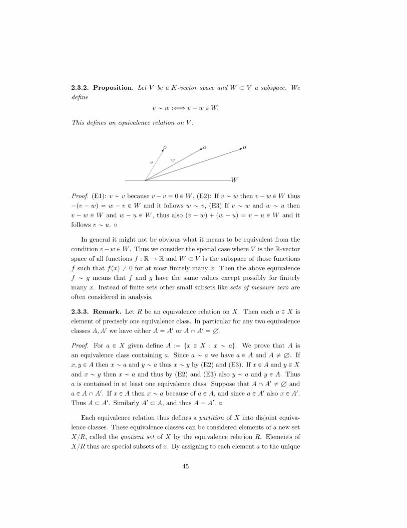
2.3.2. Proposition. Let V be a K-vector space and W Ă V a subspace. We

define

v „ w :ðñ v ´ w PW.

This defines an equivalence relation on V .

o o o-

w

-

v-

W

Proof. (E1): v „ v because v´ v “ 0 PW , (E2): If v „ w then v´w PW thus

´pv ´ wq “ w ´ v P W and it follows w „ v, (E3) If v „ w and w „ u then

v ´ w P W and w ´ u P W , thus also pv ´ wq ` pw ´ uq “ v ´ u P W and it

follows v „ u. ˝

In general it might not be obvious what it means to be equivalent from the

condition v´w PW . Thus we consider the special case where V is the R-vector

space of all functions f : RÑ R and W Ă V is the subspace of those functions

f such that fpxq ‰ 0 for at most finitely many x. Then the above equivalence

f „ g means that f and g have the same values except possibly for finitely

many x. Instead of finite sets other small subsets like sets of measure zero are

often considered in analysis.

2.3.3. Remark. Let R be an equivalence relation on X. Then each a P X is

element of precisely one equivalence class. In particular for any two equivalence

classes A,A1 we have either A “ A1 or AXA1 “ H.

Proof. For a P X given define A :“ tx P X : x „ au. We prove that A is

an equivalence class containing a. Since a „ a we have a P A and A ‰ H. If

x, y P A then x „ a and y „ a thus x „ y by (E2) and (E3). If x P A and y P X

and x „ y then x „ a and thus by (E2) and (E3) also y „ a and y P A. Thus

a is contained in at least one equivalence class. Suppose that AX A1 ‰ H and

a P AX A1. If x P A then x „ a because of a P A, and since a P A1 also x P A1.

Thus A Ă A1. Similarly A1 Ă A, and thus A “ A1. ˝

Each equivalence relation thus defines a partition of X into disjoint equiva-

lence classes. These equivalence classes can be considered elements of a new set

X{R, called the quotient set of X by the equivalence relation R. Elements of

X{R thus are special subsets of x. By assigning to each element a to the unique

45

equivalence class ras containing a there is defined a natural map

X Ñ X{R, a ÞÑ ras.

The preimage set of each A P X{R thus is the set A but now considered as a

subset of X. Each a P A is called representative of the equivalence class A.

We consider the equivalence relation from 2.3.2 and write suggestively V {W

for the quotient set V {R. If v P V we define

v `W :“ tu P V : there is w PW such that u “ v ` wu

and claim this is the equivalence class of v for the given equivalence relation. In

fact, if u P V then u „ v ðñ u´v PW ðñ there is w PW such that u “ v`w.

2.3.4. Example. If V “ K2 and W is a line through the origin then each set

v `W is a line through v. The equivalence classes thus are lines parallel to W

through v.

v `W

o

v

-

W

0

2.3.5. Theorem. Let V be a K-vector space and W Ă V a subspace. Then

there is a unique vector space structure on the set V {W such that the natural

map

ρ : V Ñ V {W, v ÞÑ v `W

is linear. Furthermore:

1. kerρ “W

2. imρ “ V {W

3. dimV {W “ dimV ´ dimW , if dimV ă 8.

Proof. Suppose v, w P V . Then, because we assume

v `W “ ρpvq, w `W “ ρpwq, pv ` wq `W “ ρpv ` wq

it follows from ρpv ` wq “ ρpvq ` ρpwq that

pv `W q ` pw `W q “ pv ` wq `W.

46

(Note that in this equation ` appears with three different meanings!) Similarly

for λ P K it follows that

λ ¨ pv `W q “ λ ¨ v `W.

This proves that our assumption that ρ becomes a linear transformation re-

quires the above definitions of ` and ¨ for the addition and multiplication

by scalars on V {W . It is necessary to show that these definitions are well-

defined, i. e. the definitions do not depend on the choices of representatives, and

pV {W,`, ¨q actually becomes a vector space in this way. First we show that the

two composition operations are well-defined: Let v1w1 be other representatives,

so v `W “ v1 `W and w `W “ w1 `W . Then v ´ v1 P W and w ´ w1 P W

and thus pv ` wq ´ pv1 ` w1q PW and thus

pv ` wq `W “ pv1 ` w1q `W.

(Note that in general a`W “ b`W ðñ a´b PW . ùñ: a`w “ b`w1 implies

a´b “ w1´w PW , ðù: Suppose v P a`W and thus v “ a`w for w PW Since

a´ b PW there is w1 PW such that a “ b`w1 thus v “ b` pw1 `wq P b`W .)

Furthermore λpv ´ v1q PW and thus

λv `W “ λv1 `W,

and multiplication by scalars is also well-defined. Now we need to check the

vector space axioms: The null vector is the equivalence class of 0 and thus

0`W “W “ w`W for all w PW . The negative vector to v`W is p´vq`W .

Checking the remaining vector space axioms is left to the reader. Linearity of ρ

holds by definition. The remaining claims are easy: 1. w P kerρðñ w `W “

0`W ðñ w PW , 2. The natural map onto a quotient set is always surjective,

3. follows from 1. and 2. and the dimension formula. ˝

2.4 Matrices and Linear transformations

We now establish the precise relation between linear transformations and ma-

trices.

Recall from 2.1.4 that given a family B “ pv1, . . . , vnq of vectors of V there

is a uniquely defined linear transformation:

ΦB : Kn Ñ V, px1, . . . , xnq ÞÑ x1v1 ` . . .` xnvn

47

This linear transformation is an isomorphism if and only if B is a basis of V . In

this case, ΦB is called a coordinate system in V . For v P V the vector

x “ px1, . . . , xnq :“ Φ´1B pvq P Kn

is called the coordinate vector of v with respect to the coordinate system ΦB or

shorter B. By definition:

v “ x1v1 ` . . .` xnvn.

Let V,W be K-vector spaces of dimension n respectively m with bases Arespectively B. We will define an isomorphism

LAB : Mpmˆ n;Kq Ñ LKpV,W q, A ÞÑ LA

B pAq “: F

Let A “ pv1, . . . , vnq and B “ pw1, . . . , wmq. Then for a matrix A “ paijqij P

Mpmˆ n;Kq define a linear transformation F : V ÑW by

p˚q F pvjq :“mÿ

i“1

aijwi “ a1jw1 ` . . .` amjwm for j “ 1, . . . n

Because of 2.1.4 this linear transformation is uniquely determined.

Let V “ Kn and W “ Km and let K and K1 be the natural bases. Then

the transformation LKK1 is defined as follows: Write the vectors of Kn and Km

as column vectors, so

x “

¨

˚

˚

˝

x1

...

xn

˛

‹

‹

‚

P Kn and y “

¨

˚

˚

˝

y1

...

ym

˛

‹

‹

‚

P Km.

If A P Mpm ˆ n;Kq then F “ LKK1pAq is given by F pxq “ A ¨ x where A ¨ x is

matrix product as defined in 1.3: y “ A ¨ x is an m ˆ 1-matrix, so a column

vector in Km. Explicitly:¨

˚

˚

˝

a11 . . . a1n

......

am1 . . . amn

˛

‹

‹

‚

¨

˚

˚

˝

x1

...

xn

˛

‹

‹

‚

“

¨

˚

˚

˝

a11x1 ` . . .` a1nxn...

am1x1 ` . . .` amnxn

˛

‹

‹

‚

“

¨

˚

˚

˝

y1

...

ym

˛

‹

‹

‚

In order to see that this coincides with the definition of LKK1 just substitute the

canonical basis vectors e1, . . . , en of Kn (as column vectors) and with the basis

pe11, . . . , e1mq of Km we get

F pejq “ A ¨ ej “

¨

˚

˚

˝

a1j

...

amj

˛

‹

‹

‚

“ a1je11 ` . . .` amje

1m

48

Briefly:

The column vectors of the matrix A are the images of the basis vectors.

Here is a simple example: If A “

˜

1 1

1 ´1

¸

P Mp2 ˆ 2;Kq then F “ LKKpAq is

defined by

F px1, x2q “ px1 ` x2, x1 ´ x2q,

so F pe1q “ F p1, 0q “ p1, 1q and F pe2q “ p1,´1q.

The general case can be reduced to this special case using coordinate systems.

Let V and W be given with bases A and B. Then by the definition of LKK1 for

each A P Mpmˆ n;Kq the following diagram is commutative:

KnLK

K1 pAqÝÝÝÝÝÑ Km

ΦA

§

§

đ

§

§

đ

ΦB

V ÝÝÝÝÑLA

B pAqW

Here a diagram of sets and maps is called commutative if the following

holds: If X,Y are two sets in the diagram and if f, g are two maps resulting

by compositions of maps of the diagram then f “ gsuch that their starting end

end sets coincide. In the diagram above there are only two ways with the same

set in the beginning and end, from Kn to W . Commutativity of the diagram

thus is equivalent to

LAB pAq ˝ ΦA “ ΦB ˝ L

KK1pAq

This can easily be checked from the definitions by evaluation on the basis vectors

ej of K for j “ 1, . . . n, keeping the notation for the other bases as before.

LAB pAq ˝ ΦApejq “ LA

B pAqpvjq “mÿ

i“1

aijwi

and

ΦB ˝ LKK1pAqpejq “ ΦBp

mÿ

i“1

aije1iq “

mÿ

i“1

aijΦBpe1iq “

mÿ

i“1

aijwi.

Now LAB pAq is called the linear transformation V Ñ W associated to the

matrix A with respect to the bases A and B. If V “ W and A “ B we write

shorter LB instead of LAB .

We now describe the matrix associated to a linear transformation. For K-

vector spaces V and W of dimension n respectively m with bases A respectively

49

B define another map

MAB : LKpV,W q ÑMpmˆ n;Kq.

Let F : V Ñ W be linear and A “ pv1, . . . , vnq and B “ pw1, . . . , wmq then

there are for j “ 1, . . . , n uniquely determined a1j , a2j , . . . , amj P K such that

p˚˚q F pvjq “mÿ

i“1

aijwi for j “ 1, . . . n

Then we can define MAB pF q :“ paijqij . Briefly: The column vectors of MA

B pF q

are the coordinate vectors of the images of the basis vectors v1, . . . , vn. Let

v P V , x “

¨

˚

˚

˝

x1

...

xn

˛

‹

‹

‚

P Kn the coordinate vector of v and y “

¨

˚

˚

˝

y1

...

ym

˛

‹

‹

‚

P Km the

coordinate vector of F pvq PW , then

y “MAB pF q ¨ x.

MAB pF q is called the matrix associated to the linear transformation F with

respect to bases A and B, or the matrix representing the linear transformation

with respect to those bases. If V “W and A “ B we write briefly MB for MAB .

2.4.1. Theorem. Let V,W be K-vector spaces, dimV “ n and dimW “ m.

Let A “ pv1, . . . , vnq a basis of V and let B “ pw1, . . . , wmq be a basis of W .

Then the map

LAB : Mpmˆ n;Kq Ñ LKpV,W q, A ÞÑ LA

B pAq

is a vector space isomorphism with inverse defined by

MAB : LKpV,W q Ñ Mpmˆ n;Kq, F ÞÑMA

B pF q

Proof. We abbreviate L and M for LAB and MA

B . Let A,B P Mpmˆ n;Kq and

λ, µ P K. We claim that

LpλA` µBq “ λLpAq ` µLpBq.

For this we use the coordinate systems

ΦA : Kn Ñ V, and ΦB : Km ÑW.

Let v P V and x “ Φ´1A pvq the corresponding coordinate vector. Then

LpλA` µBqpvq “ ΦBppλA` µBqxq “

50

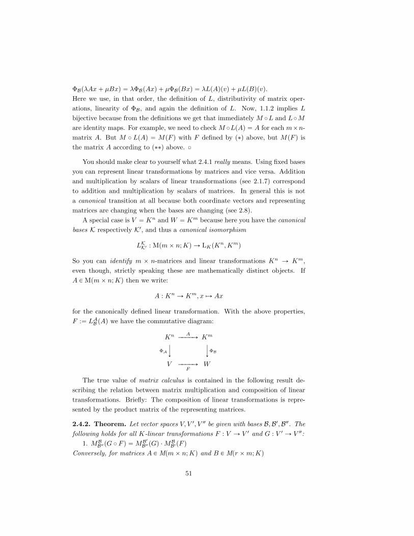
ΦBpλAx` µBxq “ λΦBpAxq ` µΦBpBxq “ λLpAqpvq ` µLpBqpvq.

Here we use, in that order, the definition of L, distributivity of matrix oper-

ations, linearity of ΦB, and again the definition of L. Now, 1.1.2 implies L

bijective because from the definitions we get that immediately M ˝L and L˝M

are identity maps. For example, we need to check M ˝LpAq “ A for each mˆn-

matrix A. But M ˝ LpAq “ MpF q with F defined by p˚q above, but MpF q is

the matrix A according to p˚˚q above. ˝

You should make clear to yourself what 2.4.1 really means. Using fixed bases

you can represent linear transformations by matrices and vice versa. Addition

and multiplication by scalars of linear transformations (see 2.1.7) correspond

to addition and multiplication by scalars of matrices. In general this is not

a canonical transition at all because both coordinate vectors and representing

matrices are changing when the bases are changing (see 2.8).

A special case is V “ Kn and W “ Km because here you have the canonical

bases K respectively K1, and thus a canonical isomorphism

LKK1 : Mpmˆ n;Kq Ñ LKpK

n,Kmq

So you can identify m ˆ n-matrices and linear transformations Kn Ñ Km,

even though, strictly speaking these are mathematically distinct objects. If

A P Mpmˆ n;Kq then we write:

A : Kn Ñ Km, x ÞÑ Ax

for the canonically defined linear transformation. With the above properties,

F :“ LAB pAq we have the commutative diagram:

Kn AÝÝÝÝÑ Km

ΦA

§

§

đ

§

§

đ

ΦB

V ÝÝÝÝÑF

W

The true value of matrix calculus is contained in the following result de-

scribing the relation between matrix multiplication and composition of linear

transformations. Briefly: The composition of linear transformations is repre-

sented by the product matrix of the representing matrices.

2.4.2. Theorem. Let vector spaces V, V 1, V 2 be given with bases B,B1,B2. The

following holds for all K-linear transformations F : V Ñ V 1 and G : V 1 Ñ V 2:

1. MBB2pG ˝ F q “MB1

B2pGq ¨MBB1pF q

Conversely, for matrices A P Mpmˆ n;Kq and B P Mpr ˆm;Kq

51

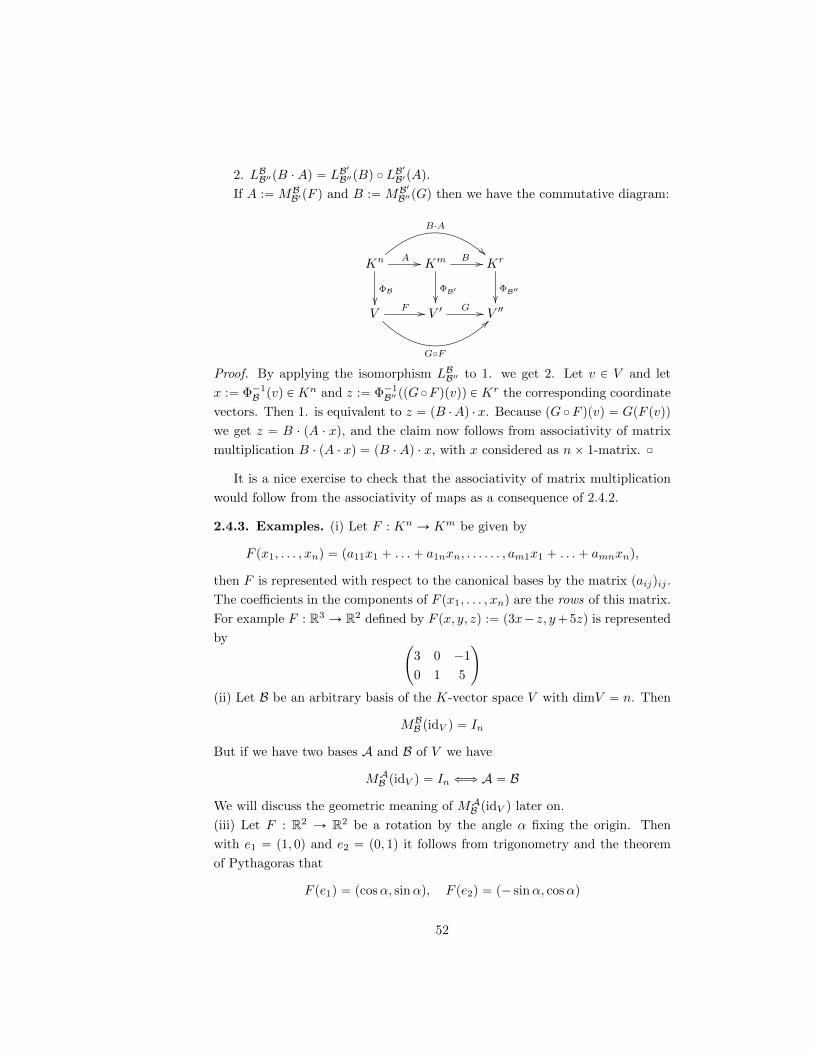
2. LBB2pB Äq “ LB1

B2pBq ˝ LB1B1pAq.

If A :“MBB1pF q and B :“MB1

B2pGq then we have the commutative diagram:

Kn

BÄ

!!

ΦB

��

A // Km

ΦB1��

B // Kr

ΦB2��

V

G˝F

>>F // V 1

G // V 2

Proof. By applying the isomorphism LBB2 to 1. we get 2. Let v P V and let

x :“ Φ´1B pvq P Kn and z :“ Φ´1

B2 ppG˝F qpvqq P Kr the corresponding coordinate

vectors. Then 1. is equivalent to z “ pB Äq ¨ x. Because pG ˝F qpvq “ GpF pvqq

we get z “ B ¨ pA ¨ xq, and the claim now follows from associativity of matrix

multiplication B ¨ pA ¨ xq “ pB Äq ¨ x, with x considered as nˆ 1-matrix. ˝

It is a nice exercise to check that the associativity of matrix multiplication

would follow from the associativity of maps as a consequence of 2.4.2.

2.4.3. Examples. (i) Let F : Kn Ñ Km be given by

F px1, . . . , xnq “ pa11x1 ` . . .` a1nxn, . . . . . . , am1x1 ` . . .` amnxnq,

then F is represented with respect to the canonical bases by the matrix paijqij .

The coefficients in the components of F px1, . . . , xnq are the rows of this matrix.

For example F : R3 Ñ R2 defined by F px, y, zq :“ p3x´z, y`5zq is represented

by˜

3 0 ´1

0 1 5

¸

(ii) Let B be an arbitrary basis of the K-vector space V with dimV “ n. Then

MBB pidV q “ In

But if we have two bases A and B of V we have

MAB pidV q “ In ðñ A “ B

We will discuss the geometric meaning of MAB pidV q later on.

(iii) Let F : R2 Ñ R2 be a rotation by the angle α fixing the origin. Then

with e1 “ p1, 0q and e2 “ p0, 1q it follows from trigonometry and the theorem

of Pythagoras that

F pe1q “ pcosα, sinαq, F pe2q “ p´ sinα, cosαq

52

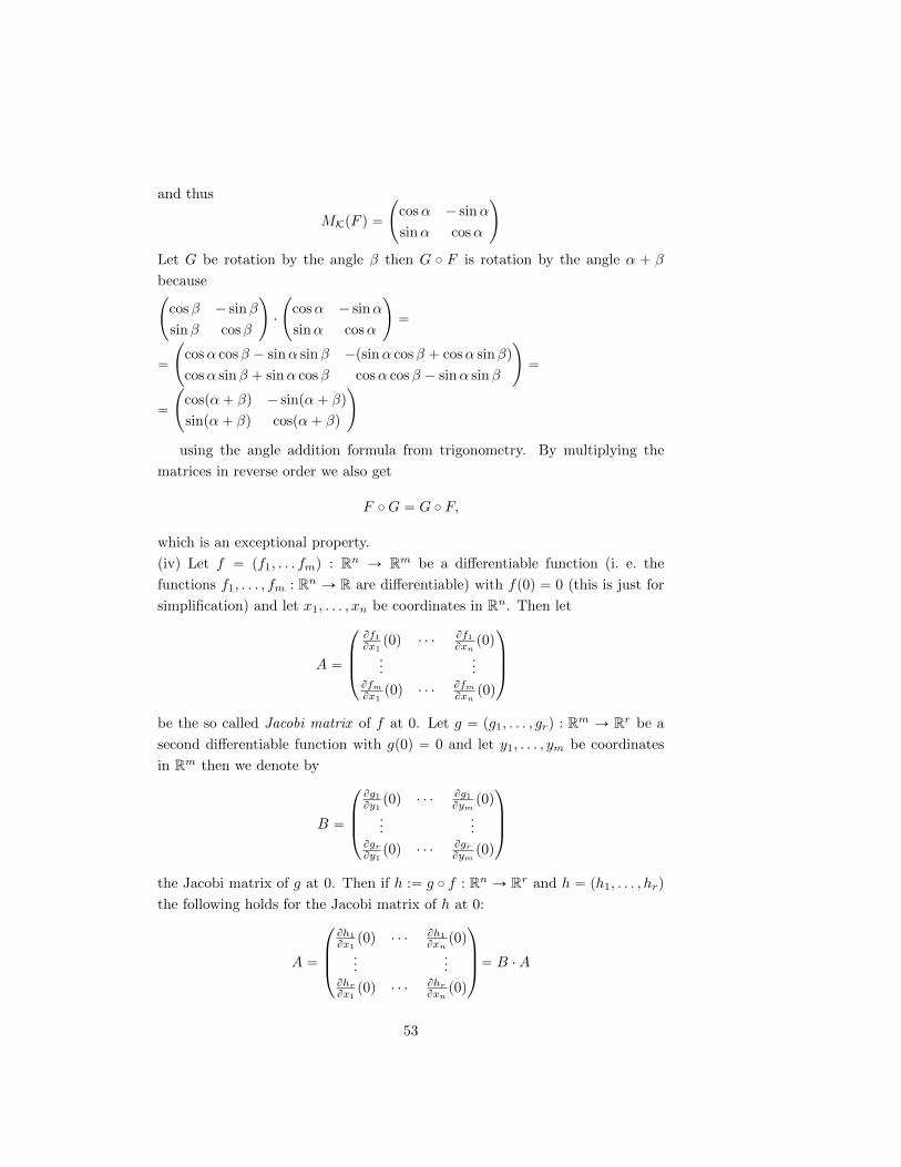
and thus

MKpF q “

˜

cosα ´ sinα

sinα cosα

¸

Let G be rotation by the angle β then G ˝ F is rotation by the angle α ` β

because˜

cosβ ´ sinβ

sinβ cosβ

¸

¨

˜

cosα ´ sinα

sinα cosα

¸

“

“

˜

cosα cosβ ´ sinα sinβ ´psinα cosβ ` cosα sinβq

cosα sinβ ` sinα cosβ cosα cosβ ´ sinα sinβ

¸

“

“

˜

cospα` βq ´ sinpα` βq

sinpα` βq cospα` βq

¸

using the angle addition formula from trigonometry. By multiplying the

matrices in reverse order we also get

F ˝G “ G ˝ F,

which is an exceptional property.

(iv) Let f “ pf1, . . . fmq : Rn Ñ Rm be a differentiable function (i. e. the

functions f1, . . . , fm : Rn Ñ R are differentiable) with fp0q “ 0 (this is just for

simplification) and let x1, . . . , xn be coordinates in Rn. Then let

A “

¨

˚

˚

˝

Bf1Bx1p0q ¨ ¨ ¨

Bf1Bxnp0q

......

BfmBx1p0q ¨ ¨ ¨

BfmBxnp0q

˛

‹

‹

‚

be the so called Jacobi matrix of f at 0. Let g “ pg1, . . . , grq : Rm Ñ Rr be a

second differentiable function with gp0q “ 0 and let y1, . . . , ym be coordinates

in Rm then we denote by

B “

¨

˚

˚

˝

Bg1By1p0q ¨ ¨ ¨

Bg1Bym

p0q...

...BgrBy1p0q ¨ ¨ ¨

BgrBym

p0q

˛

‹

‹

‚

the Jacobi matrix of g at 0. Then if h :“ g ˝ f : Rn Ñ Rr and h “ ph1, . . . , hrq

the following holds for the Jacobi matrix of h at 0:

A “

¨

˚

˚

˝

Bh1

Bx1p0q ¨ ¨ ¨ Bh1

Bxnp0q

......

BhrBx1p0q ¨ ¨ ¨ Bhr

Bxnp0q

˛

‹

‹

‚

“ B ¨A

53

This follows from the rules of partial differentiation. Historically this kind of

relation between systems of partial derivatives has been the starting point for

the development of matrix calculus.

2.5 Calculating with matrices

We assume that K is a field. Let A be an m ˆ n-matrix. An elementary row

operation of A is defined by one of the following:

(I) Multiplication of the i-th row by λ P K˚:

A “

¨

˚

˚

˚

˝

...

ai...

˛

‹

‹

‹

‚

ÞÑ

¨

˚

˚

˚

˝

...

λai...

˛

‹

‹

‹

‚

“: AI

(II) Addition of the j-th row to the i-th row:

A “

¨

˚

˚

˚

˚

˚

˚

˚

˚

˝

...

ai...

aj...

˛

‹

‹

‹

‹

‹

‹

‹

‹

‚

ÞÑ

¨

˚

˚

˚

˚

˚

˚

˚

˚

˝

...

ai ` aj...

aj...

˛

‹

‹

‹

‹

‹

‹

‹

‹

‚

“: AII

(III) Addition of the λ-multiple of the j-th row to the i-th row for λ P K˚:

A “

¨

˚

˚

˚

˚

˚

˚

˚

˚

˝

...

ai...

aj...

˛

‹

‹

‹

‹

‹

‹

‹

‹

‚

ÞÑ

¨

˚

˚

˚

˚

˚

˚

˚

˚

˝

...

ai ` λaj...

aj...

˛

‹

‹

‹

‹

‹

‹

‹

‹

‚

“: AIII

(IV) Exchange the i-th row and the j-th row (i ‰ j):

A “

¨

˚

˚

˚

˚

˚

˚

˚

˚

˝

...

ai...

aj...

˛

‹

‹

‹

‹

‹

‹

‹

‹

‚

ÞÑ

¨

˚

˚

˚

˚

˚

˚

˚

˚

˝

...

aj...

ai...

˛

‹

‹

‹

‹

‹

‹

‹

‹

‚

“: AIV

54

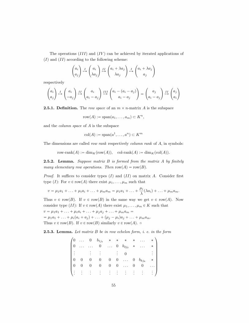
The operations (III) and (IV ) can be achieved by iterated applications of

(I) and (II) according to the following scheme:˜

ai

aj

¸

IÞÑ

˜

ai

λaj

¸

IIÞÑ

˜

ai ` λaj

λaj

¸

IÞÑ

˜

ai ` λaj

aj

¸

respectively˜

ai

aj

¸

IÞÑ

˜

ai

´aj

¸

IIÞÑ

˜

ai

ai ´ aj

¸

IIIÞÑ

˜

ai ´ pai ´ ajq

ai ´ aj

¸

“

˜

aj

ai ´ aj

¸

IIÞÑ

˜

aj

ai

¸

2.5.1. Definition. The row space of an mˆ n-matrix A is the subspace

rowpAq :“ spanpa1, . . . , amq Ă Kn,

and the column space of A is the subspace

colpAq :“ spanpa1, . . . , anq Ă Km

The dimensions are called row rank respectively column rank of A, in symbols:

row-rankpAq :“ dimKprowpAqq, col-rankpAq :“ dimKpcolpAqq.

2.5.2. Lemma. Suppose matrix B is formed from the matrix A by finitely

many elementary row operations. Then rowpAq “ rowpBq.

Proof. It suffices to consider types (I) and (II) on matrix A. Consider first

type (I): For v P rowpAq there exist µ1, . . . , µm such that

v “ µ1a1 ` . . .` µiai ` . . .` µmam “ µ1a1 ` . . .`µiλpλaiq ` . . .` µmam.

Thus v P rowpBq. If v P rowpBq in the same way we get v P rowpAq. Now

consider type (II): If v P rowpAq there exist µ1, . . . , µm P K such that

v “ µ1a1 ` . . .` µiai ` . . .` µjaj ` . . .` µmam “

“ µ1a1 ` . . .` µipai ` ajq ` . . .` pµj ´ µiqaj ` . . .` µmam.

Thus v P rowpBq. If v P rowpBq similarly v P rowpAq. ˝

2.5.3. Lemma. Let matrix B be in row echelon form, i. e. in the form¨

˚

˚

˚

˚

˚

˚

˚

˚

˚

˚

˝

0 . . . 0 b1j1 ˚ ˚ ˚ ˚ . . . ˚

0 . . . . . . 0 . . . 0 b2j2 ˚ . . . ˚

......

...... 0

...

0 0 0 0 0 0 . . . 0 bkjk ˚

0 0 0 0 0 0 . . . 0 0 . . ....

......

......

......

......

...

˛

‹

‹

‹

‹

‹

‹

‹

‹

‹

‹

‚

55

with all components b1j1 , . . . , bkjk ‰ 0, the other components above the stairs

arbitrary and all components under the stairs 0. Then if b1, . . . , bk are the first k

row vectors of B, pb1, . . . , bkq is a basis of rowpBq. In particular row-rankpAq “

k.

Proof. It suffices to show that b1, . . . , bk are linearly independent because the

remaining rows are 0. If for λ1, . . . , λk P K we have

λ1b1 ` . . .` λkbk “ 0,

then in particular for the j1 components

λ1b1j1 “ 0,

and so λ1 “ 0 since b1j1 ‰ 0. Thus

λ2b2 ` . . .` λkbk “ 0

which implies similarly λ2 “ 0 and so on until finally λk “ 0. ˝

2.5.4. Lemma. Each m ˆ n-matrix A can be transformed into row echelon

form using finitely many row operations of type III and IV.

Writing up the detailed proof requires lots of notation and in particular is

incredibly boring. See the following link:

http://algebra.math.ust.hk/linear_equation/04_echelon_form/lecture3.

shtml

for an example, which shows all important features of the general case. The

proof proceeds is by induction. It starts with the selection of a pivot element

(the first non-zero element found by scanning through the columns starting from

the left and top), which is brought to the first row by a type IV operation. Then

all the other elements in the corresponding column can be eliminated (i. e. be

made 0) by type III operations. In the next step the process is applied to the

sub-matrix defined from the original matrix by deleting the first row and the

zero-columns to the left of the pivot element.

Using 2.5.3 and 2.5.4 we now have a practical method to find for v1, . . . , vm P

Kn a basis of spanpv1, . . . , vmq. Form the matrix with rows the given vectors,

transform into row echelon form. The non-zero vectors are vectors of a basis.

For a square matrix A “ paijq1ďi,jďn the diagonal entries are the entries aii

for i “ 1, . . . , n.

2.5.5. Corollary. For vectors v1, . . . , vn P Kn the following are equivalent:

(i) pv1, . . . , vnq is a basis of Kn.

56

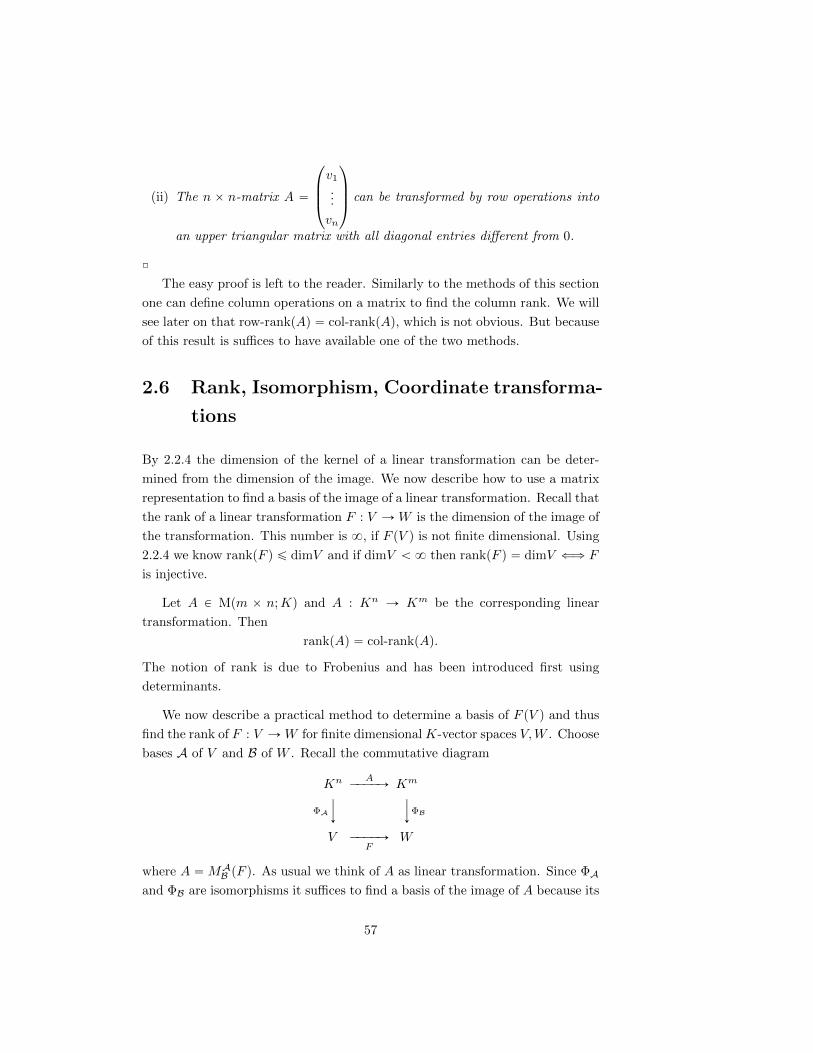
http://algebra.math.ust.hk/linear_equation/04_echelon_form/lecture3.shtml

http://algebra.math.ust.hk/linear_equation/04_echelon_form/lecture3.shtml

(ii) The n ˆ n-matrix A “

¨

˚

˚

˝

v1

...

vn

˛

‹

‹

‚

can be transformed by row operations into

an upper triangular matrix with all diagonal entries different from 0.

˝

The easy proof is left to the reader. Similarly to the methods of this section

one can define column operations on a matrix to find the column rank. We will

see later on that row-rankpAq “ col-rankpAq, which is not obvious. But because

of this result is suffices to have available one of the two methods.

2.6 Rank, Isomorphism, Coordinate transforma-

tions

By 2.2.4 the dimension of the kernel of a linear transformation can be deter-

mined from the dimension of the image. We now describe how to use a matrix

representation to find a basis of the image of a linear transformation. Recall that

the rank of a linear transformation F : V ÑW is the dimension of the image of

the transformation. This number is 8, if F pV q is not finite dimensional. Using

2.2.4 we know rankpF q ď dimV and if dimV ă 8 then rankpF q “ dimV ðñ F

is injective.

Let A P Mpm ˆ n;Kq and A : Kn Ñ Km be the corresponding linear

transformation. Then

rankpAq “ col-rankpAq.

The notion of rank is due to Frobenius and has been introduced first using

determinants.

We now describe a practical method to determine a basis of F pV q and thus

find the rank of F : V ÑW for finite dimensional K-vector spaces V,W . Choose

bases A of V and B of W . Recall the commutative diagram

Kn AÝÝÝÝÑ Km

ΦA

§

§

đ

§

§

đ

ΦB

V ÝÝÝÝÑF

W

where A “MAB pF q. As usual we think of A as linear transformation. Since ΦA

and ΦB are isomorphisms it suffices to find a basis of the image of A because its

57

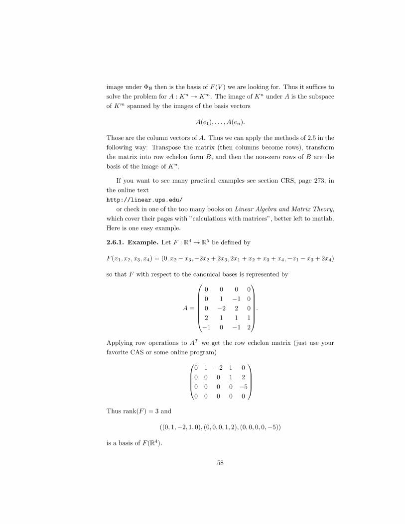
image under ΦB then is the basis of F pV q we are looking for. Thus it suffices to

solve the problem for A : Kn Ñ Km. The image of Kn under A is the subspace

of Km spanned by the images of the basis vectors

Ape1q, . . . , Apenq.

Those are the column vectors of A. Thus we can apply the methods of 2.5 in the

following way: Transpose the matrix (then columns become rows), transform

the matrix into row echelon form B, and then the non-zero rows of B are the

basis of the image of Kn.

If you want to see many practical examples see section CRS, page 273, in

the online text

http://linear.ups.edu/

or check in one of the too many books on Linear Algebra and Matrix Theory,

which cover their pages with ”calculations with matrices”, better left to matlab.

Here is one easy example.

2.6.1. Example. Let F : R4 Ñ R5 be defined by

F px1, x2, x3, x4q “ p0, x2 ´ x3,´2x2 ` 2x3, 2x1 ` x2 ` x3 ` x4,´x1 ´ x3 ` 2x4q

so that F with respect to the canonical bases is represented by

A “

¨

˚

˚

˚

˚

˚

˚

˝

0 0 0 0

0 1 ´1 0

0 ´2 2 0

2 1 1 1

´1 0 ´1 2

˛

‹

‹

‹

‹

‹

‹

‚

.

Applying row operations to AT we get the row echelon matrix (just use your

favorite CAS or some online program)

¨

˚

˚

˚

˝

0 1 ´2 1 0

0 0 0 1 2

0 0 0 0 ´5

0 0 0 0 0

˛

‹

‹

‹

‚

Thus rankpF q “ 3 and

pp0, 1,´2, 1, 0q, p0, 0, 0, 1, 2q, p0, 0, 0, 0,´5qq

is a basis of F pR4q.

58


Because computers are much better in calculating than human beings (who

are still better in proving theorems..) we return to more theoretical concepts

concerning the relation between linear transformations and matrices.

Particularly interesting linear transformations F : V Ñ W are the isomor-

phisms, for which rankpF q “ dimV “ dimW .

2.6.2. Lemma. For a linear transformation F : V Ñ W between finite

dimensional vector spaces with dimV “ dimW the following are equivalent:

(i) F is injective.

(ii) F is surjective.

(iii) F is bijective.

Proof. Apply the dimension formula 2.2.4

dimV “ dimW “ dimpimF qq ` dimpkerF qq

and Lemma 2.2.2. ˝

Thus to decide whether a linear transformation is an isomorphism first check

the necessary condition

dimV “ dimW.

Then calculate the rank of F using the above method, and by 2.6.2 the linear

transformation is an isomorphism if rankpF q “ dimW .

2.6.3. Definition. Let R be a commutative unital ring. A square matrix

A P Mpn ˆ n;Rq is invertible (sometimes also called regular) if there exists a

matrix A1 P Mpnˆ n;Rq such that

A ¨A1 “ A1 ¨A “ In

A matrix which is not invertible is also called singular.

2.6.4. Definition and Proposition. The set

GLpn;Rq :“ tA P Mpnˆ n;Rq : A is invertibleu

with the usual multiplication of matrices is a group. It is called the general linear

group.

Proof. Given A,B P GLpn;Rq let A1, B1 be matrices such that

AA1 “ A1A “ In “ BB1 “ B1B.

59

Then

pB1A1qpABq “ B1pA1AqB “ B1InB “ B1B “ In

and

pABqpB1A1q “ ApBB1qA1 “ AInA1 “ AA1 “ In

using associativity of matrix multiplication, thus A,B P GLpn;Rq. We now

show (G1) and (G2) from 1.2.1. Associativity holds in GLpn;Rq because it

holds in Mpn ˆ n;Rq. The neutral element is In, and for each A P GLpn;Rq

there is by definition an inverse A1. ˝

The transposition of matrices Mpm ˆ n;Rq Ñ Mpn ˆ n;Rq is defined just

like in the case of a field. If A “ paijqij then AT :“ pbijqij with bij :“ aji for

all 1 ď i ď m, 1 ď j ď n.

We have seen in 1.2. that the inverse A1 of A P Mpn ˆ n;Rq is uniquely

determined and is denoted A´1. Then

pA´1q´1 “ A, and pABq´1 “ B´1A´1.

If A is invertible then also AT and

pAT q´1 “ pA´1qT

because

pA´1qTAT “ pAA´1qT “ ITn “ In.

Now we come back to linear transformations and matrices with entries in fields.

2.6.5. Theorem. Let F : V Ñ W be a linear transformation, dimV “

dimW “ n ă 8 and let A and B be any two bases of V and W . Then the

following are equivalent:

(i) F is an isomorphism.

(ii) The representing matrix MAB pF q is invertible.

If F is an isomorphism then

MBApF

´1q “ pMAB pF qq

´1,

so the inverse transformation is represented by the inverse matrix.

Proof. Let A :“MAB pF q.

(i) ùñ (ii): Let F be an isomorphism and F´1 the inverse, then we define

A1 :“MBApF

´1q. Because of 2.4.2 we have

A ¨A1 “MBpF ˝ F´1q “MBpidW q “ In and

60

A1 Ä “MApF´1 ˝ F q “MApidV q “ In,

also A P GLpn;Kq. Since A1 “ A´1 also the additional claim follows.

(ii) ùñ (i): If A is invertible we define G :“ LBApA

´1q. Because of 2.4.2 again

we have

F ˝G “ LBpA Ä´1q “ LBpInq “ idW and

G ˝ F “ LApA´1 Äq “ LApInq “ idV

By 1.1.3 it follows that F is bijective. ˝

2.6.6. Corollary. For A P Mpnˆ n;Kq the following are equivalent:

(i) A is invertible.

(ii) AT is invertible.

(iii) col-rankpAq “ n

(iv) row-rankpAq “ n

Proof. (i)ðñ (ii) has been proved after the proof of 2.6.4 and using pAT qT “ A.

(i) ðñ (iii) follows from 2.6.5 and 2.6.2 applied to the linear transformation

A : Kn Ñ Kn. (ii) ðñ (iv) follows from (i) ðñ (iii) by transposition. ˝

We now discuss basis change and coordinate transformation. Let V be a

K-vector space of dimension n and A “ pv1, . . . , vnq be a basis of V and

ΦA : Kn Ñ V, px1, . . . , xnq ÞÑ x1v1 ` . . .` xnvn

be the corresponding coordinate system. If we change to a basis B “ pw1, . . . , wnq

of V then we have a new coordinate system

ΦB : Kn Ñ V, py1, . . . , ynq ÞÑ y1w1 ` . . .` ynwn.

The question is how we find for v P V the new coordinates y “ Φ´1B pvq from

x “ Φ´1A pvq. The passage from x to y is given by the isomorphism

T :“ Φ´1B ˝ ΦA P GLpKnq

making the diagram

Kn T - Kn

V

ΦB�ΦA-

61

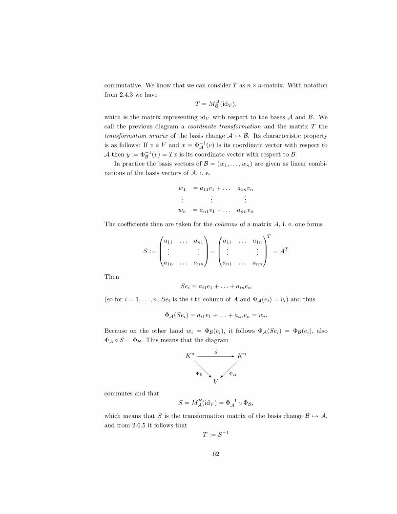
commutative. We know that we can consider T as nˆn-matrix. With notation

from 2.4.3 we have

T “MAB pidV q,

which is the matrix representing idV with respect to the bases A and B. We

call the previous diagram a coordinate transformation and the matrix T the

transformation matrix of the basis change A ÞÑ B. Its characteristic property

is as follows: If v P V and x “ Φ´1A pvq is its coordinate vector with respect to

A then y :“ Φ´1B pvq “ Tx is its coordinate vector with respect to B.

In practice the basis vectors of B “ pw1, . . . , wnq are given as linear combi-

nations of the basis vectors of A, i. e.

w1 “ a11v1 ` . . . a1nvn...

......

wn “ an1v1 ` . . . annvn

The coefficients then are taken for the columns of a matrix A, i. e. one forms

S :“

¨

˚

˚

˝

a11 . . . an1

......

a1n . . . ann

˛

‹

‹

‚

“

¨

˚

˚

˝

a11 . . . a1n

......

an1 . . . ann

˛

‹

‹

‚

T

“ AT

Then

Sei “ ai1e1 ` . . .` ainen

(so for i “ 1, . . . , n, Sei is the i-th column of A and ΦApeiq “ vi) and thus

ΦApSeiq “ ai1v1 ` . . .` ainvn “ wi.

Because on the other hand wi “ ΦBpeiq, it follows ΦApSeiq “ ΦBpeiq, also

ΦA ˝ S “ ΦB. This means that the diagram

Kn S - Kn

V

ΦA�ΦB-

commutes and that

S “MBApidV q “ Φ´1

A ˝ ΦB,

which means that S is the transformation matrix of the basis change B ÞÑ A,

and from 2.6.5 it follows that

T :“ S´1

62

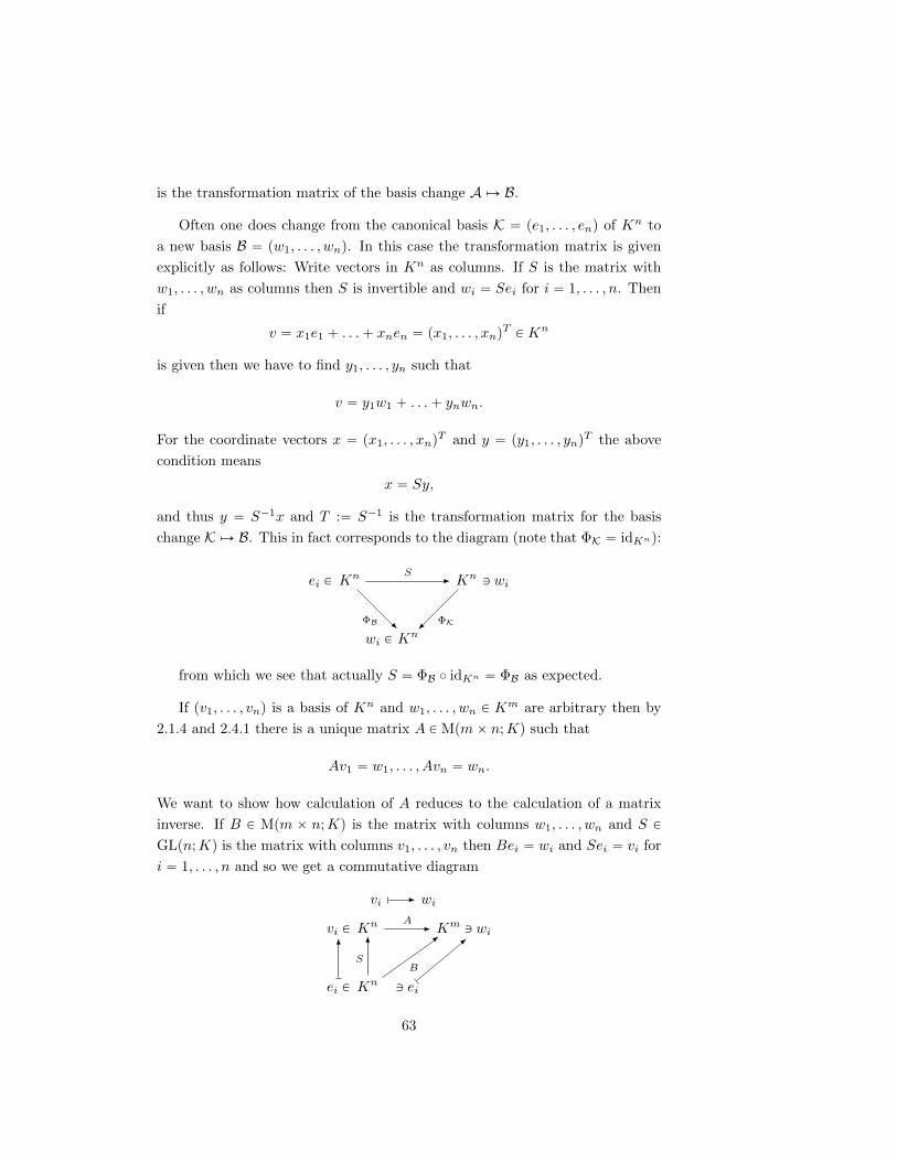
is the transformation matrix of the basis change A ÞÑ B.

Often one does change from the canonical basis K “ pe1, . . . , enq of Kn to

a new basis B “ pw1, . . . , wnq. In this case the transformation matrix is given

explicitly as follows: Write vectors in Kn as columns. If S is the matrix with

w1, . . . , wn as columns then S is invertible and wi “ Sei for i “ 1, . . . , n. Then

if

v “ x1e1 ` . . .` xnen “ px1, . . . , xnqT P Kn

is given then we have to find y1, . . . , yn such that

v “ y1w1 ` . . .` ynwn.

For the coordinate vectors x “ px1, . . . , xnqT and y “ py1, . . . , ynq

T the above

condition means

x “ Sy,

and thus y “ S´1x and T :“ S´1 is the transformation matrix for the basis

change K ÞÑ B. This in fact corresponds to the diagram (note that ΦK “ idKn):

ei P Kn S - Kn Q wi

wi P Kn

ΦK�ΦB-

from which we see that actually S “ ΦB ˝ idKn “ ΦB as expected.

If pv1, . . . , vnq is a basis of Kn and w1, . . . , wn P Km are arbitrary then by

2.1.4 and 2.4.1 there is a unique matrix A P Mpmˆ n;Kq such that

Av1 “ w1, . . . , Avn “ wn.

We want to show how calculation of A reduces to the calculation of a matrix

inverse. If B P Mpm ˆ n;Kq is the matrix with columns w1, . . . , wn and S P

GLpn;Kq is the matrix with columns v1, . . . , vn then Bei “ wi and Sei “ vi for

i “ 1, . . . , n and so we get a commutative diagram

vi - wi

vi P Kn A- Km Q wi

ei P

6

Kn

S6

B

-

Q ei

-

63

of linear transformations.. It follows B “ AS and so A “ BS´1. This can also

be calculated directly: From BS´1vi “ Bei “ wi for i “ 1, . . . , n it follows that

BS´1 “ A.

2.7 Elementary matrices

Let m be a positive integer. Recall that I “ Im is the m ˆm identity matrix,

and from 1.5.18 (vii) the matrices Eji P Mpmˆm;Kq with all entries 0 except

1 in the ij position. For 1 ď i, j ď m, i ‰ j and λ P K˚ define the elementary

matrices

Sipλq :“ I ` pλ´ 1qEii ,

(Thus Sipλq differs from Im only in the ii-position where 1 has been replaced

by λ.)

Qji pλq :“ I ` λEji

and

P ji :“ I ´ Eii ´ Ejj ` E

ji ` E

ij .

We also write Qji :“ Qji p1q. Note that P ji “ P ij . Recall the elementary row

operations from 2.5. We have

AI “ Sipλq Ä, AII “ Qji Ä, AIII “ Qji pλq Ä, AIV “ P ji Ä

If we similarly define elementary column operations by

AI multiplication of i-th colum by λ,

AII addition of j-th column to i-th column,

AIII addition of the λ-multiple of the j-th column to the i-th column,

AIV change of the i-th and the j-th column

we can also write

AI “ A ¨ Sipλq, AII “ A ¨Qji , AIII “ A ¨Qji pλq, AIV “ A ¨ P ij

Briefly: Multiplication from the left by elementary matrices has the effect of ele-

mentary row operations, and multiplication on the right by elementary matrices

has the effect of elementary column operations.

64

Remark. The elementary matrices of type Qji pλq and P ji are products of ele-

mentary matrices of type Sipλq and Qji , more precisely:

Qji pλq “ Sjp1

λq ¨Qji ¨ Sjpλq

P ji “ Qij ¨Qji p´1q ¨Qij ¨ Sjp´1q

This corresponds to the remark from 2.5 that elementary operations of type III

and IV can be combined by those of type I and II.

2.7.1. Lemma. Elementary matrices are invertible and inverses are elemen-

tary matrices, more precisely:

pSipλqq´1 “ Sip

1

λq, pQji q

´1 “ Qji p´1q, pQji pλqq´1 “ Qji p´λq, pP ji q

´1 “ P ji

Proof. Just multiply the matrices on the right hand side with those on the left

hand side to see that you get identity matrices. ˝

A square matrix A “ paijqij is called an upper triangular respectively lower

triangular matrix if aij “ 0 for i ą j respectively i ă j.

2.7.2. Theorem. Each invertible matrix A P Mpn ˆ n;Kq is a product of

elementary matrices, i. e. the group GLpn;Kq is generated by the elementary

matrices.

Proof. By 2.6.6 the row rank of A is n. As we saw in 2.5 the matrix A can be

transformed into the upper triangular matrix

B “

¨

˚

˚

˝

b11 . . . b1n...

. . ....

0 . . . bnn

˛

‹

‹

‚

with bii ‰ 0 for all 1 ď i ď n. By the above there are elementary matrices

B1, . . . , Br such that

B “ Br ¨Br´1 ¨ . . . ¨B1 ¨A

Using further row operations the matrix can be transformed into the iden-

tity matrix In. For this use the last row to eliminate b1n, . . . , bn´1,n, then

b1,n´1, . . . , bn´2,n´1 using the pn´ 1q-st row and so on. Finally the components

on the diagonal can be normalized. So by the above there are further elementary

matrices Br`1, . . . , Bs such that

In “ Bs ¨ . . . Br`1 ¨B “ Bs ¨ . . . ¨B1 ¨A

65

From this we deduce

A´1 “ Bs ¨ . . . ¨B1, thus A “ B´11 ¨ . . . ¨B´1

s ,

and the claim follows from 2.7.1. ˝

2.7.3. Definition. Let R be a commutative unital ring. A matrix A is called

a diagonal matrix if aij “ 0 for i ‰ j. For each vector d P Rn we denote by

diagpdq the diagonal matrix

diagpdq :“

¨

˚

˚

˝

d1 0 . . . 0...

. . ....

0 . . . dn

˛

‹

‹

‚

2.7.4. Remark. Note that if A “ paijqij P Mpnˆ n;Rq and d “ pd1, . . . , dnq P

Rn then

diagpdq ¨A “

¨

˚

˚

˚

˚

˝

d1a11 d1a12 . . . d1a1n

d2a21 d2a22 . . . d2a2n

......

dnan1 dnan2 . . . dnann

˛

‹

‹

‹

‹

‚

and

A ¨ diagpdq “

¨

˚

˚

˚

˚

˝

d1a11 d2a12 . . . dna1n

d1a21 d2a22 . . . dna2n

......

d1an1 d2an2 . . . dnann

˛

‹

‹

‹

‹

‚

Thus if diagpdq is invertible then there exist aii P R such that diaii “ aiidi “

1 and thus the diagonal elements are units of the ring, i. e. di P Rˆ. Conversely,

each diagonal matrix diagpdq with all di P Rˆ is invertible with inverse matrix

diagpd1q where d1 :“ pd´11 , . . . , d´1

n q. A notion of elementary matrices over R

is easily defined by restricting parameters for the matrices Sipλq to units, i. e.

λ P Rˆ. But the question when GLpn;Rq is generated by elementary matrices is

subtle because of Lemma 2.5.4, which does not hold over arbitrary commutative

unital rings. The problem is to find the pivot elements of the column vectors

in Rˆ, which are necessary to achieve, possibly after permutation of rows, the

upper triangular form. This requires a euclidean algorithm, and even though

the result does not always work it works in some important cases like R “ Z.

2.7.5. Remark. The proof of 2.7.2 also gives a practical method to find the

inverse of a given matrix. This method in particular does not even require a

66

priori knowledge of whether the matrix to start with is invertible. In fact, given

an nˆn-matrix A form the extended nˆ2n-matrix pA, Inq. Now one first starts

with row operations on A to see whether the row rank is n. If not then one

stops. Otherwise one performs the very same row operations on the matrix In

too. Then one keeps on going with row operations until the matrix A has been

transformed into the identity matrix

pA, Inq ÞÑ pBs ¨ . . . ¨B1 Ä,Bs ¨ . . . ¨B1q “ pIn, Bs ¨ . . . ¨B1q.

Then from Bs ¨ . . . ¨B1 Ä “ In it follows that Bs ¨ . . . ¨B1 Ïn “ Bs ¨ . . . ¨B1 “ A´1.

Instead of row operations one can also use exclusively column operations.

But the method will not work in general if we use both row and column opera-

tions.

For some explicit examples see Example 159-161, page 56 in

http://faculty.ccp.edu/dept/math/251-linear-algebra/santos-notes.pdf.

The first of the examples at the link above is for the field K “ Z7. In general,

we define for n a positive integer a commutative unital ring Zn as follows:

Consider the set of numbers t0, 1, . . . , n ´ 1u and define addition respectively

multiplication of two numbers by adding respectively multiplying the numbers

in the usual sense and then taking the remainder in t0, 1 . . . , n´ 1u for division

by n. If we denote the remainder of an integer a in this way by a “ a modpnq

we define a ` b :“ a` b and a ¨ b :“ ab. (a is the equivalence class of a P Zunder the equivalence relation on Z defined by a „ bðñ a´b is divisible by n.)

The ring axioms are easily checked and 1 is the neutral element with respect to

multiplication. If n “ p is a prime number this is the field Zp. In fact because

gcdpa, pq “ 1 for 1 ď a ď p´ 1 we can find integers x, y such that ax` bp “ 1

and thus ax´ 1 is divisible by p (Euclidean algorithm). Then the remainder of

x modppq is the multiplicative inverse of a.

2.8 Rank and equivalence of matrices

In this section we begin with the question whether by a choice of a special basis

we can find a particularly simple matrix representation.

Let F : V ÑW be a linear transformation of K-vector spaces. Given bases

A and B of V and W we have the representing matrix

A :“MAB pF q.

67

http://faculty.ccp.edu/dept/math/251-linear-algebra/santos-notes.pdf

If we change the bases to new bases A1 and B1 we get a new representing matrix

B :“MA1B1 pF q.

Consider the diagram

Kn A - Km

VF-

ΦA

-

W

ΦB

�

Kn

T

?B -

ΦA1

-

Km

S

?ΦB1

�

where ΦA, ΦB, ΦA1 , ΦB1 , are the corresponding coordinate systems and S, T

the corresponding transformation matrices. From 2.5 and 2.6 we know that

corresponding sub-diagrams are commutative and thus that the whole diagram

is commutative. In particular it follows that

B “ S ¨A ¨ T´1

This relation we call the transformation formula for the representing matrices

of a linear transformation.

2.8.1. Lemma. Let F : V Ñ W be a linear transformation between finite

dimensional vector spaces and r :“ rankF . Then there are bases A of V and Bof W such that

MAB pF q “

˜

Ir 0

0 0

¸

,

where he have used obvious block matrix notation.

Proof. Let pw1, . . . , wrq be a basis of imF and

B :“ pw1, . . . , wr, wr`1, . . . , wmq

be a completion to a basis of W . Furthermore by 2.2.4 there is a basis

A :“ pv1, . . . , vr, u1, . . . , ukq

of V with u1, . . . , uk P kerF and F pviq “ wi for i “ 1, . . . , r. Then obviously

MAB pF q has the above form because the columns of the representing matrix are

the coordinate vectors of the images of the basis vectors. ˝

68

2.8.2. Theorem. For each A P Mpmˆ n;Kq we have:

row-rankpAq “ col-rankpAq

We need the following

2.8.3. Lemma. For A P Mpm ˆ n;Kq, S P GLpm;Kq and T P GLpn;Kq the

following holds;

1) col-rankpS Ä ¨ T´1q “ col-rankA

2) row-rankpS Ä ¨ T´1q “ row-rankA.

Proof of Lemma. For the corresponding matrices there exists a commutative

diagram

Kn AÝÝÝÝÑ Km

T

§

§

đ

§

§

đS

Kn SAT´1

ÝÝÝÝÝÑ Km

Since S and T are isomorphisms the linear transformations A and SAT´1

have the same rank, and thus 1) holds. By transposition we get 2) because

row-rankA “ col-rankAT , and pSAT´1qT “ pT´1qTATST

˝

Proof of Theorem. The linear transformation A : Kn Ñ Km can be repre-

sented with respect to new bases by a matrix

B “

˜

Ir 0

0 0

¸

Then obviously row-rankB “ column-rankB. By the transformation formula

above there are invertible matrices S and T such that B “ S Ä ¨ T´1. So from

the Lemma it follows that

row-rankA “ r “ col-rankA

and the result is proven. ˝

Obviously, for A P Mpmˆ n;Kq we have rankA ď mintn,mu.

2.8.4. Theorem.

1. Let A P Mpmˆ n;Kq and B P Mpnˆ r;Kq. Then

rankA` rankB ´ n ď rankpA ¨Bq ď mintrankA, rankBu

69

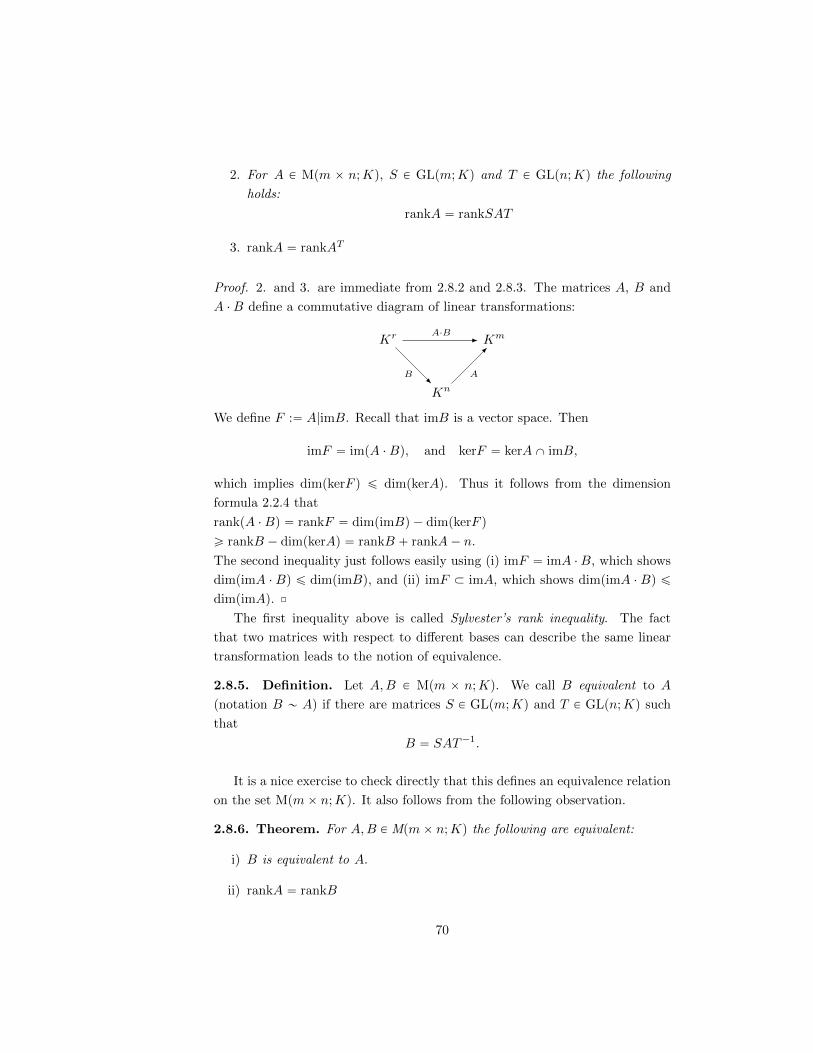
2. For A P Mpm ˆ n;Kq, S P GLpm;Kq and T P GLpn;Kq the following

holds:

rankA “ rankSAT

3. rankA “ rankAT

Proof. 2. and 3. are immediate from 2.8.2 and 2.8.3. The matrices A, B and

A ¨B define a commutative diagram of linear transformations:

Kr A¨B - Km

Kn

A

-

B -

We define F :“ A|imB. Recall that imB is a vector space. Then

imF “ impA ¨Bq, and kerF “ kerAX imB,

which implies dimpkerF q ď dimpkerAq. Thus it follows from the dimension

formula 2.2.4 that

rankpA ¨Bq “ rankF “ dimpimBq ´ dimpkerF q

ě rankB ´ dimpkerAq “ rankB ` rankA´ n.

The second inequality just follows easily using (i) imF “ imA ¨B, which shows

dimpimA ¨ Bq ď dimpimBq, and (ii) imF Ă imA, which shows dimpimA ¨ Bq ď

dimpimAq. ˝

The first inequality above is called Sylvester’s rank inequality. The fact

that two matrices with respect to different bases can describe the same linear

transformation leads to the notion of equivalence.

2.8.5. Definition. Let A,B P Mpm ˆ n;Kq. We call B equivalent to A

(notation B „ A) if there are matrices S P GLpm;Kq and T P GLpn;Kq such

that

B “ SAT´1.

It is a nice exercise to check directly that this defines an equivalence relation

on the set Mpmˆ n;Kq. It also follows from the following observation.

2.8.6. Theorem. For A,B P Mpmˆ n;Kq the following are equivalent:

i) B is equivalent to A.

ii) rankA “ rankB

70

iii) There are vector spaces V and W of dimension n and m with bases A,A1

and B,B1 and a linear transformation F : V ÑW such that

A “MAB pF q and B “MA1

B1 pF q

Thus A and B describe the same linear transformation with respect to

suitable choices of bases.

Proof. (i) ùñ (ii) follows from 2.8.3. (ii) ùñ (iii): Let pe1, . . . , enq be the

canonical basis of Kn and pe11, . . . , e1mq be the canonical basis of Km. If

r :“ rankA “ rankB

then we define

F : Kn Ñ Km

by F peiq “ e1i for i “ 1, . . . , r and F peiq “ 0 for i “ r ` 1, . . . , n. First we

consider the linear transformation

A : Kn Ñ Km

By 2.8.1 there is a commutative diagram

Kn FÝÝÝÝÑ Km

Φ

§

§

đ

§

§

đΨ

Kn AÝÝÝÝÑ Km

with isomorphisms Φ and Ψ. This means conversely that A represents F

with respect to the bases

A “ pΦ´1pe1q, . . . ,Φ´1penqq and B “ pΨ´1pe11q, . . . ,Ψ

´1pe1mqq

In the same way we get bases A1 and B1 with respect to which F is represented

by B. (iii) ùñ (i) follows from the transformation formula stated before 2.8.1

above. ˝

It follows from this theorem that the word equivalent could be replaced by

of equal rank. In Mpmˆ n;Kq there are precisely

k :“ mintm,nu ` 1

distinct equivalence classes. The special representatives˜

Ir 0

0 0

¸

, r P t0, 1, . . . , k ´ 1u

71

are called normal forms.

Given A P Mpm ˆ n;Kq we know that there exist matrices S P GLpm;Kq

and T P GLpn;Kq such that in block matrices:

SAT´1 “

˜

Ir 0

0 0

¸

where r “ rankA. The matrices S, T can be found as follows: We can first

bring A into row echelon form. The necessary row operations correspond to

multiplication from the left by elementary m-row matrices B1, . . . , Bk. These

operations can be done parallel on Im and give rise to the matrix Bk ¨ . . . ¨ B1.

Because the matrix Bk ¨ . . . ¨ B1 ¨ A has row echelon form, by using column

operations it can be brought into the form˜

Ir 0

0 0

¸

with r “ rankA. This corresponds to multiplications from the right by n-row

elementary matrices C1, . . . C`. These column operations can be done parallel

on In. Since

Bk ¨ . . . ¨B1 ¨A ¨ C1 . . . ¨ C` “

˜

Ir 0

0 0

¸

by

S :“ Bk ¨ . . . ¨B1 “ Bk ¨ . . . ¨B1 ¨ Im

and

T´1 “ C1 ¨ . . . ¨ C` “ In ¨ C1 ¨ . . . ¨ C1

we have found corresponding transformation matrices.

2.8.7. Example. Let K “ R and A “

˜

1 2 0

2 2 1

¸

. We place the identity

matrices on the corresponding side (no multiplication) and perform operations

simultaneously. A first row operation gives

1 0 1 2 0

0 1 2 2 1

1 0 1 2 0

-2 1 0 -2 1

and we get S “

˜

1 0

´2 1

¸

. Then we perform column operations:

72

1 2 0 1 0 0

0 -2 1 0 1 0

0 0 1

1 0 2 1 0 0

0 1 -2 0 0 1

0 1 0

1 0 0 1 0 -2

0 1 -2 0 0 1

0 1 0

1 0 0 1 0 -2

0 1 0 1 0 1

0 1 2

from which we read off

SAT´1 “

˜

1 0 0

0 1 0

¸

, T´1 “

¨

˚

˝

1 0 ´2

1 0 1

0 1 2

˛

‹

‚

If

D “

˜

Ir 0

0 0

¸

we also get bases A respectively B of Kn respectively Km such that A is repre-

sented by D with respect to these bases. For this consider the diagram

Kn DÝÝÝÝÑ Km

T

İ

§

§

İ

§

§S

Kn AÝÝÝÝÑ Km

which is commutative because of D “ SAT´1. Thus A respectively B are the

images of the canonical bases K respectively K1 of Kn respectively Km under

the isomorphisms T´1 and S´1. Also A and B can be found as column vectors

of T´1 and S´1. We need to invert S for this. In our example

S´1 “

˜

1 0

2 1

¸

and thus

pp1, 0, 0q, p0, 0, 1q, p´2, 1, 2qq and pp1, 2q, p0, 1qq

73

are the bases we want. It can be checked:

A ¨

¨

˚

˝

1

0

0

˛

‹

‚

“

˜

1

2

¸

, A ¨

¨

˚

˝

0

0

1

˛

‹

‚

“

˜

0

1

¸

and A ¨

¨

˚

˝

´2

1

2

˛

‹

‚

“

˜

0

0

¸

Of course the procedure can be modified to give directly S´1 and the additional

inversion is not necessary.

Usually endomorphisms are represented with respect to a single basis. The

question how to find a convenient basis in this situation is much more difficult

and will be discussed in Chapter 5.

74

Chapter 3

Dual vector spaces and

Linear systems of equations

3.1 Dual vector spaces

3.1.1. Definition. For V a K-vector space, the vector space

V ˚ :“ LKpV,Kq

of all linear transformations ϕ : V Ñ K is called the dual vector space (or briefly

the dual space of V ). Each ϕ P V ˚ is called a linear functional on V .

3.1.2. Examples. (i) Let V “ Kn and a1, . . . , an P K then

ϕ : Kn Ñ K, px1, . . . , xnq ÞÑ a1x1 ` . . .` anxn

defines a linear functional ϕ P pKnq˚. The relation with linear systems of

equations is easy to see. The solution set of

a11x1 ` . . .` a1nxn “ 0...

......

am1x1 ` . . .` amnxn “ 0

is the set of vectors px1, . . . , xnq P Kn mapping to 0 under the m linear func-

tionalspx1, . . . , xnq ÞÑ a11x1 ` . . .` a1nxn

......

...

px1, . . . , xnq ÞÑ am1x1 ` . . .` amnxn

75

A particular property of the system of equations above is that the conditions

can be changed in certain ways without changing the solution set. Here is an

example in a very special case, namely for n “ 2, m “ 1 and K “ R. Then,

for given a, b P R we want to find all px, yq P R2 with ax ` by “ 0, so we are

interested in the space of solutions

W :“ tpx, yq P R2 : ax` by “ 0u.

The pair pa, bq can be considered to be element of a vector space, but in a

different way than px, yq. The pair px, yq is an element of the original R2 while

pa, bq acts as a linear functional

ϕ : R2 Ñ R, px, yq ÞÑ ax` by,

and thus is an element of pR2q˚. This would all just be formal nonsense if we

could not connect the vector space structure of pR2q˚ with the equation (or

more generally with the system of equations). In our case this is particularly

simple. Consider the space W o :“ spanpϕq Ă pR2q˚, i. e. the set of all linear

functionals:

λϕ : R2 Ñ R, px, yq ÞÑ λax` λby,

with λ P R arbitrarily. If pa, bq “ p0, 0q then W o is the zero space. If pa, bq ‰

p0, 0q then W o and W are 1-dimensional subspaces. In particular, W Ă R2 is a

line. If we choose a particular λϕ PW o, different from zero (which corresponds

to λ ‰ 0) then the equation corresponding to the linear functional is:

λax` λby “ 0,

and has of course also solution set W . It is this relation between subspaces

W Ă R2 andW o Ă pR2q˚ which reveals the connection between a linear equation

and its set of solutions. A similar relation will be found for systems of linear

equations as above.

(ii) Let CpIq be the vector space of all continuous functions on the interval

I “ r0, 1s. Let

CpIq Ñ R, f ÞÑż 1

0

fpxqdx

be a linear functional on CpIq. If a P r0, 1s then also

δa : CpIq Ñ R, f ÞÑ fpaq

is a linear functional, called the Dirac δ-functional.

76

(iii) Let DpRq be the vector space of all differentiable functions and a P R. Then

DpRq Ñ R, f ÞÑ f 1paq

is a linear functional.

3.1.2. Theorem. Let V be a finite dimensional K-vector space and pv1, . . . , vnq

be a basis of V . Then there are uniquely determined linear functionals v˚1 , . . . , v˚n P

V ˚ defined by

v˚i pvjq “ δij

where δij “ 1 if i “ j and δij “ 0 if i ‰ j is the Kronecker-symbol. Further-

more, pv˚1 , . . . , v˚nq is a basis of V ˚ and thus

dimV ˚ “ dimV.

The basis B˚ :“ pv˚1 , . . . , v˚nq is called the basis dual to the basis B “ pv1, . . . , vnq

of V .

Proof. Existence and uniqueness of v˚1 , . . . , v˚n follows from 2.1.4. It remains to

show that those form a basis. For ϕ P V ˚ define

λi :“ ϕpviq for i “ 1, . . . , n and ψ :“ λ1v˚1 ` . . .` λnv

˚n

Then for j “ 1, . . . , n

ψpvjq “nÿ

i“1

λiv˚i pvjq “

nÿ

i“1

λiδij “ λj “ ϕpvjq.

Because ψ and ϕ have the same images on a basis by 2.1.4 it follows ψ “ ϕ.

Thus V ˚ is spanned by v˚1 , . . . , v˚n. This proves (B1). Suppose that

nÿ

i“1

λiv˚i “ 0.

If we apply both sides to vj the left hand side becomes λj and the right hand

side is 0. Thus λj “ 0 for j “ 1, . . . , n and (B2) follows. ˝

3.1.3. Corollary. Let V be a finite dimensional K-vector space. Then for each

0 ‰ v P V there exists ϕ P V ˚ such that ϕpvq ‰ 0.

Proof. Complete pvq to a basis pv1 “ v, v2, . . . , vnq of V and consider the dual

basis. Then v˚1 pvq “ 1. ˝

3.1.4. Remark. While 3.1.2. does not hold for infinite dimensional vector

spaces the statement of 3.1.3 remains true. In fact, by basis completion we can

77

still construct a basis pv, viqiPI including 0 ‰ v and then define by 2.1.4 the

linear transformation F : V Ñ K by F pvq “ 1 and F pviq “ 0 for all i P I.

Note that the linear transformation constructed from a single vector 0 ‰ v in

this way is not canonically defined because it will depend on the choice of basis

completion.

Suppose V is a finite dimensional K-vector space and A “ pv1, . . . , vnq is

a basis. Using the dual basis pv˚1 , . . . , v˚nq we get by 2.1.4 a uniquely defined

isomorphism

ΨA : V Ñ V ˚, vi ÞÑ v˚i .

This isomorphism is not canonical in the sense that it does depend on the choice

of basis. If B “ pw1, . . . , wnq is another basis and

ΨB : V Ñ V ˚

is the corresponding isomorphism then in general ΨA ‰ ΨB. Consider for

example w1 “ λ1v1 ` . . .` λnvn then

ΨApw1q “ λ1v˚1 ` . . .` λnv

˚n

and application of this linear transformation to w1 gives

ΨApw1qpw1q “ λ21 ` . . .` λ

2n.

On the other hand

ΨBpw1qpw1q “ w˚1 pw1q “ 1.

For V “ Kn on the other hand we can use the canonical basis pe1, . . . , enq. The

corresponding dual basis pe˚1 , . . . , e˚nq then is called the canonical basis of pKnq˚

and

Ψ : Kn Ñ pKnq˚, ei ÞÑ e˚i

is called the canonical isomorphism. The usual convention in this case is to

consider vectors in Kn as column vectors and the linear functionals in pKnq˚

as row vectors. Thus if

x “ x1e1 ` . . .` xnen P Kn and

ϕ “ a1e˚1 ` . . .` ane

˚n,

then we write

x “

¨

˚

˚

˝

x1

...

xn

˛

‹

‹

‚

“ px1, . . . , xnqT and ϕ “ pa1, . . . , anq.

78

Then

ϕpxq “ a1x1 ` . . .` anxn “ pa1, . . . , anq

¨

˚

˚

˝

x1

...

xn

˛

‹

‹

‚

,

and thus application of the functional corresponds to matrix multiplication of a

row vector and a column vector. Thus we will in the following identify Mpn ˆ

1;Kq with Kn and Mp1ˆ n;Kq with pKnq˚. The canonical isomorphism

Ψ : Mpnˆ 1;Kq “ Kn Ñ pKnq˚ “ Mp1ˆ n;Kq

then corresponds to transposition of matrices. Of course transposing twice is

not doing anything.

If V ˚ is the dual space of a K-vector space V then we can define pV ˚q˚,

the dual space of V ˚, called the bidual of V and is usually written V ˚˚. The

elements of the bidual assign to each linear transformation ϕ : V Ñ K a scalar.

For fixed v P V in this way we can assign to ϕ P V ˚ the scalar ϕpvq.

3.1.5. Theorem. Let V be a K-vector space. Then the map

ι : V Ñ V ˚˚, v ÞÑ ιv,

with ιvpϕq :“ ϕpvq defines a monomorphism of K-vector spaces. If dimV ă 8

then ι is an isomorphism.

Proof. First we show that for each v P V the map

ιv : V ˚ Ñ K, ϕ ÞÑ ϕpvq

is linear, and thus ιv P V˚˚. Given ϕ,ψ P V ˚ and λ, µ P K we have ιvpλϕ `

µψq “ pλϕ ` µψqpvq “ λϕpvq ` µψpvq “ λιvpϕq ` µιvpψq. Now we show that

ι is a linear transformation. Let v, w P V and λ, µ P K. Then ιλv`µwpϕq “

ϕpλv ` µwq “ λϕpvq ` µϕpwq “ λιvpϕq ` µιwpϕq “ pλιv ` µιwqpϕq. Thus

ιλv`µw “ λιv ` µιw, and ι is linear. To see that ι is injective choose v P V such

that ιv “ 0, i. e. ιvpϕq “ 0 for all ϕ P V ˚. By 3.1.3 and the following Remark

we know that v “ 0. If V is finite dimensional then by 3.1.2 it follows that

dimV “ dimV ˚ “ dimV ˚˚

and by 2.6.2 it follows that ι is an isomorphism. ˝

It is important to recognize that the linear transformation ι : V Ñ V ˚˚ is

canonical in the sense that it does not depend on a choice of basis. If V is finite

79

dimensional we can in this way identify V and V ˚˚, i. e. each element of V can

also be considered an element of V ˚˚ and vice versa. This can be indicated

using the suggestive notation

vpϕq “ ϕpvq.

Let V be a K-vector space and W Ă V a subspace. Then

W o :“ tϕ P V ˚ : ϕpwq “ 0 for all w PW u Ă V ˚

is called the space dual to W . It is easy to see that W o is a subspace: Of course

the zero transformation is in W o. If ϕ,ψ PW o and w PW then

pϕ` ψqpwq “ ϕpwq ` ψpwq “ 0

and so ϕ ` ψ P W o and similarly λϕ P W o. Now recall from the above our

notation for writing elements in Kn and pKnq˚. If 0 ‰ px, yqT P R2 and

W :“ R ¨ px, yqT

is the line spanned by px, yqT then

W o “ tpa, bq P pR2q˚ : pa, bq ¨

˜

x

y

¸

“ 0u Ă pR2q˚.

If we use the natural identification of column and row vectors and thus identify

R2 and pR2q˚ we see that W o is the line perpendicular to W .

o

˜

x

y

¸

o

6

-

W R2

pa, bq o

o

6

-

pR2q˚ W o

80

In a different way, each element of W o represents a linear equation satisfied

by all vectors in W . We will see how to get back from W o to W as the set of

solutions of the equations represented by W o.

3.1.6. Theorem. Let W be subspace of the finite dimensional K-vector space

V , pw1, . . . , wkq a basis of W and pw1, . . . , wk, v1, . . . , vrq a basis of V . Then

pv˚1 , . . . , v˚r q is a basis of W o. In particular:

dimW ` dimW o “ dimV.

Proof. pv˚1 , . . . , v˚r q is a subfamily of the dual basis pw˚1 , . . . w

˚k , v

˚1 , . . . , v

˚r q and

thus linearly independent. It suffices to show

W o “ spanpv˚1 , . . . , v˚r q.

Since v˚i pwjq “ 0 for 1 ď i ď r and 1 ď j ď k we have spanpv˚1 , . . . , v˚r q Ă W o.

Conversely, let ϕ PW o. Then there exist µ1, . . . , µk, λ1, . . . , λr P K such that

ϕ “ µ1w˚1 ` . . .` µkw

˚k ` λ1v

˚1 ` . . .` λrv

˚r .

For 1 ď i ď k, by substituting wi:

0 “ ϕpwiq “ µi,

and thus ϕ P spanpv˚1 , . . . , v˚r q. ˝

3.1.7. Corollary. Let V be a finite dimensional K-vector space and let V ˚˚

be identified with V according to 3.1.5. Then for each subspace W Ă V :

pW oqo “W

.

Proof. Let w P W and ϕ P W o then wpϕq “ ϕpwq “ 0 and thus w P pW oqo.

Thus W Ă pW oqo. Since dimV “ dimV ˚ it follows from 3.1.6 that dimW “

dimpW oqo and thus the claim. ˝

The above discussion is an abstract interpretation of linear systems of equa-

tions. Corresponding to the system of equations we have a subspace U of V ˚

and the solution set is the vector space Uo Ă V . Conversely to each subspace

W Ă V there corresponds the set W o Ă V ˚ of linear equations with solution

set W .

81

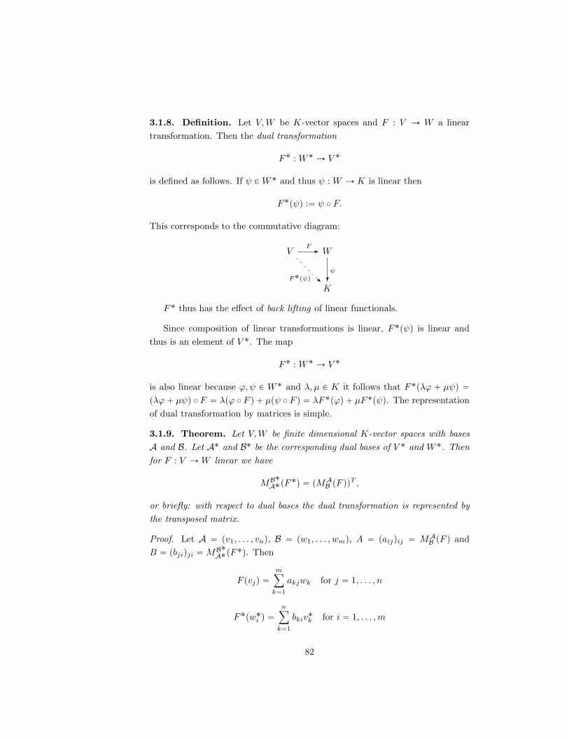
3.1.8. Definition. Let V,W be K-vector spaces and F : V Ñ W a linear

transformation. Then the dual transformation

F˚ : W˚ Ñ V ˚

is defined as follows. If ψ PW˚ and thus ψ : W Ñ K is linear then

F˚pψq :“ ψ ˝ F.

This corresponds to the commutative diagram:

VF- W

K

ψ

?F˚pψq-

F˚ thus has the effect of back lifting of linear functionals.

Since composition of linear transformations is linear, F˚pψq is linear and

thus is an element of V ˚. The map

F˚ : W˚ Ñ V ˚

is also linear because ϕ,ψ P W˚ and λ, µ P K it follows that F˚pλϕ ` µψq “

pλϕ` µψq ˝ F “ λpϕ ˝ F q ` µpψ ˝ F q “ λF˚pϕq ` µF˚pψq. The representation

of dual transformation by matrices is simple.

3.1.9. Theorem. Let V,W be finite dimensional K-vector spaces with bases

A and B. Let A˚ and B˚ be the corresponding dual bases of V ˚ and W˚. Then

for F : V ÑW linear we have

MB˚A˚pF

˚q “ pMAB pF qq

T ,

or briefly: with respect to dual bases the dual transformation is represented by

the transposed matrix.

Proof. Let A “ pv1, . . . , vnq, B “ pw1, . . . , wmq, A “ paijqij “ MAB pF q and

B “ pbjiqji “MB˚A˚pF

˚q. Then

F pvjq “mÿ

k“1

akjwk for j “ 1, . . . , n

F˚pw˚i q “nÿ

k“1

bkiv˚k for i “ 1, . . . ,m

82

By the definition of dual bases:

w˚i pF pvjqq “ aij and F˚pw˚i qpvjq “ bji.

By definition of F˚ we have F˚pw˚i q “ w˚i ˝ F and thus aij “ bji. ˝

3.1.10. Corollary. Let V,W be finite dimensional K-vector spaces. Then the

map

LKpV,W q Ñ LKpW˚, V ˚q, F ÞÑ F˚

is an isomorphism.

Proof. Let n :“ dimV and m :“ dimW . Then by 3.1.9 there is the commutative

diagramLKpV,W q ÝÝÝÝÑ LKpW

˚, V ˚q

MAB

§

§

đ

§

§

đMB˚

A˚

Mpmˆ n;Kq ÝÝÝÝÑ Mpnˆ n;Kq

with the top transformation mapping F to F˚ and the bottom transforma-

tion mapping A to AT . By 2.1.7 (iii) transposition is an isomorphism and by

2.4.1 the maps MAB and MB˚

A˚ are isomorphisms. Thus the given map is an

isomorphism. ˝

3.1.11. Lemma. Let F : V Ñ W be a linear transformation between finite

dimensional vector spaces. Then

imF˚ “ pkerFqo

Proof. Ă: If ϕ P imF˚ then there exists ψ P W˚ such that ϕ “ F˚pψq, which

means ϕ “ ψ ˝ F . If v P kerF then ϕpvq “ ψpF pvqq “ ψp0q “ 0. Thus

ϕ P pkerFqo. Ą: Conversely let ϕ P pkerF qo. We need ψ P W˚ such that

ϕ “ F˚pψq, which means that the diagram

VF - W

K

ψ�

ϕ -

commutes. For the construction of ψ we choose following 2.2.4 and 1.5.16

bases pu1, . . . , uk, v1, . . . , vrq of V and pw1, . . . , wr, wr`1, . . . , wmq of W such that

pu1, . . . , ukq is a basis of kerF , pw1, . . . , wrq is a basis of imF and wi “ F pviq

83

for i “ 1, . . . , r. Then by 2.1.4

ψpwiq “

$

&

%

ϕpwiq if i “ 1, . . . r

0 if i “ r ` 1, . . . ,m

defines a linear functional ψ P W˚. For i “ 1, . . . r because of ui P kerF and

ϕ P pkerF qo, we have

F˚pψqpuiq “ ψpF puiqq “ ψp0q “ 0 “ ϕpuiq

and for j “ 1, . . . , r by the definition of ψ

F˚pψqpvjq “ ψpF pvjqq “ ψpwjq “ ϕpvjq.

Since F˚pψq and ϕ coincide on a basis they are the same linear transformation.

˝

3.1.12. Corollary. For each matrix A P Mpmˆ n;Kq we have

col-rankA “ row-rankA

Proof. Using 3.1.10 we identify A respectively AT with the corresponding linear

transformations

A : Kn Ñ Km and AT : pKmq˚ Ñ pKnq˚

Then

col-rankA “ dimA

“ n´ dimpkerAq by 2.2.4

“ dimppkerAqoq by 3.1.6

“ dimpimAT q by 3.1.11

“ col-rankpAT q

“ row-rankpAq

3.1.13. Example. Consider in R3 the two linear functionals:

ϕ : R3 Ñ R, x “ px1, x2, x3q ÞÑ a1x1 ` a2x2 ` a3x3, and

ψ : R3 Ñ R, x “ px1, x2, x3q ÞÑ b1x1 ` b2x2 ` b3x3

and we consider the set

W :“ tx P R3 : ϕpxq “ ψpxq “ 0u,

84

which is the simultaneous set of zeroes of the linear equations defines by ϕ and

ψ. We want to show that in general W is a line. W is the kernel of the linear

transformation

F : R3 Ñ R2, x ÞÑ pϕpxq, ψpxqq.

It follows easily from the definitions that

imF˚ “ spanpϕ,ψq Ă pR3q˚.

(Calculate F˚ on the canonical dual basis e˚1 and e˚2 of pR2q˚.) By 3.1.6 and

3.1.11

p˚q dimW “ 3´ dimpimF˚q.

Thus W is a line if and only if ϕ and ψ are linearly independent, which means

that the two vectors

pa1, a2, a3q and pb1, b2, b3q

are linearly independent. This can be seen as the general case. If ϕ and ψ

are linearly dependent but not both 0 then W is according to (*) a plane. If

ϕ “ ψ “ 0 then W “ R3.

3.2 Homogeneous linear systems of equations

In the solution of linear systems of equations we first consider the special case of

homogeneous systems. We will see that the general case can be reduced to this

case. Let R be a commutative unital ring and for i “ 1, . . .m and j “ 1, . . . , n

be given elements aij P R. We call the system of equations (*):

a11x1 ` . . .` a1nxn “ 0

......

...

am1x1 ` . . .` amnxn “ 0

a homogeneous linear system of equations in the unknowns x1, . . . , xn with co-

efficients in R. The matrix¨

˚

˚

˝

a11 . . . a1n

......

am1 . . . amn

˛

‹

‹

‚

is called its coefficient matrix. If we put x “ px1, . . . , xnqT then (*) can be

written in a compact form as

A ¨ x “ 0.

85

A column vector x P Rn then is called solution of (*) if

A ¨ x “ 0.

The solution set of (*) is the set

W “ tx P Rn : A ¨ x “ 0u.

The notion of unknowns can be formalized but we will not be discussing this.

In the case that R is a field K the solution set is a subspace of the vector space

Kn and is called the solution space.

3.2.1. Theorem. If A P Mpmˆ n;Kq then the solution space

W “ tx P Kn : A ¨ x “ 0u

is a subspace of dimension

dimW “ n´ rankA

Proof. W is the kernel of the linear transformation

A : Kn Ñ Km, x ÞÑ A ¨ x

and thus the claim follows from 2.2.4. ˝

Solving a system of equations means to give a procedure to find all solutions

in an explicit form. In the case of a homogeneous linear system of equations it

suffices to give a basis pw1, . . . , wkq of the solution space W Ă Kn. Then

W “ Kw1 ‘ . . .‘Kwk.

3.2.2. Lemma. Let A P Mpm ˆ n;Kq and S P GLpm;Kq. Then the linear

systems of equation A ¨ x “ 0 and pSAq ¨ x “ 0 have the same solution spaces.

Proof. If A ¨x “ 0 then also pSAq¨x “ S ¨pA ¨xq “ 0. Conversely, if pS ¨Aq¨x “ 0

then also A ¨ x “ pS´1SAq ¨ x “ 0. ˝

As we have seen in 2.7 elementary row operations correspond to multiplica-

tion by invertible matrices from the left. Thus we have:

3.2.3. Corollary. Let A P Mpm ˆ n;Kq and B P Mpm ˆ n;Kq be resulting

by elementary row operations from A. Then the linear systems of equations

A ¨ x “ 0 and B ¨ x “ 0 have the same solution sets. ˝

86

Important: Column operations on the coefficient matrix change the solution

space in general. Only permutations of columns are not problematic because

they correspond to renaming of the unknowns.

We now have available all technical tools to determine solution spaces W .

First we bring A into row echelon form by elementary row operations, see 2.5.3.

Here, see 3.1.12,

r “ col-rankA “ row-rankA

and

r “ rankA and dimW “ n´ r “: k.

The corresponding system of equations B ¨ x “ 0 is called the reduced system.

The equality of row-rank and column-rank is essential. From the matrix B we

read off the row-rank, for the dimension of W the column-rank is responsible. It

suffices to determine explicitly a basis of W . For simplicity we can assume j1 “

1, . . . , jr “ r, which corresponds to renumbering the unknowns, i. e. permutation

of columns. Let

B “

¨

˚

˚

˚

˝

b11 . . . . . .

¨

0 ¨

brr . . .

˛

‹

‹

‹

‚

The unknowns xr`1, . . . , xn are essentially different from the x1, . . . , xr. While

xr`1, . . . , xn are free parameters, the x1, . . . , xr are determined by those. More

precisely: For each choice of λ1, . . . , λk P K there is a unique vector

px1, . . . , xr, λ1, . . . , λkq PW.

The calculation of x1, . . . , xr for the given λ1, . . . , λk can be done recursively.

The r-th row of B is

brrxr ` br,r`1xr`1 ` . . .` brnxn “ 0

and from this we can calculate xr because brr ‰ 0. In the same way we can

calculate xr´1 using the pr ´ 1q-st row, and finally from the first row x1 (often

renumbering of the unknowns is not done explicitly). In summary we get a

linear transformation

G : Kk Ñ Kn, pλ1, . . . , λkq ÞÑ px1, . . . , xr, λ1, . . . , λkq.

This linear transformation is obviously injective and has image W because

dimW “ k. Thus if pe1, . . . , ekq is the canonical basis of Kk then

pGpe1q, . . . , Gpekqq

87

is a basis of W . For explicit examples check on some free on-line books:


or see this page:

http://www.sosmath.com/matrix/system1/system1.html

You will also find further practical hints about finding solutions on these or

other pages.

Now we want to study how to find for a given subspace W a system of

equations with solution set W .

3.2.4. Theorem. Let W Ă V be subspace of a finite dimensional vector space

V and let ϕ1, . . . , ϕr P V˚. Then the following are equivalent:

(i) W “ tv P V : ϕ1pvq “ . . . “ ϕrpvq “ 0u, i. e. W is solution space of the

linear system of equations ϕ1pvq “ . . . “ ϕrpvq “ 0.

(ii) W o “ spanpϕ1, . . . , ϕrq, i. e. the linear functionals ϕ1, . . . , ϕr span the

subspace of V ˚ orthogonal to W .

In particular r :“ dimV ´ dimW is the smallest number of necessary linear

equations.

Proof. Let U :“ spanpϕ1, . . . , ϕrq Ă V ˚. As in 3.1.5 we identify V and V ˚˚.

Then condition (i) is equivalent to W “ Uo while condition (ii) is equivalent to

W 0 “ U . But by 3.1.7 these are equivalent. By 3.1.6

dimW o “ dimV ´ dimW

and thus r :“ dimV ´ dimW is minimal. ˝

Let W be a subspace of Kn then we want to determine a basis of W o Ă

pKnq˚. If pw1, . . . , wkq is a basis of W then

W o “ tϕ P pKnq˚ : ϕpwq “ 0 for all w PW u

“ tϕ P pKnq˚ : ϕpw1q “ . . . “ ϕpwkq “ 0u

Using the conventions from 3.1:

w1 “

¨

˚

˚

˝

b11

...

b1n

˛

‹

‹

‚

, . . . , wk “

¨

˚

˚

˝

bk1

...

bkn

˛

‹

‹

‚

88


http://www.sosmath.com/matrix/system1/system1.html

and

B “

¨

˚

˚

˝

b11 . . . bk1

......

b1n . . . bkn

˛

‹

‹

‚

the matrix with the columns determined by coefficients of the basis vectors of

W . Let

a “ pa1, . . . , anq

be the linear functional ϕ written as row vector. The conditions for W o then

can be written as a ¨B “ 0, or equivalently

BTaT “ 0.

Thus W o is solution space of this homogeneous linear system of equations. Since

rankBT “ k

it has dimension r :“ n´ k, and as explained above one can find a basis

ϕ1 “ pa11, . . . , a1nq,

......

ϕr “ par1, . . . , arnq

of W o. If

A “

¨

˚

˚

˝

a11 . . . a1n

......

ar1 . . . arn

˛

‹

‹

‚

then W is by 3.2.4 the solution space of the homogeneous linear system of

equations

A ¨ x “ 0.

Furthermore, the matrix A has rank r “ n´ k and A ¨B “ 0, and thus

0 “ rankA` rankB ´ n “ rankA ¨B

From this it follows that Sylvester’s rank inequality in 2.8.4 is sharp (for all and

given B).

89

3.3 Affine subspaces and inhomogeneous linear

systems of equations

A linear system of equations (**):

a11x1 ` . . . a1nxn “ b1...

......

am1 ` . . . amnxn “ bm

with coefficients aij and bi from a field K is inhomogeneous if

pb1, . . . , bmq ‰ p0, . . . , 0q.

Again we denote by A “ paijqij the coefficient matrix and with

b “ pb1, . . . , bmqT P Km

the column vector of coefficients of the right hand side of the equation. Then

the system (**) can be written

A ¨ x “ b.

The solution set

X “ tx P Kn : A ¨ x “ bu

is for b ‰ 0 no longer a subspace because 0 R X. In the special case K “ R,

n “ 2 and m “ 1

X “ tx “ px1, x2qT : a1x1 ` a2x2 “ bu

for pa1, a2q ‰ p0, 0q and b ‰ 0 is a line, which is not through the origin. This

line we can imagine is defined from

W “ tx “ px1, x2qT : a1x1 ` a2x2 “ 0u

by a parallel translation. For a linear system of equations (**):

A ¨ x “ b

we call (*):

A ¨ x “ 0

90

the associated homogeneous system of equations. We will show now that also

in the general case the solution set of (**) can be determined from (*) by a

translation.

3.3.1. Definition. A subset X of a vector space V is called an affine subspace

if there exists v P V and a subspace W Ă V such that

X “ v `W “ tu P V : there exists w PW such that u “ v ` wu

It will be convenient also to consider the empty set as an affine subspace.

Examples of affine subspaces of Rn are points, planes, lines.

3.3.2. Remarks. Let X “ v ` W Ă V be an affine subspace. Then the

following holds:

a) For each v1 P X

X “ v1 `W

b) If v1 P V and W 1 Ă V is a subspace with

v `W “ v1 `W 1

then W “W 1 and v1 ´ v PW .

Proof. a): We write v1 “ v ` w1. Then

X Ă v1 `W, because u P X ùñ u “ v ` w with w PW ùñ u P v1 `W

v1 `W Ă X, because u “ v1 ` w P v1 `W ùñ u “ v ` pw ` w1q P v `W.

b): Define

X ´X “ tu´ u1 : u, u1 P Xu

to be the set of all differences of vectors in X (please do not confuse with the

set difference XzX “ H.) Then

X ´X “W and X ´X “W 1

and thus W “W 1. Since v `W “ v1 `W there is w PW such that v1 ´ v “ w

and thus v1 “ v ` w PW . ˝

Since for an affine subspace X “ v `W the subspace W is uniquely deter-

mined we can define

dimX :“ dimW.

91

3.3.3. Lemma. Let F : V Ñ W be a linear transformation. Then for each

w P W the set F´1pwq is an affine subspace. If F´1pwq ‰ H and v P F´1pwq

then

p:q F´1pwq “ v ` kerF.

Proof. If X “ F´1pwq “ H the claim follows by the above convention. Other-

wise let v P X and we have to show (:) above. If u, v P X then u “ v` pu´ vq.

Since

F pu´ vq “ F puq ´ F pvq “ w ´ w “ 0

we have u´ v P kerF and u P v ` kerF . If u “ v ` v1 P v ` kerF then

F puq “ F pvq ` F pv1q “ w ` 0 “ w,

and thus u P X. ˝

3.3.4. Corollary. If A P Mpmˆn;Kq and b P Km then we consider the linear

system of equations (**):A ¨ x “ b and the associated homogeneous system of

equations (*): A ¨ x “ 0. Let X “ tx P Kn : A ¨ x “ bu the solution space of

(**) and W “ tx P Kn : A ¨ x “ 0u be the solution space of (*). If X ‰ H then

X “ v `W

Briefly: The general solution of an inhomogeneous system of equations is given

by adding a special solution to the general solution of the associated homogeneous

system of equations. In particular X Ă Kn is an affine subspace of dimension

dimX “ n´ rankA

Proof. Consider the linear transformation defined by A:

F : Kn Ñ Km, x ÞÑ A ¨ x.

Then

W “ kerF “ F´1p0q and X “ F´1pbq

and the claim follows from 3.3.3. ˝

3.3.5. Remark. It is possible that W ‰ H but X “ H. The simplest example

is form “ n “ 1 and the equation 0¨x “ 1. We haveW “ tx P K : 0¨x “ 0u “ K

but X “ tx P K : 0 ¨ x “ 1u “ H. Note that the homogeneous system of

equations always has the trivial solution 0.

92

In order to give a simple criterion for the existence of at least one solution

we consider the extended coefficient matrix

A1 :“ pA, bq “

¨

˚

˚

˝

a11 . . . a1n b1...

......

am1 . . . amn bm

˛

‹

‹

‚

P Mpmˆ pn` 1q;Kq.

3.3.6. Theorem. The solution space of the linear system of equations

A ¨ x “ b

is not empty if and only if

rankA “ rankpA, bq

(This condition has been found in 1875/76 by G. Fontene, E. Rouche and F. G.

Frobenius.)

Proof. A describes the linear transformation

A : Kn Ñ Km, x ÞÑ A ¨ x

and pA, bq describes the linear transformation

A1 : Kn`1 Ñ Km, x1 ÞÑ A1 ¨ x1.

If pe1, . . . , enq and pe11, . . . , e1n, e

1n`1q are the canonical bases then

Ape1q “ A1pe11q, . . . , Apenq “ A1pe1nq and A1pe1n`1q “ b

Thus b is in the image of A1 by construction while this has to be decided for A.

Since imA Ă imA1 we have

rankA ď rankA1.

Thus rankA “ rankA1 is equivalent to

rankA ě rankA1, i. e. imA Ą imA1

which by the definition of A1 is equivalent to b P imA, and this proves the claim.

˝

A nice case is if the solution space of a linear system of equations A ¨ x “ b

for fixed A P Mpm ˆ n;Kq is non-empty for all b P Km. In this case we say

93

that the system of equations is universally solvable. This means that the linear

transformation

A : Kn Ñ Km

is onto. From this the following is immediate.

3.3.7. Remarks. (a) If A P Mpmˆ n;Kq then the following are equivalent:

(i) The linear system of equations A ¨ x “ b is universally solvable.

(ii) rankA “ m

If the solution space of a linear system of equations consists of just one element

we say that the system is uniquely solvable. From the previous we have

(b) For A P Mpmˆ n;Kq and b P Km the following are equivalent:

(i) The linear system A ¨ x “ b is uniquely solvable.

(ii) rankA “ rankpA, bq “ n.

In this case the corresponding homogeneous system A ¨x “ 0 has only the trivial

solution.

3.4 Practical methods for solving linear systems

The method described in 3.2 for solving homogeneous systems can easily be

modified to the inhomogeneous case. Given is A ¨ x “ b with A P Mpmˆ n;Kq

and b P Km. We begin with the extended coefficient matrix A1 “ pA, bq and

bring it into row echelon form:

¨

˚

˚

˚

˚

˚

˚

˚

˚

˚

˚

˚

˚

˝

. . . 0 b1j1 ˚ ˚ ˚ ˚ . . . ˚ c1

. . . . . . 0 . . . 0 b2j2 ˚ . . . ˚ c2...

...... 0

...

0 0 0 0 0 . . . 0 brjr ˚ cr

0 0 0 0 0 . . . 0 0 0 cr`1

......

......

......

......

...

0 0 0 . . . 0 0 0 0 0 cm

˛

‹

‹

‹

‹

‹

‹

‹

‹

‹

‹

‹

‹

‚

“: pB, cq

with b1j1 ‰ 0, . . . , brjr ‰ 0. Then rankA “ r and because of rankpA, bq “

rankpB, cq we have

rankpA, bq “ rankAðñ cr`1 “ . . . “ cm “ 0

94

Thus the coefficients cr`1, . . . , cm determine whether the system has a solution.

In the case

rankpA, bq ą rankA

no solution can exist, which can now be seen directly. If rankpA, bq ą r then we

can assume, after renumbering, cr`1 ‰ 0. In the pr ` 1q-st row we then have

the equation

0x1 ` . . .` 0xn “ cr`1,

which has no solutions. If r “ m then the coefficients cr`1, . . . , cm do not

appear. In this case, as pointed out in 3.3.7 the system is universally solvable.

In order to describe X we first find a special solution v P X. As noted in 3.2

the unknowns xj with

j R tj1, . . . , jru

are free parameters. For the simplification of notation we again assume j1 “

1, . . . , jr “ r. To find a special solution we set

xr`1 “ . . . “ xn “ 0.

Then we read from the r-th row of pB, cq

brrxr “ cr

and from this we calculate xr. Similarly we get xr´1, . . . , x1, and thus a special

solution

v “ px1, . . . , xr, 0, . . . , 0q

of the system of equations B ¨ x “ c. Since pB, cq is the result of row operations

on pA, bq by 2.7.2 there is a matrix S P GLpm;Kq such that

pB, cq “ S ¨ pA, bq “ pSA, Sbq.

Thus

Av “ S´1SAv “ S´1Bv “ S´1c “ S´1Sb “ b

and v is also a special solution of A ¨ x “ b. Now we can determine the general

solution of A ¨ x “ 0 as in 3.2 and thus get by 3.3.4 the general solution.

3.4.1. Example. Consider the linear system of equations with coefficients in

R:

x1 ´ 2x2 ` x3 “ 1

x1 ´ 2x2 ´ x4 “ 2

x3 ` x4 “ ´1

95

we get the extended matrix

pA, bq “

¨

˚

˝

1 ´2 1 0 1

1 ´2 0 ´1 2

0 0 1 1 ´1

˛

‹

‚

,

which by elementary row operations becomes

pB, cq “

¨

˚

˝

1 ´2 1 0 1

0 0 1 1 ´1

0 0 0 0 0

˛

‹

‚

Since r “ rankA “ rankpA, bq “ 2 the system has a solution, and for the solution

space X we have

dimX “ n´ r “ 4´ 2 “ 2

Furthermore j1 “ 1 and j2 “ 3. For the calculation of a special solution we set

x2 “ x4 “ 0. Then we get

x3 “ ´1, x1 ` x3 “ 1, thus x1 “ 1´ x3 “ 1` 1 “ 2,

and we get

v “ p2, 0,´1, 0q.

For the general solution of the associated homogeneous system we set x2 “ λ1

and x4 “ λ2; then we get

x3 “ ´λ2, x1 ´ 2λ1 ` x3 “ 0, thus x1 “ 2λ1 ` λ2

and

x “ p2λ1 ` λ2, λ1,´λ2, λ2q

for the general solution of the homogeneous system. The parameter represen-

tation of the general solution of the given system thus is

p2` 2λ1 ` λ2, λ1,´1´ λ2, λ2q

or

X “ p2, 0,´1, 0q ` Rp2, 1, 0, 0q ` Rp1, 0,´1, 1q

For many further examples how to use the above results we refer to the

previously mentioned web resources.

We conclude with a description of affine spaces by systems of equations.

96

3.4.2. Theorem. Let V be an n-dimensional K-vector space, X Ă V a

k-dimensional affine subspace and r :“ n´ k. Then there are linear functionals

ϕ1, . . . , ϕr P V˚ and b1, . . . , br P K with

X “ tu P V : ϕ1puq “ b1, . . . , ϕrpuq “ bru

and r is minimal with respect to this property.

Proof. If X “ v `W then dimW “ k and by 3.2.4 there are linear functionals

ϕ1, . . . , ϕr P V˚ and b1, . . . , br P K such that

W “ tu P V : ϕ1puq “ 0, . . . , ϕrpuq “ 0u.

If we now set

b1 :“ ϕ1pvq, . . . , br :“ ϕrpvq

the claim follows. ˝

3.4.3. Corollary. Let X Ă Kn be a k-dimensional affine subspace. Then there

is a matrix A P Mppn´ kq ˆ n;Kq and b P Kn´k such that

X “ tx P Kn : A ¨ x “ bu.

3.4.4. Remark. The theory of linear equations with coefficients in general

commutative unital rings is usually much more involved. Of course in this case

we are interested in finding solutions in this ring. The case R “ Z is the case

of linear Diophantine equations and is naturally considered to be a problem in

number theory. Of course our theory above applies both in the case of the fields

Zp for p prime and for R “ Q. The case of Zn is considered in number theory

(Chinese remainder theorem). See

http://arxiv.org/ftp/math/papers/0010/0010134.pdf

for a nice discussion concerning algorithms in this case. The discussion in

http://www.math.udel.edu/~lazebnik/papers/dioph2.pdf

is more theoretical but much better in getting the global picture.

97

http://arxiv.org/ftp/math/papers/0010/0010134.pdf

http://www.math.udel.edu/~lazebnik/papers/dioph2.pdf

Chapter 4

Determinants

For some nice information about the history of matrices and determinants see

for example:

http://www.gap-system.org/~history/HistTopics/Matrices_and_determinants.

html

4.1 Permutations

Recall from 1.2.2 that Sn denotes, for each non-negative integer n, the symmetric

group of t1, . . . , nu, i. e. the group of all bijective maps

σ : t1, . . . , nu Ñ t1, . . . , nu.

The elements of Sn are called permutations. The neutral element of Sn is the

identity map, denoted id. As in 2.1.7 (ii) we will write σ P Sn explicitly as

σ “

«

1 2 . . . n

σp1q σp2q . . . σpnq

ff

For σ, τ P Sn then

τ ˝ σ “

«

1 . . . n

τp1q . . . τpnq

ff

˝

«

1 . . . n

σp1q . . . σpnq

ff

“

«

1 . . . n

τpσp1qq . . . τpσpnqq

ff

For instance«

1 2 3

2 3 1

ff

˝

«

1 2 3

1 3 2

ff

“

«

1 2 3

2 1 3

ff

98

http://www.gap-system.org/~history/HistTopics/Matrices_and_determinants.html

http://www.gap-system.org/~history/HistTopics/Matrices_and_determinants.html

but«

1 2 3

1 3 2

ff

˝

«

1 2 3

2 3 1

ff

“

«

1 2 3

3 2 1

ff

.

Our convention is that the permutation on the right acts first as usual with

maps.

4.1.1. Remark. The group Sn contains

n! :“ n ¨ pn´ 1q ¨ . . . ¨ 2 ¨ 1

(n-factorial) many elements. For n ě 3 the group Sn is not abelian.

Proof. In order to count the number of permutations we count the number of

possibilities to construct σ P Sn. There are precisely n possibilities for σp1q.

Since σ is injective, σp2q ‰ σp1q and so there are pn ´ 1q possible choices for

σp2q. Finally, if σp1q, . . . , σpn´ 1q are chosen then σpnq is fixed, and thus there

is only one possibility. Thus we have

n! “ n ¨ pn´ 1q ¨ . . . ¨ 2 ¨ 1

possible permutations in Sn. For n ‰ 3 the permutations

σ “

«

1 2 3 4 . . . n

1 3 2 4 . . . n

ff

and τ “

«

1 2 3 4 . . . n

2 3 1 4 . . . n

ff

are in Sn and as above τ ˝ σ ‰ σ ˝ τ . ˝

The groups S1 and S2 are easily seen to be abelian.

4.1.2. Definition. A permutation τ P Sn is called a transposition if τ switches

two elements of t1, . . . , nu and keeps all the remaining elements fixed, i. e. there

exist k, ` P t1, . . . , nu with k ‰ ` such that

τpkq “ `, τp`q “ k, and τpiq “ i for i P t1, . . . , nuztk, `u.

For each transposition τ P Sn obviously

τ´1 “ τ

4.1.3. Lemma. If n ě 4 then for each σ P Sn there exist transpositions (not

uniquely determined) τ1, . . . , τk P Sn such that

σ “ τ1 ˝ τ2 ˝ . . . ˝ τk

99

Proof. If σ “ id and τ P Sn is any transposition then

id “ τ ˝ τ´1 “ τ ˝ τ.

Otherwise there exists i1 P t1, . . . , nu such that

σpiq “ i for i “ 1, 2, . . . , i1 ´ 1 and

σpi1q ‰ i1, but in fact σpi1q ą i1

Let τ1 be the transposition, which switches i1 and σpi1q, and let σ1 :“ τ1 ˝ σ.

Then

σ1piq “ i for i “ 1, . . . , i1.

Now either σ1 “ id or there is i2 ą i1 and

σ1piq “ i for i “ 1, 2, . . . , i2 ´ 1 and

σ1pi2q ą i2.

So as before we can define τ2 and σ2. We will finally find some k ď n and

transpositions τ1, . . . , τk such that

σk “ τk ˝ . . . ˝ τ2 ˝ τ1 ˝ σ “ id.

From this it follows that

σ “ pτk ˝ . . . ˝ τ1q´1 “ τ´1 ˝ . . . ˝ τ´1

k “ τ1 ˝ . . . ˝ τk.

˝

4.1.4. Remark. Let n ě 2 and

τ0 :“

«

1 2 3 . . . n

2 1 3 . . . n

ff

P Sn

the transposition switching 1 and 2. Then for each transposition τ P Sn there

exists a σ P Sn such that

τ “ σ ˝ τ0 ˝ σ´1

Proof. Let k and ` be the elements switched by τ . We claim that each σ P Sn

satisfying

σp1q “ k and σp2q “ `

has the required property. Let τ 1 :“ σ ˝ τ0 ˝ σ´1. Because of σ´1pkq “ 1 and

σ´1p`q “ 2 we have

τ 1pkq “ σpτ0p1qq “ σp2q “ ` and

100

τ 1p`q “ σpτop2qq “ σp1q “ k

For i R tk, `u we have σ´1piq R t1, 2u and thus

τ 1piq “ σpτpσ´1piqqq “ σpσ´1piqq “ i.

This implies τ 1 “ τ . ˝

4.1.5. Definition. For σ P Sn a descent is a pair i, j P t1, . . . , nu such that

i ă j, but σpiq ą σpjq.

For example

σ “

«

1 2 3

2 3 1

ff

has precisely 2 descents, namely:

1 ă 3, but 2 ą 1, and 2 ă 3, but 3 ą 1.

4.1.6. Definition. Define the signum or sign of σ by

sign σ :“

$

&

%

`1 if σ has an even number of descents,

´1 if σ has an odd number of descents

The permutation σ P Sn is called even if sign σ “ `1 respectively odd if

sign σ “ ´1. This definition is quite useful for the practical determination of

the signum but not applicable in theoretical arguments.

In the following products the indices i, j are running through the set t1, . . . , nu,

taking into account the conditions under the product symbol.

4.1.7. Lemma. For each σ P Sn we have

sign σ “ź

iăj

σpjq ´ σpiq

j ´ i.

Proof. Let m be the number of descents of σ. Thenś

iăjpσpjq´σpiqq “ś

iăj,σpiqăσpjqpσpjq´σpiqq¨p´1qm¨ś

iăj,σpiqąσpjq |σpjq´σpiq|

“ p´1qmś

iăj |σpjq ´ σpiq| “ p´1qmś

iăjpj ´ iq For the last equation one has

to check that both products contain the same factors up to reordering (each

i ă j will determine a two-element set tσpiq, σpjqu, which satisfies σpiq ă σpjq

or σpjq ă σpiq, and thus corresponds to an ordered pair i1 ă j1. Conversely each

set tσpiq, σpjqu is uniquely determined by the pair pi, jq with i ă j.) ˝

101

4.1.8. Theorem. For all σ, τ P Sn we have

sign pτ ˝ σq “ psign τqpsign σq

In particular, for each σ P Sn

sign σ´1 “ sign σ

Proof. We know that

sign pτ ˝ σq “ś

iăjτpσpjqq´τpσpiqq

j´i “ś

iăjτpσpjqq´τpσpiqq

σpjq´σpiq ¨ś

iăjσpjq´σpiq

j´i . Since

the second product is equal to sign σ it suffices to show that the first product

is equal to sign τ .

ź

iăj

τpσpjqq ´ τpσpiqq

σpjq ´ σpiq“

ź

iăjσpiqăσpjq


σpjq ´ σpiq¨

ź

iăjσpiqąσpjq


σpjq ´ σpiq

“ź

iăjσpiqăσpjq


σpjq ´ σpiq¨

ź

iąjσpiqăσpjq


σpjq ´ σpiq

“ź

σpiqăσpjq


σpjq ´ σpiq

Since σ is bijective the last product contains, up to reordering, the same factors

asź

iăj

τpjq ´ τpiq

j ´ i“ sign σ

and the result is proved. ˝

4.1.9. Corollary. Let n ě 2.

(a) For each transposition τ P Sn we have sign τ “ ´1.

b) If σ P Sn and

σ “ τ1 ˝ . . . ˝ τk

with transpositions τ1, . . . , τk P Sn then

sign σ “ p´1qk

Proof. Let τ0 be the transposition exchanging 1 and 2 so that

sign τ0 “ ´1

102

because τ0 has precisely 1 descent. Because of 4.1.4 there exists σ P Sn such

that

τ “ σ ˝ τo ˝ σ´1

By 4.1.8

sign τ “ sign σ ¨ sign τ0 ¨ psign σq´1 “ sign τ0 “ ´1

Then b) follows using 4.1.8. ˝

Let

An :“ tσ P Sn : sign σ “ `1u.

If σ, τ P An then by 4.1.8

signpτ ˝ σq “ `1,

and thus τ ˝ σ P An. The composition of permutations thus induces a composi-

tion in An. It is easy to see that An with this composition becomes a group on

its own, called the alternating group. If τ P Sn is fixed then

Anτ “ tρ P Sn : there exists a σ P An with ρ “ σ ˝ τu.

4.1.10. Remark. Let τ P Sn with sign τ “ ´1 then

Sn “ An YAnτ and An XAnτ “ H

Proof. Let σ P Sn with sign σ “ ´1. By 4.1.8 we have

signpσ ˝ τ´1q “ `1.

Thus σ P Anτ because

σ “ pσ ˝ τ´1q ˝ τ

For each σ P Anτ we have sign σ “ ´1 and so the union is disjoint. ˝

By 1.2.4 the map

An Ñ Anτ, σ ÞÑ σ ˝ τ

is bijective. Since Sn consists of n! elements both An and Anτ consist of each12 ¨ n! elements.

Check on http://en.wikipedia.org/wiki/Permutation for more informa-

tion about permutations.

103

http://en.wikipedia.org/wiki/Permutation

4.2 Existence and uniqueness of determinants

The natural set-up for determinants is that of endomorphisms of vector spaces.

But we will begin with matrices in order to get used to their calculational power

before understanding their theoretical importance. It is possible to define deter-

minants for matrices with entries in a commutative unital ring. For simplicity

we will restrict to matrices with coefficients in a field K. Recall that for A an

n-row square matrix we denote the row vectors of A by a1, . . . , an P Kn.

4.2.1. Definition. Let n be a positive integer. A map

det : Mpnˆ n;Kq Ñ K

is called determinant if the following holds:

(D1) det is linear in each row, i. e. for A P Mpn ˆ n;Kq and i P t1, . . . , nu we

have

a) If ai “ a1i ` a2i then

det

¨

˚

˚

˚

˝

...

ai...

˛

‹

‹

‹

‚

“ det

¨

˚

˚

˚

˝

...

a1i...

˛

‹

‹

‹

‚

`

¨

˚

˚

˚

˝

...

a2i...

˛

‹

‹

‹

‚

b) If ai “ λa1i for λ P K then

det

¨

˚

˚

˚

˝

...

ai...

˛

‹

‹

‹

‚

“ λ ¨ det

¨

˚

˚

˚

˝

...

a1i...

˛

‹

‹

‹

‚

In the rows denoted by... in each case we have the row vectors

a1, . . . , ai´1, ai`1, . . . , an.

(D2) det is alternating, i. e. if two rows of A are the same then detA “ 0.

(D3) det is normalized, i. e. detpInq “ 1

The axiomatic definition above is due to Karl Weierstraß.

4.2.2. Theorem. A determinant


104

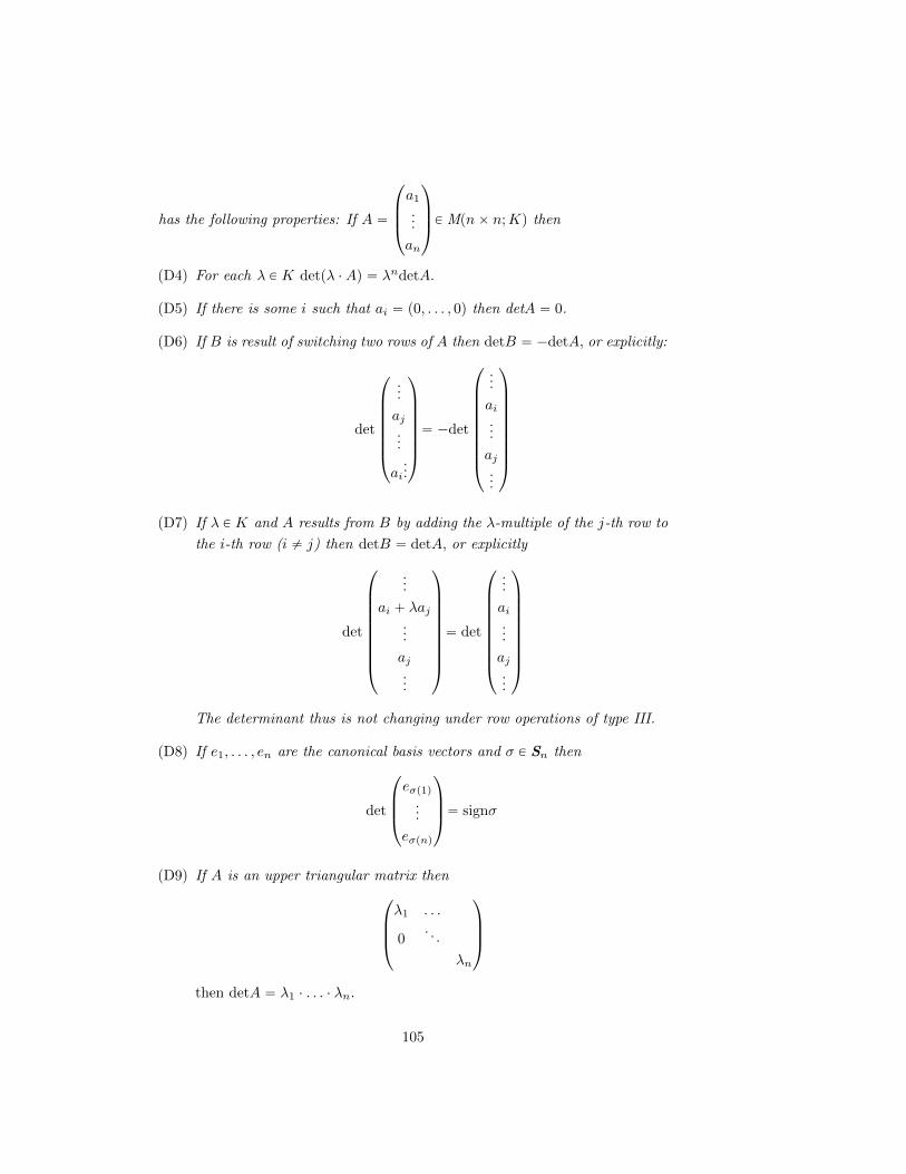
has the following properties: If A “

¨

˚

˚

˝

a1

...

an

˛

‹

‹

‚

P Mpnˆ n;Kq then

(D4) For each λ P K detpλ ¨Aq “ λndetA.

(D5) If there is some i such that ai “ p0, . . . , 0q then detA “ 0.

(D6) If B is result of switching two rows of A then detB “ ´detA, or explicitly:

det

¨

˚

˚

˚

˚

˚

˚

˝

...

aj...

ai...

˛

‹

‹

‹

‹

‹

‹

‚

“ ´det

¨

˚

˚

˚

˚

˚

˚

˚

˚

˝

...

ai...

aj...

˛

‹

‹

‹

‹

‹

‹

‹

‹

‚

(D7) If λ P K and A results from B by adding the λ-multiple of the j-th row to

the i-th row (i ‰ j) then detB “ detA, or explicitly

det

¨

˚

˚

˚

˚

˚

˚

˚

˚

˝

...

ai ` λaj...

aj...

˛

‹

‹

‹

‹

‹

‹

‹

‹

‚

“ det

¨

˚

˚

˚

˚

˚

˚

˚

˚

˝

...

ai...

aj...

˛

‹

‹

‹

‹

‹

‹

‹

‹

‚

The determinant thus is not changing under row operations of type III.

(D8) If e1, . . . , en are the canonical basis vectors and σ P Sn then

det

¨

˚

˚

˝

eσp1q...

eσpnq

˛

‹

‹

‚

“ signσ

(D9) If A is an upper triangular matrix then

¨

˚

˚

˝

λ1 . . .

0. . .

λn

˛

‹

‹

‚

then detA “ λ1 ¨ . . . ¨ λn.

105

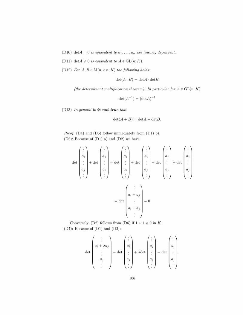
(D10) detA “ 0 is equivalent to a1, . . . , an are linearly dependent.

(D11) detA ‰ 0 is equivalent to A P GLpn;Kq.

(D12) For A,B P Mpnˆ n;Kq the following holds:

detpA ¨Bq “ detA ¨ detB

(the determinant multiplication theorem). In particular for A P GLpn;Kq

detpA´1q “ pdetAq´1

(D13) In general it is not true that

detpA`Bq “ detA` detB.

Proof. (D4) and (D5) follow immediately from (D1) b).

(D6): Because of (D1) a) and (D2) we have

det

¨

˚

˚

˚

˚

˚

˚

˚

˚

˝

...

ai...

aj...

˛

‹

‹

‹

‹

‹

‹

‹

‹

‚

` det

¨

˚

˚

˚

˚

˚

˚

˚

˚

˝

...

aj...

ai...

˛

‹

‹

‹

‹

‹

‹

‹

‹

‚

“ det

¨

˚

˚

˚

˚

˚

˚

˚

˚

˝

...

ai...

ai...

˛

‹

‹

‹

‹

‹

‹

‹

‹

‚

` det

¨

˚

˚

˚

˚

˚

˚

˚

˚

˝

...

ai...

aj...

˛

‹

‹

‹

‹

‹

‹

‹

‹

‚

` det

¨

˚

˚

˚

˚

˚

˚

˚

˚

˝

...

aj...

ai...

˛

‹

‹

‹

‹

‹

‹

‹

‹

‚

` det

¨

˚

˚

˚

˚

˚

˚

˚

˚

˝

...

aj...

aj...

˛

‹

‹

‹

‹

‹

‹

‹

‹

‚

“ det

¨

˚

˚

˚

˚

˚

˚

˚

˚

˝

...

ai ` aj...

ai ` aj...

˛

‹

‹

‹

‹

‹

‹

‹

‹

‚

“ 0

Conversely, (D2) follows from (D6) if 1` 1 ‰ 0 in K.

(D7): Because of (D1) and (D2):

det

¨

˚

˚

˚

˚

˚

˚

˚

˚

˝

...

ai ` λaj...

aj...

˛

‹

‹

‹

‹

‹

‹

‹

‹

‚

“ det

¨

˚

˚

˚

˚

˚

˚

˚

˚

˝

...

ai...

aj...

˛

‹

‹

‹

‹

‹

‹

‹

‹

‚

` λdet

¨

˚

˚

˚

˚

˚

˚

˚

˚

˝

...

aj...

aj...

˛

‹

‹

‹

‹

‹

‹

‹

‹

‚

“ det

¨

˚

˚

˚

˚

˚

˚

˚

˚

˝

...

ai...

aj...

˛

‹

‹

‹

‹

‹

‹

‹

‹

‚

.

106

(D8): If ρ P Sn is arbitrarily and τ P Sn is a transposition then by (D6):

det

¨

˚

˚

˝

eτpρp1qq...

eτpρpnqq

˛

‹

‹

‚

“ ´det

¨

˚

˚

˝

eρp1q...

eρpnq

˛

‹

‹

‚

.

For the given permutation σ we find by 4.1.3 transpositions τ1, . . . , τk such that

σ “ τ1 ˝ . . . ˝ τk,

and thus

det

¨

˚

˚

˝

eσp1q...

eσpnq

˛

‹

‹

‚

“ p´1qkdet

¨

˚

˚

˝

e1

...

en

˛

‹

‹

‚

“ p´1qkdetIn “ signσ

using (D3) and 4.1.9.

(D9): Let λi “ 0 for some i P t1, . . . , nu. By elementary row operations of type

III and IV we can transform A into a matrix

B “

¨

˚

˚

˚

˚

˚

˚

˚

˝

λ1 . . . .. . . . . .

0 λi´1 . .. . . .

0

˛

‹

‹

‹

‹

‹

‹

‹

‚

Since the last row of B is a zero row the determinant of B is 0 by (D5). On the

other hand by (D6) and (D7)

detA “ ˘detB.

Thus detA “ 0 and the claim has been proved. If λi ‰ 0 for all i P t1, . . . , nu

then by (D1) b)

detA “ λ1 ¨ λ2 ¨ . . . ¨ λn ¨ detB,

where B is of the form¨

˚

˚

˝

1 . . .

0. . .

1

˛

‹

‹

‚

and thus is an upper triangular matrix with all diagonal elements equal to 1.

Since it is possible to transform such a matrix by row operations of type III into

the identity matrix it follows that

detB “ detIn “ 1

107

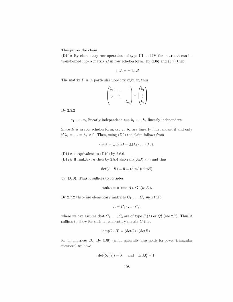
This proves the claim.

(D10): By elementary row operations of type III and IV the matrix A can be

transformed into a matrix B in row echelon form. By (D6) and (D7) then

detA “ ˘detB

The matrix B is in particular upper triangular, thus

¨

˚

˚

˝

λ1 . . .

0. . .

λn

˛

‹

‹

‚

“

¨

˚

˚

˝

b1...

bn

˛

‹

‹

‚

By 2.5.2

a1, . . . , an linearly independent ðñ b1, . . . , bn linearly independent.

Since B is in row echelon form, b1, . . . , bn are linearly independent if and only

if λ1 “ . . . “ λn ‰ 0. Then, using (D9) the claim follows from

detA “ ˘detB “ ˘pλ1 ¨ . . . ¨ λnq.

(D11): is equivalent to (D10) by 2.6.6.

(D12): If rankA ă n then by 2.8.4 also rankpABq ă n and thus

detpA ¨Bq “ 0 “ pdetAqpdetBq

by (D10). Thus it suffices to consider

rankA “ nðñ A P GLpn;Kq.

By 2.7.2 there are elementary matrices C1, . . . , Cs such that

A “ C1 ¨ . . . ¨ Cs,

where we can assume that C1, . . . , Cs are of type Sipλq or Qji (see 2.7). Thus it

suffices to show for such an elementary matrix C that

detpC ¨Bq “ pdetCq ¨ pdetBq.

for all matrices B. By (D9) (what naturally also holds for lower triangular

matrices) we have

detpSipλqq “ λ, and detQji “ 1.

108

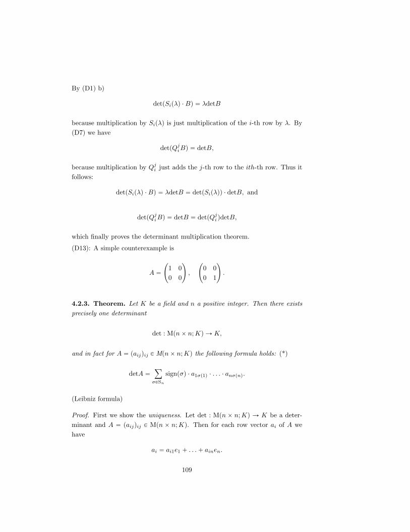
By (D1) b)

detpSipλq ¨Bq “ λdetB

because multiplication by Sipλq is just multiplication of the i-th row by λ. By

(D7) we have

detpQjiBq “ detB,

because multiplication by Qji just adds the j-th row to the ith-th row. Thus it

follows:

detpSipλq ¨Bq “ λdetB “ detpSipλqq ¨ detB, and

detpQjiBq “ detB “ detpQji qdetB,

which finally proves the determinant multiplication theorem.

(D13): A simple counterexample is

A “

˜

1 0

0 0

¸

,

˜

0 0

0 1

¸

.

4.2.3. Theorem. Let K be a field and n a positive integer. Then there exists

precisely one determinant

det : Mpnˆ n;Kq Ñ K,

and in fact for A “ paijqij P Mpnˆ n;Kq the following formula holds: (*)

detA “ÿ

σPSn

signpσq ¨ a1σp1q ¨ . . . ¨ anσpnq.

(Leibniz formula)

Proof. First we show the uniqueness. Let det : Mpn ˆ n;Kq Ñ K be a deter-

minant and A “ paijqij P Mpn ˆ n;Kq. Then for each row vector ai of A we

have

ai “ ai1e1 ` . . .` ainen.

109

Thus by repeated application of (D1) we get

det

¨

˚

˚

˝

a1

...

an

˛

‹

‹

‚

“

nÿ

i1“1

a1i1 ¨ det

¨

˚

˚

˚

˚

˝

ei1a2

...

an

˛

‹

‹

‹

‹

‚

“

nÿ

i1“1

a1i1 ¨

nÿ

i2“1

a2i2 ¨ det

¨

˚

˚

˚

˚

˝

ei1ei2a3

...an

˛

‹

‹

‹

‹

‚

“

nÿ

i1“1

nÿ

i2“1

. . .nÿ

in“1

a1i1 ¨ a2i2 ¨ . . . ¨ anin ¨ det

¨

˚

˚

˝

ei1...

ein

˛

‹

‹

‚

“ÿ

σPSn

a1σp1q ¨ a2σp2q ¨ . . . ¨ anσpnq ¨ det

¨

˚

˚

˝

eσp1q...

eσpnq

˛

‹

‹

‚

“ÿ

σPSn

signpσq ¨ a1σp1q ¨ . . . ¨ anσpnq

The equality before the last one follows from (D2) since

det

¨

˚

˚

˝

ei1...

ein

˛

‹

‹

‚

‰ 0

is equivalent to the existence of σ P Sn such that

i1 “ σp1q, . . . , in “ σpnq.

Thus among the a priori nn summands only n! are different from 0. The last

equation follows from (D8). This proves that the determinant has the form (*).

In order to prove existence we show that (*) defines a map


satisfying (D1), (D2) and (D3).

110

(D1) a):

det

¨

˚

˚

˚

˝

...

a1i ` a2i

...

˛

‹

‹

‹

‚

“ÿ

σPSn

signpσq ¨ a1σp1q ¨ . . . ¨ pa1iσpiq ` a

2iσpiqq ¨ . . . ¨ anσpnq

“ÿ

σPSn

signpσq ¨ a1σp1q ¨ . . . ¨ a1iσpiq ¨ . . . ¨ anσpnq

`ÿ

σPSn

signpσq ¨ a1σp1q ¨ . . . ¨ a2iσpiq ¨ . . . ¨ anσpnq

“ det

¨

˚

˚

˚

˝

...

a1i...

˛

‹

‹

‹

‚

`

¨

˚

˚

˚

˝

...

a2i...

˛

‹

‹

‹

‚

Similarly (D1) b) is checked by calculation.

(D2): Suppose that the k-th and `-th row of A are equal. Let k ă `. Let τ be

the transposition exchanging k and `. Then by 4.1.10

Sn “ An YAnτ,

and the union is disjoint. If σ P An then signσ “ `1 and signpσ ˝ τq “ ´1.

When σ runs through the elements of the group An then σ ˝ τ runs through the

lements of the set Anτ . Thus (**)

detA “ÿ

σPAn

a1σp1q ¨ . . . ¨ anσpnq ´ÿ

σPAn

a1σpτp1qq ¨ . . . ¨ anσpτpnqq.

Because the k-th and the `-th row of A are equal, by the very definition of τ

a1σpτp1qq ¨ . . . ¨ akσpτpkqq ¨ . . . ¨ a`σpτp`qq ¨ . . . ¨ anσpτpnqq

“ a1σp1q ¨ . . . ¨ akσp`q ¨ . . . ¨ a`σpkq ¨ . . . ¨ anσpnq

“ a1σp1q ¨ . . . akσpkq ¨ . . . ¨ a`σp`q ¨ . . . ¨ anσpnq

“ a1σp1q ¨ . . . ¨ anσpnq

Thus the two summands in (**) above cancel and detA “ 0 follows.

(D3): If δij is the Kronecker symbol and σ P Sn then

δ1σp1q ¨ . . . ¨ δnσpnq “

$

&

%

0 if σ ‰ id,

1 if σ “ id

Thus

detIn “ detpδijqijq “ÿ

σPSn

signpσq ¨ δ1σp1q ¨ . . . ¨ δnσpnq “ signpidq “ 1

111

˝

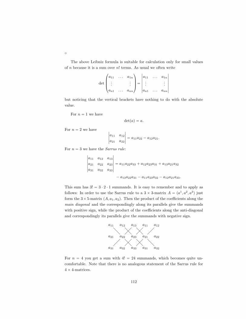
The above Leibniz formula is suitable for calculation only for small values

of n because it is a sum over n! terms. As usual we often write

det

¨

˚

˚

˝

a11 . . . a1n

......

an1 . . . ann

˛

‹

‹

‚

“

∣∣∣∣∣∣∣∣a11 . . . a1n

......

an1 . . . ann

∣∣∣∣∣∣∣∣but noticing that the vertical brackets have nothing to do with the absolute

value.

For n “ 1 we have

detpaq “ a.

For n “ 2 we have ∣∣∣∣∣a11 a12

a21 a22

∣∣∣∣∣ “ a11a22 ´ a12a21.

For n “ 3 we have the Sarrus rule:∣∣∣∣∣∣∣a11 a12 a13

a21 a22 a23

a31 a32 a33

∣∣∣∣∣∣∣ “ a11a22a33 ` a12a23a31 ` a13a21a32

´ a13a22a31 ´ a11a23a32 ´ a12a21a33.

This sum has 3! “ 3 ¨ 2 ¨ 1 summands. It is easy to remember and to apply as

follows: In order to use the Sarrus rule to a 3 ˆ 3-matrix A “ pa1, a2, a3q just

form the 3ˆ5-matrix pA, a1, a2q. Then the product of the coefficients along the

main diagonal and the correspondingly along its parallels give the summands

with positive sign, while the product of the coefficients along the anti-diagonal

and correspondingly its parallels give the summands with negative sign.

a11

a22

a12

a23

a13

a21

a31 a32 a33

a22

a32

a21

a11 a12

a31

For n “ 4 you get a sum with 4! “ 24 summands, which becomes quite un-

comfortable. Note that there is no analogous statement of the Sarrus rule for

4ˆ 4-matrices.

112

Until now we gave preference to row vectors in the definition of determinants.

We will see now that determinants have the same properties with respect to

column vectors.

4.2.4. Theorem. For each matrix A P Mpnˆ n;Kq the following holds:

detAT “ detA

Proof. Let A “ paijqij then AT “ pa1ijqij with a1ij “ aji. Then

detAT “ÿ

σPSn

signpσq ¨ a11σp1q ¨ . . . ¨ a1nσpnq

“ÿ

σPSn

signpσq ¨ aσp1q1 ¨ . . . ¨ aσpnqn

“ÿ

σPSn

signpσ´1qa1σ´1p1q ¨ . . . ¨ anσ´1pnq

“ detA

In the equation before the last one we used that for each σ P Sn

aσp1q1 ¨ . . . ¨ aσpnqn “ a1σ´1p1q ¨ . . . ¨ anσ´1pnq

because up to order the products contain the same factors. We also used

sign σ “ sign σ´1.

For the last equation we used that when σ runs through all permutations also

σ´1 does and vice versa, i. e. the map

Sn Ñ Sn, σ ÞÑ σ´1

is a bijection. This follows immediately from the uniqueness of the inverse of

some element in a group. ˝

4.3 Computation of determinants and some ap-

plications

Recall that if the square matrix B in row echelon form results from a square

matrix A by row operations of type III and IV then

detA “ p´1qkdetB

113

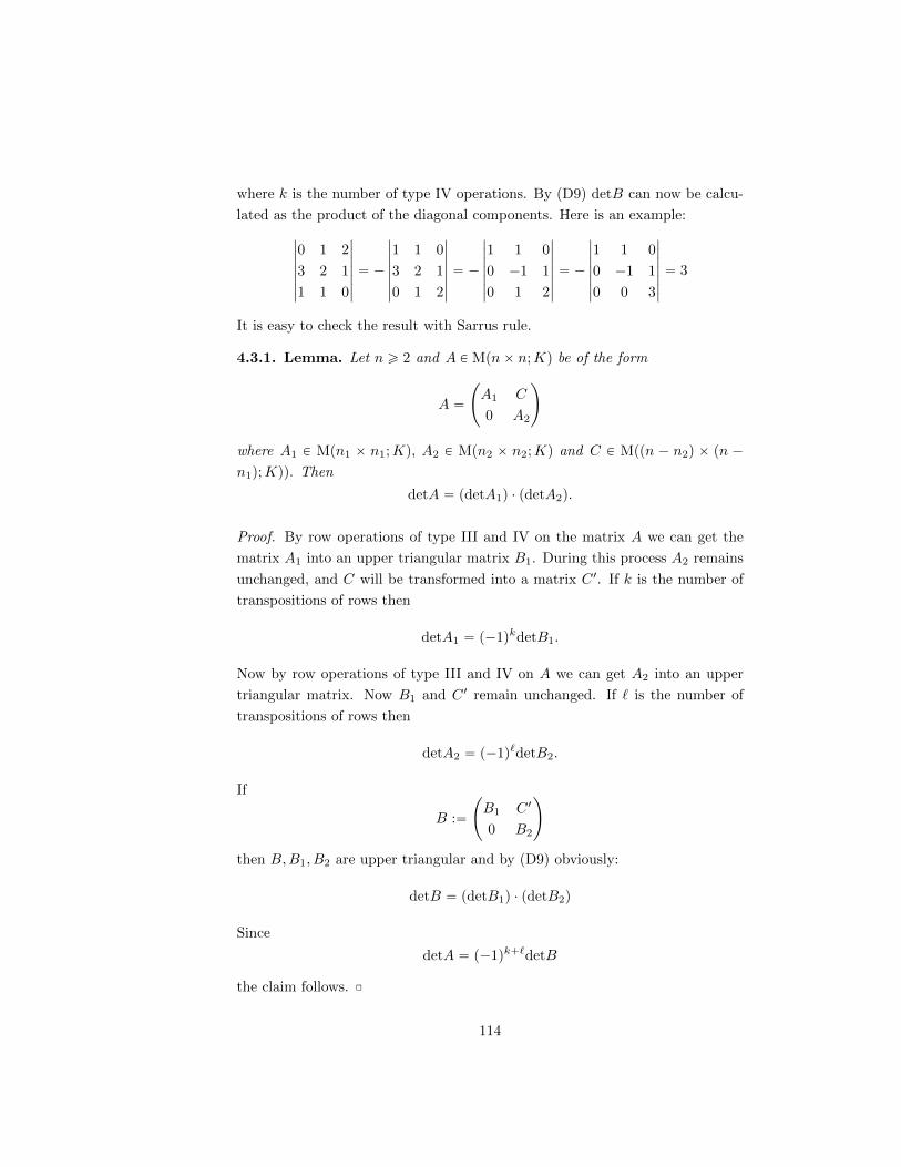
where k is the number of type IV operations. By (D9) detB can now be calcu-

lated as the product of the diagonal components. Here is an example:∣∣∣∣∣∣∣0 1 2

3 2 1

1 1 0

∣∣∣∣∣∣∣ “ ´∣∣∣∣∣∣∣1 1 0

3 2 1

0 1 2

∣∣∣∣∣∣∣ “ ´∣∣∣∣∣∣∣1 1 0

0 ´1 1

0 1 2

∣∣∣∣∣∣∣ “ ´∣∣∣∣∣∣∣1 1 0

0 ´1 1

0 0 3

∣∣∣∣∣∣∣ “ 3

It is easy to check the result with Sarrus rule.

4.3.1. Lemma. Let n ě 2 and A P Mpnˆ n;Kq be of the form

A “

˜

A1 C

0 A2

¸

where A1 P Mpn1 ˆ n1;Kq, A2 P Mpn2 ˆ n2;Kq and C P Mppn ´ n2q ˆ pn ´

n1q;Kqq. Then

detA “ pdetA1q ¨ pdetA2q.

Proof. By row operations of type III and IV on the matrix A we can get the

matrix A1 into an upper triangular matrix B1. During this process A2 remains

unchanged, and C will be transformed into a matrix C 1. If k is the number of

transpositions of rows then

detA1 “ p´1qkdetB1.

Now by row operations of type III and IV on A we can get A2 into an upper

triangular matrix. Now B1 and C 1 remain unchanged. If ` is the number of

transpositions of rows then

detA2 “ p´1q`detB2.

If

B :“

˜

B1 C 1

0 B2

¸

then B,B1, B2 are upper triangular and by (D9) obviously:

detB “ pdetB1q ¨ pdetB2q

Since

detA “ p´1qk``detB

the claim follows. ˝

114

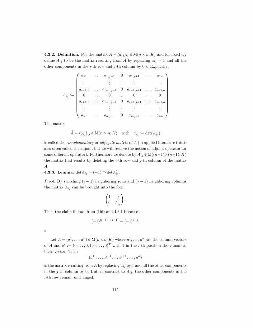
4.3.2. Definition. For the matrix A “ paijqij P Mpnˆ n;Kq and for fixed i, j

define Aij to be the matrix resulting from A by replacing aij “ 1 and all the

other components in the i-th row and j-th column by 0’s. Explicitly:

Aij :“

¨

˚

˚

˚

˚

˚

˚

˚

˚

˚

˚

˚

˚

˝

a11 . . . a1,j´1 0 a1,j`1 . . . a1n

......

......

...

ai´1,1 . . . ai´1,j´1 0 ai´1,j`1 . . . ai´1,n

0 . . . 0 1 0 . . . 0

ai`1,1 . . . ai`1,j´1 0 ai`1,j`1 . . . ai`1,n

......

......

...

an1 . . . an,j´1 0 an,j`1 . . . ann

˛

‹

‹

‹

‹

‹

‹

‹

‹

‹

‹

‹

‹

‚

The matrix

A “ paijqij P Mpnˆ n;Kq with aij :“ detpAjiq

is called the complementary or adjugate matrix of A (in applied literature this is

also often called the adjoint but we will reserve the notion of adjoint operator for

some different operator). Furthermore we denote by A1ij P Mppn´1qˆpn´1q;Kq

the matrix that results by deleting the i-th row and j-th column of the matrix

A.

4.3.3. Lemma. detAij “ p´1qi`jdetA1ij .

Proof. By switching pi ´ 1q neighboring rows and pj ´ 1q neighboring columns

the matrix Aij can be brought into the form

˜

1 0

0 A1ij

¸

.

Then the claim follows from (D6) and 4.3.1 because

p´1qpi´1q`pj´1q “ p´1qi`j .

˝

Let A “ pa1, . . . , anq P Mpnˆn;Kq where a1, . . . , an are the column vectors

of A and ei :“ p0, . . . , 0, 1, 0, . . . , 0qT with 1 in the i-th position the canonical

basis vector. Then

pa1, . . . , aj´1, ei, aj`1, . . . , anq

is the matrix resulting from A by replacing aij by 1 and all the other components

in the j-th column by 0. But, in contrast to Aij , the other components in the

i-th row remain unchanged.

115

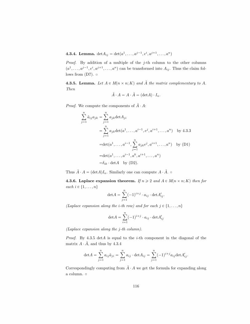
4.3.4. Lemma. detAij “ detpa1, . . . , aj´1, ei, aj`1, . . . , anq

Proof. By addition of a multiple of the j-th column to the other columns

pa1, . . . , aj´1, ei, aj`1, . . . , anq can be transformed into Aij . Thus the claim fol-

lows from (D7). ˝

4.3.5. Lemma. Let A P Mpn ˆ n;Kq and A the matrix complementary to A.

Then

A Ä “ A ¨ A “ pdetAq ¨ In.

Proof. We compute the components of A Ä:

nÿ

j“1

aijajk “nÿ

j“1

ajkdetAji

“

nÿ

j“1

ajkdetpa1, . . . , ai´1, ej , ai`1, . . . , anq by 4.3.3

“detpa1, . . . , ai´1,nÿ

j“1

ajkej , ai`1, . . . , anq by (D1)

“detpa1, . . . , ai´1, ak, ai`1, . . . , anq

“δik ¨ detA by (D2).

Thus A Ä “ pdetAqIn. Similarly one can compute A ¨ A. ˝

4.3.6. Laplace expansion theorem. If n ě 2 and A P Mpnˆ n;Kq then for

each i P t1, . . . , nu

detA “nÿ

j“1

p´1qi`j ¨ aij ¨ detA1ij .

(Laplace expansion along the i-th row) and for each j P t1, . . . , nu

detA “nÿ

i“1

p´1qi`j ¨ aij ¨ detA1ij

(Laplace expansion along the j-th column).

Proof. By 4.3.5 detA is equal to the i-th component in the diagonal of the

matrix A ¨ A, and thus by 4.3.4

detA “nÿ

j“1

aij aji “nÿ

j“1

aij ¨ detAij “nÿ

j“1

p´1qi`jaijdetA1ij .

Correspondingly computing from A Ä we get the formula for expanding along

a column. ˝

116

Essentially the Laplace expansion formula is just a method to write the sum

in the Leibniz expansion 4.2.3 in a special series of terms. But of course this is

comfortable if there are many zero entries in a row or column. Of course the

computational rules for determinants from the beginning of this section can be

combined with Laplace expansion.

Here is a simple example:∣∣∣∣∣∣∣0 1 2

3 2 1

1 1 0

∣∣∣∣∣∣∣ “ 0 ¨

∣∣∣∣∣2 1

1 0

∣∣∣∣∣´ 1 ¨

∣∣∣∣∣3 1

1 0

∣∣∣∣∣` 2 ¨

∣∣∣∣∣3 2

1 1

∣∣∣∣∣ “ 0 ¨ p´1q ´ 1 ¨ p´1q ` 2 ¨ 1 “ 3

The sign distributions generated by the factor p´1qi`j can be thought of as a

chess board coloring:

+ - + - + - + -

- + - + - + - +

+ - + - + - + -

- + - + - + - +

+ - + - + - + -

- + - + - + - +

+ - + - + - + -

- + - + - + - +

From 4.3.5 we can get immediately a method to calculate the inverse of a

matrix using determinants. Let A1ij be the matrix defined above by deleting the

i-th row and j-th column. Let A P GLpn;Kq. Define C “ pcijqij P Mpnˆ n;Kq

be defined by

cij :“ p´1qi`j ¨ detA1ij .

Then

A´1 “1

detpAq¨ CT .

In the special case n “ 2 we get˜

a b

c d

¸´1

“1

ad´ bc

˜

d ´c

´b a

¸T

“1

ad´ bc

˜

d ´b

´c a

¸

The method is still of practical interest for p3 ˆ 3q-matrices but get unwieldy

for matrices of larger size.

We would like to mention an important consequence of the previous result.

If we identify Mpnˆ n;Rq with Rn2

then we get the differentiable function

det : Rn2

Ñ R.

117

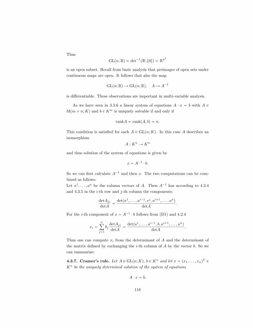
Thus

GLpn;Rq “ det´1pRzt0uq Ă Rn

2

is an open subset. Recall from basic analysis that preimages of open sets under

continuous maps are open. It follows that also the map

GLpn;Rq Ñ GLpn;Rq, A ÞÑ A´1

is differentiable. These observations are important in multi-variable analysis.

As we have seen in 3.3.6 a linear system of equations A ¨ x “ b with A P

Mpmˆ n;Kq and b P Km is uniquely solvable if and only if

rankA “ rankpA, bq “ n.

This condition is satisfied for each A P GLpn;Kq. In this case A describes an

isomorphism

A : Kn Ñ Kn

and thus solution of the system of equations is given by

x “ A´1 ¨ b.

So we can first calculate A´1 and then x. The two computations can be com-

bined as follows:

Let a1, . . . , an be the column vectors of A. Then A´1 has according to 4.3.4

and 4.3.5 in the i-th row and j-th column the components:

detAjidetA

“detpa1, . . . , ai´1, ej , ai`1, . . . , anq

detA.

For the i-th component of x “ A´1 ¨ b follows from (D1) and 4.2.4

xi “nÿ

j“1

bjdetAjidetA

“detpa1, . . . , ai´1, b, ai`1, . . . , anq

detA.

Thus one can compute xi from the determinant of A and the determinant of

the matrix defined by exchanging the i-th column of A by the vector b. So we

can summarize:

4.3.7. Cramer’s rule. Let A P GLpn;Kq, b P Kn and let x “ px1, . . . , xnqT P

Kn be the uniquely determined solution of the system of equations

A ¨ x “ b.

118

Let a1, . . . , an be the column vectors of A. Then for each i P t1, . . . , nu

xi “detpa1, . . . , ai´1, b, ai`1, . . . , anq

detA

˝

For large n Cramer’s rule is not a practical method because we have to

compute n`1 determinants. For theoretical considerations though Cramer’s rule

is valuable. For example for K “ R it is possible to see easily that the solution

x of a system of equations Ax “ b depends continuously on the coefficients of

both A and b.

For examples see e. g.

http://www.okc.cc.ok.us/maustin/Cramers_Rule/Cramer’s%20Rule.htm

As a last application of determinants we discuss an often applied method

to determine the rank of a matrix. Let A P Mpm ˆ n;Kq and k ď mintm,nu.

Then a quadratic matrix A1 P Mpk ˆ k;Kq is called a k-row sub-matrix of A if

A can be brought by permutations of rows and permutations of columns into

the form˜

A1 ˚

˚ ˚

¸

where ˚ denotes any matrices.

4.3.8. Theorem. Let A P Mpm ˆ n;Kq and r P N. Then the following

conditions are equivalent:

i) r “ rankA.

ii) There exists an r-row sub-matrix A1 of A such that detA1 ‰ 0, and if k ą r

then for each k-row sub-matrix of A it follows that detA1 “ 0.

It suffices to show that for each k P N the following two conditions are

equivalent:

a) rankA ě k.

b) There exists a k-row sub-matrix A1 of A such that detA1 ‰ 0.

b)ùñ a): From detA1 ‰ 0 it follows rankA1 ě k thus also rankA ě k because

the rank of a matrix is not changing under permutations of rows or columns.

a) ùñ b): Let rankA ě k then there are k linearly independent row vectors in

A. After permuting rows we can assume that they are the first k rows. Let B

be the matrix consisting of those rows. Since

row-rankB “ k “ col-rankB

119

http://www.okc.cc.ok.us/maustin/Cramers_Rule/Cramer's%20Rule.htm

there are k linearly independent column vectors in B. By permuting columns

we can assume those are the first k columns of B. Let A1 P Mpk ˆ k;Kq be

the matrix consisting of these columns. Then A1 is a sub-matrix of A and since

rankA1 “ k it follows detA1 ‰ 0. This proves the result. ˝

4.4 The determinant of an endomorphism, ori-

entation

Let V be a K-vector space of dimension n ă 8. We will define a map:

det : LKpV q Ñ K

Let A be an arbitrary basis of V and F P LKpV q. Then we set

detF :“ detMApF q,

i. e. the determinant of a representing matrix. We have to prove that this does

not depend on choice of A. If B is another basis then by the transformation

formula from 2.8n there exists a matrix S P GLpm;Kq such that

MBpF q “ S ¨MApF q ¨ S´1.

By the determinant multiplication theorem from 4.2 it follows that

detMBpF q “ pdetSq ¨ detMApF q ¨ pdetSq´1 “ detMApF q.

4.4.1. Remark. For each endomorphism F P LKpV q the following are equiva-

lent:

(i) F is surjective.

(ii) detF ‰ 0

Proof. If A is a representing matrix of A then

rankA “ rankF and detA “ detF.

By (D11) we know that rankA “ n is equivalent to detA ‰ 0. This proves the

claim. ˝

In the case V “ Rn the determinant of an endomorphism has an important

geometric interpretation. Let pv1, . . . , vnq P Rn and let A be the matrix with

120

column vectors ai. Then it is shown in analysis that |detA| is the volume of the

parallelotope (generalization of parallelepiped) spanned by v1, . . . , vn (see

http://www.scribd.com/doc/76916244/15/Parallelotope-volume

for an introduction). The canonical basis vectors span the unit cube of volume

1 in Rn. Now if F : Rn Ñ Rn is an endomorphism and A is the matrix

representing F with respect to the canonical basis then

|detA| “ |detF |

the volume of the paralellotope spanned by F pe1q, . . . , F penq (it is the image of

the unit cube under the endomorphism F ). Thus |detF is the volume distortion

due to F .

Let V be an R-vector space with 1 ď dimV ă 8. Then an endomorphism

is called orientation preserving if

detF ą 0.

Note that it follows that F is actually an automorphism. If detF ă 0 then F is

called orientation reversing.

4.4.2. Example. Consider automorphisms of R2. The identity map is orienta-

tion preserving. It will map the letter F to itself. A reflection about the y-axis

will map the letter F to the letter F, and this is orientation reversing.

The notion of orientation itself is slightly more difficult to explain:

4.4.3. Definition. Let A and B be two bases of V . Then there is precisely one

automorphism F : V Ñ V such that F pviq “ wi for i “ 1, . . . , n. We say that

A and B have the same orientation, denoted by A „ B if detF ą 0. Otherwise

A and B are called oppositely oriented or have opposite orientation.

Using the determinant multiplication theorem it follows immediately that „

defines an equivalence relation on the set M of all bases of V , decomposing M

into two disjoint equivalence classes

M “M1 YM2,

where any two bases in Mi have the same orientation. The two sets M1,M2 are

called the orientations of V . An orientation is just an equivalence class of bases

having the same orientation.

It is important to note that there are precisely two possible orientations and

none of it is distinguished.

121

http://www.scribd.com/doc/76916244/15/Parallelotope-volume

Recall the definition of the vector product of two vectors x “ px1, x2, x3q

and y “ py1, y2, y3q in R3:

xˆ y :“ px2y3 ´ x3y2, x3y1 ´ x1y3, x1y2 ´ x2y1q P R3.

4.4.4. Proposition. If x, y P R3 are linearly independent then the bases

pe1, e2, e3q and x, y, xˆ y have the same orientation.

Proof. We have

xˆ y “

˜∣∣∣∣∣x2 y2

x3 y3

∣∣∣∣∣ ,´∣∣∣∣∣x1 y1

x3 y3

∣∣∣∣∣ ,∣∣∣∣∣x1 y1

x2 y2

∣∣∣∣∣¸

“: pz1, z2, z3q

If we expand along the third column we get∣∣∣∣∣∣∣x1 y1 z1

x2 y2 z2

x3 y3 z3

∣∣∣∣∣∣∣ “ z21 ` z

22 ` z

23 ą 0.

In fact xˆ y ‰ 0 follows from linear independence of x and y (Exercise!).

4.4.5. Proposition. Let pv1, . . . , vnq be a basis of Rn and σ P Sn. Then the

following are equivalent:

(i) pv1, . . . , vnq and pvσp1q, . . . , vσpnqq have the same orientation.

(ii) sign σ “ `1.

˝

The geometric background of the notion of orientation is of topological na-

ture. We want to see that two bases have the same orientation if and only if they

can be continuously deformed into each other. For each basis A “ pv1, . . . , vnq

be a basis of Rn there is defined the matrix invertible A with column vectors

v1, . . . , vn. Thus we have a map

M Ñ GLpn;Rq, A ÞÑ A,

where M is the set of bases of Rn. This map is obviously bijective. Furthermore

there is a bijective map

Mpnˆ n;Rq Ñ Rn2

,

which allows to consider GLpn;Rq as a subset of Rn2

. Because of the continuity

of the determinant:

GLpn;Rq “ tA P Mpnˆ n;Rq : detA ‰ 0u

122

is an open subset of Rn2

. Thus for simplicity we will not distinguish between

M and GLpn;Rq and consider both as subsets of Rn2

.

4.4.6. Definition. Let A,B P GLpn;Rq. Then A is continuously deformable

into B if there is a closed interval I “ ra, bs Ă R and a continuous map

ϕ : I Ñ GLpn;Rq

such that ϕpaq “ A and ϕpBq “ B.

Continuity of ϕ means that the n2 component of ϕ are continuous real valued

functions. Thus deformable means that we can get the components of B by

continuously deforming the components of A. Essential though is that during

the deformation the matrix at each point in time has to be invertible (otherwise

we can deform any two matrices into each other, why?).

Deformability defines an equivalence relation on GLpn;Rq.

4.4.7. Lemma. Let A P GLpn;Rq be given. Then the following are equivalent:

(i) detA ą 0.

(ii) A is continuously deformable into the identity matrix In.

Proof. (ii) ùñ (i) follows by purely topological reasons. If ϕ : I Ñ GLpn;Rqwith ϕpaq “ A and ϕpbq “ In then we consider the composite map

IϕÝÑ GLpn;Rq det

ÝÑ R˚,

which is continuous because of the continuity of ϕ and det. It follows from the

intermediate value theorem and detIn “ 1 that detA ą 0 (because otherwise

there exists τ P r0, 1s such that detpϕpτqq “ 0, which contradicts that the target

of det ˝ϕ in Rzt0u. (i) ùñ (ii) is more difficult. First we note that the identity

matrix In can be continuously deformed into any of the elementary matrices:

Sipλq “ In ` pλ´ 1qEii with λ ą 0 and

Qji pµq “ In ` µEji with i ‰ j and arbitrary µ P R.

The necessary continuous maps in this case are

(*) ϕ : r0, 1s Ñ GLpn;Rq, t ÞÑ In ` t ¨ pλ´ 1qEii

(**) ψ : r0, 1s Ñ GLpn;Rq, t ÞÑ In ` t ¨ µEji .

123

Continuity of ϕ and ψ are immediate from the continuity of the addition and

multiplication operations in R. The given matrix A with detA ą 0 now can be

transformed into a diagonal matrix D by row operations of type III. So there

are elementary matrices of type III such that

D “ Bk ¨ . . . ¨B1 Ä.

If for exampleB “ Qji pµq and ψ is defined by (**) then we consider the composed

map

r0, 1sψÝÑ GLpn;Rq α

ÝÑ GLpn;Rq,

where α is defined by

αpBq :“ B Ä for all B P GLpn;Rq.

Since α is continuous also α ˝ ψ is continuous, and because

pα ˝ ψqp0q “ A, pα ˝ ψqp1q “ Qji pµq Ä

we have continuously deformed the matrix A into the matrix B1 Ä. Since

detpB1 Äq “ detA ą 0

this process can be repeated, and finally we have deformed the matrix A into

the diagonal matrix D. By multiplying the rows of D by positive real numbers

we can finally transform the matrix D into a diagonal matrix D1 with diagonal

components all ˘1. There are corresponding elementary matrices C1, . . . , Cl of

type I with detCi ą 0 for i “ 1, . . . , l such that

D1 “ Cl ¨ . . . ¨ C1 ¨D.

In an analogous way using the map ϕ from (*) above we see that D can be

deformed into D1. In the last step we show that D1 can be deformed continuously

into In. Since

1 “ detD1 ą 0

there are an even number of ´1’s on the diagonal. We first consider in the

special case n “ 2 the matrix

D1 “

˜

´1 0

0 ´1

¸

P GLp2;Rq

and the continuous map

α : r´π, 0s Ñ GLp2,Rq, t ÞÑ

˜

cos t ´ sin t

sin t cos t

¸

124

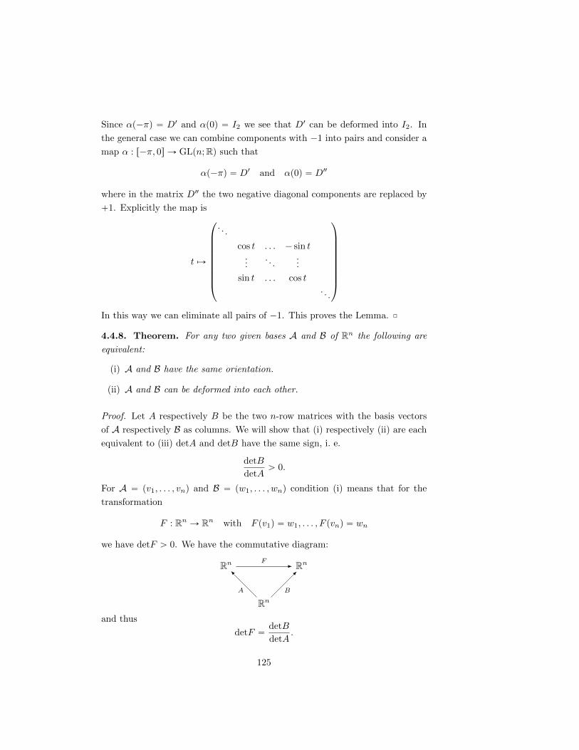
Since αp´πq “ D1 and αp0q “ I2 we see that D1 can be deformed into I2. In

the general case we can combine components with ´1 into pairs and consider a

map α : r´π, 0s Ñ GLpn;Rq such that

αp´πq “ D1 and αp0q “ D2

where in the matrix D2 the two negative diagonal components are replaced by

`1. Explicitly the map is

t ÞÑ

¨

˚

˚

˚

˚

˚

˚

˚

˚

˝

. . .

cos t . . . ´ sin t...

. . ....

sin t . . . cos t. . .

˛

‹

‹

‹

‹

‹

‹

‹

‹

‚

In this way we can eliminate all pairs of ´1. This proves the Lemma. ˝

4.4.8. Theorem. For any two given bases A and B of Rn the following are

equivalent:

(i) A and B have the same orientation.

(ii) A and B can be deformed into each other.

Proof. Let A respectively B be the two n-row matrices with the basis vectors

of A respectively B as columns. We will show that (i) respectively (ii) are each

equivalent to (iii) detA and detB have the same sign, i. e.

detB

detAą 0.

For A “ pv1, . . . , vnq and B “ pw1, . . . , wnq condition (i) means that for the

transformation

F : Rn Ñ Rn with F pv1q “ w1, . . . , F pvnq “ wn

we have detF ą 0. We have the commutative diagram:

Rn F - Rn

RnB

-

A

�

and thus

detF “detB

detA.

125

Thus (i) is equivalent to (iii). In order to show the equivalence of (ii) and (iii)

consider the map

Φ : GLpn;Rq Ñ GLpn;Rq, C ÞÑ C 1,

where C 1 results from C by multiplying the first column by ´1. The resulting

map Φ is obviously bijective (with inverse Φ itself), and Φ is continuous. Since

detC 1 “ ´detC

it follows from the Lemma that

detA ă 0

is equivalent to the fact that A can be continuously deformed into I 1n. Thus

A and B can be continuously deformed into each other if both can be either

deformed into In or both can be deformed into I 1n, i. e. if detA and detB have the

same sign. It follows from the intermediate value theorem that this condition is

also necessary. ˝

4.4.9. Remarks. (i) It follows from the above that the group GLpn;Rq has

precisely two components, namely:

tA P GLpn;Rq : detA ą 0u and tA P GLpn;Rq : detA ă 0u

See the wiki page

http://en.wikipedia.org/wiki/Connected_space

for the notion of connected components and path components.

(ii) It can be proven using the above methods that the group GLpn;Cq is con-

nected, i. e. any two complex invertible matrices can be deformed into each other

through invertible complex matrices. The reason for this is that each complex

number in C˚ “ Czt0u can be joined with 1 P C˚ by a continuous path.

126

http://en.wikipedia.org/wiki/Connected_space

Chapter 5

Eigenvalues,

Diagonalization and

Triangulation of

Endomorphisms

In 2.8 we have proven that for each linear transformation

F : V ÑW

between finite dimensional K-vector spaces we can find bases A of V and B of

W such that

MAB pF q “

˜

Ir 0

0 0

¸

where r “ rankF . For endomorphisms F : V Ñ V it seems to be useful to

consider only one basis of the vector space, i. e. A “ B. We thus will consider

the problem to find just one basis B of V such that

MBpF q

has particularly simple form.

127

5.1 Similarity of matrices, Eigenvalues, Eigen-

vectors

5.1.1. Definition. Two matrices A,B P Mpnˆn;Kq are called similar if there

exists S P GLpn;Kq such that

B “ SAS´1.

Because of the transformation formula in 2.8 this is equivalent to the asser-

tion that there exists an n-dimensional vector space V and an endomorphism

F : V Ñ V and bases A and B such that

A “MApF q and B “MBpF q.

It is easy to show that similarity of matrices defines an equivalence relation.

So our question is whether it is possible to choose in each equivalence class a

particularly simple representative, usually called a normal form.

Consider first V “ R. For each endomorphism F : R Ñ R we have F pvq “

λ ¨ v with λ :“ F p1q. Thus F is represented with respect to all bases by the

1ˆ1-matrix pλq. The number λ is characteristic for F . This leads in the general

case to the following:

5.1.2. Definition. Let F be an endomorphism of the K-vector space V . A

scalar λ P K is called an eigenvalue of F if there exists a vector 0 ‰ v P V such

that F pvq “ λv. Each vector v ‰ 0 such that F pvq “ λv is called an eigenvector

of F (for the eigenvalue λ).

Note that 0 P K can be an eigenvalue while 0 P V is not an eigenvector.

5.1.3. Proposition. Let dimV ă 8. Then the following are equivalent:

(i) There exists a basis of V consisting of eigenvectors of F .

(ii) There exists a basis B of V such that MBpF q is a diagonal matrix, i. e.

MBpF q “ Dpλ1, . . . , λnq “

¨

˚

˚

˝

λ1

0. . . 0

λn

˛

‹

‹

‚

“: diagpλ1, . . . , λnq

Proof. Let B “ pv1, . . . , vnq be a basis of V . Then the columns of MBpF q are the

coordinate vectors of F pv1q, . . . , F pvnq with respect to v1, . . . , vn. This proves

the claim. ˝

128

An endomorphism F : V Ñ V is called diagonalizable if one of the two

equivalent conditions in 5.1.3 is satisfied. In particular, a matrix A P Mpnˆn;Kq

is called diagonalizable if the endomorphism A : Kn Ñ Kn represented by the

matrix is diagonalizable. This condition is equivalent to the assertion that A is

similar to a diagonal matrix.

Note that, even if F is diagonalizable then not necessarily each vector v P V

is an eigenvector!

For the description of endomorphisms by matrices a basis consisting of eigen-

vectors thus gives most simplicity. Unfortunately, as we will see, such a basis

will not exist in general.

5.1.4. Lemma. If v1, . . . , vm are eigenvectors for pairwise distinct eigenvalues

λ1, . . . , λm of F P LKpV q then v1, . . . , vm are linearly independent. Thus, in

particular if dimV “ n ă 8 and F has pairwise distinct eigenvalues λ1, . . . , λn

then F is diagonalizable.

Proof. The proof is by induction on m. The case m “ 1 is clear because v1 ‰ 0.

Let m ě 2 and the claim proved for m´ 1. Let

α1v1 ` . . . αmvm “ 0

with α1, . . . , αm P K. It follows that

0 “λm0 “ λmα1v1 ` . . .` λmαmvm and

0 “F p0q “ λ1α1v1 ` . . .` λmαmvm, thus

0 “α1pλm ´ λ1qv1 ` . . .` αm´1pλm ´ λm´1qvm´1.

Now by application of the induction hypothesis to v1, . . . , vm´1 we get that

v1, . . . , vm´1 are linearly independent. Because λm´λ1 ‰ 0, . . . , λm´λm´1 ‰ 0

it follows that α1 “ . . . “ αm´1 “ 0 and finally also αm “ 0 because vm ‰ 0. ˝

In order to apply 5.1.4 we have to know the eigenvalues. This will be the

subject of the next section.

5.2 The characteristic polynomial

Let V be K-vector space.

5.2.1. Definition. For F P LKpV q and λ P K let

EigpF ;λq :“ tv P V : F pvq “ λvu

129

be the eigenspace of F with respect to λ.

5.2.2. Remarks. (a) EigpF ;λq Ă V is a subspace.

(b) λ is eigenvalue of F ðñ EigpF ;λq ‰ t0u.

(c) EigpF ;λqzt0u is the set of eigenvectors of F with respect to λ P K.

(d) EigpF ;λq “ kerpF ´ λidV q.

(e) If λ1, λ2 P K and λ1 ‰ λ2 then

EigpF ;λ1q X EigpF ;λ2q “ t0u.

Proof. (a)-(d) is clear. (e) follows because if F pvq “ λ1v and F pvq “ λ2v then

pλ1 ´ λ2qv “ 0 and thus v “ 0. ˝

Given F and λ properties (b) and (d) can be used to decide whether λ is an

eigenvalue.

5.2.3. Lemma. Let dimV ă 8. Then for F P LKpV q and λ P K the following

are equivalent:

(i) λ is an eigenvalue of F .

(ii) detpF ´ λidV q “ 0.

Proof. By 5.2.2 we have

λ is an eigenvalue of F ðñ detpF ´ λidV q “ 0.

This proves the claim. ˝

Let F P LKpV q and A be a basis of V . If dimV “ n ă 8 and if

A “MApF q, then MApF ´ λidV q “ A´ λIn

for each λ P K. Instead of λ we introduce a parameter t and define

PF “ detpA´ t ¨ Inq “

∣∣∣∣∣∣∣∣∣∣a11 ´ t a12 . . . a1n

a21 a22 ´ t . . . a2n

......

...

an1 an2 . . . ann ´ t

∣∣∣∣∣∣∣∣∣∣Note that we consider the matrix A´ t ¨ In as an element of Mpnˆ n;Krtsq

and apply then formula 4.2.3 to calculate the determinant formally applying

the formula in 4.2.3. In the calculations often the formal rules (most but not all

130

of (D1)-(D12) will work!). Thus actually we are calculating the determinant of

a matrix with entries in the commutative unital ring Krts. Interestingly we can

also consider A´ t ¨ In as an element in Rrts where R “ Mpnˆ n;Kq (Check in

which sense Rrts “ Mpnˆ n;Krtsq).

Using 4.2.3 to calculate the determinant we get:

PF “ pa11 ´ tqpa22 ´ tq ¨ . . . ¨ pann ´ tq `Q

where the first summand corresponds to the identity permutation and Q denotes

the remaining sum over Snztidu. Because in each factor of Q there can be at

most n ´ 2 diagonal components, Q is a polynomial of degree at most n ´ 2.

Now

pa11 ´ tq ¨ . . . ¨ pann ´ tq “ p´1qntn ` p´1qn´1pa11 ` . . .` annqtn´1 `Q1,

where Q1 is a polynomial of degree at most n´ 2. Thus PF is a polynomial of

degree n with coefficients in K, i. e. there are α0, . . . , αn P K such that

PF “ αntn ` αn´1t

n´1 ` . . .` α1t` α0.

In fact we know that

α0 “p´1qn

αn´1 “p´1qn´1pa11 ` . . .` annq and

αn “detA

Here a11 ` . . . ` ann is the trace of A and has been defined in the Homework

Problem 26. The coefficients α1, . . . , αn´2 are not that easy to describe and

thus have no special names. The polynomial PF is called the characteristic

polynomial of F . This makes sense because PF does not depend on the choice

of the basis A.

5.2.4. Definition. For A P Mpnˆ n;Kq the polynomial

PA :“ detpA´ t ¨ Inq P Krts

is called the characteristic polynomial of A. (This definition is due to A. L.

Cauchy.)

5.2.5. Lemma. Let A,B P Mpnˆ n;Kq be similar matrices. Then PA “ PB.

Proof. Let B “ SAS´1 with S P GLpn;Kq. Then

S ¨ t ¨ In ¨ S´1 “ t ¨ In.

131

This calculation is actually happening in the polynomial ring Rrts where R “

Mpnˆ n;Kq (see the Remark following 5.2.3). Also

B ´ t ¨ In “ SAS´1 ´ S ¨ t ¨ InS´1 “ SpA´ t ¨ InqS

´1,

and thus by application of the determinant

detpB ´ t ¨ Inq “ detS ¨ detpA´ t ¨ Inq ¨ pdetSq´1 “ detpA´ t ¨ Inq.

This proves the claim. ˝

In the proof of 5.2.5 we computed by interpreting A ´ t ¨ In as an element

in Rrts for R “ Mpn ˆ n;Kq while the definition of the determinant is based

on interpreting it as element of Mpnˆ n;Krtsq, we already indicated this point

above. We can avoid this tricky part in the case when we know that the linear

transformation:

Krts Ñ MappK,Kq,

which assigns to each polynomial the corresponding polynomial function is in-

jective. We will show in the Intermezzo below that this is the case if the field

K is infinite, i. e. in particular for K “ Q,R or C. In fact equality of the cor-

responding polynomial functions is easy because we only have to work over K:

For each λ P K we have

PBpλq “ detpB ´ λInq “detpSAS´1 ´ λSInS´1q

“detpSpA´ λInqS´1q

“detS ¨ detpA´ λInq ¨ pdetSq´1

5.2.6. Remark. The definition of the characteristic polynomial of an endo-

morphism in 5.2.4 does not depend on the choice of basis.

Proof. If F P LKpV q and A, B are two bases of V then by the transformation

formula from 2.8 there exists S P GLpn;Kq such that

MBpF q “ SMApF qS´1.

The claim follows from 5.2.5. ˝

We first summarize our results in the following theorem. If P “ a0 ` a1t`

. . .` antn P Krts then we call λ P K a zero (or root) of P if

P pλq “ a0 ` a1λ` . . .` anλn “ 0 P K.

132

5.2.7. Theorem. Let V be a K-vector space of dimension n ă 8 and let

F P LKpV q. Then there exists a uniquely determined characteristic polynomial

PF P Krts with the following properties:

(a) degPF “ n.

(b) If A is a matrix representing the endomorphism F then

PF “ detpA´ t ¨ Inq

.

(c) PF describes the mapping

K Ñ K, λ ÞÑ detpF ´ λidq.

(d) The zeros of PF are the eigenvalues of F . ˝

Intermezzo on polynomials and polynomial functions.

We want to prove the claim mentioned above namely, that for K an infinite

field the linear transformation

Krts Ñ MappK,Kq, P ÞÑ P

is injective. Because of linearity this is equivalent to P “ 0 ùñ P “ 0. The

claim will follow from I.1 below because if we assume that P has infinitely many

zeros then P is the zero-polynomial, otherwise it would have degree ě k for all

k P N, which is impossible.

I.1 Theorem. Let K be a field and P P Krts, and let k the number of zeros of

P . If P ‰ 0 then

k ď degpP q.

The proof rests on long division, i. e. the Euclidean algorithm in Krts, or

division with remainder. Recall that for polynomials P P Krts the following

holds:

degpP `Qq ď degP ` degQ and degpPQq “ degP ` degQ.

I.2. Lemma. For P,Q P Krts there exist uniquely determined polynomials

q, r P Krts such that

(i) P “ Q ¨ q ` r.

133

(ii) degr ă degQ.

Proof. First we prove uniqueness. Let q, r, q1, r1 P Krts such that

P “ Q ¨ q ` r “ Q ¨ q1 ` r1, degr ă degQ and degr1 ă degQ.

It follows

pq ´ q1qQ “ pr1 ´ rq and degpr1 ´ rq ă degQ.

If q ´ q1 ‰ 0 then

degpr1 ´ rq “ degppq ´ q1q ¨Qq “ degpq ´ q1q ` degQ ě degQ,

which is impossible (notice how we use that K is field here!). Thus

q ´ q1 “ 0 and thus also r1 ´ r “ 0.

Now we prove existence. If there is q P Krts such that P “ Q ¨ q then we can

set r “ 0 and are done. Otherwise for all polynomials p P Krts we have

P ´Qp ‰ 0, thus degpP ´Qpq ě 0.

We choose q P Krts such that for all p P Krts

degpP ´Qqq ď degpP ´Qpq

and define

r :“ P ´Qq.

Then (i) holds by definition and it suffices to show (ii). Suppose

degr ě degQ.

If

Q “ b0 ` b1t` . . .` bmtm and r “ c0 ` c1t` . . .` ckt

k

with bm ‰ 0 and ck ‰ 0, thus k ě m. Then we define

p :“ q `ckbm

tk´m.

It follows that

r ´Qckbm

tk´m “ P ´Qq ´Qckbm

tk´m “ P ´Qp.

Since r and Q ¨ ckbm tk´m have the same leading coefficient it follows that

degpr ´Qckbm

tk´mq ă degr, thus degpP ´Qpq ă degr,

134

contradicting the choice of q. ˝

I.3 Lemma. Let λ P K be a zero of P P Krts. Then there exists a uniquely

determined Q P Krts such that:

(i) P “ pt´ λqQ.

(ii) degQ “ pdegP q ´ 1.

Proof. We divide P by t´λ with remainder, thus there are uniquely determined

Q, r P Krts satisfying

P “ pt´ λqQ` r and degr ă degpt´ λq “ 1.

Thus r “ a0 with a0 P K. From P pλq “ 0 it follows

0 “ pλ´ λq ¨ Qpλq ` r “ 0` a0,

and thus a0 “ r “ 0, and (i) is proven. Since

degP “ degpt´ λq ` degQ “ 1` degQ

we also deduce (ii). ˝

Proof of I.1. Induction on the degree of P . For degP “ 0 we get P “ a0 ‰ 0

a constant polynomial. This has no roots and thus the claim is true. Let

degP “ n ě 1 and the claim true for all polynomials Q P Krts such that

degQ ď n´ 1. If P has no root then the claim is true. If λ P K is a root then

by I.2 there exists a polynomial Q P Krts such that

P “ pt´ λq ¨Q and degQ ď n´ 1.

All roots ‰ λ of P also are roots of Q. If ` is the number of roots of Q then by

induction hypothesis

` ď n´ 1 thus k ď `` 1 ď n.

˝

It is a nice exercise to convince yourself that for a finite field K every map

K Ñ K is a polynomial map, and thus Krts Ñ MappK,Kq, P ÞÑ P is onto.

I.4. Definition. Let 0 ‰ P P Krts and λ P K. Then

µpP ;λq :“ maxtr P N : P “ pt´ λqr ¨Q with Q P Krtsu

135

is called the multiplicity of the root λ of P (even if µpP ;λq “ 0 and thus λ is

not a root of P ).

By I.3

µpP ;λq “ 0 ðñ P pλq ‰ 0.

If

P “ pt´ λqr ¨Q with r “ µpP ;λq,

then Qpλq ‰ 0. The multiplicity of the root λ tells how often the linear factor

t´ λ is contained in P .

In the case K “ R or C the multiplicity of the root can be determined using

the j-th derivatives P pjq of P :

µpP ;λq “ maxtr P N : P pλq “ P 1pλq “ . . . P pr´1qpλq “ 0u.

End of the Intermezzo

Now we can return to our discussion of eigenvalues and eigenvectors. The

above results show that the problem of determining the eigenvalues of a given

endomorphism can be reuced to the problem of finding the roots of a polyno-

mial. This can be difficult and often only done approximately. In those cases

it becomes a problem of applied mathematics. We will assume in the following

that the eigenvalues can be determined in principle. The determination of the

eigenspaces then is easy. We can restrict to the case V “ Kn.

5.2.8. Remark. If an endomorphism A : Kn Ñ Kn is given by the matrix

A P Mpn ˆ n;Kq then the eigenspace EigpA;λq for each λ P K is the solution

space of the homogeneous linear system of equations:

pA´ λInqx “ 0.

Proof. The proof is immediate from

EigpA;λq “ kerpA´ λInq

(see 5.2.1). ˝

5.2.9. Examples. (i) Let

A “

¨

˚

˝

0 ´1 1

´3 ´2 3

´2 ´2 3

˛

‹

‚

.

136

Then

PA “

∣∣∣∣∣∣∣´t ´1 1

´3 ´2´ t 3

´2 ´2 3´ t

∣∣∣∣∣∣∣“´ t ¨

∣∣∣∣∣´2´ t 3

´2 3´ t

∣∣∣∣∣` 3 ¨

∣∣∣∣∣´1 1

´2 3´ t

∣∣∣∣∣´ 2 ¨

∣∣∣∣∣ ´1 1

´2´ t 3

∣∣∣∣∣“´ tpt2 ´ tq ` 3pt´ 1q ´ 2pt´ 1q “ ´t3 ` t2 ` t´ 1.

It is a nice exercise to determine the roots of PA.

(ii) Let

A “

˜

cosα ´ sinα

sinα cosα

¸

be the matrix of a rotation in R2 and α P r0, 2πr. Then

PA “ t2 ´ 2t cosα` 1.

This quadratic polynomial has a real root if and only if

4 cos2 α´ 4 ě 0, i. e. cos2 α “ 1.

This is the case only for α “ 0 and α “ π. These two rotations are diagonalizable

trivially, but all the other rotations do not have any eigenvectors. This gives a

proof of some intuitively obvious geometric assertion.

(iii) Let

A “

˜

cosα sinα

sinα ´ cosα

¸

for arbitrary α P R. Then

PA “ t2 ´ 1 “ pt´ 1qpt` 1q.

Thus A is diagonalizable by 5.1.3 and 5.1.4. We use 5.2.8 to find the eigenspaces.

EigpA; 1q is the solution space of the system of equations:

˜

cosα´ 1 sinα

sinα ´ cosα´ 1

¸˜

x1

x2

¸

“

˜

0

0

¸

The rank of the coefficient matrix is 1. This is clear because of diagonalizability.

Using the angle addition theorem we find the solution pcos α2 , sinα2 q. Thus

EigpA; 1q “ R ¨ pcosα

2, sin

α

2q.

137

Similarly:

EigpA;´1q “ R ¨ pcosα` π

2, sin

α` π

2q.

Geometrically A describes the reflection in the line EigpA; 1q.

Further examples for the calculations of eigenvalues and eigenspaces can be

found in the literature. For example see

http://tutorial.math.lamar.edu/Classes/LinAlg/EVals_Evects.aspx.

5.3 Diagonalizability of endomorphisms

It follows from 5.1.3 that the multiple roots of the characteristic polynomial are

the difficulties to deal with when trying to diagonalize endomorphisms.

5.3.1. Lemma. Let dimV ă 8, F P LKpV q and λ P K. Then

µpPF ;λq ě dimEigpF ;λq,

where µ denotes the multiplicity.

Proof. Let pv1, . . . , vrq be a basis of EigpF ;λq. By the Basis Completion Theo-

rem 1.5.16 it can be extended to a basis

B “ pv1, . . . , vr, vr`1, . . . , vnq

of V . We have

A “

¨

˚

˚

˚

˚

˝

λ 0. . . ˚

0 λ

0 A1

˛

‹

‹

‹

‹

‚

with the upper left block matrix of size r ˆ r. Thus by 4.3.1

PF “ detpA´ t ¨ Inq “ pλ´ tqr ¨ detpA1 ´ t ¨ In´rq,

which implies µpPF ;λq ě r “ dimEigpF ;λq.

5.3.2. Example. Let F P LpR2q be defined by F px, yq “ py, 0q. Let K be the

canonical basis of R2. Then

MKpF q “

˜

0 1

0 0

¸

138

http://tutorial.math.lamar.edu/Classes/LinAlg/EVals_Evects.aspx

and PF “ t2 “ pt ´ 0qpt ´ 0q. Thus µpPF ; 0q “ 2 and µpPF ;λq “ 0 for λ ‰ 0.

On the other hand

µpPF ; 0q ą dimEigpF ; 0q.

The endomorphism F is not diagonalizable because in this case F would be

described by the zero matrix, and F “ 0.

The general criterion for diagonalizability is the following:

5.3.3. Theorem. Let V be a finite-dimensional K-vector space and F P

LKpV q. Then the following are equivalent:

(i) F is diagonalizable.

(ii) a) The characteristic polynomial completely factorizes into linear factors,

and b) µpPF ;λq “ dimEigpF ;λq for all eigenvalues λ of F .

(iii) If λ1, . . . , λk are the pairwise distinct eigenvalues of F then

V “ EigpF ;λ1q ‘ . . .‘ EigpF ;λkq.

Proof. Let λ1, . . . , λk be the pairwise distinct eigenvalues of F and let pvpκq1 , . . . , v

pκqrκ q

for κ “ 1, . . . , k be a basis of Wκ :“ EigpF ;λκq. Then by 5.1.4

B :“ pvp1q1 , . . . , vp1qr1 , . . . , v

pkq1 , . . . , vpkqrk q

is a linearly independent family and

Wκ X pW1 ` . . .Wκ´1 `Wκ`1 ` . . .`Wkq “ t0u (*)

for κ “ 1, . . . , k. By repeated application of the dimension formula 1.6.2 we get

from this

dimpW1 ` . . .`Wkq “ dimpW1q ` . . .` dimpWkq. (**)

Furthermore, by 5.3.1

r :“ r1 ` . . .` rk ď µpPF , λ1q ` . . .` µpPF ;λkq ď degPF “ dimV. (***)

F is diagonalizable if and only if B is a basis of V , i. e. if and only if r “ dimV .

139

Because of (***) this is equivalent to (ii). In this case

MBpF q “

¨

˚

˚

˚

˚

˚

˚

˚

˚

˚

˚

˚

˚

˚

˝

λ1

. . . 0

λ1

. . .

λk

0. . .

λk

˛

‹

‹

‹

‹

‹

‹

‹

‹

‹

‹

‹

‹

‹

‚

containing each λi with the corresponding multiplicity ri. Furthermore r “

dimV is because of (**) equivalent to

W1 ` . . .`Wk “ V,

and thus because of (*) also equivalent to (iii), see the Remarks following 1.6.5.

˝

Theorem 5.3.3. also gives a practical method to decide when an endomor-

phism is diagonalizable, and if yes how to find a basis of eigenvectors:

Let V be an n-dimensional K-vector space with basis A, F P LKpV q and

A :“MApF q.

Step 1. Find the characteristic polynomial PF and try to factor into linear poly-

nomials. If you have convinced yourself that this is not possible then F is

not diagonalizable. If it is possible we go to the next step.

Step 2. Find for each eigenvalue λ of F according to 5.2 a basis of EigpF ;λq. Then

check that µpPF ;λq “ dimEigpF ;λq. F is diagonalizable if and only if this

is the case for all eigenvalues λ of F , and one obtains in this way a basis

of eigenvectors.

Recall that the coordinate vectors of the vectors from B with respect to

the basis A are the column vectors of the inverse of the transformation matrix

A ÞÑ B.

5.3.4. Example. Let F : R3 Ñ R3 be given by

F px, y, zq “ p´y ` z,´3x´ 2y ` 3z,´2x´ 2y ` 3zq.

140

Let K be as usual the canonical basis of R3. Then

A :“MKpF q “

¨

˚

˝

0 ´1 1

´3 ´2 3

´2 ´2 3

˛

‹

‚

and PF “ ´t3` t2` t´ 1 “ ´pt´ 1q2pt` 1q. Thus λ1 “ 1 and λ2 “ ´1 are the

only eigenvalues of F . Then EigpF ; 1q is the solution space of

¨

˚

˝

´1 ´1 1

´3 ´2´ 1 3

´2 ´2 3´ 1

˛

‹

‚

¨

¨

˚

˝

x1

x2

x3

˛

‹

‚

“

¨

˚

˝

0

0

0

˛

‹

‚

which is equivalent to ´x1 ´ x2 ` x3 “ 0. Thus µpPF ; 1q “ 2 “ dimEigpF ; 1q,

and pp1, 0, 1q, p0, 1, 1qq is a basis of EigpF ; 1q.

Similarly EigpF ;´1q is the solution space of

¨

˚

˝

`1 ´1 1

´3 ´2` 1 3

´2 ´2 3` 1

˛

‹

‚

¨

¨

˚

˝

x1

x2

x3

˛

‹

‚

“

¨

˚

˝

0

0

0

˛

‹

‚

,

which is equivalent to

x1 ´ x2 ` x3 “ 0

´4x2 ` 6x3 “ 0

Thus µpPF ;´1q “ 1 “ dimEigpF ;´1q, and p1, 3, 2q is a basis of EigpF ;´1q. So

together

B :“ pp1, 0, 1q, p0, 1, 1q, p1, 3, 2qq

is a basis of R3 consisting of eigenvectors of F . For the transformation matrix

S of the basis change K ÞÑ B we get

S´1 “

¨

˚

˝

1 0 1

0 1 3

1 1 2

˛

‹

‚

It follows that

S “1

2

¨

˚

˝

1 ´1 1

´3 ´1 3

1 1 ´1

˛

‹

‚

.

For

D :“ diagp1, 1,´1q

141

it follows thus D “ SAS´1, what can be checked.

See example 6.22 in

http://xmlearning.maths.ed.ac.uk/

for another nice example and a list of practice problems for diagonalization

(diagonalisation in british english).

5.4 Triangulation of endomorphisms

In the last section we have seen that there are two essential conditions on the

characteristic polynomial characterizing the diagonalizability of an endomor-

phism. We will see now that the first is actually characterizing those that can

be represented by a triangular matrix.

Throughout let V be a K-vector space of dimension n ă 8.

5.4.1. Definitions. (i) A chain

V0 Ă V1 Ă . . . Ă Vn´1 Ă Vn

of subspaces Vi Ă V is called a flag in V if dimVi “ i for i “ 0, . . . , n. In

particular V0 “ t0u and Vn “ V . (imagine V0 as point of attachment, V1 as

flagpole, V2 as bunting etc. )

(ii) Let F P LpV q . A flag V0 Ă V1 Ă . . . Ă Vn in V is called F -invariant if

F pViq Ă Vi for i “ 0, 1, . . . , n.

(iii) F P LpV q is called triangulable if there exists an F -invariant flag in V .

5.4.2. Remark. There are always flags but not always F -invariants flags in

V .

Proof. Let pv1, . . . , vnq be a basis of V then define

Vi :“ spanpv1, . . . , viq

for i “ 0, . . . , n. ˝

The condition F pV1q Ă V1 means that f has an eigenvector, which is not

always the case.

5.4.3. Lemma. F P LpV q is triangulable if and only if there exists a basis B

142

http://xmlearning.maths.ed.ac.uk/

of V such that MBpF q is an (upper) triangular matrix, i. e.

MBpF q “

¨

˚

˚

˝

a11 . . . a1n

0. . .

...

ann

˛

‹

‹

‚

Proof. If F is triangulable and V0 Ă . . . Ă Vn is an F -invariant flag choose

B “ pv1, . . . , vnq by the Basis Completion Theorem 1.5.16 such that Vi “

spanpv1, . . . , viq for i “ 0, . . . , n. Then MBpF q has the desired form. Con-

versely, let B be given such that MBpF q is triangular. Then by defining Vi :“

spanpv1, . . . , viq for i “ 0, . . . , n defines an F -invariant flag. ˝

A matrix A P Mpnˆn;Kq is triangulable if the endomorphism of Kn defined

with respect to the canonical basis is triangulable. By 5.4.3 this is equivalent to

the existence of a matrix S P GLpn;Kq such that SAS´1 is an upper triangular

matrix, i. e. A is similar to an upper triangular matrix.

5.4.4. Theorem. Let V be an n-dimensional K-vector space and F P LpV q.

Then the following are equivalent:

(i) F is triangulable.

(ii) The characteristic polynomial PF factorizes over K in into linear factors,

i. e.

PF “ ˘pt´ λ1q ¨ . . . ¨ pt´ λnq with λ1, . . . , λn P K.

Proof. (i) ùñ (ii): By 5.4.3 there is a basis B of V such that MBpF q “ A “

paijqij is an upper triangular matrix. By (D9) from 4.2.2 then

PF “ detpA´ t ¨ Inq “ pa11 ´ tq ¨ . . . ¨ pann ´ tq

(ii) ùñ (i) (by induction on n): For n “ 0 we do not have to show anything.

Let n ě 1. Choose an eigenvector v1 for the eigenvalue λ1 and complete v1 to a

basis B “ pv1, w2, . . . , wnq of V . Let V1 :“ spanpv1q and W :“ spanpw2, . . . , wnq.

The fact that F is not diagonalizable in general comes from the point that not

necessarily F pW q ĂW . But, for w PW there exist µ1, . . . , µn P K such that

F pwq “ µ1v1 ` µ2w2 ` . . .` µnwn.

Set Hpwq :“ µ1v1 and Gpwq :“ µ2w2 ` . . .` µnwn then we get linear transfor-

mations H : W Ñ V1 and G : W ÑW such that

F pwq “ Hpwq `Gpwq for all w PW.

143

Then

MBpF q “

¨

˚

˚

˚

˚

˝

λ1 ˚ . . . ˚

0... B

0

˛

‹

‹

‹

‹

‚

where B “MB1pGq for B1 “ pw2, . . . , wnq. Because PF “ pλ1´tq¨detpB´t¨In´1q

we get PF “ pλ1´tq¨PG and by assumption also PG is a product of linear factors.

Thus by induction hypothesis there is a G-invariant flag W0 Ă . . . Ă Wn´1 in

W . Now define V0 :“ t0u and Vi`1 :“ V1 `Wi for i “ 0, . . . , n. We claim that

this defines an F -invariant flag. V0 Ă . . . Ă Vn is clear. If v “ µv1`w P V1`Wi

with w PWi then

F pvq “ F pµv1q ` F pwq “ λ1µv1 `Hpwq `Gpwq.

Since Gpwq PWi and Hpwq P V1 it follows F pvq P V1 `Wi. ˝

In the case K “ C the fundamental theorem of algebra implies:

5.4.5. Corollary. Each endomorphism of a complex vector space is triangula-

ble. ˝

We finish this section by discussing a practical method for triangulation of

an endomorphism.

Let V be a K-vector space and let B “ pv1, . . . , vnq be a basis and F P LpV q.

Let A :“MBpF q. The inductive procedure described in the proof of 5.4.4 gives

the following iterative method for triangulation.

Step 1. Set W1 :“ V , B1 :“ B and A1 :“ A. Find an eigenvector v1 for

some eigenvalue λ1 of F1 :“ F . By the Basis Exchange Lemma 1.5.11 find

j1 P t1, . . . , nu such that

B2 :“ pv1, w1, . . . ,ywj1 , . . . , wnq,

is again a basis of V . Here the hat symbol means that wj1 is to be omitted.

Now calculate

MB2pF q “

¨

˚

˚

˚

˚

˝

λ1 ˚ . . . ˚

0... A2

0

˛

‹

‹

‹

‹

‚

LetW2 :“ spanpw1, . . . ,ywj1 , . . . , wnq. Then A2 describes a linear transformation

F2 : W2 ÑW2.

144

Step 2. Find an eigenvector v2 of some eigenvalue λ2 of F2 (λ2 then is also

eigenvalue of F1.) Determine j2 P t1, . . . , nu such that

B3 :“ pv1, v2, w1, . . . ,ywj1 , . . . ,ywj2 , . . . , wnq

is a basis of V (of course also j2 ă j1 is possible). Then calculate

MB3pF q “

¨

˚

˚

˚

˚

˚

˚

˚

˚

˚

˚

˚

˝

λ1 ˚ . . . ˚ ˚ ˚

0 λ2 ˚ . . . ˚ ˚

... 0

......

...... A3

0 0

˛

‹

‹

‹

‹

‹

‹

‹

‹

‹

‹

‹

‚

If W3 :“ spanpw1, . . . ,ywj1 , . . . ,ywj2 , . . . , wnq then A3 describes a linear transfor-

mation F3 : W3 ÑW3.

After at most n´ 1 steps we are finished because An is a 1ˆ 1-matrix and

thus triangular on its own. Then MBnpF q is triangular.

Care has to be taken because also the first i ´ 1 rows of MBi`1pF q can be

changed from the first i ´ 1 rows of MBipF q. The following control check is

helpful: If Bn “ pv1, . . . , vnq and S is the matrix with columns the coordinate

vectors of the vectors v1, . . . , vn with respect to the basis B then D “ S´1 ¨A ¨S

is the final triangular matrix.

5.4.6. Example. Let F : R3 Ñ R3 be defined by

F px, y, zq :“ p3x` 4y ` 3z,´x´ z, x` 2y ` 3zq.

Let K be the canonical basis of R3. Then

A :“MKpF q “

¨

˚

˝

3 4 3

´1 0 ´1

1 2 3

˛

‹

‚

.

Step 1. Set W1 :“ R3, B1 :“ K and A1 :“ A.

PF “

∣∣∣∣∣∣∣3´ t 4 3

´1 ´t ´1

1 2 3´ t

∣∣∣∣∣∣∣ “ ´pt´ 2q3.

145

From this triangubility follows. λ “ 2 is the only eigenvalue. Since

µpPF ; 2q “ 3 ‰ 1 “ dimEigpF ; 2q

it follows that F is not diagonalizable. The vector v1 “ p1,´1, 1q is an eigenvec-

tor for the eigenvalue λ1 “ 2 of F1 :“ F . Let S1 be the transformation matrix

of the basis change

B1 “ pe1, e2, e3q ÞÑ B2 :“ pv1, e2, e3q.

Then

S´11 “

¨

˚

˝

1 0 0

´1 1 0

1 0 1

˛

‹

‚

, thus S1 “

¨

˚

˝

1 0 0

1 1 0

´1 0 1

˛

‹

‚

It follows that

MB2pF q “ S1 ¨MB1

pF q ¨ S´11 “

¨

˚

˝

2 4 3

0 4 2

0 ´2 0

˛

‹

‚

and we set

A2 :“

˜

4 2

´2 0

¸

and W2 :“ spanpe2, e3q. Then A2 describes with respect to the basis pe2, e3q a

linear transformation F2 : W2 ÑW2.

Step 2. Since PF1 “ p2´ tq ¨ PF2 we have λ2 “ 2 is an eigenvalue of F2. Since

A2 ¨

˜

1

´1

¸

“ 2 ¨

˜

1

´1

¸

,

v2 “ 1 ¨ e2 ` p´1q ¨ e3 “ e2 ´ e3 is eigenvector for the eigenvalue λ2 “ 2 of F2.

Let S2 be the transformation matrix of the basis change

B2 “ pv1, e2, e3q ÞÑ B3 “ pv1, v2, e3q,

so

S´12 “

¨

˚

˝

1 0 0

0 1 0

0 ´1 1

˛

‹

‚

, thus S2 “

¨

˚

˝

1 0 0

0 1 0

0 1 1

˛

‹

‚

.

Then

MB3pF q “ S2 ¨MB2

pF q ¨ S´12 “

¨

˚

˝

2 1 3

0 2 2

0 0 2

˛

‹

‚

,

146

and F is already triangulated.

B3 “ pp1,´1, 1q, p0, 1,´1q, p0, 0, 1qq

is a basis of R3 such that the matrix of F with respect to this basis is triangular.

5.5 The Cayley-Hamilton theorem

Recall from 2.1.9 that the vector space LKpV q is a K-algebra. Thus for given

P “ antn ` . . .` a0 P Krts we can replace the indeterminate t not only by field

elements but also by endomorphisms F by defining

P pF q :“ anFn ` . . .` a1F ` a0idV P LKpV q.

Thus for each F P LKpV q there is defined the linear transformation:

µF : Krts Ñ LKpV q, P ÞÑ P pF q.

(This is in fact a homomorphism of K-algebras.) The Cayley-Hamilton theorem

says what happens if we substitute an endomorphism into its own characteristic

polynomial.

5.5.1. Remark. The characteristic polynomial PA can be defined for any

matrix A P Mpnˆ n;Rq for R a commutative unital ring, and the above substi-

tution makes sense Rrts Ñ Mpn ˆ n;Rq, P ÞÑ P pAq. It is true in general that

PApAq “ 0. See

http://en.wikipedia.org/wiki/Cayley%E2%80%93Hamilton_theorem

for several proofs in this case.

We will restrict to the case K “ R or C because in this case the above ideas

above apply.

5.5.2. Theorem. Let V be a finite dimensional real or complex vector space

and F P LpV q. Then PF pF q “ 0.

5.5.3. Remark. Note that the 0 in the statement of the theorem is the zero

endomorphism, and the naive approach

p˚q PF pF q “ detpF ´ F ˝ idV q “ detp0q “ 0

is not applicable. You should make clear to yourself that what we are calculating

with PF pF q is the composition µF ˝ det ˝ ρ evaluated at F , where

ρ : LKpV q Ñ LKpV qrts, G ÞÑ G´ t ¨ idV .

147

http://en.wikipedia.org/wiki/Cayley%E2%80%93Hamilton_theorem

In contrast, in the equation (*) above we actually apply the evaluation map

σF : LpV qrts Ñ LpV q,

substituting into a polynomial with coefficients given by endomorphisms of V

for the indeterminate t the endomorphism F , and we calculate det ˝σF ˝ρ at F .

But det ˝ σF ‰ µF ˝ det. In fact the targets of the two sides are even different,

det ˝ σF takes values in K while µF ˝ det takes values in LpV q.

Proof (of 5.5.2). I. K “ C. By 5.4.5 there exists an F -invariant flag V0 Ă . . . Ă

Vn in V and a basis B “ pv1, . . . , vnq with Vi “ spanpv1, . . . , viq for i “ 0, . . . , n

such that

MBpF q “

¨

˚

˚

˝

λ1 . . .

0. . .

...

λn

˛

‹

‹

‚

is triangular, where λ1, . . . , λn P C are the (not necessarily distinct) eigenvalues

of F . Note that

PF “ pλ1 ´ tq ¨ . . . ¨ pλn ´ tq.

Let

Φi :“ pλ1idV ´ F q ˝ . . . ˝ pλiidV ´ F q P LpV q for i “ 1, . . . , n.

We prove by induction that ΦipViq “ t0u for i “ 1, . . . , n. Since Φn “ PF pF q

and Vn “ V this proves the claim. The case i “ 1 is obvious since v1 is

eigenvector of λ1. Let i ě 2 and v P Vi. Then there exists w P Vi´1 and µ P Csuch that v “ w ` µvi. We have

λiw ´ F pwq P Vi´1 and λivi ´ F pviq P Vi´1.

It follows by induction hypothesis that

Φipwq “ pΦi´1 ˝ pλiidV ´ F qqpwq “ Φi´1pλiw ´ F pwqq “ 0,

and also

Φipviq “ pΦi´1 ˝ pλiidV ´ F qqpviq “ Φi´1pλivi ´ F pviqq “ 0.

Thus

Φipvq “ Φipwq ` µΦipviq “ 0.

II. K “ R will be reduced to the complex case. Let B be a basis of V and

A :“ MBpF q. The matrix A describes with respect to the canonical basis also

an endomorphism A : Cn Ñ Cn. By I. we know PApAq “ 0. By 2.4.1 and 2.4.2

MBpPF pF qq “ PF pMBpF qq “ PApAq “ 0,

148

which implies PF pF q “ 0. ˝

The above used essentially that each endomorphism of a complex vector

space has an eigenvalue, and thus a 1-dimensional invariant subspace. We will

need in the next Chapter an important consequence for the real case.

5.5.4. Corollary. Let V be a real vector space with 1 ď dimpV q ă 8 and

let F P LpV q. Then there exists a subspace W Ă V such that F pW q Ă W and

1 ď dimW ď 2.

Proof. It is known (see also 7.1) that there is a factorization

PF “ ˘Pk ¨ . . . ¨ P1

of the characteristic polynomial of F with monic polynomials P1, . . . , Pk P Rrtsand 1 ď degPi ď 2 for i “ 1, . . . , k. If a polynomial P1, . . . , Pk has degree 1

then F has an eigenvalue and thus each eigenvector spans a one-dimensional

invariant subspace. It suffices to consider degPi “ 2 for i “ 1, . . . , k.

By the Cayley-Hamilton theorem PF pF q “ 0. We will show that there exists

0 ‰ v P V and P P tP1, . . . , Pku such that P pF qpvq “ 0. Let 0 ‰ w P V ; then

PF pF qpwq “ 0. If P1pF qpwq “ 0 then we can set P :“ P1 and v :“ w. Otherwise

there is i P t2, . . . , ku such that

pPipF q ˝ Pi´1pF q ˝ . . . ˝ P1pF qqpwq “ 0,

but

v :“ pPi´1pF q ˝ . . . ˝ P1pF qqpwq ‰ 0.

Set P :“ Pi then v has the required property. Let P “ t2`αt`β with α, β P R.

Since

P pF qpvq “ F pF pvqq ` αF pvq ` βv “ 0

the subspaceW :“ spanpv, F pvqq has the required property. (pv, F pvqq is linearly

independent because if F pvq “ λv then λ would be an eigenvalue and not all

irreducible factors of PF would be quadratic.) ˝

149

Chapter 6

Inner Product Spaces

In this section we will often consider K “ R and K “ C. We will use the symbol

K to indicate that we assume that the field is real or complex. For a matrix

A “ paijqij with aij P C we will denote A :“ paijqij the complex conjugate

matrix. Many arguments we give for C also work for a field K equipped with

an involution (i. e. a field automorphism) µ : K Ñ K such that µ2 “ idK).

Sometimes it will be used that C is algebraically closed, i. e. each polynomial

factorizes completely into linear factors.

6.1 Inner products

6.1.1. Definition. Let K be a field and let U, V,W be K-vector spaces.

(i) A map

s : V ˆW Ñ U

is called a bilinear map if for all v, v1, v2 P V , w,w1, w2 PW and λ P K:

(BM1) spv1 ` v2, wq “ spv1, wq ` spv2, wq and spλv,wq “ λspv, wq

(BM2) spv, w1 ` w2q “ spv, w1q ` spv, w2q and spv, λwq “ λspv, wq

The conditions (BF1) and (BF2) are obviously equivalent to the assertion that

the following maps are linear:

sp , wq : V Ñ U, v ÞÑ spv, wq,

for all w PW , and

spv, q : W Ñ U, w ÞÑ spv, wq,

150

for all v P V .

(ii) A bilinear map s : V ˆ V Ñ K is symmetric if

(SC) spv, wq “ spw, vq for all v, w P V .

If U “ K then a bilinear map is called a bilinear form.

Remark. Recall that V ˆW also is a vector space. A bilinear map V ˆW Ñ U

is not linear with respect to this vector space structure, except in trivial cases.

There is an important concept of vector spaces, their tensor product V bW ,

which is defined by the condition that there is a vector space isomorphism

between the vector space of bilinear maps V ˆW Ñ U and the vector space of

linear transformations V bW Ñ U .

6.1.2. Definition. (i) A map F : V Ñ W of C-vector spaces is called semi-

linear if for all v, v1, v2 P V and λ P C

(SL1) F pv1 ` v2q “ F pv1q ` F pv2q.

(SL2) F pλvq “ λF pvq.

A bijective semi-linear map is called a semi-isomorphism. (Example: Complex

conjugation C Ñ C is semi-linear. If we define multiplication by scalars on Cby λ ¨ z :“ λz this defines a new vector space structure on C such that idC is

semi-linear.)

(ii) Let U, V,W be C-vector spaces. A map

s : V ˆW Ñ U

is called sesquilinear (3{2-linear) if

(SM1) sp , wq : V Ñ U, v ÞÑ spv, wq is semi-linear for all w PW .

(SM2) spv, q : W Ñ U is linear for all v P V .

(It should be noted that often semi-linearity is required in the second component.

But in particular in calculations with matrices and also in physics the semi-

linearity in the first component is usual.)

If U “ C then a sesquilinear map is called a sesquilinear form.

(iii) A sesquilinear form s : V ˆ V Ñ C is called hermitian if

(HF) spv, wq “ spw, vq for all v, w P V

All the definitions above are satisfied by the zero map. To exclude trivial

forms in this way we need one further notion.

151

6.1.3. Definition. A bilinear form s : V ˆW Ñ K is called non-degenerate

(or a dual pairing) if

(DP1) If v P V and spv, wq “ 0 for all w PW then v “ 0.

(DP2) If w PW and spv, wq “ 0 for all v P V then w “ 0.

Similarly a sesquilinear form is called non-degenerate if (DP1) and (DP2) are

satisfied.

If s : V ˆV Ñ C is hermitian then spv, vq P R for each v P V by (HF). Thus

the following definition makes sense.

6.1.4. Definition. A symmetric bilinear form (respectively hermitian form)

s : V ˆ V Ñ K

is positive definite if

(P) spv, vq ą 0 for all 0 ‰ v P V .

Obviously each positive definite form is non-degenerate. The converse is

wrong, see e. g. the example

Cˆ CÑ C, pλ, µq ÞÑ λ ¨ µ,

which defines a non-degenerate symmetric bilinear form. Notice that pi, iq ÞÑ

i2 “ ´1 while p1, 1q ÞÑ 1. Notice: It is not sufficient for positive definiteness

that spvi, viq ą 0 on a basis pv1, . . . , vnq of V . Consider e. g.

R2 ˆ R2 Ñ R, px1, x2, y1, y2q ÞÑ x1y1 ´ x2y2.

(Find a suitable basis!)

6.1.5. Definition. Let V be a K-vector space. Then a positive definite

symmetric bilinear form (respectively hermitian form)

x , y : V ˆ V Ñ K, pv, wq ÞÑ xv, wy

is called an inner product in V . The characteristic conditions in each case can

be summarized as follows:

I. K “ R:

(BM1) xv ` v1, wy “ xv, wy ` xv1, wy and xλv,wy “ λxv, wy.

(SC) xv, wy “ xw, vy

152

(P) xv, vy ą 0 if v ‰ 0

Note that (BM2) follows from (BM1) and (SC).

II. K “ C:

(SM2) xv, w ` w1y “ xv, wy ` xv, w1y and xv, λwy “ λxv, wy.

(HF) xv, wy “ xw, vy

(P) xv, vy ą 0 if v ‰ 0.

Note that (SM1) follows from (SM2) and (HF).

6.1.6. Examples.

(i) Let x “

¨

˚

˚

˝

x1

...

xn

˛

‹

‹

‚

, y “

¨

˚

˚

˝

y1

...

yn

˛

‹

‹

‚

P Kn be column vectors.

I. in general: The formula

xx, yy :“ xT ¨ y “ x1y1 ` . . .` xnyn

defines a symmetric bilinear form on Kn. For K “ R it is an inner product. This

is also called the canonical inner product. (In general the symmetric bilinear

form is not non-degenerate. For example if K “ Z2 and x “ y “

˜

1

1

¸

then

xx, xy “ 1` 1 “ 0.)

II. K “ C: The formula

xx, yy :“ xT ¨ y “ x1y1 ` . . . xnyn

defines an inner product in Cn, also called the canonical inner product in Cn.

(ii) Let I :“ r0, 1s, then V :“ tf : I Ñ K : f is continuousu is a K-vector space.

I. K “ R: The formula

xf, gy :“

ż 1

0

fptq ¨ gptqdt

defines an inner product in V .

II. K “ C: The formula

xf, gy :“

ż 1

0

fptqgptqdt

defines an inner product in V .

The proofs are a simple exercise in analysis.

153

6.1.7. Definition. Let A P Mpnˆ n;Kq.

I. In general we say, A is symmetric ðñ A “ AT .

II. If K “ C then A is hermitian ðñ A “ AT

.

The set of symmetric matrices in Mpnˆn;Kq is always a subspace of Mpnˆ

n;Kq. But notice that the set of hermitian matrices in Mpn ˆ n;Cq is not a

subspace of Mpn ˆ n;Cq. This is because for a hermitian matrix A the matrix

λA is hermitian if and only if λ P R. (But it is a subspace if we consider

Mpn ˆ n;Cq as a real vector space by restricting the multiplication by scalars

to real numbers.)

Examples. Diagonal matrices are always symmetric. For K “ C diagonal

matrices with real entries are hermitian. The matrix

˜

0 ´i

i 0

¸

is hermitian.

The identity matrix is symmetric and hermitian. Thus In is hermitian but

A :“ i ¨ In is not hermitian (in fact it is skew hermitian, i. e. AT“ ´A).

6.1.8. Examples. Let v, w P Kn be written as column vectors and A P

Mpnˆ n;Kq.

I. in general: If A is symmetric then

xv, wy :“ vTAw

defines a symmetric bilinear form on Kn.

II. K “ C: If A is hermitian then

xv, wy :“ vTAw

defines a hermitian form on Cn.

Of course we won’t get inner products in general (e. g. A “ 0 is symmetric

and hermitian).

Proof. It suffices to prove II. (SM2) (and (SM1)) follows immediately from the

definitions of matrix multiplication. We show (HF):

xv, wy “ vTAw “ pvTAwqT “ wTAT v “ wTAv “ pwTAvq “ xw, vy

We want to show now that the examples 6.1.8 already construct all possible

symmetric bilinear forms (respectively K “ C and hermitian forms, in which

case II. constructs all hermitian forms), at least in the case of a finite-dimensional

K-vector space.

154

6.1.9. Definition. Let V be a K-vector space with basis B “ pv1, . . . , vnq, and

let s : V ˆ V Ñ K be a symmetric bilinear form (respectively we have K “ Cand s is a hermitian form). Then the matrix representing s with respect to the

basis B is defined by

MBpsq :“ pspvi, vjqqij P Mpnˆ n;Kq.

6.1.10. Remark. Let V be a K-vector space with basis B “ pv1, . . . , vnq. Let

v “ x1v1 ` . . . ` xnvn and let w “ y1v1 ` . . . ` ynvn be vectors in V . If s is

a symmetric bilinear form (respectively K “ C and s a hermitian form) on V

then the following is immediate from the definitions (we only write it up for

K “ C :)

spv, wq “ spnÿ

i“1

xivi,nÿ

j“1

yjvjq “nÿ

i,j“1

xiyjspvi, vjq “nÿ

i“1

xipnÿ

j“1

spvi, vjqyjq

and thus

spv, wq “ px1, . . . , xnq ¨MBpsq ¨

¨

˚

˚

˝

y1

...

yn

˛

‹

‹

‚

P Mpnˆ n;Kq

Obviously MBpsq is a symmetric (respectively hermitian matrix in the case

of a hermitian form). In fact we have

6.1.11. Theorem. Let V be a K-vector space with basis B “ pv1, . . . , vnq.

Then

s ÞÑMBpsq

defines a bijective map from the set of symmetric bilinear forms (respectively

K “ C and hermitian forms) on V onto the set of symmetric matrices (respec-

tively K “ C and hermitian matrices) in Mpnˆ n;Kq.

Proof. LetA P Mpnˆn;Kq and let v “ x1v1`. . .`xnvn and w “ y1v1`. . .`ynvn

be vectors in V . Then define (*)

rApv, wq :“ px1, . . . , xnq ¨A ¨

¨

˚

˚

˝

y1

...

yn

˛

‹

‹

‚

,

where the bar is complex conjugation for K “ C and A hermitian, and identity

otherwise. By 6.1.8 it follows

155

I. in general: If A is symmetric then (*) defines a symmetric bilinear form

on V .

II. K “ C: If A is hermitian then (*) defines a hermitian form rA on V .

But it is easy to see that A ÞÑ rA is the inverse map to the map s ÞÑMBpsq,

and the claim follows by 1.1.3. ˝

6.1.12. Lemma. Let K be a field and let A,B P Mpnˆ n;Kq and let

vTAw “ vTBw

for all colum vectors v, w P Kn. Then A “ B.

Proof. Let A “ paijqij and B “ pbijqij . Then by substituting the canonical

basis vectors of Kn we get for i, j “ 1, . . . , n:

aij “ eTi Aej “ eTi Bej “ bij .

˝

6.1.13. Transformation formula. Let V be a finite dimensional K-vector

space with a symmetric bilinear form (respectively K “ C and hermitian form).

Let A and B be two bases of V . Let

S :“MAB pidV q P GLpn;Kq

be the transformation matrix of the basis change A ÞÑ B. Then

MApsq “ ST¨MBpsq ¨ S,

where as before bar is identity in the case of symmetric bilinear forms.

Proof. Let v, w P V and x respectively y P Kn be the coordinate vectors of v

respectively w written as column vectors with respect to the basis A. Then Sx

respectively Sy P Kn are the coordinate vectors of v respectively w with respect

to the basis B. Thus for A :“MApsq and B :“MBpsq we get

xT ¨A ¨ y “ spv, wq “ pSxqT¨B ¨ pSyq “ xT ¨ pS

TBSq ¨ y.

Since this is true for all v, w P V and thus for all x, y P Kn the claim follows by

6.1.12. ˝

Note that a matrix A is symmetric respectively hermitian if and only if

STAS is symmetric for each S P Mpnˆ n;Kq. In fact,

pSTASq

T

“ pST ¨A ¨ SqT “ STATS “ S

TAS.

156

Conjugating a symmetric respectively hermitian matrix by an invertible matrix

S is not necessarily symmetric or hermitian. In fact it is if S is orthogonal

respectively unitary.

6.1.14. Definition. Let s : V ˆ V Ñ K be a symmetric bilinear form (respec-

tively K “ C and s a hermitian form). Then the map

qs : V Ñ K, v ÞÑ spv, vq “ qspvq

is called the associated quadratic form. If K “ C and s is hermitian then qs also

takes values in R. The vectors v P V such that qspvq “ 0 are called isotropic.

6.1.15. Remark. Let V be a K-vector space and s a symmetric bilinear form

respectively hermitian form. Then the following holds:

a) If s is an inner product then the zero vector is the only isotropic vector

in V .

b) If s is indefinite, i. e. there are vectors v, w P V such that qspvq ă 0 and

qspwq ą 0, then there are isotropic vectors, which are not the zero vector.

c) If v P V and λ P K then

qspλvq “ |λ|2qspvq.

The proofs are easy. For b) the continuity of qs and vectors t ¨ v` p1´ tq ¨w

show the result.

6.1.16. Remark. A symmetric real bilinear form respectively hermitian form

can be reconstructed from its associated quadratic form using:

spv, wq “1

4pqspv ` wq ´ qspv ´ wqq “

1

2pqspv ` wq ´ qspvq ´ qspwqq

for K “ R, respectively

spv, wq “1

4pqspv ` wq ´ qspv ´ wqq ` iqspv ´ iwq ´ iqspv ` iwqq

for K “ C (Check by calculating!). This is called polarization. But in general

the formulas above do not define symmetric bilinear forms or hermitian forms

from given quadratic forms. In the case of inner products the quadratic forms

are called norms on V satisfying norm axioms, see 6.2.1.

157

6.2 Orthonormalization

With respect to the canonical inner product in Kn we have for the canonical

basis:

xei, ejy “ δij .

We will see in this section that such a basis can be constructed for each given

inner product.

6.2.1. Definition. Let V be a K-vector space. A map:

|| || : V Ñ R, v ÞÑ ||v||

is called a norm on V if for all v, w P V and λ P K

(N1) ||λv|| “ |λ| ¨ ||v||.

(N2) ||v ` w|| ď ||v|| ` ||w|| (triangle inequality).

(N3) ||v|| “ 0 ðñ v “ 0.

The real number ||v|| is called the norm (also absolute value, or length) of the

vector v. The pair pV, || ||q with V a K-vector space and || || a norm on V is

also called a normed vector space. If it is clear or not important for an assertion

we also write just V instead of pV, || ||q.

6.2.2. Definition. Let X be a set. A map

d : X ˆX Ñ R, px, yq ÞÑ dpx, yq

is called a metric on X if for all x, y, z P X the following holds:

(M1) dpx, yq “ dpy, xq (symmetry).

(M2) dpx, zq ď dpx, yq ` dpy, zq (triangle inequality).

(M3) dpx, yq “ 0 ðñ x “ y.

dpx, yq is called the distance between x and y.

6.2.3. Remarks. (i) If || || is a norm on V then for each v P V we have

||v|| ě 0. If d is a metric on X then for all x, y P X we have dpx, yq ě 0.

Proof. By the axioms of a norm

0 “ ||v ´ v|| ď ||v|| ` || ´ v|| “ ||v|| ` ||v|| “ 2||v||.

158

By the axioms of a metric

0 “ dpx, xq ď dpx, yq ` dpy, xq “ 2dpx, yq.

(ii) Let || || be a norm on the K-vector space V . Then

dpv, wq :“ ||v ´ w||

for v, w P V defines a metric on V .

The proof is an easy exercise. (Do it!).

It should be noted that not each metric results from a norm. For example

let V “ R and define

dpx, yq “

$

&

%

0 if x “ y,

1 if x ‰ y.

For V a real or complex inner product space we define

||v|| :“a

xv, vy.

To see that || || defines a norm we need the

6.2.4. Cauchy-Schwarz inequality. Let V be a real or complex inner product

space and let v, w P V . Then

|xv, wy| ď ||v|| ¨ ||w||,

with equality if and only if v and w are linearly dependent.

Proof. For w “ 0 the equality holds. For all λ P K

0 ď xv ´ λw, v ´ λwy “ xv, vy ´ λxv, wy ´ λ ¨ xw, vy ` λλxw,wy (*)

If w ‰ 0 we can define

λ :“xv, wy

xw,wy.

By multiplying (*) with xw,wy we get

0 ď xv, vyxw,wy ´ xv, wyxv, wy “ xv, vyxw,wy ´ |xv, wy|2.

Since the square root is monotonic the claim follows. Equality holds if and only

if w “ 0 or v “ λw for some λ P K, and thus v, w are linearly dependent. ˝

159

6.2.5. Corollary. Each inner product space space V is a normed vector space

by defining

||v|| :“a

xv, vy.

Proof. The root is defined since xv, vy ě 0 for all v P V . Moreover:

(N1) ||λv|| “a

xλv, λvy “b

λλxv, vy “a

|λ|2xv, vy “ |λ| ¨ ||v||.

(N2)

||v ` w||2 “ xv ` w, v ` wy “ xv, vy ` xv, wy ` xw, vy ` xw,wy

“ ||v||2 ` 2<xv, wy ` ||w||2

ď ||v||2 ` 2|xv, wy| ` ||w||2 psince <z ď |z| for all z P Cq

ď ||v||2 ` 2||v|| ¨ ||w|| ` ||w||2 pby the Cauchy-Schwarz inequalityq

“ p||v|| ` ||w||q2.

The result follows by the monotonicity of the square root function. ˝

In the following the norm of a vector in an inner product space is always

defined in the above way.

6.2.6. Remark. Let V be a real or complex inner product space. Then for all

v, w P V

a) ||v ` w||2 “ ||v||2 ` ||w||2 ` xv, wy ` xw, vy (theorem of Pythagoras)

b) ||v ` w||2 ` ||v ´ w||2 “ 2p||v||2 ` ||w||2q (parallelogram identity)

Proof. The claims follow immediately from the properties of inner products. ˝

Using 6.1.16 it is not hard to see each norm satisfying the parallelogram

identity is induced from an inner product in the standard way.

6.2.7. Example. Let V be the vector space of all bounded differentiable

functions and define for such a function f : RÑ R

||f || :“ supt|fpxq| : x P Ru.

It is possible to construct functions, which show that the parallelogram iden-

tity is not satisfied in general (see http://rutherglen.science.mq.edu.au/

wchen/lnlfafolder/lfa04.pdf for an example.)

6.2.7. Definition. Let V be a real or complex inner product space.

a) If v, w P V then v is orthogonal or perpendicular to w (Notation: v K w)

:ðñ xv, wy “ 0.

160

http://rutherglen.science.mq.edu.au/wchen/lnlfafolder/lfa04.pdf

http://rutherglen.science.mq.edu.au/wchen/lnlfafolder/lfa04.pdf

b) If U,W are two subspaces of V then U is orthogonal to W (Notation:

U KW ) :ðñ u K w for all u P U,w PW .

c) For a subspace W Ă V the orthogonal complement is defined by

WK :“ tv P V : v K w for all w PW u.

WK is a subspace of V .

d) A family pviqiPI of vectors in V is called orthogonal :ðñ vi K vj for all

i, j P I with i ‰ j.

e) A family pviqiPI of vectors in V is called orthonormal :ðñ pviqiPI is or-

thogonal and ||vi|| “ 1 for all i P I.

f) A family pviqiPI of vectors in V is called an orthonormal basis if pviqiPI is

a basis of V and is orthonormal.

6.2.8. Example. In Kn with the canonical inner product the canonical basis

K is orthonormal.

6.2.9. Remark. Let V be a real or complex inner product space and pviqiPI

orthogonal in V with vi ‰ 0 for all i P I. Then the following holds:

a) pciviqiPI with ci :“ 1||vi||

for all i P I is orthonormal.

b) pviqiPI is linearly independent.

Proof. a) Since xcivi, cjvjy “ cicjxvi, vjy the family pciviq is again orthogonal

The axiom (N1) implies that ||civi|| “ 1.

b) Let λ1, . . . , λn P K and i1, . . . , in P I such that

λ1vi1 ` . . .` λnvin “ 0.

By taking the inner product of this equation with viν we get

λνxviν , viν y “ 0,

which implies λν “ 0 because of viν ‰ 0 for ν “ 1, . . . , n.

6.2.10. Orthonormalization theorem. Let V be a finite dimensional real

or complex inner product space and W Ă V a subspace. Then each orthonormal

basis pw1, . . . , wmq of W can be extended to an orthonormal basis

pw1, . . . , wm, wm`1, . . . , wnq

161

of V .

Proof. This constructive method for the calculation of wm`1, . . . , wn is due to

E. Schmidt. If W “ V we do not have to show anything. Otherwise there is a

vector v P V such that v RW . We define

v :“ xw1, vyw1 ` . . .` xwm, vywm,

which is the orthogonal projection of v onto W . Then

w :“ v ´ v PWK

because for k “ 1, . . . ,m we have:

xwk, wy “ xwk, vy ´ xwk, vy “ xwk, vy ´ xwk, vyxwk, wky “ 0

since xwk, wky “ 1 for k “ 1, . . . ,m. Since v RW we have v ‰ v, thus w ‰ 0. If

we now normalize w we get

wm`1 :“1

||w||¨ w.

Then pw1, . . . , wm, wm`1q is an orthonormal family. By repeating the proce-

dure several times we get the orthonormal basis pw1, . . . , wnq. In practice just

extend pw1, . . . , wmq to a basis pw1, . . . , wm, vm`1, . . . , vnq of V using the Ba-

sis Completion theorem 1.5.16. Then start with v :“ vm`1. Since vm`2 R

spanpw1, . . . , wm, wm`1q “ spanpw1, . . . , wm, vm`1q we can take v “ vm`2 in

the next step. The last step is v “ vn. ˝

6.2.11. Corollary. Each finite dimensional real or complex inner product

space has an orthonormal basis.

Proof. Apply 6.2.10 to W “ t0u. ˝

6.2.12. Definition. Let V be a real or complex inner product space with sub-

spaces V1, . . . , Vk. Then V is called the orthogonal sum of V1, . . . , Vk (Notation:

V “ V1 k . . .k Vk) if:

(OS1) V “ V1 ` . . .` Vk.

(OS2) Vi K Vj for i, j “ 1, . . . , k with i ‰ j.

Do not confuse the direct sum ‘ with the orthogonal sum k. We have chosen

a different symbol, in the literature the orthogonal sum is mostly denoted with

162

the same symbol as the direct sum. Note that obviously each orthogonal sum

is direct.

6.2.13. Corollary. Let W be a subspace of a finite-dimensional inner product

space. Then

V “W kWK.

In particular

dimW ` dimWK “ dimV.

Proof. By 6.2.10 we can find an orthonormal basis pw1, . . . , wmq ofW and extend

to an orthonormal basis pw1, . . . , wm, wm`1, . . . , wnq of V . Then it suffices to

show that pwm`1, . . . , wnq is an orthonormal basis of WK. Let

W 1 :“ spanpwm`1, . . . , wnq.

We show W 1 “WK. Now W 1 ĂWK is clear. Conversely let

w “ λ1w1 ` . . .` λmwm ` λm`1wm`1 ` . . .` λnwn PWK

Since 0 “ xwi, wy “ λi for i “ 1, . . .m, we have w P W 1. The second assertion

follows from 1.6.3. ˝

Orthogonality is helpful in analytic geometry. Suppose that two planes are

given in parameter form:

A “ v ` Rw1 ` Rw2 and A1 “ v1 ` Rw11 ` Rw12.

Let W :“ Rw1 ` Rw2 and W 1 :“ Rw11 ` Rw12. We assume that the planes are

not parallel, i. e. W ‰W 1. This means that U “W XW 1 has dimension 1. Let

B :“ AXA1 the intersection line and u P B arbitrarily. Then

B “ u` U.

Let

s :“ w1 ˆ w2, s1 :“ w11 ˆ w

12 and w :“ sˆ s1

Then w P pWKqK X pW 1KqK “W XW 1 “ U and thus U “ Rw. Thus it suffices

to find a single point u P B in order to determine the intersection line. Then

AXA1 “ u` Rppw1 ˆ w2q ˆ pw11 ˆ w

12qq

163

6.3 Orthogonal and unitary endomorphisms

In inner product spaces endomorphisms respecting the inner product are of

special importance.

6.3.1. Definition. Let V be a real respectively complex inner product space

and let F P LKpV q. Then F is called orthogonal respectively unitary if

xF pvq, F pwqy “ xv, wy for all v, w P V

6.3.2. Remarks. Let V be a real respectively complex inner product space

and F P LKpV q be orthogonal respectively unitary. Then:

a) ||F pvq|| “ ||v|| for all v P V .

b) If λ is an eigenvalue of F then |λ| “ 1.

c) For all v, w P V : v K w ðñ F pvq K F pwq

d) F is injective.

If additionally dimV ă 8 then also:

e) F is an automorphism, i. e. F P GLpV q and F´1 is again orthogonal

respectively unitary.

It should be noted that condition c) does not imply that F is orthogonal re-

spectively unitary. But we will see that it follows from a).

Proof. a) and c) are immediate from the definitions. b): If F pvq “ λv for some

v ‰ 0 and λ P K then by a) ||v|| “ ||F pvq|| “ ||λv|| “ |λ| ¨ ||v||, which implies

||v|| “ 1 because of v ‰ 0. Since a) implies kerF “ 0, d) follows. e) If dimV ă 8

then bijectivity follows from 2.6.2. Orthogonality respectively unitarity of the

inverse then are immediate: Since x “ F pvq and y “ F pwq for given x, y P V

we get

xF´1x, F´1yy “ xF´1Fx, F´1Fyy “ xv, wy “ xFv, Fwy “ xx, yy.

˝

6.3.3. Theorem. Let F be an endomorphism of a real respectively complex

inner product space V such that

||F pvq|| “ ||v|| for all v P V.

164

Then F is orthogonal respectively unitary.

Proof. From the invariance of the norm follows the invariance of the correspond-

ing quadratic form, which is by definition the square of the norm. By 6.1.16

this implies the invariance of the inner products. ˝

6.3.4. Definition. A matrix A P GLpn;Rq is orthogonal if

A´1 “ AT .

A matrix A P GLpn;Cq is called unitary if

A´1 “ AT.

Of course each orthogonal matrix is unitary.

For each unitary matrix |detA| “ 1 because AAT“ In implies:

|detA|2 “ detA ¨ detA “ detA ¨ detAT“ detpAA

Tq “ 1

An orthogonal matrix is called properly orthogonal if detA “ 1. The sets

Opnq :“ tA P GLpn;Rq : A´1 “ AT u,

Upnq :“ tA P GLpn;Cq : A´1 “ ATu,

SOpnq :“ tA P Opnq : detA “ 1u

of orthogonal, unitary respectively properly orthogonal matrices in each case

form a group with group operation defined by matrix multiplication. It suffices

to check this for Upnq. Let A,B P Upnq. Then

pABq´1 “ B´1A´1 “ BTAT“ pABqT and

pA´1q´1 “ A “ pA´1q.

Thus AB,A´1 P Upnq. The corresponding groups are called the orthogonal,

unitary and special orthogonal group.

6.3.5. Remark. Let A P Mpnˆ n;Kq. Then the following are equivalent:

(i) A is orthogonal respectively unitary.

(ii) The column vectors of A form an orthonormal basis of Kn.

(iii) The row vectors of A form an orthonormal basis of Kn.

165

Here we assume that the inner product on Kn is the canonical one.

Proof. (ii) means ATÄ “ In and thus A´1 “ A

T. (iii) means A ÄT “ In and

the same follows by transposition. ˝

6.3.6. Theorem. Let V be a finite dimensional real respectively complex inner

product space with an orthonormal basis B. Let F P LpV q. Then:

F is orthogonal respectively unitary ðñMBpF q is orthogonal respectively unitary.

Proof. Let n :“ dimV and A :“ MBpF q P Mpn ˆ n;Kq. B is an orthonormal

basis means

xv, wy “ xT y for all v, w P V

where x respectively y is the coordinate vector (written as column) of v respec-

tively w. In fact if B “ pb1, . . . , bnq then

xv, wy “ xnÿ

i“1

xibi,nÿ

j“1

yjwjy “ÿ

i,j

xiyjxbi, bjy “nÿ

i“1

xiyi.

F orthogonal respectively unitary thus means

xT y “ AxTÄy “ xTA

TAy

for all column vectors x, y P Kn. The claim thus follows from 6.1.12. ˝

6.3.7. Theorem. Let F be a unitary endomorphism of a finite dimensional

complex inner product space. Then V has an orthonormal basis of eigenvectors

of F .

Proof. (induction on n :“ dimV ): For n “ 0 there is nothing to prove. Let

n ě 1 and

PF “ ˘pt´ λ1q ¨ . . . ¨ pt´ λnq with λ1, . . . , λn P C

the factorization of PF into linear factors. Let v1 be an eigenvector of λ1. We

can assume ||v1|| “ 1. Let

W :“ tw P V : xw, v1y “ 0u.

The essential point is that F pW q ĂW : Let w PW . Then by 6.3.2 b) we know

|λ1| “ 1, thus λ1 ‰ 0. From

λ1xF pwq, v1y “ xF pwq, λ1v1y “ xF pwq, F pv1qy “ xw, v1y “ 0

166

it follows that xF pwq, v1y “ 0.

The endomorphism G :“ F |W : W Ñ W is unitary, and by 6.2.13 we know

dimW “ n´1. The induction hypothesis gives an orthonormal basis pv2, . . . , vnq

of W consisting of eigenvectors of G. Thus pv1, . . . , vnq is an orthonormal basis

of V consisting of eigenvectors of F . ˝

The proof above shows that 6.3.7 also holds for an orthogonal endomorphism

of a real inner product space V under the additional assumption that the char-

acteristic polynomial of F has only real roots (and thus factorizes completely

into linear factors over R.)

6.3.8. Corollary. Each unitary endomorphism of a finite dimensional complex

inner product space is diagonalizable. ˝

6.3.9. Corollary. If A P Upnq then there exists S P Upnq such that

S´1AS “ ST¨A ¨ S “ diagpλ1, . . . , λnq

with λi P C, |λi| “ 1 for i “ 1, . . . , n. ˝

6.3.10. Corollary. Let V be a finite dimensional complex inner product space

and let F P LpV q be unitary. Then

V “ EigpF ;λ1q k . . .k EigpF ;λkq,

where λ1, . . . , λk are the pairwise distinct eigenvalues of F .

Proof. By 6.3.8 and 5.3.3 we know that V is the direct sum of the eigenspaces.

Because there exists a orthonormal basis also it also follows that the direct

sums of eigenspaces is perpendicular. We give a second direct argument: For

i, j “ 1, . . . , k with i ‰ j we will show:

EigpF ;λiq K EigpF ;λjq.

Let v P EigpF ;λiq and w P EigpF ;λjq. Then

xv, wy “ xF pvq, F pwqy “ xλiv, λjwy “ λiλjxv, wy.

If xv, wy ‰ 0 then λiλj “ 1 and thus

λj “ |λi|2λj “ λiλiλj “ λi

contradicting i ‰ j. Thus v K w. ˝

In the real case the situation is somewhat more complicated. But it is easy

to understand the main difficulty already in R2.

167

6.3.11 Lemma. Let A P Op2q. Then there exists α P r0, 2πr such that

A “

˜

cosα ´ sinα

sinα cosα

¸

, or A “

˜

cosα sinα

sinα ´ cosα

¸

.

In the first case detA “ 1 (i. e. A P SOp2q); then the orthogonal endomor-

phism is called a rotation. In the second case detA “ ´1; then the orthogonal

endomorphism A is a reflection.

Proof. Let A P Op2q and thus AT ¨A “ I2. Then

A “

˜

a b

c d

¸

and it follows

1. a2 ` b2 “ 1,

2. c2 ` d2 “ 1 and

3. ac` bd “ 0.

Because of 1. and 2. there exist α, α1 P r0, 2πr such that

a “ cosα, b “ sinα, c “ sinα1, d “ cosα1.

Because of 3. we know 0 “ cosα ¨sinα1`sinα ¨cosα1 “ sinpα`α1q. Thus α`α1

is either an even or odd multiple of π. It follows that either

c “ sinα1 “ ´ sinα and d “ cosα1 “ cosα

or

c “ sinα1 “ sinα and d “ cosα1 “ ´ cosα.

˝

6.3.12. Remark. (a) If A is a rotation then

PA “ t2 ´ 2t cosα` 1.

So there are real eigenvalues of A if and only if cos2 α´ 1 ě 0, i. e. cos2 α “ 1,

i. e. α “ 0 or α “ π. But then A “ I2 or A “ ´I2.

(b) If A is a reflection then

PA “ t2 ´ 1 “ pt´ 1qpt` 1q.

168

Thus there are eigenvectors v1, v2 P R2 with ||v1|| “ ||v2|| “ 1 and Av1 “ v1,

Av2 “ ´v2. Then pv1, v2q is an orthonormal basis of R2 because

xv1, v2y “ xAv1, Av2y “ xv1,´v2y “ ´xv1, v2y,

and this implies xv1, v2y “ 0. The subspace Rv1 is the reflection line, the

subspace Rv2 is its perpendicular. In this case there is S P Op2q such that

STAS “

˜

1 0

0 ´1

¸

˝

6.3.13. Theorem. Let V be a finite dimensional real inner product space and

let F P LpV q be orthogonal. Then there exists an orthonormal basis B of V such

that

MBpF q “

¨

˚

˚

˚

˚

˚

˚

˚

˚

˚

˚

˚

˚

˚

˚

˚

˚

˚

˚

˝

`1. . .

`1

´1 0. . .

´1

0 A1

. . .

Ak

˛

‹

‹

‹

‹

‹

‹

‹

‹

‹

‹

‹

‹

‹

‹

‹

‹

‹

‹

‚

where for i “ 1, . . . , k

Ai “

˜

cosαi ´ sinαi

sinαi cosαi

¸

P SOp2q with αi Ps0, 2πr, αi ‰ π.

Proof (by induction over n :“ dimV ). For n “ 0 there is nothing to show so

we can assume n ě 1. By 5.5.4 there is a subspace of dimension 1 or 2 such

that F pW q Ă W , and thus actually F pW q “ W (since F is an isomorphism).

It follows F´1pW q “ W . We conclude F pWKq “ WK: Since F is orthogonal

also F´1 is orthogonal and thus for all w PW and v PWK

xF pvq, wy “ xF´1pF pvqq, F´1pwqy “ xv, F´1pwqy “ 0.

Thus F pWKq ĂWK and again because F is an isomorphism F pWKq “WK. By

induction hypothesis the theorem holds for G :“ F |WK : WK Ñ WK. We will

169

now complete the orthonormal basis B2 in WK given by induction hypothesis

to a basis B with the required property.

If dimW “ 1 and v P W with ||v|| “ 1 then we can complete B2 by v to

B. Since F pvq “ ˘1 ¨ v the matrix MBpF q has (possibly after renumbering the

basis vectors) the required form.

Let dimW “ 2 and H :“ F |W : W Ñ W . There exists an orthonormal

basis rB of W , and A :“MrBpHq P Op2q. If A is a rotation let B1 :“ rB. If A is a

reflection then by 6.3.12 there exists S P Op2q such that

STAS “

˜

1 0

0 ´1

¸

Now find an orthonormal basis B1 of W such that S P Op2q is the transformation

matrix of the basis change B1 ÞÑ rB. Then

MB1pHq “MrBB1pidR2qM

rBpHqMB1rB pidR2q “ STAS “

˜

1 0

0 ´1

¸

.

Thus in any case there exists an orthonormal basis B1 of W such that MB1pHq

has the form

˜

˘1 0

0 ˘1

¸

, or

˜

cosα ´ sinα

sinα cosα

¸

with α Ps0, 2πr, α ‰ π.

Complete B2 by B1 to B, then MBpF q has, possibly after renumbering the basis

vectors, the required form. ˝

6.4 Self-adjoint endomorphisms

6.4.1. Definition. Let V be a real or complex inner product space. An

endomorphism A P LKpV q of V is called self-adjoint if

xF pvq, wy “ xv, F pwqy

for all v, w P V .

6.4.2. Theorem. Let V be a finite-dimensional real respectively complex inner

product space with orthonormal basis B, and let F P LpV q. Then

F is self-adjoint ðñ MBpF q is symmetric respectively hermitian.

170

Proof. Let n :“ dimV and A :“MBpF q P Mpnˆ n;Kq. Since B is an orthonor-

mal basis the condition F self-adjoint means

xTAy “ pAxqTy “ xTA

Ty

for all column vectors x, y P Kn. In fact let B “ pb1, . . . , bnq be any orthonormal

basis, i. e. xbk, bjy “ δkj for j, k “ 1, . . . , n. . Then let v “řni“1 xibi and

w “řnj“1 yjbj so that x “

¨

˚

˚

˝

x1

...

xn

˛

‹

‹

‚

and y “

¨

˚

˚

˝

y1

...

yn

˛

‹

‹

‚

are the coordinate vectors.

By formula (**) in 2.4 we know that F pbiq “řnk“1 akibk with A “ paijqij .

Note that Ax “ z means zj “řni“1 ajixi and thus zj “

řni“1 ajixi. Then we

calculate using bilinearity of the inner product and linearity of F :

xF pvq, wy “

C

F pnÿ

i“1

xibiq,nÿ

j“1

yjbjq

G

“

“ÿ

i,j

xiyj xF pbiq, bjqy “ÿ

i,j,k

xiyj

C

nÿ

k“1

akibk, bj

G

“ÿ

i,j,k

xiyjaki xbk, bjy

“

nÿ

j“1

nÿ

i“1

ajixi ¨ yj “ AxTy.

Similarly one computes xv, F pwqy “ xTAy. The claim now follows by 6.1.12. ˝

6.4.3. Theorem. Let V be a finite dimensional real or complex inner product

space and let F P LKpV q be self-adjoint. Then V has an orthonormal basis of

eigenvectors of F .

Proof.

I. K “ C: Induction over n :“ dimV . For n “ 0 there is nothing to prove. Let

n ě 1 and

PF “ ˘pt´ λ1q ¨ . . . ¨ pt´ λnq with λ1, . . . , λn P C

be the factorization of the characteristic polynomial into linear factors. (It is

only here that we use K “ C!) Let v1 with ||v1|| “ 1 be an eigenvector of F for

the eigenvalue λ1, and

W :“ tw P V : xw, v1y “ 0u.

By 6.2.13 dimW “ n´ 1. We now show F pW q ĂW . If w PW then

xF pwq, v1y “ xw,F pv1qy “ xw, λ1v1y “ λ1xw, v1y “ 0,

171

and thus F pwq P W . The rest is routine: Let pv2, . . . , vnq be an orthonormal

basis of W consisting of eigenvectors of the self-adjoint endomorphism F |W :

W ÑW , which exists by induction hypothesis. Then pv1, . . . , vnq is a basis we

wanted to construct.

II. K “ R: In the case that the characteristic polynomial factorizes completely

in R the proof can be done as above. We want to show that the claim always

holds.

6.4.4. Main Lemma. Let V be a real or complex inner product space with

n :“ dimV ă 8 and F P LKpV q be self-adjoint. Then

PF “ ˘pt´ λ1q ¨ . . . ¨ pt´ λnq with λ1, . . . , λn P R.

Proof.

I. K “ C: In this case it suffices to show that all eigenvalues are real. Let v P V

be an eigenvector for the eigenvalue λ. Then

λxv, vy “ xv, λvy “ xv, F pvqy “ xF pvq, vy “ xλv, vy “ λxv, vy,

and thus λ “ λ because v ‰ 0.

II. K “ R: We use a complexification to reduce to the case K “ C. Let B be

an orthonormal basis of V . Then A :“ MBpF q is a real symmetric matrix and

thus also hermitian. Thus A describes with respect to the canonical basis a

self-adjoint endomorphism

A : Cn Ñ Cn.

By I. all roots of PA are real. Since PA “ PF the claim follows. ˝

The proof can also be done directly by induction as in I. using the following

Lemma: Let V be a finite-dimensional real inner product space and F : V Ñ V

self-adjoint. Then F has an eigenvector. We will not discuss this alternative

proof here.

6.4.5. Corollary. Each self-adjoint endomorphism of a finite-dimensional real

or complex inner product space is diagonalizable. ˝

6.4.6. Corollary. Let A P Mpnˆ n;Kq be a symmetric respectively hermitian

matrix. Then there exists an orthogonal respectively unitary matrix S such that

ST¨A ¨ S “ diagpλ1, . . . , λnq,

with λ1, . . . , λn P R (also in the case K “ C.)

172

Proof. The column vectors of S are the basis vectors of an orthonormal basis

of Kn consisting of eigenvectors of A. ˝

6.4.7. Corollary. Let V be a finite dimensional real or complex innner product

space and let F P LKpV q be self-adjoint. Then

V “ EigpF ;λ1q k . . .k EigpF ;λkq,

with λ1, . . . , λk the pairwise distinct eigenvalues of F .

Proof. By 6.4.5 and 5.3.3 we know that V is the direct sum of eigenspaces.

We show that for i, j “ 1, . . . , k with i ‰ j that EigpF ;λiq K EigpF ;λjq. Let

v P EigpF ;λiq and w P EigpF ;λjq. Then

λjxv, wy “ xv, λjwy “ xv, F pwqy “ xF pvq, wy “ xλiv, wy “ λixv, wy “ λixv, wy.

Therefore pλi ´ λjqxv, wy “ 0, and thus v K w because λi ‰ λj . ˝.

We describe a practical method to diagonalize a self-adjoint or unitary en-

domorphism of a finite dimensional inner product space V . Let B be a basis of

V and let A :“MBpF q.

1. First find the factorization

PF “ ˘pt´ λ1qr1 ¨ . . . ¨ pt´ λkq

rk

of the characteristic polynomial with pairwise distinct roots of multiplicities

r1, . . . , rk. We have

r1 ` . . .` rk “ n.

If F is self-adjoint then λi P R for i “ 1, . . . , k. If F is orthogonal or unitary

then |λi| “ 1 for i “ 1, . . . , k.

2. For i “ 1, . . . , k find a basis vpiq1 , . . . , v

piqri of EigpF ;λiq. We know

V “ EigpF ;λ1q k . . .k EigpF ;λkq.

3. For i “ 1, . . . , k orthonormalize the basis of EigpF ;λiq determined above

using 6.2.10. Let

pwpiq1 , . . . , wpiqri q

be the resulting orthonormal basis of EigpF ;λiq. Then

B0 :“ pwp1q1 , . . . , wp1qr1 , w

p2q1 , . . . , wp2qr2 , . . . , w

pkq1 , . . . , wpkqrk q

173

is an orthonormal basis of V consisting of eigenvectors of F . We have

D :“MB0pF q “

¨

˚

˚

˚

˚

˚

˚

˚

˚

˚

˚

˚

˚

˚

˝

λ1

. . . 0

λ1

. . .

λk

0. . .

λk

˛

‹

‹

‹

‹

‹

‹

‹

‹

‹

‹

‹

‹

‹

‚

with λi occurring ri times. Let S be the transformation matrix of the basis

change B ÞÑ B0. Then S is orthogonal respectively unitary, and

A “ ST¨D ¨ S.

This can be used to check the results of the computation.

6.4.8. Example. Let

A :“1

15

¨

˚

˝

10 5 10

5 ´14 2

10 2 ´11

˛

‹

‚

P Mp3ˆ 3;Rq.

This matrix is symmetric and thus by 6.4.4 the characteristic polynomial fac-

torizes into linear factors. It is easy to check that the column vectors form an

orthonormal basis of R3 and detpAq “ 1. Thus A P SOp3q. It follows that the

characteristic polynomial is

PA “ ´pt´ 1qpt` 1q2.

In order to find EigpA; 1q we have to find the solution of the homogeneous system

with coefficient matrix

1

15

¨

˚

˝

´5 5 10

5 ´29 2

10 2 ´26

˛

‹

‚

.

The solution is

EigpA; 1q “ R ¨ p5, 1, 2q.

The subspace EigpA;´1q is the solution space of the homogeneous system with

coefficient matrix

1

15

¨

˚

˝

25 5 10

5 1 2

10 2 4

˛

‹

‚

.

174

But we also know that

EigpA;´1q “ EigpA; 1qK

by 6.4.7. Note that the condition

5x1 ` x2 ` 2x3 “ 0

is the second equation of the homogeneous system above, but also the orthogo-

nality condition. An orthogonal basis of EigpA;´1q is for example

p0,´2, 1q and p1,´1,´2q.

Thus

B0 :“

ˆ

1?

30p5, 1, 2q,

1?

5p0,´2, 1q,

1?

6p1,´1,´2q

˙

is an orthonormal basis of R3 consisting of eigenvectors of A. Then

C :“

¨

˚

˝

5?30

0 1?6

1?30

´2?5

´1?6

2?30

1?5

´2?6

˛

‹

‚

is the transformation matrix of the basis change B0 ÞÑ K, where K is the canon-

ical basis as usual. Then

CTAC “

¨

˚

˝

1 0 0

0 ´1 0

0 0 ´1

˛

‹

‚

“: D

or equivalently

CDCT “ A,

which can be checked with less work.

In physics there is often the problem to diagonalize several endomorphisms

simultaneously. We only consider the simple situations of self-adjoint or unitary

endomorphisms.

6.4.9. Theorem. Let F1, . . . , Fm be self-adjoint respectively unitary endo-

morphisms of an inner product space V with dimV ă 8. Then the following

conditions are equivalent:

(i) There exists an orthonormal basis B “ pv1, . . . , vnq of V such that v1, . . . , vn

for all i “ 1, . . .m are eigenvectors of Fi (i. e. F1, . . . , Fm are simultane-

ously diagonalizable).

175

(ii) For i, j P t1, . . . ,mu we have

Fi ˝ Fj “ Fj ˝ Fi.

Proof. (i) ùñ (ii): For each v in the family B there exist λi, λj P K with

Fipvq “ λi ¨ v and Fjpvq “ λj ¨ v. Thus

FipFjpvqq “ λi ¨ λj ¨ v “ λj ¨ λi ¨ v “ FjpFipvqq,

and thus the claim follows from 2.1.4.

(ii) ùñ (i): For m “ 1 condition (ii) is empty and the claim is 6.3.7 and 6.4.3.

It is not hard to see that it suffices to consider the case m “ 2 only (Induction!).

So let F and G be commuting self-adjoint respectively unitary endomorphisms

of V . By 6.3.10 and 6.4.7 there are pairwise distinct λ1, . . . , λk P K such that

V “ EigpF ;λ1q k . . .k EigpF ;λkq.

We set Vi :“ EigpF ;λiq and show GpViq Ă Vi for i “ 1, . . . , k. For v P Vi it

follows that

F pGpvqq “ GpF pvqq “ Gpλi ¨ vq “ λi ¨Gpvq.

Thus Gpvq P Vi. Since Gi :“ G|Vi is self-adjoint respectively unitary there exists

an orthonormal basis

pvpiq1 , . . . , vpiqri q

of Vi consisting of eigenvectors of Gi. Then

B :“ pvp1q1 , . . . , vp1qr1 , . . . , v

pkq1 , . . . , vpkqrk q

is the required basis of V . ˝

6.4.10. Corollary. Let A1, . . . , Am P Mpn ˆ n;Kq be symmetric, respectively

hermitian or unitary, matrices and let

Ai ¨Aj “ Aj ¨Ai

for all i, j P t1, . . . ,mu. Then there exists an orthogonal, respectively unitary

matrix S, such that

STAiS

is a diagonal matrix for all i “ 1, . . . ,m.

176

6.5 Hauptachsentransformation

The property of a basis B “ pv1, . . . , vnq of a real or complex inner product

space to be orthonormal is equivalent to the assertion that the representing ma-

trix pxvi, vjyqij is the identity matrix. We now want to discuss more generally

how symmetric bilinear forms or hermitian forms can be represented by diago-

nal matrices with respect to suitable bases. Geometrically this corresponds to

the Hauptachsentransformation (main axes transformation) of a conical section.

Think about the quadratic forms qA : Rn Q x ÞÑ xTAx P R where A is a sym-

metric matrix. For example if A “

˜

1 2

2 1

¸

then qApx1, x2q “ x21 ` x

22 ` 4x1x2.

6.5.1. Theorem. Let s be a symmetric bilinear form respectively hermitian

form on the K-vector space V with n :“ dimV ă 8 and let A :“ MApsq be the

representing matrix with respect to any basis A of V . Then there exists a basis

B with the following properties:

1. MBpsq is a diagonal matrix, or MBpsq “ diagpλ1, . . . , λnq, and λ1, . . . , λn P

K.

2. The transformation matrix of the basis change A ÞÑ B is orthogonal re-

spectively unitary.

3. The diagonal components λ1, . . . , λn of MBpsq are the eigenvalues of A

and thus are real by 6.4.

Proof. By 6.1.11 the matrix A is symmetric respectively hermitian. By 6.4.6

there is an orthogonal respectively unitary matrix S such that S ¨ A ¨ S´1 is a

diagonal matrix with real diagonal entries. Let B be the basis of V for which S

is the transformation matrix AÑ B. By 6.1.13

A “ ST¨MBpsq ¨ S “ S´1 ¨MBpsq ¨ S, thus MBpsq “ S ¨A ¨ S´1.

Since similar matrices have the same eigenvalues 3. follows. ˝

6.5.2. Corollary. A symmetric bilinear form respectively hermitian form on

the finite dimensional K-vector space V is positive definite if and only if for a

basis B of V all eigenvalues of MBpsq are positive. ˝

Proof. If v “řni“1 xivi with B “ pv1, . . . , vnq the basis in 6.5.1 then by 6.1.10

spv, vq “nÿ

i“1

λixixi ą 0

177

if v ‰ 0 because λi ą 0 for i “ 1, . . . , n. ˝

6.5.3. Corollary. Let s be a symmetric bilinear form respectively hermitian

form on Kn. Then there exists an orthonormal basis B with respect to the

canonical inner product of Kn such that MBpsq is diagonal. ˝

Proof. Apply 6.5.1 with A “ K. Since S is orthogonal respectively unitary the

basis B resulting from the basis change using S is orthonormal. ˝

In the proof of 6.5.1 we introduced a basis change resulting from an or-

thogonal matrix and 3. was telling that the eigenvalues were preserved. Recall

that a basis change is always transforms the representing matrix of a symmetric

bilinear form respectively hermitian form by A ÞÑ ST¨ A ¨ S. Thus only if S

is unitary (respectively orthogonal in the real case) this is conjugation by an

invertible matrix and thus preserves eigenvalues, see 5.2.3 and 5.2.5. If we per-

form a basis change using a general invertible matrix this will usually no longer

be the case. The following result tells that at least the signs are preserved.

6.5.4. Sylvester’s Law of Inertia. Let V be K-vector space with dimV ă 8

and let s be a symmetric bilinear form respectively hermitian form on V . Let

A1 and A2 be two bases of V and

Ai :“MAipsq.

Let ki be the number of positive eigenvalues of Ai and let li be the number of

negative eigenvalues of Ai for i “ 1, 2. Then:

a) k1 “ k2.

b) l1 “ l2.

c) rankA1 “ rankA2.

Proof. By 6.5.1 we choose new bases Bi “ pvpiq1 , . . . , vpiqn q such that

Di :“MBipsq “ diagpλpiq1 , . . . , λpiqn q

for i “ 1, 2 is a diagonal matrix with the same eigenvalues as Ai. Let V `i be

the subspace of V spanned by all basis vectors v in Bi satisfying spv, vq ą 0 and

correspondingly let V ´i be the subspace of V spanned by all basis vectors v in

Bi satisfying spv, vq ă 0 (i “ 1, 2). In both cases the remaining vectors span the

degeneracy space

V0 :“ tv P V : spv, wq “ 0 for all w P V u.

178

(Use that spv, wq “řnj“1 λ

piqj x

piqj y

piqj where the λ

piqj are the eigenvalues corre-

sponding to the eigenvectors of MBipsq for the bases Bi and the xpiqj , y

piqj for

i “ j, . . . , n are the components of the coordinate vectors of v, w with respect to

Bi, for both i “ 1, 2) Thus c) follows. Furthermore we have orthogonal (with re-

spect to s, you need to extend the corresponding definitions in 6.2.7 to the case

of real symmetric bilinear forms respectively hermitian forms) decompositions:

V “ V `1 k V ´1 k V0 and

V “ V `2 k V ´2 k V0.

(For example if v P V ì and w P V í then spv, wq “ 0. Just note that as above

spv, wq “řnj“1 λ

piqj x

piqj y

piqj . By assumption the sum will be only over those j

satisfying if xpiqj ‰ 0 then λ

piqj “ spv

piqj , v

piqj q ą 0 respectively if y

piqj ‰ 0 then

λpiqj ă 0, for i “ 1, 2. Thus all terms of the sum vanish.) Since ki “ dimV ì

and li “ dimV í for i “ 1, 2 we have k1 ` l1 “ k2 ` l2. It thus suffices to show

k1 “ k2. Note that spv, vq “řni“1 |xi|

2λi ą 0 if xi “ 0 for all those i with

λi ă 0. Thus spv, vq ą 0 for all v P V ì and similarly spv, vq ă 0 for all vectors

v P V í . It follows:

V `2 X pV ´1 k V0q “ t0u,

and thus k2`l1`dimV0 ď dimV (just note that dimpV `2 `pV´1 kV0qq “ dimV `2 `

dimpV ´1 kV0q´dimpV `2 XpV ´1 kV0qq ď dimV ). Since k1` l1`dimV0 “ dimV

it follows k1 ě k2. Similarly we can deduce k1 ď k2, and thus k1 “ k2. ˝

Remark. Note that if we denote the sets of vectors v P V such that spv, vq ą 0

respectively spv, vq ă 0 respectively spv, vq “ 0 by S˘ and S0 then these are

not subspaces. In fact if v satisfies spv, vq ą 0 then v ´ v does not satisfy this

condition because spv ´ v, v ´ vq “ sp0, 0q “ 0. In fact V “ S` Y S´ Y S0

is a disjoint union but the sets are not subspaces in general. The bilinearity

condition gives

spv ` w, v ` wq “ spv, vq ` spw,wq ` 2spv, wq.

Thus even though spv, vq “ 0 and spw,wq “ 0 not necessarily spv`w, v`wq “ 0

holds. For a more geometric view consider A “

˜

1 0

0 ´1

¸

and let s “ sA. Then

S` “ tpx1, x2q : x21 ´ x2

2 ą 0, S´ “ tpx1, x2q : x21 ´ x2

2 ă 0 and S0 “ tpx1, x2q :

x1 “ ˘x2u is a union of two lines through the origin. None of those sets is

a subspace. If A “ I2 then S0 “ t0u is a subspace while S` “ R2zt0u is

179

not a subspace. It is interesting to note that those subsets are invariant under

multiplication by non-zero scalars.

6.5.5. Corollary. Let A P Mpnˆn;Cq be hermitian and S P GLpn;Cq. Then A

and ST¨A ¨S have the same rank and the same numbers of positive and negative

eigenvalues. Similarly if A P Mpnˆ n;Rq is symmetric and S P GLpn;Rq then

A and ST ¨ A ¨ S have the same rank and the same numbers of positive and

negative eigenvalues.

Proof. Using the transformation formula 6.1.13 this is immediate from 6.5.4. ˝

Let V be a finite dimensional K-vector space and let s be a symmetric bilinear

form respectively hermitian form on V . Let B be a basis of V . By Sylvester’s

law of inertia the integers

rankpsq :“ rankpMBpsqq,

indexpsq :“ number of positive eigenvalues of MBpsq and

signaturepsq :“ indexpsq ´ number of negative eigenvalues of MBpsq are in-

dependent of the choice of B. Let

V “ V ` k V ´ k V0

be an orthogonal direct sum decomposition as in the proof of 6.5.4, then

rankpsq “ dimV ´ dimV0,

indexpsq “ dimV `,

signaturepsq “ dimV ` ´ dimV ´.

6.5.6. Theorem. Let V be a finite dimensional K-vector space and let s be a

symmetric bilinear form respectively hermitian form on V . Then there exist a

basis B of V such that

MBpsq “ p1, . . . , 1,´1, . . . ,´1, 0, . . . , 0q

with k occurrences of `1 and l occurrences of ´1, where

k ` l “ rankpsq, k “ indexpsq and k ´ l “ signaturepsq.

Proof. By 6.5.1. There exists a basis A “ pv1, . . . , vnq of V such that MApsq is

a diagonal matrix with diagonal entries spvi, viq. We set

wi “

$

&

%

1?|spvi,viq|

¨ vi if spvi, viq ‰ 0,

vi if spvi, viq “ 0

and, possibly after renumbering, the basis pw1, . . . , wnq has the required prop-

erties. ˝.

180

It should be pointed out that the existence of such an orthonormal basis for s

can also be proven directly by induction using only elementary arguments. This

argument works for each field K such that 1 ` 1 ‰ 0. Note that the existence

of an orthonormal basis in an inner product space is a special case of 6.5.6.

A nice example of the above is V “ R4 with the symmetric indefinite bilinear

form defined by the matrix:

G “ pgµνq1ďµ,νď4 “

¨

˚

˚

˚

˝

´1 0 0 0

0 1 0 0

0 0 1 0

0 0 0 1

˛

‹

‹

‹

‚

,

which defines the Lorentz metric in special relativity theory. The expression

spx, yq “ xTGy is the distance between two space-time events x “ pct1, x1, x2, x3q

and pct2, y1, y2, y3q. The set of matrices A P GLp4;R4q such that ATGA “ G is

the Lorentz group. Invariance under the Lorentz group is essential in relativistic

field theories. The notion of Lorentz signature also is standard in the literature.

The applications in analysis require to decide for real symmetric matrices

A (like the Hesse-matrix of second partial derivatives for a twice differentiable

function f : U Ñ R and U Ă Rn open) whether all eigenvalues are positive. Here

we define that a real symmetric matrix A is positive definite if the associated

real symmetric bilinear form spx, yq :“ xTAy is positive definite according to

6.1.4. It follows from 6.5.2 and 6.5.4 that A is positive definite if and only if all

eigenvalues of A are positive definite. A result of Hurwitz gives a clear procedure

to determine the definiteness of a matrix.

We first consider the special case of a real 2ˆ 2-matrix:

A “

˜

a b

b c

¸

The associated quadratic form on R2 is given according to 6.1.14 by

qpx1, x2q “ ax21 ` 2bx1x2 ` cx

22.

Under the assumption a ‰ 0 we can find the quadratic completion

qpx1, x2q “a

ˆ

x21 ` 2

b

ax1x2 `

b2

a2x2

2

˙

` cx22 ´

b2

ax2

2

“a

ˆ

x1 `b

ax2

˙2

`ac´ b2

ax2

2

“ay21 `

detA

ay2

2

181

where y1 :“ x1 `bax2, y2 :“ x2, and thus x1 “ y1 ´

bay2. Using this coordinate

transformation A is diagonalized. Corresponding to the transformation formula

6.1.13 this can be written in matrix form:˜

1 0

´ ba 1

¸˜

a b

b c

¸˜

1 ´ ba

0 1

¸

“

˜

a 0

0 detAa

¸

From this it can be deduced that A is positive definite if and only if a ą 0 and

detA ą 0.

For the general case we introduce the following notation. Let

C “ pcijq1ďi,jďn

be an arbitrary nˆ n-matrix, and let 1 ď k ď n. Then let

Ck :“ pcijq1ďi,jďk

be the left upper partial pk ˆ kq-sub matrix.

6.5.7. Hurwitz Theorem. Let A P Mpnˆn;Rq be a symmetric matrix. Then

A is positive definite ðñ detAk ą 0 for all 1 ď k ď n

Proof. ùñ: There exists S P GLpn;Rq such that

STAS “ diagpα1, . . . , αnq

with α1, . . . , αn ą 0, see 6.5.1. It follows:

detA “ α1 ¨ . . . ¨ αnpdetSq´2 ą 0

The matrix Ak describes the restriction of the bilinear form represented by A

to the subspace

tpx1, . . . , xnq P Rn : xk`1 “ . . . “ xn “ 0u.

The restriction of the bilinear form is again positive definite, and thus detAk ą 0

just as in the case k “ n.

ðù: This is proved by induction on n. The case n “ 1 is trivial. By

induction hypothesis An´1 is positive definite. Thus there exists S P GLpn ´

1;Rq such that

STAn´1S “ diagpα1, . . . , αn´1q

with α1, . . . , αn´1 ą 0. It follows that

182

¨

˚

˚

˚

˚

˝

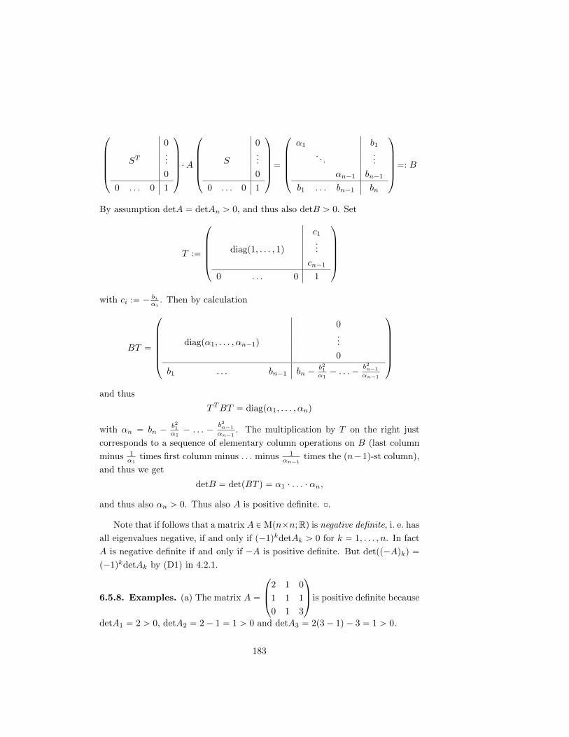
0

ST...

0

0 . . . 0 1

˛

‹

‹

‹

‹

‚

Ä

¨

˚

˚

˚

˚

˝

0

S...

0

0 . . . 0 1

˛

‹

‹

‹

‹

‚

“

¨

˚

˚

˚

˚

˝

α1 b1. . .

...

αn´1 bn´1

b1 . . . bn´1 bn

˛

‹

‹

‹

‹

‚

“: B

By assumption detA “ detAn ą 0, and thus also detB ą 0. Set

T :“

¨

˚

˚

˚

˚

˝

c1

diagp1, . . . , 1q...

cn´1

0 . . . 0 1

˛

‹

‹

‹

‹

‚

with ci :“ ´ biαi

. Then by calculation

BT “

¨

˚

˚

˚

˚

˚

˝

0

diagpα1, . . . , αn´1q...

0

b1 . . . bn´1 bn ´b21α1´ . . .´

b2n´1

αn´1

˛

‹

‹

‹

‹

‹

‚

and thus

TTBT “ diagpα1, . . . , αnq

with αn “ bn ´b21α1´ . . . ´

b2n´1

αn´1. The multiplication by T on the right just

corresponds to a sequence of elementary column operations on B (last column

minus 1α1

times first column minus . . . minus 1αn´1

times the pn´1q-st column),

and thus we get

detB “ detpBT q “ α1 ¨ . . . ¨ αn,

and thus also αn ą 0. Thus also A is positive definite. ˝.

Note that if follows that a matrix A P Mpnˆn;Rq is negative definite, i. e. has

all eigenvalues negative, if and only if p´1qkdetAk ą 0 for k “ 1, . . . , n. In fact

A is negative definite if and only if Á is positive definite. But detppÁqkq “

p´1qkdetAk by (D1) in 4.2.1.

6.5.8. Examples. (a) The matrix A “

¨

˚

˝

2 1 0

1 1 1

0 1 3

˛

‹

‚

is positive definite because

detA1 “ 2 ą 0, detA2 “ 2´ 1 “ 1 ą 0 and detA3 “ 2p3´ 1q ´ 3 “ 1 ą 0.

183

(b) The matrix A “

¨

˚

˝

´1 1 0

1 ´2 1

0 1 ´3

˛

‹

‚

is negative definite because detA1 “ ´1 ă

0, detA2 “ 2´ 1 ą 0 and detA3 “ ´1p6´ 1q ´ p´3q ´ 5` 3 “ ´2 ă 0.

The Hurwitz theorem is used to determine the definiteness of the Hesse

matrix for functions f : Rn Ñ R. For example if the Hesse matrix at a critical

point is positive definite then f has a minimum at this point.

184

Chapter 7

Jordan canonical form

7.1 The canonical form theorem

A matrix J P Mpr ˆ r;Kq is called a Jordan matrix for the eigenvalue λ P K if

J “

¨

˚

˚

˚

˚

˚

˚

˚

˝

λ 1 0 . . . 0

0 λ 1 0 . . . 0...

. . .. . . 0

... λ 1

0 . . . 0 λ

˛

‹

‹

‹

‹

‹

‹

‹

‚

For r “ 1, 2, 3 the Jordan matrices are explicitly:

r “ 1 : pλq; r “ 2 :

˜

λ 1

0 λ

¸

; r “ 3 :

¨

˚

˝

λ 1 0

0 λ 1

0 0 λ

˛

‹

‚

7.1.1. Theorem on the Jordan canonical form. Let dimKV ă 8 and

F P LKpV q. If the characteristic polynomial PF completely factorizes into linear

factors then there exists a basis B of V such that

MBpF q “

¨

˚

˚

˚

˚

˝

J1

J2 0

0. . .

J`

˛

‹

‹

‹

‹

‚

185

where J1, . . . , J` are Jordan matrices. We say that the matrix MBpF q has Jordan

normal form or Jordan canonical form. Note that the number ` of Jordan

matrices can in general be larger than the number of eigenvalues of F . For

example˜

2 0

0 2

¸

has only eigenvalue 2 but ` “ 2.

Before we discuss the proof we note the following.

7.1.2. Corollary. Each endomorphism of a complex vector space can be rep-

resented by a matrix in Jordan normal form. ˝

We will give now a proof of the Jordan normal form using only elementary

tools of linear algebra. The proof can be simplified considerably if results about

divisibility in polynomial rings are used.

Recall that for λ P K eigenvalue of the endomorphism F the eigenspace is

defined by

EigpF ;λq “ tv P V : F pvq “ λvu “ kerpF ´ λ ¨ idV q Ă V.

A necessary and sufficient condition for diagonalizability of F is that V is the

direct sum of the eigenspaces of F , see 5.3.3. The basic idea is to consider in

the general case the powers of F ´λ ¨ idV and to define a generalized eigenspace

(Hau does abbreviate the German word Haupt, which means Main.)

HaupF ;λq :“8ď

s“1

kerpF ´ λidV qs Ă V

The first step towards the Jordan normal form is:

7.1.3. Theorem about the decomposition into generalized eigenspaces.

Let F P LKpV q such that the characteristic polynomial PF factorizes completely

into linear factors. If

PF “ ˘pt´ λ1qr1 ¨ . . . ¨ pt´ λkq

rk

are pairwise distinct λ1, . . . , λk P K then we define for i “ 1, . . . , k

Wi :“ HaupF ;λiq.

Then there is a direct sum decomposition

V “W1 ‘ . . .‘Wk

186

and for i “ 1, . . . , k the following holds:

a) Wi “ kerpF ´ λi ¨ idV qri ,

b) dimWi “ ri,

c) F pWiq ĂWi,

d) PF |Wi“ ˘pt´ λiq

ri ,

e) pF |Wi ´ λi ¨ idWiqri “ 0.

For the proof we need the following

7.1.4. Lemma. Suppose the assumptions in 7.1.3. and let λ P K be an

eigenvalue of F of multiplicity r. Then there is a direct sum decomposition

V “W ‘ U

with the following properties:

a) W “ kerpF ´ λ ¨ idV qr “ HaupF ;λq,

b) dimW “ r,

c) F pW q ĂW and F pUq Ă U ,

d) PF |W “ ˘pt´ λqr,

e) pF |W ´ λ ¨ idW qr “ 0.

From 7.1.4 we deduce the decomposition of V into generalized eigenspaces

by induction over the number k of distinct eigenvalues.

For k “ 0 there is nothing to be shown because V “ t0u in this case. If

k ě 1 we get from 7.1.4 a direct sum decomposition

V “W1 ‘ U,

such that for i “ 1 the claims a) to e) hold. A basis of W1 and a basis of U

complete to a basis of V . If we calculate the characteristic polynomial using

the matrix representative with respect to this basis it follows from F pW1q ĂW1

and F pUq Ă U using 4.3.1

PF “ PF |W1¨ PF |U .

187

Thus

PF |U “ ˘pt´ λ2qr2 ¨ . . . ¨ pt´ λkq

rk .

By induction hypothesis there is a decomposition

U “W 12 ‘ . . .‘W

1k, with

W 1i “ HaupF |U ;λiq Ă U for i “ 2, . . . , k.

Obviously W 1i Ă Wi. By induction hypothesis dimW 1

i “ ri and thus by 7.1.4

applied to λ “ λi it follows dimWi “ ri. Thus W 1i “Wi and

V “W1 ‘ . . .‘Wk.

The properties a)-e) hold for i “ 1 by 7.1.4 and for i “ 2, . . . , k by induction

hypothesis.

Proof of 7.1.4: We will use 5.4.4, i. e. the fact that F can be triangulated. Let

v1, . . . , vn be a basis of V such that F is represented by the matrix

A “

˜

λIr `N C

0 D

¸

Here D is an upper triangular pn´rqˆpn´rq-matrix, and for the prˆrq-matrix

N “ pnijqij we have nij “ 0 for i ě j. Then G :“ F ´ λ ¨ idV is described by

B “

˜

N C

0 D1

¸

where D1 “ D ´ λ ¨ In´r. In the diagonal of D appear the eigenvalues of F

distinct from λ, and thus the diagonal components of D1 are not zero, and it

follows

rankD1 “ n´ r.

It is now easy to compute that for s ě 1:

Bs “

˜

Ns Cs

0 Ds1

¸

.

Now consider the chain

kerG Ă kerG2 Ă . . . Ă kerGr Ă . . . Ă kerGs,

where r ď s. Because of the special form of the matrix N it follows by simple

computation that Nr “ 0. So for all s ě r also Ns “ 0 and

dimpimGsq “ rankBs “ rankDs1 “ rankpD1q “ n´ r.

188

It can be seen from the matrix Bs that v1, . . . , vr P kerGs, and thus by the

dimension formula 2.2.4

kerGs “ spanpv1, . . . , vrq.

In particular

kerGr “ kerGr`1 “ . . . “ kerGs

and

W “ HaupF ;λq “8ď

s“1

kerGs “ kerGr.

We set

U :“ imGr.

To show that V “ W ‘ U it suffices because of n “ dimW ` dimU to check

V “W ` U , compare 1.6. But this follows immediately from

rank

˜

Ir Cr

0 Dr1

¸

“ n,

because the first r columns of this matrix span the kernel, the last n ´ r span

the image of Gr with respect to the basis pv1, . . . , vnq. Obviously GpkerGr`1q Ă

kerGr (this is just restating GrpGvq “ Gr`1v, so v P kerGr`1 ùñ GrpGvq “

0 ùñ Gv P kerGr.) As seen above

kerGr`1 “ kerGr, thus GpW q ĂW and so F pW q ĂW.

Similarly GpimGrq “ imGr`1 Ă imGr, and thus

GpUq Ă U, and thus F pUq Ă U.

Thus a)-c) have been proven. To show d) and e) it suffices to note that F |W is

described with respect to the basis pv1, . . . , vrq of W by the matrix λ ¨ Ir`N . ˝

Using the fundamental theorem of algebra the decomposition into gener-

alized eigenspaces gives the following important result for complex matrices,

which is useful for the solution of systems of differential equations.

7.1.5. Corollary. For each A P Mpn ˆ n;Cq there exists S P GLpn;Cq such

189

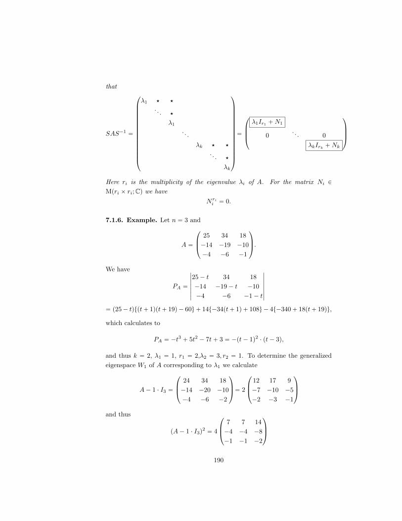
that

SAS´1 “

¨

˚

˚

˚

˚

˚

˚

˚

˚

˚

˚

˚

˚

˚

˝

λ1 ‹ ‹

. . . ‹

λ1

. . .

λk ‹ ‹

. . . ‹

λk

˛

‹

‹

‹

‹

‹

‹

‹

‹

‹

‹

‹

‹

‹

‚

“

¨

˚

˚

˝

λ1Ir1 `N1

0. . . 0

λkIrk `Nk

˛

‹

‹

‚

Here ri is the multiplicity of the eigenvalue λi of A. For the matrix Ni P

Mpri ˆ ri;Cq we have

Nrii “ 0.

7.1.6. Example. Let n “ 3 and

A “

¨

˚

˝

25 34 18

´14 ´19 ´10

´4 ´6 ´1

˛

‹

‚

.

We have

PA “

∣∣∣∣∣∣∣25´ t 34 18

´14 ´19´ t ´10

´4 ´6 ´1´ t

∣∣∣∣∣∣∣“ p25´ tqtpt` 1qpt` 19q ´ 60u ` 14t´34pt` 1q ` 108u ´ 4t´340` 18pt` 19qu,

which calculates to

PA “ ´t3 ` 5t2 ´ 7t` 3 “ ´pt´ 1q2 ¨ pt´ 3q,

and thus k “ 2, λ1 “ 1, r1 “ 2,λ2 “ 3, r2 “ 1. To determine the generalized

eigenspace W1 of A corresponding to λ1 we calculate

A´ 1 ¨ I3 “

¨

˚

˝

24 34 18

´14 ´20 ´10

´4 ´6 ´2

˛

‹

‚

“ 2

¨

˚

˝

12 17 9

´7 ´10 ´5

´2 ´3 ´1

˛

‹

‚

and thus

pA´ 1 ¨ I3q2 “ 4

¨

˚

˝

7 7 14

´4 ´4 ´8

´1 ´1 ´2

˛

‹

‚

190

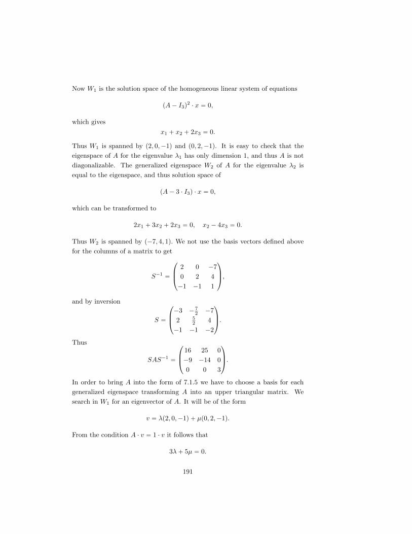
Now W1 is the solution space of the homogeneous linear system of equations

pA´ I3q2 ¨ x “ 0,

which gives

x1 ` x2 ` 2x3 “ 0.

Thus W1 is spanned by p2, 0,´1q and p0, 2,´1q. It is easy to check that the

eigenspace of A for the eigenvalue λ1 has only dimension 1, and thus A is not

diagonalizable. The generalized eigenspace W2 of A for the eigenvalue λ2 is

equal to the eigenspace, and thus solution space of

pA´ 3 ¨ I3q ¨ x “ 0,

which can be transformed to

2x1 ` 3x2 ` 2x3 “ 0, x2 ´ 4x3 “ 0.

Thus W2 is spanned by p´7, 4, 1q. We not use the basis vectors defined above

for the columns of a matrix to get

S´1 “

¨

˚

˝

2 0 ´7

0 2 4

´1 ´1 1

˛

‹

‚

,

and by inversion

S “

¨

˚

˝

´3 ´ 72 ´7

2 52 4

´1 ´1 ´2

˛

‹

‚

.

Thus

SAS´1 “

¨

˚

˝

16 25 0

´9 ´14 0

0 0 3

˛

‹

‚

.

In order to bring A into the form of 7.1.5 we have to choose a basis for each

generalized eigenspace transforming A into an upper triangular matrix. We

search in W1 for an eigenvector of A. It will be of the form

v “ λp2, 0,´1q ` µp0, 2,´1q.

From the condition A ¨ v “ 1 ¨ v it follows that

3λ` 5µ “ 0.

191

Thus we can choose v “ p5,´3,´1q. Together with 2, 0,´1q this defines a basis

of W1. We get new transformation matrices

T´1 “

¨

˚

˝

5 2 ´7

´3 0 4

´1 ´1 1

˛

‹

‚

, and T “1

3

¨

˚

˝

´4 ´5 ´8

1 2 ´1

´3 ´3 ´6

˛

‹

‚

,

and so

TAT´1 “

¨

˚

˝

1 6 0

0 1 0

0 0 3

˛

‹

‚

.

We can use the transformation above to find the general solution of the

system of differential equations:

y1ptq “ Ayptq, yp0q “ c

In fact we will solve the matrix differential equation

Y 1ptq “ AY ptq

by the transformation Y ptq “ T´1Xptq. Then

X 1ptq “ TAT´1Xptq

For TAT´1 in normal form as above it follows that

Xptq “

¨

˚

˝

et 6tet 0

0 et 0

0 0 e3t

˛

‹

‚

satisfies the above matrix equation because we can calculate:¨

˚

˝

1 6 0

0 1 0

0 0 3

˛

‹

‚

¨

˚

˝

et 6tet 0

0 et 0

0 0 e3t

˛

‹

‚

“

¨

˚

˝

et 6tet ` 6et 0

0 et 0

0 0 3e3t

˛

‹

‚

“

¨

˚

˝

et 6tet 0

0 et 0

0 0 e3t

˛

‹

‚

1

Now consider yptq :“ T´1XptqTc then

y1ptq “ T´1X 1ptqTc “ T´1pTAT´1XptqqTc “ Ayptq, yp0q “ T´1I3Tc “ c,

which is the general solution of the system of differential equations. We can

also say that Y ptq :“ T´1XptqT solves the matrix equation Y 1ptq “ AY ptq and

Y p0q “ I3 and thus is a fundamental solutions matrix. So for the above

Y ptq “1

3

¨

˚

˝

5 2 ´7

´3 0 4

´1 ´1 1

˛

‹

‚

¨

˚

˝

et 6tet 0

0 et 0

0 0 e3t

˛

‹

‚

¨

˚

˝

´4 ´5 ´8

1 2 ´1

´3 ´3 6

˛

‹

‚

,

192

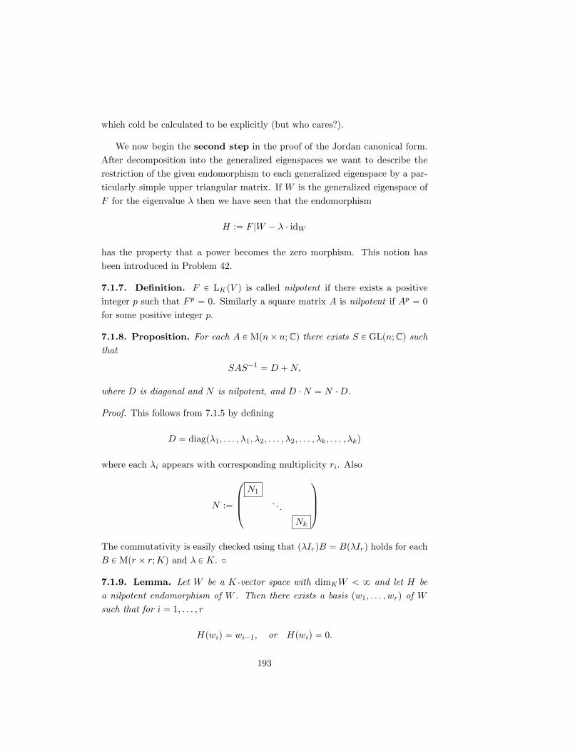
which cold be calculated to be explicitly (but who cares?).

We now begin the second step in the proof of the Jordan canonical form.

After decomposition into the generalized eigenspaces we want to describe the

restriction of the given endomorphism to each generalized eigenspace by a par-

ticularly simple upper triangular matrix. If W is the generalized eigenspace of

F for the eigenvalue λ then we have seen that the endomorphism

H :“ F |W ´ λ ¨ idW

has the property that a power becomes the zero morphism. This notion has

been introduced in Problem 42.

7.1.7. Definition. F P LKpV q is called nilpotent if there exists a positive

integer p such that F p “ 0. Similarly a square matrix A is nilpotent if Ap “ 0

for some positive integer p.

7.1.8. Proposition. For each A P Mpnˆ n;Cq there exists S P GLpn;Cq such

that

SAS´1 “ D `N,

where D is diagonal and N is nilpotent, and D ¨N “ N ¨D.

Proof. This follows from 7.1.5 by defining

D “ diagpλ1, . . . , λ1, λ2, . . . , λ2, . . . , λk, . . . , λkq

where each λi appears with corresponding multiplicity ri. Also

N :“

¨

˚

˚

˝

N1

. . .

Nk

˛

‹

‹

‚

The commutativity is easily checked using that pλIrqB “ BpλIrq holds for each

B P Mpr ˆ r;Kq and λ P K. ˝

7.1.9. Lemma. Let W be a K-vector space with dimKW ă 8 and let H be

a nilpotent endomorphism of W . Then there exists a basis pw1, . . . , wrq of W

such that for i “ 1, . . . , r

Hpwiq “ wi´1, or Hpwiq “ 0.

193

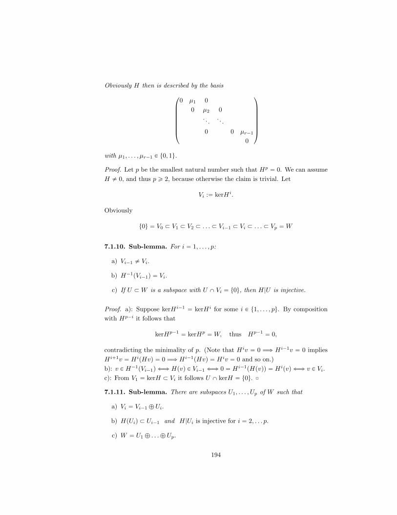
Obviously H then is described by the basis

¨

˚

˚

˚

˚

˚

˚

˝

0 µ1 0

0 µ2 0. . .

. . .

0 0 µr´1

0

˛

‹

‹

‹

‹

‹

‹

‚

with µ1, . . . , µr´1 P t0, 1u.

Proof. Let p be the smallest natural number such that Hp “ 0. We can assume

H ‰ 0, and thus p ě 2, because otherwise the claim is trivial. Let

Vi :“ kerHi.

Obviously

t0u “ V0 Ă V1 Ă V2 Ă . . . Ă Vi´1 Ă Vi Ă . . . Ă Vp “W

7.1.10. Sub-lemma. For i “ 1, . . . , p:

a) Vi´1 ‰ Vi.

b) H´1pVi´1q “ Vi.

c) If U ĂW is a subspace with U X Vi “ t0u, then H|U is injective.

Proof. a): Suppose kerHi´1 “ kerHi for some i P t1, . . . , pu. By composition

with Hp´i it follows that

kerHp´1 “ kerHp “W, thus Hp´1 “ 0,

contradicting the minimality of p. (Note that Hiv “ 0 ùñ Hi´1v “ 0 implies

Hi`1v “ HipHvq “ 0 ùñ Hi´1pHvq “ Hiv “ 0 and so on.)

b): v P H´1pVi´1q ðñ Hpvq P Vi´1 ðñ 0 “ Hi´1pHpvqq “ Hipvq ðñ v P Vi.

c): From V1 “ kerH Ă Vi it follows U X kerH “ t0u. ˝

7.1.11. Sub-lemma. There are subspaces U1, . . . , Up of W such that

a) Vi “ Vi´1 ‘ Ui.

b) HpUiq Ă Ui´1 and H|Ui is injective for i “ 2, . . . p.

c) W “ U1 ‘ . . .‘ Up.

194

Proof. This follows from 7.1.10. A direct summand Up of Vp´1 in Vp is chosen

arbitrarily; thus

W “ Vp “ Vp´1 ‘ Up.

From H´1pVp´2q “ Vp´1 it follows HpUpqXVp´2 “ t0u. (In fact if v P HpUpqX

Vp´2 then v “ Hpuq for some u P Up. But v P Vp´2 and H´1Vp´2 “ Vp´1,

thus v P Vp´1. It follows that u P Up X Vp´1 “ t0u.) Thus there is a subspace

Up´1 Ă Vp´1 such that

Vp´1 “ Vp´2 ‘ Up´1 and HpUpq Ă Up´1.

This procedure can be iterated. If for i P t2, . . . , pu the decomposition

Vi “ Vi´1 ‘ Ui

is already given then analogous to the above for the case i “ p

Vi´1 “ Vi´2 ‘ Ui´1, where HpUiq Ă Ui´1.

From Ui X Vi´1 “ t0u follows b). Finally claim c) follows from

W “ Vp “ Vp´1 ‘ Up “ Vp´2 ‘ Up´1 ‘ Up “ . . . “ V0 ‘ U1 ‘ . . .‘ Up

because V0 “ t0u. ˝

We return to the proof of 7.1.9. Now we have the tools available to construct

a basis with the required properties. There are numbers li P N for i “ 1, . . . p

and corresponding basis vectors:

Basis of:

Up : uppq1 , . . . , u

ppqlp

Up´1 : Hpuppq1 q, . . . ,Hpu

ppqlpq, u

pp´1q1 , . . . , u

pp´1qlp´1

......

...

U1 : Hpp´1qpuppq1 q, . . . ,Hpp´1qpu

ppqlpq, Hpp´2qpu

pp´1q1 q, . . .

, Hpp´2qpupp´1qlp´1

q, . . . , up1q1 , . . . , u

p1ql1

All the vectors in the scheme above form a basis of W . Because of

U1 “ V0 ‘ U1 “ V1 “ kerH1 “ kerH

the endomorphism H maps the vectors in U1 to 0. Note that

dimUp “ lp,dimUp´1 “ lp ` lp´1, . . . ,dimU1 “ lp ` . . .` l1,

195

and thus

r “ plp ` pp´ 1qlp´1 ` . . .` 2l2 ` l1 “ r.

We can reorder the basis vectors column-wise from the bottom to the top:

w1 :“ Hpp´1qpuppq1 q, . . . , wp :“ u

ppq1 ,

wp`1 :“ Hpp´1qpuppq2 q, . . . , w2p :“ u

ppq2 ,

...

wplp`1 :“ Hpp´2qpupp´1q1 q, . . . , wplp`p´1 :“ u

pp´1q1 ,

...

wr´l1`1 :“ up1q1 ,

...

wr :“ up1ql1.

This proves 7.1.9 and thus also the theorem on the Jordan canonical form 7.1.1.

˝

Note that, from the above basis constructed for a specific eigenvalue λ of

A P LKpV q, we get lp Jordan blocks of size p, lp´1 Jordan blocks of size p´ 1,

and so on, until finally l1 Jordan blocks of size 1.

7.1.12. Example. We want to transform the matrix

A “

¨

˚

˝

3 4 3

´1 0 ´1

1 2 3

˛

‹

‚

into Jordan canonical form. In 5.4.6 we did already triangulate this matrix.

Using

S “

¨

˚

˝

1 0 0

1 1 0

0 1 1

˛

‹

‚

, and S´1 “

¨

˚

˝

1 0 0

´1 1 0

1 ´1 1

˛

‹

‚

we had

SAS´1 “

¨

˚

˝

2 1 3

0 2 2

0 0 2

˛

‹

‚

“: rA.

196

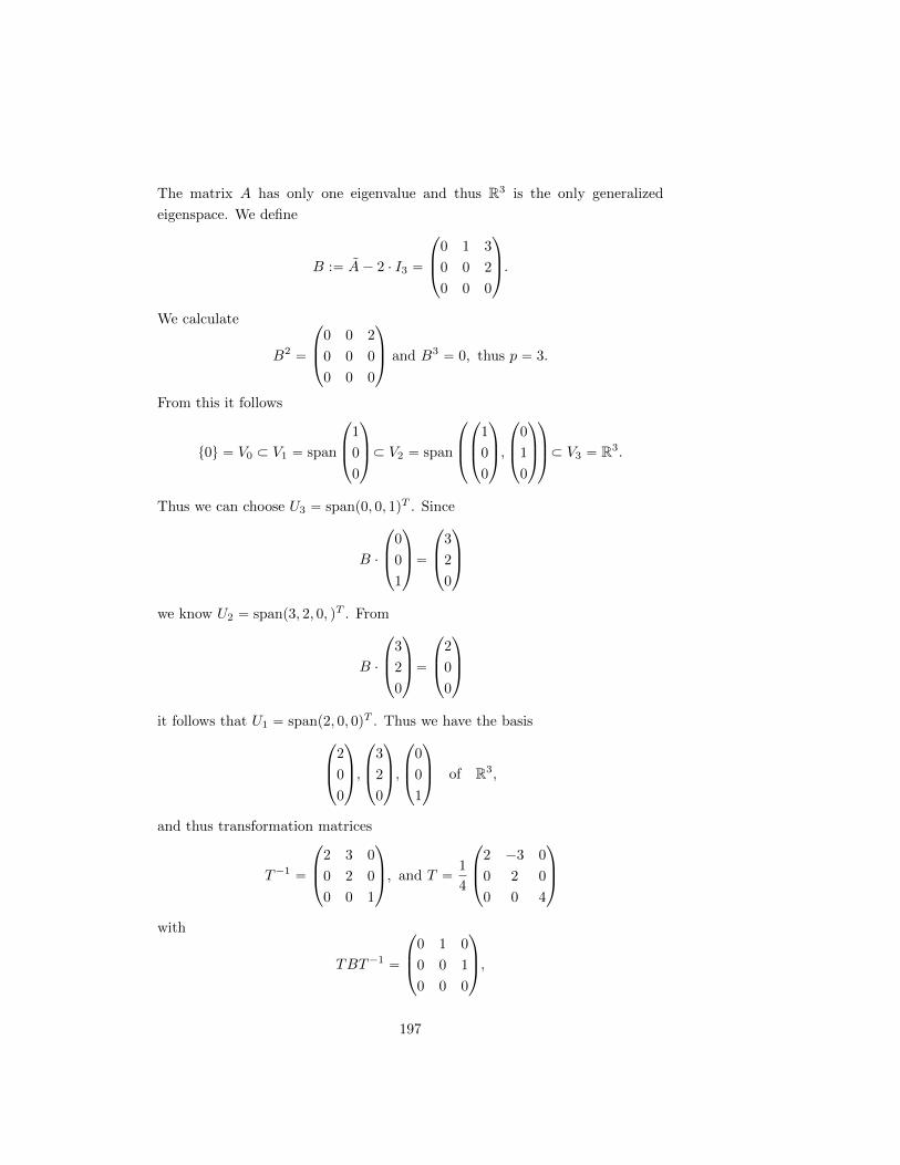
The matrix A has only one eigenvalue and thus R3 is the only generalized

eigenspace. We define

B :“ A´ 2 ¨ I3 “

¨

˚

˝

0 1 3

0 0 2

0 0 0

˛

‹

‚

.

We calculate

B2 “

¨

˚

˝

0 0 2

0 0 0

0 0 0

˛

‹

‚

and B3 “ 0, thus p “ 3.

From this it follows

t0u “ V0 Ă V1 “ span

¨

˚

˝

1

0

0

˛

‹

‚

Ă V2 “ span

¨

˚

˝

¨

˚

˝

1

0

0

˛

‹

‚

,

¨

˚

˝

0

1

0

˛

‹

‚

˛

‹

‚

Ă V3 “ R3.

Thus we can choose U3 “ spanp0, 0, 1qT . Since

B ¨

¨

˚

˝

0

0

1

˛

‹

‚

“

¨

˚

˝

3

2

0

˛

‹

‚

we know U2 “ spanp3, 2, 0, qT . From

B ¨

¨

˚

˝

3

2

0

˛

‹

‚

“

¨

˚

˝

2

0

0

˛

‹

‚

it follows that U1 “ spanp2, 0, 0qT . Thus we have the basis

¨

˚

˝

2

0

0

˛

‹

‚

,

¨

˚

˝

3

2

0

˛

‹

‚

,

¨

˚

˝

0

0

1

˛

‹

‚

of R3,

and thus transformation matrices

T´1 “

¨

˚

˝

2 3 0

0 2 0

0 0 1

˛

‹

‚

, and T “1

4

¨

˚

˝

2 ´3 0

0 2 0

0 0 4

˛

‹

‚

with

TBT´1 “

¨

˚

˝

0 1 0

0 0 1

0 0 0

˛

‹

‚

,

197

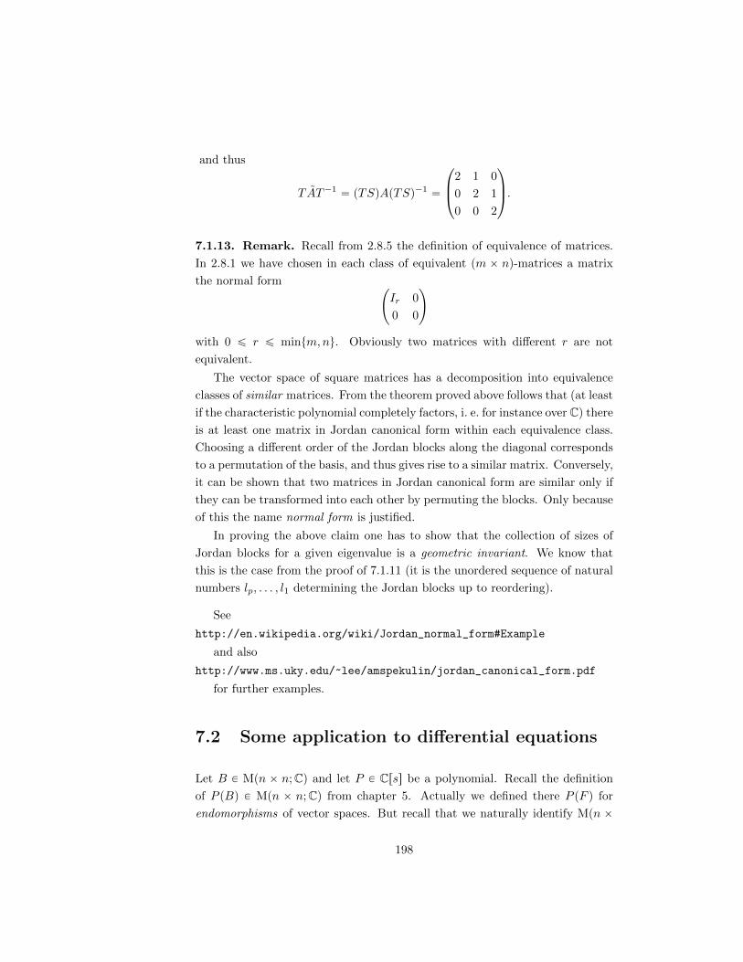
and thus

TAT´1 “ pTSqApTSq´1 “

¨

˚

˝

2 1 0

0 2 1

0 0 2

˛

‹

‚

.

7.1.13. Remark. Recall from 2.8.5 the definition of equivalence of matrices.

In 2.8.1 we have chosen in each class of equivalent pm ˆ nq-matrices a matrix

the normal form˜

Ir 0

0 0

¸

with 0 ď r ď mintm,nu. Obviously two matrices with different r are not

equivalent.

The vector space of square matrices has a decomposition into equivalence

classes of similar matrices. From the theorem proved above follows that (at least

if the characteristic polynomial completely factors, i. e. for instance over C) there

is at least one matrix in Jordan canonical form within each equivalence class.

Choosing a different order of the Jordan blocks along the diagonal corresponds

to a permutation of the basis, and thus gives rise to a similar matrix. Conversely,

it can be shown that two matrices in Jordan canonical form are similar only if

they can be transformed into each other by permuting the blocks. Only because

of this the name normal form is justified.

In proving the above claim one has to show that the collection of sizes of

Jordan blocks for a given eigenvalue is a geometric invariant. We know that

this is the case from the proof of 7.1.11 (it is the unordered sequence of natural

numbers lp, . . . , l1 determining the Jordan blocks up to reordering).

See

http://en.wikipedia.org/wiki/Jordan_normal_form#Example

and also

http://www.ms.uky.edu/~lee/amspekulin/jordan_canonical_form.pdf

for further examples.

7.2 Some application to differential equations

Let B P Mpn ˆ n;Cq and let P P Crss be a polynomial. Recall the definition

of P pBq P Mpn ˆ n;Cq from chapter 5. Actually we defined there P pF q for

endomorphisms of vector spaces. But recall that we naturally identify Mpn ˆ

198

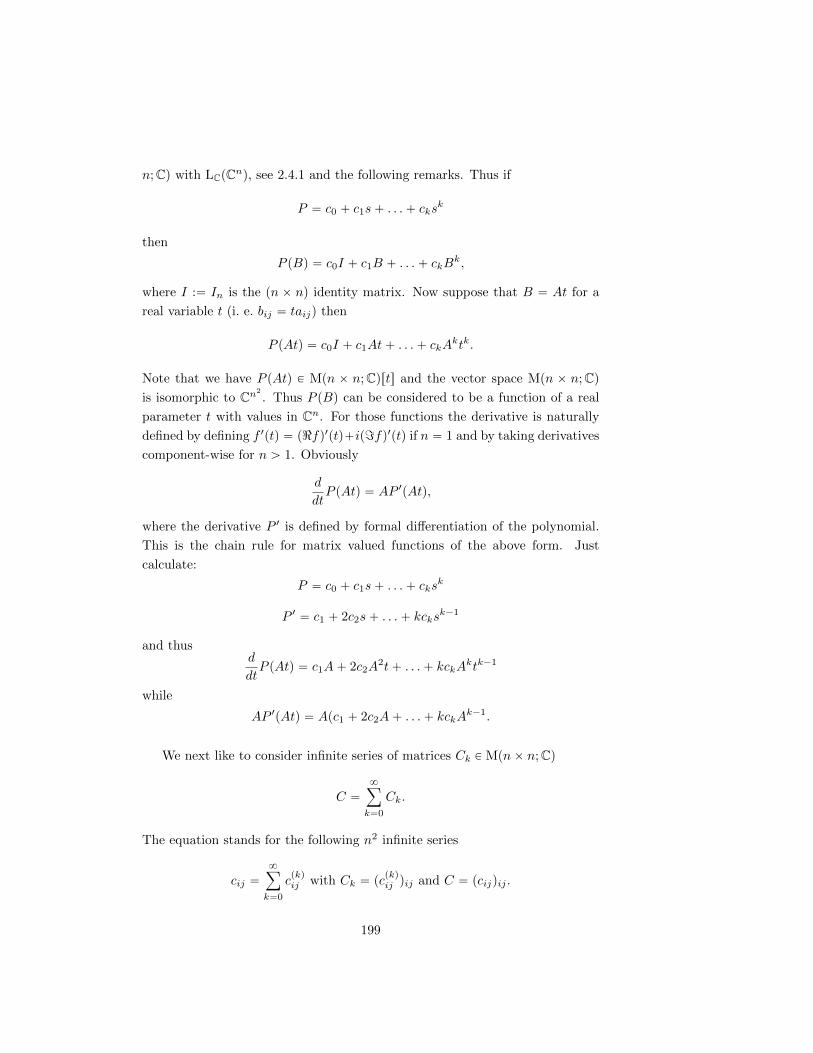
http://en.wikipedia.org/wiki/Jordan_normal_form#Example

http://www.ms.uky.edu/~lee/amspekulin/jordan_canonical_form.pdf

n;Cq with LCpCnq, see 2.4.1 and the following remarks. Thus if

P “ c0 ` c1s` . . .` cksk

then

P pBq “ c0I ` c1B ` . . .` ckBk,

where I :“ In is the pn ˆ nq identity matrix. Now suppose that B “ At for a

real variable t (i. e. bij “ taij) then

P pAtq “ c0I ` c1At` . . .` ckAktk.

Note that we have P pAtq P Mpn ˆ n;Cqrts and the vector space Mpn ˆ n;Cqis isomorphic to Cn2

. Thus P pBq can be considered to be a function of a real

parameter t with values in Cn. For those functions the derivative is naturally

defined by defining f 1ptq “ p<fq1ptq`ip=fq1ptq if n “ 1 and by taking derivatives

component-wise for n ą 1. Obviously

d

dtP pAtq “ AP 1pAtq,

where the derivative P 1 is defined by formal differentiation of the polynomial.

This is the chain rule for matrix valued functions of the above form. Just

calculate:

P “ c0 ` c1s` . . .` cksk

P 1 “ c1 ` 2c2s` . . .` kcksk´1

and thusd

dtP pAtq “ c1A` 2c2A

2t` . . .` kckAktk´1

while

AP 1pAtq “ Apc1 ` 2c2A` . . .` kckAk´1.

We next like to consider infinite series of matrices Ck P Mpnˆ n;Cq

C “8ÿ

k“0

Ck.

The equation stands for the following n2 infinite series

cij “8ÿ

k“0

cpkqij with Ck “ pc

pkqij qij and C “ pcijqij .

199

The matrix series is convergent respectively absolutely convergent if each of the

n2 scalar series has this property. In particular each power series

fpsq “8ÿ

k“0

cksk p|s| ă rq

with radius of convergence r gives rise to a matrix function

fpBq “8ÿ

k“0

ckBk pabsolutely convergent for ||B|| ă rq,

where ||B|| :“b

ř

i,j |bij |2 is the usual Euclidean norm on Cn2

derived from the

inner product. In fact, if ||B|| “: s ă r then

||B2|| ď ||B||2 “ s2, . . . , ||Bk|| ď sk.

Here we have used that ||AB|| ď ||A|| ¨ ||B||, which follows easily using the

triangle inequality in the real numbers:

||AB|| “ÿ

i,j

ˇ

ˇ

ˇ

ˇ

ˇ

ÿ

k

aikbkj

ˇ

ˇ

ˇ

ˇ

ˇ

ďÿ

i,j

ÿ

k

|aikbkj | ďÿ

i,j,k,l

|aikblj | “ ||A|| ¨ ||B||.

Thus the above series converges by the comparison test. In particular

fpAT q “ c0I ` c1At` c2A2t2 ` . . .

is absolutely convergent for

|t| ăr

||A||“: t0

and uniformly convergent (i. e. each of the n2 scalar series is uniformly con-

vergent) on each compact subinterval of p´t0, t0q Ă R). Since the formally

differentiated series is uniformly convergent again we can differentiate fpAtq

term by term. Thus, just as in the case of polynomials we have

d

dtfpAtq “ Af 1pAtq.

7.2.1. Example. The exponential function

eB “ I `B `B2

2`B3

3!` . . .

exists for all matrices B and

peAtq1 “ AeAt.

200

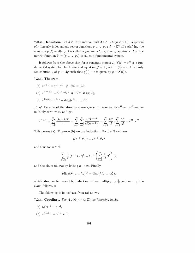
7.2.2. Definition. Let J Ă R an interval and A : J Ñ Mpnˆ n;Cq. A system

of n linearly independent vector functions y1, . . . , yn : J Ñ Cn all satisfying the

equation y1ptq “ Aptqyptq is called a fundamental system of solutions. Also the

matrix function Y “ py1, . . . , ynq is called a fundamental system.

It follows from the above that for a constant matrix A, Y ptq “ eAt is a fun-

damental system for the differential equation y1 “ Ay with Y p0q “ I. Obviously

the solution y of y1 “ Ay such that yp0q “ c is given by y “ Xptqc.

7.2.3. Theorem.

(a) eB`C “ eB ¨ eC if BC “ CB,

(b) eC´1BC “ C´1eBC if C P GLpn;Cq,

(c) ediagpλ1,...,λnq “ diagpeλ1 , . . . , eλnq

Proof. Because of the absoulte convergence of the series for eB and eC we can

multiply term-wise, and get

eB`C “8ÿ

n“0

pB ` Cqn

n!“

8ÿ

n“0

nÿ

k“0

BkCn´k

k!pn´ kq!“

8ÿ

p“0

Bp

p!¨

8ÿ

q“0

Cq

q!“ eB ¨ eC

This proves (a). To prove (b) we use induction. For k P N we have

pC´1BCqk “ C´1BkC

and thus for n P N:

nÿ

k“0

1

k!pC´1BCqk “ C´1

˜

nÿ

k“0

1

k!Bk

¸

C,

and the claim follows by letting nÑ8. Finally

pdiagpλ1, . . . , λnqqk “ diagpλk1 , . . . , λ

knq,

which also can be proved by induction. If we multiply by 1k! and sum up the

claim follows. ˝

The following is immediate from (a) above.

7.2.4. Corollary. For A P Mpnˆ n;Cq the following holds:

(a) peAq´1 “ e´A,

(b) eAps`tq “ aAs ¨ eAt,

201

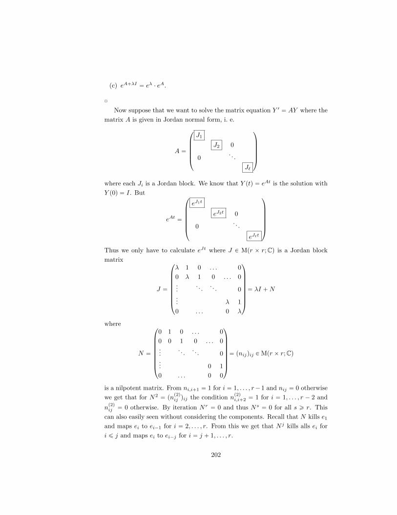
(c) eA`λI “ eλ ¨ eA.

˝

Now suppose that we want to solve the matrix equation Y 1 “ AY where the

matrix A is given in Jordan normal form, i. e.

A “

¨

˚

˚

˚

˚

˝

J1

J2 0

0. . .

J`

˛

‹

‹

‹

‹

‚

where each Ji is a Jordan block. We know that Y ptq “ eAt is the solution with

Y p0q “ I. But

eAt “

¨

˚

˚

˚

˚

˚

˝

eJ1t

eJ2t 0

0. . .

eJ`t

˛

‹

‹

‹

‹

‹

‚

Thus we only have to calculate eJt where J P Mpr ˆ r;Cq is a Jordan block

matrix

J “

¨

˚

˚

˚

˚

˚

˚

˚

˝

λ 1 0 . . . 0

0 λ 1 0 . . . 0...

. . .. . . 0

... λ 1

0 . . . 0 λ

˛

‹

‹

‹

‹

‹

‹

‹

‚

“ λI `N

where

N “

¨

˚

˚

˚

˚

˚

˚

˚

˝

0 1 0 . . . 0

0 0 1 0 . . . 0...

. . .. . . 0

... 0 1

0 . . . 0 0

˛

‹

‹

‹

‹

‹

‹

‹

‚

“ pnijqij P Mpr ˆ r;Cq

is a nilpotent matrix. From ni,i`1 “ 1 for i “ 1, . . . , r´1 and nij “ 0 otherwise

we get that for N2 “ pnp2qij qij the condition n

p2qi,i`2 “ 1 for i “ 1, . . . , r ´ 2 and

np2qij “ 0 otherwise. By iteration Nr “ 0 and thus Ns “ 0 for all s ě r. This

can also easily seen without considering the components. Recall that N kills e1

and maps ei to ei´1 for i “ 2, . . . , r. From this we get that N j kills alls ei for

i ď j and maps ei to ei´j for i “ j ` 1, . . . , r.

202

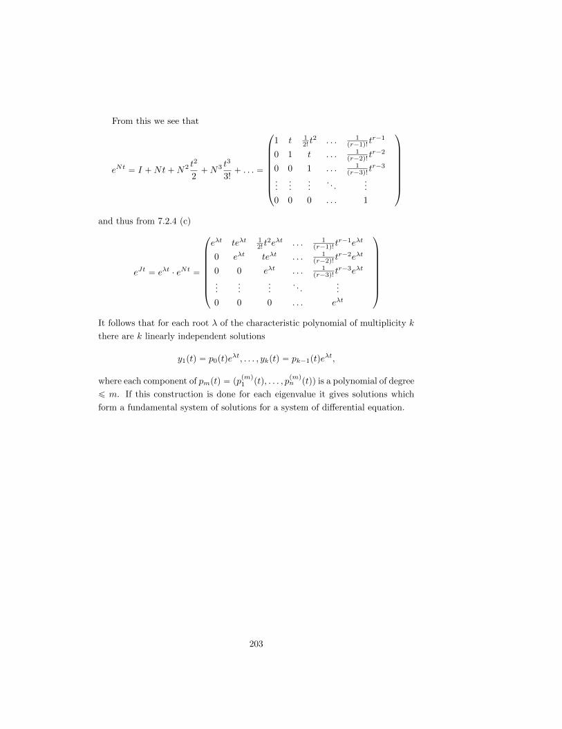
From this we see that

eNt “ I `Nt`N2 t2

2`N3 t

3

3!` . . . “

¨

˚

˚

˚

˚

˚

˚

˚

˝

1 t 12! t

2 . . . 1pr´1q! t

r´1

0 1 t . . . 1pr´2q! t

r´2

0 0 1 . . . 1pr´3q! t

r´3

......

.... . .

...

0 0 0 . . . 1

˛

‹

‹

‹

‹

‹

‹

‹

‚

and thus from 7.2.4 (c)

eJt “ eλt ¨ eNt “

¨

˚

˚

˚

˚

˚

˚

˚

˝

eλt teλt 12! t

2eλt . . . 1pr´1q! t

r´1eλt

0 eλt teλt . . . 1pr´2q! t

r´2eλt

0 0 eλt . . . 1pr´3q! t

r´3eλt

......

.... . .

...

0 0 0 . . . eλt

˛

‹

‹

‹

‹

‹

‹

‹

‚

It follows that for each root λ of the characteristic polynomial of multiplicity k

there are k linearly independent solutions

y1ptq “ p0ptqeλt, . . . , ykptq “ pk´1ptqe

λt,

where each component of pmptq “ pppmq1 ptq, . . . , p

pmqn ptqq is a polynomial of degree

ď m. If this construction is done for each eigenvalue it gives solutions which

form a fundamental system of solutions for a system of differential equation.

203

notes on linear algebra - department of mathematics...

Documents