notes on compressible flow
TRANSCRIPT
Notes on compressible flow
Stephen Childress
February 27, 2006
1 Mechanical energy
We recall the two conservation laws from the first semester:Conservation of mass:
∂ρ
∂t+ ∇ · (ρu) = 0, (1)
Conservation of momentum:
∂(ρui)∂t
+∂(ρuiuj)∂xj
= ρDui
Dt= Fi +
∂σij
∂xj,D
Dt=
∂
∂t+ u · ∇. (2)
Here σij are the components of the viscous stress tensor: 1
σij = −pδij + µ[ ∂ui
∂xj+∂uj
∂xi− 2
3δij∇ · u
]. (3)
We now want to use these results to compute the rate of change of totalkinetic energy within a fixed fluid volume V . We see that
d
dt
∫
V
12ρu2dV =
∫
V
[ρui
∂ui
∂t+
12∂ρ
∂tu2
]dV
=∫
V
([− ρuj
∂ui
xj+∂σij
∂xj+ Fi
]ui −
12∂ρuj
∂xju2
)dV
=∫
V
[uiFi + p∇ · u
]dV − Φ +
∫
S
[− 1
2ρuju
2 + uiσij
]njdS, (4)
where S is the boundary of V and Φ is the total viscous dissipation in V :
Φ =∫
φ
dV, φ = µ[12( ∂ui
∂xj+∂uj
∂xi
)2 − 23(∇ · u)2
]. (5)
1You will find that Landau and Lifshitz allow a deviation from the Stokes relation. Recallthat this relation makes the trace of the non-pressure part of the stress tensor (the deviatoricstress) zero. This deviation is accomplished by adding a term µ′δij∇ · u to the stress tensor,where µ′ is called the second viscosity. For simplicity, and sionce the exact form is not materialto the problems we shall study, we neglect this second viscosity in the present notes. Howeverfor applications to real gases it should be retained as the Stokes relation does not hold formany gases.
1
We note from (4) that the contributions in order come from the work done bybody forces, the work done by pressure in compression, viscous heating, flux ofkinetic energy through S, and work done by stresses on S. We refer to (4) asthe mechanical energy equation, since we have use only conservation of massand momentum.
To put this expression into a different form we now complete the fluid equa-tions by assuming a barotropic fluid, p = p(ρ). Then
∫
V
p∇ · udV =∫
S
pu · ndS −∫
V
u · ∇pdV. (6)
But ∫
V
u · ∇pdV =∫ρu · ∇
∫1ρp′(ρ)dρdV
=∫
S
ρ
∫1ρp′(ρ)dρu · ndS +
∫
V
∂ρ
∂t
∫1ρp′(ρ)dρdV. (7)
We now define g(ρ) by∫
1ρp′(ρ)dρ = g′(ρ), g(0) = 0. (8)
and define e byg = ρe. (9)
Noting that
d
dρ
(p− ρ
∫1ρp′(ρ)dρ
)= −
∫1ρp′(ρ)dρ = −g′ = −(ρe)′, (10)
we have thatp− ρ
∫1ρp′(ρ)dρ = −ρe. (11)
Thus ∫
V
u · ∇pdV = −∫
S
ρeu · ndS −∫
∂ρ
∂t(ρe)′dV. (12)
Using this in (4) we obtain
d
dt
∫
V
EdV +∫
S
Eu ·ndS = −Φ +∫
V
uiFidV +∫
S
uiσijnjdS, (13)
whereE = ρ
(e +
12u2
). (14)
Note that if µ = 0 and Fi = 0 then (13) reduces to a conservation law of theform
d
dt
∫
V
EdV +∫
S
(E + p)u ·ndS (15)
2
We note that E should have the meaning of energy, and we shall refer to e asthe internal energy of the fluid (per unit mass). Then (13) can be viewed asas expression of the first law of thermodynamics ∆E = ∆Q −W , where ∆Eis the change of energy of an isolated system (not flux of energy through theboundary), ∆Q is the heat added to the system, and W is the work done by thesystem.
The form of (13) can however be used as a model for formulating a moregeneral energy equation, and we shall do this after first reviewing some of thebasic concepts of reversible thermodynamics.
2 Elements of classical thermodynamics
Thermodynamics deals with transformations of energy within an isolated sys-tem. These transformations are determined by thermodynamic variables. Thesecome in two types: Extensive variables are proportional to the amount of ma-terial involved. Examples are internal energy, entropy, heat. Intensive variablesare not proportional to quantity. Examples are pressure, density, temperature.
We have just introduced to new scalar field, the absolute temperatureT , andthe specific entropy s. We shall also make use of specific volume v, defined byv = 1/ρ.
We now discuss the thermodynamics of gases. In general we shall assumethe existence of an equation of state of the gas, connecting p, ρ, T . An importantexample is the equation of state of an ideal or perfect gas, defined by
pv = RT. (16)
Here R is a constant associated with the particular gas. In general all thermo-dynamic variables are determined by ρ, p and T . With an equation of state, inprinciple we can regard any variable as a function of two independent variables.
We can now view our thermodynamic system as a small volume of gas whichcan do work by changing volume, can absorb and give off heat, and can changeits internal energy. The first law then takes the differential form
dQ = de+ pdv. (17)
It is important to understand that we are considering here small changes whichtake place in such a way that irreversible dissipative processes are not present.For example, when a volume changes the gas has some velocity, and there couldbe resulting viscous dissipation. W are assuming that the operations are per-formed so that such effects are negligible. We then say that the system isreversible. If the changes are such that dQ = 0, we say that the system isadiabatic.
We define the following specific heats of the gas: The specific heat at constantpressure is defined by
cp =∂Q
∂T
∣∣∣dp=0
=( ∂e∂T
)p
+ p( ∂v∂T
)p. (18)
3
Note that for an ideal gas p(
∂v∂T
)p
= R.
The specific heat an constant volume is defined by
cv =∂Q
∂T
∣∣∣dv=0
=( ∂e∂T
)v. (19)
We will make use of these presently.The second law of thermodynamics for reversible systems establishes the
existence of the thermodynamics variable s, the specific entropy, such that
dQ = Tds. (20)
Thus we have the basic thermodynamic relation
Tds = de+ pdv. (21)
We know make use of (21) to establish an important property of an idealgas, namely that its internal energy is a function of T alone. To see this, notefrom (21) that (∂e
∂s
)v
= T,(∂e∂v
)s
= −p. (22)
ThusR
(∂e∂s
)v
+ v( ∂e∂v
)s
= 0. (23)
Thus e is a function of s − R ln v alone. Then, by the first of (22), T = e′(s −R ln v), implying s − R ln v is a function of T alone, and therefore e is also afunction of T alone. Thus the derivative of e with respect to T at constantvolume is the same as the derivative at constant pressure. By the definition ofthe specific heats, we have
cp − cv = R. (24)
For an ideal gas it then follows that cp and cv differ by a constant. If bothspecific heats are constants, so that e = cvT , it is customary to define that ratio
γ = cp/cv. (25)
For air γ is about 1.4.The case of constant specific heats gives rise to a useful model gas. Indeed
we then haveds = cv
dT
T+R
dv
dv. (26)
Note that here the right-hand side explicitly verifies the existence of the differ-ential ds. Using the equation of state of an ideal gas, the last equation may beintegrated to obtain
p = k(s)ργ , k(s) = Kes/cv , (27)
where K is a constant. The relation p = kργ defines a polytropic gas.
4
3 The energy equation
The fundamental variables of compressible fluid mechanics of ideal gases areu, ρ, p, T . We have three of momentum equations, one conservation of massequations, and an equation of state. We need one more scalar equation tocomplete the system, and this will be an equation of conservation of energy.Guided by the mechanical energy equation, we are led to introduce the totalenergy per unit mass as e+ 1
2u2 = E/ρ, and express energy conservation by the
following relation:
d
dt
∫
V
EdV +∫
S
Eu ·ndS =∫
S
uiσijnjdS +∫
V
FiuidV +∫
S
λ∇T ·ndS. (28)
We have on the right the working of body and surface forces and the heat fluxto the system. The latter is based upon the assumption of Fick’s law of heatcondition, stating that heat flux is proportional to the gradient of temperature.We have introduced λ as the factor of proportionality. Given that heat flowsfrom higher to lower temperature, λ as defined is a positive function, most oftenof ρ, T .
We now use (4) to eliminate some of the terms involving kinetic energy. Notethe main idea here. Once we recognize that the energy of the fluid involves bothkinetic and internal parts, we are prepared to write the first law as above. Thenwe make use of (4) to move to a more “thermodynamic” formulation. Proceedingwe see easily that (28) becomes
d
dt
∫
V
ρedV +∫
S
ρeu · ndS =∫
S
λ∇T · ndS + Φ −∫p∇ ·udV. (29)
This implies the local equation
ρDe
Dt−∇ · λ∇T − φ+ p∇ ·u = 0. (30)
Using Tds = de+pdv and the equation of conservation of mass, the last equationmay be written
ρTDs
Dt= ∇ · λ∇T + φ. (31)
This is immediately recognizable as having on the right precisely the heat inputsassociated with changes of entropy.
There are other forms taken by the energy equation in addition to (30)and (31). These are easiest to derive using Maxwell’s relations. To get eachsuch relation we exhibit a principle function and from it obtain a differentiationidentity, by using Tds = de + pdv in a form exhibiting the principle function.For example if e is the principle function, then
(∂e∂s
)v
= T,(∂e∂v
)s
= −p. (32)
5
Then the Maxwell relation is obtained by cross differentiation:
(∂T∂v
)s
= −(∂p∂s
)v. (33)
We define the next principle function by h = e + pv, the specific enthalpy.Then Tds = dh− vdp. Thus
(∂h∂s
)p
= T,(∂h∂p
)s
= v, (34)
giving the relation (∂T∂p
)s
=(∂v∂s
)p. (35)
The principle function and the corresponding Maxwell relation in the two re-maining cases are:
The free energy F = e − Ts, yielding
( ∂p∂T
)v
=(∂s∂v
)T. (36)
The free enthalpy G = h− Ts, yielding the relation
(∂s∂p
)T
= −( ∂v∂T
)p. (37)
We illustrate the use of these relations by noting that
ds =( ∂s∂T
)pdT +
(∂s∂p
)Tdp
= cpdT
T−
( ∂v∂T
)pdp, (38)
where we have used (37). Now for a perfect gas(
∂v∂T
)p
= R/p, so that (31) may
be writtenρcp
DT
Dt− Dp
Dt= ∇ · λ∇T + φ. (39)
In particular if cp, λ are known functions of temperature say, then we have withthe addition of (39)a closed system of six equations for u, p, ρ, T .
4 Some basic relations for the non dissipative
case µ = λ = 0
In these case local conservation of energy may be written
∂E
∂t+ ∇ · (uE) = u ·F −∇ · (up). (40)
6
Using conservation of mass we have
D(e + 12u2)
Dt=
1ρ
(u ·F− u · ∇p+
p
ρ
Dρ
Dt
)
=1ρ
(u ·F +
∂p
∂t
)− D
Dt
p
ρ.
ThusD
Dt
(e+
12u2 +
p
ρ
)=
1ρ
(u ·F +
∂p
∂t
). (41)
If now the flow is steady, and F = −ρ∇Ψ, then we obtain a Bernoulli equationin the form
H ≡ e+12u2 +
p
ρ+ Ψ = constant (42)
on streamlines of the flow.To see how H changes from streamline to streamline in steady flow, note
thatdH = d
(12u2 + h + Ψ
)= d
(12u2 + Ψ
)+ Tds + vdp, (43)
so that we may write
∇H = ∇(12u2 + Ψ
)+ T∇s+
1ρ∇p. (44)
But in steady flow with µ = 0 we have ρu · ∇u + ∇p = −ρ∇Ψ, or
∇(12u2 + Ψ
)+
1ρ∇p = u× ω, (45)
where ω = ∇ × u is the vorticity vector. Using the last equation in (44) weobtain Crocco’s relation:
∇H − T∇s = u× ω. (46)
A flow in which Ds/Dt = 0 is called isentropic. From (31) we see thatµ = λ = 0 implies isentropic flow. If in addition s is constant throughout space,the flow is said to be homentropic. Wee see from (46) that in homentropic flowwe have
∇H = u× ω. (47)
Note also that in homentropic flow the Bernoulli relation (42) becomes (sincedh = vdp) ∫
c2
ρdρ+
12u2 + Ψ = constant (48)
on streamlines. herec2 =
(∂p∂ρ
)s
(49)
is the speed of sound in the gas.
7
4.1 Kelvin’s theorem in a compressible medium
Following the calculation of the rate of change of circulation which we carriedout in the incompressible case, consider the circulation integral over a materialcontour C:
d
dt
∮
C(t)
u · dx =d
dt
∮
C(t)
u · ∂x∂α
dα, (50)
where α is a Lagrangian parameter for the curve. then
d
dt
∮
C(t)
u · dx =∮
C
DuDt
·dx +∮
C
u · du. (51)
Using Du/Dt = −∇p/ρ−∇Ψ, we get after disposing of perfect differentials,
d
dt
∮
C(t)
u · dx =∫
S
1ρ2
(∇ρ×∇p) ·ndS. (52)
Here S is any oriented surface spanning C. In a perfect gas, Tds = cvdT + pdv,so that
T∇T ×∇s = ∇ p
ρR× p∇1
ρ= − T
ρ2∇p×∇ρ. (53)
Thusd
dt
∮
C(t)
u · dx =∫
S
(∇T ×∇s) ·ndS. (54)
4.2 Examples
We now give a brief summary of two examples of systems of compressible flowequations of practical importance. We first consider the equations of acoustics.This is the theory of sound propagation. The disturbances of the air are so smallthat viscous and heat conduction effects may be neglected to first approxima-tion, and the flow taken as homentropic. Since disturbances are small, we writeρ = ρ0 + ρ′, p = p0 + p′,u = u′where subscript “0” denotes constant ambientconditions. If the ambient speed of sound is
(∂p∂ρ
)s
∣∣∣0
= c20, (55)
we assume ρ′/ρ0, p′/p0 ‖u′|/c0 are all small. Also we see that p′ ≈ c20ρ
′. Withno body force, the mass and momentum equations give us
∂u′
∂t+c20ρ0
∇ρ′ = 0,∂ρ′
∂t+ ρ0∇ ·u′ = 0. (56)
here we have neglected terms quadratic in primed quantities. Thus we obtainacoustics as a linearization of the compressible flow equations about a homoge-neous ambient gas at rest.
8
Combining (56) we obtain
( ∂2
∂t2− c20∇2
)(ρ′,u′) = 0. (57)
Thus we obtazin the wave equation for the flow perturbations. If sound wavesarise from still air, Kelvin’s theorem guaratees that u′ = ∇φ, where φ will alsosatisfy the wave equation, with
p′ = c20ρ′ = − 1
ρ0
∂φ
∂t. (58)
The second example of compressible flow is 2D steady isentropic flow of apolytropic gas with µ = λ = Ψ = 0. Then
u · ∇u +1ρ∇p = 0,∇ · (ρu) = 0. (59)
Let u = (u, v), q2 = u2 + v2. In this case the Bernoulli relation hold in the form
12q2 +
∫dp
ρ= constant (60)
on streamlines. For a polytropic gas we have∫
dp
ρ= k
γ
γ − 1ργ−1 =
1γ − 1
c2. (61)
Now we have, in component form
uux + vuy +c2
ρρx = 0, uvx + vvy +
c2
ρρy = 0, (62)
andux + vy + u(ρx/ρ) + v(ρy/ρ) = 0 (63)
Substituting for the rho terms using (62), we obtain
(c2 − u2)ux + (c2 − v2)vy − 2uv(ux + vy) = 0. (64)
If now we assume irrotational flow, vx = uy, so that (u, v) = (φx, φy), then wehave the system
(c2 − φ2x)φxx + (c2 − φ2
y)φyy − 2φxφy∇2φ = 0, (65)
φ2x + φ2
y +2
γ − 1c2 = constant. (66)
9
5 The theory of sound
The study of acoustics is of interest as the fundamental problem of linearizedgas dynamics. we have seen that the wave equation results. In the presentsection we drop the subscript “0” and write
∂2φ
∂t2− c2∇2φ = 0, (67)
where c is a constant phase speed of sound waves.We first consider the one-dimensional case, and the initial-value problem on
−∞ < x < +∞. The natural initial conditions are for the gas velocity and thepressure or density, implying that both φ and φt should be supplied initially.Thus the problem is formulated as follows:
∂2φ
∂t2− c2
∂2φ
∂x2= 0, φ(x, 0) = f(x), φt(x, 0) = g(x). (68)
The general solution is easily seen to have the form
φ = F (x− ct) + G(x+ ct), (69)
using the initial conditions to solve for F,G we obtain easily D’Alembert’s so-lution:
φ(x, t) =12[f(x − ct) + f(x + ct)] +
12c
∫ x+ct
x−ct
g(s)ds. (70)
In the (x, t) plane, a given point (x0, t0) in t > 0 in influenced only by the initialdata on that interval of the x-axis lying between the points of intersection withthe axis of the two lines x− x0 = ±c(t− t0). This interval is called the domainof dependence of (x0, t0). Conversely a given point (x0, t0) in t ≥ 0 can influenceon the point with the wedge bounded by the two lines x− x0 = ±c(t− t0) witht − t0 ≥ 0. This wedge is called the range of influence of (x0, t0). These linesare also known as the characteristics through the point (x0, t0).
5.1 The fundamental solution in 3D
We first note that the three dimensions, under the condition of spherical sym-metry, the wave equation has the form
∂2φ
∂t2− c2
(∂2φ
∂r2+
2r
∂φ
∂r
)= 0. (71)
here r2 = x2 + y2 + z2. Note that we can rewrite this as
(rφ)tt − (rφ)rr = 0, (72)
Thus we can reduce the 3D problem to the 1D problem if the symmetry holds.
10
Now we are interested in solving the 3D wave equation with a distributionas a forcing function, an with null initial conditions. In particular we seek thesolution of
φtt − c2∇2φ = δ(x)δ(t), (73)
with φ(x, 0−) = φt(x, 0−) = 0. Since the 3D delta function imposes no devia-tion from spherical symmetry, we assume this symmetry and solve the problemas a 1D problem. When t > 0 we see from the 1D problem that
φ =1r[F (t− r/c) +G(t+ r/c)]. (74)
(The change r − ct to t − r/c is immaterial but will be convenient here.) Nowthe term in G represents “incoming” signals propagating toward the origin from∞. Such wave are unphysical in the present case. Think of the delta functiona disturbance localized in space and time, like a firecracker set off at the originand at t = 0. It should produce only outgoing signals. So we set G = 0. Also,near the origin F (t − r/c) ≈ F (t), so the δ(x)δ(t) distribution would result,using ∇2(1/r) = −4πδ(x), provided
F (t− r/c) =1
4πc2δ(t− r/c). (75)
Another way to be this is to integrate the left-hand side of (73) over the ballr ≤ ε, use the divergence theorem, and let ε→ 0.
So we define the fundamental solution of the 3D wave equation by
Φ(x, t) =1
4πc2rδ(t− r/c). (76)
5.2 The bursting balloon problem
To illustrate solution in three dimensions consider the following initial conditionsunder radial symmetry. We assume that the pressure perturbation p satisfies
p(x, 0) ={pb, if 0 < r < rb,0, if r > rb.
≡ N (r) (77)
Here pb is a positive constant representing the initial pressure in the balloon.Now pt = c2ρt = −c2ρ0∇2φ. If the velocity of the gas is to be zero initially, aswe must assume in the case of a fixed balloon, then
pt(x, 0) = 0. (78)
Since rp satisfies the 1D wave equation, and P is presumably bounded at r = 0,we extend the solution to negative r by making rp an odd function. Then theinitial value problem for rp is will defined in the D’Alembert sense and thesolution is
rp =12[N (r − ct) +N (r + ct)
]. (79)
11
Note that we have both incoming and outgoing waves since the initial conditionis over a finite domain. For large time, however, the incoming wave does notcontribute and the pressure is a decaying “N” wave of width 2rb centered atr = ct.
5.3 Kirchoff’s solution
We now take up the solution of the general initial value problem for the waveequation in 3D:
φtt − c2∇2φ = 0, φ(x, 0) = f(x), φt(x, 0) = g(x). (80)
This can be accomplished from two ingenious steps. We first note that if φsolves the wave equation with the initial conditions f = 0, g = h, the φt solvesthe wave equation with f = h, g = 0. Indeedφtt = c2∇2φ tends to zero as t → 0since this is a property of φ.
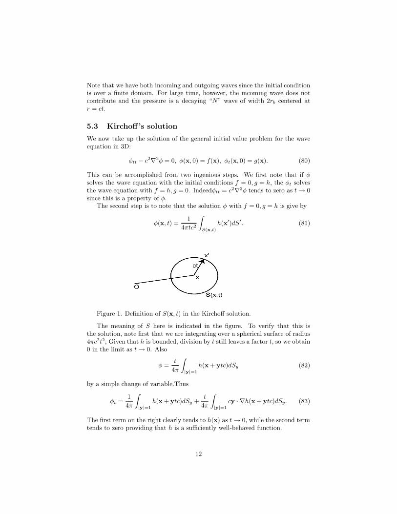
The second step is to note that the solution φ with f = 0, g = h is give by
φ(x, t) =1
4πtc2
∫
S(x,t)
h(x′)dS′. (81)
Figure 1. Definition of S(x, t) in the Kirchoff solution.
The meaning of S here is indicated in the figure. To verify that this isthe solution, note first that we are integrating over a spherical surface of radius4πc2t2, Given that h is bounded, division by t still leaves a factor t, so we obtain0 in the limit as t → 0. Also
φ =t
4π
∫
|y|=1
h(x + ytc)dSy (82)
by a simple change of variable.Thus
φt =14π
∫
|y|=1
h(x + ytc)dSy +t
4π
∫
|y|=1
cy · ∇h(x + ytc)dSy. (83)
The first term on the right clearly tends to h(x) as t → 0, while the second termtends to zero providing that h is a sufficiently well-behaved function.
12
We now show that (82) solves the wave equation. Using the divergencetheorem we can write (83) in the form
φt =14π
∫
|y|=1
h(x + ytc)dSy +1
4πct
∫
V (x,t)
∇2h(x′)dV ′, (84)
where V (x, t) denotes the sphere of radiuc ct centered at x. Then
φt =14π
∫
|y|=1
h(x + ytc)dSy +1
4πct
∫ ct
0
∫
Sρ(x)
∇2h(y)dSydρ, (85)
where Sρ(x) is the spherical surface of radius ρ centered at x.Now we can compute
φtt =c
4π
∫
|y|=1
y·∇h(x+ytc)dSy−1
4πct2
∫
V (x,t)
∇2h(x′)dV ′+1
4πt
∫
S(x,t)
∇2h(y)dSy
=1
4πct2
∫
V (x,t)
∇2h(x′)dV ′− 14πct2
∫
V (x,t)
∇2h(x′)dV ′+1
4πt
∫
S(x,t)
∇2h(y)dSy
=1
4πt
∫
S(x,t)
∇2h(y)dSy.
=c2t
4π
∫
|y|=1
h(x + ytc)dSy = c2∇2φ. (86)
Thus we have shown that φ satisfies the wave equation.Given these facts we may write down Kirchoff’s solution to the initial value
problem with initial data f, g:
φ(x, t) =1
4πtc2
∫
S(x,t)
g(x′)dS′ +∂
∂t
14πtc2
∫
S(x,t)
f(x′)dS′. (87)
Although we have seen that the domain of dependence of a point in spaceat a future time is in fact a finite segment of the line in one dimension, thecorresponding statement in 3D, that the domain of dependence is a finite regionof 3-space, is false. The actual domain of dependence is the surface of a sphereof radius ct, centered at x. This fact is know as Huygen’s principle.
We note that the bursting balloon problem can be solved directly using theKirchoff formula. A nice exercise is to compare this method with the 1D solutionwe gave above.
Moving sound sources give rise to different sound field depending uponwhether or not the source is moving slower of faster that the speed of sound. Inthe latter case, a source moving to the left along the x-axis with a speed U > cwill produce sound waves having a conical envelope, see figure 2.
13
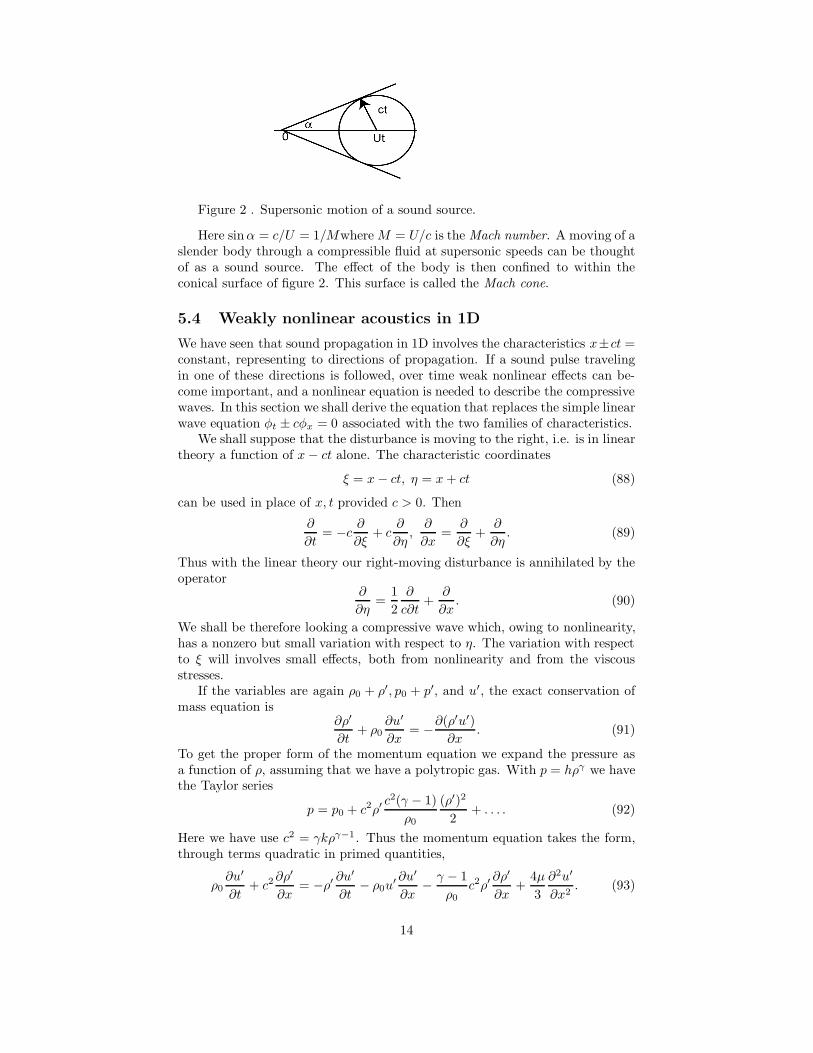
Figure 2 . Supersonic motion of a sound source.
Here sinα = c/U = 1/Mwhere M = U/c is the Mach number. A moving of aslender body through a compressible fluid at supersonic speeds can be thoughtof as a sound source. The effect of the body is then confined to within theconical surface of figure 2. This surface is called the Mach cone.
5.4 Weakly nonlinear acoustics in 1D
We have seen that sound propagation in 1D involves the characteristics x±ct =constant, representing to directions of propagation. If a sound pulse travelingin one of these directions is followed, over time weak nonlinear effects can be-come important, and a nonlinear equation is needed to describe the compressivewaves. In this section we shall derive the equation that replaces the simple linearwave equation φt ± cφx = 0 associated with the two families of characteristics.
We shall suppose that the disturbance is moving to the right, i.e. is in lineartheory a function of x− ct alone. The characteristic coordinates
ξ = x− ct, η = x+ ct (88)
can be used in place of x, t provided c > 0. Then
∂
∂t= −c ∂
∂ξ+ c
∂
∂η,∂
∂x=
∂
∂ξ+
∂
∂η. (89)
Thus with the linear theory our right-moving disturbance is annihilated by theoperator
∂
∂η=
12∂
c∂t+
∂
∂x. (90)
We shall be therefore looking a compressive wave which, owing to nonlinearity,has a nonzero but small variation with respect to η. The variation with respectto ξ will involves small effects, both from nonlinearity and from the viscousstresses.
If the variables are again ρ0 + ρ′, p0 + p′, and u′, the exact conservation ofmass equation is
∂ρ′
∂t+ ρ0
∂u′
∂x= −∂(ρ
′u′)∂x
. (91)
To get the proper form of the momentum equation we expand the pressure asa function of ρ, assuming that we have a polytropic gas. With p = hργ we havethe Taylor series
p = p0 + c2ρ′c2(γ − 1)
ρ0
(ρ′)2
2+ . . . . (92)
Here we have use c2 = γkργ−1. Thus the momentum equation takes the form,through terms quadratic in primed quantities,
ρ0∂u′
∂t+ c2
∂ρ′
∂x= −ρ′ ∂u
′
∂t− ρ0u
′ ∂u′
∂x− γ − 1
ρ0c2ρ′
∂ρ′
∂x+
4µ3∂2u′
∂x2. (93)
14
Note that the viscous stress term comes from the difference 2µ − 23µ in the
coefficient of ∂u′
∂xin the 1D stress tensor. We assume here that µ is a constant.
To derive a nonlinear equation for the propagating disturbance we proceedin two steps. First, eliminate the ξ differentiations from the linear parts of thetwo equations. This will yield a equation with a first derivative term in η, alongwith the viscosity term and a collection of quadratic nonlinearities in u′, ρ′.Then we use the approximate linear relation between u′ and ρ′ to eliminate ρ′
in favor of u′ in these terms. The result will be a nonlinear equation for u′ inwill all terms are small but comparable.
The linear relation used in the nonlinear terms comes from
ρ0∂u′
∂t= −c2 ∂ρ
′
∂x(94)
Since dependence upon η is weak, the last relation expressed in ξ, η variablesbecomes
−cρ0∂u′
∂ξ= −c2 ∂ρ
′
∂ξ, (95)
so thatρ′ ≈ ρ0
cu′ (96)
in the nonlinear terms as well as in any derivative with respect to η.Now in characteristic coordinates the linear parts of the equations take the
forms∂
∂ξ(−cρ′ + ρ0u
′) +∂
∂η(cρ′ + ρ0u
′) = −∂(ρ′u′)∂x
. (97)
∂
∂ξ(−cρ0u
′ + c2ρ′) +∂
∂η(cρ0u
′ + c2ρ′) = . . . , (98)
where the RHS consists of nonlinear and viscous terms. Dividing the second ofthese by c and adding the two equations we get
2∂
∂η(cρ′+ρ0u
′) = −∂(ρ′u′)∂x
− 1cρ′∂u′
∂t− ρ0
cu′∂u′
∂x− γ − 1
ρ0cρ′
∂ρ′
∂x+
4µ3c∂2u′
∂x2. (99)
Since the LHS here involves now only the ηderivative, we may use (96) toeliminate ρ′, and similarly with all terms on the RHS. Also we express x and tderivatives on the RHS in terms of ξ. Thus we have
4ρ0∂u′
∂η= −2
ρ0
cu′∂u′
∂ξ+ρ0
cu′∂u′
∂ξ− +
ρ0
cu′∂u′
∂ξ− (γ − 1)ρ0
cu′∂u′
∂ξ+
4µ3c∂2u′
∂ξ2.
(100)Thus
2c∂u′
∂η+γ + 1
2u′∂u′
∂ξ− 2µ
3ρ0
∂2u′
∂ξ2= 0. (101)
Now∂
∂η=
12c
( ∂∂t
+ c∂
∂x
), (102)
15
so∂u′
∂t|x + c
∂u′
∂x|t +
γ + 12
u′∂u′
∂ξ−
2µ3ρ0
∂2u′
∂ξ2= 0. (103)
Now this involves a linear operator describing the time derivative relative to anobserver moving with the speed c. The linear operator is now the time derivativeholding ξ fixed. Thus
∂u′
∂t|ξ +
γ + 12
u′∂u′
∂ξ− 2µ
3ρ0
∂2u′
∂ξ2= 0. (104)
The velocity perturbation u′, we emphasize, is that relative to the fluid at restat infinity. Moving with the wave the gas is seen to move with velocity u = u′−cor u′ really denotes u+ c where u is the velocity seen by the moving observer.
What we have in (104) is the viscous form of Burgers’ equation. It is anonlinear wave equation incorporating viscous dissipation but not dispersion.By suitable scaling it may be brought into the form
ut + uux − νuxx = 0. (105)
If the viscous term is dropped we have the inviscid Burgers wave equation,
ut + uux = 0. (106)
This equation is much studied as a prototypical nonlinear wave equation. Wereview the method of characteristics for such equations in the next section.
6 Nonlinear waves in one dimension
The simplest scalar wave equation can be written in the conservation form
∂u
∂t+
∂
∂xF (u) = 0, (107)
equivalent to∂u
∂t+ v(u)
∂u
∂x= 0, v(u) = F ′(u). (108)
The last equation can be regarded as stating that an observer moving with thevelocity v(u) observes that u does not change. The particle path of the observeris called a characteristic curve. Since u is constant on the characteristic and thevelocity v is a function of u alone we see that the characteristic is a straight linein the x, t- plane. If u(x, 0) = u0(x), the characteristics are given by the family
x = v(u0(x0))t + x0. (109)
Here x0 acts like a Lagrangian coordinate, marking the intersection of the char-acteristic with the initial line t = 0.
16
As an example of the solution of the initial-value problem using character-istics, consider the equation
∂u
∂t+ u2∂u
∂x= 0, u0(x) =
{ 0, if x < 0,x, if 0 < x < 1,1, if x > 1
. (110)
First observe that the characteristics are vertical line in x < 0, so that u = 0 inx < 0, t > 0. Similarly the characteristics are the line x = t + x0 when x0 > 1,so that u = 1 when x > 1 + t. Solving x = x2
0t+x0 for x0(x, t), we arrive at thefollowing solution in the middle region 0 < x < 1 + t:
u(x, t) =−1 +
√1 + 4xt
2t. (111)
Now we modify the initial condition to
u0(x) =
{ 0, if x < 0,x/ε, if 0 < x < ε,1, if x > ε
. (112)
The solution is then, since the characteristics in the middle region are x =(x0/ε)2t+ x0
u(x, t) =ε
2t
[−1 +
√1 + 4xt/ε2
]. (113)
letting ε→ 0 in (113) we obtain
u→√x
t. (114)
This solution, existing in the wedge 0 < x/t < 1 of the x, t-plane, is called anexpansion fan. Given the discontinuous initial condition
u ={
0, if x < 0,1, if x > 0, (115)
we can solve for the expansion fan directly by noting that u must be a functionof η = x/t Substituting u = f(η) in our equation, we obtain
−ηf ′ + f2f ′ = 0, (116)
implying f = ±√η. The positive sign is needed to make the solution continuous
at the edges of the fan.
6.1 Dynamics of a polytropic gas
We have the following equation for a polytropic gas in one dimension, in theabsence of dissipative processes and assuming constant entropy:
ut + uux +c2
ρρx, ρt + uρx + ρux = 0. (117)
17
Here c2 = kγργ−1. If we define the column vector [u ρ]T = w, the system maybe written wt +A ·wx where
A =(u c2/ρρ u
). (118)
We now try to find analogs of the characteristic lines x ± ct = constant whicharose in acoustics in one space dimension. We want to find curves on whichsome physical quantity is invariant. Suppose that v is a right eigenvector of AT
(transpose of A), AT · v = λv. We want to show that the eigenvalue λ plays arole analogous to the acoustic sound velocity.
Indeed, we see that
vT · [wt + A ·wx] = vT ·wt +AT · v ·wx = vT ·wt + λvT ·wx = 0. (119)
Now suppose that we can find an integrating factor φ such that φvT · dw = dF .The we would have
Ft + λFx = 0. (120)
Thus dx/dt = λ would define a characteristic curve in the x, t- plane on whichF = constant. The quantity F is called a Riemann invariant.
Thus we solve the eigenvalue equation
det(AT − λI) =∣∣∣(u− λ ρc2/ρ u− λ
)∣∣∣ = 0. (121)
Then (u− λ)2 = c2, orλ = u± c ≡ λ±. (122)
We see that the characteristic speeds are indeed related to sound velocity, butnow altered by the doppler shift introduced by the fluid velocity. (Unlike lightthrough space, the speed of sound does depend upon the motion of the observer.Sound moves relative to the compressible fluid in which it exists.)
Thus the following eigenvectors are obtained:
λ+ :(
−c ρc2/ρ −c
)v+ = 0, vT
+ = [ρ c], (123)
λ− :(
c ρc2/ρ c
)v− = 0, vT
− = [ρ − c], (124)
We now choose φ:
φ[ρ ± c][dudρ
]= dF±. (125)
Since c is a function of ρ we see that we may take φ = 1/ρ, to obtain
F± = u±∫
c
ρdρ, (126)
18
which may be brought into the form
F± = u± 2γ − 1
c. (127)
Thus we find that the Riemann invariants u± 2γ−1
c are constant on the curvesdxdt = u± c: [ ∂
∂t+ (u± c)
∂
∂x
][u± 2
γ − 1c]
= 0. (128)
6.2 Simple waves
Any region of the x, t-plane which is adjacent to a region where are fluid variablesare constant (i.e. a region at a constant state), but which is not itself a region ofconstant state, will be called a simple wave region, or SWR. The characteristicfamilies of curves associated with λ± will be denoted by C±. Curves of bothfamilies will generally propagate through a region. In a simple wave region onefamily of characteristics penetrates into the region of constant state, so that oneof the two invariants F± will be known to be constant over a SWR. Supposethat F− is constant over the SWR. Then any C+ characteristic in the SWRnot only carries a constant value of F+ but also a constant value of F−, andthis implies a constant value of u + c (see the definitions (127) of F±). Thusin a SWR where F− is constant the C+ characteristics are straight lines, andsimilarly for the C− characteristics over a SWR where F+ is constant.
Let us suppose that a simple wave region involving constant F− involves u >0, so fluid particles move upward in the x, t-plane. All of the C+ characteristicshave positive slope. They may either converge on diverge. In the latter case wehave the situation shown in figure 3(a). Since u+c > u, fluid particles must crossthe C+ characteristics from right to left. Moving along this path, a fluid particleexperiences steadily decreasing values of u+c. We assume now that γ > 1. Sinceu = 2c
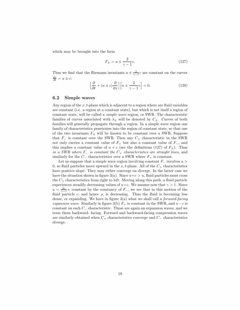
γ−1+ constant by the constancy of F−, we see that in this motion of thefluid particle c, and hence ρ, is decreasing. Thus the fluid is becoming lessdense, or expanding. We have in figure 3(a) what we shall call a forward-facingexpansion wave. Similarly in figure 3(b) F+ is constant in the SWR, and u−c isconstant on each C− characteristic. These are again an expansion waves, and weterm them backward- facing. Forward and backward-facing compression wavesare similarly obtained when C+ characteristics converge and C− characteristicsdiverge.
19
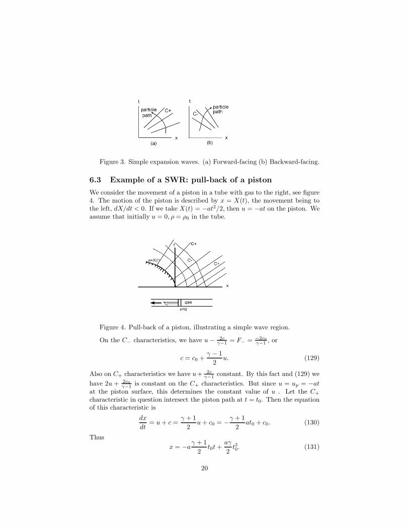
Figure 3. Simple expansion waves. (a) Forward-facing (b) Backward-facing.
6.3 Example of a SWR: pull-back of a piston
We consider the movement of a piston in a tube with gas to the right, see figure4. The motion of the piston is described by x = X(t), the movement being tothe left, dX/dt < 0. If we take X(t) = −at2/2, then u = −at on the piston. Weassume that initially u = 0, ρ = ρ0 in the tube.
Figure 4. Pull-back of a piston, illustrating a simple wave region.
On the C− characteristics, we have u− 2cγ−1 = F− = −2c0
γ−1 , or
c = c0 +γ − 1
2u. (129)
Also on C+ characteristics we have u+ 2cγ−1 constant. By this fact and (129) we
have 2u + 2c0γ−1 is constant on the C+ characteristics. But since u = up = −at
at the piston surface, this determines the constant value of u . Let the C+
characteristic in question intersect the piston path at t = t0. Then the equationof this characteristic is
dx
dt= u+ c =
γ + 12
u+ c0 = −γ + 12
at0 + c0. (130)
Thusx = −aγ + 1
2t0t+
aγ
2t20. (131)
20
If we solve the last equation for t0(X,T ) we obtain
t0 =1aγ
[at(γ + 1)2
+
√(at(γ + 1)
2)2 + 2xaγ
]. (132)
Then u = −at0(x, t) in the simple wave region, c being given by (129).Note that according to (129), c = 0 when t = t∗, where at∗ = 2
γ−1c0. This
piston speed is the limiting speed the gas can obtain. For t > t∗ the piston pullsaway from a vacuum region bounded by an interface moving with speed −at∗.
If we consider the case of instantaneous motion of the velocity with speedup, the C+ characteristics emerge from the origin as an expansion fan. Theirequation is
x
t= u+ c = c0 +
γ + 12
u, (133)
so thatu =
2γ + 1
[xt− 2c0
]. (134)
To compute the paths ξ(t) of fluid particles in this example, we must solve
dξ
dt=
2γ + 1
[ξt− 2c0
]. (135)
A particle begins to move with the rightmost wave of the expansion fan, namelythe line x = c0t, meets the initial particle position. Thus (135) must be solvedwith the initial condition ξ(t0) = c0t0. The solution is
ξ(t) =−2c0γ − 1
t+ c0t0γ + 1γ − 1
(t/t0)2
γ+1 . (136)
For the location of the C− characteristics we must solve
dx
dt= u− c =
3 − γ
2u− c0 =
3 − γ
γ + 1(x/t− c0) − c0, (137)
with the initial condition x(t0) = c0t0. There results
x(t) =−2c0γ − 1
t+ c0t0γ + 1γ − 1
(t/t0)3−γ1−γ . (138)
7 Linearized supersonic flow
We have seen above that 2D irrotational inviscid homentropic flow of a poly-tropic gas satisfies the system
(c2 − φ2x)φxx + (c2 − φ2
y)φyy − 2φxφy∇2φ = 0, (139)
φ2x + φ2
y +2
γ − 1c2 = constant. (140)
21
We are interested in the motion of thin bodies which do not disturb the ambientfluid very much, The assumption of small perturbations, and the correspondinglinearized theory of compressible flow, allows us to consider some steady flowproblems of practical interest which are analogs of sound propagation problems.
We assume that the air moves with a speed U past the body, from left toright in the direction of the x-axis. Then the potential is taken to have the form
φ = U0x+ φ′, (141)
where |φ′x| � U0. It is easy to derive the linearized form of (139), since the
second-derivative terms must be primed quantities. The other factors are thenevaluated at the ambient conditions, c ≈ c0, φx ≈ U). Thus we obtain
(M2 − 1)φ′xx − φ′
yy. (142)
HereM = U0/c0 (143)
is the Mach number of the ambient flow. We note that in the linear theory thepressure is obtained from
U0∂u′
∂x+
1ρ0
∂p′
∂x, (144)
orp′ ≈ −U0ρ0φ
′x. (145)
We now drop the prime from φ′. The density perturbation is then ρ′ = −c−20 U0ρφx.
22
7.1 Thin airfoil theory
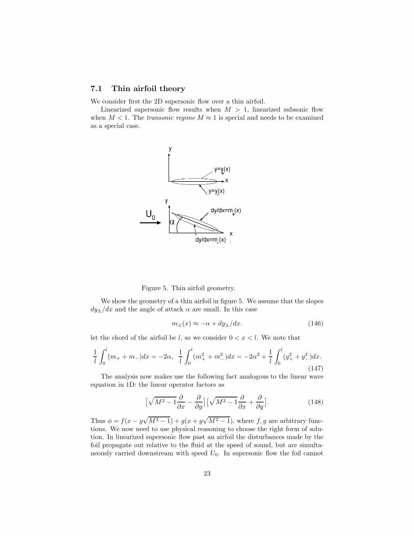
We consider first the 2D supersonic flow over a thin airfoil.Linearized supersonic flow results when M > 1, linearized subsonic flow
when M < 1. The transonic regime M ≈ 1 is special and needs to be examinedas a special case.
Figure 5. Thin airfoil geometry.
We show the geometry of a thin airfoil in figure 5. We assume that the slopesdy±/dx and the angle of attack α are small. In this case
m±(x) ≈ −α+ dy±/dx. (146)
let the chord of the airfoil be l, so we consider 0 < x < l. We note that
1l
∫ l
0
(m+ +m−)dx = −2α,1l
∫ l
0
(m2+ +m2
−)dx = −2α2 +1l
∫ l
0
(y2+ + y2
−)dx.
(147)The analysis now makes use the following fact analogous to the linear wave
equation in 1D: the linear operator factors as
[√M2 − 1
∂
∂x− ∂
∂y
][√M2 − 1
∂
∂x+
∂
∂y
]. (148)
Thus φ = f(x − y√M2 − 1) + g(x+ y
√M2 − 1), where f, g are arbitrary func-
tions. We now need to use physical reasoning to choose the right form of solu-tion. In linearized supersonic flow past an airfoil the disturbances made by thefoil propagate out relative to the fluid at the speed of sound, but are simulta-neously carried downstream with speed U0. In supersonic flow the foil cannot
23
therefore cause disturbances of the fluid upstream of the body. Consequently thecharacteristic lines x ± y
√M2 − 1 = constant, which carry disturbances away
from the foil, must always point downstream. Thus in the half space above thefoil the correct choice is φ = f(x − y
√M2 − 1), while in the space below it the
correct choice is φ = g(x+ y√M2 − 1). To determine these functions, we must
make the flow tangent to the foil surface. Since we are dealing with thin airfoilsand small angles, the condition of tangency can be applied, approximately, aty = 0. Thus we have the tangency conditions
φy
U0|y=0+ = m+(x) = −
√M2 − 1U−1
0 f ′(x), (149)
φy
U0|y=0− = m−(x) =
√M2 − 1U−1
0 g′(x), (150)
Of interest to engineers is the lift and drag of a foil. To compute these wefirst need the pressures
p′+(x) = −U0ρ0u′(x, 0+) = −U0ρ0f
′(x), p′−(x) = −U0ρ0g′(x). (151)
This yields
p′± = ± U20 ρ0√
M2 − 1(−α+ dy±/dx). (152)
Then
Lift =∫ l
0
(p′− − p′+)dx =2αρ0U
20 l√
M2 − 1, (153)
Drag =∫ l
0
(p′+m+−p′−m−)dx =ρ0U
20 l√
M2 − 1[2α2+
1l
∫ l
0
[(dy+/dx)2+(dy−/dx)2]dx.
(154)Note that now inviscid theory gives a positive drag. We recall that for
incompressible potential flow we obtained zero drag (D’Alembert’s paradox).In supersonic flow, the characteristics carry finite signals to infinity. In fact thedisturbances are being created so that the rate of increase of kinetic energy perunit time is just equal to the drag times U0. This drag is often called wave dragbecause it is associated with characteristics, usually called in this context Machwaves, which propagate to infinity.
What happens if we solve for compressible flow past a body in the subsoniccase M < 1? In the case of thin airfoil theory, it is easy to see that we mustget zero drag. The reason is that the equation we are now solving may bewritten φxx + φyy = 0 where y =
√1 −M2y. The boundary conditions are at
y = y = 0 so in the new variables we have a problem equivalent to that of anincompressible potential flow.
In fact compressible potential flow past any finite body will give zero dragso long as the flow field velocity never exceeds the local speed of sound, i.e. thefluid stays locally subsonic everywhere. In that case no shock waves can form,there is no dissipation, and D’Alembert’s paradox remains.
24
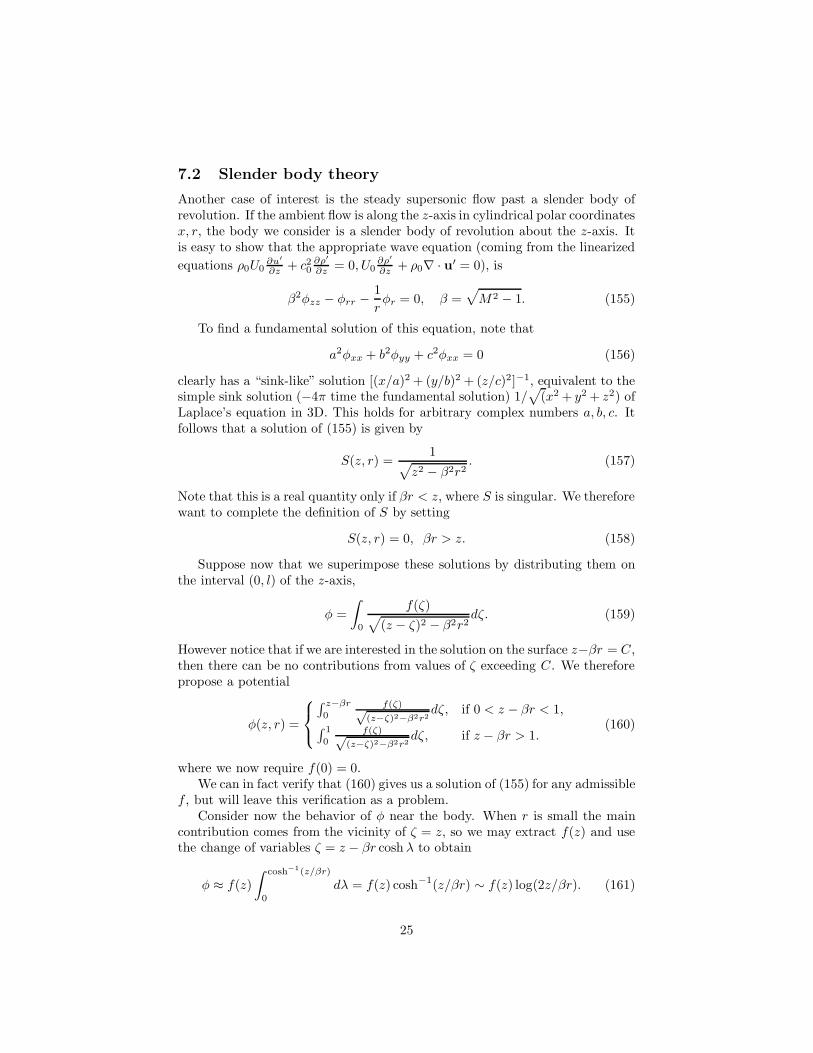
7.2 Slender body theory
Another case of interest is the steady supersonic flow past a slender body ofrevolution. If the ambient flow is along the z-axis in cylindrical polar coordinatesx, r, the body we consider is a slender body of revolution about the z-axis. Itis easy to show that the appropriate wave equation (coming from the linearizedequations ρ0U0
∂u′
∂z + c20∂ρ′
∂z = 0, U0∂ρ′
∂z + ρ0∇ · u′ = 0), is
β2φzz − φrr −1rφr = 0, β =
√M2 − 1. (155)
To find a fundamental solution of this equation, note that
a2φxx + b2φyy + c2φxx = 0 (156)
clearly has a “sink-like” solution [(x/a)2 + (y/b)2 + (z/c)2]−1, equivalent to thesimple sink solution (−4π time the fundamental solution) 1/
√(x2 + y2 + z2) of
Laplace’s equation in 3D. This holds for arbitrary complex numbers a, b, c. Itfollows that a solution of (155) is given by
S(z, r) =1√
z2 − β2r2. (157)
Note that this is a real quantity only if βr < z, where S is singular. We thereforewant to complete the definition of S by setting
S(z, r) = 0, βr > z. (158)
Suppose now that we superimpose these solutions by distributing them onthe interval (0, l) of the z-axis,
φ =∫
0
f(ζ)√(z − ζ)2 − β2r2
dζ. (159)
However notice that if we are interested in the solution on the surface z−βr = C,then there can be no contributions from values of ζ exceeding C. We thereforepropose a potential
φ(z, r) =
∫ z−βr
0f(ζ)√
(z−ζ)2−β2r2dζ, if 0 < z − βr < 1,
∫ 1
0f(ζ)√
(z−ζ)2−β2r2dζ, if z − βr > 1.
(160)
where we now require f(0) = 0.We can in fact verify that (160) gives us a solution of (155) for any admissible
f , but will leave this verification as a problem.Consider now the behavior of φ near the body. When r is small the main
contribution comes from the vicinity of ζ = z, so we may extract f(z) and usethe change of variables ζ = z − βr cosh λ to obtain
φ ≈ f(z)∫ cosh−1(z/βr)
0
dλ = f(z) cosh−1(z/βr) ∼ f(z) log(2z/βr). (161)
25
Now let the body be described by r = R(z), 0 < z < l. The tangencycondition is then
rφr
U0
∣∣∣r=R
= RdR
dz≈ −f(z)/U0 . (162)
If A(a) denotes cross-sectional area, then we have
f(z) = − 12πU0dA
dz. (163)
Figure 6. Steady supersonic flow past a slender body of revolution. Heretanα = 1/
√M2 − 1.
The calculation of drag is a bit more complicated here, and we give the resultfor the case where R(0) = R(l) = 0. Then
Drag =ρ0U
20
4π
∫ l
0
∫ l
0
A′′(z)A′′(ζ)1
log |z − ζ|dzdζ. (164)
The form of this emphasizes the importance of having a smooth distribution ofarea in order to minimize drag.
7.2.1 An alternative formulation and proof of the drag formula
To prove (164) it is convenient to reformulate the problem in terms of a stream-function. We go back to the basic equations for steady homentropic potentialflow in cylindrical polar coordinates.
∂ur
∂z− ∂uz
∂r= 0,
∂rρuz
∂z+∂rρur
∂r= 0, (165)
u2z + u2
r +2
γ − 1c2 = constant. (166)
26
From the second of (165) we introduce the streamfunction ψ,
rρuz =∂ψ
∂r, rρur = −∂ψ
∂z. (167)
We then expand the equations as follows:
ψ =U0
2r2 + ψ′, ρ = ρ0 + ρ′, (168)
and linearize. The result is the equation for ψ′,
r∂
∂r
1r
∂ψ′
∂r− β2 ∂
2ψ′
∂z2= 0. (169)
Now the boundary condition in terms of the stream function is that ψ equalzero on the slender body r = R(z). Approximately, this gives
ρ0U0
2r2 + ψ′(z, 0) ≈ 0. (170)
We also want no disturbance upstream, so ψ′ and ′′z should vanish on z =0, r > 0. A solution of this problem is given by
ψ′ ={−ρ0U0
2π
∫ z−βr
0
√(z − ζ)2 − β2r2A′′dζ, if z ≥ βr,
0, if z < βr.(171)
It is easy to see that the equation and upstream conditions are satisfiedunder the conditions that R(0) = 0. For the boundary condition we have
ψ′(z, 0) = −ρ0U0
2π
∫ z
0
(z − ζ)A′′dζ = −ρ0U0
2π
∫ z
0
A′dζ = −ρ0U0
2R2. (172)
Now the drag is given by
D =∫ l
0
p′A′(ζ)dζ, (173)
where the linear theory gives p′ ≈ −ρ0U0u′z. However it turns out that the ur
velocity components become sufficiently large near the body to make a leadingorder contribution. Thus we have
p′ ≈ −ρ0U0u′z −
ρ0
2(u′r)
2 + . . . . (174)
We note thatu′z =
( 1ρr
∂ψ
∂r
)′≈ 1ρ0r
∂ψ′
∂r− U0
ρ0c20p′, (175)
from which we have−β2u′z =
1ρ0r
∂ψ′
∂r. (176)
27

Thus
u′z = −U0
2π
∫ z−βr
0
A′′(ζ)√(z − ζ)2 − β2r2
dζ. (177)
Similarly
u′r =U0
2πr
∫ z−βr
0
(z − ζ)A′′(ζ)√
(z − ζ)2 − β2r2dζ. (178)
We see by letting r → R ≈ 0 in (178) that
u′r ≈ U0
2πA′(z)/R(z). (179)
Also
u′z ≈ −U0
2π
[A′′(z − βr) cosh−1 z
βr+
∫ z−βr
0
A′′(ζ) −A′′(z − βr)√(z − ζ)2 − β2r2
dζ]
(180)
≈ −U0
2π
[A′′ log
2zβR
−∫ z
0
A′′(z) − A′′(ζ)z − ζ
dζ]. (181)
We are now in a position to compute D:
D =ρ0U
20
2π
∫ l
0
A′(z)∫ z−βR
0
[A′′(z) log
2zβr
−∫ z
0
A′′(z) − A′′(ζ)z − ζ
dζ−14A−1(z)(A′)2(z)
]dz.
(182)After an integration by parts and a cancelation we have
D =ρ0U
20
2π
∫ l
0
A′(z)[A′′(z) log z −
∫ z
0
A′′(z) − A′′(ζ)z − ζ
dζ]dz. (183)
Our last step is to show that (183) agrees with (164). Now if B(z) = A′(z),∫ l
0
∫ l
0
B′(z)B′(ζ) log |z − ζ|dζdz = 2∫ l
0
B′(z)∫ z
0
B′(ζ) log |z − ζ|dζdz
= 2∫ l
0
B′(z)B(z) log zdz + 2∫ l
0
B′(z)∫ z
0
B(z) −B(ζ)z − ζ
dζdz
= −2∫ l
0
B′(z)B(z) log zdz − 2∫ l
0
B(z)∫ z
0
B′(z) −B′(ζ)z − ζ
dζdz, (184)
which proves the agreement of the two expressions. Here we have used
d
dz
∫ z
0
B(z) −B(ζ)z − ζ
dζ =B(z) −B(ζ)
z − ζ
∣∣∣ζ
= z+∫ z
0
(z − ζ)B′(z) −B(z) + B(ζ)(z − ζ)2
dζ
= B′(z) +[ (z − ζ)b′(z) − B(z) + B(ζ)
(z − ζ)2]z
0+
∫ z
0
B′(z) − B(ζ)z − ζ
dζ
=∫ z
0
B′(z) −B′(ζ)z − ζ
dζ + B(z)/z. (185)
28
8 Shock waves
8.1 Scalar case
We have seen that the equation ut + uux = 0 with a initial condition u(x, 0) =1 − x on the segment 0 < x < 1 produces a family of characteristics
x = (1 − x0)t+ x0. (186)
This family of lines intersects at (x, t) = (1, 1). If the initial condition is ex-tended as
u(x, 0) ={
1, if x < 0,0, if x > 1, (187)
we see that at t = 1 a discontinuity develops in u as a function of x. Wethus need to study how such discontinuities propagate for later times as shockwaves. We study first the general scalar wave equation in conservation form,ut + (F (u))x = 0. This equation is assumed to come from a conservation law ofthe form
d
dt
∫ b
a
udx = F (u(a, t))− F (u(b, t)). (188)
Suppose now that in fact there is a discontinuity present at position ξ(t) ∈(a, b). Then we study the conservation law by breaking up the interval so thatdifferentiation under the integral sign is permitted:
d
dt
[ ∫ ξ
a
udx+∫ b
ξ
udx]
= F (u(a, t))− F (u(b, t)). (189)
Now differentiating under the integral and using the wave equation to eliminatethe time derivatives of u we obtain
dξ
dt[u(ξ+, t) − u(ξ−, t)] = F (u(ξ+, t)) − F (u(ξ−, t)). (190)
Thus we have an expression for the propagation velocity of the shock wave:
dξ
dt=
[F ]x=ξ
[u]x=ξ, (191)
where here [·] means “jump in”. The direction you take the jump is immaterialprovided that you do the same in numerator and denominator.
Example: Let ut + uux = 0,
u(x, 0) =
0, if x < −1,1 + x, if −1 < x < 0,1 − 2x, if 0 < x < 1/2.
(192)
The characteristic family associated with the interval −1 < x < 0 is x =(1 +x0)t+ x0, while that of 0 < x < 1/2 is x = (1− 2x0)t+ x0. The shock first
29
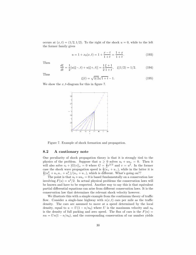
occurs at (x, t) = (1/2, 1/2). To the right of the shock u = 0, while to the leftthe former family gives
u = 1 + x0(x, t) = 1 +x− t
1 + t=
1 + x
1 + t. (193)
Thendξ
dt=
12[u(ξ−, t) + u(ξ+, t)] =
12ξ + 11 + t
, ξ(1/2) = 1/2. (194)
Thusξ(t) =
√3/2
√1 + t− 1. (195)
We show the x, t-diagram for this in figure 7.
Figure 7. Example of shock formation and propagation.
8.2 A cautionary note
One peculiarity of shock propagation theory is that it is strongly tied to thephysics of the problem. Suppose that u ≥ 0 solves ut + uux = 0. Then itwill also solve vt + [G(v)]x = 0 where G = 2
3v3/2 and v = u2. In the former
case the shock wave propagation speed is 12(u+ + u−), while in the latter it is
23(u2
+ + u+u− + u2−)/(u+ + u−), which is different. What’s going on??
The point is that ut +uux = 0 is based fundamentally on a conservation lawinvolving F (u) = u2/2. In actual physical problems the conservation laws willbe known and have to be respected. Another way to say this is that equivalentpartial differential equations can arise from different conservation laws. It is theconservation law that determines the relevant shock velocity however.
We illustrate this with a simple example from the continuum theory of trafficflow. Consider a single-lane highway with n(x, t) cars per mile as the trafficdensity. The cars are assumed to move at a speed determined by the localdensity, equal to u = U (1 − n/n0) where U is the maximum velocity and n0
is the density of full packing and zero speed. The flux of cars is the F (n) =nu = Un(1 − n/n0), and the corresponding conservation of car number yields
30
the PDE nt + [F (n)]x = 0. This is equivalent to vt + [G(v)]x = 0 where v = n2
and G = U [v − 23n0
v3/2]. However the conservation law associated with v,Gmakes no physical sense. We know how the speed of the cars depends uponn, and conservation of number (if indeed that is what happens) dictates theformer conservation law. Note that if the square of density was somehow whatwas important in the conservation of mass, we would end up with a conservationof mass equation ∂ρ2
∂t+ ∇ · (ρ2u) = 0.
8.3 The stationary normal shock wave in gas dynamics
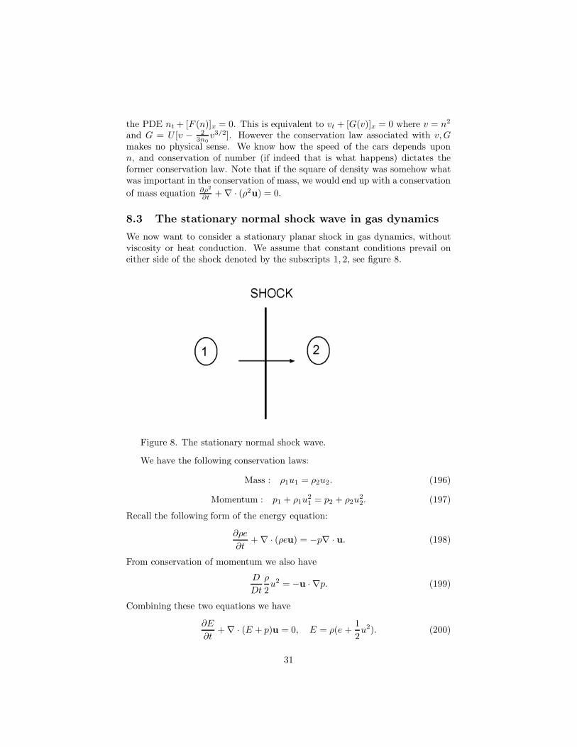
We now want to consider a stationary planar shock in gas dynamics, withoutviscosity or heat conduction. We assume that constant conditions prevail oneither side of the shock denoted by the subscripts 1, 2, see figure 8.
Figure 8. The stationary normal shock wave.
We have the following conservation laws:
Mass : ρ1u1 = ρ2u2. (196)
Momentum : p1 + ρ1u21 = p2 + ρ2u
22. (197)
Recall the following form of the energy equation:
∂ρe
∂t+ ∇ · (ρeu) = −p∇ · u. (198)
From conservation of momentum we also have
D
Dt
ρ
2u2 = −u · ∇p. (199)
Combining these two equations we have
∂E
∂t+ ∇ · (E + p)u = 0, E = ρ(e +
12u2). (200)
31
At the shock we must therefore require continuity of (ρu(e+ pρ + 1
2u2), and since
ρu is continuous we have that e+ pρ + 1
2u2 = h+ 1
2u2 is continuous:
Energy : h1 +12u2
1 = h2 +12u2
2. (201)
Let us write m = ρu as the constant mass flux, and let v = 1/ρ. Thenconservation of energy may be rewritten
h2 − h1 =12m2(v2
1 − v22). (202)
Also conservation of momentum can be rewritten
m2 =p1 − p2
v2 − v1(203)
Thush1 − h2 =
12(v1 + v2)m2(v2 − v1), (204)
which is equivalent to
h1 − h2 =12(v1 + v2))p1 − p2). (205)
Written out, this means
e1 − e2 + p1v1 − p2v2 =12(v1 + v2))p1 − p2) (206)
ore1 − e2 =
12(v2 − v1)(p1 + p2). (207)
The relations (205),(207) involving the values of the primitive thermodynamicquantities on either side of the shock are called the Rankine-Hugoniot relations.
For a polytropic gas we have
e =1
γ − 1pv. (208)
This allows us to write (207) as
2γ − 1
(p1v1 − p2v2) + (v1 − v2)(p1 + p2) = 0, (209)
orγ + 1γ − 1
(p1v1 − p2v2) − v2p1 + p2v1 = 0. (210)
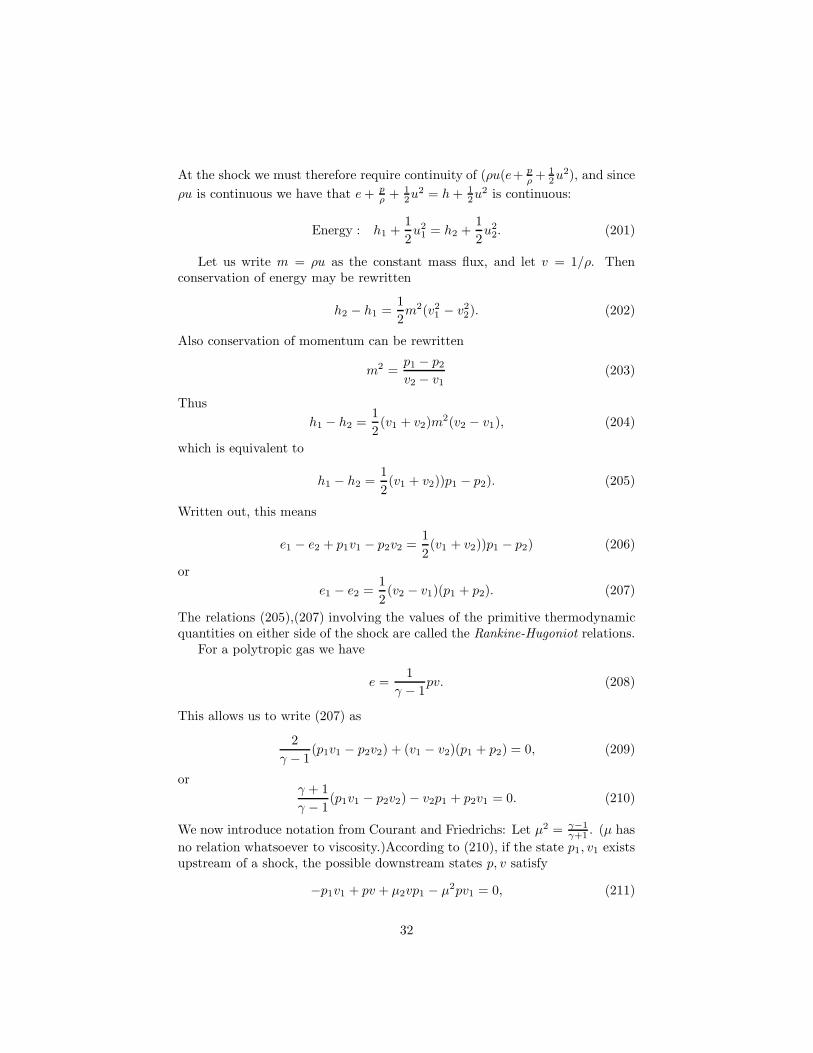
We now introduce notation from Courant and Friedrichs: Let µ2 = γ−1γ+1 . (µ has
no relation whatsoever to viscosity.)According to (210), if the state p1, v1 existsupstream of a shock, the possible downstream states p, v satisfy
−p1v1 + pv + µ2vp1 − µ2pv1 = 0, (211)
32
or(p + µ2p1)(v − µ2v1) + (µ4 − 1)p1v1 = 0. (212)
Figure 9. The Hugoniot of the stationary normal shock wave.
We shall late see that the only allowed transition states are upward alongthe Hugoniot from the point (v1, p1), as indicated by the arrow, correspondingto an increase of entropy across the shock.
8.3.1 Prandtl’s relation
For a polytropic gas the energy conservation may use
h =γ
γ − 1p
ρ=
1 − µ2
2µ2c2. (213)
Then conservation of energy across a shock becomes
(1 − µ2)c21 + µ2u21 = (1 − µ2)c22 + µ2u2
2 ≡ c2∗. (214)
Note that then constancy of (1− µ2)c2 + µ2u2 implies that (1− µ2)(u2 − c2) =u2 − c2∗. Since µ < 1, this last realtion shows that u > c∗ iff u > c and u < c∗iff u < c.
Prandtl’s relation asserts that
u1u2 = c2∗. (215)
This implies that the on one side of the shock u > c∗ and hence u > c, i.e.the flow is supersonic relative to the shock position, and on the other side it issubsonic. Since density increases as u decreases, the direction of transition onthe Hugoniot indicates that the transition must be from supersonic to subsonicas the shock is crossed.
To prove prandtl’s relatioin, note that (1+µ2)p = ρ(1−µ2)c2 since µ2 = γ−1γ+1
.
Then. of P = ρu2 + p,
33
µ2P + p1 = µ2u21ρ1 + (1 + µ2)p1 = ρ1[µ2u2
1 + (1 − µ2)c21] = ρ1c2∗. (216)
Similarly µ2P + p2 = c2∗ρ2. Thus
p1 − p2 = c2∗(ρ1 − ρ2),
or
c2∗ =p1 − p2
ρ1 − ρ2=p1 − p21ρ2
− 1ρ1
1ρ2ρ1
=m2
ρ1ρ2= u1u2, (217)
where we have used (203).
8.3.2 An example of shock fitting: the piston problem
Suppose that a piston is drive through a tube containing polytropic gas at avelocity up. We seek to see under what conditions a shock will be formed.Let the shock speed be U . In going to a moving shock our relations for thestationary shock remain valid provided that u − U replaces u. Thus Prandtl’srelation becomes
(u1 − U )(u2 − U ) = c2∗ = µ2(u1 − U )2 + (1 − µ2)c21, (218)
where the gas velocities are relative to the laboratory, not the shock. Rearrang-ing, we have
(1 − µ2)(u1 − U )2 + (u1 − U )(u2 − u1) = (1 − µ2)c21. (219)
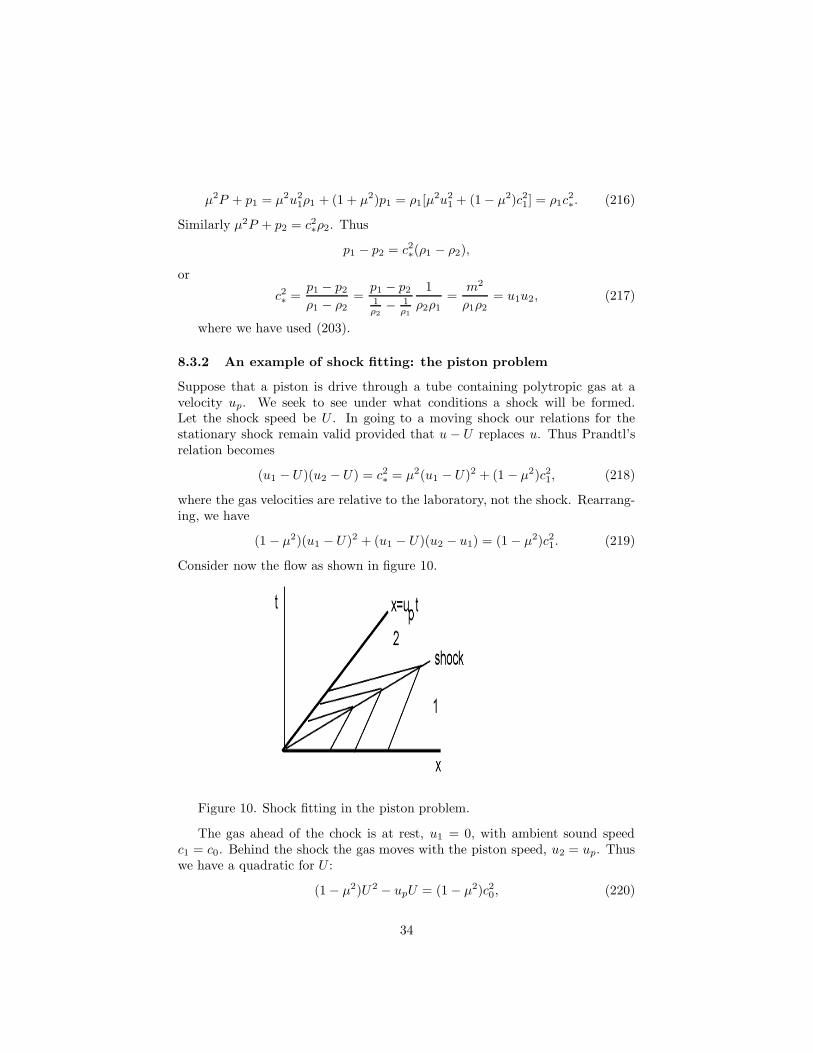
Consider now the flow as shown in figure 10.
Figure 10. Shock fitting in the piston problem.
The gas ahead of the chock is at rest, u1 = 0, with ambient sound speedc1 = c0. Behind the shock the gas moves with the piston speed, u2 = up. Thuswe have a quadratic for U :
(1 − µ2)U2 − upU = (1 − µ2)c20, (220)
34
giving
U =up + sqrtu2
p + 4(1 − µ2)c202(1 − µ2)
. (221)
We see that a shock forms for any piston speed. If up is small compared to c0,the shock speed is approximately c0, but slightly faster, as we expect. To getthe density ρp behind the shock in terms of that ρ0 of the ambient air, we notethat mass conservation gives (up − U )ρp = −Uρ0 or
ρp =U
U − upρ0. (222)
35