nonlinear trivelpiece-gould waves: frequency, functional...

Nonlinear Trivelpiece-Gould waves: Frequency, functional form, and stability

D. H. E. Dubin and A. AshourvanDepartment of Physics, UCSD, La Jolla, California 92093, USA

(Received 10 August 2015; accepted 14 September 2015; published online 6 October 2015)

This paper considers the frequency, spatial form, and stability of nonlinear Trivelpiece-Gould (TG)

waves on a cylindrical plasma column of length L and radius rp, treating both traveling waves and

standing waves, and focussing on the regime of experimental interest in which L=rp � 1. In this re-

gime, TG waves are weakly dispersive, allowing strong mode-coupling between Fourier harmon-

ics. The mode coupling implies that linear theory for such waves is a poor approximation even at

fairly small amplitude, and nonlinear theories that include a small number of harmonics, such as

three-wave parametric resonance theory, also fail to fully capture the stability properties of the sys-

tem. It is found that nonlinear standing waves suffer jumps in their functional form as their ampli-

tude is varied continuously. The jumps are caused by nonlinear resonances between the standing

wave and nearly linear waves whose frequencies and wave numbers are harmonics of the standing

wave. Also, the standing waves are found to be unstable to a multi-wave version of three-wave

parametric resonance, with an amplitude required for instability onset that is much larger than

expected from three wave theory. It is found that traveling waves are linearly stable for all ampli-

tudes that could be studied, in contradiction to three-wave theory. VC 2015 AIP Publishing LLC.

[http://dx.doi.org/10.1063/1.4932001]

I. INTRODUCTION

In this paper, we consider the theory of nonlinear

Trivelpiece-Gould (TG) waves on a cylindrical cold plasma

column. These plasma waves have been studied in theory

and in experiments spanning several decades of research,1–5

and their nonlinear behavior has recently received renewed

attention.6,7 Their linear dispersion relation is also similar to

that of cold magnetized plasma waves in a uniform plasma,

ion acoustic waves,8 and shallow water waves in the

Boussinesq approximation, the nonlinear behavior of which

has been extensively studied.9

Here, we construct nonlinear solutions for both traveling

and standing TG waves, focussing on the regime of current

experimental interest, L=rp � 1, where L and rp are the

plasma column length and radius, respectively. The traveling

waves are described using periodic boundary conditions, and

the standing waves are described with Neumann conditions

appropriate to the experiments. In the regime L=rp � 1,

these waves are only weakly dispersive. Consequently, these

TG waves display strong nonlinear effects even at small am-

plitude. For a system with weak dispersion, a harmonic of a

finite amplitude wave, with a frequency and wavenumber

that are a given multiple of the fundamental, is nearly on the

linear dispersion relation themselves and consequently is

driven resonantly to large amplitude by the fundamental,

through nonlinear mode coupling. This implies that linear

theory is a poor approximation for such waves, even at small

amplitudes, and also that nonlinear theories that incorporate

only a few harmonics, such as perturbation theory, or the

theory of three-wave parametric resonance, are of limited

usefulness.

The traveling-wave solutions that we construct display a

strong positive nonlinear frequency shift with increasing am-

plitude, up to a maximum amplitude associated with the

formation of a stagnation point in the fluid flow. Soliton sol-

utions are also found, with the usual K-dV functional form at

low amplitude10,11 and a more strongly peaked form at larger

amplitudes. For standing waves, we observe a novel behav-

ior: apparently discontinuous jumps in the functional form of

the standing wave solutions as amplitude is varied. The

jumps have the appearance of a nonlinear resonance, in

which a high-order Fourier mode in the solution becomes

excited, producing a ripple whose amplitude increases as the

resonance is approached, and then switches phase by 180�

across the resonance. In fact, each observed jump can be cor-

related to a degeneracy between the amplitude-dependent

nonlinear standing wave frequency and a nearly linear wave

that has given multiples of the standing wave frequency and

wavenumber. These waves are resonantly excited by the

standing wave because it contains many harmonics of the

fundamental in both space and time.

We then analyze the linear stability of these waves with

respect to small perturbations of the nonlinear waveform. An

oft-used model of instability is reviewed: three-wave para-

metric resonance, in which a nonlinear wave (termed the

pump wave in three wave theory) interacts with two longer-

wavelength “daughter waves.”12–15 When a resonance condi-

tion is met, the daughter waves can be driven unstable by the

pump wave. Such parametric resonances are observed in

many nonlinear systems, including TG waves. In fact, sev-

eral aspects of the observations of the nonlinear TG wave

instability can be fitted by the three-wave model.6

However, the actual system is not confined to only three

waves. Neither the nonlinear pump wave nor the growing

daughter waves are single Fourier modes, as is assumed in

three wave theory. Even at moderate amplitudes, mode-

coupling produces many Fourier harmonics in the nonlinear

waves, which have a strong effect on their stability,

1070-664X/2015/22(10)/102102/27/$30.00 VC 2015 AIP Publishing LLC22, 102102-1

PHYSICS OF PLASMAS 22, 102102 (2015)

This article is copyrighted as indicated in the article. Reuse of AIP content is subject to the terms at: http://scitation.aip.org/termsconditions. Downloaded to IP:

132.239.73.69 On: Tue, 06 Oct 2015 18:04:52

http://dx.doi.org/10.1063/1.4932001

http://dx.doi.org/10.1063/1.4932001

http://crossmark.crossref.org/dialog/?doi=10.1063/1.4932001&domain=pdf&date_stamp=2015-10-06

particularly for L=rp � 1. When the correct form of the

pump and daughter waves is used, keeping multiple Fourier

harmonics in each, we find that the system is far less unstable

than three wave theory would predict.

For nonlinear traveling waves, we find that the solutions

are stable for all amplitudes we could consider with the

Fourier method employed in this paper. For standing waves,

we find that there is a range of amplitudes which are unsta-

ble, depending on the parameters of the TG dispersion rela-

tion, in particular, the perpendicular wavenumber k?, a

parameter in the dispersion relation proportional to 1=rp.

However, the amplitude required for instability onset is

much larger than predicted by three-wave theory, particu-

larly for k?L� 1, and the calculated growth rate is smaller.

In Section II, we introduce the fluid equations used to

describe TG waves. In Section III, we analyze the functional

form and frequency of nonlinear traveling TG waves using

two methods: a direct integration of the differential equations

in Sec. III A, and a Fourier expansion of the solution in Sec.

III B. In Sec. III B 1, we analyze the form of the nonlinear

wave and the wave phase velocity in a small amplitude per-

turbation expansion. In Section IV, we analyze the functional

form of nonlinear standing waves using a Fourier expansion

and consider the small amplitude limit as a perturbation

expansion. In Section V A, we consider the linear stability of

traveling waves, and in Section V B we examine the stability

of standing waves, using both three wave theory and the

more general M-wave theory. Results and open questions are

discussed in Sec. VI. Appendix A contains a brief analysis of

the k? ¼ 0 limit of the equations, and Appendix B describes

the method employed in our nonlinear simulations of the TG

system.

II. MODEL

We consider nonlinear magnetized Langmuir

(Trivelpiece-Gould) waves in a cold but collisionless homo-

geneous plasma column with radius rp, length L, and uniform

equilibrium density n0. The plasma column is held inside a

conducting cylinder of radius rw by a strong uniform mag-

netic field in the z direction (along the axis of the column).

Neglecting cyclotron motion and cross-magnetic field drifts,

particles move only in the z direction in response to the elec-

trostatic field of the wave. We use cold fluid theory to

describe the plasma motion and concentrate on azimuthally

symmetric modes. The plasma density n, fluid velocity v,

and electrostatic potential / are then functions only of time

t, axial position z, and cylindrical radius r. The cold fluid

equations of motion for these three functions are

@n

@tþ @

@znvð Þ ¼ 0; (1)

@v

@tþ v

@v

@z¼ � @/

@z; (2)

1

r

@

@rr@/@r

� �þ @

2/@z2¼ �n; (3)

where for simplicity all quantities are dimensionless: density

is normalized to the (constant) equilibrium density n0,

distance is normalized by the fundamental axial wavenumber

of the plasma column k1 ¼ p=L, time is normalized to the

plasma frequencyffiffiffiffiffiffiffiffiffiffiffiffiffiffiffiffiffiffiffiffi4pe2n0=m

p, velocity is normalized to

xp=k1, and electrostatic potential to mx2p=ek2

1.

Equations (1)–(3) form a closed set, amenable to numer-

ical and analytical study. However, radial dependence and fi-

nite plasma length effects in the equations are complicating

factors. To simplify, we further assume that the plasma is a

long thin column and neglect end effects, taking periodic

boundary conditions with period 2L.16,17 We also simplify

by integrating over the radial dependence using the follow-

ing argument.3 We concentrate on nonlinear plasma modes

with no radial nodes (i.e., the lowest radial standing mode).

For these modes, low amplitude (linear) perturbations to the

equilibrium have a Bessel function radial dependence within

the plasma, described as

nðr; z; tÞ ¼ 1þ J0ðk?rÞdnðz; tÞ;vðr; z; tÞ ¼ J0ðk?rÞdvðz; tÞ;/ðr; z; tÞ ¼ /0ðrÞ þ J0ðk?rÞd/ðz; tÞ; (4)

where /0ðrÞ is the equilibrium plasma potential, k? is the

(scaled) perpendicular wavenumber, given by

k2? ¼

2

�r2p ln rw=rp

� � ; (5)

and �rp ¼ k1rp is the scaled plasma radius. Equation (5) is

valid provided that L=rw � 1. (A more general expression

for k? can be found in Ref. 18.) Approximate nonlinear

equations may then be obtained by substituting Eqs. (4) into

Eqs. (1)–(3) and integrating over radius out to rp. This sim-

plification neglects nonlinear mixing of different radial

modes.3 The result is a set of nonlinear equations

@N

@tþ @

@zNVð Þ ¼ 0; (6)

@V

@tþ V

@V

@z¼ � @U

@z; (7)

@2U@z2� k2

?U ¼ 1� N; (8)

where Nðz;tÞ¼1þbdnðz;tÞ;Vðz;tÞ¼bdvðz;tÞ;Uðz;tÞ¼bd/ðz;tÞ,and

b ¼ 2=�r2p

� �ð�rp

0

rdrJ0 k?rð Þ ¼ 2

k?�rpJ1 k?�rpð Þ

�1� k2?�r2

p=8; k?�rp < 1; (9)

is a scaling factor. (Somewhat different scaling factors can

be obtained depending on how one defines the radial aver-

age.) Equations (6)–(8) are identical to those found in Ref. 3

except that here we keep the second derivative in z of the

potential in the Poisson equation as it provides the (weak)

dispersion necessary for the existence of nonlinear periodic

solutions. For low (but not infinitesimal) amplitudes, these

equations have been previously shown to have soliton

102102-2 D. H. E. Dubin and A. Ashourvan Phys. Plasmas 22, 102102 (2015)


132.239.73.69 On: Tue, 06 Oct 2015 18:04:52

solutions identical to those of the K-dV equation.11 Similar

equations have also been studied in other contexts. For

example, if one replaces the Poisson equation (8) by

@2U@z2¼ exp Uð Þ � N; (10)

one has a model for nonlinear ion sound waves.20 If one

instead drops Eq. (8) and replaces Eq. (7) by

@V

@tþ V

@V

@z¼ �k�2

?@

@zN þ @

2N

@t2

� �; (11)

one obtains a well-known form of the Boussinesq equations

describing slightly dispersive nonlinear shallow water

waves.19 Both these models have the same linear dispersion

relation as Eqs. (6)–(8)

x2 ¼ m2=ðm2 þ k2?Þ; (12)

(with k? ¼ 1 in the ion sound wave model), where perturba-

tions for linear mode m have (unscaled) axial wavenumber

km ¼ mk1.

The k? ¼ 0 form of Eqs. (6)–(8) describes unmagne-

tized Langmuir waves in a cold 1D plasma. This well-

studied system21 admits a general nonlinear analytic solution

in Lagrangian coordinates. It is highly degenerate, with all

initial perturbations oscillating at the plasma frequency (as

seen in a frame where the mean plasma velocity is zero), in-

dependent of spatial form or amplitude, provided that the

amplitude is sufficiently small so that characteristics do not

cross. This case is discussed briefly in Appendix A. The fi-

nite temperature extension of this system has also been

closely studied, as it exhibits a self-focussing instability

termed “Langmuir collapse.”22

Here, we focus on the zero-temperature k? > 1 regime of

interest in experiments on TG waves. We construct fully non-

linear traveling and standing wave solutions to Eqs. (6)–(8).

We then study the stability of these solutions, focusing on

instability due to 3-wave parametric resonance. It is necessary

to go beyond the small-amplitude K-dV version of the equa-

tions in order to study parametric instability, because we will

see that onset of the instability only occurs (when it occurs at

all) for large amplitudes with N � 1 � Oð1Þ.

III. TRAVELING WAVE SOLUTIONS

In this section, we construct nonlinear traveling-wave

solutions of our model equations (6)–(8) using two methods.

Both methods use the standard traveling-wave ansatz

whereby functions of t and z are assumed to depend only on

the combination z� ut � s, where u is the velocity of the

nonlinear wave. In what follows, we assume that u> 0 (the

traveling wave moves to the right). This ansatz reduces Eqs.

(6)–(8) to coupled ordinary differential equations that can be

solved using standard techniques

�u@N

@sþ @

@sNVð Þ ¼ 0; (13)

�u@V

@sþ V

@V

@s¼ � @U

@s; (14)

@2U@s2� k2

?U ¼ 1� N: (15)

In method 1, we directly integrate the equations. In method

2, we solve them via Fourier methods.

A. Method 1: Direct integration

In this method, it is useful to scale Eqs. (13)–(15) one

more time, so as to remove the dependence on the parameter

k?. Define �u ¼ u=k?; �v ¼ V=k?; �s ¼ k?s; and �U ¼ k2?U.

Then, in these rescaled variables, Eqs. (13)–(15) become

��u@N

@�sþ @

@�sN�vð Þ ¼ 0; (16)

��u@�v

@�sþ �v

@�v

@�s¼ � @

�U@�s

; (17)

@2 �U@�s2� �U ¼ 1� N: (18)

[Effectively, this rescaling replaces the factor k1 by k? in the

original scalings discussed after Eq. (3).] Direct integration

of Eq. (16) then implies that

Nð�sÞ ¼ C=½�u � �vð�sÞ�; (19)

where C is a constant of integration, related to the particle

flux as seen in the moving frame. Equation (19) implies that

�vðsÞ < �u is necessary, otherwise there is a stagnation point

where the density approaches infinity. Integration of Eq. (17)

implies an energy conservation relation

1

2�u � �v �sð Þð Þ2 þ �U �sð Þ ¼ E; (20)

which implies

�u � �vðsÞ ¼ffiffiffiffiffiffiffiffiffiffiffiffiffiffiffiffiffiffiffiffiffiffiffiffiffi2ðE� �UðsÞÞ

q: (21)

In order to avoid singularities, Eq. (21) implies that

�Uð�sÞ E; (22)

is required. Application of Eqs. (21) and (19) to Eq. (18)

then yields

@2 �U@�s2¼ � @V

@ �U; (23)

where the potential function Vð�UÞ is

V �Uð Þ ¼ ��U � 1

2�U

2 � Cffiffiffiffiffiffiffiffiffiffiffiffiffiffiffiffiffiffiffi2 E� �Uð Þ

p: (24)

There are a range of C and E values for which Vð�UÞ forms a

potential well in which oscillatory solutions for �Uð�sÞ can be

obtained from Eq. (23). A typical case is displayed in Fig. 1.

There is a local minimum at �Ub and a local maximum at �Ua.



132.239.73.69 On: Tue, 06 Oct 2015 18:04:52

Oscillations in �U occur between a minimum amplitude �Umin

and a maximum amplitude �Umax, with �Ua �Umin �Ub and�Umax E required.

The range of possible values of C and E for which oscil-

latory solutions occur is shown in Fig. 2. The upper limit on

C is given by the curve C ¼ffiffiffiffiffiffi2Ep

. On this curve, one of the

two local extrema in V occurs at �U ¼ 0. When E< 1=2, this

extremum is a local minimum, allowing small oscillations of�U around zero (i.e., linear waves). On the other hand, when

E> 1=2 the extremum is a local maximum producing a soli-

ton solution as discussed below. That is, solitons occur for

1=2 E 2 and C ¼ffiffiffiffiffiffi2Ep

, and linear waves occur along

the same curve C ¼ffiffiffiffiffiffi2Ep

but with 0 E < 1=2. Linear

waves and solitons are analyzed in more detail below.

The minimum limit on possible C values for given Eshown in Fig. 2 corresponds to waves with the maximum

possible amplitude, �Umax ¼ E (see Eq. (22)). At this ampli-

tude, there are stagnation points in the fluid where the

density approaches infinity. The minimum and maximum

curves meet at C ¼ E ¼ 2, which corresponds to a soliton

with a stagnation point. The curves also meet at C ¼ E ¼ 0,

where solutions become singular with wave numbers

approaching infinity and amplitudes approaching zero;

depending on how the limits C! 0 and E! 0 are taken the

waves range from linear to highly nonlinear.

From the form of the equation of motion, Eq. (23), there

is an energy invariant H associated with the oscillation,

given by

H ¼ 1

2

d �Ud�s

� �2

þV �Uð Þ; (25)

where H ¼Vð�UminÞ ¼Vð�UmaxÞ (see Fig. 1). Note that Hand �Umin are both determined by �Umax. We will therefore

parameterize our nonlinear solutions by �Umax; the maximum

value of the potential during the oscillation.

These oscillatory solutions must satisfy certain constraints.

Let us denote the wavelength of the oscillation as �k [i.e., the

oscillatory solution obeys �Uð�s þ �kÞ ¼ �Uð�sÞ] and define an av-

erage over a period of oscillation as hi ¼ 1�k

Ð �sþ�k�s d�s. Then, we

require the solutions to obey the constraint

hNi ¼ 1; (26)

i.e., mean density is unchanged from the equilibrium value.

Taking an average of Eq. (20), using Eq. (26) and the iden-

tity hd2 �U=d�s2i ¼ 0 then implies that our solutions must obey

h�Ui ¼ 0: (27)

In addition to these constraints, we require that the mean

flow velocity vanishes

hN�vi ¼ 0: (28)

This equation defines the lab frame of reference. In other

words, the velocity of the wave, �u, is measured with respect

to the frame in which the mean fluid velocity vanishes. In

this frame, fluid elements oscillate in the wave but there is

no net translation of the fluid.

An expression for the phase velocity can then be found

by multiplying both sides of Eq. (19) by �u � �v and taking the

mean

hN�ui � hN�vi ¼ �u ¼ C; (29)

where on the left hand side we applied Eqs. (26) and (28).

Now, Eq. (25) can be used to obtain an expression for

the wavelength �k. This equation implies that

ds ¼ d �U=ffiffiffiffiffiffiffiffiffiffiffiffiffiffiffiffiffiffiffiffiffiffiffiffiffiffiffi2½H �Vð�UÞ�

q: (30)

Integrating both sides over a half-period of the oscillation,

during which �U varies from �Umin to �Umax, implies that

�k ¼ 2

ð�Umax

�Umin

d �Uffiffiffiffiffiffiffiffiffiffiffiffiffiffiffiffiffiffiffiffiffiffiffiffiffiffiffiffiffiffiffiffiffiffiffiffiffiffiffiffiffiffiffi2 V �Umaxð Þ �V �Uð Þ� �q ; (31)

FIG. 1. The potential function Vð�UÞ.

FIG. 2. The shaded area is the region in the E versus C plane for which non-

linear traveling-wave solutions occur. The red, black, and green dotted

curves are contours of constant wavenumber �k with values 1, 1/3, and zero,

respectively. The zero-wavenumber solutions are solitons. Along each con-

tour, the amplitude increases as one moves from left to right, from linear

waves on the left to waves with stagnation points on the right.



132.239.73.69 On: Tue, 06 Oct 2015 18:04:52

where we have used H ¼Vð�UmaxÞ. This shows that�k ¼ �kðE;C; �UmaxÞ. (The dependences on C and E arise

through the dependence of V on these variables; see Eq.

(24); and we again note that �Umin depends on �Umax through

the relation Vð�UminÞ ¼Vð�UmaxÞ.) However, Eq. (27)

implies a relation between C, E, and �Umaxð�k

0

d�s �Uð�sÞ ¼ 0:

Assuming that �s ¼ 0 corresponds to �U ¼ �Umax, we convert

the integration over �s to one over �U using Eq. (30), to obtain

ð �Umax

�Umin

d �U �Uffiffiffiffiffiffiffiffiffiffiffiffiffiffiffiffiffiffiffiffiffiffiffiffiffiffiffiffiffiffiffiffiffiffiffiffiffiffiffiffiffiffiffi2 V �Umaxð Þ �V �Uð Þ� �q ¼ 0: (32)

For given values of E and �Umax, Eq. (32) can be solved

for C to obtain C ¼ CðE; �UmaxÞ. This, together with Eq. (31),

allows us to determine the wavelength �k as a function of Eand �Umax. Thus, for given mode amplitude �Umax, the wave-

length may be varied by changing E. In Fig. 3, we plot the

range of possible wave numbers �kðE; �UmaxÞ ¼ 2p=�kðE; �UmaxÞfor given amplitude �Umax. There is a maximum possible wave-

number for a given mode amplitude �Umax, corresponding to

the case where E ¼ �Umax, which results in the aforementioned

stagnation points where �vð�sÞ ¼ �u and Nð�sÞ ! 1 at the values

of �s where �U ¼ �Umax ¼ E. The figure shows that for infinites-

imal amplitude (linear waves) all wave numbers are allowed,

but as �Umax approaches the maximum possible value of 2, the

only allowed wavenumber is zero (i.e., a soliton with a stagna-

tion point). Soliton solutions with lower amplitudes corre-

spond to �k ¼ 0 in this figure. For the periodic boundary

conditions of interest in this paper, only certain discrete values

of �k are allowed, given by �k ¼ m=k? for integer m.

Finally, the nonlinear wave phase velocity follows from

the wave speed equation (29):

�uðE; �UmaxÞ ¼ CðE; �UmaxÞ: (33)

We can invert �k ¼ �kðE; �UmaxÞ to obtain E ¼ Eð�k; �UmaxÞ and

use this to write �u ¼ CðEð�k; �UmaxÞ; �UmaxÞ, i.e., wave phase

velocity versus wavenumber and amplitude. This is plotted

in Fig. 4 for four different amplitudes. The dashed line is for

amplitude approaching zero

�uð�k; �Umax ¼ 0Þ ¼ 1=

ffiffiffiffiffiffiffiffiffiffiffiffiffi1þ �k

2

q; (34)

which corresponds to the phase velocity given by the linear

dispersion relation (12) in barred units where �k ¼ m=k? and

�u ¼ k?u.

Fig. 5 displays the potential, density, and velocity versus

position �s for waves with �k ¼ 1=3 and for several different

amplitudes, and Fig. 6 displays the potential for waves with�k ¼ 0 (i.e., solitons). The potential was determined by first

finding the values of E and C corresponding to �k ¼ 1=3 and

the given values of �Umax, and then solving Eq. (23) numeri-

cally for these values. For small amplitude, the waves are

nearly sinusoidal, but as the amplitude grows the waves

become more sharply peaked until at the maximum possible

amplitude the stagnation point produces a cusp in the poten-

tial and velocity functions, and a singularity in the density.

Comparing Figs. 5 and 6, one can see that at larger ampli-

tudes the soliton solutions are qualitatively similar to the fi-

nite �k solutions.

1. Linear waves and solitons

Small amplitude waves can be analyzed by Taylor-

expansion of the potential function Vð�UÞ, Eq. (24), in small�U

V �Uð Þ ’ �ffiffiffiffiffiffi2Ep

Cþ Cffiffiffiffiffiffi2Ep � 1

� ��U

þ 1

2

C

2Eð Þ3=2� 1

!�U

2 þ C

2 2Eð Þ5=2�U

3 þ (35)

For linear waves, it is sufficient to keep only up to the quad-

ratic terms in �U, which provide a harmonic well for the

potential oscillations. Such oscillations must satisfy Eq. (27),

and therefore the coefficient of the linear term in �U in Eq.

(35) must vanish, which implies C ¼ffiffiffiffiffiffi2Ep

for linear waves.FIG. 3. The shaded area gives the region of allowed wavenumber �k versus

mode amplitude �Umax.

FIG. 4. The phase velocity �u of traveling waves versus wavenumber �kfor four different amplitudes, �Umax ¼ 0 (the dashed line), as well as�Umax ¼ 0:1; 0:5; and 1, in order of increasing magnitude of �u in the plot.

The solid black line is the outer envelope of allowed velocities and

wavenumbers.



132.239.73.69 On: Tue, 06 Oct 2015 18:04:52

When this relation is employed in Eq. (35), the coefficient of

the quadratic term in �U provides the frequency (actually, the

wavenumber �k since �s is a position) of harmonic oscillations

in the potential

�k2 ¼ 1

2E� 1

� �: (36)

Since the square of the wavenumber should be positive-

definite for oscillatory solutions, this implies that E< 1=2 is

required for linear waves, as discussed previously in relation

to Fig. 2. The linear dispersion relation then follows from

Eq. (29), which implies �u ¼ffiffiffiffiffiffi2Ep

. Applying this relation to

Eq. (36) yields �k2 ¼ 1=�u2 � 1, which can be rearranged to

produce the linear dispersion relation, Eq. (34).

Solitons occur when �Umin coincides with the local maxi-

mum �Ua, so that the period of oscillation in the potential well

Vð�UÞ approaches infinity (see Fig. 1). However, the require-

ment that h�Ui ¼ 0 then implies that �Umin ¼ �Ua ¼ 0. From

Eq. (35), the local maximum �Ua equals zero when C ¼ffiffiffiffiffiffi2Ep

and E> 1=2. This is the dotted green curve in Fig. 2.

The soliton amplitude �Umax is related to E by the poten-

tial function Vð�UÞ. Since Vð�UmaxÞ ¼Vð�UminÞ, using Eq.

(24) for Vð�UÞ; C ¼ffiffiffiffiffiffi2Ep

, and �Umin¼ 0 then implies

��Umax �1

2�U

2

max � 2Effiffiffiffiffiffiffiffiffiffiffiffiffiffiffiffiffiffiffiffiffiffiffiffi1� �Umax=E

q¼ �2E: (37)

This equation can be solved for �Umax, yielding

�Umax ¼ 2ðffiffiffiffiffiffi2Ep

� 1Þ: (38)

Since the soliton amplitude must satisfy Eq. (22), when com-

bined with Eq. (38) this implies 1=2 E 2 for soliton sol-

utions, as shown in Fig. 2.

The soliton velocity versus amplitude follows from Eqs.

(29), (38), and the relation C ¼ffiffiffiffiffiffi2Ep

. From Eq. (29), this last

relation implies �u ¼ffiffiffiffiffiffi2Ep

. Combining this with Eq. (38) and

rearranging yields

�u ¼ 1þ 1

2�Umax: (39)

Thus, the maximum possible soliton velocity �u ¼ 2 occurs at

the maximum amplitude �Umax ¼ 2, as shown in Fig. 4. Also,

the maximum fluid velocity in the frame of the soliton is

�vð0Þ ¼ �Umax. This follows from Eqs. (21), (38), and (39).

The functional form of solitons, �Uð�sÞ, can be found by

integrating both sides of Eq. (30) to obtain �sð�UÞ, and then

inverting this expression. In general, the solitons can be

expressed in terms of elliptic integrals but the form is too com-

plex to merit reproduction here. Alternatively, they can be

found by numerically integrating the equation of motion, Eq.

(23). Solitons are shown in Fig. 6 for a range of amplitudes.

The functional form simplifies in two cases. For small ampli-

tudes, the solitons become K-dV solitons with functional form

�U �sð Þ ¼�Umax

cosh2 �sffiffiffiffiffiffiffiffiffiffi�Umax

p=2

� � : (40)

For the maximum amplitude �Umax ¼ 2, the soliton has a

stagnation point and can be expressed as the solution to the

following equation:

FIG. 5. Plots of the wave potential (a), fluid velocity (b), and density (c) for traveling waves over one wavelength �k, all with �k ¼ 1=3 (i.e., �k ¼ 6p), and with 5

different wave amplitudes: �Umax ! 0 (the dashed line), and in order of increasing narrowness, �Umax ¼ 0:1; 0:5; 1, and the maximum possible value at �k ¼1=3; �Umax ¼ 1:34 (see Fig. 3).

FIG. 6. (a) Wave potential versus position in solitons for three amplitudes: �Umax ! 0, (dashed), �Umax ¼ 1, (solid), and �Umax ¼ 2 (dotted). The potential is

scaled to �Umax and distance is scaled byffiffiffiffiffiffiffiffiffiffi�Umax

pso that the infinitesimal amplitude soliton, Eq. (40), is visible in the plot. (b) and (c) Fluid velocity and density

versus position in solitons, for the same amplitudes as in (a) as well as amplitude �Umax ¼ 0:1 (the dotted-dashed curve).



132.239.73.69 On: Tue, 06 Oct 2015 18:04:52

j�sj ¼ �2 ln 2� y�ffiffiffiffiffiffiffiffiffiffiffiffiffiffiffiffiffiffiffiffiffiffiffiffiffiffiffiffiffi1� yð Þ 3� yð Þ

ph i

þ 2ffiffiffi3p ln

3� 2y�ffiffiffiffiffiffiffiffiffiffiffiffiffiffiffiffiffiffiffiffiffiffiffiffiffiffiffiffiffiffiffi3 1� yð Þ 3� yð Þ

py

" #; (41)

where �U ¼ 2yð1� yÞ.

B. Method 2: Fourier expansion

In this subsection, we apply Fourier methods to deter-

mine the same nonlinear traveling-wave solutions as were

discussed in Sec. III A. The Fourier expansion method has

several advantages. First, the periodic boundary conditions

used in this paper are built directly into the method: the

wavenumber k discussed in Sec. III A is no-longer a continu-

ous variable but instead is automatically quantized to the

correct values for a given plasma length. Second, we will see

later that the method can also be applied to nonlinear stand-

ing wave solutions. Third, the Fourier method can be

extended in a natural way to allow determination of the sta-

bility of traveling and standing wave solutions. Finally, some

analytic results for low amplitude traveling waves can be

readily obtained using Fourier expansion, because at low

amplitudes the waves approach single Fourier modes.

In the Fourier approach, the traveling wave is expanded

as a sum of spatial Fourier modes, each with fundamental pe-

riod L. In the scaled units of Sec. III A, this period is 2p, and

the Fourier expansions take the following form:

NðsÞ ¼X1

m¼�1Nmeims; (42)

VðsÞ ¼X1

m¼�1Vmeims; (43)

UðsÞ ¼X1

m¼�1Umeims: (44)

Also, Eqs. (26) and (28) imply that the m¼ 0 Fourier coeffi-

cients must satisfy N0 ¼ 1 and U0 ¼ 0.

In this section, we choose to work in a moving frame,

one where hVi ¼ 0, rather than the frame implied by Eq.

(27). In this new frame, we call the phase velocity u0. It dif-

fers from u by the value of hNVi as seen in the new frame

u ¼ u0 � hNVi

¼ u0 �X1

m¼�1NmV�m: (45)

We make this frame change because the condition hVi ¼ 0

is simple to implement in the Fourier method, requiring only

that we set Fourier mode V0 ¼ 0. Once we have obtained the

solution in the moving frame, we can use Eq. (45) to deter-

mine u in the lab frame.

First, we use Eqs. (42) and (44) in Eq. (8) to obtain the

following relation between density and potential:

Um ¼Nm

m2 þ k2?: (46)

Next, substituting these expansions into Eqs. (6) and (7)

and taking the mth Fourier harmonic (m 6¼ 0) of the resulting

equations imply

�u0mNm þ mX1

l¼�1VlNm�l ¼ 0; (47)

�u0mVm þX1

l¼�1lVlVm�l ¼ �amNm; (48)

where

am � m=ðm2 þ k2?Þ: (49)

Equations (47) and (48) constitute a nonlinear eigen-

value problem for the m 6¼ 0 Fourier coefficients Nm and vm,

where the eigenvalue is the phase velocity u0. There is

always a trivial solution to these equations, Nm ¼ vm ¼ 0;

but for special values of u0 there are nontrivial solutions cor-

responding to nonlinear traveling waves.

Symmetry in these equations allows us to specify, with-

out loss of generality, that all the Fourier coefficients are real

and satisfy N�m ¼ Nm and v�m ¼ vm, so that the traveling-

wave solutions are even in s. Thus, we need only consider

the m> 0 Fourier coefficients as independent variables in the

equations.

Due to spatial homogeneity of the system, any eigen-

mode with period 2p and a given value of the perpendicular

wavenumber k? can be mapped, by rescaling distances, into

an infinite set of other eigenmodes with period 2p=l for inte-

ger l greater than one, each eigenmode with perpendicular

wavenumber lk?, and wave velocity u0=l. Therefore, we con-

sider only the lowest-order eigenmode with period 2p, over a

range of k? values, and a range of amplitudes. For small

amplitudes, this eigenmode is concentrated in the m¼ 1

Fourier harmonic.

In order to find these nontrivial solutions, we first ap-

proximate the equations by keeping only a finite number of

Fourier modes, allowing m to range only over �M m Mfor integer M> 0, and setting all Fourier coefficients outside

this range equal to zero. Equations (47) and (48) then involve

2M independent equations in the 2M independent unknowns

Nm and vm, 1 m M (the m< 0 equations and unknowns

are not independent).

We next parametrize the wave amplitude by the first

Fourier coefficient of the density, N1, i.e., we set this coeffi-

cient equal to a given amplitude value A, a real number

greater than or equal to zero. This removes one of the

unknown variables from the set of equations and makes the

equations inhomogeneous. However, noting that u0 is also an

unknown quantity, we can now solve the 2M inhomogeneous

nonlinear equations for u0 along with the 2M � 1 unknown

Fourier coefficients. Since the equations are now inhomoge-

neous their solution is fairly straightforward, parametrized

by the values of A and k?. For small amplitudes, the solution

can be obtained using perturbation theory, and for larger

amplitudes we use Newton’s method. The solutions match

those found in Sec. III A provided that a sufficiently large

value of M is used. This becomes problematic for waves



132.239.73.69 On: Tue, 06 Oct 2015 18:04:52

with stagnation points, where the density exhibits a singular-

ity and its Fourier expansion converges slowly; or for soli-

tons, which are not periodic; but for moderate amplitudes

and finite wavelengths the Fourier method works well.

In Fig. 7, the wave phase velocity u is plotted versus am-

plitude A for two values of k?. The phase velocity was

obtained using the Fourier approach by numerically solving

Eqs. (47) and (48) via Newtons method as described above,

keeping M¼ 40 Fourier modes. Once u0 was found from this

solution, Eq. (45) was applied to determine u. The phase veloc-

ity is compared to perturbation expansions obtained below. As

expected from Sec. III A, the phase velocity increases with

increasing wave amplitude. Note that k? ¼ 3 and k? ¼ 5 cor-

respond to �k ¼ 1=3 and �k ¼ 1=5, respectively, in Fig. 4. In

Fig. 8, we plot the maximum wave potential Umax ¼ Uðs ¼ 0Þand maximum density Nmax ¼ Nðs ¼ 0Þ versus the Fourier

amplitude coefficient A for different values of k?. At low

amplitudes, the maximum density is Nmax ¼ 1þ 2A and the

maximum potential is Umax ¼ 2A=ð1þ k2?Þ. [In order to com-

pare Figs. 7 and 8 to results in Sec. III A, recall that �U ¼ k2?U

and �u ¼ k?u.]

Figures 7 and 8 show that as k? increases, waves are

more nonlinear for a given amplitude (i.e., they depart more

from linear theory). This is because larger k? implies less lin-

ear dispersion, and it is dispersion that acts against the steep-

ening effect of nonlinearity in these waves. Ultimately, in the

limit of no dispersion (i.e., k? ! 1), even infinitesimal

amplitude waves will exhibit nonlinear steepening and wave-

breaking, in the absence of mitigating effects not included in

our theory, such as viscosity.

1. Small amplitude perturbation expansion

For small amplitudes, A� 1, a perturbative solution of

Eqs. (47) and (48) can be found by expanding the variables

in powers of A. We assume that Nm ¼ 0ðAmÞ for m> 1, and

similarly for vm. In detail, we substitute the following pertur-

bative expansions into Eqs. (46)–(48):

Nm ¼ AmX1n¼0

A2nNm;2n;m > 1; (50)

Vm ¼ AmX1n¼0

A2nvm;2n;m > 0; (51)

u0 ¼X1n¼0

A2nu2n: (52)

We then collect powers of A and solve the equations at each

order of A in the unknown expansion coefficients appearing

at that order, assuming that N1 ¼ A.

At first order in A, Eqs. (47) and (48) are nontrivial only

for m¼ 1, becoming the linearized equations

�u0Aþ Av1;0 ¼ 0; (53)

�Au0v1;0 ¼ �a1A: (54)

Solving Eqs. (53) and (54) for v1;0 and u0 yields the lin-

ear dispersion relation (see Eq. (34) for m¼ 1) as well as the

linear fluid velocity coefficient

u20 ¼ a1; (55)

v1;0 ¼ u0: (56)

At second order in A, nontrivial terms appear only in the

m¼ 2 equations, which become, after using Eqs. (55) and

(56)

2ð�u0N2;0 þ v2;0 þ u0Þ ¼ 0; (57)

a2N2;0 � 2u0v2;0 þ a1 ¼ 0: (58)

When solved for N2;0 and v2;0, these equations yield

FIG. 7. The phase velocity u of traveling waves versus Fourier amplitude Afor two transverse wave numbers, k? ¼ 3 and k? ¼ 5. Dots: numerical solu-

tion of Eqs. (47) and (48). Solid lines: Eq. (68). Dashed lines: the same

expression, neglecting the A4 term.

FIG. 8. (a) Maximum traveling-wave

potential versus Fourier amplitude Afor two transverse wave numbers. (b)

Maximum density versus Fourier am-

plitude A for the same two transverse

wave numbers.



132.239.73.69 On: Tue, 06 Oct 2015 18:04:52

N2;0 ¼3a1

2a1 � a2

; (59)

v2;0 ¼ u0

a1 þ a2

2a1 � a2

: (60)

At third order in A, Eqs. (47) and (48) are nontrivial for

m¼ 1 and m¼ 3. The m¼ 1 equations involve v1;2 and u2

ð2a1 � a2Þðv1;2 � u2Þ þ u0ð4a1 þ a2Þ ¼ 0; (61)

ð2a1 � a2Þðv1;2 þ u2Þ � u0ða1 þ a2Þ ¼ 0: (62)

Solution of these equations yields the lowest-order nonlinear

correction to the wave phase velocity

u2 ¼ u0

5a1 þ 2a2

2 2a1 � a2ð Þ ; (63)

as well as the fluid velocity Fourier coefficient

v1;2 ¼ �u0

3a1

2 2a1 � a2ð Þ : (64)

Working to higher order, the next correction to the wave

phase velocity is found to be

u4 ¼3u0

8

18a41 þ 9a2

1a2 12a2 � 5a3ð Þ þ 4a32a3 þ 12a1a2

2 3a2 þ a3ð Þ � a31 45a2 þ 206a3ð Þ

2a1 � a2ð Þ3 3a1 � a3ð Þ: (65)

Using Eqs. (49), (63), and (65) in Eq. (52), the perturba-

tion expansion for the wave phase velocity can be expressed

as

u0=u0 ¼ 1þ A2

48þ 3k2

?� �

þ A4

64128þ 208k2

? þ 65k4? þ 3k6

?� �

þ 0 A6ð Þ: (66)

However, u0 is the phase velocity in a moving frame

where hVi ¼ 0. In the lab frame where hNVi ¼ 0, the veloc-

ity u is related to u0 by Eq. (45). In the moving frame, the

value of hNVi can be found using the Fourier coefficients

determined in the previous analysis (see Eq. (45)). To low-

est order, hNVi ¼ 2A2v1;0 ¼ 2A2u0. To next order, we find

that

hNViu0

¼ 2A2 þ 9A4a1a2

2a1 � a2ð Þ2þ 0 A6ð Þ

¼ 2A2 þ A4

21þ k2

?� �

4þ k2?

� �þ 0 A6ð Þ: (67)

Subtracting Eq. (67) from Eq. (66) yields the wave phase ve-

locity in the lab frame

u=u0 ¼ 1þ 3A2

4k2? þ

3A4

64k2? 16þ 11k2

? þ k4?

� �þ 0 A6ð Þ:

(68)

This expansion is compared to the numerical solution of Eqs

(47), (48), and (45) in Fig. 7, showing good agreement for

low to moderate wave amplitudes.

Note that as k? approaches zero, u approaches u0, inde-

pendent of wave amplitude. This is as expected from the

general arguments given in Appendix A. Cold Langmuir

waves with k? ¼ 0 have an amplitude-independent fre-

quency, and therefore their phase velocity is also independ-

ent of amplitude.

IV. STANDING WAVE SOLUTIONS

We now obtain standing wave solutions to Eqs. (6)–(8).

For a long, thin plasma column, it has been shown that stand-

ing TG waves satisfy approximate Neumann boundary condi-

tions on the potential: dU=dzðz ¼ 0Þ ¼ dU=dzðz ¼ pÞ ¼ 0.16

A Fourier expansion of the variables consistent with these

boundary conditions is

Nðz; tÞ ¼X1m¼0

NmðtÞ cos mz; (69)

Uðz; tÞ ¼X1m¼1

UmðtÞ cos mz; (70)

Vðz; tÞ ¼X1m¼1

VmðtÞ sin mz; (71)

where N0ðtÞ ¼ 1, and where Eq. (8) implies

Um tð Þ ¼ Nm tð Þm2 þ k2

?: (72)

These expansions are substituted into Eq. (6), and the cos mzcoefficient of the result is taken, yielding

_Nm tð Þ þ m

2

X1m0¼1

Vm0 Nm�m0 þ Nm0�m � Nmþm0½ � ¼ 0: (73)

Here, note that Nm¼ 0 for m< 0, which can be used to

change the limits in the sum over m0 for the first two terms in

the square bracket. Also, note that the m¼ 0 version of Eq.

(73) is trivially satisfied by N0 ¼ 1 and will therefore not be

used in the following arguments.

Similarly, the sin mz coefficient of Eq. (7) is

_Vm tð Þ þ 1

2

X1m0¼1

m0Vm0 Vm�m0 � Vm0�m þ Vmþm0½ � ¼ amNm:

(74)

Here as well, note that VmðtÞ ¼ 0 for m 0.



132.239.73.69 On: Tue, 06 Oct 2015 18:04:52

We are concerned here with standing wave solutions

that are periodic in time, so NmðtÞ and VmðtÞ each have sub-

sidiary Fourier series expansions in time

NmðtÞ ¼X1n¼0

Nm;n cos nxt; (75)

VmðtÞ ¼X1n¼1

vm;n sin nxt; (76)

where the frequency x is an unknown variable. When these

expansions are substituted into Eq. (73) and the sin nxt coef-

ficient is taken, the result is

�nxNm;n þm

4

X1m0¼1

X1n0¼1

vm0;n0 ½Nm�m0;n�n0 þ Nm0�m;n�n0

� Nm0þm;n�n0 þNm�m0;n0�n þ Nm0�m;n0�n � Nm0þm;n0�n

�Nm�m0;n0þn þ Nm0�m;n0þn � Nm0þm;n0þn� ¼ 0: (77)

Similarly, when the cos nxt coefficient of Eq. (74) is

taken, the result is

nxvm;n þ1

4

X1m0¼1

X1n0¼1

m0vm0;n0 ½�vm�m0;n�n0 þ vm0�m;n�n0

� vm0þm;n�n0 þ vm�m0;n0�n � vm0�m;n0�n þ vm0þm;n0�n

þ vm�m0;n0þn� vm0�m;n0þnþ vm0þm;n0þnð Þ 1� dn;0ð Þ�¼ amNm;n;

(78)

where dn;0 is a Kronecker delta function. Equation (77) is

valid for m � 1 and n � 1, while Eq. (78) is valid for m � 1

and n � 0.

Equations (77) and (78) are a nonlinear eigenvalue prob-

lem for standing waves, similar to Eqs. (47) and (48) for

traveling waves. The equations can be solved using the same

method as for Eqs. (47) and (48). First, the system is made fi-

nite by imposing a maximum wavenumber and frequency.

We take m M and n M, and set the Fourier coefficients

Nm;n and vm;n to zero beyond these ranges. Next, we take

N1;1 ¼ A where A is a given real number greater than zero,

the amplitude of the nonlinear wave. This picks out the

eigenfunction with the lowest fundamental wavenumber,

m¼ 1. (If instead we had taken N1;1 ¼ 0 and N2;1 ¼ A, we

would have picked out an eigenfunction with fundamental

wavenumber m¼ 2.) We then solve the equations for the

other Fourier coefficients along with the mode frequency x.

The solution can be found either numerically via Newton’s

method or as a perturbation expansion in A, as was done for

traveling waves. A symmetry of the equations implies that if

m is even then only even n terms are nonzero, and if m is

odd, only odd n terms are nonzero. This reduces the number

of variables and equations to M2 þM=2 (assuming M is

even). Nevertheless, this problem is more difficult than the

traveling-wave problem where the number of unknowns and

equations scaled linearly with M, because there was no time

dependence in the traveling-wave solution when viewed in

the wave frame.

We have solved Eqs. (77) and (78) for a range of ampli-

tudes A and for several k? values. In order to obtain con-

verged solutions at the largest amplitudes, an M value of up

to 60 was employed, requiring the numerical solution of

3630 coupled nonlinear equations using Newton’s method.

The frequency of the waves is displayed in Fig. 9 versus am-

plitude A for four values of k?, and compared to perturbation

expansions valid for small A, derived below. As amplitude

increases, the wave frequency increases in a manner similar

to the traveling wave case discussed previously.

The harmonic content of the waves increases as the am-

plitude of the wave increases. In Fig. 10, we display the

Fourier coefficients Nmm versus amplitude, for k? ¼ 5. As Aincreases each coefficient increases roughly as Nm;m � Am.

This is the scaling expected in perturbation theory, as we

will show in Sec. IV A.

The spatial form of the density is displayed in Fig. 11 at

an instant of maximum amplitude, which occurs twice per

period, for instance, at t¼ 0 and at t ¼ p=x. At time t¼ 0,

the density peak is at one end of the column, z¼ 0, and at

t ¼ p=x the peak has shifted to the other end of the column,

at z ¼ p (z¼L in unscaled units) (the instant shown in the

figure, which displays 0 < z < 2L in unscaled units). At

these times, the fluid velocity is zero. The spatial form at t ¼p=x is identical to the form at t¼ 0, except for an overall

FIG. 9. Frequency versus amplitude A in nonlinear standing waves, normal-

ized to the linear frequency x0, for four values of k?. Points: frequency

obtained from numerical solution of Eqs. (77) and (78). Dashed line: the

lowest-order (A2) correction to the frequency. Solid line: frequency includ-

ing the A4 correction. Both corrections are included in Eq. (101).

FIG. 10. Fourier coefficients Nm;m in a nonlinear standing wave with

k? ¼ 5, versus wave amplitude A. The lines are aids to the eye of the form

Am for m ¼ 2; 3; 4; 5.



132.239.73.69 On: Tue, 06 Oct 2015 18:04:52

shift in position of the wave by p. At very low amplitudes,

A� 1, the standing wave is nearly linear, consisting of two

linear traveling waves moving in opposite directions, causing

the density to “slosh” from one end of the column to the

other, with stationary nodes. As the amplitude A of the fun-

damental Fourier mode increases, the standing wave density

becomes more strongly peaked, and there are no-longer sta-

tionary nodes in the solution. The solution can then be

crudely described as a soliton traveling from one end of the

plasma column to the other, where it meets its counter-

propagating periodic image and reflects from it (or passes

through it).

The density is a smooth function of increasing amplitude

A except at certain points where we observe jumps in the so-

lution. One such point occurs for k? ¼ 5 in the range

A ¼ 0:246� 0:247. The density for these two amplitudes is

displayed in Fig. 12, and the peak density (i.e., the density at

z¼ 0 and t¼ 0 or z ¼ p and t ¼ p=x) is displayed versus A

in Fig. 13. Near the jump, the density is rippled as shown in

the figure, but these ripples are greatly reduced at slightly

larger or smaller values of A. At the jump, the phase of the

ripple changes abruptly. The behavior is similar to a reso-

nance, in which a high order mode in the solution is excited

by the fundamental. Across the jump, one solution disap-

pears and is replaced by the other, i.e., solutions cannot be

followed across the jump. For k? ¼ 2 and 3, we did not

observe any jumps in the amplitude range, 0 < A < 0:5, but

this does not rule out that such jumps could occur for larger

A values, or that the jumps were too small or narrow to

observe. For k? ¼ 10, several observable jumps occur (see

Fig. 13), with behavior similar to that shown in Fig. 12 in

each case.

These jumps appear to be related to nonlinear degenera-

cies in the standing wave frequencies. A standing wave of

frequency x and amplitude A consists of multiple spatial and

time Fourier harmonics. A given spatial Fourier harmonic mwith frequency nx may be resonant with a second standing

wave with fundamental wavelength m and frequency nx. In

FIG. 11. Density versus position in

nonlinear standing waves at an instant

of maximum amplitude for four values

of k?, and for various amplitudes A.

The dashed line is the equilibrium den-

sity. The amplitudes shown in (a) are

A ¼ 0:1; 0:2; 0:4; 0:5. In (b), the ampli-

tudes are A ¼ 0:1; 0:2; 0:3; 0:4. In (c),

the amplitudes are A ¼ 0:1; 0:2; 0:25;0:3, and in (d), the amplitudes are

A ¼ 0:05; 0:1; 0:12; 0:15.

FIG. 12. Density versus position at an instant of maximum amplitude for

k? ¼ 5 and for two close values of A, showing an apparent discontinuity in

the behavior of the solution as a function of amplitude.

FIG. 13. Peak density (at z¼ 0 and t¼ 0) versus amplitude A for three values

of k?.



132.239.73.69 On: Tue, 06 Oct 2015 18:04:52

some sense, this second wave is embedded in the original

standing wave and can be driven by it.

The amplitude at which these resonances occur can be

predicted by assuming the embedded wave is of small ampli-

tude, and comparing the linear frequency of such a wave, of

wavenumber m, with a multiple n of the frequency of the

standing wave, noting that if m is even then so is n, and if mis odd then so is n (as explained in the paragraph after Eq.

(78)). Thus, we look for solutions of the equation

nxðAÞ ¼ xm; (79)

where xðAÞ is the standing wave frequency for amplitude A,

and xm is the linear wave frequency for wavenumber m,

given by Eq. (12).

For the k? ¼ 5 case, we find that there are only two sol-

utions of Eq. (79) in the observable amplitude range. A linear

wave with m¼ 8 and n¼ 4 is degenerate with the observed

nonlinear standing wave at amplitude A � 0:233, which is

fairly close to the observed location of the resonance, A ¼0:246� 0:247 (see Fig. 14). Furthermore, by counting peaks

in Fig. 12, one can see that the ripple has m¼ 8. There is a

second possible degeneracy with a m¼ 10 wave at A � 0:3,

but this is just at the edge of the range of A values we can

probe.

For the k? ¼ 10 case, Fig. 13 shows two jumps in the

data at A � 0:91 and A � 0:1. Comparing the frequency data

for this k? value to the linear dispersion relation, one finds

that there is a m ¼ 8; n ¼ 6 degeneracy at A � 0:893 and a

m ¼ 11; n ¼ 7 degeneracy at A � 0:102, closely matching

the amplitudes at the observed jumps. In fact, examination of

the Fourier harmonics in the standing wave near these two Avalues shows peaks in the amplitude of the harmonics at just

these values of m and n. The magnitude of the density har-

monics Nm;n for the case A¼ 0.104 is displayed in Fig. 15.

Aside from the main peak along the m¼ n line, a second

peak appears centered at m ¼ 11; n ¼ 7. This peak is visible

in the data only for A near A � 0:104.

This type of nonlinear resonance phenomenon is related

to harmonic generation in high intensity nonlinear optics;

see Sec. VI. Such resonances could also be a fairly common

occurrence in other weakly dispersive nonlinear systems

such as shallow water waves or acoustic resonators. The

weaker the dispersion, the stronger the nonlinear frequency

shift, and the greater the chance of a solution to Eq. (79) in

the available range of amplitudes.

We have tested that these nonlinear standing waves are

actual periodic solutions of the fluid equations by solving

Eqs. (6)–(8) numerically, using as initial conditions the den-

sity and velocity taken from solutions of Eqs. (77) and (78).

The solutions of Eqs. (6)–(8) with these initial conditions

oscillate as expected, with the periodicity predicted by the

eigenvalue problem. The Galerkin method used in solving

Eqs. (6)–(8) is discussed in Appendix B. In Fig. 16, we dis-

play a few numerically determined Fourier amplitudes ver-

sus time over a wave period. The numerical solution kept

M¼ 30 spatial Fourier harmonics. A given spatial harmonic

m is, for smaller m, dominated by time harmonic n¼m, but

can have a complex waveform for larger m, particularly at

larger amplitudes A. These waveforms agree with the theo-

retically determined time-dependence given by Eqs. (75) and

(76), with frequency and Fourier amplitudes determined by

solution of the eigenvalue problem.

We have also created nonlinear standing wave solutions

by driving the system with external forcing. This is similar

to what is done in experiments, where TG waves are driven

to large amplitude by applying an oscillatory signal to a cy-

lindrical electrode at one end of the plasma column. When

the frequency of the signal is close to that of a normal mode,

that mode can be driven to large amplitude. In simulations of

this process using Eqs. (6)–(8), we add a time and space-

dependent external potential to the right-hand side of Eq. (7).

The spatial dependence is chosen to be a single Fourier

FIG. 15. Contour plot of the magnitude of the Fourier harmonics in the

density, Nm;n, for a standing wave with frequency x ¼ 0:10599; k? ¼ 10,

and amplitude A¼ 0.104. This amplitude corresponds to the second jump

in the k? ¼ 10 curve displayed in Fig. 13. The peak in the contour plot at

m ¼ 11; n ¼ 7 corresponds to a near-degeneracy of the standing wave with

a linear wave of frequency 7x and wavenumber m¼ 11. This peak is only

present near the given amplitude A¼ 0.104.

FIG. 14. Nonlinear degeneracies are plotted between a standing wave of fre-

quency x for k? ¼ 5 (curve), and linear embedded waves with wavenumber

m and frequency nx. The horizontal lines are the linear frequencies xm, di-

vided by n, for the only two m and n pairs that give degeneracy in the plotted

range of amplitudes.



132.239.73.69 On: Tue, 06 Oct 2015 18:04:52

cosine mode for the potential, and the time dependence is

chosen to be a single frequency oscillation with a slowly

varying Gaussian envelope. In order to excite large-

amplitude standing waves, we find that the envelope of the

forcing must be sufficiently slowly varying so that all of the

harmonics in the wave have time to grow to the correct am-

plitude through nonlinear interactions with the forcing. We

also find that it is useful to tune the frequency of the forcing

to slightly above the natural frequency x0 of linear modes,

to more closely match the nonlinear frequency of the stand-

ing waves we are trying to excite. Details of the forcing func-

tion used are discussed in Appendix B.

The Fourier method used in this section works for mod-

erately large-amplitude standing waves, but breaks down

if the wave amplitude is too large because too many

Fourier modes must be kept for the method to practical.

Consequently, several questions regarding very large ampli-

tude standing waves cannot be considered using this

method. For instance, is there a maximum amplitude for any

given value of k?, and if so, what is this amplitude and what

happens to the wave as this amplitude is approached? For

traveling waves, we have seen that stagnation points with in-

finite density form at the maximum amplitude. Does some-

thing like this happen for standing waves as well? For the

analytically tractable case k? ¼ 0 discussed in Appendix A,

such singularities were found to occur when characteristics

of the fluid flow cross, and it is likely that something similar

occurs for k? > 1. At such points, the cold fluid equations

break down, and new physics such as pressure effects must

be added to regularize the equations.

A. Small amplitude perturbation expansion

In this subsection, we solve Eqs. (77) and (78) using a

perturbation expansion, assuming the amplitude A is small.

Just as for traveling waves, we assume that NmðtÞ ¼ 0ðAmÞand vmðtÞ ¼ 0ðAmÞ (see Fig. 10). However, since the standing

waves are time dependent as given explicitly by Eqs. (75)

and (76), we also require ordering for the Fourier coefficients

Nm;n and vm;n. We find that a consistent ordering is Nm;n ¼0ðAmÞ and vm;n ¼ 0ðAmÞ for n m, and Nm;n ¼ 0ðAnÞ and

vm;n ¼ 0ðAnÞ for n>m. Recall also that if m is even(odd)

then so is n, and that Nm;n has nonzero n¼ 0 terms (for meven) while vm;n does not. Also, in general each coefficient,

and the mode frequency, has a subsidiary expansion in A,

taking the general form

Nm;n ¼ Amaxðm;nÞX1o¼0

A2oNm;n;2o; (80)

vm;n ¼ Amaxðm;nÞX1o¼0

A2ovm;n;2o; (81)

x ¼X1o¼0

A2ox2o; (82)

except for N1;1, which is simply equal to the amplitude A.

We substitute Eqs. (80)–(82), along with N1;1 ¼ A, into Eqs.

(77) and (78) and collect powers of A, solving the resulting

equations order by order in A. To first order in A, only the

m¼ 1 and n¼ 1 equations are nontrivial, yielding the linear

equations

�x0Aþ Av1;1;0 ¼ 0; (83)

x0Av1;1;0 ¼ a1A; (84)

which yield v1;1;0 ¼ x0 along with the linear dispersion

relation

x20 ¼ a1: (85)

At order A2, the only nontrivial equations are the m ¼2; n ¼ 2 form of Eq. (77) and the m ¼ 2; n ¼ 0 and n¼ 2

forms of Eq. (78)

�2N2;2;0x0 þx0

2þ 2v2;2;0 ¼ 0; (86)

a1

4¼ N2;0;0a2; (87)

2x0v2;2;0 �a1

4¼ N2;2;0a2: (88)

The solution of these equations yields

N2;0;0 ¼a1

4a2

; (89)

N2;2;0 ¼3a1

4 2a1 � a2ð Þ ; (90)

v2;2;0 ¼ �x0

a1 þ a2

4 2a1 � a2ð Þ : (91)

At third order, there are nontrivial equations for both m¼ 1

and m¼ 3. The m¼ 1 equations are nontrivial for n¼ 1 and

n¼ 3 and are

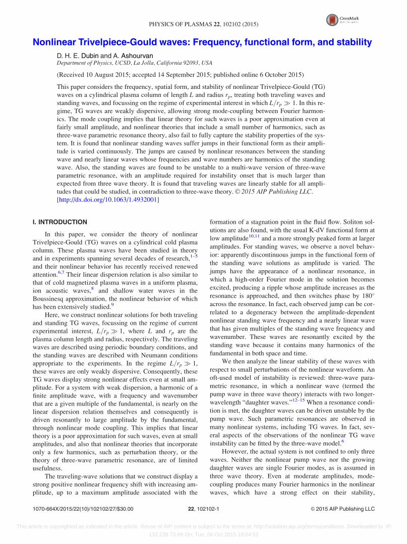
FIG. 16. Time dependence of three selected spatial Fourier harmonics, over one period of the standing wave, for k? ¼ 5 and A¼ 0.25.



132.239.73.69 On: Tue, 06 Oct 2015 18:04:52

�x2 � x0

4a21 � 6a1a2 � a2

2

16a2 2a1 � a2ð Þ þ v1;1;2 ¼ 0; (92)

�3x0N1;1;0 �x0

16þ v1;3;0 ¼ 0; (93)

x0v1;1;2 þ x0x2 � a1

a1 þ a2

16 2a1 � a2ð Þ ¼ 0; (94)

3x0v1;3;0 þa1 a1 þ a2ð Þ

16 2a1 � a2ð Þ ¼ a1N1;3;0: (95)

The solution of these equations yields the Fourier coefficients

v1;1;2 ¼ x0

a1

32a2

4a1 � 5a2

2a1 � a2

; (96)

N1;3;0 ¼2a2 � 7a1

128 2a1 � a2ð Þ ; (97)

v1;3;0 ¼ �x0

5a1 þ 2a2

128 2a1 � a2ð Þ ; (98)

as well as the lowest-order nonlinear correction to the stand-

ing wave frequency

x2 ¼ x0

2a22 þ 7a1a2 � 4a2

1

32a2 2a1 � a2ð Þ : (99)

Working to higher order, the next order correction to the fre-

quency is found to be

x4 ¼ x0½960a71 � 180a5

2a23 þ 12a1a

42a3ð�30a2 þ 47a3Þ � 64a6

1ð3a2 þ 158a3Þþ a21a

32ð396a2

2 � 4952a2a3 � 2037a23Þ

� 3a41a2ð1591a2

2 þ 7684a2a3 þ 3136a23Þþ a5

1ð�1350a22 þ 28288a2a3 þ 3264a2

3Þþ 2a3

1a22ð1434a2

2 þ 5291a2a3 þ 5517a23Þ�=½4096a2

2ð2a1 � a2Þ3ða1 � 3a3Þð3a1 � a3Þ�: (100)

Using Eqs. (82), (99), (100), and (49), the frequency of the

nonlinear standing wave can be expressed as

x=x0 ¼ 1þ 3A2

64k2?

3þ k2?

1þ k2?þ 3A4

16384k2?

135þ 69k2? þ 74k4

? þ 21k6? þ k8

?

1þ k2?

� �2þ 0 A6ð Þ:

(101)

Note that all nonlinear corrections vanish as k? ! 0. The

frequency of a nonlinear cold plasma standing wave with

k? ¼ 0 is independent of amplitude (in perturbation theory),

as discussed in Appendix A and at the end of Sec. II.

Also note that the nonlinear frequency corrections for a

standing wave are not the same as for a traveling wave, as

given by Eq. (68). In linear theory, standing waves are

merely a superposition of two counter-propagating traveling

waves and have the same dispersion as traveling waves. But

nonlinear standing waves obviously cannot be obtained as

the sum of two nonlinear traveling waves, and consequently

their dispersion differs.

In Fig. 9, we compare Eq. (101) to the frequencies found

from numerical solution of Eqs. (77) and (78). We find good

agreement provided that A and k? are sufficiently small. Just

as for the case of traveling waves, as k? increases the waves

have less dispersion to balance nonlinearity, waves of a

given amplitude A are therefore more nonlinear, and pertur-

bation expansions are less useful. Ultimately, for very large

k?, the TG waves are nearly dispersionless, and even small

amplitude waves display large deviations from linear theory.

V. LINEAR STABILITY

In this section, we examine the linear stability properties

of the nonlinear traveling and standing waves constructed in

Secs. III–IV. We first present a simple and well-known 3-

wave parametric resonance model of instability.12–15 In this

model, the nonlinear standing or traveling wave is described

as a single Fourier mode with frequency xp and wavenumber

p. (Such a model is correct only for nearly linear waves.)

This “pump” wave interacts nonlinearly with two “daughter”

waves, with frequencies xl and xm and wave numbers l and

m, respectively. These waves are assumed to initially be of

much smaller amplitude than the pump. The wave numbers

must satisfy a momentum conservation relation p ¼ lþ m.

Then when a resonance condition, xp ¼ xl þ xm, is satis-

fied, one finds that the daughter waves grow exponentially in

amplitude at the expense of the pump wave amplitude, since

a beat mode between the pump wave and one of the daughter

waves phase locks to the other daughter wave, allowing reso-

nant energy exchange.

Furthermore, for finite pump amplitude, the resonance

condition need not be perfectly satisfied, and yet this 3-wave

system is still unstable. That is, define the linear detuning of

the resonance as

Dx ¼ xl þ xm � xp; (102)

where the frequencies appearing in this expression are the

small amplitude (linear) frequencies. Recall that there is a non-

linear shift of the pump wave frequency xp due to its finite am-

plitude, see Fig. 7 or 9. There are also nonlinear shifts of

the daughter wave frequencies due to the pump. Consequently,

the detuning is changed and can in fact be reduced to zero if

the amplitude of the pump is sufficiently large, again allowing

phase locking between the waves and resonant growth of the

daughter waves at the expense of the pump wave.

However, the three-wave theory is at best a poor approx-

imation when considering nonlinear TG waves. These

waves, with k? > 1, have fairly linear dispersion and are

therefore strongly coupled to one-another by nonlinearity, as



132.239.73.69 On: Tue, 06 Oct 2015 18:04:52

we have seen in Secs. III–IV; hence, a three-wave model of

the nonlinear system is inadequate. In order to test the valid-

ity of the three-wave model and to understand the actual lin-

ear stability properties of the TG waves, we use a Fourier

representation of the perturbations on the nonlinear standing

and traveling waves.

For traveling waves, in the wave frame, there is a time-

independent equilibrium from which the system can be

perturbed to obtain linear equations of motion for the per-

turbations. The eigenmodes of these equations are found,

and growing modes are identified. However, for a given

nonlinear wave amplitude A, we find that if the Fourier rep-

resentation of the wave is sufficiently accurate, i.e., if the

number of modes M kept in the representation is sufficiently

large, none of the perturbing eigenmodes to the wave are

unstable. We find this to be true for the full range of ampli-

tudes we could study using the Fourier methods discussed

in Sec. III B. This result is in strong contradiction to the

three-wave model of parametric resonance. Furthermore,

for smaller M values where instability is observed, the most

unstable linear eigenmode bears little resemblance to either

simple single mode daughter waves, or any nonlinear trav-

eling wave or waves.

For nonlinear standing waves, the results of a linear

stability analysis are rather different. Here, there is no time-

independent equilibrium about which one can perturb.

However, since the underlying wave is periodic in time a

variant of Floquet analysis can be applied to determine the

linear eigenmodes of the perturbations. We find that if the

number of modes in the wave representation is sufficiently

large, instability is suppressed but not eliminated. Over a

range of amplitudes that depends on k?, these eigenmodes

are unstable. This range of amplitudes is in all cases far

beyond that which is predicted by the three-wave model,

and the growth rates are smaller than the three-wave

prediction.

We have tested these results using fully nonlinear nu-

merical solutions of the TG fluid equations (6)–(8) and have

found good agreement with the eigenmode stability analysis.

For the standing wave case, we find that a small seed added

to a nonlinear standing wave can grow at the expected

growth rate provided that the pump wave amplitude falls in

the range predicted by the eigenmode analysis. For traveling

waves, no growth is observed if the simulation keeps a suffi-

ciently large number of modes.

A. Traveling waves

We now consider small perturbations to nonlinear trav-

eling waves, writing

Nðs; tÞ ¼ NðsÞ þ dNðs; tÞ;Vðs; tÞ ¼ VðsÞ þ dVðs; tÞ;Uðs; tÞ ¼ UðsÞ þ dUðs; tÞ;

(103)

where s ¼ z� ut, and where NðsÞ;VðsÞ and UðsÞ satisfy the

nonlinear traveling-wave equations (13)–(15), and dN; dVand dU are perturbations to the wave. Substituting Eqs. (103)

into Eqs. (6)–(8) and linearizing yields

@

@tdN � u

@

@sdN þ @

@sNdV þ VdNð Þ ¼ 0;

@

@tdV � u

@

@sdV þ @

@sVdVð Þ ¼ � @

@sdU;

@2

@s2dU� k2

?dU ¼ �dN: (104)

We look for eigenmodes of these equations, with solutions

behaving in time as e�ixt, where x is a (possibly complex)

eigenfrequency associated with a given linear eigenmode.

Also, we expand the eigenmodes in space in a Fourier

decomposition of the same form as used in Eqs. (42)–(44)

dNðs; tÞ ¼ <e�ixtX1

m¼�1dNmeims;

dVðs; tÞ ¼ <e�ixtX1

m¼�1dVmeims: (105)

Since the coefficients in Equations (104) are real, the opera-

tion of taking the real part in Eqs. (105) can be stripped out

of the equations. Then taking a Fourier component of the

resulting equations yields

�ðxþ umÞdNm þ mX1

l¼�1ðNm�ldVl þ Vm�ldNlÞ ¼ 0;

�ðxþ umÞdVm þ mX1

l¼�1Vm�ldVl ¼ �amdNm; (106)

where Nm and Vm are Fourier coefficients of the nonlinear

traveling wave, and dNm and dVm are Fourier coefficients of

perturbations to the wave.

1. Three-wave theory

For nonlinear waves of small amplitude A, it is sufficient

to consider only three waves in the stability analysis. If the

nonlinear (pump) wave has wavenumber p, we consider its

interaction with two other linear (daughter) waves of wave-

number l and m, respectively, that satisfy p ¼ lþ m. The

pump wave is a single mode with nonzero Fourier ampli-

tudes fNp;Vpg ¼ fN�p;V�pg ¼ fA; uAg, where A is the am-

plitude (using the same notation as Sec. III B), and

u ¼ffiffiffiffiffiffiffiffiffiffiap=p

pis the phase velocity of mode p (assuming small

amplitude). Then, Eqs. (106) are reduced to four coupled

equations for the daughter wave Fourier amplitudes

�ðxþ umÞdNm þ mðNpdV�l þ VpdN�l þ dVmÞ ¼ 0;

�ðxþ umÞdVm þ mVpdV�l ¼ �amdNm;

�ðx� ulÞdN�l � lðN�pdVm þ V�pdNm þ dV�lÞ ¼ 0;

�ðx� ulÞdV�l � lV�pdVm ¼ �a�ldN�l: (107)

There is a second set of four equivalent equations involving

fdN�m; dV�mg and fdNl; dVlg, which can be obtained by

interchanging the indices m and l in Eqs. (107). Equations

(107) from a closed homogeneous set of linear equations

which have a trivial solution dNm ¼ dVm ¼ dN�l ¼ dV�l ¼ 0,



132.239.73.69 On: Tue, 06 Oct 2015 18:04:52

but for special values of x there is a nontrivial solution. It may

be found by writing Eqs. (107) as the eigenvalue problem

A Z ¼ xZ, where Z ¼ ðdNm; dVm; dN�l; dV�lÞ, and the ma-

trix A is

A ¼

�mu m muA mAam �mu 0 muA�luA �lA lu �l

0 �luA �al lu

0BB@

1CCA: (108)

The eigenvalues x of the matrix satisfy following poly-

nomial equation:

ððx� luÞ2 � x2l Þððxþ muÞ2 � x2

mÞ�A2½2lmu2ðlu� xÞðmuþ xÞ þ uðmx2

l ð3muþ 2xÞþ lx2

mð3lu� 2xÞÞ þ x2l x

2m� þA4l2m2u4 ¼ 0; (109)

where xl and xm are the frequencies of the daughter waves

in linear theory (as seen in the lab frame): xl ¼ffiffiffiffiffilal

pand

similarly for xm. The second set of four equivalent equations

mentioned in relation to Eq. (107) leads to the same result as

Eq. (109), but with l and m interchanged.

When there is no pump wave (A¼ 0), Eq. (109) has four

“unperturbed” solutions: x ¼ �mu 6 xm and x ¼ lu 6 xl,

which are frequencies of linear modes with wave numbers mand � l, respectively, traveling both to the left and to the

right (when viewed in the lab frame), and Doppler-shifted by

the pump wave phase velocity u since we are working in the

pump wave frame of reference. To each eigenfrequency is

associated an eigenvector Z ¼ ðdNm; dVm; dN�l; dV�lÞ,which is the vector of density and velocity perturbations for

that mode. For x ¼ �mu 6 xm; Z ¼ ð1;6xm=m; 0; 0Þ while

for x ¼ lu 6 xl; Z ¼ ð0; 0; 1;7xl=lÞ.The addition of a nonzero pump wave amplitude A shifts

the frequencies and mixes these unperturbed eigenvectors.

The frequency shift of the daughter waves is similar to the

nonlinear shift of the pump wave considered in Sec. III B,

except that here the shift is of the daughter waves due to the

pump, not a shift of the pump itself (which is neglected in

this analysis).

When the pump wave amplitude A is small, Eq. (109)

implies that the frequency shift of each eigenmode from its

unperturbed value is also small (of order A2), provided that

none of the four daughter wave eigenfrequencies are degen-

erate. This scaling with amplitude agrees with the scaling

found for nonlinear frequency shifts in Sec. III B. Also, the

mixing of the eigenvectors is small; i.e., each eigenmode

remains close to a daughter wave with a given wavenumber,

with only a small admixture of the other daughter wave

wavenumber. However, this changes if there is a near-

degeneracy in the eigenfrequencies, and this degeneracy can

produce strong mixing of the eigenvectors and an unstable

eigenmode.

Degeneracies occur where �mu 6 xm ¼ lu 6 xl.

Recalling that u ¼ xp=p where xp is the frequency of the

pump wave, and that p ¼ lþ m, one finds degeneracy occurs

when any of the following resonance conditions are met:

xp ¼ xl þ xm;xp ¼ xl � xm; or xp ¼ xm � xl (assuming

that xp;xl and xm are all positive). For our purposes, con-

sidering that the waves have nearly linear dispersion

(k? > 1), only the first resonance condition can be satisfied.

Then of the four eigenfrequencies, it is the two smaller fre-

quency eigenmodes that are nearly degenerate: x ��muþ xm and x � lu� xl. As seen in the lab frame, these

two eigenmodes have nearly the same phase velocity as the

pump wave if the dispersion is nearly linear. (The other two

eigenmodes have phase velocities in the opposite direction

as the pump when seen in the lab frame.) When the pump

wave amplitude is zero, the unperturbed eigenvectors for

these two near-degenerate eigenmodes are, respectively,

Z ¼ ð1;xm=m; 0; 0Þ � Z1 and Z ¼ ð0; 0; 1;xl=lÞ � Z2.

Near degeneracy, we can use degenerate perturbation

theory to describe the eigenmodes. The eigenmodes are a lin-

ear combination of Z1 and Z2

Z ¼ aZ1 þ bZ2: (110)

Thus, the perturbed density in an eigenmode has the form

dNðs; tÞ ¼ <e�ixtðaeims þ be�ilsÞ: (111)

We then project the eigenvalue equation A Z ¼ xZ,

with Z given by Eq. (110) and A by Eq. (108), onto Z1 and

Z2, obtaining a reduced eigenvalue problem for a and b

Z†1 A Z ¼ xZ

†1 Z;

Z†2 A Z ¼ xZ†

2 Z; (112)

where the dagger denotes a left eigenvector: Z†1

¼ ðxm=m; 1; 0; 0Þ and Z†2 ¼ ð0; 0;xl=l; 1Þ. Defining the

detuning from resonance as

Dx ¼ xl þ xm � xp; (113)

defining the shift of the eigenfrequency from its value on res-

onance as

dx ¼ xþ mu� xm; (114)

and assuming both Dx and dx are of order the pump ampli-

tude A (assumed small), the eigenvalue equation for a and bgiven by Eq. (112) is

0 Amx2

l þ 2pxlxm þ lx2m

2pxl

�Amx2

l þ 2pxlxm þ lx2m

2pxm�Dx

0BBB@

1CCCA

a

b

!¼ dx

a

b

!: (115)

The two solutions for the eigenfrequency shift dx are

obtained from the quadratic equation

dx2 þ Dxdxþ A2 mx2l þ 2pxlxm þ lx2

m

� �2

4p2xlxm¼ 0; (116)

which yields



132.239.73.69 On: Tue, 06 Oct 2015 18:04:52

dx ¼ 1

2�Dx6

ffiffiffiffiffiffiffiffiffiffiffiffiffiffiffiffiffiffiffiffiffiffiffiffiffiffiffiffiffiffiffiffiffiffiffiffiffiffiffiffiffiffiffiffiffiffiffiffiffiffiffiffiffiffiffiffiffiffiffiffiffiffiffiffiffiffiffiffiffiffiDx2 � A2

mx2l þ 2pxlxm þ lx2

m

� �2

p2xlxm

s0@

1A:

(117)

Equation (116) can also be obtained directly from Eq.

(109) by assuming a degeneracy for which A, Dx, and dxare all small and of the same order of magnitude.

For each solution, the coefficients a and b are related by

dxa ¼ Alx2

m þ 2pxlxm þ mx2l

2pxlb; (118)

implying that a near-degenerate eigenmode, with a and b of

roughly the same size, is a strong admixture of daughter

waves containing both wavenumbers l and m. From Eqs.

(110), (114), and (113), the density perturbation for each

eigenmode can be written as

dNðz; tÞ ¼ <ðae�iðxmþdxÞtþimz þ beiðxl�dx�DxÞt�ilzÞ; (119)

where we used s ¼ z� ut; u ¼ xp=p, and p ¼ lþ m. Note

that xl � dx� Dx can also be written as xp � xm � dx.

Thus, the sum of the two frequency components in the eigen-

mode equals xp. Physically, one frequency component in the

density beats with the pump wave to produce the other fre-

quency component, and vice versa; and therefore the fre-

quency components add to the pump wave frequency xp.

When A¼ 0, from Eqs. (117) and (118), one eigenmode

has dx ¼ 0 and b¼ 0, while the other eigenmode has dx ¼�Dx and a¼ 0, i.e., each eigenmode is a single-wavenumber

daughter wave, with frequency xm and xl, respectively, as

seen in the lab frame (see Eq. (119)). As A increases from

zero, the eigenmodes become a mixture of these daughter

waves, each with a shifted frequency �xl and �xm given by

�xl ¼ xl � Dx� dx�;

�xm ¼ xm þ dxþ;

where dx6 are the two solutions given by Eq. (116) with

corresponding 6 signs in the equation. (Here, and in what

follows, we assume Dx is a positive quantity, as is the case

for linear dispersion relation given by Eq. (12).) These can

be regarded as “natural” frequencies of the daughter waves

in the presence of the pump wave. In other words, if one

drives the three-wave system with an external potential pro-

portional to eimz�i�xmt, one will obtain a large resonant

response, and similarly for an external potential behaving as

eilz�i�x lt. However, a given eigenmode consists of one of

these two daughter waves together with the other wave

driven off of its natural frequency by an amount dxþ � dx�

(since a given eigenmode involves either dx� or dxþ, but

not both; see Eq. (119)). The natural frequency of one daugh-

ter wave interacts with the pump to produce the other daugh-

ter wave at an off-resonant frequency.

The shifted natural frequencies are plotted schematically

in Fig. 17 versus pump wave amplitude A. Each frequency is

shifted downwards as the pump wave amplitude increases. If

the amplitude becomes sufficiently large and if Dx is

sufficiently small, the sum of the two frequencies come into

resonance with the pump wave frequency, and the three-

wave system then becomes unstable.

From Eq. (117), one can see immediately that exponen-

tial growth (or decay) of the daughter waves occurs when Asatisfies

A >pjDxj ffiffiffiffiffiffiffiffiffiffiffixlxm

p


m

; (120)

with a growth (or decay) rate C given by

C ¼ 1

2

ffiffiffiffiffiffiffiffiffiffiffiffiffiffiffiffiffiffiffiffiffiffiffiffiffiffiffiffiffiffiffiffiffiffiffiffiffiffiffiffiffiffiffiffiffiffiffiffiffiffiffiffiffiffiffiffiffiffiffiffiffiffiffiffiffiffiffiffiffiffiA2


m

� �2

p2xlxm� Dx2

s: (121)

If one invokes nearly linear dispersion with xl � lu and

xm � mu, Eq. (121) simplifies further to

C ¼ 1

2

ffiffiffiffiffiffiffiffiffiffiffiffiffiffiffiffiffiffiffiffiffiffiffiffiffiffiffiffiffiffiffi9lmu2A2 � Dx2p

: (122)

Physically, instability occurs because one daughter

wave beats with the pump to produce a perturbation that res-

onantly drives the other daughter wave, and vice-versa. Even

when the linear waves are not in perfect resonance (i.e.,

Dx > 0), the nonlinear frequency shift of the daughter

waves pulls the waves into resonance with the pump wave;

see Fig. 17 (an example of the well-known phenomenon of

nonlinear frequency pulling and phase locking).

In the regime of small detuning, the growth rate is linear

in the pump amplitude. According to Eq. (122)

C ¼ 3ffiffiffiffiffilmp

uA=2; (123)

when Dx� C. This result is similar to the expression for

the growth rate for the well-known modulational instability23

for which the pump wavenumber p is assumed to be big

compared to l. Then, daughter wave l can be thought of as a

long wavelength modulation of the pump wave train, and the

FIG. 17. Schematic of the real parts of the natural frequencies �x l and �xm

for daughter waves l and m, respectively, versus pump wave amplitude A.

Also shown is the pump wave frequency xp, which is independent of A in

the three-wave model, as well as the sum of the daughter wave frequencies

(dashed curve). When the pump amplitude is sufficiently large, this sum is

shifted into resonance with the pump wave and instability results. The

growth rate C is shown schematically as the dotted-dashed curve.



132.239.73.69 On: Tue, 06 Oct 2015 18:04:52

growth rate of the modulation is, according to Ref. 23,

Cmod ¼ffiffiffiffiffiffiffiffiffiffiffiffiffiffiffiffiffiffiffiffiffiffiffi�l2x00px2A2

q, where x00p ¼ d2xp=dp2 and x2A2 ¼

3ðk?=pÞ2A2xp=4 is the lowest order nonlinear frequency

shift to the pump wave (see Eq. (68), and recall that this

expression is for p¼ 1, i.e., k? is normalized to p). Using Eq.

(12) for xp, the expression for Cmod can be written as

Cmod ¼ ð3luA=2Þk2?=

ffiffiffiffiffiffiffiffiffiffiffiffiffiffiffiffik2? þ p2

p, which has the same scaling

with A as Eq. (123). In the modulational instability, the

daughter waves (i.e., modulations) are destabilized by the

nonlinear frequency shift of the pump, whereas in the three-

wave model used here the nonlinear frequency shifts are to

the daughter waves and the shift to the pump is neglected.

Equation (123) shows that, for a given value of the

pump wavenumber p, the daughter wave l with the maxi-

mum growth rate is the one with wavenumber l ¼ p=2 (for

even p values), since m ¼ p� l. In what follows, we will

therefore focus our attention on possible instabilities driven

by a pump with p¼ 2 and with daughter wavenumbers

l ¼ m ¼ 1.

2. M wave theory

The previous three-wave analysis has the advantage of

being both analytically tractable and intuitive. However, it

leaves out several important effects. For instance, the nonlin-

ear frequency shift of the pump wave is not included in the

theory. Since this is an upward shift as amplitude Aincreases, one might then expect that nonlinear resonance

between the pump and daughter waves would occur at

smaller pump amplitude A than predicted by the three wave

theory (see Fig. 17). However, another problem is that at fi-

nite amplitude A the pump wave is not a single mode; the

nonlinear traveling wave has many Fourier components, all

of which the three-wave theory neglects. Furthermore, these

higher Fourier components become more intense as the

detuning decreases. It is therefore unclear whether a three-

wave analysis of nonlinear traveling waves that are of suffi-

ciently large amplitude to be unstable has any validity.

In fact, we will see in the following analysis that three

wave theory works to predict nonlinear frequency shifts of

the daughter waves at very small amplitude, showing the

expected downward shift in frequency, but does not work at

larger amplitudes necessary for instability according to the

three-wave theory. We find that if a sufficiently large number

of modes are kept in the following analysis, no instability

involving parametric decay to longer wavelength daughter

waves can be identified, for any pump amplitude A.

We solve the eigenvalue problem given by Eqs. (106)

numerically. We assume that only Fourier modes with

wavenumbers of magnitude less than M for some (suffi-

ciently large) value of M are required. As in the three-wave

analysis, the set of Fourier coefficients of the density and

velocity perturbations form a vector with 4M components,

Z ¼ ðdN�M; dV�M; :::; dNM; dVMÞ, (neglecting {dV0; dN0g¼ f0; 0g) such that Eq. (106) can be considered a linear

eigenvalue problem of the form A Z ¼ xZ. We therefore

require the eigenvalues and eigenvectors of the matrix A.

This numerical solution depends on an equilibrium solu-

tion for the Fourier coefficients Nm and Vm and the phase

speed u of the nonlinear traveling wave for a given value of

the transverse wavenumber k? and a given amplitude A. We

calculate the equilibrium solution for a wave with fundamen-

tal wavenumber p¼ 1 using the Fourier method described in

Sec. III B, keeping Mþ 1 Fourier mode pairs fNm;Vmg in

the wave, with �M=2 m M=2, for amplitude A and

transverse wavenumber k?=2. We then transform this solu-

tion to one with fundamental wavenumber p¼ 2 and with

2M þ 1 Fourier mode pairs, via the scale transformation

m! 2m. The transformed wave has the same amplitude Aand density components (i.e., Nm ! N2m), but half the veloc-

ity (i.e., u! u=2 and Vm ! V2m=2) and twice the transverse

wavenumber (i.e., k?=2! k?); and only the even Fourier

components are nonzero. We make this transformation with

the knowledge that a parametric resonance can now occur

between the p¼ 2 pump wave and longer wavelength l ¼m ¼ 1 daughter waves.

For example, if we take M¼ 2, we first set up a pump

wave taking transverse wavenumber k?=2 and keeping M þ1 ¼ 3 Fourier pairs, ffN�1;V�1g; fN0;V0g; fN1;V1gg, with

N0 ¼ 1;V0 ¼ 0;N1 ¼ N�1 ¼ A. This wave obeys the linear

dispersion relation u ¼ ffiffiffiffiffia1p ¼ 1=

ffiffiffiffiffiffiffiffiffiffiffiffiffiffiffiffiffiffiffiffiffiffiffiffi1þ ðk?=2Þ2

q, and

V1 ¼ V�1 ¼ uA. We then transform this to a wave with 2M þ1 ¼ 5 Fourier pairs, with half the period and twice the trans-

verse wavenumber, so that now N1 ¼ N�1 ¼ 0;V1 ¼ V�1 ¼0;N2 ¼ N�2 ¼ A;V2 ¼ V�2 ¼ uA with u ¼ 1=

ffiffiffiffiffiffiffiffiffiffiffiffiffiffiffiffi22 þ k2

?

q,

which is half the speed of the untransformed wave. A solution

of eigenvalue problem (106) then yields the same results as the

three-wave analysis presented in Sec. V A 1. The pump wave

with p¼ 2 is unstable to parametric resonance with daughter

waves l ¼ m ¼ 1 if the amplitude A exceeds the instability cri-

terion given by Eq. (120). The frequency x of the daughter

waves as seen in the moving frame displays a downward fre-

quency shift as in Fig. 17, and the frequency vanishes at insta-

bility (see Fig. 18), as expected from Eqs. (114) and (117) for

FIG. 18. The real part of the frequency x (as seen in the frame of the pump

wave) displays a downward frequency shift versus amplitude A for the low-

est frequency eigenmode on a traveling pump wave with fundamental wave-

number p¼ 2, transverse wavenumber k? ¼ 10, keeping M modes in the

stability analysis, for M ¼ 2; 20; 40; and 80. For M¼ 2, the frequency

matches the prediction of three wave theory, Eqs. (117) and (114) (dashed

line), for l ¼ m ¼ 1; p ¼ 2. For larger M, the threshold amplitude beyond

which the real frequency vanishes increases.



132.239.73.69 On: Tue, 06 Oct 2015 18:04:52

the case l ¼ m ¼ p=2. That is, in resonance, the daughter

wave eigenmodes are stationary in the frame of the pump

wave, but their amplitude grows or decays depending on the

phase relation of the eigenmode to the pump. Just below

threshold, the unstable eigenmode is a standing wave, oscillat-

ing slowly but not traveling (when viewed in the pump wave

frame), with a frequency that approaches zero as the threshold

is approached. This can be seen from Eqs. (118) and (117),

which imply that at threshold a ¼ �b.

If one increases the value of M, for given amplitude A,

one obtains a more accurate description of the nonlinear trav-

eling wave, and the number of eigenmodes described by the

system of equations also increases. We concentrate here on

the low order eigenmodes with the slowest spatial variation.

For sufficiently large values of M, these eigenmodes have

converged spatial form and converged frequency x that are

independent of further increases in M. Among these slowly

varying well-converged eigenmodes, for given values of Aand M there is never more than one unstable mode. For

M¼ 2, the instability is the three-wave resonance described

previously. For larger M, the instability appears to be a

multi-wave version of the three-wave resonance. As for the

three-wave case, as the amplitude A increases beyond a

threshold value, two eigenmode frequencies approach zero

(in the pump wave frame) and then become imaginary, one

with positive imaginary frequency (a growing mode) and the

other with negative imaginary frequency (a decaying mode).

The real part of the frequency of these modes is shown in

Fig. 18, and the imaginary part (the growth rate) is shown in

Fig. 19. The spatial form of the unstable eigenmode is shown

in Fig. 20 for three values of M, and for k? ¼ 10, at the value

of A close to the instability threshold for that M value; in

Fig. 21 the pump wave at these values of A is shown for ref-

erence. Just below the threshold value of A, these eigenmo-

des oscillate in place at a low frequency; they are standing

waves when viewed in the pump wave frame, just as in the

three wave case. The spatial form of the eigenmode is a de-

rivative of the pump wave, along with a small distortion of

the wave shape. In other words, this eigenmode is an oscilla-

tion of the two peaks of the nonlinear traveling wave toward

and away from one-other, with a small distortion of the

shape of the peaks. This is similar to a compressional wave

on a chain of particles. For amplitudes just beyond instabil-

ity, the shift in position of the two peaks grows exponentially

as the peaks distort in shape.

It is not surprising that the frequency of such an eigen-

mode approaches zero at large amplitude. At large ampli-

tudes, we have seen that the traveling wave becomes a series

of sharp peaks similar to a train of solitons; see Fig. 21.

These near-solitons are rather far apart with respect to their

width, and thus interact only weakly with one another.

Hence, their locations can be changed slightly with respect

to one another without inducing much restoring force.

Note however, that the threshold value of the amplitude

A necessary for instability increases as M increases; see Figs.

18 and 19. In fact, for sufficiently large M, all amplitudes A

FIG. 20. The unstable density eigenmode near the lowest value of A for which instability occurs, for three values of M and for k? ¼ 10. (a) M ¼ 20;A ¼ 0:05,

(b) M ¼ 40;A ¼ 0:065, and (c) M ¼ 80;A ¼ 0:085.

FIG. 21. Density versus position in a traveling wave with fundamental

wavenumber p¼ 2 and k? ¼ 10, for three amplitudes corresponding to the

eigenmodes shown in Fig. 20: A¼ 0.05 (dotted-dashed), A¼ 0.065 (solid),

and A ¼ 0:085 (dashed).

FIG. 19. The growth rate C for the unstable eigenmode on a nonlinear trav-

eling pump wave with fundamental wavenumber p¼ 2 versus the amplitude

A of the traveling wave, keeping M modes in the stability analysis, and for

k? ¼ 10. The M¼ 2 case is compared to the prediction of three wave theory

(the solid line), Eq. (122), with l ¼ m ¼ 1 and p¼ 2.



132.239.73.69 On: Tue, 06 Oct 2015 18:04:52

of physical relevance are stable. For M¼ 640, the maximum

value employed in our calculations, and for k? ¼ 10, the

growth rate vanishes for A values up to A¼ 0.12. This value

of A corresponds to a maximum density in the wave of

roughly 4.8, which is far beyond any experimentally relevant

density for a nonlinear traveling TG wave.

While the results presented here are for k? ¼ 10, we

find no qualitative difference with results for any other value

of k? we have tested. For sufficiently large M, none of the

well-converged eigenmodes are unstable; and the least stable

(lowest frequency) eigenmodes have forms similar to those

shown in Fig. 20.

Thus, we find that if the numerical resolution of a non-

linear traveling TG wave is sufficiently fine, the waves are

linearly stable. The three-wave theory is not relevant to

these waves because when k? > 1 they contain many

Fourier modes, obviating an analysis based on a small num-

ber of modes.

B. Standing waves

We now turn our attention to the linear stability of non-

linear standing waves. We consider linear perturbations to a

nonlinear periodic standing wave that satisfies Eqs.

(73)–(76). The perturbations satisfy linearized versions of

Eqs. (73) and (74)

d _Nm tð Þ þ m

2

X1m0¼1

dVm0 Nm�m0 þ Nm0�m � Nmþm0½ �

þVm0 dNm�m0 þ dNm0�m � dNmþm0½ �g ¼ 0; (124)

d _Vm tð Þ þ 1

2

X1m0¼1

m0 dVm0 Vm�m0 � Vm0�m þ Vmþm0½ �

þVm0 dVm�m0 � dVm0�m þ dVmþm0½ �g ¼ amdNm; (125)

where NmðtÞ and VmðtÞ are the Fourier coefficients of the

nonlinear standing wave, and dNmðtÞ and dVmðtÞ are the per-

turbed Fourier coefficients of the wave.

While these coupled ordinary differential equations are

linear in the unknown functions dNm and dVm, the coeffi-

cients in the equations have periodic time dependence, which

complicates their solution compared to the traveling-wave

case. We first consider an analytic approach to the solution

via two-timescale analysis applied to three waves, and then

consider a numerical approach based on Floquet analysis for

the general M waves case.

1. Three wave theory

For nonlinear standing waves of small amplitude A, it is

sufficient to consider only three waves in the stability analy-

sis. As in the traveling-wave case, let the nonlinear pump

wave have wavenumber p and the two linear daughter waves

have wave numbers l and m, where p ¼ lþ m. The pump

wave again is described as a single Fourier mode with the

following Fourier coefficients of a linear standing wave:

fNpðtÞ;VpðtÞg ¼ AfcosðxptÞ; ðxp=pÞ sinðxptÞg; (126)

where xp ¼ffiffiffiffiffiffiffipapp

is the frequency of the pump wave. Then

Eqs. (124) and (125) reduce to

d _Nm tð Þ þ m

2�Np tð ÞdVl þ Vp tð ÞdNl þ 2dVm

� �¼ 0; (127)

d _Vm tð Þ � m

2Vp tð ÞdVl

� �¼ amdNm; (128)

together with equations for dNl and dVl that can be obtained

from Eqs. (127) and (128) by interchanging l and m.

We will solve these equations approximately, assuming

that the detuning Dx given by Eq. (113) is small, of order A.

Then a consistent solution has the form

dNmðtÞ ¼ nmðsÞe�ixmt þ c:c:; (129)

dVmðtÞ ¼ vmðsÞe�ixmt þ c:c:; (130)

and similarly for dNl; dVl, where c:c: denotes complex conju-

gate, s ¼ At is a slow time variable, and nmðsÞ and vmðsÞ are

slowly varying amplitudes for the daughter waves.

Substituting these equations as well as Eq. (126) into Eqs.

(127) and (128), we consider terms which vary in time like

e�ixmt and divide through by this factor, to obtain the follow-

ing slow timescale equations:

�ixmnm þ mvm þ Ad

dsnm �

mA

4v�l �

ixp

pn�l

� �eiDxs=A ¼ 0;

(131)

�ixmvm � amnm þ Ad

dsvm �

imAxp

4pv�l eiDxs=A ¼ 0: (132)

To zeroth order in A, these equations imply that nm

¼ �imvm=xm and x2m ¼ mam, which are the relations for lin-

ear waves. Similarly, one also has n�l ¼ ilv�l =xl to lowest

order in A (which follows from Eq. (131) with m and l inter-

changed). To first order in A, we may use these relations in

the terms proportional to A in Eqs. (131) and (132). However,

in the zeroth-order parts of the equations, we must keep a

first-order correction, writing nm ¼ �imvm=xm þ ADnm.

Then, Eqs. (131) and (132) become

�ixmADnm � iAm

xm

d

dsvm �

mA

4v�l 1þ lxp

pxl

� �eiDxs=A ¼ 0;

(133)

�amADnm þ Ad

dsvm �

imAxp

4pv�l eiDxs=A ¼ 0: (134)

Then, multiplying Eq. (133) by �ixm=m and adding the

result to Eq. (134) yield

� x2m

mþ am

� �Dnm þ

im

4v�l

xm

mþ lxpxm

mpxl� xp

p

� �¼ 0:

(135)

Substituting the solution of this equation for Dnm into Eq.

(134), and using the linear dispersion relation x2m ¼ mam,

then yields the slow time equation



132.239.73.69 On: Tue, 06 Oct 2015 18:04:52

d

dsvm � iclv

�l eiDxs=A ¼ 0; (136)

where

cl ¼pxlxm þ mxlxp þ lxmxp

8pxl: (137)

Equation (136) is coupled to the slow-time equation for vl,

which is the same as Eq. (136) but with l and m interchanged

d

dsvl � icmv�meiDxs=A ¼ 0: (138)

Writing vmðsÞ ¼ ðxmðsÞ þ iymðsÞÞeiDxs=2A, where xm and ym

are real functions, and similarly for vlðsÞ, we can convert

Eqs. (136) and (138) into four coupled real ordinary differen-

tial equations for xm; ym; xl; and yl

_xm sð Þ � Dx2A

ym � clyl ¼ 0; (139)

_ym sð Þ þ Dx2A

xm � clxl ¼ 0; (140)

_xl sð Þ � Dx2A

yl � cmym ¼ 0; (141)

_yl sð Þ þ Dx2A

xl � cmxm ¼ 0: (142)

Assuming that xmðsÞ ¼ <x0meCss, and similarly for the other

three unknown functions, allows determination of the slow

timescale rate Cs from the determinant of the resulting ma-

trix equation. The result is C2s ¼ clcm � Dx2=ð4A2Þ.

Converting this variable to a fast-timescale rate C ¼ ACs

(i.e., writing xm in terms of t rather than s as xm ¼ <x0meCtÞthen yields the growth (or decay) rate in the three wave

theory

C ¼ 1

2

ffiffiffiffiffiffiffiffiffiffiffiffiffiffiffiffiffiffiffiffiffiffiffiffiffiffiffiffiffiffi4A2clcm � Dx2

p: (143)

The rate is real provided that 4A2clcm > Dx2, otherwise the

rate is imaginary and the daughter waves oscillate in ampli-

tude rather than growing or decaying. This instability onset

is similar to that found in the three wave theory for traveling

waves, Eq. (120). When the dispersion is nearly linear with

xm � um for all m, Eq. (143) simplifies to

C ¼ 1

2

ffiffiffiffiffiffiffiffiffiffiffiffiffiffiffiffiffiffiffiffiffiffiffiffiffiffiffiffiffiffiffiffiffiffiffiffiffiffi9A2lmu2=16� Dx2

p; (144)

which is identical to the traveling-wave growth (or decay)

rate in the nearly linear dispersion regime, Eq. (122), except

for a factor of 4 dividing A. This factor can be traced to the

difference in the definition of A in the traveling and standing

wave cases: for the traveling wave, the pump wave has the

form Np ¼ A exp½iðpz� xptÞ� þ c:c:, whereas in the standing

pump wave has the form Np ¼ A cosðpzÞ cosðxptÞ ¼ ðA=4Þfexp½iðpz� xptÞ� þ exp½iðpzþ xptÞ�g þ c:c:; so the standing

pump wave is two counter-propagating traveling waves,

each with amplitude A=4. Each traveling pump wave

interacts with daughter waves with nearly the same phase

velocity, and their interaction with the counter-propagating

waves can be neglected in three-wave theory.

Thus, in the three-wave theory, the standing wave and

its accompanying daughter waves can be treated as a super-

position of essentially independent counter-propagating

traveling waves, just as in linear theory. However, in the

M-wave theory presented below, we will find that this is not

true—the stability properties of a nonlinear standing wave

differ from those of traveling waves.

2. M wave theory

We now solve Eqs. (124) and (125) for an arbitrary

number of Fourier modes using a variant of Floquet theory.

For a given nonlinear standing wave with amplitude A and

frequency x, we first assume that dNm ¼ 0 and dVm ¼ 0 for

m>M, for some (sufficiently large) value of M. We then

construct a vector of unknown Fourier coefficients

Z ¼ fdN1; dV1; :::; dNM; dVMg, and note that Eqs. (124) and

(125) can be expressed in vector form as _Z ¼ AðtÞ Z,

where the matrix AðtÞ is periodic with period T ¼ 2p=x.

Now, consider a solution Zðt;Z0Þ of these differential equa-

tions for a given initial condition Z0. The homogeneous lin-

ear form of the differential equations implies that

Zðt;Z0Þ ¼ LðtÞ Z0; (145)

where the matrix LðtÞ is a linear transformation that takes

the initial condition to the solution at time t. In particular, let

us consider the solution integrated over one period T of the

standing wave and define Z1 ¼ ZðT;Z0Þ. Then

Z1 ¼ LðTÞ Z0; (146)

where the matrix LðTÞ has real coefficients. If we now inte-

grate the differential equations starting at time t¼ T with ini-

tial condition Z1 and ending one period later, at time t ¼ 2T,

at Z2, we will find that Z2 ¼ LðTÞ Z1 because the matrix

AðtÞ is periodic and therefore has the same time dependence

as in the previous integration. Proceeding to integrate ntimes, we find that

Zn ¼ LðTÞn Z0; (147)

where Zn ¼ Zðt ¼ nT;Z0Þ. Thus, stability of the system of

equations is determined by the size of the eigenvalues k of

the matrix LðTÞ. Any eigenvalue with magnitude greater

than unity causes exponential growth in the solution.

However, the product of the eigenvalues equals unity,

because the equations of motion are conservative. Thus, any

eigenvalue with magnitude greater than one must be bal-

anced by eigenvalues with magnitudes less than one.

The accompanying eigenvector Z0j to an eigenvalue kj

with magnitude greater than one provides the functional

form of the growing eigenmode at the instants of time

t ¼ nT; n ¼ 0; 1; 2; :::. In between these times, the mode may

have a quite complex time dependence, but returns to the

form predicted by the eigenvector each period. Thus, the

time dependence of the jth eigenmode ZjðtÞ corresponding to

eigenvector Z0j has the following form:



132.239.73.69 On: Tue, 06 Oct 2015 18:04:52

ZjðtÞ ¼ kt=Tj ZejðtÞ; (148)

where ZejðtÞ is a continuous (in time) periodic vector with pe-

riod T that equals Z0j at times t ¼ nT. This vector can be writ-

ten explicitly as Ze;jðtÞ ¼ kFloorðt=TÞ�t=Tj Lðmodðt; TÞÞ Z0j,

where FloorðxÞ is the integer nearest to but less than x.

In order to test the stability of a given standing wave, we

determine the matrix LðTÞ by solving Eqs. (124) and (125)

numerically over a single period T of the wave, for 2M dif-

ferent initial conditions. For the first initial condition, we

take Z0 ¼ f1; 0; 0; :::g. The vector Z1 determined by the nu-

merical integration of the equations provides us with the first

column of the matrix LðTÞ, according to Eq. (146). The next

initial condition Z0 ¼ f0; 1; 0; 0; ::g determines the next col-

umn of LðTÞ, and so on. Once we have found LðTÞ in this

way, we evaluate the eigenvalues kj; j ¼ 1; ::; 2M, to deter-

mine stability. The exponential growth rate C associated

with an eigenvalue k is then

C ¼ lnðjkjÞ=T: (149)

However, we limit ourselves to the set of eigenvalues that

are well-converged, i.e., that do not vary with increasing M,

for M sufficiently large. (Values of M up to 120 were

employed.) Also, as for the traveling waves, we consider

only standing waves with fundamental wavenumber p¼ 2,

for a range of amplitudes and for several k? values: k? ¼4; 5; 6; 10; and 20. We find that, among the converged eigen-

values, for a given amplitude A and value of k?, either zero,

one, or two eigenvalues have magnitudes larger than unity,

and hence have nonzero growth rate C. When there is one

such eigenvalue, it is real and negative, and the associated

eigenvector Z0j is also real. When there are two such eigen-

values, they are complex and are conjugate to one-another,

and so are the eigenvectors. This implies that the growth

rates for these two eigenvectors are identical.

In Fig. 22, we display numerical results for C versus the

amplitude A of a standing wave with fundamental wavenum-

ber p¼ 2, k? ¼ 10, and for several values of M. The standing

wave is also evaluated using M Fourier modes, using the

methods of Sec. IV. Since its fundamental wavenumber is

p¼ 2, the standing wave has only even Fourier components.

The unstable mode has only odd components.

For M¼ 2, the calculated growth rate agrees with the

rate given by three wave analysis, Eq. (143), taking daughter

waves with l ¼ m ¼ 1 and a pump wave with p¼ 2 (the

dashed curve in the figure). For larger M, we observe a sup-

pression of the growth rate similar to what was found for

traveling waves. However, the converged growth rate found

for sufficiently large M (the solid line) values does not van-

ish. While much reduced from the three wave theory, the

growth rate remains finite for a range of A values.

Some of the growth rate values displayed in Fig. 22 cor-

respond to a single real eigenmode with a negative eigen-

value, and others correspond to a complex-conjugate pair of

eigenmodes with equal growth rates. The case of a single

negative eigenvalue corresponds to a growing, oscillating

perturbation which changes sign each period of the standing

wave; i.e., a growing oscillation with exactly half the oscilla-

tion frequency of the standing wave, and phase-locked to the

wave, just as for the three-wave theory. However, unlike

three-wave theory, the functional form of the unstable eigen-

mode is not a single spatial Fourier mode. An example is dis-

played in Fig. 23 for A¼ 0.22. The unstable density and

velocity perturbation at the instant of maximum standing

wave amplitude is displayed in (a), along with the standing

wave at that instant, in (b). One period T later the perturba-

tion changes sign and grows by the factor jkj. An animation

of the time dependence of the perturbation over two cycles

FIG. 23. (a) The unstable density eigenmode (dashed) and velocity eigenmode (solid) for a p¼ 2 standing wave with A¼ 0.22 and k? ¼ 10, at an instant of

maximum amplitude of the wave. (b) The standing wave density at the same instant. Both evaluations were carried out for M¼ 80. An animation of the per-

turbed density and the standing wave over two periods of the wave is supplied in the online material. (Multimedia view) [URL: http://dx.doi.org/10.1063/

1.4932001.1]

FIG. 22. Instability growth rate C for a standing wave with fundamental

wavenumber p¼ 2 versus amplitude A, for k? ¼ 10, and for increasing reso-

lution of both the standing wave and the perturbations, from M¼ 2 to

M¼ 32 (dots). Also shown is the growth rate predicted by three-wave theory

taking m ¼ l ¼ 1 and p¼ 2 in Eq. (143) (dashed), and the converged growth

rate (solid) evaluated for M up to 120.



132.239.73.69 On: Tue, 06 Oct 2015 18:04:52

http://dx.doi.org/10.1063/1.4932001.1

http://dx.doi.org/10.1063/1.4932001.1

of the standing wave can be found in the online material.

These eigenfunctions are converged to within about one part

in 10�3. The spatial oscillations in the eigenmode are not

artifacts of the finite number of Fourier modes kept in the

expansion.

The functional form of the eigenmodes for a case for

which there are two complex-conjugate unstable eigenvalues,

A¼ 0.26 and k? ¼ 10, is displayed in Fig. 24. The eigenval-

ues in this case are k ¼ �1:0314860:16398i and are well-

converged to an accuracy of at least 10�5. The two unstable

complex-conjugate eigenmodes grow at the same rate. The

unstable density and velocity perturbations at an instant of

maximum standing wave amplitude are displayed in (a) and

(b), corresponding to the real and imaginary parts, respec-

tively, of the eigenvector for which =k > 0. For the other

unstable eigenvector, the real part (a) is the same and the

imaginary part (b) has opposite sign. The standing wave at

the same instant of maximum amplitude is displayed in (c).

The real part of the eigenmode is somewhat similar in form to

the case shown in Fig. 23. The imaginary part of the eigen-

mode is rather different in form (although its density perturba-

tion may not be fully converged at our maximum resolution

of M¼ 120).

In Fig. 25, we display the converged growth rate of the

unstable mode(s) versus standing wave amplitude for all val-

ues of k? studied. As k? decreases, the amplitude required for

instability increases. Evidently, the larger dispersion of waves

with smaller k? increases the amplitude required for mode

coupling and instability. This is expected even in the three

wave theory, but the required amplitude we observe is consid-

erably larger than three wave theory would predict.

For example, for k? ¼ 5 or less, no instability in con-

verged eigenmodes is observed, up to the maximum ampli-

tude tested, A ¼ 0:52, corresponding to a maximum density at

k? ¼ 5 of Nmax ¼ 3:8 (the onset of instability at k? ¼ 5 is

predicted by three-wave theory to be at A¼ 0.14; see Eq.

(144)). For k? ¼ 6, there is a single unstable eigenmode for

amplitudes in the range 0:32 < A < 0:34 (the first peak),

while for larger A values (the second peak) there are two

complex-conjugate unstable eigenmodes. For k? ¼ 10, there

is a single unstable eigenmode for amplitudes in the range

0:17 < A < 0:25 (the first peak), while for larger A values

there are two unstable complex-conjugate eigenmodes. For

k? ¼ 20, the growth rate results have a rather complicated

structure. There is a single unstable eigenmode for amplitudes

in the ranges 0:092 < A < 0:127 and 0:139 < A < 0:14, and

there are two complex-conjugate unstable modes in the ranges

0:128 < A < 0:131 and 0:141 < A < 0:145. We emphasize

that this complicated structure is not the result of numerical

noise; the growth rates are well converged for all amplitude

values shown. Some of the structure can be associated with

the previously discussed jumps in the density of the standing

wave. For instance, the first appearance of unstable modes at

A¼ 0.092 occurs at the leftmost density jump shown in Fig.

13 (recall that the p ¼ 1; k? ¼ 10 standing wave considered

in Fig. 13 can be mapped by a scale transformation to the p ¼2; k? ¼ 20 wave considered in Fig. 25).

In Fig. 26, we display the growth rates versus the scaled

amplitude 3uA=4Dx, which in three-wave theory equals unity

at the instability onset for all k? � 1 (see Eq. (144)). One can

see that as k? increases, the scaled amplitude required for

instability increases as well. This is because as k? increases,

the dispersion becomes more linear at a given amplitude so

there is more mode-coupling that increases the harmonic con-

tent of both the standing wave and the growing eigenmode,

making 3 wave theory a less-relevant approximation.

We have tested these results by simulating the full non-

linear fluid equations, Eqs. (6)–(8). Details of the simulation

method are described in Appendix B. In one set of simula-

tions, we begin the simulation with a standing wave with

fundamental wavenumber p¼ 2 at a given amplitude, to

FIG. 24. The real (a) and imaginary part (b) of the unstable density eigenmodes (dashed) and velocity eigenmodes (solid) for a p¼ 2 standing wave with

A¼ 0.26 and k? ¼ 10, at the instant of maximum amplitude of the wave. The growth rate for both eigenmodes is identical: C ¼ 1:498 10�3 (see Fig. 22). (c)

The standing wave density at the same instant. Evaluations were carried out for M¼ 120.

FIG. 25. Converged growth rate (dots connected by lines) versus amplitude

A for standing waves with fundamental wavenumber p¼ 2, and for several

values of k?. The X’s are growth rates determined through simulation of the

fluid equations, by adiabatically driving a standing wave to the given ampli-

tude and seeding it with a small m¼ 1 Fourier mode.



132.239.73.69 On: Tue, 06 Oct 2015 18:04:52

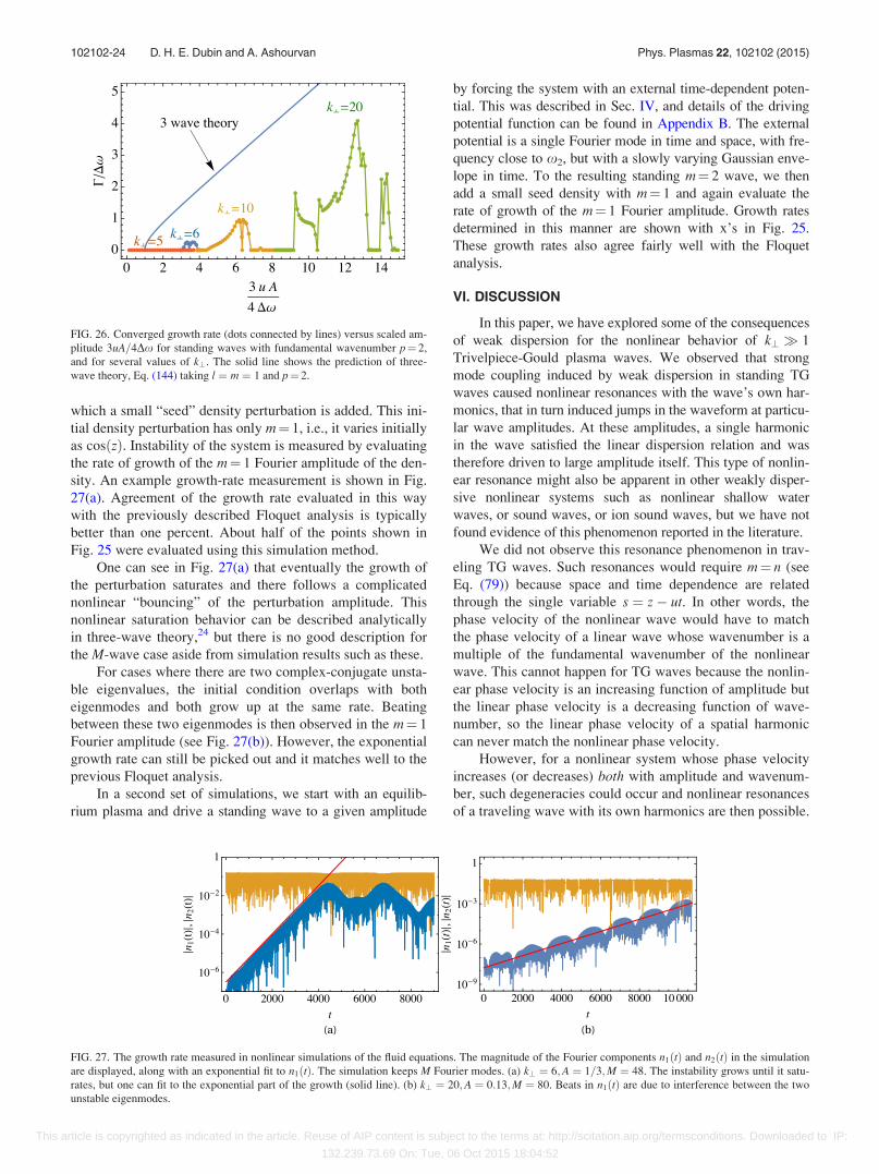
which a small “seed” density perturbation is added. This ini-

tial density perturbation has only m¼ 1, i.e., it varies initially

as cosðzÞ. Instability of the system is measured by evaluating

the rate of growth of the m¼ 1 Fourier amplitude of the den-

sity. An example growth-rate measurement is shown in Fig.

27(a). Agreement of the growth rate evaluated in this way

with the previously described Floquet analysis is typically

better than one percent. About half of the points shown in

Fig. 25 were evaluated using this simulation method.

One can see in Fig. 27(a) that eventually the growth of

the perturbation saturates and there follows a complicated

nonlinear “bouncing” of the perturbation amplitude. This

nonlinear saturation behavior can be described analytically

in three-wave theory,24 but there is no good description for

the M-wave case aside from simulation results such as these.

For cases where there are two complex-conjugate unsta-

ble eigenvalues, the initial condition overlaps with both

eigenmodes and both grow up at the same rate. Beating

between these two eigenmodes is then observed in the m¼ 1

Fourier amplitude (see Fig. 27(b)). However, the exponential

growth rate can still be picked out and it matches well to the

previous Floquet analysis.

In a second set of simulations, we start with an equilib-

rium plasma and drive a standing wave to a given amplitude

by forcing the system with an external time-dependent poten-

tial. This was described in Sec. IV, and details of the driving

potential function can be found in Appendix B. The external

potential is a single Fourier mode in time and space, with fre-

quency close to x2, but with a slowly varying Gaussian enve-

lope in time. To the resulting standing m¼ 2 wave, we then

add a small seed density with m¼ 1 and again evaluate the

rate of growth of the m¼ 1 Fourier amplitude. Growth rates

determined in this manner are shown with x’s in Fig. 25.

These growth rates also agree fairly well with the Floquet

analysis.

VI. DISCUSSION

In this paper, we have explored some of the consequences

of weak dispersion for the nonlinear behavior of k? � 1

Trivelpiece-Gould plasma waves. We observed that strong

mode coupling induced by weak dispersion in standing TG

waves caused nonlinear resonances with the wave’s own har-

monics, that in turn induced jumps in the waveform at particu-

lar wave amplitudes. At these amplitudes, a single harmonic

in the wave satisfied the linear dispersion relation and was

therefore driven to large amplitude itself. This type of nonlin-

ear resonance might also be apparent in other weakly disper-

sive nonlinear systems such as nonlinear shallow water

waves, or sound waves, or ion sound waves, but we have not

found evidence of this phenomenon reported in the literature.

We did not observe this resonance phenomenon in trav-

eling TG waves. Such resonances would require m¼ n (see

Eq. (79)) because space and time dependence are related

through the single variable s ¼ z� ut. In other words, the

phase velocity of the nonlinear wave would have to match

the phase velocity of a linear wave whose wavenumber is a

multiple of the fundamental wavenumber of the nonlinear

wave. This cannot happen for TG waves because the nonlin-

ear phase velocity is an increasing function of amplitude but

the linear phase velocity is a decreasing function of wave-

number, so the linear phase velocity of a spatial harmonic

can never match the nonlinear phase velocity.

However, for a nonlinear system whose phase velocity

increases (or decreases) both with amplitude and wavenum-

ber, such degeneracies could occur and nonlinear resonances

of a traveling wave with its own harmonics are then possible.

FIG. 27. The growth rate measured in nonlinear simulations of the fluid equations. The magnitude of the Fourier components n1ðtÞ and n2ðtÞ in the simulation

are displayed, along with an exponential fit to n1ðtÞ. The simulation keeps M Fourier modes. (a) k? ¼ 6;A ¼ 1=3;M ¼ 48. The instability grows until it satu-

rates, but one can fit to the exponential part of the growth (solid line). (b) k? ¼ 20;A ¼ 0:13;M ¼ 80. Beats in n1ðtÞ are due to interference between the two

unstable eigenmodes.

FIG. 26. Converged growth rate (dots connected by lines) versus scaled am-

plitude 3uA=4Dx for standing waves with fundamental wavenumber p¼ 2,

and for several values of k?. The solid line shows the prediction of three-

wave theory, Eq. (144) taking l ¼ m ¼ 1 and p¼ 2.



132.239.73.69 On: Tue, 06 Oct 2015 18:04:52

Certain optical systems are of this type; for example, an opti-

cal system with refractive index that increases with fre-

quency and with amplitude (through the optical Kerr effect).

Harmonic generation in these systems could make use of

such resonances. In particular, for optical frequency-

doubling, resonance occurs when the “phase-matching”

requirement

Nð2x; 0Þ ¼Nðx;AÞ;

is met, where Nðx;AÞ is the frequency-and-intensity-

dependent refractive index of a nonlinear medium through

which the light travels (and here A is the intensity of a beam

of frequency x that is to be frequency-doubled in the nonlin-

ear medium). [This phase-matching requirement is equivalent

to the condition that the phase velocity of the frequency-

doubled wave matches that of the fundamental.] Nonlinearity

of the refractive index could then be used to produce strong

harmonic generation by satisfying this resonance condition

with a high intensity pump wave.

However, the intensity dependence of the index is typi-

cally too weak to be of much importance in the resonance

condition (at the intensities of interest in most applications),

so that the linear refractive index Nðx; 0Þ is a good approxi-

mation for the right side of the equation.25 In this case, the

phase-matching requirement is satisfied using other effects,

such as birefringence, or periodic poling, in an anisotropic

medium such as a uniaxial crystal.26

We observed that mode coupling in TG waves reduced

instability of the waves due to parametric resonance. For

traveling waves, instability is completely suppressed, while

for standing waves, the amplitude threshold necessary for

instability onset is several times the prediction of three-wave

theory (depending on k?), and the growth rate is smaller.

One important aspect of the stability calculations pre-

sented here is that, in order to obtain converged growth rates,

a great many Fourier harmonics had to be included in the

calculations, especially at larger amplitudes. However, the

cold fluid theory we have used could be a poor approxima-

tion for the higher harmonics, depending on parameters not

included in the theory such as temperature or viscosity. In

experiments that observe parametric instability in TG modes,

such high harmonics could be Landau-damped, damped

through collisions, or shifted in their resonant frequency by

finite thermal pressure or finite plasma radius effects. A

more realistic theory, incorporating these effects, will prob-

ably be needed to make contact with current experiments,

since the wave dynamics is apparently quite sensitive to the

number of harmonics that actually participate.

In addition, the use of Neumann boundary conditions

for the wave potential is problematic for large amplitude

standing waves in the current experiments on finite length

plasmas, as this approximation neglects the motion of the

plasma ends, which has an important influence on the reflec-

tion of the waves.

ACKNOWLEDGMENTS

The authors benefited from useful discussions with

Professor T. O’Neil, Professor C. F. Driscoll, and Professor H.

Milchberg; Dr. F. Anderegg and Dr. John Bollinger; and Matt

Affolter. The research was supported by National Science

Foundation Grant No. PHY-1414570, and Department of

Energy Grant Nos. DE-SC0002451 and DE-SC0008693.

APPENDIX A: THE k?50 CASE: COLD LANGMUIRWAVES

The k? ¼ 0 limit of Eqs. (6)–(8) admits a general ana-

lytic solution in Lagrangian coordinates. Equations (6) and

(7) can be written as

dN

dt¼ �N

@V

@z; (A1)

dV

dt¼ � @U

@z; (A2)

where the total time derivative along a Lagrangian trajectory

is d=dt ¼ @=@tþ V@=@z. Introducing the inverse density

variable U ¼ 1=N, and taking a second total time derivative

of Eq. (A1), yields

d2U

dt2¼ U

@V

@z

� �2

þ Ud

dt

@V

@z: (A3)

However, the derivatives in the last term in Eq. (A3) can be

exchanged

d

dt

@V

@z¼ @2V

@t@zþ V

@2V

@z2

¼ @

@z

dV

dt� @V

@z

� �2

: (A4)

When Eq. (A4) is substituted in Eq. (A3), and Eq. (A2) is

employed, the result is

d2U

dt2¼ �U

@2U@z2

¼ 1� U; (A5)

where in the last step Eq. (8) was applied, taking k? ¼ 0.

Equation (A5) is a harmonic oscillator equation with solution

U ¼ 1þ C cosðtþ wÞ, where C and w are constants of inte-

gration that depend on the initial conditions (i.e., they are

functions of the initial position z0 of a fluid element).

Thus, in the Lagrangian picture, the density oscillates

with unit frequency (that is, at the plasma frequency), inde-

pendent of the spatial form or amplitude of the initial condi-

tions as given by Cðz0Þ and wðz0Þ (which determine the

initial density and velocity fields). (Note that an arbitrary

constant velocity can be added to the velocity field, which

causes a Doppler shift to the oscillation frequency that is not

apparent in Eq. (A5) because this equation is valid in the

frame of the fluid flow.) However, this solution is valid only

provided that the characteristics zðz0; tÞ do not cross, which

requires jCj < 1; otherwise the density and velocity field

become ill-defined. [The characteristics can be found by

solving dz=dt ¼ Vðz; tÞ with initial condition z¼ z0.] Thus,

provided that oscillation amplitudes are small enough so that



132.239.73.69 On: Tue, 06 Oct 2015 18:04:52

jCj < 1, all solutions of the k? ¼ 0 cold fluid equations sim-

ply oscillate at the plasma frequency, independent of their

spatial form.

APPENDIX B: SIMULATION OF THE FLUIDEQUATIONS

Numerical solutions to Eqs. (6)–(8) were evaluated

using the Galerkin method, by expanding the density, veloc-

ity, and potential in spatial Fourier modes

Nðz; tÞ ¼XM

m¼�M

nmðtÞeimz;

Vðz; tÞ ¼XM

m¼�M

vmðtÞeimz;

Uðz; tÞ ¼XM

m¼�M

/mðtÞeimz;

(B1)

dropping Fourier coefficients for jmj > M, and taking

n0ðtÞ ¼ 1;/0ðtÞ ¼ v0ðtÞ ¼ 0. Reality of the density implies

that n�mðtÞ ¼ n�mðtÞ, and similarly for the velocity and

potential. Using this Fourier expansion, Eqs. (6)–(8)

become coupled ordinary differential equations for the

Fourier coefficients

_nmðtÞ þ imXM

l¼�M

nlðtÞvm�lðtÞ ¼ 0; (B2)

_vmðtÞ þ iXM

l¼�M

lvlðtÞvm�lðtÞ ¼ �iamnmðtÞ: (B3)

Equations (B2) and (B3) can then be integrated for given ini-

tial conditions, for 1 m M. Depending on the initial con-

ditions, either traveling waves or standing waves can be

simulated using these equations. For example, for standing

waves, we choose initial conditions with nmð0Þ real and

vmð0Þ imaginary. The form of the equations then guarantees

that nmðtÞ will remain real and vmðtÞ will remain imaginary

for all t, and the reality conditions then imply that n�mðtÞ ¼nmðtÞ and v�mðtÞ ¼ �vmðtÞ so that the density has a cosine

Fourier expansion and the velocity a sine expansion, as in

Eqs. (69) and (70).

In some simulations, we drive the system with an exter-

nal potential in order to produce a nonlinear standing wave.

In this case, we modify Eq. (B3) to read

_vmðtÞ þ iXM

l¼�M

lvlðtÞvm�lðtÞ ¼ �iamnmðtÞ � im/extmðtÞ; (B4)

where /extmðtÞ is the Fourier coefficient of the external

potential. This mimics experiments that create standing

waves in the plasma column by driving a potential on exter-

nal electrodes surrounding the plasma. In order to drive a

standing wave with fundamental wavenumber p, we take the

following form for this potential:

/extmðtÞ ¼ �e�ðt�t0Þ2=Dt2 sinðXtÞdm;p: (B5)

The frequency X is chosen at, or slightly above, the linear

frequency of the fundamental mode, and the time Dt is cho-

sen so that XDt� 1, so that the wave is driven to large am-

plitude adiabatically. This allows time for all of the

harmonics in the standing wave to couple to the fundamen-

tal. The time t0 is chosen to be greater than 3Dt. The ampli-

tude parameter � along with Dt determine the ultimate size of

the resulting standing wave. There is an art to choosing these

parameters. If Dt is too large, the wave will be driven up and

then back down as nonlinearity changes the response of the

system to the forcing. If Dt is too small, the resulting wave

will not have the correct harmonic content for a standing

wave of the given amplitude. The resulting wave is also sen-

sitive to the value of X, particularly at larger amplitudes.

Table I shows the values of parameters used in some of the

simulations of p¼ 2 standing waves, as well as the amplitude

A of the resulting wave.

These standing waves can then be seeded with a small

amplitude m¼ 1 Fourier mode in order to test stability. The

growth rates resulting from such tests are displayed as the

X’s in Fig. 25.

1A. W. Trivelpiece and R. W. Gould, J. Appl. Phys. 30, 1784 (1959).2J. H. Malmberg and C. B. Wharton, Phys. Rev. Lett. 17, 175 (1966).3W. M. Mannheimer, Phys. Fluids 12, 2426 (1969).4J. P. Lynov, P. Michelsen, H. L. Pecseli, J. Juul Rasmussen, K. Saeki, and

V. A. Turikov, Phys. Scr. 20, 328 (1979).5H. Schamel, Phys. Scr. 20, 336 (1979).6F. Anderegg, M. Affolter, A. Ashourvan, D. H. E. Dubin, F. Valentini, and

C. F. Driscoll, “Nonlinear plasma wave decay to longer wavelength,” AIP

Conf. Proc. Vol. 1668, edited by H. Himura, A. Sanpei, and Y. Soga (AIP

Publishing, Melville NY, 2015) p. 020001.7H. Higaki, Plasma Phys. Controlled Fusion 39, 1793 (1997).8E. Infeld and G. Rowlands, Proc. R. Soc. London 366, 537 (1979).9G. B. Whitham, Linear and Nonlinear Waves (John Wiley and Sons, New

York, 1974) Sec. 13.11.10G. B. Whitham, Linear and Nonlinear Waves (John Wiley and Sons, New

York, 1974), p. 468.11H. Ikezi, P. J. Barrett, R. B. White, and A. Y. Wong, Phys. Fluids 14, 1997

(1971).12D. F. DuBois and M. V. Goldman, Phys. Rev. Lett. 14, 544 (1965).13K. Nishikawa, Phys. Soc. Jpn. 24, 916 (1968).14V. P. Silin, Zh. Eksp. Teor. Fiz. 48, 1679 (1965).15V. N. Oraevskii and R. Z. Sagdeev, Zh. Tekh. Fiz. 32, 1291 (1962).16S. A. Prasad and T. M. ONeil, Phys. Fluids 22, 278 (1979).17J. K. Jennings, R. L. Spencer, and K. C. Hansen, Phys. Plasmas 2, 2630

(1995).18J. R. Danielson, D. H. E. Dubin, R. G. Greaves, and C. M. Surko, Rev.

Mod. Phys. 87, 247 (2015).19G. B. Whitham, Linear and Nonlinear Waves (John Wiley and Sons, New

York, 1974), p. 462.

TABLE I. Parameters in some simulations of driven standing waves.

k? � X Dt M A

6 1:5 10�4 1:0009x2 158 24 0.302

6 1:5 10�4 1:04x2 158 24 0.348

6 1:6 10�4 1:04x2 158 24 0.373

10 5 10�5 1:05x2 180 24 0.187

10 6:5 10�5 1:06x2 208 24 0.225

10 8:25 10�5 1:065x2 208 30 0.276

20 1:5 10�6 1:017x2 2247 36 0.079

20 3:5 10�6 1:022x2 1004 40 0.094

20 1:275 10�5 1:065x2 1297 40 0.126



132.239.73.69 On: Tue, 06 Oct 2015 18:04:52

http://dx.doi.org/10.1063/1.1735056

http://dx.doi.org/10.1103/PhysRevLett.17.175

http://dx.doi.org/10.1063/1.1692362

http://dx.doi.org/10.1088/0031-8949/20/3-4/005

http://dx.doi.org/10.1088/0031-8949/20/3-4/006

http://dx.doi.org/10.1088/0741-3335/39/11/003

http://dx.doi.org/10.1098/rspa.1979.0068

http://dx.doi.org/10.1063/1.1693709

http://dx.doi.org/10.1103/PhysRevLett.14.544

http://dx.doi.org/10.1143/JPSJ.24.916

http://dx.doi.org/10.1063/1.862578

http://dx.doi.org/10.1063/1.871228

http://dx.doi.org/10.1103/RevModPhys.87.247

http://dx.doi.org/10.1103/RevModPhys.87.247

20E. Infeld, P. Frycz, and T. Czerwinska-Lenkowska, Lett. Nuovo Cimento

44, 537 (1985).21R. Z. Sagdeev, D. A. Usikov, and G. M. Zaslavsky, Nonlinear Physics—

From the Pendulum to Turbulence and Chaos (Harwood Academic, New

York, 1988), p. 25.22V. E. Zakharov, “Collapse and self-focussing of Langmuir waves,” in

Basic Plasma Physics, edited by A. A. Galeev and R. N. Sudan (North-

Holland, Amsterdam, 1984), Vol. II, Chap. 5.3.

23G. B. Whitham, Linear and Nonlinear Waves (John Wiley and Sons, New

York, 1974), p. 489.24R. Z. Sagdeev and A. A. Galeev, Nonlinear Plasma Theory (W. A.

Benjamin, New York, 1969).25R. Boyd, Nonlinear Optics, 3rd ed. (Academic Press, Boston, 2008), Eq.

(2.3.5).26R. Boyd, Nonlinear Optics, 3rd ed. (Academic Press, Boston, 2008), Secs.

2.3 and 2.4.



132.239.73.69 On: Tue, 06 Oct 2015 18:04:52

http://dx.doi.org/10.1007/BF02746756

nonlinear trivelpiece-gould waves: frequency, functional...

Documents