nonlinear models for repeated measurement data: an overview and update

Editor’s Invited Article

Nonlinear Models for Repeated MeasurementData: An Overview and Update

Marie DAVIDIAN and David M. GILTINAN

Nonlinear mixed effects models for data in the form of continuous, repeated measure-ments on each of a number of individuals,also known as hierarchicalnonlinear models, area popular platform for analysis when interest focuses on individual-speci�c characteristics.This framework �rst enjoyed widespread attention within the statistical research commu-nity in the late 1980s, and the 1990s saw vigorousdevelopmentof new methodologicalandcomputational techniques for these models, the emergence of general-purpose software,and broad applicationof the models in numerous substantive�elds. This article presents anoverview of the formulation, interpretation,and implementationof nonlinear mixed effectsmodels and surveys recent advances and applications.

Key Words: Hierarchicalmodel; Inter-individualvariation;Intra-individualvariation;Non-linear mixed effects model; Random effects; Serial correlation; Subject-speci�c.

1. INTRODUCTION

A common challenge in biological, agricultural, environmental, and medical applica-tions is to make inference on features underlying pro�les of continuous, repeated mea-surements from a sample of individuals from a population of interest. For example, inpharmacokinetic analysis (Sheiner and Ludden 1992), serial blood samples are collectedfrom each of several subjects following doses of a drug and assayed for drug concentration,and the objective is to characterize pharmacological processes within the body that dictatethe time-concentration relationship for individual subjects and the population of subjects.Similar objectives arise in a host of other applications; see Section 2.1.

The nonlinearmixed effects model, also referred to as the hierarchical nonlinearmodel,has gained broad acceptance as a suitable framework for such problems. Analyses based onthis model are now routinely reported across a diverse spectrum of subject-matter literature,

Marie Davidian is Professor, Department of Statistics, North Carolina State University, Box 8203, Raleigh, NC27695 (E-mail: [email protected]).David M. Giltinan is Staff Scientist, Genentech, Inc., 1 DNA Way, SouthSan Francisco, CA 94080-4990 (E-mail: [email protected]).

c® 2003 American Statistical Association and the International Biometric SocietyJournal of Agricultural, Biological, and Environmental Statistics, Volume 8, Number 4, Pages 387–419DOI: 10.1198/1085711032697

387

388 M. DAVIDIAN AND D. M. GILTINAN

and software has become widely available. Extensions and modi�cations of the model tohandle new substantive challenges continue to emerge. Indeed, since the publication ofDavidian and Giltinan (1995) and Vonesh and Chinchilli (1997), two monographs offeringdetailed accounts of the model and its practical application, much has taken place.

The objective of this article is to provide an updated look at the nonlinearmixed effectsmodel, summarizing from a current perspective its formulation, interpretation, and imple-mentation and surveying new developments. Section 2 describes the model and situationsfor which it is an appropriate framework. Section 3 offers an overview of popular tech-niques for implementation and associated software. Section 4 reviews recent advances andextensions that build on the basic model. Presentation of a comprehensive bibliography isimpossible, as, pleasantly, the literature has become vast. Accordingly, we note only a fewearly, seminal references and refer the reader to Davidian and Giltinan (1995) and Voneshand Chinchilli (1997) for a fuller compilation prior to the mid-1990s. The remaining workcited represents what we hope is an informative sample from the extensivemodern literatureon the methodology and application of nonlinear mixed effects models that will serve as astarting point for readers interested in deeper study of this topic.

2. NONLINEAR MIXED EFFECTS MODEL

2.1 THE SETTING

To exemplify circumstances for which the nonlinear mixed effects model is an appro-priate framework, we review challenges from several diverse applications.

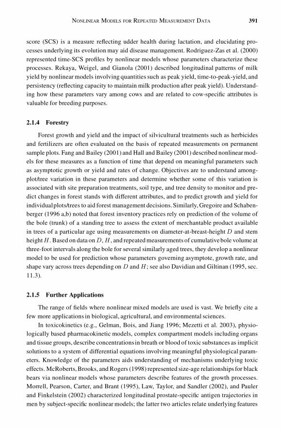
2.1.1 Pharmacokinetics

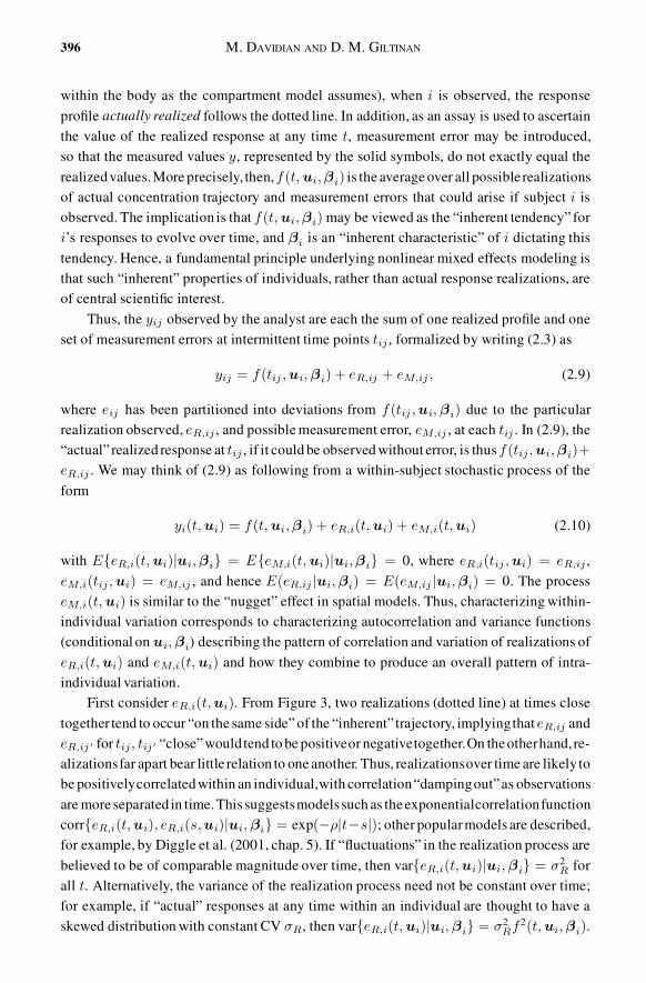
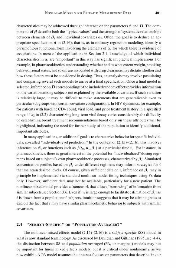
Figure 1 shows data typical of an intensive pharmacokinetic study (Davidian and Gilti-nan 1995, sec. 5.5) carried out early in drug development to gain insight into within-subjectpharmacokinetic processes of absorption, distribution, and elimination governing concen-trations of drug achieved. Twelve subjects were given the same oral dose (mg/kg) of theanti-asthmatic agent theophylline, and blood samples drawn at several times following ad-ministration were assayed for theophylline concentration. As ordinarily observed in thiscontext, the concentration pro�les have a similar shape for all subjects; however, peakconcentration achieved, rise, and decay vary substantially. These differences are believedto be attributable to inter-subject variation in the underlying pharmacokinetic processes,understanding of which is critical for developing dosing guidelines.

To characterize these processes formally, it is routine represent the body by a simplecompartment model (e.g., Sheiner and Ludden 1992). For theophylline,a one-compartmentmodel is standard, and solution of the corresponding differential equations yields

C(t) =Dka

V (ka ¡ Cl=V )

½exp(¡kat) ¡ exp

μ¡Cl

Vt

¶¾; (2.1)

NONLINEAR MODELS FOR REPEATED MEASUREMENT DATA 389

Time (hr)

Th

eoph

yllin

eC

on

c.(m

g/L

)

0 5 10 15 20 25

02

46

81

012

Figure 1. Theophylline concentrations for 12 subjects following a single oral dose.

where C(t) is drug concentration at time t for a single subject following oral dose D att = 0. Here, ka is the fractional rate of absorption describing how drug is absorbed fromthe gut into the bloodstream; V is roughly the volume required to account for all drug inthe body, re�ecting the extent of drug distribution;and Cl is the clearance rate representingthe volume of blood from which drug is eliminated per unit time. Thus, the parameters(ka; V; Cl) in (2.1) summarize the pharmacokinetic processes for a given subject.

More precisely stated, the goal is to determine, based on the observed pro�les, meanor median values of (ka; V; Cl), and how they vary in the population of subjects in orderto design repeated dosing regimens to maintain drug concentrations in a desired range. Ifinter-subject variation in (ka; V; Cl) is large, it may be dif�cult to design an “all-purpose”regimen; however, if some of the variation is associated with subject characteristics such asage or weight, this might be used to develop strategies tailored for certain subgroups.

2.1.2 HIV Dynamics

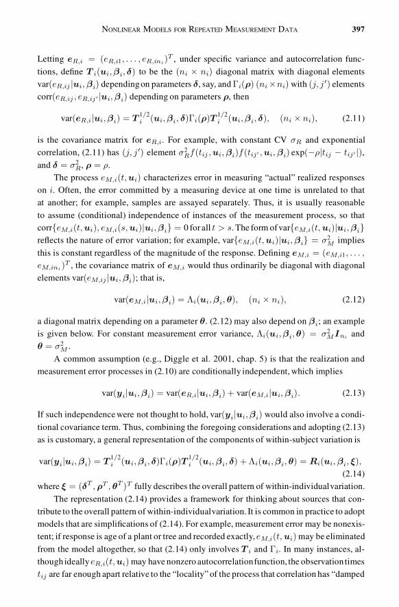
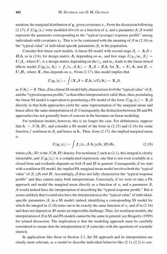
With the advent of assays capable of quantifying the concentration of viral particles inthe blood, monitoring of such “viral load” measurements is now a routine feature of care ofHIV-infected individuals.Figure2 showsviral load-timepro�les for ten participantsin AIDSClinicalTrial Group (ACTG) protocol315(Wu and Ding 1999)followinginitiationof potentantiretroviral therapy. Characterizing mechanisms of virus-immune system interaction thatlead to such patterns of viral decay (and eventual rebound for many subjects) enhancesunderstanding of the progression of HIV disease.


0 20 40 60 80

12

34

56

7

Days

log1

0P

lasm

aR

NA

(cop

ies/

ml)

Figure 2. Viral load pro�les for 10 subjects from the ACTG 315 study. The lower limit of detection of 100 copies/mlis denoted by the dotted line.

Considerable recent interest has focused on representing within-subject mechanismsby a system of differential equations whose parameters characterize rates of production,infection, and death of immune system cells and viral production and clearance (Wu andDing 1999, sec. 2). Under assumptionsdiscussed by these authors, typical models for V (t),the concentration of virus particles at time t following treatment initiation, are of the form

V (t) = P1 exp(¡¶1t) + P2 exp(¡¶2t); (2.2)

where (P1; ¶1; P2; ¶2) describe patterns of viral production and decay. Understanding the“typical” values of these parameters, how they vary among subjects, and whether they areassociated with measures of disease status at initiationof therapy such as baseline viral load(e.g., Notermans et al. 1998)may guideuse of drugs in the anti-HIV arsenal.A complicationis that viral loads below the lower limit of detection of the assay are not quanti�able andare usually coded as equal to the limit (100 copies/ml for ACTG 315).

2.1.3 Dairy Science

In�ammation of the mammary gland in dairy cattle has serious economic implica-tions for the dairy industry (Rodriguez-Zas, Gianola, and Shook 2000). Milk somatic cell


score (SCS) is a measure re�ecting udder health during lactation, and elucidating pro-cesses underlying its evolution may aid disease management. Rodriguez-Zas et al. (2000)represented time-SCS pro�les by nonlinear models whose parameters characterize theseprocesses. Rekaya, Weigel, and Gianola (2001) described longitudinal patterns of milkyield by nonlinear models involving quantities such as peak yield, time-to-peak-yield, andpersistency (re�ecting capacity to maintain milk production after peak yield). Understand-ing how these parameters vary among cows and are related to cow-speci�c attributes isvaluable for breeding purposes.

2.1.4 Forestry

Forest growth and yield and the impact of silvicultural treatments such as herbicidesand fertilizers are often evaluated on the basis of repeated measurements on permanentsample plots. Fang and Bailey (2001) and Hall and Bailey (2001) described nonlinear mod-els for these measures as a function of time that depend on meaningful parameters suchas asymptotic growth or yield and rates of change. Objectives are to understand among-plot/tree variation in these parameters and determine whether some of this variation isassociated with site preparation treatments, soil type, and tree density to monitor and pre-dict changes in forest stands with different attributes, and to predict growth and yield forindividualplots/trees to aid forest management decisions.Similarly, Gregoire and Schaben-berger (1996 a,b) noted that forest inventory practices rely on prediction of the volume ofthe bole (trunk) of a standing tree to assess the extent of merchantable product availablein trees of a particular age using measurements on diameter-at-breast-height D and stemheightH . Based on data on D, H , and repeated measurements of cumulativebole volume atthree-foot intervals along the bole for several similarly aged trees, they develop a nonlinearmodel to be used for prediction whose parameters governing asymptote, growth rate, andshape vary across trees depending on D and H ; see also Davidian and Giltinan (1995, sec.11.3).

2.1.5 Further Applications

The range of �elds where nonlinear mixed models are used is vast. We brie�y cite afew more applications in biological, agricultural, and environmental sciences.

In toxicokinetics (e.g., Gelman, Bois, and Jiang 1996; Mezetti et al. 2003), physio-logically based pharmacokinetic models, complex compartment models including organsand tissue groups, describe concentrationsin breath or blood of toxic substances as implicitsolutions to a system of differential equations involving meaningful physiological param-eters. Knowledge of the parameters aids understanding of mechanisms underlying toxiceffects. McRoberts,Brooks, and Rogers (1998) represented size-age relationships for blackbears via nonlinear models whose parameters describe features of the growth processes.Morrell, Pearson, Carter, and Brant (1995), Law, Taylor, and Sandler (2002), and Paulerand Finkelstein (2002) characterized longitudinal prostate-speci�c antigen trajectories inmen by subject-speci�c nonlinear models; the latter two articles relate underlying features


of the pro�les to cancer recurrence. Muller and Rosner (1997) described patterns of whiteblood cell and granulocyte counts for cancer patients undergoing high-dose chemother-apy by nonlinear models whose parameters characterize important features of the pro�les;knowledge of the relationship of these features to patient characteristics aids evaluation oftoxicity and prediction of hematologic pro�les for future patients. Mikulich, Zerbe, Jones,and Crowley (2003) used nonlinearmixed models in analyses of data on circadian rhythms.Additional applications are found in the literature in �sheries science (Pilling, Kirkwood,and Walker 2002) and plant and soil sciences (Schabenberger and Pierce 2001).

2.1.6 Summary

These situations share several features: (1) repeated observations of a continuous re-sponseon each of several individuals(e.g., subjects,plots,cows) over time or other condition(e.g., intervals along a tree bole); (2) variability in the relationship between response andtime or other condition across individuals; and (3) availability of a scienti�cally relevantmodel characterizingindividualbehavior in terms of meaningfulparameters that vary acrossindividuals and dictate variation in patterns of time-response. Objectives are to understandthe “typical” behavior of the phenomena represented by the parameters; the extent to whichthe parameters, and hence these phenomena, vary across individuals; and whether some ofthe variation is systematically associated with individualattributes. Individual-levelpredic-tion may also be of interest. As we now describe, the nonlinear mixed effects model is anappropriate framework within which to formalize these objectives.

2.2 THE MODEL

2.2.1 Basic Model

We consider a basic version of the model here and in Section 3; extensions are dis-cussed in Section 4. Let yij denote the jth measurement of the response, for example, drugconcentration or milk yield, under condition tij , j = 1; : : : ; ni, and possible additionalconditions ui. For example, for theophylline, tij is the time associated with the jth drugconcentration for subject i following dose ui = Di at time zero. In many applications,tij is time and ui is empty, and we use the word “time” generically below. We write forbrevity xij = (tij ; ui), but note dependence on tij where appropriate. Assume that theremay be a vector of characteristics ai for each individual that do not change with time,for example, age, weight, or diameter-at-breast-height. Letting yi = (yi1; : : : ; yini )T , itis ordinarily assumed that the triplets (yi; ui; ai) are independent across i, re�ecting thebelief that individuals are “unrelated.” The usual nonlinear mixed effects model may thenbe written as a two-stage hierarchy as follows:

Stage 1: Individual-Level Model. yij = f (xij ; ¯i) + eij ; j = 1; : : : ; ni: (2.3)


In (2.3), f is a functiongoverningwithin-individualbehavior,such as (2.1)–(2.2), dependingon a (p £ 1) vector of parameters ¯i speci�c to individual i. For example, in (2.1), ¯i =

(kai; Vi; Cli)T = (�1i; �2i; �3i)

T , where kai, Vi, and Cli are absorption rate, volume, andclearance for subject i. The intra-individualdeviations eij = yij ¡ f (xij ; ¯i) are assumedto satisfy E(eij jui; ¯i) = 0 for all j; we say more about other properties of the eij shortly.

Stage 2: Population Model. ¯i = d(ai; ¯; bi); i = 1; : : : ; m; (2.4)

where d is a p-dimensional function depending on an (r £ 1) vector of �xed parameters, or�xed effects, ¯ and a (k £ 1) vector of random effects bi associated with individual i. Here,(2.4) characterizes how elements of ¯i vary among individuals, due both to systematicassociation with individual attributes in ai and to “unexplained”variation in the populationof individuals,for example, natural, biologicalvariation, represented by bi. The distributionof the bi conditional on ai is usually taken not to depend on ai (i.e., the bi are independentof the ai), with E(bijai) = E(bi) = 0 and var(bijai) = var(bi) = D. Here, D is anunstructured covariancematrix that is the same for all i, and D characterizes the magnitudeof “unexplained” variation in the elements of ¯i and associations among them; a standardsuch assumption is bi ¹ N (0; D). We discuss this assumption further momentarily.

For instance, if ai = (wi; ci)T , where for subject i wi is weight (kg) and ci = 0

if creatinine clearance is μ 50 ml/min, indicating impaired renal function, and ci = 1otherwise, then for a pharmacokinetic study under (2.1), an example of (2.4), with bi =

(b1i; b2i; b3i)T , is

kai = exp(�1 + b1i);

Vi = exp(�2 + �3wi + b2i);

Cli = exp(�4 + �5wi + �6ci + �7wici + b3i): (2.5)

Model (2.5) enforces positivity of the pharmacokinetic parameters for each i. Moreover, ifbi is multivariate normal, kai; Cli; Vi are each lognormally distributed in the population,consistent with the widely acknowledged phenomenon that these parameters have skewedpopulation distributions. Here, the assumption that the distribution of bi given ai does notdepend on ai corresponds to the belief that variation in the parameters “unexplained” bythe systematic relationshipswith wi and ci in (2.5) is the same regardless of weight or renalstatus, similar to standard assumptions in ordinary regression modeling. For example, ifbi ¹ N (0; D), then log Cli is normal with variance D33, and thus Cli is lognormal withcoef�cient of variation (CV) exp(D33)¡1, neitherof which dependson wi; ci. On the otherhand, if this variation is thought to be different, the assumption may be relaxed by takingbijai ¹ N f0; D(ai)g, where now the covariance matrix depends on ai. For example,if the parameters are more variable among subjects with normal renal function, one mayassume D(ai) = D0(1 ¡ ci) + D1ci; so that the covariance matrix depends on ai throughci and equals D0 in the subpopulationof individualswith renal impairment and D1 in thatof healthy subjects.

In (2.5), each element of ¯i is taken to have an associated random effect, re�ecting thebelief that each component varies nonnegligibly in the population, even after systematic


relationships with subject characteristics are taken into account. In some settings, “unex-plained” variation in one component of ¯i may be very small in magnitude relative to thatin others. It is common to approximate this by taking this component to have no associatedrandom effect; for example, in (2.5), specify instead Vi = exp(�2 + �3wi), which attributesall variation in volumes across subjects to differences in weight. Usually, it is biologicallyimplausible for there to be no “unexplained” variation in the features represented by theparameters, so one must recognize that such a speci�cation is adopted mainly to achieveparsimony and numerical stability in �tting rather than to re�ect belief in perfect biologicalconsistency across individuals. Analyses in the literature to determine “whether elementsof ¯i are �xed or random effects” should be interpreted in this spirit.

A common special case of (2.4) is that of a linear relationship between ¯i and �xedand random effects as in usual, empirical statistical linear modeling, that is,

¯i = Ai¯ + Bibi; (2.6)

where Ai is a designmatrix dependingon elementsof ai, and Bi is a designmatrix typicallyinvolving only zeros and ones allowing some elements of ¯i to have no associated randomeffect. For example, consider the linear alternative to (2.5) given by

kai = �1 + b1i; Vi = �2 + �3wi; Cli = �4 + �5wi + �6ci + �7wici + b3i (2.7)

with bi = (b1i; b3i)T , which may be represented as in (2.6) with ¯ = (�1; : : : ; �7)

T , and

Ai =

0B@ 1 0 0 0 0 0 00 1 wi 0 0 0 00 0 0 1 wi ci wici

1CA ; Bi =

0B@ 1 00 00 1

1CA ;

(2.7) takes Vi to vary negligiblyrelative to kai and Cli. Alternatively,if Vi = �2+�3wi+b2i,so including “unexplained”variation in this parameter above and beyond that explained byweight, bi = (b1i; b2i; b3i)

T and Bi = I3, where Iq is a q-dimensional identity matrix.If bi is multivariate normal, a linear speci�cation as in (2.7) may be unrealistic for ap-

plicationswhere populationdistributionsare thought to be skewed, as in pharmacokinetics.Rather than adopt a nonlinear population model as in (2.5), a common alternative tactic isto reparameterize the model f . For example, if (2.1) is represented in terms of parameters(k¤

a; V ¤; Cl¤)T = (logka; logV; logCl)T , then ¯i = (k¤ai; V ¤

i ; Cl¤i )T , and

k¤ai = �1 + b1i;

V ¤i = �2 + �3wi + b2i;

Cl¤i = �4 + �5wi + �6ci + �7wici + b3i (2.8)

is a linear population model in the same spirit as (2.5).In summary, speci�cation of the population model (2.4) is made in accordance with

usual considerations for regression modeling and subject-matter knowledge. Taking Ai =

Ip in (2.6) with ¯ = (�1; : : : ; �p)T assumes E(�`i) = �` for ` = 1; : : : ; p, which may bedone in the case where no individual covariates ai are available or as a part of a model-building exercise; see Section 3.6. If the data arise according to a design involving �xed


t

C(t

)

0 5 10 15 20

02

46

810

12

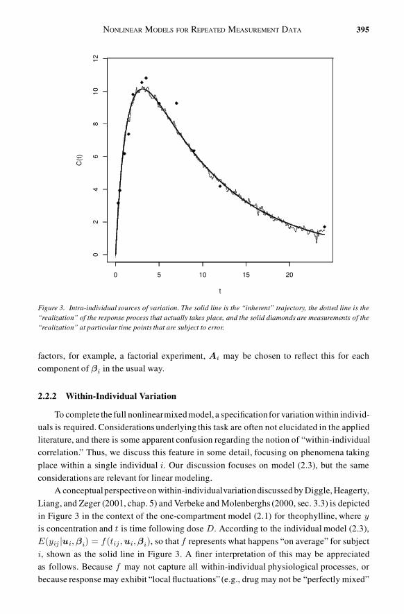
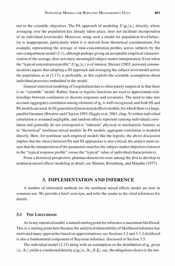
Figure 3. Intra-individual sources of variation. The solid line is the “inherent” trajectory, the dotted line is the“realization” of the response process that actually takes place, and the solid diamonds are measurements of the“realization” at particular time points that are subject to error.

factors, for example, a factorial experiment, Ai may be chosen to re�ect this for eachcomponent of ¯i in the usual way.

2.2.2 Within-Individual Variation

To complete the full nonlinearmixedmodel, a speci�cationfor variationwithin individ-uals is required. Considerations underlying this task are often not elucidated in the appliedliterature, and there is some apparent confusion regarding the notion of “within-individualcorrelation.” Thus, we discuss this feature in some detail, focusing on phenomena takingplace within a single individual i. Our discussion focuses on model (2.3), but the sameconsiderations are relevant for linear modeling.

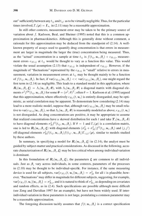
A conceptualperspectiveon within-individualvariationdiscussed by Diggle, Heagerty,Liang, and Zeger (2001, chap. 5) and Verbeke and Molenberghs (2000, sec. 3.3) is depictedin Figure 3 in the context of the one-compartment model (2.1) for theophylline, where y

is concentration and t is time following dose D. According to the individual model (2.3),E(yij jui; ¯i) = f (tij ; ui; ¯i), so that f represents what happens “on average” for subjecti, shown as the solid line in Figure 3. A �ner interpretation of this may be appreciatedas follows. Because f may not capture all within-individual physiological processes, orbecause response may exhibit “local �uctuations” (e.g., drug may not be “perfectly mixed”


within the body as the compartment model assumes), when i is observed, the responsepro�le actually realized follows the dotted line. In addition, as an assay is used to ascertainthe value of the realized response at any time t, measurement error may be introduced,so that the measured values y, represented by the solid symbols, do not exactly equal therealizedvalues.More precisely, then,f (t; ui; ¯i) is the averageover all possible realizationsof actual concentration trajectory and measurement errors that could arise if subject i isobserved. The implication is that f (t; ui; ¯i) may be viewed as the “inherent tendency” fori’s responses to evolve over time, and ¯i is an “inherent characteristic” of i dictating thistendency. Hence, a fundamental principle underlying nonlinear mixed effects modeling isthat such “inherent” properties of individuals, rather than actual response realizations, areof central scienti�c interest.

Thus, the yij observed by the analyst are each the sum of one realized pro�le and oneset of measurement errors at intermittent time points tij , formalized by writing (2.3) as

yij = f (tij ; ui; ¯i) + eR;ij + eM;ij ; (2.9)

where eij has been partitioned into deviations from f (tij ; ui; ¯i) due to the particularrealization observed, eR;ij , and possible measurement error, eM;ij , at each tij . In (2.9), the“actual” realized response at tij , if it could be observed without error, is thusf (tij ; ui; ¯i)+

eR;ij . We may think of (2.9) as following from a within-subject stochastic process of theform

yi(t; ui) = f (t; ui; ¯i) + eR;i(t; ui) + eM;i(t; ui) (2.10)

with EfeR;i(t; ui)jui; ¯ig = EfeM;i(t; ui)jui; ¯ig = 0, where eR;i(tij ; ui) = eR;ij ,eM;i(tij ; ui) = eM;ij , and hence E(eR;ij jui; ¯i) = E(eM;ij jui; ¯i) = 0. The processeM;i(t; ui) is similar to the “nugget” effect in spatial models. Thus, characterizing within-individual variation corresponds to characterizing autocorrelation and variance functions(conditional on ui; ¯i) describing the pattern of correlation and variation of realizations ofeR;i(t; ui) and eM;i(t; ui) and how they combine to produce an overall pattern of intra-individual variation.

First consider eR;i(t; ui). From Figure 3, two realizations (dotted line) at times closetogether tend to occur “on the same side” of the “inherent” trajectory, implyingthateR;ij andeR;ij 0 for tij ; tij 0 “close”would tend to be positiveor negativetogether.On theotherhand,re-alizationsfar apart bear little relation to one another. Thus, realizationsover time are likely tobe positivelycorrelatedwithin an individual,with correlation“dampingout”as observationsare more separated in time.This suggestsmodelssuch as theexponentialcorrelationfunctioncorrfeR;i(t; ui); eR;i(s; ui)jui; ¯ig = exp(¡�jt¡sj); other popularmodels are described,for example, by Diggle et al. (2001, chap. 5). If “�uctuations” in the realization process arebelieved to be of comparable magnitude over time, then varfeR;i(t; ui)jui; ¯ig = ¼2

R forall t. Alternatively, the variance of the realization process need not be constant over time;for example, if “actual” responses at any time within an individual are thought to have askewed distribution with constant CV ¼R, then varfeR;i(t; ui)jui; ¯ig = ¼2

Rf2(t; ui; ¯i).


Letting eR;i = (eR;i1; : : : ; eR;ini )T , under speci�c variance and autocorrelation func-

tions, de�ne T i(ui; ¯i; ±) to be the (ni £ ni) diagonal matrix with diagonal elementsvar(eR;ij jui; ¯i) dependingon parameters ±, say, and ¡i(½) (ni £ni) with (j; j 0) elementscorr(eR;ij ; eR;ij 0 jui; ¯i) depending on parameters ½, then

var(eR;ijui; ¯i) = T1=2i (ui; ¯i; ±)¡i(½)T

1=2i (ui; ¯i; ±); (ni £ ni); (2.11)

is the covariance matrix for eR;i. For example, with constant CV ¼R and exponentialcorrelation, (2.11) has (j; j 0) element ¼2

Rf (tij ; ui; ¯i)f (tij 0 ; ui; ¯i) exp(¡�jtij ¡ tij 0 j),and ± = ¼2

R, ½ = �.The process eM;i(t; ui) characterizes error in measuring “actual” realized responses

on i. Often, the error committed by a measuring device at one time is unrelated to thatat another; for example, samples are assayed separately. Thus, it is usually reasonableto assume (conditional) independence of instances of the measurement process, so thatcorrfeM;i(t; ui); eM;i(s; ui)jui; ¯ig = 0 for all t > s. The form ofvarfeM;i(t; ui)jui; ¯igre�ects the nature of error variation; for example, varfeM;i(t; ui)jui; ¯ig = ¼2

M impliesthis is constant regardless of the magnitude of the response. De�ning eM;i = (eM;i1; : : : ;

eM;ini )T , the covariance matrix of eM;i would thus ordinarily be diagonal with diagonalelements var(eM;ij jui; ¯i); that is,

var(eM;ijui; ¯i) = ¤i(ui; ¯i; μ); (ni £ ni); (2.12)

a diagonal matrix depending on a parameter μ. (2.12) may also depend on ¯i; an exampleis given below. For constant measurement error variance, ¤i(ui; ¯i; μ) = ¼2

M Ini andμ = ¼2

M .A common assumption (e.g., Diggle et al. 2001, chap. 5) is that the realization and

measurement error processes in (2.10) are conditionally independent, which implies

var(yijui; ¯i) = var(eR;ijui; ¯i) + var(eM;ijui; ¯i): (2.13)

If such independencewere not thought to hold, var(yijui; ¯i) would also involve a condi-tional covariance term. Thus, combining the foregoing considerations and adopting (2.13)as is customary, a general representation of the components of within-subject variation is

var(yijui; ¯i) = T1=2i (ui; ¯i; ±)¡i(½)T

1=2i (ui; ¯i; ±) + ¤i(ui; ¯i; μ) = Ri(ui; ¯i; �);

(2.14)where � = (±T ; ½T ; μT )T fully describes the overall pattern of within-individualvariation.

The representation (2.14) provides a framework for thinking about sources that con-tribute to the overall pattern of within-individualvariation. It is common in practice to adoptmodels that are simpli�cations of (2.14). For example, measurement error may be nonexis-tent; if response is age of a plant or tree and recorded exactly,eM;i(t; ui) may be eliminatedfrom the model altogether, so that (2.14) only involves T i and ¡i. In many instances, al-though ideallyeR;i(t; ui) may have nonzero autocorrelationfunction, the observation timestij are far enough apart relative to the “locality” of the process that correlation has “damped


out” suf�cientlybetween any tij and tij 0 as to be virtuallynegligible.Thus, for the particulartimes involved, ¡i(½) = Ini in (2.11) may be a reasonable approximation.

In still other contexts, measurement error may be taken to be the primary source ofvariation about f . Karlsson, Beal, and Sheiner (1995) noted that this is a common ap-proximation in pharmacokinetics. Although this is generally done without comment, arationale for this approximation may be deduced from the standpoint of (2.14). A well-known property of assays used to quantify drug concentration is that errors in measure-ment are larger in magnitude the larger the (true) concentration being measured. Thus,as the “actual” concentration in a sample at time tij is f (tij ; ui; ¯i) + eR;ij , measure-ment errors eM;ij at tij would be thought to vary as a function this value. This wouldviolate the usual assumption (2.13) that eM;ij is independent of eR;ij . However, if themagnitude of “�uctuations” represented by the eR;ij is “small” relative to errors in mea-surement, variation in measurement errors at tij may be thought mainly to be a functionof f (tij ; ui; ¯i). In fact, if var(eR;ij jui; ¯i) << var(eM;ij jui; ¯i), one might regard the�rst term in (2.14) as negligible. This leads to a standard model in this application, whereRi(ui; ¯i; �) = ¤i(ui; ¯i; μ), with ¤i(ui; ¯i; μ) a diagonal matrix with diagonal ele-ments ¼2f 2�(tij ; ui; ¯i) for some μ = (¼2; �)T ; often � = 1. Karlsson et al. (1995) arguedthat this approximation, where effectively eR;i(t; ui) is entirely disregarded, may be opti-mistic, as serial correlation may be apparent. To demonstrate how considering (2.14) maylead to a more realistic model, suppose that, although var(eR;ij jui; ¯i) may be small rela-tive to var(eM;ij jui; ¯i), so that ¤i(ui; ¯i; μ) is reasonably modeled as above, eR;i(t; ui)

is not disregarded. As drug concentrations are positive, it may be appropriate to assumethat realized concentrations have a skewed distribution for each t and take T i(ui; ¯i; ±)

to have diagonal elements ¼2Rf 2(tij ; ui; ¯i). If � = 1 and ¡i(½) is a correlation matrix,

one is led to Ri(ui; ¯i; �) with diagonal elements (¼2R + ¼2

M )f 2(tij ; ui; ¯i) and (j; j 0)off-diagonal elements ¼2

Rf (tij ; ui; ¯i)f (tij 0 ; ui; ¯i)¡i;jj 0 (½), similar to models studiedby these authors.

In summary, in specifying a model for Ri(ui; ¯i; �) in (2.14), the analyst must beguided by subject-matter and practical considerations. As discussed in the following, accu-rate characterization of Ri(ui; ¯i; �) may be less critical when among-individualvariationis dominant.

In this formulation of Ri(ui; ¯i; �), the parameters � are common to all individ-uals. Just as ¯i vary across individuals, in some contexts, parameters of the processesin (2.10) may be thought to be individual-speci�c. For instance, if the same measuringdevice is used for all subjects, varfeM;i(t; ui)jui; ¯i) = ¼2

M for all i is plausible; how-ever, “�uctuations”may differ in magnitude for different subjects, suggesting, for example,varfeR;i(t; ui)jui; ¯ig = ¼2

R;i, and it is natural to think of ¼2R;i as dependingon covariates

and random effects, as in (2.4). Such speci�cations are possible although more dif�cult(see Zeng and Davidian 1997 for an example), but have not been widely used. If inter-individual variation in these parameters is not large, postulating a common parameter maybe a reasonable approximation.

The foregoing discussion tacitly assumes that f (t; ui; ¯i) is a correct speci�cation


of “inherent” individual behavior, with actual realizations �uctuating about f (t; ui; ¯i).Thus, deviations arising from eR;i(t; ui) in (2.10) are regarded as part of within-individualvariation and hence not of direct interest. An alternative view is that a component of thesedeviations is due to misspeci�cation of f (t; ui; ¯i). For example, in pharmacokinetics,compartment models used to characterize the body are admittedly simplistic, so systematicdeviations from f (t; ui; ¯i) due to their failure to capture the true “inherent” trajectoryare possible. If, for example, other “local” variation is negligible, the process eR;i(t; ui)

in (2.10) in fact re�ects entirely such misspeci�cation, and the true, “inherent trajectory”would be f(t; ui; ¯i) + eR;i(t; ui), so that f (t; ui; ¯i) alone is a biased representationof the true trajectory. Here, eR;i(t; ui) should be regarded as part of the “signal” ratherthan as “noise.” More generally, under misspeci�cation, part of eR;i(t; ui) is due to suchsystematic deviations and part is due to “�uctuations,” but without knowledge of the ex-act nature of misspeci�cation, distinguishing bias from within-individual variation makeswithin-individualcovariance modeling a nearly impossible challenge. In the particular con-text of nonlinear mixed effects models, there are also obvious implications for the meaningand relevance of ¯i under a misspeci�ed model. We do not pursue this further; however,it is vital to recognize that published applications of nonlinear mixed effects models arealmost always predicated on correctness of f (t; ui; ¯i).

2.2.3 Summary

We are now in a position to summarize the basic nonlinear mixed effects model. Letf i(ui; ¯i) = ff (xi1; ¯i); : : : ; f (xini ; ¯i)gT , and let zi = (uT

i ; aTi )T summarize all

covariateinformationon subjecti. Then,we maywrite themodel in (2.3) and (2.4) succinctlyas

Stage 1: Individual-Level Model.

E(yijzi; bi) = f i(ui; ¯i) = f i(zi; ¯; bi);

var(yijzi; bi) = Ri(ui; ¯i; �) = Ri(zi; ¯; bi; �): (2.15)

Stage 2: Population Model. ¯i = d(ai; ¯; bi); bi ¹ (0; D): (2.16)

In (2.15), dependenceof f i and Ri on thecovariatesai and �xed and randomeffects through¯i is emphasized. This model represents individual behavior conditional on ¯i and henceon bi, the random component in (2.16). In (2.16), we assume that the distribution of bijai

does not depend on ai, so that all bi have common distributionwith mean 0 and covariancematrix D. We adopt this assumption in the sequel, as it is routine in the literature, but themethodswe discussmay be extended if it is relaxed in the mannerdescribed in Section 2.2.1.

2.2.4 “Within-Individual Correlation”

The nonlinear mixed model (2.15)–(2.16) implies a model for the marginal mean andcovariance matrix of yi given all covariates zi; that is, averaged across the population.


Letting Fb(bi) denote the cumulative distribution function of bi, we have

E(yijzi) =

Zf i(zi; ¯; bi) dFb(bi);

var(yijzi) = EfRi(zi; ¯; bi; �)jzig + varff i(zi; ¯; bi)jzig; (2.17)

where expectationand variance are with respect to the distributionof bi. In (2.17), E(yijzi)

characterizes the “typical” response pro�le among individuals with covariates zi. In theliterature,var(yijzi) is often referred to as the “within-subjectcovariancematrix;”however,this is misleading. In particular, var(yijzi) involves two terms: EfRi(zi; ¯; bi; �)jzig,which averages realization and measurement variation that occur within individuals acrossindividualshaving covariates zi; and varff i(zi; ¯; bi)jzig, which describes how “inherenttrajectories” vary among individuals sharing the same zi. Note EfRi(zi; ¯; bi; �)jzigis a diagonal matrix only if ¡i(½) in (2.14), re�ecting correlation due to within-individualrealizations, is an identity matrix. However, varff i(zi; ¯; bi)jzig has nonzero off-diagonalelements in general due to commondependenceof all elementsof f i on bi. Thus, correlationat the marginal level is always expected due to variation among individuals, while there iscorrelation from within-individualsources only if serial associationsamong intra-individualrealizations are nonnegligible. In general, then, both terms contribute to the overall patternof correlation among responses on the same individual represented in var(yijzi).

Thus, the terms “within-individualcovariance” and “within-individualcorrelation” arebetter reserved to refer to phenomena associated with the realization process eR;i(t; ui).We prefer “aggregate correlation” to denote the overall population-averaged pattern ofcorrelation arising from both sources. It is important to recognize that within-individualvarianceand correlationare relevanteven if scopeof inference is limited to a given individualonly.

As notedby Diggle et al. (2001, chap. 5) and Verbeke and Molenberghs(2000, sec. 3.3),in many applications, the effect of within-individual serial correlation re�ected in the �rstterm of var(yijzi) is dominated by that from among-individual variation in varff i(zi; ¯;

bi)jzig. This explains why many published applications of nonlinear mixed models adoptsimple, diagonalmodels for Ri(ui; ¯i; �) that emphasize measurement error. Davidian andGiltinan(1995, secs. 5.2.4and 11.3), suggestedthat, here, how one modelswithin-individualcorrelation, or, in fact, whether one improperly disregards it, may have inconsequentialeffects on inference. It is the responsibility of the data analyst to evaluate critically therationale for and consequences of adopting a simpli�ed model in a particular application.

2.3 INFERENTIAL OBJECTIVES

We now state more precisely routine objectives of analyses based on the nonlinearmixed effects model, discussed at the end of Section 2.1. Implementation is discussed inSection 3.

Understanding the “typical” values of the parameters in f , how they vary across indi-viduals in the population, and whether some of this variation is associated with individual


characteristics may be addressed through inference on the parameters ¯ and D. The com-ponents of ¯ describe both the “typical values” and the strength of systematic relationshipsbetween elements of ¯i and individual covariates ai. Often, the goal is to deduce an ap-propriate speci�cation d in (2.16); that is, as in ordinary regression modeling, identify aparsimonious functional form involving the elements of ai for which there is evidence ofassociations. In most of the applications in Section 2.1, knowledge of which individualcharacteristics in ai are “important” in this way has signi�cant practical implications. Forexample, in pharmacokinetics, understanding whether and to what extent weight, smokingbehavior, renal status, and so on. are associatedwith drug clearance may dictatewhether andhow these factors must be considered in dosing. Thus, an analysis may involve postulatingand comparing several such models to arrive at a �nal speci�cation. Once a �nal model isselected, inferenceon D correspondingto the includedrandom effects provides informationon the variation among subjects not explained by the available covariates. If such variationis relatively large, it may be dif�cult to make statements that are generalizable even toparticular subgroups with certain covariate con�gurations. In HIV dynamics, for example,for patients with baseline CD4 count, viral load, and prior treatment history in a speci�edrange, if ¶2 in (2.2) characterizing long-term viral decay varies considerably, the dif�cultyof establishing broad treatment recommendations based only on these attributes will behighlighted, indicating the need for further study of the population to identify additional,important attributes.

In many applications,an additionalgoal is to characterize behavior for speci�c individ-uals, so-called “individual-level prediction.” In the context of (2.15)–(2.16), this involvesinference on ¯i or functions such as f (t0; ui; ¯i) at a particular time t0. For instance, inpharmacokinetics, there is great interest in the potential for “individualized” dosing regi-mens based on subject i’s own pharmacokinetic processes, characterized by ¯i. Simulatedconcentration pro�les based on ¯i under different regimens may inform strategies for i

that maintain desired levels. Of course, given suf�cient data on i, inference on ¯i may inprinciple be implemented via standard nonlinear model-�tting techniques using i’s dataonly. However, suf�cient data may not be available, particularly for a new patient. Thenonlinear mixed model provides a framework that allows “borrowing” of information fromsimilar subjects; see Section 3.6. Even if ni is large enough to facilitate estimation of ¯i, asi is drawn from a population of subjects, intuition suggests that it may be advantageous toexploit the fact that i may have similar pharmacokinetic behavior to subjects with similarcovariates.

2.4 ‘‘SUBJECT-SPECIFIC’’ OR ‘‘POPULATION-AVERAGED?’’

The nonlinear mixed effects model (2.15)–(2.16) is a subject-speci�c (SS) model inwhat is now standard terminology. As discussed by Davidian and Giltinan (1995, sec. 4.4),the distinction between SS and population averaged (PA, or marginal) models may notbe important for linear mixed effects models, but it is critical under nonlinearity, as wenow exhibit. A PA model assumes that interest focuses on parameters that describe, in our


notation, the marginal distribution of yi given covariates zi. From the discussion following(2.17), if E(yijzi) were modeled directly as a function of zi and a parameter ¯, ¯ wouldrepresent the parameter corresponding to the “typical (average) response pro�le” amongindividuals with covariates zi. This is to be contrasted with the meaning of ¯ in (2.16) asthe “typical value” of individual-speci�c parameters ¯i in the population.

Consider �rst linear such models. A linear SS model with second stage ¯i = Ai¯ +

Bibi as in (2.6), for design matrix Ai depending on ai, and �rst stage E(yij jui; ¯i) =

U i¯i, where U i is a design matrix depending on the tij and ui, leads to the linear mixedeffects model E(yijzi; bi) = f i(zi; ¯; bi) = X i¯ + Zibi for X i = U iAi and Zi =

U iBi, where X i thus depends on zi. From (2.17), this model implies that

E(yijzi) =

Z(X i¯ + Zibi) dFb(bi) = Xi¯;

as E(bi) = 0. Thus, ¯ in a linearSS model fully characterizes both the “typical value” of ¯i

and the “typicalresponsepro�le,” so that either interpretationis valid.Here, then,postulatingthe linear SS model is equivalent to postulating a PA model of the form E(yijzi) = X i¯

directly in that both approaches yield the same representation of the marginal mean andhence allow the same interpretation of ¯. Consequently, the distinction between SS and PAapproaches has not generally been of concern in the literature on linear modeling.

For nonlinear models, however, this is no longer the case. For de�niteness, supposethat bi ¹ N (0; D), and consider a SS model of the form in (2.15) and (2.16) for somefunction f nonlinear in ¯i and hence in bi. Then, from (2.17), the implied marginal meanis

E(yijzi) =

Zf i(zi; ¯; bi)p(bi; D)dbi; (2.18)

where p(bi; D) is the N (0; D) density.For nonlinearf such as (2.1), this integral is clearlyintractable, and E(yijzi) is a complicated expression, one that is not even available in aclosed form and evidently depends on both ¯ and D in general. Consequently, if we startwith a nonlinear SS model, the implied PA marginal mean model involves both the “typicalvalue” of ¯i (¯) and D. Accordingly, ¯ does not fully characterize the “typical responsepro�le” and thus cannot enjoy both interpretations. Conversely, if we were to take a PAapproach and model the marginal mean directly as a function of zi and a parameter ¯,¯ would indeed have the interpretation of describing the “typical response pro�le.” But itseems unlikely that it could also have the interpretationas the “typical value” of individual-speci�c parameters ¯i in a SS model; indeed, identifying a corresponding SS model forwhich the integral in (2.18) turns out to be exactly the same function of zi and ¯ in (2.16)and does not depend on D seems an impossible challenge. Thus, for nonlinear models, theinterpretationof ¯ in SS and PA models cannot be the same in general; see Heagerty (1999)for related discussion. The implication is that the modeling approach must be carefullyconsidered to ensure that the interpretation of ¯ coincides with the questions of scienti�cinterest.

In applications like those in Section 2.1, the SS approach and its interpretation areclearly more relevant, as a model to describe individual behavior like (2.1)–(2.2) is cen-


tral to the scienti�c objectives. The PA approach of modeling E(yijzi) directly, whereaveraging over the population has already taken place, does not facilitate incorporationof an individual-level model. Moreover, using such a model for population-level behav-ior is inappropriate, particularly when it is derived from theoretical considerations. Forexample, representing the average of time-concentration pro�les across subjects by theone-compartment model (2.1), although perhaps giving an acceptable empirical character-ization of the average, does not enjoy meaningful subject-matter interpretation. Even whenthe “typical concentrationpro�le” E(yijzi) is of interest, Sheiner (2003, personal commu-nication) argues that adopting a SS approach and averaging the subject-level model acrossthe population, as in (2.17), is preferable, as this exploits the scienti�c assumptions aboutindividual processes embedded in the model.

General statistical modeling of longitudinaldata is often purely empirical in that thereis no “scienti�c” model. Rather, linear or logistic functions are used to approximate rela-tionships between continuous or discrete responses and covariates. The need to take intoaccount (aggregate) correlation among elements of yi is well-recognized, and both SS andPA models are used. In SS generalizedlinearmixedeffects models, for which there is a large,parallel literature (Breslow and Clayton 1993;Diggle et al. 2001, chap. 9) within-individualcorrelation is assumed negligible, and random effects represent (among-individual) corre-lation and generally do not correspond to “inherent” physical or mechanistic features asin “theoretical” nonlinear mixed models. In PA models, aggregate correlation is modeleddirectly. Here, for nonlinear such empirical models like the logistic, the above discussionimplies that the choice between PA and SS approaches is also critical; the analyst must en-sure that the interpretationof the parameters matches the subject-matter objectives (interestin the “typical response pro�le” versus the “typical” value of individual characteristics).

From a historical perspective, pharmacokineticists were among the �rst to develop innonlinear mixed effects modeling in detail; see Sheiner, Rosenberg, and Marathe (1977).

3. IMPLEMENTATION AND INFERENCE

A number of inferential methods for the nonlinear mixed effects model are now incommon use. We provide a brief overview, and refer the reader to the cited references fordetails.

3.1 THE LIKELIHOOD

As in any statisticalmodel, a natural startingpoint for inference is maximumlikelihood.This is a starting point here because the analytical intractability of likelihood inference hasmotivated many approaches based on approximations; see Sections 3.2 and 3.3. Likelihoodis also a fundamental component of Bayesian inference, discussed in Section 3.5.

The individual model (2.15) along with an assumption on the distribution of yi given(zi; bi) yields a conditionaldensity p(yijzi; bi; ¯; �), say; the ubiquitouschoice is the nor-


mal. Under the popular (although not always relevant) assumption that Ri(zi; ¯; bi; �) isdiagonal, the density may be written as the product of m contributions p(yij jzi; bi; ¯; �).Under this condition, the lognormal has also been used. At Stage 2, (2.16), adopting in-dependence of bi and ai, one assumes a k-variate density p(bi; D) for bi. As with othermixed models, normality is standard. With these speci�cations, the joint density of (yi; bi)

given zi is

p(yi; bijzi; ; ¯; �; D) = p(yijzi; bi; ¯; �)p(bi; D): (3.1)

(If the distributionof bi given ai is taken to depend on ai, one would substitute for p(bi; D)

in (3.1) the assumed k-variate density p(bijai), which may depend on different parametersfor different values of ai.) A likelihood for ¯; �; D may be based on the joint density ofthe observed data y1; : : : ; ym given zi,

mYi = 1

Zp(yi; bijzi; ; ¯; �; D) dbi =

mYi = 1

Zp(yijzi; bi; ¯; �)p(bi; D) dbi (3.2)

by independence across i. Nonlinearity means that the m k-dimensional integrations in(3.2) generally cannot be done in a closed form; thus, iterative algorithms to maximize(3.2) in ¯; �; D require a way to handle these integrals. Although numerical techniquesfor evaluation of an integral are available, these can be computationally expensive whenperformed at each internal iteration of the algorithm. Hence, many approaches to �tting(2.15)–(2.16) are instead predicated on analytical approximations.

3.2 METHODS BASED ON INDIVIDUAL ESTIMATES

If the ni are suf�ciently large, an intuitive approach is to “summarize” the responsesyi for each i through individual-speci�c estimates b

i and then use these as the basis forinference on ¯ and D. In particular, viewing the conditionalmoments in (2.15) as functionsof ¯i, that is, E(yijui; ¯i) = f (xij ; ¯i), var(yijui; ¯i) = Ri(ui; ¯i; �), �t the modelspeci�ed by these moments for each individual. If Ri(ui; ¯i; �) is a matrix of the form¼2Ini , as in ordinary regression where the yij are assumed (conditionally) independent,standard nonlinear OLS may be used. More generally, methods incorporating estimation ofwithin-individualvariance and correlation parameters � are needed so that intra-individualvariation is taken into appropriate account, as described by Davidian and Giltinan (1993;1995, sec. 5.2).

Usual large-sample theory implies that the individualestimators bi are asymptotically

normal. Each individual is treated separately, so the theory may be viewed as applyingconditionallyon ¯i for each i, yielding b

ijui; ¯i¢¹ N (¯i; C i). Becauseof the nonlinearity

of f in ¯i, C i depends on ¯i in general, so Ci is replaced by bC i in practice, where bi

is substituted. To see how this is exploited for inference on ¯ and D, consider the linearsecond-stagemodel (2.6); the same developmentsapply to any generald in (2.16) (Davidianand Giltinan 1995, sec. 5.3.4). The asymptotic result may be expressed alternatively asb

i º ¯i + e¤i = Ai¯ + Bibi + e¤

i ; e¤i jzi

¢¹ N (0; bC i); bi ¹ N (0; D); (3.3)


where bCi is treated as known for each i, so that the e¤i do not depend on bi. This has

the form of a linear mixed effects model with known “error” covariance matrix bC i, whichsuggests using standard techniques for �tting such models to estimate ¯ and D. Steimer,Mallet, Golmard, and Boisvieux (1984) proposed use of the EM algorithm; the algorithmwas given by Davidian and Giltinan (1995, sec. 5.3.2) in the case k = p and Bi = Ip.Alternatively, it is possible to use linear mixed model software such as SAS proc mixed

(Littell, Milliken, Stroup, and Wol�nger 1996) or the S-Plus/R function lme() (Pinheiroand Bates 2000) to �t (3.3). Because bCi is known and different for each i, and the softwaredefault is to assume var(e¤

i jzi) = ¼2eIp, say, this is simpli�ed by “preprocessing” as

follows. If bC¡1=2i is the Cholesky decompositionof bC¡1

i ; that is, an upper triangularmatrix

satisfying bC¡1=2 T

ibC¡1=2

i = bC¡1i , then bC¡1=2

ibCi

bC¡1=2 T

i = Ip, so that bC¡1=2i e¤

i has

identity covariance matrix. Premultiplying (3.3) by bC¡1=2i yields the “new” linear mixed

model

bC¡1=2i

bi º

μ bC¡1=2i Ai

¶¯ +

μ bC¡1=2i Bi

¶bi + ²i; ²i ¹ N (0; Ip): (3.4)

Fitting (3.4) to the “data” bC¡1=2i

bi with “design matrices” bC¡1=2

i Ai and bC¡1=2i Bi and

the constraint ¼2e = 1 is then straightforward. For either this or the EM algorithm, valid

approximate standard errors are obtained by treating (3.3) as exact.A practical drawback of these methods is that no general-purpose software is available.

S-Plus/R programs implementing both approaches that require some intervention by theuser are available at http://www.stat.ncsu.edu/¹st762 info/.

If the bi are viewed roughly as conditional “suf�cient statistics” for the ¯i, this ap-

proach may be thought of as approximating (3.2) with a change of variables to ¯i byreplacing p(yijzi; bi; ¯; �) by p(b

ijui; ¯i; ¯; �). In point of fact, as the asymptotic resultis not predicated on normality of yijui; ¯i, and because the estimating equations for ¯; D

solved by normal-based linear mixed model software lead to consistent estimators even ifnormality does not hold, this approach does not require normality to achievevalid inference.However, the ni must be large enough for the asymptotic approximation to be justi�ed.

3.3 METHODS BASED ON APPROXIMATION OF THE LIKELIHOOD

This last point is critical when the ni are not large. For example, in populationpharma-cokinetics, sparse, haphazard drug concentrationsover intervals of repeated dosing are col-lected on a large number of subjects along with numerous covariates ai. Although this pro-vides rich information for buildingpopulationmodels d, there are insuf�cient data to �t thepharmacokinetic model f to any one subject (nor to assess its suitability). Implementationof (3.2) in principle imposes no requirements on the magnitudeof the ni. Thus, an attractivetactic is instead to approximate (3.2) in a way that avoids intractable integration. In partic-ular, for each i, an approximation to p(yijzi; ¯; �; D) =

Rp(yijzi; bi; ¯; �)p(bi; D) dbi

is obtained.


3.3.1 First Order Methods

An approach usually attributed to Beal and Sheiner (1982) is motivated by letting R1=2i

be the Cholesky decomposition of Ri and writing (2.15)–(2.16) as

yi = f i(zi; ¯; bi) + R1=2i (zi; ¯; bi; �)²i; ²ijzi; bi ¹ (0; Ini ): (3.5)

As nonlinearity in bi causes the dif�culty for integration in (3.2), it is natural to considera linear approximation. A Taylor series of (3.5) about bi = 0 to linear terms, disregardingthe term involving bi²i as “small” and letting Zi(zi; ¯; b¤) = @=@biff i(zi; ¯; bi)gjbi = b¤

leads to

yi º f i(zi; ¯; 0) + Zi(zi; ¯; 0)bi + R1=2i (zi; ¯; 0; �)²i; (3.6)

E(yijzi) º f i(zi; ¯; 0);

var(yijzi) º Zi(zi; ¯; 0)DZTi (zi; ¯; 0) + Ri(zi; ¯; 0; �): (3.7)

When p(yijzi; bi; ¯; �) in (3.2) is a normal density, (3.6) amounts to approximating itby another normal density whose mean and covariance matrix are linear in and free of bi,respectively. If p(bi; D) is also normal, the integral is analyticallycalculableanalogous to alinear mixed model and yields a ni-variate normal density p(yijzi; ¯; �; D) for each i withmean and covariance matrix (3.7). This suggests the proposal of Beal and Sheiner (1982)to estimate ¯; �; D by jointly maximizing

Qmi = 1 p(yijzi; ¯; �; D), which is equivalent to

maximum likelihood under the assumption the marginal distribution yijzi is normal withmoments (3.7). The advantage is that this “approximate likelihood” is available in a closedform. Standard errors are obtainedfrom the informationmatrix assuming the approximationis exact.

This approach is known as the fo (�rst-order) method in the packagenonmem (Boeck-mann, Sheiner, and Beal 1992, http://www.globomax.net/products/nonmem.cfm) favoredby pharmacokineticists. It is also available in SAS proc nlmixed (SAS Institute 1999)via the method=firo option. As (3.7) de�nes an approximate marginal mean and co-variance matrix for yi given zi, an alternative approach is to estimate ¯; �; D by solvinggeneralized estimating equations (GEEs) (Diggle et al. 2001, chap. 8). Here, the mean isnot of the “generalized linear model” type and the covariance matrix is not a “working”model but rather an approximation to the true structure dictated by the nonlinear mixedmodel; however, the GEE approach is broadly applicable to any marginal moment model.Implementation is available in the SAS nlinmix macro (Littell et al. 1996, chap. 12) withthe expand=zero option. The SAS nlinmix macro and proc nlmixed are distinctpieces of software. nlinmix implements only the �rst order approximate marginal mo-ment model (3.7) using the GEE approach and a related �rst order conditional method,discussed momentarily. In contrast, in addition to implementing (3.7) via the normal like-lihood method above, nlmixed offers several, different alternative approaches to “exact”likelihood inference, described shortly.


Vonesh and Chinchilli (1997, chaps. 8 and 9) and Davidian and Giltinan (1995, sec.6.2.4) described the connections between GEEs and the approximate methods discussedin this section. Brie�y, because the approximation to var(yijzi) in (3.7) depends on ¯,maximizing the approximate normal likelihood corresponds to what has been called a“GEE2” method, which takes full account of this dependence.The ordinary GEE approachnoted above is an example of “GEE1;” here, the dependence of var(yijzi) on ¯ only playsa role in the formation of “weighting matrices” for each data vector yi.

Vonesh and Carter (1992) and Davidian and Giltinan (1995, sec. 6.2.3) discussed fur-ther, related methods. An obvious drawback of all �rst order methods is that the approxi-mation may be poor, as they essentially replace E(yijzi) =

Rf (zi; ¯; bi)p(bi; D) dbi by

f (zi; ¯; 0). This suggests that more re�ned approximation would be desirable.

3.3.2 First Order Conditional Methods

As p(yijzi; bi; ¯; �) and p(bi; D) are ordinarily normal densities, a natural way toapproximate integrals like those in (3.2) is to exploit Laplace’s method, a standard tech-nique to approximate an integral of the form

Re¡`(b) db that follows from a Taylor series

expansion of ¡`(b) about the value bb, say, maximizing `(b). Wol�nger and Lin (1997)provided references for this method and a sketch of steps involved in using this approach toapproximate (3.2) in a special case of (2.15)–(2.16); see also Wol�nger (1993) and Vonesh(1996). The derivations of these authors assume that the within-individual covariance ma-trix Ri does not depend on ¯i and hence bi, which we write as Ri(zi; ¯; �). The result isthat p(yijzi; ¯; �; D) may be approximated by a normal density with

E(yijzi) º f i(zi; ¯;bbi) ¡ Zi(zi; ¯; bbi)bbi;

var(yijzi) º Zi(zi; ¯; bbi)DZTi (zi; ¯; bbi) + Ri(zi; ¯; �); (3.8)

bbi = DZTi (zi; ¯; bbi)Ri(zi; ¯; �)fyi ¡ f i(zi; ¯; bbi)g; (3.9)

where Zi is de�ned as before, and bbi minimizes `(bi) = fyi ¡ f i(zi; ¯; bi)gT R¡1i (zi; ¯;

�)fyi ¡ f i(zi; ¯; bi)g + bTi Dbi in bi. In fact, bbi maximizes in bi the posterior density for

bi

p(bijyi; zi; ¯; �; D) =p(yijzi; bi; ¯; �)p(bi; D)

p(yijzi; ¯; �; D): (3.10)

Lindstrom and Bates (1990) instead derived (3.8) by a Taylor series of (3.5) about bi = bbi.Equations (3.8)–(3.9) suggest an iterative scheme whose essential steps are (1) given

current estimates b; b�; bD, and bbi, say, update bbi by substituting these in the right handside of (3.9); and (2) holding bbi �xed, update estimation of ¯; �; D based on the mo-ments in (3.8). Software is available implementing variations on this theme. The S-Plus/Rfunction nlme() (Pinheiro and Bates 2000) and the SAS macro nlinmix with theexpand=eblup option carry out step (2) by a “GEE1” method. The nonmem pack-age with the foce option instead uses a “GEE2” approach. Additional software packages


geared to pharmacokineticanalysis also implement both this and the “�rst order” approach;for example, winnonmix (http://www.pharsight.com/products/winnonmix) and nlmem

(Galecki 1998). In all cases, standard errors are obtained assuming the approximation isexactly correct.

In principle, the Laplace approximation is valid only if ni is large. However, Ko andDavidian (2000) noted that it should hold if the magnitude of intra-individual variation issmall relative to that among individuals,which is the case in many applications, even if ni

are small. When Ri dependson ¯i, the above argument no longerholds, as noted by Vonesh(1996), butKo and Davidian (2000) argued that is still validapproximatelyfor “small” intra-individual variation. Davidian and Giltinan (1995, sec. 6.3) presented a two-step algorithmincorporating dependence of Ri on ¯i. The software packages above all handle this moregeneral case (e.g., Pinheiro and Bates 2000, sec. 5.2). In fact, the derivationof (3.8) involvesan additional approximation in which a “negligible” term is ignored (e.g., Wol�nger andLin 1997, p. 472; Pinheiro and Bates 2000, p. 317). The nonmem laplacian methodincludes this term and invokes Laplace’s method “as-is” in the case Ri depends on bi.

It is well-documented by numerous authors that these “�rst order conditional”approx-imations work extremely well in general, even when ni are not large or the assumptions ofnormality that dictate the form of (3.10) on which bbi is based are violated (e.g., Hartford andDavidian 2000). These features and the availability of supported software have made thisapproach probably the most popular way to implement nonlinearmixed models in practice.

3.3.3 Remarks

The methods in this section may be implemented for any ni. Although they involveclosed form expressions for p(yijzi; ¯; �; D) and moments (3.7) and (3.8), maximizationor solution of likelihoods or estimating equations can still be computationallychallenging,and selection of suitable starting values for the algorithms is essential. Results from �rstorder methods may also be used as starting values for a more re�ned “conditional” �t. Acommon practical strategy is to �rst �t a simpli�ed version of the model and use the resultsto suggest starting values for the intended analysis. For instance, one might take D to bea diagonal matrix, which can often speed convergence of the algorithms; this implies theelements of ¯i are uncorrelated in the population and hence the phenomena they representare unrelated,which is usually highly unrealistic. The analyst must bear in mind that failureto achieveconvergencein general is not valid justi�cation for adoptinga model speci�cationthat is at odds with features dictated by the science.

3.4 METHODS BASED ON THE ‘‘EXACT’’ LIKELIHOOD

The foregoing methods invoke analytical approximations to the likelihood (3.2) or �rsttwo moments of p(yijzi; ¯; �; D). Alternatively, advances in computational power havemade routine implementation of “exact” likelihood inference feasible for practical use,where “exact” refers to techniqueswhere (3.2) is maximized directly using deterministic or


stochastic approximation to handle the integral. In contrast to an analytical approximationas in Section 3.3, whose accuracy depends on the sample size ni, these approaches can bemade as accurate as desired at the expense of greater computational intensity.

When p(bi; D) is a normal density, numerical approximation of the integrals in (3.2)may be achieved by Gauss–Hermite quadrature. This is a standard deterministic methodof approximating an integral by a weighted average of the integrand evaluated at suitablychosen points over a grid, where accuracy increases with the number of grid points. As theintegralsoverbi in (3.2) are k-dimensional,Pinheiro and Bates (1995, sec. 2.4) and Davidianand Gallant (1993) demonstrated how to transform them into a series of one-dimensionalintegrals,which simpli�es computation.As a grid is required in each dimension, the numberof evaluations grows quickly with k, increasing the computational burden of maximizingthe likelihood with the integrals so represented. Pinheiro and Bates (1995, 2000, chap. 7)proposed an approach they referred to as adaptive Gaussian quadrature; here, the bi grid iscentered around bbi maximizing (3.10) and scaled in a way that leads to a great reduction inthe number of grid points required to achieve suitable accuracy. Use of one grid point in eachdimension reduces to a Laplace approximationas in Section 3.3.We refer the reader to thesereferences for details of these methods. Gauss–Hermite and adaptive Gaussian quadratureare implemented in SAS proc nlmixed (SAS Institute 1999); the latter is the defaultmethod for approximating the integrals, and the former is obtained via method=gauss

noad.Although the assumption of normal bi is commonplace, as in most mixed effects

modeling, it may be an unrealisticrepresentationof true “unexplained”populationvariation.For example, the population may be more prone to individuals with “unusual” parametervalues than indicated by the normal. Alternatively, the apparent distribution of the ¯i,even after accounting for systematic relationships, may appear multimodal due to failureto take into account an important covariate. These considerations have led several authors(e.g., Mallet 1986; Davidian and Gallant 1993) to place no or mild assumptions on thedistribution of the random effects. The latter authors assumed only that the density of bi isin a “smooth” class that includes the normal but also skewed and multimodal densities. Thedensity represented in (3.2) by a truncated series expansion, where the degree of truncationcontrols the �exibility of the representation, and the density is estimated with other modelparameters by maximizing (3.2); see Davidian and Giltinan (1995, sec. 7.3). This approachis implemented in the Fortran program nlmix (Davidian and Gallant 1992a), which usesGauss–Hermite quadrature to do the integralsand requires the user to write problem-speci�ccode. Other authors impose no assumptions and work with the ¯i directly, estimating theirdistributionnonparametrically when maximizing the likelihood.Mallet (1986) showed thatthe resulting estimate is discrete, so that integrations in the likelihood are straightforward.With covariates ai, Mentre and Mallet (1994) considered nonparametric estimation ofthe joint distribution of (¯i; ai); see Davidian and Giltinan (1995, sec. 7.2). Softwarefor pharmacokinetic analysis implementing this type of approach via an EM algorithm(Schumitzky 1991) is available at http://www.usc.edu/hsc/lab apk/software/uscpack.html.Methods similar in spirit in a Bayesian framework (Section 3.5) have been proposed by


Muller and Rosner (1997). Advantages of methods that relax distributional assumptionsare potential insight on the structure of the populationprovided by the estimated density ordistribution and more realistic inference on individuals (Section 3.6). Davidian and Gallant(1992) demonstrated how this can be advantageous in the context of selection of covariatesfor inclusion in d.

Other approaches to “exact” likelihood are possible; for example, Walker (1996) pre-sented an EM algorithm to maximize (3.2), where the “E-step” is carried out using MonteCarlo integration.

3.5 METHODS BASED ON A BAYESIAN FORMULATION

The hierarchicalstructureof the nonlinearmixed effects model makes it a natural candi-date for Bayesian inference. Historically, a key impediment to implementationof Bayesiananalyses in complex statistical models was the intractability of the numerous integrationsrequired. However, vigorous development of Markov chain Monte Carlo (MCMC) tech-niques to facilitate such integration in the early 1990s and new advances in computingpower have made such Bayesian analysis feasible. The nonlinear mixed model served asone of the �rst examples of this capability(e.g., Rosner and Muller 1994;Wake�eld, Smith,Racine-Poon, and Gelfand 1994). We provide only a brief review of the salient featuresof Bayesian inference for (2.15)–(2.16); see Davidian and Giltinan (1995, chap. 8) for anintroduction in this speci�c context and Carlin and Louis (2000) for comprehensive generalcoverage of modern Bayesian analysis.

From the Bayesian perspective, ¯; �; D and bi, i = 1; : : : ; m, are all regarded asrandomvectorsonan equalfooting.Placing the modelwithina Bayesianframework requiresspeci�cation of distributionsfor (2.15) and (2.16) and adoptionof a third “hyperprior” stage

Stage 3: Hyperprior. (¯; �; D) ¹ p(¯; �; D): (3.11)

The hyperprior distribution is usually chosen to re�ect weak prior knowledge, and typicallyp(¯; �; D) = p(¯)p(�)p(D). Given such a full model (2.15), (2.16), and (3.11), Bayesiananalysis proceeds by identifying the posterior distributions induced; that is, the marginaldistributions of ¯; �; D and the bi or ¯i given the observed data, upon which inference isbased. Here, because the bi are treated as “parameters,” they are ordinarily not “integratedout” as in the foregoing frequentist approaches. Rather, writing the observed data as y =

(yT1 ; : : : ; yT

m)T , and de�ning b and z similarly, the joint posterior density of (¯; �; D; b)

is given by

p(¯; �; D; bjy; z) =

Qmi = 1 p(yi; bijzi; ¯; �; D)p(¯; �; D)

p(yjz); (3.12)

where p(yi; bijzi; ¯; �; D) is given in (3.1), and the denominator follows from integrationof the numerator with respect to ¯; �; D; b. The marginals are then obtained by integrationof (3.12); for example, the posterior for ¯ is p(¯jy; z), and an “estimate” of ¯ is the mean


or mode, with uncertainty measured by spread of p(¯jy; z). The integration involved is adaunting analytical task (see Davidian and Giltinan 1995, p. 220).

MCMC techniques yield simulated samples from the relevant posterior distributions,from which any desired feature, such as the mode, may then be approximated. Because ofthe nonlinearity of f (and possibly d) in bi, generation of such simulations is more com-plex than in simpler linear hierarchical models and must be tailored to the speci�c problemin many instances (e.g., Wake�eld 1996; Carlin and Louis 2000, sec. 7.3). This compli-cates implementation via all-purpose software for Bayesian analysis such as WinBUGS

(http://www.mrc-bsu.cam.ac.uk/bugs/winbugs/contents.shtml). For pharmacokineticanal-ysis, where certain compartment models are standard, a WinBUGS interface, PKBugs

(http://www.med.ic.ac.uk/divisions/60/pkbugs web/home.html), is available.It is beyond our scope to provide a full account of Bayesian inference and MCMC

implementation. The work cited above and Wake�eld (1996), Muller and Rosner (1997),and Rekayaet al. (2001) are only a few examplesof detaileddemonstrationsin the contextofspeci�c applications.With weak hyperprior speci�cations, inferencesobtainedby Bayesianand frequentist methods agree in most instances; for example, results of Davidian andGallant (1992) and Wake�eld (1996) for a pharmacokinetic application are remarkablyconsistent.

A feature of the Bayesian framework that is particularly attractive when a “scienti�c”model is the focus is that it provides a natural mechanism for incorporating known con-straints on values of model parameters and other subject-matter knowledge through thespeci�cation of suitable proper prior distributions. Gelman et al. (1996) demonstrated thiscapability in the context of toxicokinetic modeling.

3.6 INDIVIDUAL INFERENCE

As discussed in Section 2.3, elucidationof individualcharacteristicsmay be of interest.Whether from a frequentist or Bayesian standpoint, the nonlinearmixed model assumes thatindividuals are drawn from a population and thus share common features. The resultingphenomenonof “borrowing strength” across individuals to inform inference on a randomlychosen such individualis often exhibited for the normal linear mixed effects model (f linearin bi) by showing that E(bijyi; zi) can be written as linear combination of population-andindividual-level quantities (Davidian and Giltinan 1995, sec. 3.3; Carlin and Louis 2000,sec. 3.3). The spirit of this result carries over to general models and suggests using theposterior distribution of the bi or ¯i for this purpose.

In particular, such posterior distributions are a by-product of MCMC implementationof Bayesian inference for the nonlinearmixed model, so are immediatelyavailable.Alterna-tively, from a frequentist standpoint, an analogousapproach is to base inference on bi on themode or mean of the posterior distribution (3.10), where now ¯; �; D are regarded as �xed.As these parameters are unknown,it is natural to substituteestimates for them in (3.10). Thisleads to what is known as empirical Bayes inference (e.g., Carlin and Louis 2000, chap. 3).Accordingly, bbi in (3.9) are often referred to as empirical Bayes “estimates.” For a general


second stage model (2.16), such “estimates” for ¯i are then obtained as bi = d(ai; b; bbi).

In both frequentist and Bayesian implementations, “estimates” of the bi are oftenexploited in an ad hoc fashion to assist with identi�cation of an appropriate second-stagemodel d. Speci�cally, a common tactic is to �t an initial model in which no covariatesai are included, such as ¯i = ¯ + bi; obtain Bayes or empirical Bayes “estimates” bbi;and plot the components of bbi against each element of ai. Apparent systematic patternsare taken to re�ect the need to include that element of ai in d and also suggest a possiblefunctional form for this dependence. Davidian and Gallant (1992) and Wake�eld (1996)demonstrated this approach in a speci�c application.Mandema, Verotta, and Sheiner (1992)used generalizedadditivemodels to aid interpretation.Of course, such graphical techniquesmay be supplementedby standard model selection techniques; for example, likelihoodratiotests to distinguish among nested such models or inspection of information criteria.

3.7 SUMMARY

With a plethora of methods available for implementation, the analyst has a range ofoptions for nonlinear mixed model analysis. With sparse individual data (ni “small”), thechoice is limited to the approaches in Sections3.3, 3.4, and 3.5. First order conditionalmeth-ods yield reliable inferences for both rich (ni “large”) and sparse data situations; this is incontrast to their performance when applied to generalized linear mixed models for binarydata, where they can lead to unacceptable biases. Here, we can recommend them for mostpractical applications. “Exact” likelihood and Bayesian methods in require more sophisti-cation and commitment on the part of the user. If rich intra-individualdata are available forall i, in our experience, methods based on individual estimates (Section 3.6), are attractive,both on the basis of performance and the ease with which they are explained to nonstatisti-cians. Demidenko (1997) showed that these methods are equivalent asymptotically to �rstorder conditional methods when m and ni are large; see also Vonesh (2002).

Many of the issues that arise for linear mixed models carry over, at least approximately,to the nonlinear case. For small samples, estimation of D and � may be poor, leading toconcern over the impact on estimation of ¯. Lindstrom and Bates (1990) and Pinheiro andBates (2000, sec. 7.2.1) proposed approximate “restricted maximum likelihood”estimationof theseparameters in the contextof �rst order conditionalmethods.Moreover, the reliabilityof standard errors for estimators for ¯ may be poor in small samples in part due to failureof the approximate formulas to take adequate account of uncertainty in estimating D and�. The issue of testing whether all elements of ¯i should include associated random effects,discussed in Section 2.2, involves the same considerationsas those arising for inference onvariance components in linear mixed models; for example, a null hypothesis that a diagonalelementof D, representing the variance of the correspondingrandom effect, is equal to zero,is on the boundary of the allowable parameter space for variances. Under these conditions,it is well-known for the linear mixed model that the usual test statistics do not have standardnull sampling distributions. For example, the approximate distribution of the likelihoodratio test statistic is a mixture of chi-squares; see, for example, Verbeke and Molenberghs


(2000, sec. 6.3.4). In the nonlinear case, the same issues apply to “exact” or approximatelikelihood (under the �rst order or �rst order conditional approaches) inference.

4. EXTENSIONS AND RECENT DEVELOPMENTS

The end of the twentieth century and beginning of the twenty-�rst saw an explosion ofresearch on nonlinear mixed models. We cannot hope to do this vast literature justice, sonote only selected highlights. The cited references should be consulted for details.

New approximationsand computation. Vonesh, Wang,Nie, and Majumdar (2002) pro-posed a higher order conditional approximation to the likelihood than that obtained by theLaplace approximation and showed that this method can achieve gains in ef�ciency over�rst order conditional methods and approach the performance of “exact” maximum like-lihood. These authors also establish large-m/large-ni theoretical properties. Raudenbush,Yang, and Yosef (2000) discussed use of a sixth-order Laplace-type approximation andClarkson and Zhan (2002) applied so-called spherical-radial integration methods (Mona-han and Genz 1997) for deterministic and stochastic approximation of an integral based ona transformation of variables, both in the contextof generalized linear mixed models. Thesemethods could also be applied to the likelihood (3.2).

Multilevel models and inter-occasion variation. In some settings, individuals may beobserved longitudinallyover more than one “occasion.” One example is in pharmacokinet-ics, where concentration measurements may be taken over several distinct time intervalsfollowing different doses. In each interval, covariates such as enzyme levels, weight, ormeasures of renal function may also be obtained and are thus “time-dependent” in the sensethat their values change across intervals for each subject. If pharmacokinetic parameterssuch as clearance and volume of distribution are associated with such covariates, then it isnatural to expect their values to change with changing covariate values. If there are q dosingintervals Ih, say, h = 1; : : : ; q, then this may be represented by modifying (2.16) to allowthe individual parameters to change; that is, write ¯ij = d(aih; ¯; bi) to denote the valueof the parameters at tij when tij 2 Ih, where aih gives the values of the covariates duringIh. This assumes that such “inter-occasion” variation is entirely attributable to changes incovariates.

Similarly, Karlsson and Sheiner (1993) noted that pharmacokineticbehavior may varynaturally over time. Thus, even without changing covariates, if subjects are observedover several dosing intervals, parameters values may �uctuate. This is accommodatedby a second-stage model with nested random effects for individual and interval-within-individual. Again letting ¯ij denote the value of the parameters when tij 2 Ih, modify(2.16) to ¯ij = d(ai; ¯; bi; bih), where now bi and bih are independent with means zeroand covariance matrices D and G, say. See Pinheiro and Bates (2000 sec. 7.1.2) for a dis-cussion of such multilevel models. Levels of nested random effects are also natural in othersettings. Hall and Bailey (2001) and Hall and Clutter (2003) discussed studies in forestry


where longitudinal measures of yield or growth may be measured on each tree within aplot. Similarly, Rekaya et al. (2001) considered milk yield data where each cow is observedlongitudinallyduring it �rst three lactations.

Multivariate response. Often, more than one response measurement may be taken lon-gitudinallyon each individual.A key example is again from pharmacology,where both drugconcentrationsand measures of some physiologicalresponse are collected over time on thesame individual.The goal is to develop a joint pharmacokinetic/pharmacodynamic model,where a pharmacodynamic model for the relationship between concentration and responseis postulated in terms of subject-speci�c parameters and linked to a pharmacokineticmodelfor the time-concentration relationship. This yields a version of (2.15) where responses ofeach type are “stacked” and depend on random effects corresponding to parameters in eachmodel, which are in turn taken to be correlated in (2.16). Examples are given by Davidianand Giltinan (1995, sec. 9.5) and Bennett and Wake�eld (2001).

Motivated by studies of timber growth and yield in forestry, where multiple such mea-sures are collected, Hall and Clutter (2003) extended the basic model and �rst order con-ditional �tting methods to handle both multivariate response and multiple levels of nestedeffects.

Mismeasured/missingcovariatesandcensoredresponse. As inany statisticalmodelingcontext, missing, mismeasured, and censored data may arise. Wang and Davidian (1996)studied the implications for inference when the observation times for each individual arerecorded incorrectly. Ko and Davidian (2000) developed �rst order conditional methodsapplicablewhen componentsof ai are measured with error. An approach to take appropriateaccount of censored responses due to a lower limit of detection as in the HIV dynamicssetting in Section 2.1 was proposed by Wu (2002). Wu also extended the model to handlemismeasured and missingcovariatesai. Wu and Wu (2002b)proposeda multipleimputationapproach to accommodate missing covariates ai.

Semiparametric models. Ke and Wang (2001) proposed a generalizationof the nonlin-ear mixed effects model where the modelf is allowed to dependon a completelyunspeci�edfunctionof time and elements of ¯i. The authors suggested that the model provides �exibil-ity for accommodatingpossiblemodel misspeci�cation and may be used as a diagnostic toolfor assessing the form of time dependence in a fully parametric nonlinear mixed model. Li,Brown, Lee, and Gupta (2002) studied related methods in the context of pharmacokineticanalysis. Lindstrom (1995) developedmethods for nonparametric modeling of longitudinalpro�les that involve random effects and may be �tted using standard nonlinearmixed modeltechniques.

Other topics. Methods for model selection and determinationwere studied by Vonesh,Chinchilli, and Pu (1996), Dey, Chen, and Chang (1997), and Wu and Wu (2002a). Young,Zerbe, and Hay (1997) proposed con�dence intervals for ratios of components of the �xed


effects ¯. Oberg and Davidian (2000) proposed methods for estimating a parametric trans-formation of the response under which the Stage 1 conditional density is normal withconstant variance. Concordet and Nunez (2000) and Chu, Wang, Stanley, and Cohen (2001)discussed interesting applications in veterinary science involvingcalibration and predictionproblems. Methods for combining data from several studies where each is represented bya nonlinear mixed model were discussed by Wake�eld and Rahman (2000) and Lopes,Muller, and Rosner (2003). Yeap and Davidian (2001) proposed “robust” methods for ac-commodating “outlying” responses within individuals or “outlying” individuals. Lai andShih (2003) develop alternative methods to those of Mentre and Mallet (1994) cited in Sec-tion 3.4 that do not require consideration of the joint distribution of ¯i and ai. For a modelof the form (2.16), the distribution of the bi is left completely unspeci�ed and is estimatednonparametrically; these authors also derive large-sample properties of the approach.

Pharmaceutical applications. A topic that has generated great recent interest in thepharmaceutical industry is so-called “clinical trial simulation.”Here, a hypotheticalpopula-tion is simulated to which the analyst may apply different drug regimens according to differ-ent designs to evaluate potential study outcomes.Nonlinearmixed models are at the heart ofthis enterprise; subjects are simulated from mixed models for pharmacokineticand pharma-codynamic behavior that incorporate variation due to covariates and “unexplained”sourcesthoughtto bepresent. See, for example,http://www.pharsight.com/products/trial simulator.More generally, nonlinearmixed effects modeling techniqueshave been advocated for pop-ulation pharmacokinetic analysis in a guidance issued by the U.S. Food and Drug Admin-istration (http://www.fda.gov/cder/guidance/1852fnl.pdf).

5. DISCUSSION

This review of nonlinear mixed effects modeling is of necessity incomplete, as it isbeyond the limits of a single article to fully document the extensive literature. We havechosen to focus much of our attention on revisiting the considerations underlying the basicmodel from an updated standpoint, and we hope that this will offer readers familiar with thetopic additional insight and provide those new to the model a foundation for appreciatingits rationale and utility. We have not presented an analysis of a speci�c application; thereferences cited in Section 2.1 and Clayton et al. (2003) and Yeap et al. (2003) in thisissue offer detailed demonstrations of the formulation, implementation, and interpretationof nonlinear mixed models in practice. We look forward to continuing methodologicaldevelopments for and new applications of this rich class of models in the statistical andsubject-matter literature.

ACKNOWLEDGMENTSThis research was partially supported by NIH grants R01-CA085848 and R37-AI031789.


[Received October 2003. Revised November 2003.]

REFERENCES

Beal, S. L., and Sheiner, L. B. (1982), “Estimating Population Pharmacokinetics,” CRC Critical Reviews inBiomedical Engineering, 8, 195–222.

Bennett, J., and Wake�eld, J. (2001),“Errors-in-Variables in Joint PopulationPharmacokinetic/PharmacodynamicModeling,” Biometrics, 57, 803–812.

Boeckmann, A. J., Sheiner, L. B., and Beal S. L. (1992), NONMEM User’s Guide, Part V, Introductory Guide,San Francisco: University of California.

Breslow, N. E., and Clayton,D. G. (1993), “Approximate Inference in Generalized Linear Mixed Models,” Journalof the American Statistical Association, 88, 9–25.

Carlin, B. P., and Louis, T. A. (2000), Bayes and Empirical Bayes Methods for Data Analysis (2nd ed.), New York:Chapman and Hall/CRC Press.

Chu, K. K., Wang, N. Y., Stanley, S., and Cohen,N. D. (2001),“Statistical Evaluation of the RegulatoryGuidelinesfor Use of Furosemide in Race Horses,” Biometrics, 57, 294–301.

Clarkson, D. B., and Zhan, Y. H. (2002), “Using Spherical-Radial Quadrature to Fit Generalized Linear MixedEffects Models,” Journal of Computationaland Graphical Statistics, 11, 639–659.

Clayton, C. A., Starr, T. B., Sielken, R. L. Jr., Williams, R. L., Pontal, P. G., and Tobia, A. J. (2003), “Usinga Nonlinear Mixed Effects Model to Characterize Cholinesterase Activity in Rats Exposed to Aldicarb,”Journal of Agricultural, Biological, and Environmental Statistics, 8, 420–437.

Concordet, D., and Nunez, O. G. (2000), “Calibration for Nonlinear Mixed Effects Models: An Application to theWithdrawal Time Prediction,” Biometrics, 56, 1040–1046.

Davidian,M., and Gallant,A. R. (1992a),“Nlmix:AProgramforMaximumLikelihoodEstimationof the NonlinearMixed Effects Model With a Smooth Random Effects Density,” Department of Statistics, North CarolinaState University.

(1992b), “Smooth Nonparametric Maximum Likelihood Estimation for Population Pharmacokinetics,With Application to Quinidine,” Journal of Pharmacokinetics and Biopharmaceutics, 20, 529–556.

(1993), “The Nonlinear Mixed Effects Model With a Smooth Random Effects Density,” Biometrika, 80,475–488.

Davidian, M., and Giltinan, D. M. (1993), “Some Simple Methods for Estimating Intra-individual Variability inNonlinear Mixed Effects Models,” Biometrics, 49, 59–73.

(1995), Nonlinear Models for Repeated Measurement Data, New York: Chapman and Hall.

Demidenko, E. (1997), “Asymptotic Properties of Nonlinear Mixed Effects Models,” in Modeling Longitudinaland Spatially Correlated Data: Methods, Applications, and Future Directions, eds. T. G. Gregoire, D. R.Brillinger, P. J. Diggle, E. Russek-Cohen, W. G. Warren, and R. D. Wol�nger, New York: Springer.

Dey, D. K., Chen, M. H., and Chang, H. (1997), “Bayesian Approach for Nonlinear Random Effects Models,”Biometrics, 53, 1239–1252.

Diggle, P. J., Heagerty, P., Liang, K.-Y., and Zeger, S. L. (2001), Analysis of LongitudinalData (2nd ed.), Oxford:Oxford University Press.

Fang, Z., and Bailey, R. L. (2001), “Nonlinear Mixed Effects Modeling for Slash Pine Dominant Height GrowthFollowing Intensive Silvicultural Treatments,” Forest Science, 47, 287–300.

Galecki, A. T. (1998),“NLMEM: A New SAS/IMLMacro forHierarchical NonlinearModels,”ComputerMethodsand Programs in Biomedicine, 55, 207–216.

Gelman, A., Bois, F., and Jiang, L. M. (1996), “Physiological Pharmacokinetic Analysis Using Population Mod-eling and Informative Prior Distributions,”Journal of the American Statistical Association, 91, 1400–1412.


Gregoire, T. G., and Schabenberger, O. (1996a), “Nonlinear Mixed-Effects Modeling of Cumulative Bole Vol-ume With Spatially-Correlated Within-Tree Data,” Journal of Agricultural, Biological, and EnvironmentalStatistics, 1, 107–119.

(1996b), “A Non-Linear Mixed-Effects Model to Predict Cumulative Bole Volume of Standing Trees,”Journal of Applied Statistics, 23, 257–271.

Hall, D. B., and Bailey, R. L. (2001), “Modeling and Prediction of Forest Growth Variables Based on MultilevelNonlinear Mixed Models,” Forest Science, 47, 311–321.

Hall, D. B., and Clutter, M. (2003), “Multivariate Multilevel Nonlinear Mixed Effects Models for Timber YieldPredictions,” Biometrics, in press.

Hartford, A., and Davidian, M. (2000), “Consequences of Misspecifying Assumptions in Nonlinear Mixed EffectsModels,” Computational Statistics and Data Analysis, 34, 139–164.

Heagerty, P. (1999), “Marginally Speci�ed Logistic-Normal Models for Longitudinal Binary Data,” Biometrics,55, 688–698.

Karlsson, M. O., Beal, S. L., and Sheiner, L. B. (1995), “Three New Residual Error Models for PopulationPK/PDAnalyses,” Journal of Pharmacokinetics and Biopharmaceutics, 23, 651–672.

Karlsson, M. O., and Sheiner, L. B. (1993),“The Importance of Modeling Inter-Occasion Variability in PopulationPharmacokinetic Analyses,” Journal of Pharmacokinetics and Biopharmaceutics, 21, 735–750.

Ke, C., and Wang, Y. (2001), “Semiparametric Nonlinear Mixed Models and Their Applications,” Journal of theAmerican Statistical Association, 96, 1272–1298.

Ko, H. J., and Davidian, M. (2000),“Correcting forMeasurement Error in Individual-LevelCovariates in NonlinearMixed Effects Models,” Biometrics, 56, 368–375.

Lai, T. L., and Shih, M.-C. (2003), “Nonparametric Estimation in Nonlinear Mixed Effects Models,” Biometrika,90, 1–13.

Law, N. J., Taylor, J. M. G., and Sandler, H. (2002), “The Joint Modeling of a Longitudinal Disease ProgressionMarker and the Failure Time Process in the Presence of a Cure,” Biostatistics, 3, 547–563.

Li,L.,Brown, M. B., Lee, K. H., and Gupta,S. (2002),“Estimation and Inference for a Spline-EnhancedPopulationPharmacokinetic Model,” Biometrics, 58, 601–611.

Lindstrom, M. J. (1995), “Self-Modeling With Random Shift and Scale Parameters and a Free-Knot Spline ShapeFunction,” Statistics in Medicine, 14, 2009–2021.

Lindstrom, M. J., and Bates, D. M. (1990), “Nonlinear Mixed Effects Models for Repeated Measures Data,”Biometrics, 46, 673–687.

Littell, R. C., Milliken, G. A., Stroup, W. W., and Wol�nger, R. D. (1996), SAS System for Mixed Models, Cary,NC: SAS Institute Inc.

Lopes, H. F., Muller, P., and Rosner, G. L. (2003), “Bayesian Meta-Analysis for LongitudinalData Models UsingMultivariate Mixture Priors,” Biometrics, 59, 66–75.

Mallet, A. (1986), “A Maximum Likelihood Estimation Method for Random Coef�cient Regression Models,”Biometrika, 73, 645–656.

Mandema, J. W., Verotta, D., and Sheiner, L. B. (1992),“BuildingPopulationPharmacokinetic/PharmacodynamicModels,” Journal of Pharmacokinetics and Biopharmaceutics, 20, 511–529.

McRoberts, R. E., Brooks, R. T., and Rogers, L. L. (1998), “Using Nonlinear Mixed Effects Models to EstimateSize-Age Relationships for Black Bears,” Canadian Journal of Zoology, 76, 1098–1106.

Mentre, F., and Mallet, A. (1994), “Handling Covariates in Population Pharmacokinetics,” International Journalof Biomedical Computing, 36, 25–33.

Mezzetti, M., Ibrahim, J. G., Bois, F. Y., Ryan, L. M., Ngo, L., and Smith, T. J. (2003),“A Bayesian CompartmentalModel for the Evaluation of 1,3-Butadiene Metabolism,” Applied Statistics, 52, 291–305.

Mikulich, S. K., Zerbe, G. O., Jones, R. H., and Crowley, T. J. (2003), “Comparing Linear and Nonlinear MixedModel Approaches to Cosinor Analysis,” Statistics in Medicine, 22, 3195–3211.

Monahan, J., and Genz, A. (1997), “Spherical-Radial Integration Rules for Bayesian Computation,” Journal of


the American Statistical Association, 92, 664–674.

Morrell, C. H., Pearson, J. D., Carter, H. B., and Brant, L. J. (1995), “Estimating Unknown Transition TimesUsing a Piecewise Nonlinear Mixed-Effects Model in Men With Prostate Cancer,” Journal of the AmericanStatistical Association, 90, 45–53.

Muller, P., and Rosner, G. L. (1997), “A Bayesian Population Model With Hierarchical Mixture Priors Applied toBlood Count Data,” Journal of the American Statistical Association, 92, 1279–1292.

Notermans, D. W., Goudsmit, J., Danner, S. A., de Wolf, F., Perelson, A. S., and Mittler, J. (1998), “Rate of HIV-1Decline Following Antiretroviral Therapy is Related to Viral Load at Baseline and Drug Regimen,” AIDS,12, 1483–1490.

Oberg, A., and Davidian, M. (2000), “Estimating Data Transformations in Nonlinear Mixed Effects Models,”Biometrics, 56, 65–72.

Pauler, D., and Finkelstein, D. (2002), “Predicting Time to Prostate Cancer Recurrence Based on Joint Models forNon-linear Longitudinal Biomarkers and Event Time,” Statistics in Medicine, 21, 3897–3911.

Pilling,G. M., Kirkwood,G. P., and Walker, S. G. (2002), “An Improved Method for Estimating IndividualGrowthVariability in Fish, and the Correlation Between von Bertalanffy Growth Parameters,” Canadian Journal ofFisheries and Aquatic Sciences, 59, 424–432.

Pinheiro, J. C., and Bates, D. M. (1995), “Approximations to the Log-LikelihoodFunction in the Nonlinear MixedEffects Model,” Journal of Computationaland Graphical Statistics, 4, 12–35.

(2000), Mixed-Effects Models in S and Splus, New York: Springer.

Raudenbush,S.W.,Yang,M.L., and Yosef, M. (2000),“MaximumLikelihoodforGeneralized Linear ModelsWithNested Random Effects Via High-Order, Multivariate Laplace Approximation,” Journal of Computationaland Graphical Statistics, 9, 141–157.

Rekaya, R., Weigel, K. A., and Gianola, D. (2001), “Hierarchical Nonlinear Model for Persistency of Milk Yieldin the First Three Lactations of Holsteins,” Lifestock Production Science, 68, 181–187.

Rodriguez-Zas, S. L., Gianola, D., and Shook, G. E. (2000), “Evaluation of Models for Somatic Cell ScoreLactation Patterns in Holsteins,” Lifestock Production Science, 67, 19–30.

Rosner, G.L, and Muller, P. (1994), “Pharmacokinetic/Pharmacodynamic Analysis of Hematologic Pro�les,”Journal of of Pharmacokinetics and Biopharmaceutics, 22, 499–524.

SAS Institute (1999), PROC NLMIXED, SAS OnlineDoc, Version 8, Cary, NC: SAS Institute Inc.

Schabenberger, O., and Pierce, F.J. (2001), Contemporary Statistical Models for the Plant and Soil Sciences, NewYork: CRC Press.

Schumitzky, A. (1991),“Nonparametric EM Algorithms for Estimating Prior Distributions,”Applied Mathematicsand Computation, 45, 143–157

Sheiner, L. B., and Ludden, T. M. (1992), “Population Pharmacokinetics/Pharmacodynamics,” Annual Review ofPharmacological Toxicology, 32, 185–209.

Sheiner, L. B., Rosenberg, B., and Marathe, V. V. (1977), “Estimation of Population Characteristics of PopulationPharmacokinetic Parameters From Routine Clinical Data,” Journal of Pharmacokinetics and Biopharma-ceutics, 8, 635–651.

Steimer, J. L., Mallet, A., Golmard, J. L., and Boisvieux, J. F. (1984), “Alternative Approaches to Estimationof Population Pharmacokinetic Parameters: Comparison with the Nonlinear Mixed Effect Model,” DrugMetabolism Reviews, 15, 265–292.

Verbeke, G., and Molenberghs, G. (2000), Linear Mixed Models for LongitudinalData, New York: Springer.

Vonesh, E. F. (1992), “Mixed-Effects Nonlinear Regression for Unbalanced Repeated Measures,” Biometrics, 48,1–17.

(1996),“A Note on the Use ofLaplace’s ApproximationforNonlinearMixed-EffectsModels,”Biometrika,83, 447–452.

Vonesh, E. F., and Chinchilli, V. M. (1997), Linear and Nonlinear Models for the Analysis of Repeated Measure-ments, New York: Marcel Dekker.


Vonesh, E. F., Chinchilli, V. M., and Pu, K. W. (1996), “Goodness-Of-Fit in Generalized Nonlinear Mixed-EffectsModels,” Biometrics, 52, 572–587.

Vonesh, E. G., Wang, H., Nie, L., and Majumdar, D. (2002), “Conditional Second-Order Generalized EstimatingEquations for Generalized Linear and Nonlinear Mixed-Effects Models,” Journalof the American StatisticalAssociation, 97, 271–283.

Wake�eld, J. (1996), “The Bayesian Analysis of Population Pharmacokinetic Models,” Journal of the AmericanStatistical Association, 91, 62–75.

Wake�eld, J., and Rahman, N. (2000), “The Combination of Population Pharmacokinetic Studies,” Biometrics,56, 263–270.

Wake�eld, J. C., Smith, A. F. M., Racine-Poon, A., and Gelfand, A. E. (1994), “Bayesian Analysis of Linear andNonlinear Population Models by Using the Gibbs Sampler,” Applied Statistics, 43, 201–221.

Walker, S. G. (1996), “An EM algorithm for Nonlinear Random Effects Models,” Biometrics, 52, 934–944.

Wang,N., and Davidian,M. (1996),“A Note on Covariate Measurement Error in Nonlinear Mixed Effects Models,”Biometrika, 83, 801–812.

Wol�nger, R. (1993), “Laplace’s Approximation for Nonlinear Mixed Models,” Biometrika, 80, 791–795.

Wol�nger, R. D., and Lin, X. (1997), “Two Taylor-series Approximation Methods for Nonlinear Mixed Models,”ComputationalStatistics and Data Analysis, 25, 465–490.

Wu, L. (2002),“A JointModel forNonlinearMixed-EffectsModelsWith Censoringand Covariates Measured WithError, With Application to AIDS Studies,” Journal of the American Statistical Association, 97, 955–964.

Wu, H. L., and Ding, A. A. (1999), “PopulationHIV-1 Dynamics in vivo: Applicable Models and Inferential Toolsfor Virological Data From AIDS Clinical Trials,” Biometrics, 55, 410–418.

Wu, H. L., and Wu, L. (2002a), “Identi�cation of Signi�cant Host Factors for HIV Dynamics Modelled by Non-Linear Mixed-Effects Models,” Statistics in Medicine, 21, 753–771.

(2002b), “Missing Time-Dependent Covariates in Human Immunode�ciency Virus Dynamic Models,”Applied Statistics, 51, 2002.

Yeap, B. Y., Catalano, P. J., Ryan, L. M., and Davidian, M. (2003), “Robust Two-Stage Approach to RepeatedMeasurements Analysis of Chronic Ozone Exposure in Rats,” Journal of Agricultural, Biological, andEnvironmental Statistics, 8, 438–454.

Yeap, B. Y., and Davidian, M. (2001), “Robust Two-Stage Estimation in Hierarchical Nonlinear Models,” Biomet-rics, 57, 266–272.

Young,D. A., Zerbe, G. O., and Hay, W. W. (1997),“Fieller’s Theorem,Scheffe SimultaneousCon�dence Intervals,and Ratios of Parameters of Linear and Nonlinear Mixed-Effects Models,” Biometrics, 53, 838–347.

Zeng, Q., and Davidian, M. (1997), “Testing Homgeneity of Intra-run Variance Parameters in Immunoassay,”Statistics in Medicine, 16, 1765–1776.

nonlinear models for repeated measurement data: an overview and update

Documents