nonlinear contractive conditions for coupled cone fixed point … · of nonlinear contractive maps...

Hindawi Publishing CorporationFixed Point Theory and ApplicationsVolume 2010, Article ID 190606, 16 pagesdoi:10.1155/2010/190606

Research ArticleNonlinear Contractive Conditions for CoupledCone Fixed Point Theorems

Wei-Shih Du

Department of Mathematics, National Kaohsiung Normal University, Kaohsiung 802, Taiwan

Correspondence should be addressed to Wei-Shih Du, [email protected]

Received 19 April 2010; Revised 8 June 2010; Accepted 5 July 2010

Academic Editor: Juan J. Nieto

Copyright q 2010 Wei-Shih Du. This is an open access article distributed under the CreativeCommons Attribution License, which permits unrestricted use, distribution, and reproduction inany medium, provided the original work is properly cited.

We establish some new coupled fixed point theorems for various types of nonlinear contractivemaps in the setting of quasiordered conemetric spaces which not only obtain several coupled fixedpoint theorems announced by many authors but also generalize them under weaker assumptions.

1. Introduction

The existence of fixed point in partially ordered sets has been studied and investigatedrecently in [1–13] and references therein. Since the various contractive conditions areimportant in metric fixed point theory, there is a trend to weaken the requirement oncontractions. Nieto and Rodrıguez-Lopez in [8, 10] used Tarski’s theorem to show theexistence of solutions for fuzzy equations and fuzzy differential equations, respectively. Theexistence of solutions for matrix equations or ordinary differential equations by applyingfixed point theorems are presented in [2, 6, 9, 11, 12]. In [3, 13], the authors proved somefixed point theorems for a mixed monotone mapping in a metric space endowed with partialorder and applied their results to problems of existence and uniqueness of solutions for someboundary value problems.

In 2006, Bhaskar and Lakshmikantham [2] first proved the following interestingcoupled fixed point theorem in partially ordered metric spaces.

Theorem BL (Bhaskar and Lakshmikantham). Let (X,�) be a partially ordered set and d a metriconX such that (X, d) is a complete metric space. Let F : X×X → X be a continuous mapping havingthe mixed monotone property on X. Assume that there exists a k ∈ [0, 1) with

d(F(x, y

), F(u, v)

)≤ k

2[d(x, u) + d

(y, v

)], ∀u � x, y � v. (1.1)

2 Fixed Point Theory and Applications

If there exist x0, y0 ∈ X such that x0 � F(x0, y0) and F(y0, x0) � y0, then, there exist x, y ∈ X,such that x = F(x, y) and y = F(y, x).

Let E be a topological vector space (t.v.s. for short) with its zero vector θE. A nonempty subsetK of E is called a convex cone if K + K ⊆ K and λK ⊆ K for λ ≥ 0. A convex cone K is said to bepointed if K ∩ (−K) = {θE}. For a given proper, pointed, and convex cone K in E, we can define apartial ordering �K with respect to K by

x�K y ⇐⇒ y − x ∈ K. (1.2)

x≺K y will stand for x�K y and x /=y while x�K y will stand for y−x ∈ intK, where intK denotesthe interior of K.

In the following, unless otherwise specified, we always assume that Y is a locally convexHausdorff t.v.s. with its zero vector θ,K a proper, closed, convex, and pointed cone in Y with intK/= ∅,�K a partial ordering with respect to K, and e ∈ intK.

Very recently, Du [14] first introduced the concepts of TVS-cone metric and TVS-cone metricspace to improve and extend the concept of cone metric space in the sense of Huang and Zhang [15].

Definition 1.1 (see [14]). LetX be a nonempty set. A vector-valued function p : X2 := X×X →Y is said to be a TVS-cone metric if the following conditions hold:

(C1) θ�K p(x, y) for all x, y ∈ X and p(x, y) = θ if and only if x = y;

(C2) p(x, y) = p(y, x) for all x, y ∈ X;

(C3) p(x, z)�K p(x, y) + p(y, z) for all x, y, z ∈ X.

The pair (X, p) is then called a TVS-cone metric space.

Definition 1.2 (see [14]). Let (X, p) be a TVS-cone metric space, x ∈ X, and {xn}n∈Na sequence

in X.

(i) {xn} is said to TVS-cone converge to x if for every c ∈ Y with θ�K c there exists anatural number N0 such that p(xn, x)�K c for all n ≥ N0. We denote this by cone-limn→∞xn = x or xn

cone−−−−→ x as n → ∞ and call x the TVS-cone limit of {xn}.

(ii) {xn} is said to be a TVS-cone Cauchy sequence if for every c ∈ Y with θ�K c there isa natural number N0 such that p(xn, xm)�K c for all n, m ≥ N0.

(iii) (X, p) is said to be TVS-cone complete if every TVS-cone Cauchy sequence in X isTVS-cone convergent in X.

In [14], the author proved the following important results.

Theorem 1.3 (see [14]). Let (X, p) be a TVS-cone metric space. Then dp : X2 → [0,∞) defined bydp := ξe ◦ p is a metric, where ξe : Y → R is defined by

ξe(y)= inf{r ∈ R : y ∈ re − K}, ∀y ∈ Y. (1.3)

Fixed Point Theory and Applications 3

Theorem 1.4 (see [14]). Let (X, p) be a TVS-cone metric space, x ∈ X, and {xn}n∈Na sequence in

X. Then the following statements hold:

(a) if {xn} TVS-cone converges to x (i.e., xncone−−−−→ x as n → ∞), then dp(xn, x) → 0 as

n → ∞ (i.e., xn

dp−−→ x as n → ∞);

(b) if {xn} is a TVS-cone Cauchy sequence in (X, p), then {xn} is a Cauchy sequence (in usualsense) in (X, dp).

In this paper, we establish some new coupled fixed point theorems for various typesof nonlinear contractive maps in the setting of quasiordered cone metric spaces. Our resultsgeneralize and improve some results in [2, 4, 9, 11] and references therein.

2. Preliminaries

Let X be a nonempty set and “�” a quasiorder (preorder or pseudoorder, i.e., a reflexive andtransitive relation) onX. Then (X,�) is called a quasiordered set. A sequence {xn}n∈N

is called�-nondecreasing (resp., �-nonincreasing) if xn � xn+1 (resp., xn+1 � xn) for each n ∈ N. In thispaper, we endow the product space X2 := X ×X with the following quasiorder �:

(u, v) �(x, y

)⇐⇒ u � x, y � v for any

(x, y

), (u, v) ∈ X2. (2.1)

Recall that the nonlinear scalarization function ξe : Y → R is defined by

ξe(y)= inf

{r ∈ R : y ∈ re −K

}, ∀y ∈ Y. (2.2)

Theorem 2.1 (see [14, 16, 17]). For each r ∈ R and y ∈ Y , the following statements are satisfied:

(i) ξe(y) ≤ r ⇔ y ∈ re −K;

(ii) ξe(y) > r ⇔ y /∈ re −K;

(iii) ξe(y) ≥ r ⇔ y /∈ re − intK;

(iv) ξe(y) < r ⇔ y ∈ re − intK;

(v) ξe(·) is positively homogeneous and continuous on Y ;

(vi) if y1 ∈ y2 +K, then ξe(y2) ≤ ξe(y1);

(vii) ξe(y1 + y2) ≤ ξe(y1) + ξe(y2) for all y1, y2 ∈ Y .

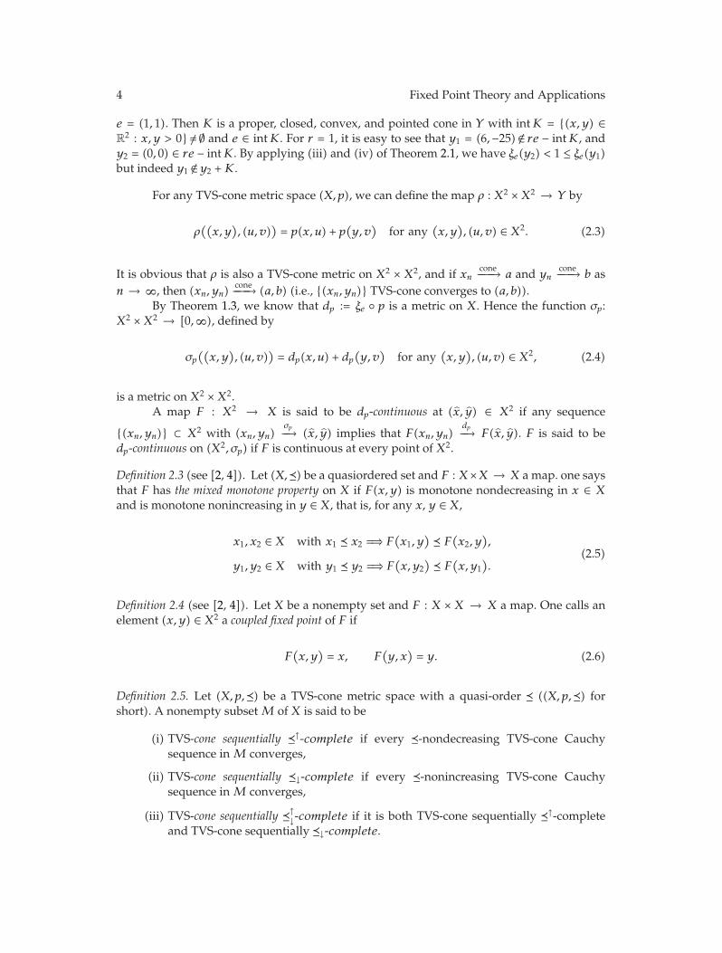
Remark 2.2. (a) Clearly, ξe(θ) = 0.(b) The reverse statement of (vi) in Theorem 2.1 (i.e., ξe(y2) ≤ ξe(y1) ⇒ y1 ∈ y2 + K)

does not hold in general. For example, let Y = R2, K = R2+ = {(x, y) ∈ R2 : x, y ≥ 0}, and


e = (1, 1). Then K is a proper, closed, convex, and pointed cone in Y with intK = {(x, y) ∈R2 : x, y > 0}/= ∅ and e ∈ intK. For r = 1, it is easy to see that y1 = (6,−25)/∈ re − intK, andy2 = (0, 0) ∈ re − intK. By applying (iii) and (iv) of Theorem 2.1, we have ξe(y2) < 1 ≤ ξe(y1)but indeed y1 /∈y2 +K.

For any TVS-cone metric space (X, p), we can define the map ρ : X2 ×X2 → Y by

ρ((x, y

), (u, v)

)= p(x, u) + p

(y, v

)for any

(x, y

), (u, v) ∈ X2. (2.3)

It is obvious that ρ is also a TVS-cone metric on X2 × X2, and if xncone−−−−→ a and yn

cone−−−−→ b asn → ∞, then (xn, yn)

cone−−−−→ (a, b) (i.e., {(xn, yn)} TVS-cone converges to (a, b)).By Theorem 1.3, we know that dp := ξe ◦ p is a metric on X. Hence the function σp:

X2 ×X2 → [0,∞), defined by

σp

((x, y

), (u, v)

)= dp(x, u) + dp

(y, v

)for any

(x, y

), (u, v) ∈ X2, (2.4)

is a metric on X2 ×X2.A map F : X2 → X is said to be dp-continuous at (x, y) ∈ X2 if any sequence

{(xn, yn)} ⊂ X2 with (xn, yn)σp−−→ (x, y) implies that F(xn, yn)

dp−−→ F(x, y). F is said to bedp-continuous on (X2, σp) if F is continuous at every point of X2.

Definition 2.3 (see [2, 4]). Let (X,�) be a quasiordered set and F : X×X → X a map. one saysthat F has the mixed monotone property on X if F(x, y) is monotone nondecreasing in x ∈ Xand is monotone nonincreasing in y ∈ X, that is, for any x, y ∈ X,

x1, x2 ∈ X with x1 � x2 =⇒ F(x1, y

)� F

(x2, y

),

y1, y2 ∈ X with y1 � y2 =⇒ F(x, y2

)� F

(x, y1

).

(2.5)

Definition 2.4 (see [2, 4]). Let X be a nonempty set and F : X × X → X a map. One calls anelement (x, y) ∈ X2 a coupled fixed point of F if

F(x, y

)= x, F

(y, x

)= y. (2.6)

Definition 2.5. Let (X, p,�) be a TVS-cone metric space with a quasi-order � ((X, p,�) forshort). A nonempty subset M of X is said to be

(i) TVS-cone sequentially �↑-complete if every �-nondecreasing TVS-cone Cauchysequence inM converges,

(ii) TVS-cone sequentially �↓-complete if every �-nonincreasing TVS-cone Cauchysequence inM converges,

(iii) TVS-cone sequentially �↑↓-complete if it is both TVS-cone sequentially �↑-complete

and TVS-cone sequentially �↓-complete.


Definition 2.6 (see [4, 18]). A function ϕ : [0,∞) → [0, 1) is said to be a MT-function if itsatisfies Mizoguchi-Takahashi’s condition (i.e., lim sups→ t+0 ϕ(s) < 1 for all t ∈ [0,∞)).

Clearly, if ϕ : [0,∞) → [0, 1) is a nondecreasing function, then ϕ is a MT-function.Notice that ϕ : [0,∞) → [0, 1) is a MT-function if and only if for each t ∈ [0,∞) there existrt ∈ [0, 1) and εt > 0 such that ϕ(s) ≤ rt for all s ∈ [t, t + εt); for more detail, see [4, Remark 2.5(iii)].

Very recently, Du and Wu [5] introduced and studied the concept of functions ofcontractive factor.

Definition 2.7 (see [5]). One says that ϕ : [0,∞) → [0, 1) is a function of contractive factor if forany strictly decreasing sequence {xn}n∈N

in [0,∞), one has

0 ≤ supn∈N

ϕ(xn) < 1. (2.7)

The following result tells us the relationship between MT-functions and functions ofcontractive factor.

Theorem 2.8. Any MT-function is a function of contractive factor.

Proof. Let ϕ : [0,∞) → [0, 1) be a MT-function, and let {xn}n∈Nbe a strictly decreasing

sequence in [0,∞). Then t0 := limn→∞ xn = infn∈N xn ≥ 0 exists. Since ϕ is a MT-function,there exist rt0 ∈ [0, 1) and εt0 > 0 such that ϕ(s) ≤ rt0 for all s ∈ [t0, t0 + εt0). On the other hand,there exists ∈ N, such that

t0 ≤ xn < t0 + εt0 (2.8)

for all n ∈ N with n ≥ . Hence ϕ(xn) ≤ rt0 for all n ≥ . Let

η := max{ϕ(x1), ϕ(x2), . . . , ϕ(x−1), rt0

}< 1. (2.9)

Then ϕ(xn) ≤ η for all n ∈ N, and hence 0 ≤ supn∈Nϕ(xn) ≤ η < 1. Therefore ϕ is a function of

contractive factor.

3. Coupled Fixed Point Theorems for Various Types ofNonlinear Contractive Maps

Definition 3.1. One says that κ : [0,∞) → (0, 1) is a function of strong contractive factor if forany strictly decreasing sequence {xn}n∈N

in [0,∞), one has

0 < supn∈N

κ(xn) < 1. (3.1)


It is quite obvious that if κ is a function of strong contractive factor, then κ is a functionof contractive factor but the reverse is not always true.

The following results are crucial to our proofs in this paper.

Lemma 3.2. A function of strong contractive factor can be structured by a function of contractivefactor.

Proof. Let ϕ : [0,∞) → [0, 1) be a function of contractive factor. Define κ(t) = (1 + ϕ(t))/2,t ∈ [0,∞). We claim that κ is a function of strong contractive factor. Clearly, 0 ≤ ϕ(t) < κ(t) < 1for all t ∈ [0,∞). Let {xn}n∈N

be a strictly decreasing sequence in [0,∞). Since ϕ is a functionof contractive factor, 0 ≤ supn∈N

ϕ(xn) < 1. Thus it follows that

0 < supn∈N

κ(xn) =12

[

1 + supn∈N

ϕ(xn)

]

< 1. (3.2)

Hence κ is a function of strong contractive factor.

Lemma 3.3. Let E be a t.v.s.,K a convex cone with intK/= ∅ in E, and a, b, c ∈ E. Then the followingstatements hold.

(i) If a�Kb and b�Kc, then a�Kc;

(ii) If a�Kb and b�Kc, then a�Kc;

(iii) If a�Kb and b�Kc, then a�Kc.

Proof. To see (i), since the set intK +K is open in E and K is a convex cone, we have

intK +K = int(intK +K) ⊆ intK. (3.3)

Since a�K b ⇐⇒ b − a ∈ K and b�K c ⇐⇒ c − b ∈ intK, it follows that

c − a = (c − b) + (b − a) ∈ intK +K ⊆ intK, (3.4)

which means that a�K c. The proofs of conclusions (ii) and(iii) are similar to (i).

Lemma 3.4 (see [4]). Let (X,�) be a quasiordered set and F : X2 → X a multivalued map havingthe mixed monotone property on X. Let x0, y0 ∈ X. Define two sequences {xn} and {yn} by

xn = F(xn−1, yn−1

),

yn = F(yn−1, xn−1

) (3.5)

for each n ∈ N. If x0 � x1 and y1 � y0, then {xn} is �-nondecreasing and {yn} is �-nonincreasing.


In this section, we first present the following new coupled fixed point theorem forfunctions of contractive factor in quasiordered cone metric spaces which is one of the mainresults of this paper.

Theorem 3.5. Let (X, p,�) be a TVS-cone sequentially �↑↓-complete metric space, F : X2 → X a

map having the mixed monotone property on X, and dp := ξe ◦ p. Assume that there exists a functionof contractive factor ϕ : [0,∞) → [0, 1) such that for any (x, y), (u, v) ∈ X2 with (u, v) � (x, y),

p(F(x, y

), F(u, v)

)�K

12ϕ(dp(x, u) + dp

(y, v

))ρ((x, y

), (u, v)

), (3.6)

and there exist x0, y0 ∈ X such that x0 � F(x0, y0) and F(y0, x0) � y0. Define the iterative sequence{(xn, yn)}n∈N∪{0} in X2 by xn = F(xn−1, yn−1) and yn = F(yn−1, xn−1) for n ∈ N. Then the followingstatements hold.

(a) There exists a nonempty subset D of X, such that (D, dp) is a complete metric space.

(b) There exists a nonempty subsetΩ ofX2, such that (Ω, σp) is a complete metric space, whereσp((x, y), (u, v)) := dp(x, u) + dp(y, v) for any (x, y), (u, v) ∈ X2. Moreover, if F is dp-continuous on (Ω, σp), then {(xn, yn)}n∈N∪{0} TVS-cone converges to a coupled fixed pointin Ω of F.

Proof. Since Y is a locally convex Hausdorff t.v.s. with its zero vector θ, let τ denote thetopology of Y and let Uτ be the base at θ consisting of all absolutely convex neighborhood ofθ. Let

L = { : is a Minkowski functional of U for U ∈ Uτ}. (3.7)

Then L is a family of seminorms on Y . For each ∈ L, let

V () ={y ∈ Y :

(y)< 1

}, (3.8)

and let

UL = {U : U = r1V (1) ∩ r2V (2) ∩ · · · ∩ rnV (n), rk > 0, k ∈ L, 1 ≤ k ≤ n, n ∈ N}. (3.9)

Then UL is a base at θ, and the topology ΓL generated by UL is the weakest topology for Ysuch that all seminorms in L are continuous and τ = ΓL. Moreover, given any neighborhoodOθ of θ, there exists U ∈ UL such that θ ∈ U ⊂ Oθ (see, e.g., [19, Theorem 12.4 in II.12, Page113]).

By Lemma 3.2, we can define a function of strong contractive factor κ : [0,∞) → [0, 1)by κ(t) = (ϕ(t) + 1)/2. Then 0 ≤ ϕ(t) < κ(t) < 1 for all t ∈ [0,∞). For any n ∈ N, letxn = F(xn−1, yn−1) and yn = F(yn−1, xn−1). Then, by Lemma 3.4, {xn} is �-nondecreasing and


{yn} is �-nonincreasing. So (xn, yn) � (xn+1, yn+1) and (yn+1, xn+1) � (yn, xn) for each n ∈ N.By (3.6), we obtain

p(x2, x1) = p(F(x1, y1

), F

(x0, y0

))

�K

12ϕ(dp(x1, x0) + dp

(y1, y0

))σ((x1, y1

),(x0, y0

))

=12ϕ(dp(x1, x0) + dp

(y1, y0

))[p(x1, x0) + p

(y1, y0

)],

(3.10)

p(y2, y1

)= p

(y1, y2

)

= p(F(y0, x0

), F

(y1, x1

))

�K

12ϕ(dp

(y0, y1

)+ dp(x0, x1)

)[p(y0, y1

)+ p(x0, x1)

]

=12ϕ(dp(x1, x0) + dp

(y1, y0

))[p(x1, x0) + p

(y1, y0

)].

(3.11)

By (3.10) and Theorem 2.1,

dp(x2, x1) = ξe(p(x2, x1)

)

≤ ξe

(12ϕ(dp(x1, x0) + dp

(y1, y0

))[p(x1, x0) + p

(y1, y0

)])

=12ϕ(dp(x1, x0) + dp

(y1, y0

))[dp(x1, x0) + dp

(y1, y0

)]

<12κ(dp(x1, x0) + dp

(y1, y0

))[dp(x1, x0) + dp

(y1, y0

)].

(3.12)

Similarly, by (3.11) and Theorem 2.1, we also have

dp

(y2, y1

)= ξe

(p(x2, x1)

)

≤ 12ϕ(dp(x1, x0) + dp

(y1, y0

))[dp(x1, x0) + dp

(y1, y0

)]

<12κ(dp(x1, x0) + dp

(y1, y0

))[dp(x1, x0) + dp

(y1, y0

)].

(3.13)

Combining (3.12) and (3.13), we get

dp(x2, x1) + dp

(y2, y1

)< κ

(dp(x1, x0) + dp

(y1, y0

))[dp(x1, x0) + dp

(y1, y0

)]. (3.14)


For each n ∈ N, let ξn = dp(xn, xn−1) + dp(yn, yn−1). Then ξ2 < κ(ξ1)ξ1. By induction, we canobtain the following. For each n ∈ N,

p(xn+1, xn)�K

12ϕ(ξn)

[p(xn, xn−1) + p

(yn, yn−1

)]; (3.15)

p(yn+1, yn

)�K

12ϕ(ξn)

[p(xn, xn−1) + p

(yn, yn−1

)]; (3.16)

dp(xn+1, xn) <12κ(ξn)ξn; (3.17)

dp

(yn+1, yn

)<

12κ(ξn)ξn; (3.18)

ξn+1 < κ(ξn)ξn. (3.19)

Since 0 < κ(t) < 1 for all t ∈ [0,∞), the sequence {ξn} is strictly decreasing in [0,∞)from (3.19). Since κ is a function of strong contractive factor, we have

0 < λ := supn∈N

κ(ξn) < 1. (3.20)

So ϕ(ξn) < κ(ξn) ≤ λ for all n ∈ N. We want to prove that {xn} is a �-nondecreasing TVS-coneCauchy sequence and {yn} is a �-nonincreasing TVS-cone Cauchy sequence in X. For eachn ∈ N, by (3.15), we have

p(xn+2, xn+1)�K

12λ[p(xn+1, xn) + p

(yn+1, yn

)]. (3.21)

Similarly, by (3.16), we obtain

p(yn+2, yn+1

)�K

12λ[p(xn+1, xn) + p

(yn+1, yn

)]. (3.22)

From (3.21) and (3.22), we get

p(xn+2, xn+1) + p(yn+2, yn+1

)�K λ

[p(xn+1, xn) + p

(yn+1, yn

)]for each n ∈ N. (3.23)


Hence it follows from (3.21), (3.22), and (3.23) that

p(xn+2, xn+1)�K

12λ[p(xn+1, xn) + p

(yn+1, yn

)]

�K

12λ2[p(xn, xn−1) + p

(yn, yn−1

)]

�K · · ·

�K

12λn

[p(x2, x1) + p

(y2, y1

)],

p(yn+2, yn+1

)�K

12λn

[p(x2, x1) + p

(y2, y1

)]for n ∈ N.

(3.24)

Therefore, for m,n ∈ N with m > n, we have

p(xm, xn)�K

m−1∑

j=n

p(xj+1, xj

)�K

λn−1

2(1 − λ)[p(x2, x1) + p

(y2, y1

)], (3.25)

p(ym, yn

)�K

m−1∑

j=n

p(yj+1, yj

)�K

λn−1

2(1 − λ)[p(x2, x1) + p

(y2, y1

)]. (3.26)

Given c ∈ Y with θ�K c (i.e., c ∈ intK = int(intK)), there exists a neighborhood Nθ of θsuch that c + Nθ ⊆ intK. Therefore, there exists Uc ∈ UL with Uc ⊆ Nθ such that c + Uc ⊆c +Nθ ⊆ intK, where

Uc = r1V (1) ∩ r2V (2) ∩ · · · ∩ rsV (s), (3.27)

for some ri > 0 and i ∈ L, 1 ≤ i ≤ s. Let

δc = min{ri : 1 ≤ i ≤ s} > 0,

η = max{i(p(x2, x1) + p

(y2, y1

)): 1 ≤ i ≤ s

}.

(3.28)

If η = 0, since each i is a seminorm, we have i(p(x2, x1) + p(y2, y1)) = 0 and

i

(

− λn−1

2(1 − λ)[p(x2, x1) + p

(y2, y1

)])

=λn−1

2(1 − λ)i(p(x2, x1) + p

(y2, y1

))= 0 < ri (3.29)


for all 1 ≤ i ≤ s and all n ∈ N. If η > 0, since λ ∈ (0, 1), limn→∞(λn−1/2(1 − λ)) = 0, and hencethere exists n0 ∈ N such that λn−1/2(1 − λ) < δc/η for all n ≥ n0. So, for each i ∈ {1, 2, . . . , s}and any n ≥ n0, we obtain

i

(

− λn−1

2(1 − λ)[p(x2, x1) + p

(y2, y1

)])

=λn−1

2(1 − λ)i(p(x2, x1) + p

(y2, y1

))

<δcηi(p(x2, x1) + p

(y2, y1

))

≤ δc

≤ ri.

(3.30)

Therefore for any n ≥ n0, −(λn−1/2(1 − λ))[p(x2, x1) + p(y2, y1)] ∈ riV (i) for all 1 ≤ i ≤ s, andhence −(λn−1/2(1 − λ))[p(x2, x1) + p(y2, y1)] ∈ Uc. So we obtain

c − λn−1

2(1 − λ)[p(x2, x1) + p

(y2, y1

)]∈ c +Uc ⊆ intK (3.31)

or

λn−1

2(1 − λ)[p(x2, x1) + p

(y2, y1

)]�K c (3.32)

for all n ≥ n0. For m,n ∈ N with m > n ≥ n0, by (3.25), (3.26), (3.32), and Lemma 3.3, weobtain

p(xm, xn)�K c,

p(ym, yn

)�K c.

(3.33)

Hence {xn} is a �-nondecreasing TVS-cone Cauchy sequence and {yn} is a �-nonincreasingTVS-cone Cauchy sequence in X. By the TVS-cone sequential �↑

↓-completeness of X, thereexist x, y ∈ X such that {xn} TVS-cone converges to x and {yn} TVS-cone converges to y.Therefore {(xn, yn)} TVS-cone converges to (x, y).

On the other hand, applying Theorem 1.4, we have the following:

{xn} is a � -nondecreasing Cauchy sequence in(X, dp

); (3.34)

{yn

}is a � -nonincreasing Cauchy sequence in

(X, dp

); (3.35)

dp(xn, x) −→ 0(or xn

dp−−→ x

)as n −→ ∞; (3.36)

dp

(yn, y

)−→ 0

(or yn

dp−−→ y

)as n −→ ∞. (3.37)


Since σp((xn, yn), (x, y) = dp(xn, x) + dp(yn, y) for all n ∈ N, by (3.36) and (3.37), we

have (xn, yn)σp−−→ (x, y) as n → ∞. Let D1 = {xn}n∈N∪{0} ∪ {x}, D2 = {yn}n∈N∪{0} ∪ {y}, and

Ω = D1 × D2. Then (D1, dp), (D2, dp), and (Ω, σp) are also complete metric spaces. Henceconclusion (a) holds.

Finally, in order to complete the proof of conclusion (b), we need to verify that (x, y) ∈Ω is a coupled fixed point of F. Let ε > 0 be given. Since F is dp-continuous on (Ω, σp) and(x, y) ∈ Ω, F is dp-continuous at (x, y). So there exists δ > 0 such that

dp

(F(x, y

), F(u, v)

)<

ε

2(3.38)

whenever (u, v) ∈ Ω with σp((x, y), (u, v)) < δ. Since xn

dp−−→ x and yn

dp−−→ y as n → ∞, forζ = min{ε/2, δ/2} > 0, there exists v0 ∈ N such that

dp(xn, x) < ζ, dp

(yn, y

)< ζ ∀n ∈ N with n ≥ v0. (3.39)

So, for each n ∈ N with n ≥ v0, by (3.39),

σp

((x, y

),(xn, yn

))= dp(xn, x) + dp

(yn, y

)< δ, (3.40)

and hence we have from (3.38) that

dp

(F(x, y

), F

(xn, yn

))<

ε

2. (3.41)

Therefore

dp

(F(x, y

), x

)≤ dp

(F(x, y

), xv0+1

)+ dp(xv0+1, x)

= dp

(F(x, y

), F

(xv0 , yv0

))+ dp(xv0+1, x)

<ε

2+ ζ

(by (3.39) and (3.41)

)

≤ ε.

(3.42)

Since ε is arbitrary, dp(F(x, y), x) = 0 or F(x, y) = x. Similarly, we can also prove that F(y, x) =y. So (x, y) ∈ Ω is a coupled fixed point of F. The proof is finished.

The following conclusions are immediate from Theorems 2.8 and 3.5.

Theorem 3.6. Let (X, p,�) be a TVS-cone sequentially �↑↓-complete metric space, F : X2 → X a map

having the mixed monotone property on X, and dp := ξe ◦ p. Assume that there exists aMT-functionϕ : [0,∞) → [0, 1) such that for any (x, y), (u, v) ∈ X2 with (u, v) � (x, y),

p(F(x, y

), F(u, v)

)�K

12ϕ(dp(x, u) + dp

(y, v

))ρ((x, y

), (u, v)

), (3.43)




(b) There exists a nonempty subset Ω of X2, such that (Ω, σp) is a complete metric space.Moreover, if F is dp-continuous on (Ω, σp), then {(xn, yn)}n∈N∪{0} TVS-cone converges toa coupled fixed point in Ω of F.

Theorem 3.7. Let (X, p,�) be a TVS-cone sequentially �↑↓-complete metric space, F : X2 → X a map

having the mixed monotone property on X, and dp := ξe ◦ p. Assume that there exists a nonnegativenumber γ < 1 such that for any (x, y), (u, v) ∈ X2 with (u, v) � (x, y),

p(F(x, y

), F(u, v)

)�K

γ

2ρ((x, y

), (u, v)

), (3.44)



(b) There exists a nonempty subset Ω of X2, such that (Ω, σp) is a complete metric space.Moreover, if F is dp-continuous on (Ω, σp), then {(xn, yn)}n∈N∪{0} TVS-cone converges toa coupled fixed point in Ω of F.

Remark 3.8. (a) Theorems 3.5 and 3.6 all generalize and improve [4, Theorem 2.8] and someresults in [2, 9, 11].

(b) Theorems 3.5–3.7 all generalize Bhaskar-Lakshmikantham’s coupled fixed pointstheorem (i.e., Theorem BL).

Finally, we focus our research on TVS-cone metric spaces.

Theorem 3.9. Let (X, p) be a TVS-cone complete metric space, F : X2 → X a map, and dp := ξe ◦p.Assume that there exists a function of contractive factor ϕ : [0,∞) → [0, 1) such that for any(x, y), (u, v) ∈ X2

p(F(x, y

), F(u, v)

)�K

12ϕ(dp(x, u) + dp

(y, v

))ρ((x, y

), (u, v)

). (3.45)

Let x0, y0 ∈ X. Define the iterative sequence {(xn, yn)}n∈N∪{0} in X2 by xn = F(xn−1, yn−1) andyn = F(yn−1, xn−1) for n ∈ N. Then the following statements hold.


(b) There exists a nonempty subset Ω of X2, such that (Ω, σp) is a complete metric space.

(c) F has a unique coupled fixed point in Ω. Moreover, {(xn, yn)}n∈N∪{0} TVS-cone convergesto the coupled fixed point of F.


Proof. For any (x, y), (u, v) ∈ X2, by (3.45) and Theorem 2.1, we obtain

dp

(F(x, y

), F(u, v)

)≤ 1

2ϕ(dp(x, u) + dp

(y, v

))[dp(x, u) + dp

(y, v

)]

=12ϕ(σp

((x, y

), (u, v)

))σp

((x, y

), (u, v)

)

<12σp

((x, y

), (u, v)

).

(3.46)

From (3.46), we know that F is dp-continuous on (X2, σp). Following the same argument asin the proof of Theorem 3.5, we can prove that conclusions (a) and (b) hold and there exists(x, y) ∈ Ω, such that {(xn, yn)}n∈N∪{0} TVS-cone converges to (x, y) and (x, y) is a coupledfixed point of F. To complete the proof, it suffices to show the uniqueness of the coupled fixedpoint of F. On the contrary, suppose that there exists (u, v) ∈ X ×X, such that u = F(u, v) andv = F(v, u). By (3.46), we have

dp(x, u) = dp

(F(x, y

), F(u, v)

)<

12[dp(x, u) + dp

(y, v

)],

dp

(y, v

)= dp

(F(y, x

), F(v, u)

)<

12[dp(x, u) + dp

(y, v

)].

(3.47)

So, it follows from (3.47) that

dp(x, u) + dp

(y, v

)< dp(x, u) + dp

(y, v

), (3.48)

which leads to a contradiction. The proof is completed.

The following results are immediate from Theorem 3.9.

Theorem 3.10. Let (X, p) be a TVS-cone complete metric space, F : X2 → X a map, and dp := ξe◦p.Assume that there exists a MT-function ϕ : [0,∞) → [0, 1) such that for any (x, y), (u, v) ∈ X2,

p(F(x, y

), F(u, v)

)�K

12ϕ(dp(x, u) + dp

(y, v

))ρ((x, y

), (u, v)

). (3.49)






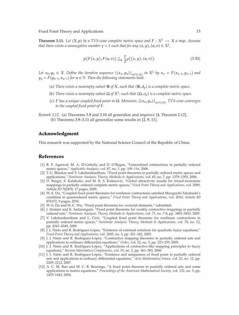
Theorem 3.11. Let (X, p) be a TVS-cone complete metric space and F : X2 → X a map. Assumethat there exists a nonnegative number γ < 1 such that for any (x, y), (u, v) ∈ X2,

p(F(x, y

), F(u, v)

)�K

γ

2ρ((x, y

), (u, v)

). (3.50)





Remark 3.12. (a) Theorems 3.9 and 3.10 all generalize and improve [4, Theorem 2.12].(b) Theorems 3.9–3.11 all generalize some results in [2, 9, 11].

Acknowledgment

This research was supported by the National Science Council of the Republic of China.

References

[1] R. P. Agarwal, M. A. El-Gebeily, and D. O’Regan, “Generalized contractions in partially orderedmetric spaces,” Applicable Analysis, vol. 87, no. 1, pp. 109–116, 2008.

[2] T. G. Bhaskar and V. Lakshmikantham, “Fixed point theorems in partially ordered metric spaces andapplications,” Nonlinear Analysis: Theory, Methods & Applications, vol. 65, no. 7, pp. 1379–1393, 2006.

[3] D. Burgic, S. Kalabusic, and M. R. S. Kulenovic, “Global attractivity results for mixed-monotonemappings in partially ordered complete metric spaces,” Fixed Point Theory and Applications, vol. 2009,Article ID 762478, 17 pages, 2009.

[4] W.-S. Du, “Coupled fixed point theorems for nonlinear contractions satisfied Mizoguchi-Takahashi’scondition in quasiordered metric spaces,” Fixed Point Theory and Applications, vol. 2010, Article ID876372, 9 pages, 2010.

[5] W.-S. Du and H.-C. Wu, “Fixed point theorems for vectorial elements,” submitted.[6] J. Harjani and K. Sadarangani, “Fixed point theorems for weakly contractive mappings in partially

ordered sets,” Nonlinear Analysis: Theory, Methods & Applications, vol. 71, no. 7-8, pp. 3403–3410, 2009.[7] V. Lakshmikantham and L. Ciric, “Coupled fixed point theorems for nonlinear contractions in

partially ordered metric spaces,” Nonlinear Analysis: Theory, Methods & Applications, vol. 70, no. 12,pp. 4341–4349, 2009.

[8] J. J. Nieto and R. Rodrıguez-Lopez, “Existence of extremal solutions for quadratic fuzzy equations,”Fixed Point Theory and Applications, vol. 2005, no. 3, pp. 321–342, 2005.

[9] J. J. Nieto and R. Rodrıguez-Lopez, “Contractive mapping theorems in partially ordered sets andapplications to ordinary differential equations,” Order, vol. 22, no. 3, pp. 223–239, 2005.

[10] J. J. Nieto and R. Rodrıguez-Lopez, “Applications of contractive-like mapping principles to fuzzyequations,” Revista Matematica Complutense, vol. 19, no. 2, pp. 361–383, 2006.

[11] J. J. Nieto and R. Rodrıguez-Lopez, “Existence and uniqueness of fixed point in partially orderedsets and applications to ordinary differential equations,” Acta Mathematica Sinica, vol. 23, no. 12, pp.2205–2212, 2007.

[12] A. C. M. Ran and M. C. B. Reurings, “A fixed point theorem in partially ordered sets and someapplications to matrix equations,” Proceedings of the American Mathematical Society, vol. 132, no. 5, pp.1435–1443, 2004.


[13] Y. Wu, “New fixed point theorems and applications of mixed monotone operator,” Journal ofMathematical Analysis and Applications, vol. 341, no. 2, pp. 883–893, 2008.

[14] W.-S. Du, “A note on cone metric fixed point theory and its equivalence,” Nonlinear Analysis: Theory,Methods & Applications, vol. 72, no. 5, pp. 2259–2261, 2010.

[15] L.-G. Huang and X. Zhang, “Cone metric spaces and fixed point theorems of contractive mappings,”Journal of Mathematical Analysis and Applications, vol. 332, no. 2, pp. 1468–1476, 2007.

[16] G. Chen, X. Huang, and X. Yang, Vector Optimization, vol. 541 of Lecture Notes in Economics andMathematical Systems, Springer, Berlin, Germany, 2005.

[17] W.-S. Du, “On some nonlinear problems induced by an abstract maximal element principle,” Journalof Mathematical Analysis and Applications, vol. 347, no. 2, pp. 391–399, 2008.

[18] W.-S. Du, “Some new results and generalizations in metric fixed point theory,” Nonlinear Analysis:Theory, Methods & Applications, vol. 73, pp. 1439–1446, 2010.

[19] A. E. Taylor and D. C. Lay, Introduction to Functional Analysis, JohnWiley & Sons, New York, NY, USA,2nd edition, 1980.

nonlinear contractive conditions for coupled cone fixed point … · of nonlinear contractive maps...

Documents