Non-parametric calibration of jump-diffusionmodels.

Rama Cont & Peter TANKOV

Centre de Mathematiques Appliquees

CNRS – Ecole Polytechnique

Rama.Cont@polytechnique.org Peter.Tankov@polytechnique.org

http://www.cmap.polytechnique.fr/˜rama/

1

References:

R Cont , P Tankov (2002) Calibration of jump-diffusion option

pricing models: a robust non-parametric approach, Rapport

Interne CMAP No. 490

Download from:

http://www.cmap.polytechnique.fr/˜rama/

2

Outline:

• Overview of exponential Levy models.

• The calibration problem for exp Levy models.

• Ill posedness and instability of least squares calibration.

• Regularization using convex penalization.

• Relative entropy for Levy processes.

• Numerical implementation.

• Tests on simulated data.

• Empirical results for DAX options.

• Conclusion and perspectives.

3

Jump diffusion models for option pricing

Time homogeneous jumps with finite intensity:

St = S0 exp(rt+ γt+ σWt +

Nt∑

i=1

Yi)

σ : Volatility coefficient

Nt : Number of jumps : Poisson process with intensity λ

Yi : Jump sizes : IID random variables with density f(.)

Parameters: σ > 0, frequency of jumps λ, probability density of

jump sizes f(.)

Definition: ν = λf is called the Levy density.

Extensions: infinite jump rates, time inhomogeneity.

4

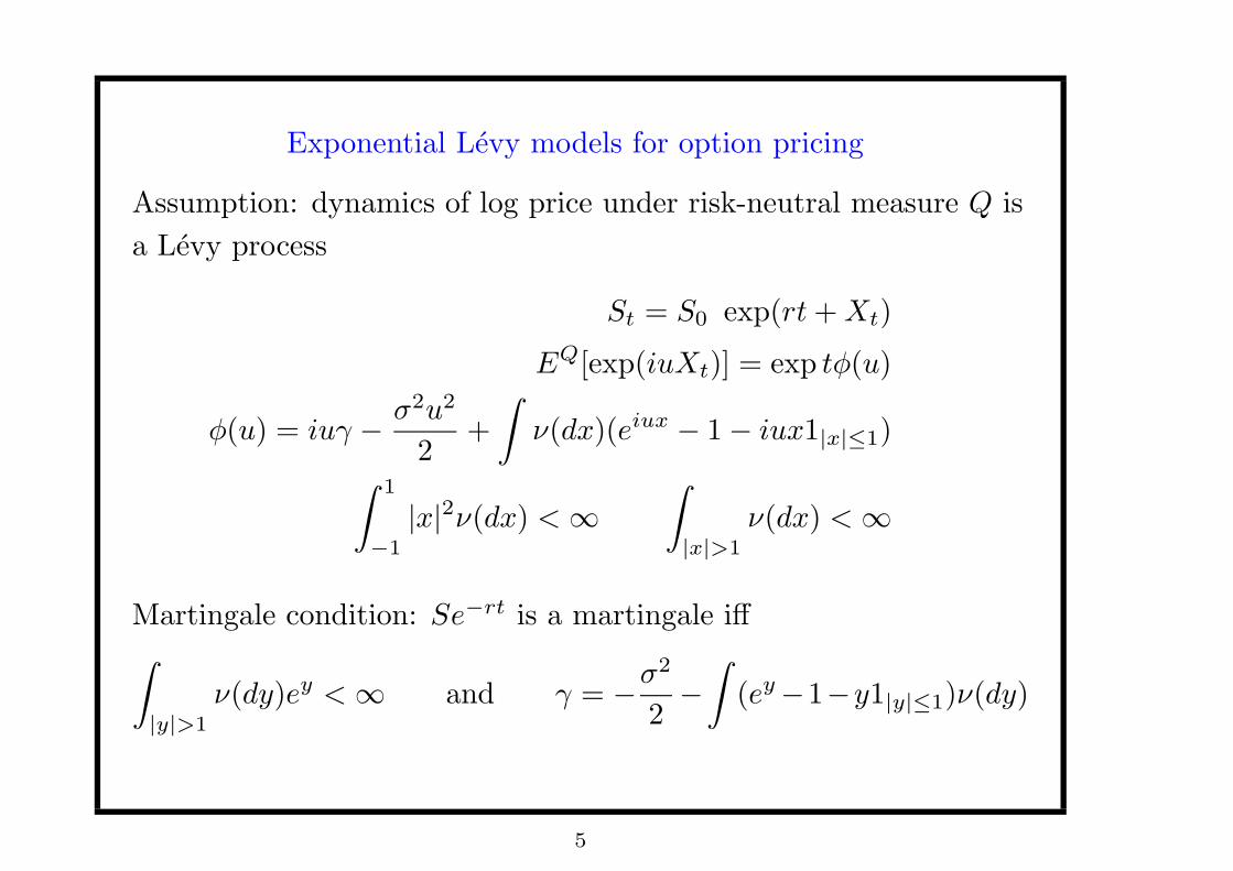
Exponential Levy models for option pricing

Assumption: dynamics of log price under risk-neutral measure Q is

a Levy process

St = S0 exp(rt+Xt)

EQ[exp(iuXt)] = exp tφ(u)

φ(u) = iuγ −σ2u2

2+

∫

ν(dx)(eiux − 1− iux1|x|≤1)

∫ 1

−1

|x|2ν(dx) <∞

∫

|x|>1

ν(dx) <∞

Martingale condition: Se−rt is a martingale iff∫

|y|>1

ν(dy)ey <∞ and γ = −σ2

2−

∫

(ey−1−y1|y|≤1)ν(dy)

5

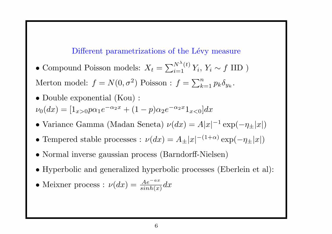
Different parametrizations of the Levy measure

• Compound Poisson models: Xt =∑Nλ(t)

i=1 Yi, Yi ∼ f IID )

Merton model: f = N(0, σ2) Poisson : f =∑n

k=1 pkδyk .

• Double exponential (Kou) :

ν0(dx) = [1x>0pα1e−α2x + (1− p)α2e

−α2x1x<0]dx

• Variance Gamma (Madan Seneta) ν(dx) = A|x|−1 exp(−η±|x|)

• Tempered stable processes : ν(dx) = A±|x|−(1+α) exp(−η±|x|)

• Normal inverse gaussian process (Barndorff-Nielsen)

• Hyperbolic and generalized hyperbolic processes (Eberlein et al):

• Meixner process : ν(dx) = Ae−ax

sinh(x)dx

6

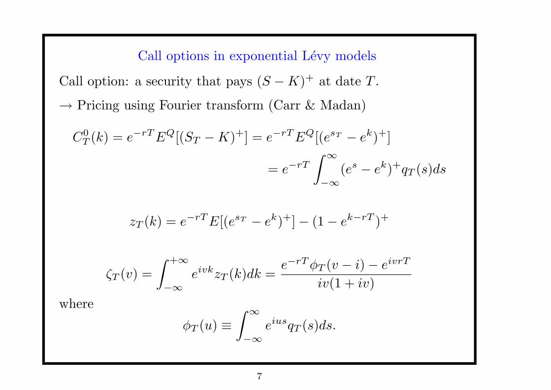
Call options in exponential Levy models

Call option: a security that pays (S −K)+ at date T .

→ Pricing using Fourier transform (Carr & Madan)

C0T (k) = e−rTEQ[(ST −K)+] = e−rTEQ[(esT − ek)+]

= e−rT∫ ∞

−∞

(es − ek)+qT (s)ds

zT (k) = e−rTE[(esT − ek)+]− (1− ek−rT )+

ζT (v) =

∫ +∞

−∞

eivkzT (k)dk =e−rTφT (v − i)− eivrT

iv(1 + iv)

where

φT (u) ≡

∫ ∞

−∞

eiusqT (s)ds.

7

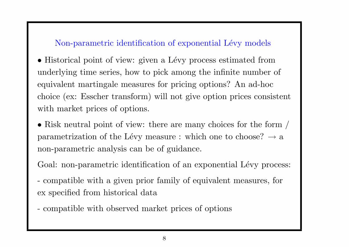
Non-parametric identification of exponential Levy models

• Historical point of view: given a Levy process estimated from

underlying time series, how to pick among the infinite number of

equivalent martingale measures for pricing options? An ad-hoc

choice (ex: Esscher transform) will not give option prices consistent

with market prices of options.

• Risk neutral point of view: there are many choices for the form /

parametrization of the Levy measure : which one to choose? → a

non-parametric analysis can be of guidance.

Goal: non-parametric identification of an exponential Levy process:

- compatible with a given prior family of equivalent measures, for

ex specified from historical data

- compatible with observed market prices of options

8

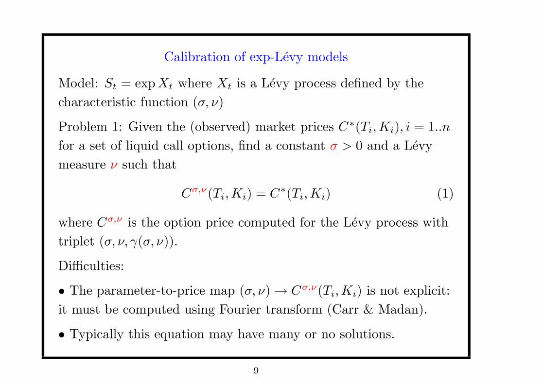
Calibration of exp-Levy models

Model: St = expXt where Xt is a Levy process defined by the

characteristic function (σ, ν)

Problem 1: Given the (observed) market prices C∗(Ti,Ki), i = 1..n

for a set of liquid call options, find a constant σ > 0 and a Levy

measure ν such that

Cσ,ν(Ti,Ki) = C∗(Ti,Ki) (1)

where Cσ,ν is the option price computed for the Levy process with

triplet (σ, ν, γ(σ, ν)).

Difficulties:

• The parameter-to-price map (σ, ν)→ Cσ,ν(Ti,Ki) is not explicit:

it must be computed using Fourier transform (Carr & Madan).

• Typically this equation may have many or no solutions.

9

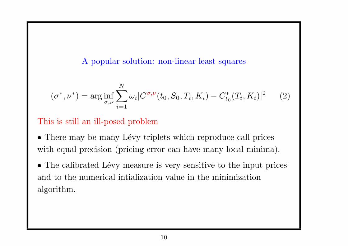
A popular solution: non-linear least squares

(σ∗, ν∗) = arg infσ,ν

N∑

i=1

ωi|Cσ,ν(t0, S0, Ti,Ki)− C∗t0(Ti,Ki)|

2 (2)

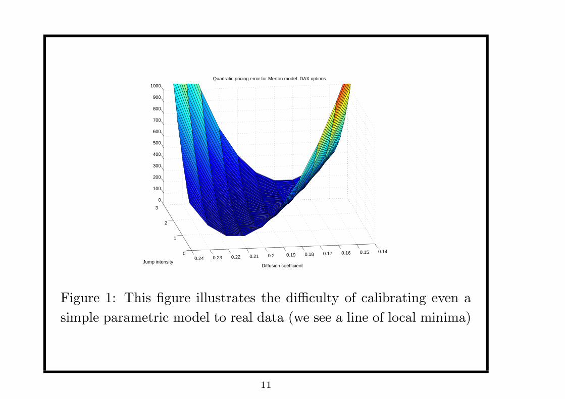
This is still an ill-posed problem

• There may be many Levy triplets which reproduce call prices

with equal precision (pricing error can have many local minima).

• The calibrated Levy measure is very sensitive to the input prices

and to the numerical intialization value in the minimization

algorithm.

10

0

1

2

3

0.140.150.160.170.180.190.20.210.220.230.24

0

100

200

300

400

500

600

700

800

900

1000

Quadratic pricing error for Merton model: DAX options.

Diffusion coefficientJump intensity

Figure 1: This figure illustrates the difficulty of calibrating even a

simple parametric model to real data (we see a line of local minima)

11

−0.8 −0.6 −0.4 −0.2 0 0.2 0.4 0.60

2

4

6

8

10

12

14

16

18

20 Calibrated Lévy density: no regularization

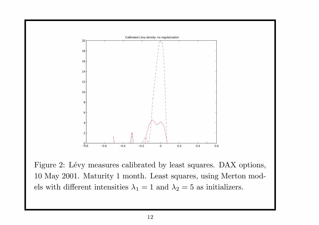
Figure 2: Levy measures calibrated by least squares. DAX options,

10 May 2001. Maturity 1 month. Least squares, using Merton mod-

els with different intensities λ1 = 1 and λ2 = 5 as initializers.

12

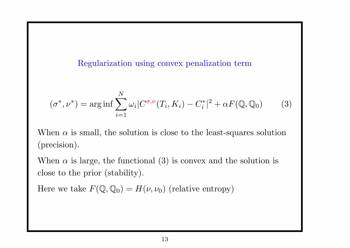
Regularization using convex penalization term

(σ∗, ν∗) = arg infN∑

i=1

ωi|Cσ,ν(Ti,Ki)− C∗i |

2 + αF (Q,Q0) (3)

When α is small, the solution is close to the least-squares solution

(precision).

When α is large, the functional (3) is convex and the solution is

close to the prior (stability).

Here we take F (Q,Q0) = H(ν, ν0) (relative entropy)

13

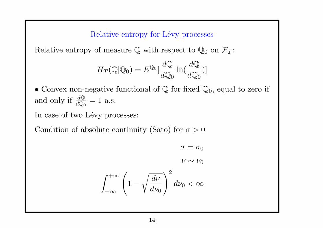
Relative entropy for Levy processes

Relative entropy of measure Q with respect to Q0 on FT :

HT (Q|Q0) = EQ0 [dQ

dQ0ln(

dQ

dQ0)]

• Convex non-negative functional of Q for fixed Q0, equal to zero if

and only if dQdQ0

= 1 a.s.

In case of two Levy processes:

Condition of absolute continuity (Sato) for σ > 0

σ = σ0

ν ∼ ν0

∫ +∞

−∞

(

1−

√

dν

dν0

)2

dν0 <∞

14

HT (Q|Q0) =T

2σ2

{

γ − γ0 −

∫ 1

−1

x(ν − ν0)(dx)

}2

+

T

∫ ∞

−∞

(dν

dν0log(

dν

dν0) + 1−

dν

dν0)ν0(dx)

Here the first term penalizes the difference of drifts and the second

one penalizes the difference of Levy measures.

If Q and Q0 are martingale measures, the first term becomes

T

2σ2

{∫ ∞

−∞

(ex − 1)(ν − ν0)(dx)

}2

and the relative entropy only depends on ν and ν0, i.e.

H(Q|Q0) = H(ν, ν0)

15

Properties of relative entropy

• Preserves absolute continuity

• H(ν, ν0) is a convex non-negative functional of ν for fixed ν0,

equal to zero iff ν = ν0 almost everywhere

• Easy to compute

• Corresponds to adding the least possible amount of information

to the prior

• Widely used in the literature

16

Relation to other entropy-based calibration algorithms

• Weighted Monte Carlo (WMC) method by Avellaneda & al.

Q = arg minQ∼Q0

E(Q,Q0) +

n∑

i=1

|C∗(Ti,Ki)− EQ(S(Ti)−Ki)+|2

where Q and Q0 are probability measures on a finite set of

trajectories, simulated from the Q0 by Monte Carlo.

Principal differences:

• In the WMC method the optimization is done over the measure

Q. Here it is done over the parameters σ, ν of the infinitesimal

generator.

• The result of WMC is a set of weights Q(ω) over a (finite) set

of paths. In our case the result is a process, defined by its local

characteristics γ(σ, ν), σ, ν.

• Consequence of 1): In our approach the calibrated measure

17

belongs to the class of risk-neutral measures, corresponding to

Levy processes/ jump diffusions.

• In WMC discretization is essential to make the problem

meaningful: the continuous problem does not make sense. Here

the limit is well defined and discretization is only used in the

numerical implementation. In particular the continuum limit is

not singular.

• Under this approach other options can only be priced by Monte

Carlo using the same sample paths, while our method allows

using PIDE methods or Monte Carlo methods for pricing. In

particular Monte Carlo pricing can be done with an arbitrary

number of paths.

18

Regularization using relative entropy

ν∗ = arg inf αH(ν, ν0) +

N∑

i=1

ωi(Cν(Ti,Ki)− C∗(Ti,Ki))

2 (4)

Properties of solution:

• Depends continuously on the input prices

• Does not depend on the initial measure (when α is large

enough)

• The entropic regularization makes the calibrated measure more

smooth

19

−0.8 −0.6 −0.4 −0.2 0 0.2 0.4 0.60

0.5

1

1.5

2

2.5

3

3.5

4

4.5

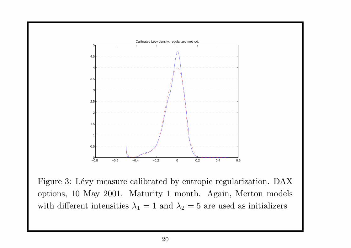
5Calibrated Lévy density: regularized method.

Figure 3: Levy measure calibrated by entropic regularization. DAX

options, 10 May 2001. Maturity 1 month. Again, Merton models

with different intensities λ1 = 1 and λ2 = 5 are used as initializers

20

Numerical implementation: choice of the prior measure Q0

• Based on historical estimation (in this case we obtain the

risk-neutral measure, closest to the historical one)

• Based on the calibrated measure of the day before. This

ensures smooth variation with calendar time.

• From the same dataset, using pre-calibration. In this case we

first calibrate a simple parametric model (i.e. Merton’s model)

using least squares and then use it as prior. Here, the prior

does not contain any additional information and is only used to

regularize the problem.

21

Numerical implementation: choice of the regularization parameter

ν∗ = arg inf αH(ν, ν0) +N∑

i=1

ωi(Cν(Ti,Ki)− C∗(Ti,Ki))

2 (5)

Small α: high precision in calibration, low stability (non convex).

High α: low precision, high stability.

Typically the a posteriori error level ε(α) increases with α.

Idea: choose α such that the a posteriori error (calibration error)

has the same level as the a priori error (error on input prices).

Morozov discrepancy principle : given the ”noise” level ε0 on the

input prices, choose α > 0 such that ε(α) ' ε0.

Typically ε0 is due to bid/ask spreads.

22

Numerical implementation: other issues

• The weights ωi of different prices must reflect relative liquidity

of these options: a simple solution is to take ωi =1

V ega2

i

• The Levy measure is discretized on a uniform grid in order to

use FFT.

• An explicit representation of the gradient of the minimization

functional allows to use a gradient based optimization method

to solve the minimization problem.

23

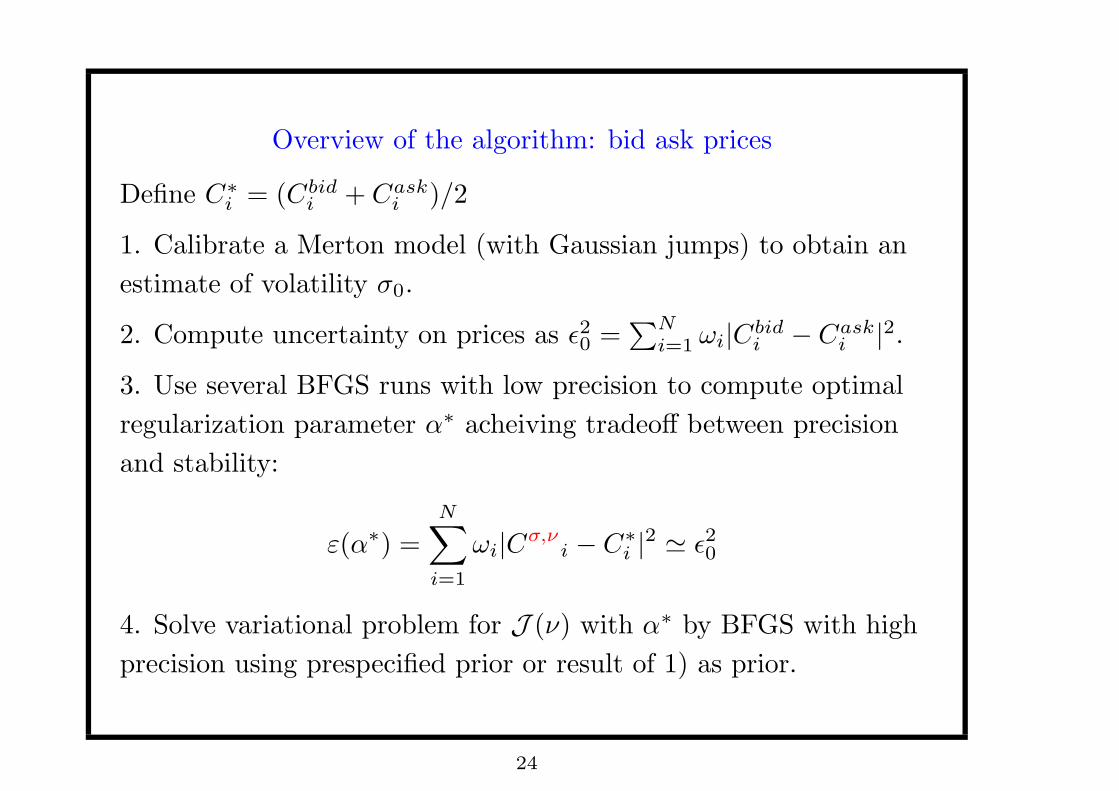
Overview of the algorithm: bid ask prices

Define C∗i = (Cbidi + Cask

i )/2

1. Calibrate a Merton model (with Gaussian jumps) to obtain an

estimate of volatility σ0.

2. Compute uncertainty on prices as ε20 =∑N

i=1 ωi|Cbidi − Cask

i |2.

3. Use several BFGS runs with low precision to compute optimal

regularization parameter α∗ acheiving tradeoff between precision

and stability:

ε(α∗) =

N∑

i=1

ωi|Cσ,ν

i − C∗i |2 ' ε20

4. Solve variational problem for J (ν) with α∗ by BFGS with high

precision using prespecified prior or result of 1) as prior.

24

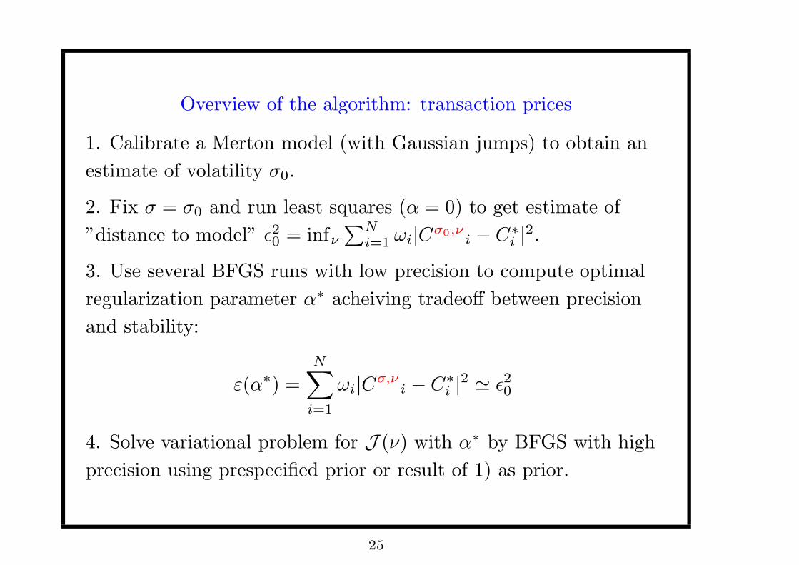
Overview of the algorithm: transaction prices

1. Calibrate a Merton model (with Gaussian jumps) to obtain an

estimate of volatility σ0.

2. Fix σ = σ0 and run least squares (α = 0) to get estimate of

”distance to model” ε20 = infν∑N

i=1 ωi|Cσ0,ν

i − C∗i |2.

3. Use several BFGS runs with low precision to compute optimal

regularization parameter α∗ acheiving tradeoff between precision

and stability:

ε(α∗) =

N∑

i=1

ωi|Cσ,ν

i − C∗i |2 ' ε20

4. Solve variational problem for J (ν) with α∗ by BFGS with high

precision using prespecified prior or result of 1) as prior.

25

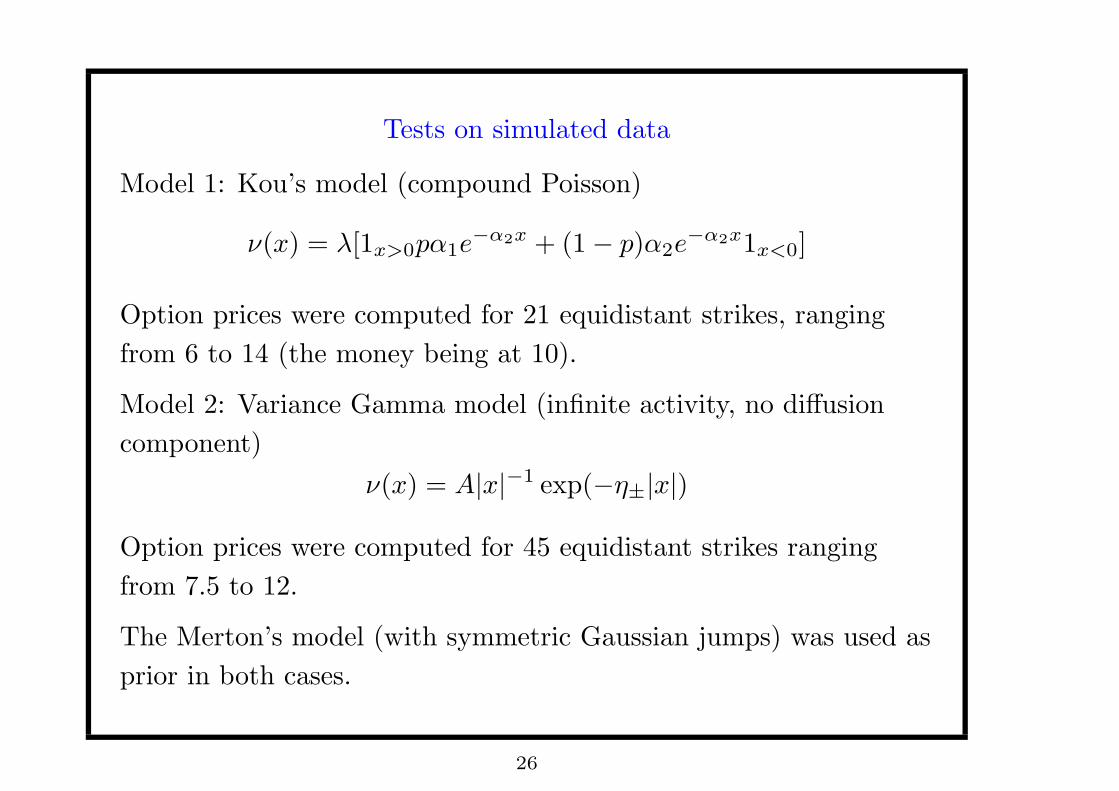
Tests on simulated data

Model 1: Kou’s model (compound Poisson)

ν(x) = λ[1x>0pα1e−α2x + (1− p)α2e

−α2x1x<0]

Option prices were computed for 21 equidistant strikes, ranging

from 6 to 14 (the money being at 10).

Model 2: Variance Gamma model (infinite activity, no diffusion

component)

ν(x) = A|x|−1 exp(−η±|x|)

Option prices were computed for 45 equidistant strikes ranging

from 7.5 to 12.

The Merton’s model (with symmetric Gaussian jumps) was used as

prior in both cases.

26

6 7 8 9 10 11 12 13 140.1

0.15

0.2

0.25

0.3

0.35

0.4

0.45

0.5

Strike

Impl

ied

vola

tility

simulatedcalibrated

0.75 0.8 0.85 0.9 0.95 1 1.05 1.1 1.15 1.20.05

0.1

0.15

0.2

0.25

0.3

0.35

0.4

0.45

Strike

Impl

ied

vola

tility

Variance gammaCalibrated

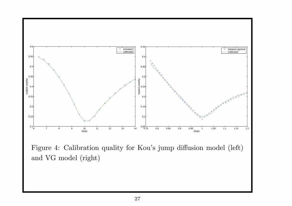
Figure 4: Calibration quality for Kou’s jump diffusion model (left)

and VG model (right)

27

−0.5 −0.4 −0.3 −0.2 −0.1 0 0.1 0.2 0.3 0.4 0.50

0.5

1

1.5

2

2.5

3

3.5

4

4.5

5priortruecalibrated

−0.5 −0.4 −0.3 −0.2 −0.1 0 0.1 0.2 0.3 0.4 0.50

0.5

1

1.5

2

2.5

3

3.5

4

4.5

5priortruecalibrated

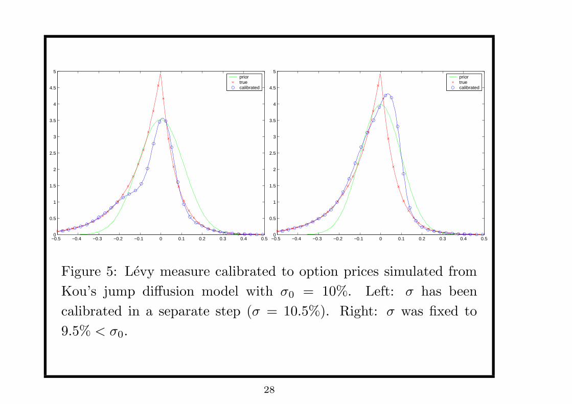
Figure 5: Levy measure calibrated to option prices simulated from

Kou’s jump diffusion model with σ0 = 10%. Left: σ has been

calibrated in a separate step (σ = 10.5%). Right: σ was fixed to

9.5% < σ0.

28

−0.5 −0.4 −0.3 −0.2 −0.1 0 0.1 0.2 0.3 0.4 0.50

1

2

3

4

5

6

7

8

9

10Calibrated compound Poisson Levy measureTrue variance gamma Levy measure

−0.5 −0.4 −0.3 −0.2 −0.1 0 0.1 0.2 0.3 0.4 0.50

5

10

15

20

25

30

35

40Calibrated compound Poisson Levy measureTrue variance gamma Levy measure

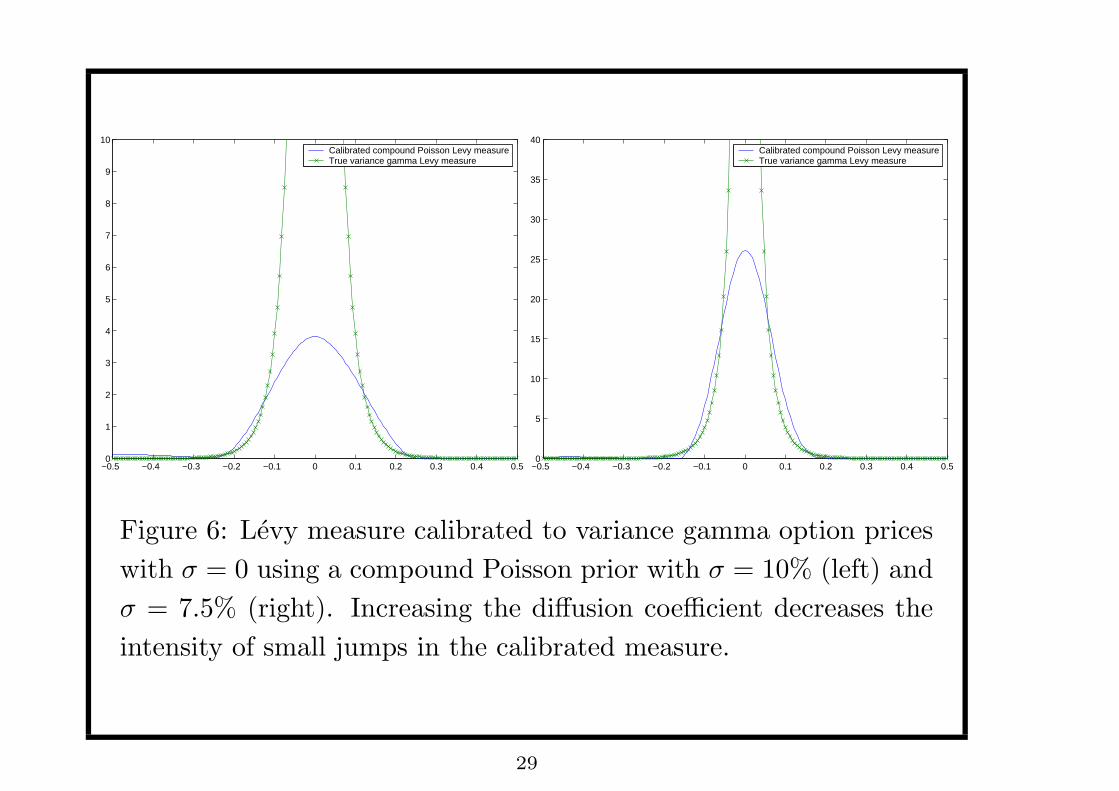
Figure 6: Levy measure calibrated to variance gamma option prices

with σ = 0 using a compound Poisson prior with σ = 10% (left) and

σ = 7.5% (right). Increasing the diffusion coefficient decreases the

intensity of small jumps in the calibrated measure.

29

Summary of empirical results

The calibrated Levy measures we obtain are strongly asymmetric:

the distribution of jump sizes is highly skewed towards negative

values.

A small intensity of jumps λ can be sufficient for explaining the

shape of the implied volatility for small maturities: empirically

λ ' 1

Regularization by entropy strongly reduces sensitivity of results to

the initialization: stable numerical results.

30

−0.8 −0.6 −0.4 −0.2 0 0.2 0.4 0.60

0.5

1

1.5

2

2.5

3

3.5

4

4.5

5Calibrated Lévy density: regularized method.

−0.8 −0.6 −0.4 −0.2 0 0.2 0.4 0.610

−7

10−6

10−5

10−4

10−3

10−2

10−1

100

101

Calibrated Lévy density: regularized method.

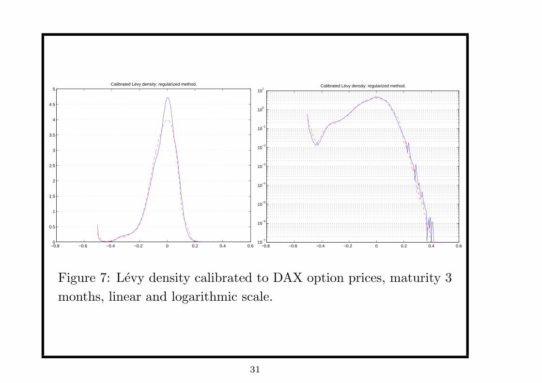
Figure 7: Levy density calibrated to DAX option prices, maturity 3

months, linear and logarithmic scale.

31

3500 4000 4500 5000 5500 6000 6500 7000 75000

0.2

0.4

0.6

0.8

1

1.2

Strike

Impl

ied

vola

tility

Calibration quality for different maturities. DAX options, 11 May 2001

Maturity 8 days, marketMaturity 8 days, modelMaturity 36 days, marketMaturity 36 days, modelMaturity 71 days, marketMaturity 71 days, model

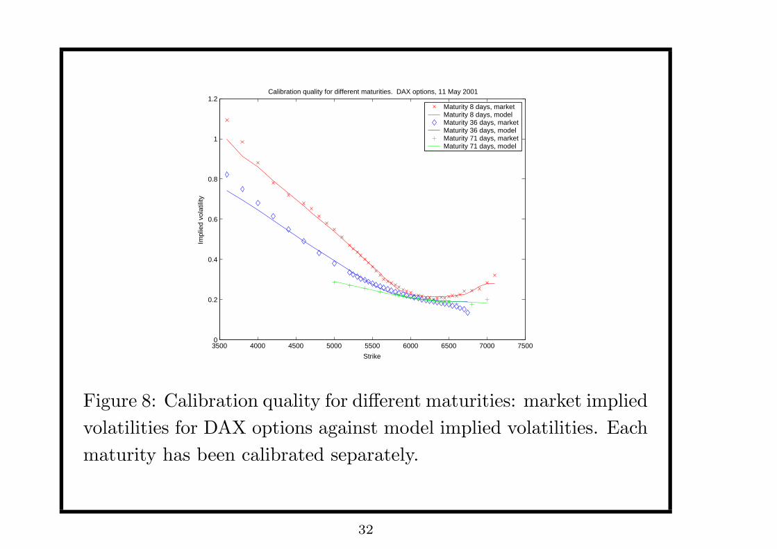
Figure 8: Calibration quality for different maturities: market implied

volatilities for DAX options against model implied volatilities. Each

maturity has been calibrated separately.

32

−1 −0.5 0 0.50

0.5

1

1.5

2

2.5

3

3.5

4Calibrated Levy measures for different maturities. DAX options, 11 May 2001

Maturity 8 daysMaturity 36 daysMaturity 71 daysPrior

−1 −0.5 0 0.510

−6

10−5

10−4

10−3

10−2

10−1

100

101

Calibrated Levy measures for different maturities, log scale. DAX options, 11 May 2001

Maturity 8 daysMaturity 36 daysMaturity 71 daysPrior

Figure 9: Levy measures calibrated to DAX option prices for three

different maturieis, linear and logarithmic scale.

33

−0.6 −0.1 0.40

0.5

1

1.5

2

2.5

3

3.5

4

4.5

5Levy measure calibrated for shortest maturity. DAX options, different dates

11 May 2001, 8 days11 June 2001, 4 days 11 July 2001, 9 daysPrior

−1 −0.8 −0.6 −0.4 −0.2 0 0.2 0.40

0.5

1

1.5

2

2.5

3

3.5

4Levy measure calibrated for second shortest maturity. DAX options, different dates

11 May 2001, 36 days11 June 2001, 39 days11 July 2001, 37 daysPrior

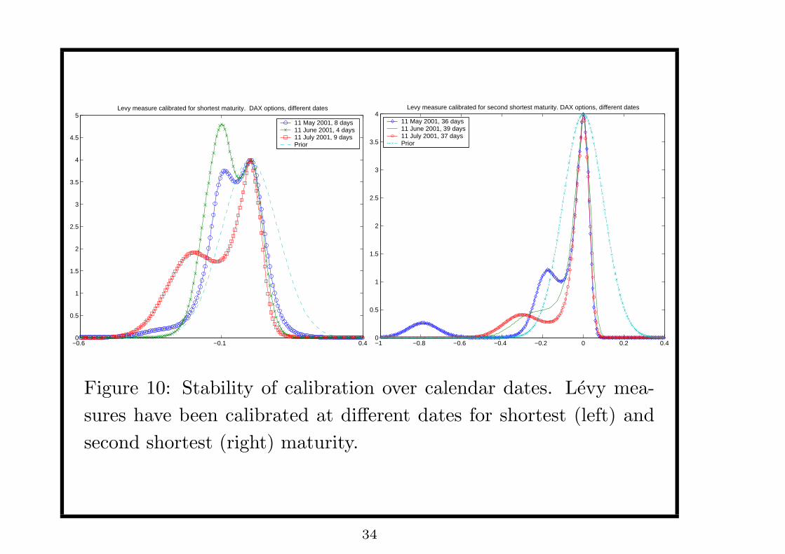
Figure 10: Stability of calibration over calendar dates. Levy mea-

sures have been calibrated at different dates for shortest (left) and

second shortest (right) maturity.

34

5000

5500

6000

6500

7000 0

0.2

0.4

0.6

0.8

1

0.16

0.18

0.2

0.22

0.24

0.26

0.28

0.3

Maturity

Market implied volatility surface, DAX options

Strike

Impl

ied

vola

tility

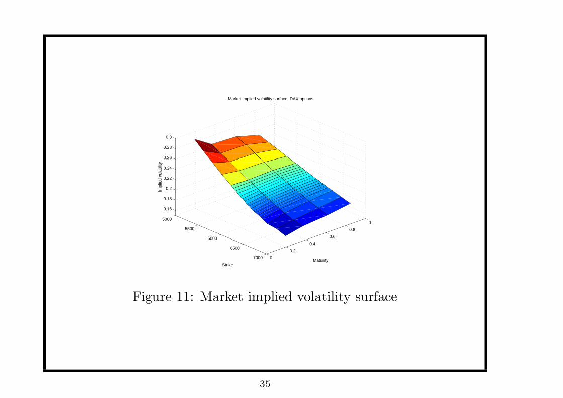
Figure 11: Market implied volatility surface

35

5000

5500

6000

6500

7000 00.2

0.40.6

0.81

0.15

0.2

0.25

0.3

Maturity

Levy measure calibrated to first maturity, DAX options.

Strike

Impl

ied

vola

tility

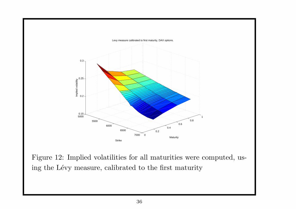
Figure 12: Implied volatilities for all maturities were computed, us-

ing the Levy measure, calibrated to the first maturity

36

5000

5500

6000

6500

7000 0

0.2

0.4

0.6

0.8

1

0.16

0.18

0.2

0.22

0.24

0.26

0.28

0.3

Maturity

Levy measure calibrated to last maturity, DAX options.

Strike

Impl

ied

vola

tility

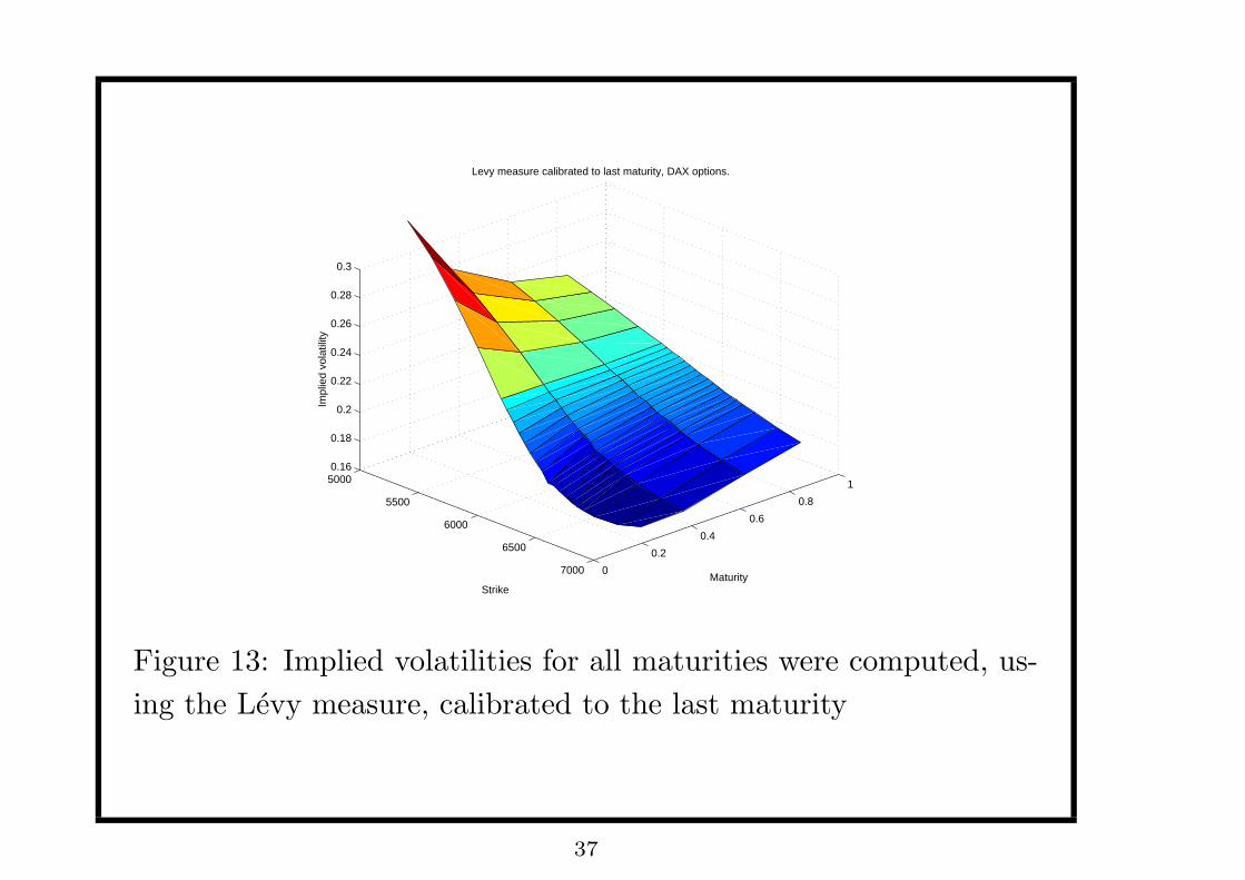
Figure 13: Implied volatilities for all maturities were computed, us-

ing the Levy measure, calibrated to the last maturity

37

Conclusion

We have proposed a non-parametric method for identifying risk

neutral jump-diffusion models consistent with market prices of

options and equivalent to a prespecified prior + a stable numerical

algorithm for computing it.

Theoretically : an extension of pricing using minimal entropy

martingale measure made consistent with observed market prices of

options.

Computationally, it is a stable version of current least squares

calibration methods for Levy models which does not assume shape

restrictions on the Levy measure.

Time-inhomogeneities can be easily incorporated into the

framework.

38

Applications and Extensions

• Specification tests for parametric exp Levy models.

• Identification of interesting parametric classes of Levy

measures from options data.

• Investigation of appropriate time-inhomogeneous extensions.

• Calibration of mixed jump diffusion/ stochastic volatility

models.

• Calibration of reduced form/ hybrid credit risk models.

• Multivariate jump diffusion models.

39