non-linear feature identifications based on self-sensing impedance measurements for structural...

ARTICLE IN PRESS

Mechanical Systemsand

Signal Processing

0888-3270/$ - se

doi:10.1016/j.ym

�CorrespondE-mail addr

Mechanical Systems and Signal Processing 21 (2007) 322–333

www.elsevier.com/locate/jnlabr/ymssp

Non-linear feature identifications based on self-sensingimpedance measurements for structural health assessment

Amanda C. Rutherford, Gyuhae Park�, Charles R. Farrar

Los Alamos National Laboratory, Engineering Sciences & Applications, The Engineering Institute, Mail Stop T001,

Weapon Response Group, Los Alamos, NM 87545, USA

Received 10 January 2005; received in revised form 6 October 2005; accepted 18 October 2005

Available online 28 November 2005

Abstract

This paper presents the application of a non-linear feature identification technique for structural damage detection. This

method is coupled with the impedance-based structural health monitoring (SHM) method, which utilises electro-

mechanical coupling properties of piezoelectric materials. The non-linear feature examined in this study is in the form of

autoregressive coefficients in the frequency domain autoregressive model with exogenous (ARX) inputs, which explicitly

considers non-linear system input/output relationships. The applicability of this non-linear feature for damage

identification is investigated in various frequency ranges using impedance signals measured from a laboratory-test

structure. The performance of the non-linear feature is also compared with those of linear features typically used in

impedance methods. This paper reinforces the utility of non-linear features in SHM and suggests that their sensitivity in

different frequency ranges may be leveraged for certain applications.

Published by Elsevier Ltd.

Keywords: Structural health monitoring; Nonlinearity; Active-sensing; Impedance-based structural health monitoring

1. Introduction

The process of implementing a damage detection strategy for aerospace, civil, and mechanicalinfrastructures is referred to as structural health monitoring (SHM). Damage here is defined as changes tothe material and/or geometric properties of these systems, which adversely affects the current or futureperformance of the systems. The SHM process involves the observation of a system over time usingperiodically spaced dynamic response measurements, the extraction of damage sensitive features from thesemeasurements, and the statistical analysis of these features to determine the current state of system health.

Recently, the structural community has turned its attention to developing high-frequency, in-service damageidentification techniques that provide required sensitivity to localised, minor defects in a system. Piezoelectric(PZT) materials are particularly useful for this purpose because they can perform both duties of sensing and

e front matter Published by Elsevier Ltd.

ssp.2005.10.002

ing author. Tel.: +1 505 663 5335; fax: +1 505 663 5225.

ess: [email protected] (G. Park).

www.elsevier.com/locate/jnlabr/ymssp

ARTICLE IN PRESSA.C. Rutherford et al. / Mechanical Systems and Signal Processing 21 (2007) 322–333 323

actuation, or even self-sensing, within a local area of the structure. One example of documented success usingPZT wafers for SHM is impedance-based SHM methods [1].

It is a well-known fact that non-linear dynamic features of a structure are more sensitive to many commontypes of damage than the linear features. In many cases, damage causes a structure, which exhibitspredominantly stationary and linear dynamic response properties in its undamaged state, to exhibit non-stationary and non-linear responses. Common examples of such damage includes cracks or delaminations thatopen and close when the structure is subjected to normal operating environments and loose parts rattling orsliding against one another. Thus, it is believed that a damage detection scheme that seeks to use non-linearcharacteristics could enhance the damage classification capability.

In this paper, we experimentally investigated the performance of non-linear features in structure healthmonitoring. Contrary to most non-linear feature extraction methods, which lie in the low-frequency modal-analysis domain, the features examined in this study are measured at relatively high-frequency ranges with theuse of the impedance method. The non-linear features associated with the electro-mechanical impedancemeasurements are extracted using the frequency domain autoregressive model with exogenous inputs (ARX)model, which explicitly considers non-linear system input/output relationships [2]. The varying sensitivity ofthe extracted linear and non-linear features in different frequency ranges is also analysed.

The rest of this paper will involve the introduction of the impedance method and the frequency domainARX model, experiments conducted on a portal frame structure, extraction of linear and non-linear featuresin various frequency ranges, and qualitative comparison of features.

2. Impedance-based structural health monitoring

The impedance-based health monitoring technique was first proposed by Sun et al. [3] and has since beenapplied to a wide variety of structures as a promising tool for real-time structural damage assessments[1,4,5–10,11]. The basic concept of this approach is to monitor the variations in structural mechanicalimpedance caused by the onset of damage. Since structural mechanical impedance measurements are difficultto obtain, impedance methods utilise the electrical impedance of surface bonded piezoelectric materials, whichis directly related to the mechanical impedance of the host structure, and will be affected by the onset ofstructural damage. Through monitoring the measured electrical impedance and comparing it to a baselinemeasurement, one can qualitatively determine that structural damage has occurred or is imminent. In order toensure high sensitivity to incipient damage, the electrical impedance is measured at high frequencies (typicallygreater than 20 kHz). At such high frequencies, the wavelength of the excitation is small and is sensitiveenough to detect minor changes in structural integrity. More importantly, high-frequency (kHz) signalsrequire very low voltage (less than 1V) to produce a useful impedance excitation in the host structure. Anotherkey aspect of the impedance-based methods is the use of PZT materials as a collocated sensor and actuator, inwhich only one PZT patch can be used for both actuation and sensing of the structural responses. The methodhas been proved to be effective for detecting various types of damage including corrosion and looseconnections. A complete description of the technique can be found in Refs. [1,7].

In SHM, the process of feature extraction is required for the selection of key information from the measureddata that distinguishes between a damaged and an undamaged structure. Feature extraction also accomplishesthe condensation of a large amount of available data into a much smaller data set that provides concisedamage indication. In impedance methods, the damage sensitive features traditionally employed are based onscalar damage metric, such as root mean square deviation (RMSD) or cross-correlation coefficients. In earlierwork [3], a simple statistical algorithm, based on frequency-by-frequency comparisons and referred to as‘‘RMSD’’ has been used,

M ¼Xn

i¼1

ffiffiffiffiffiffiffiffiffiffiffiffiffiffiffiffiffiffiffiffiffiffiffiffiffiffiffiffiffiffiffiffiffiffiffiffiffiffiffiffiffiffiffiffiffiReðZi;1Þ �ReðZi;2Þ� �2

ReðZi;1Þ� �2

vuut , (1)

where M represents the damage metric, Zi,1 is the impedance of the PZT patch measured at healthy conditions,and Zi,2 is the impedance for comparison with the baseline measurement at ith frequency. In an RMSDdamage metric chart, the greater numerical value of the metric, the larger the difference between the baseline

ARTICLE IN PRESSA.C. Rutherford et al. / Mechanical Systems and Signal Processing 21 (2007) 322–333324

and the impedance measurement of interest indicating the presence of damage in a structure. Considering thecapacitive nature of PZT materials, the imaginary part has large magnitude as compared to the real part andtends to play a dominant role in the overall magnitude, but has very low sensitivity to damage. Therefore, thereal part of the impedance is mainly used for monitoring purpose.

Another scalar damage metric, referred to as the ‘‘cross-correlation’’ metric, can also be used to interpretand quantify information from different data sets. The correlation coefficient between two impedance datasets determines the linear relationship between the two signatures

r ¼1

n� 1

Pni¼1ðReðZi;1Þ �ReðZ̄1ÞÞðReðZi;2Þ �ReðZ̄2ÞÞ

sZ1sZ2

, (2)

where r is the correlation coefficient, Zi,1 is the baseline FRF data and Zi,2 is the FRF data in question at ithfrequency, Z̄1 and Z̄2 are the means of the signals and the s terms are the standard deviations. Forconvenience, the feature examined is typically (1–r) in order to ensure that with increasing damage or changein structural integrity, the metric values also increase. This provides a metric chart that is consistent with othermetrics, such as RMSD, in which metric values increase when there is an increase in levels of damage. Thecross-correlation metric accounts for vertical and horizontal shifts of impedance signatures, usually associatedwith temperature changes. In most cases, the results with the correlation metric are consistent with thoseof RMSD.

The linear features described above are well suited to situations in which one structural state is to bediscriminated from another in a linear sense, but they would not be able to quantify any non-linear changes.Because the frequency ranges of impedance measurements are typically high, it is hypothesised that somestructural non-linearities will be captured in the measurement. Non-linearity in a structure could manifestitself in an impedance signal in a few different ways. Non-linearities often result in changes in amplitude, peakshifts, and peak shape changes. Non-linearity in a structure can result in changes in the impedance signaturewith changing input force levels. Non-linearities may also result in frequency response that is correlated toboth the input and the output at various frequencies. Therefore, in this paper, we examine the characteristicsof a non-linear feature derived from measured impedance signals and its applicability to SHM problems usingthe frequency domain ARX model, that is detailed in the next section.

3. Frequency domain autoregressive model with exogenous inputs

Frequency response is important in structural dynamics because it relates inputs and outputs of thestructure at various frequencies. Analysing these responses can lead to useful information regarding the healthof the structure. Conventional frequency response function (FRF) estimators are based on a linearityassumption for the system. Though global behaviours of many large-scale buildings can be approximated in alinear fashion, there are always local non-linearities within the structures. To explicitly consider this non-linearity, a frequency domain ARX inputs is used [2]. In a traditional time-series application, an ARX modelattempts to predict response at the current time point based on its own past time point responses, as well as thecurrent and past inputs to the system. A frequency domain ARX model attempts to predict the response at aparticular frequency based on the input at that frequency, as well as responses at surrounding frequencies. Theresponses at the surrounding frequencies are included as inputs to the model to account for subharmonics andsuperharmonics introduced to the system through non-linear feedback. More details on frequency domainanalysis of data using an ARX model can be found in Refs. [2,12].

There are many possible forms of the frequency domain ARX model, with each depending on how theeffects of subharmonics and superharmonics are to be considered. In this study, the effects of non-linearities inthe system are accounted for by using a first-order model, which is the simplest model available. This first-order ARX model in the frequency domain can be represented as follows:

Y ðkÞ ¼ BðkÞUðkÞ þ A1ðkÞY ðk � 1Þ þ A�1ðkÞY ðk þ 1Þ; k ¼ 2; 3; . . . ;Nf � 1, (3)

where Nf is the highest frequency value examined, Y(k) is the response at kth frequency, U(k) is the input atkth frequency, and Y(k– 1) and Y(k+1) are the responses at (k– 1)th and (k+1)th frequencies, respectively.


A1(k) and A�1(k) are the frequency domain autoregressive coefficients, and B(k) is the exogenous coefficient.While the exogenous coefficient describes the linear effects, the autoregressive coefficients describe any non-linear effects that may be present in the system. If one does not consider the autoregressive coefficients, Eq. (3)becomes traditional FRF estimates. Therefore, in this study, autoregressive coefficients are used tocharacterise the non-linear nature of damage state, and exogenous coefficients are used for the linear nature ofsuch states.

The unique contribution of this work is that it uses a non-linear feature identification technique in additionto traditional linear features of electrical impedance signals to detect and quantify the damage state ofstructures. The performance of the non-linear features, especially its enhanced sensitivity (to all types ofvariability), is compared to that of the linear features.

4. Experimental set-up and procedure

A bolt-jointed, moment-resisting, frame structure was used as a test-bed in this study, shown in Fig. 1. Thestructure consists of aluminum members connected using steel angle brackets and screws, with a simulatedrigid base. Two columns (6.35� 50.8� 304.8mm) are connected to the top beam (6.35� 50.8� 558.8mm)using the bolted joints tightened to 17Nm in the healthy condition. PZT patches (25.4� 25.4� 0.254mm)were mounted on the left side of the symmetric structure (Corner 2), with PZT 1 mounted on the column andPZT 2 mounted on the beam, as shown in Fig. 1.

In order to measure the electrical impedance of the PZT, a simple impedance measuring circuit is used [10].The voltage into the PZT patch is used as the output to the frequency domain ARX model and the voltageoutput from the PZT circuit, as seen in Fig. 2, is used as the input. These voltages are measured in the timedomain, which is different from the traditional impedance-based methods that only record data in thefrequency domain using a sine-sweep test. Vout is proportional to the output current of the PZT patch.Electrical impedance of the PZT patch is related to the measured input and output voltage of the PZT wafer

Fig. 1. The portal frame structure tested and PZT 2 installed on the top beam.

ARTICLE IN PRESS

Fig. 2. Diagram of PZT circuit indicating locations of measured voltages Vin and Vout.

Table 1

Test matrix for the frame structure

Tests Structural condition

Baseline Undamaged

Baseline 1 No change from baseline, measurement after 2 h

Baseline 2 Disassemble/reassemble the top beam


Baseline 4 No change from baseline 3, measurement after 12 h


D11 Loosen corner 1 bolt to 8.5Nm

D12 Hand tighten corner 1 bolt

Baseline 6 Retighten to 17Nm

D21 Loosen corner 2 bolt to 8.5Nm

D22 Hand tighten corner 2 bolt

A.C. Rutherford et al. / Mechanical Systems and Signal Processing 21 (2007) 322–333326

through the following equation:

Zp ¼V p

Ip

¼V in � Vout

Vout=R) Zp ¼ R

Vin

Vout� 1

� �. (4)

A commercial data acquisition system controlled from a laptop PC is used to digitise the voltage analogsignals. Time histories were sampled at a rate of 51.2 kHz, producing 32,768 time points. Although thetraditional impedance measurements are made at much higher frequency ranges, the current hardware limitsour ability to sample in the time domain at frequencies over 51.2 kHz. An amplified random signal (2.5V) wasused as the voltage input for the testing. The value 220O resistor was used to measure the impedance of thePZT patches.

Baseline measurements of a structure should seek to capture all types of variability that the structure mightbe subject to, which would not be attributed to damage, such as temperature effects. Previous experimentationon this portal frame structure performed by Aumann et al. [13] revealed that variability in the portal frame dueto assembly and disassembly is greater than variability introduced by environmental condition changes.Baseline measurements in this set of experiments attempts to capture, to some extent, typical environmentalvariability and assembly/disassembly variability by disassembling the top beam in order to establish a truedecision limit for damage indications. Therefore, a total of 6 baseline time histories were recorded for bothPZT patches, with conditions noted in Table 1. Four damage states were then introduced at two differentlocations by loosening the bolts at those locations to 8.5Nm and then to hand tight. After implementing the


damage, the time histories were again recorded from each PZT. The full test matrix, which was performedsequentially, is shown in Table 1.

All time history data are first standardised by subtracting the mean and dividing by the standard deviation,as in the following Eq. (5):

x̄ ¼x� ms

, (5)

where x is the original vector, x̄ the normalised vector, m the mean of the original vector, and s the standarddeviation of the original vector. This process is used so that the damage detection algorithm can distinguishbetween structural damage and operational variability [14]. Because Y(k) and U(k) in Eq. (3) are complexnumbers, the coefficients B(k), A1(k) and A�1(k) coefficients are also complex. Therefore, for each frequency k,

there are 6 unknown coefficients that must be determined. In order to estimate the ARX coefficients, multiplesets of data need to be recorded while the structure is in the same condition. Because only one 32,768-pointtime history is available for each condition, each time history is split up into 29 separate 4096-point blockswith 75% overlap. A Hanning window is applied to each block of data. A fast Fourier transform (FFT) is thenperformed on all data blocks in order to transfer the time history information into the frequency domain.There are 29 equations (from the 29 FFTs) and 6 unknown coefficients, for each frequency value k, that mustbe solved. B(k), A1(k) and A�1(k) in Eq. (4) are then determined by minimising the sum of the squared errorassociated with how well the ARX model in Eq. (4) describes the measured impedance data.

5. Analysis of linear and non-linear features from impedance data

Quantification of the differences between the baselines and the damage cases through application of linearand non-linear feature extraction methods is the subject of this section. While the structure exhibits globallinearity, it was hypothesised that non-linearities would be present in the data due to the contacting interfacesof the parts and differences in these interfaces introduced in assembly/disassembly of the top beam. Cross-correlation coefficients are calculated and used to assess the conditions of the structure. Cross correlations oflinear and non-linear coefficients were calculated between six baseline measurements and each tested case. Thefirst baseline is used as a ‘‘true’’ undamaged signature, to which all other measurement are compared.

5.1. Linear feature

The real parts of the linear coefficients for PZT 1 and PZT 2 are plotted in Fig. 3(a) and (b), respectively, inthe frequency range of 10–20 kHz. It should be noted that, in the impedance methods, only the real part is

1 1.2 1.4 1.6 1.8 240

42

44

46

48

50

52

54

56

58

60

Frequency (Hz)

Rea

l Par

t (O

hm)

1 1.2 1.4 1.6 1.8 2

x 104x 104

40

41

42

43

44

45

46

47

48

49

50

Frequency (Hz)

Rea

l Par

t (O

hm)

(b)(a)

Fig. 3. Baselines of linear coefficients. Six measurements are shown without label. A relatively large variation was observed in PZT 2: (a)

PZT 1; (b) PZT 2.


usually used for monitoring structures because it is more sensitive to structural damage than the imaginarypart [1]. Therefore, for the frequency ARX model, only the real part is used for the analysis. For PZT 1, evenafter the assembly/disassembly procedure, the impedance signatures are repeatable and show relatively smallchanges. The variation is anticipated to increase in PZT 2 because PZT 2 is installed on the top-beam (thecomponent that is disassembled and reassembled). Large baseline variations in PZT 2 can be observed. Thevariation in the signal due to damage needs to be greater than the baseline variations in order to be detectable.

Fig. 4 illustrates PZT 2’s baselines and signals that were measured after the damage at Corner 2 (D21, D22in Table 1). It is easy to see that qualitatively that damaged signals are quite different with the appearance ofnew peaks and shifts, especially at the higher frequency levels. With increasing levels of the damage, theimpedance variation also becomes more noticeable. The other results, i.e. PZT 1 for D21, D22 and PZT 2 forD11, D12, are similar. The size of the structure and relatively low impedance frequency range (10–20 kHz)employed limits the ability of the PZT patches to detect damage ‘‘locally’’. Both PZT patches show somesensitivity to damage at Corner 1 and Corner 2. The impedance frequency must be kept higher in order for thedamage to be localised, because then the PZT patches are sensitive to the damage in the near field and lesssensitive to changes in far field.

1 1.2 1.4 1.6 1.8 2

x 104

40

45

50

55

Frequency (Hz)

Rea

l Par

t (O

hm)

Rea

l Par

t (O

hm)

1 1.2 1.4 1.6 1.8 2

x 104

40

45

50

55

Frequency (Hz)(b)(a)

Fig. 4. PZT 2, Linear coefficients of baselines and damage at corner 2: (a) Baselines and D21 (8.5Nm); (b) baselines and D22 (hand

tightened).

base 1 base 2 base 3 base 4 base 5 D11 D12 base D21 D220

0.1

0.2

0.3

0.4

0.5

different testsbase 1 base 2 base 3 base 4 base 5 D11 D12 base D21 D22

different tests

1-C

C

0

0.1

0.2

0.3

0.4

0.5

0.6

0.7

1-C

C

(b)(a)

Fig. 5. Cross correlation damage metric chart of linear feature at 10–20kHz: (a) PZT 1; (b) PZT 2.


Quantification of damage was the next step. Results for PZT 1 and PZT 2 are shown in Figs. 5. Crosscorrelations confirm what was suspected upon initial observation of the signals. The frequency employed andsize of the structure limits the ability of the PZT patches to detect damage locally at Corner 1. However, thecross correlation of PZT 1 reveals that it may distinguish between the 8.5Nm case and the hand tighteneddamage cases. The extent and distance of damage is somewhat related to the coefficients values. The crosscorrelation of PZT 2 does not show the same characteristics. It shows relatively large variations compared toPZT1 and it is only able to distinguish between damaged and undamaged states of the portal frame. Thiscould be because of the close proximity of PZT2 to both of the damaged joints and its location on the topbeam that is being assembled and disassembled. It should be noted that the linear coefficients and theirchanges with induced damage follow essentially the same pattern of the traditional impedance signals, whichwere measured by the impedance analyser.

5.2. Non-linear feature

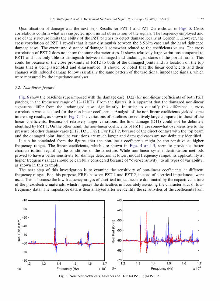
Fig. 6 show the baselines superimposed with the damage case (D22) for non-linear coefficients of both PZTpatches, in the frequency range of 12–17 kHz. From the figures, it is apparent that the damaged non-linearsignatures differ from the undamaged cases significantly. In order to quantify this difference, a crosscorrelation was calculated for the non-linear coefficients. Analysis of the non-linear coefficients yielded someinteresting results, as shown in Fig. 7. The variations of baselines are relatively large compared to those of thelinear coefficients. Because of relatively larger variations, the first damage (D11) could not be definitelyidentified by PZT 1. On the other hand, the non-linear coefficients of PZT 1 are somewhat over-sensitive to thepresence of other damage cases (D12, D21, D22). For PZT 2, because of the direct contact with the top beamand the damaged joint, baseline variations are much larger and damaged cases are not definitely identified.

It can be concluded from the figures that the non-linear coefficients might be too sensitive at higherfrequency ranges. The linear coefficients, which are shown in Figs. 4 and 5, seem to provide a bettercharacterisation regarding the conditions of the structure. While non-linear system identification methodsproved to have a better sensitivity for damage detection at lower, modal frequency ranges, its applicability athigher frequency ranges should be carefully considered because of ‘‘over-sensitivity’’ to all types of variability,as shown in this example.

The next step of this investigation is to examine the sensitivity of non-linear coefficients at differentfrequency ranges. For this purpose, FRFs between PZT 1 and PZT 2, instead of electrical impedances, wereused. This is because the low-frequency ranges of electrical impedance are dominated by the capacitive natureof the piezoelectric materials, which imposes the difficulties in accurately assessing the characteristics of low-frequency data. The impedance data is then analysed after we identify the sensitivities of the coefficients from

1.2 1.3 1.4 1.5 1.6 1.7

x 104

-80

-70

-60

-50

-40

-30

-20

-10

Frequency (Hz)

1.2 1.3 1.4 1.5 1.6 1.7

x 104Frequency (Hz)

Rea

l Par

t (O

hm)

-70

-65

-60

-55

-50

-45

-40

Rea

l Par

t (O

hm)

(b)(a)

Fig. 6. Nonlinear coefficients, baselines and D22: (a) PZT 1; (b) PZT 2.


the FRF measurements. The same experimental and analytical procedures are used as with the impedancemethod. As confirmed in the previous studies [1,15], the imaginary part of FRF is analogous to the real part ofthe electrical impedance (linear coefficients). Therefore, only the imaginary parts of FRF are examined, to beconsistent with the impedance analysis. Fig. 8 shows the imaginary part of the linear coefficients of the FRFbetween PZT1 and PZT2 with induced damage (D12).

The correlations were examined for linear and non-linear coefficients at two different frequency bands,0–2 kHz and 15–23 kHz as shown in Figs. 9 and 10. At lower frequency ranges, the linear coefficients could notdefinitively identify the small-scale damage cases (torque reduced to 8.5Nm), but the non-linear coefficientscould. In this case, the non-linear features increased sensitivity makes it superior to the linear features at lowerfrequency ranges, as confirmed by numerous studies [12,16]. At higher frequency ranges, however, the non-linear feature seems to be somewhat over-sensitive to baseline variations, and presence of damage is not asclear. On the other hand, the linear feature has much more baseline repeatability and improved sensitivity, andhence it can discriminate between baselines and all damage cases. These observations from FRF data confirm

1 1.2 1.4 1.6 1.8 2

x 104

-10

-8

-6

-4

-2

0

2

4

6

8

10

Frequency (Hz)

Imag

inar

y P

art (

V/V

)

Fig. 8. Linear coefficients from FRF between PZT1, baselines and D12.

0

0.1

0.2

0.3

0.4

0.5

0.6

0.7

0.8

0.9

1

1-C

C

1-C

C

0

0.1

0.2

0.3

0.4

0.5

0.6

0.7

0.8

0.9


different tests


different tests(b)(a)

Fig. 7. Correlation of non-linear coefficient, 10-20 kHz: (a) PZT 1; (b) PZT 2.

ARTICLE IN PRESS

0

0.1

0.2

0.3

0.4

0.5

0.6

0.7

0.1

0.2

0.3

0.4

0.5

0.6

0.7

0.8

0.9

1-C

C

1-C

C

0base 1 base 2 base 3 base 4 base 5 D11 D12 base D21 D22

different testsbase 1 base 2 base 3 base 4 base 5 D11 D12 base D21 D22


Fig. 9. Correlation of non-linear and linear coefficients, PZT 1-2 FRF, 0-2 kHz: (a) non-linear coefficient; (b) linear coefficient.

0

0.1

0.2

0.3

0.4

0.5

0.6

0.7

0.8

1-C

C

0

0.1

0.2

0.3

0.4

0.5

0.6

0.7

1-C

C


different tests



Fig. 10. Correlation of non-linear and linear coefficients, PZT 1-2 FRF, 15-23 kHz: (a) non-linear coefficient; (b) linear coefficient.

A.C. Rutherford et al. / Mechanical Systems and Signal Processing 21 (2007) 322–333 331

what has been observed in the previous studies combining non-linear features and impedance sensing. Basedon these results, the non-linear coefficients of the impedance data were once again analysed, but thistime in just the lower frequency ranges at 1–4 kHz. All damage cases could be successfully identified as shownin Fig. 11.

6. Discussion

It can be concluded from these observations that non-linear features, in the form of non-linear ARX modelcoefficients, demonstrated varying sensitivity to damage depending on the frequency range examined withincreased sensitivity (to all types of variability) at higher frequency ranges. Some other non-linear features,including reciprocity checks, changes in the magnitude of applied force (FRF distortions), and time-domainAR-ARX models, show the same kind of characteristics.

This quality of non-linear features could be leveraged in several ways, however. First, signal processingtechniques that capitalise on the increased sensitivity could be utilised. In this study, we only examined

ARTICLE IN PRESS

0

0.1

0.2

0.3

0.4

0.5

0.6

0.7

1-C

C

1-C

C

0

0.1

0.2

0.3

0.4

0.5

0.6

0.7

0.8

0.9


different tests



Fig. 11. Correlation of non-linear coefficients, PZT 1, 1-4 kHz: (a) PZT 1; (b) PZT 2.

A.C. Rutherford et al. / Mechanical Systems and Signal Processing 21 (2007) 322–333332

cross-correlation coefficients to assess the performance of the non-linear feature (and the RMSD showssimilar results). Other statistical feature extraction methods could be used in concert with the ARX non-linearcoefficients (such as moments, variance normalised coefficients, etc.) to utilise the improved sensitivity todamage and potentially decreasing baseline variability. Another desirable quality of the low-frequency rangesensitivity of the non-linear coefficients is that hardware sampling and data storage requirements could berelaxed. The changing sensitivity of non-linear features with frequency range could be leveraged for sensorlocations that are not ideal; i.e., sensors that are far field from damage could have increased sensitivity bylooking at non-linear coefficients for the higher frequency ranges. Finally, Because of the similarity betweenthe linear coefficients and the original impedance signals, the non-linear feature, especially in the form of thefrequency domain ARX model, could be used as supplementary information for the linear features. Thisapproach could result in confirmatory and somewhat redundant information for better performance in SHM.

7. Conclusions

Both linear and non-linear features of piezoelectric impedance are analysed for SHM applications. A seriesof experiments was performed on a portal frame. The linear feature shows an excellent capability at higherfrequency ranges. Non-linear features, in the form of non-linear ARX model coefficients, demonstratedvarying sensitivity to damage depending on the frequency range examined, with increased sensitivity (to alltypes of variability) at higher frequency ranges. This work further reinforces the utility of the use of non-linearfeatures for damage identification. Future work will include more investigation into binning of frequencyranges when using ARX coefficients, changing window size when fitting ARX models, looking at additionalstatistical feature extraction methods, and testing of more complex structures.

Acknowledgements

This research is funded through the Laboratory Directed Research and Development program, entitled‘‘Damage Prognosis Solution,’’ at Los Alamos National Laboratories.

References

[1] G. Park, H. Sohn, C.R. Farrar, D.J. Inman, Overview of piezoelectric impedance-based health monitoring and path forward, The

Shock and Vibration Digest 35 (6) (2003) 451–463.

[2] D.E. Adams, Frequency domain ARX models and multi-harmonic FRF estimators for nonlinear dynamic systems, Journal of Sound

and Vibration 250 (5) (2001) 935–950.


[3] F.P. Sun, Z. Chaudhry, C. Liang, C.A. Rogers, Truss structure integrity identification using PZT sensor-actuator, Journal of

Intelligent Material Systems and Structures 6 (1995) 134–139.

[4] V. Giurgiutiu, A.N. Zagrai, J.J. Bao, J.M. Redmond, D. Roach, K. Rackow, Active Sensors for health monitoring of aging aerospace

structures, International Journal of Condition Monitoring and Diagnostic Engineering Management 6 (1) (2003) 3–21.

[5] G. Mook, J. Pohl, M. Michel, Non-destructive characterization of smart CFRP structures, Smart Materials and Structures 12 (2003)

997–1004.

[6] K.K. Tseng, M.L. Tinker, J.O. Lassiter, D.M. Peairs, Temperature dependency of impedance-based nondestructive testing,

Experimental Techniques 27 (5) (2003) 33–36.

[7] S. Bhalla, C.K. Soh, Structural impedance-based damage diagnosis by piezo-transducers, Earthquake Engineering and Structural

Dynamics 32 (12) (2003) 1897–1916.

[8] S. Bhalla, C.K. Soh, High frequency piezoelectric signatures for diagnosis of seismic/blast induced structural damages, NDT&E

International 37 (1) (2004) 23–33.

[9] C. Bois, C. Hochard, Monitoring of laminated composites delamination based on electro-mechanical impedance measurement,

Journal of Intelligent Material Systems and Structures 15 (1) (2004) 59–67.

[10] D. Peairs, G. Park, D.J. Inman, Improving accessibility of the impedance-based structural health monitoring method, Journal of

Intelligent Material Systems and Structures 15 (2) (2004) 129–140.

[11] M. Abe, Y. Fujino, T. Miyashita, Quantitative health monitoring of bolted joints using a piezoceramic actuator-sensor, Smart

Materials and Structures 13 (1) (2004) 20–29.

[12] D.E. Adams, C.R. Farrar, Identifying linear and nonlinear damage using frequency domain ARX models, International Journal of

Structural Health Monitoring 1 (2) (2002) 185–201.

[13] R.J. Aumann, A.S. McCarty, C.C. Olson, Identification of random variation in structures and their parameter estimates. Proceedings

of the 22nd International Modal Analysis Conference, Society of Experimental Mechanics, Kissimmee, FL, 2003.

[14] H. Sohn, J.J. Czarnecki, C.R. Farrar, Structural health monitoring using statistical process control, ASCE Journal of Structural

Engineering 126 (11) (2000) 1356–1363.

[15] V. Giurgiutiu, A.N. Zagrai, Embedded self-sensing piezoelectric active sensors for online structural identification, ASME Journal of

Vibration and Acoustics 124 (1) (2002) 116–125.

[16] S.W. Doebling, C.R. Farrar, M.B. Prime, A summary review of vibration-based damage identification methods, The Shock and

Vibration Digest Journal 30 (1998) 91–105.

non-linear feature identifications based on self-sensing impedance measurements for structural...

Documents