non-convex optimization for machine learning - jain and kar · non-convex optimization for machine...
TRANSCRIPT
Non-convex Optimization for Machine Learning1
Prateek JainMicrosoft Research [email protected]
Purushottam KarIIT Kanpur
December 22, 2017
1The official publication is available from now publishers viahttp://dx.doi.org/10.1561/2200000058
arX
iv:1
712.
0789
7v1
[st
at.M
L]
21
Dec
201
7
The official publication is available from now publishers viahttp://dx.doi.org/10.1561/2200000058
Contents
Abstract 1
Preface 2
Mathematical Notation 6
I Introduction and Basic Tools 8
1 Introduction 91.1 Non-convex Optimization . . . . . . . . . . . . . . . . . . . . . . . . . . . . . . . 91.2 Motivation for Non-convex Optimization . . . . . . . . . . . . . . . . . . . . . . . 91.3 Examples of Non-Convex Optimization Problems . . . . . . . . . . . . . . . . . . 101.4 The Convex Relaxation Approach . . . . . . . . . . . . . . . . . . . . . . . . . . 131.5 The Non-Convex Optimization Approach . . . . . . . . . . . . . . . . . . . . . . 141.6 Organization and Scope . . . . . . . . . . . . . . . . . . . . . . . . . . . . . . . . 15
2 Mathematical Tools 162.1 Convex Analysis . . . . . . . . . . . . . . . . . . . . . . . . . . . . . . . . . . . . 162.2 Convex Projections . . . . . . . . . . . . . . . . . . . . . . . . . . . . . . . . . . . 182.3 Projected Gradient Descent . . . . . . . . . . . . . . . . . . . . . . . . . . . . . . 202.4 Convergence Guarantees for PGD . . . . . . . . . . . . . . . . . . . . . . . . . . . 20
2.4.1 Convergence with Bounded Gradient Convex Functions . . . . . . . . . . 202.4.2 Convergence with Strongly Convex and Smooth Functions . . . . . . . . . 22
2.5 Exercises . . . . . . . . . . . . . . . . . . . . . . . . . . . . . . . . . . . . . . . . 252.6 Bibliographic Notes . . . . . . . . . . . . . . . . . . . . . . . . . . . . . . . . . . . 25
II Non-convex Optimization Primitives 27
3 Non-Convex Projected Gradient Descent 283.1 Non-Convex Projections . . . . . . . . . . . . . . . . . . . . . . . . . . . . . . . . 28
3.1.1 Projecting into Sparse Vectors . . . . . . . . . . . . . . . . . . . . . . . . 293.1.2 Projecting into Low-rank Matrices . . . . . . . . . . . . . . . . . . . . . . 29
3.2 Restricted Strong Convexity and Smoothness . . . . . . . . . . . . . . . . . . . . 303.3 Generalized Projected Gradient Descent . . . . . . . . . . . . . . . . . . . . . . . 313.4 Exercises . . . . . . . . . . . . . . . . . . . . . . . . . . . . . . . . . . . . . . . . 33
ii
CONTENTS4 Alternating Minimization 35
4.1 Marginal Convexity and Other Properties . . . . . . . . . . . . . . . . . . . . . . 354.2 Generalized Alternating Minimization . . . . . . . . . . . . . . . . . . . . . . . . 374.3 A Convergence Guarantee for gAM for Convex Problems . . . . . . . . . . . . . . 394.4 A Convergence Guarantee for gAM under MSC/MSS . . . . . . . . . . . . . . . . 414.5 Exercises . . . . . . . . . . . . . . . . . . . . . . . . . . . . . . . . . . . . . . . . 434.6 Bibliographic Notes . . . . . . . . . . . . . . . . . . . . . . . . . . . . . . . . . . . 44
5 The EM Algorithm 455.1 A Primer in Probabilistic Machine Learning . . . . . . . . . . . . . . . . . . . . . 455.2 Problem Formulation . . . . . . . . . . . . . . . . . . . . . . . . . . . . . . . . . . 475.3 An Alternating Maximization Approach . . . . . . . . . . . . . . . . . . . . . . . 475.4 The EM Algorithm . . . . . . . . . . . . . . . . . . . . . . . . . . . . . . . . . . . 485.5 Implementing the E/M steps . . . . . . . . . . . . . . . . . . . . . . . . . . . . . 505.6 Motivating Applications . . . . . . . . . . . . . . . . . . . . . . . . . . . . . . . . 51
5.6.1 Gaussian Mixture Models . . . . . . . . . . . . . . . . . . . . . . . . . . . 515.6.2 Mixed Regression . . . . . . . . . . . . . . . . . . . . . . . . . . . . . . . . 52
5.7 A Monotonicity Guarantee for EM . . . . . . . . . . . . . . . . . . . . . . . . . . 555.8 Local Strong Concavity and Local Strong Smoothness . . . . . . . . . . . . . . . 565.9 A Local Convergence Guarantee for EM . . . . . . . . . . . . . . . . . . . . . . . 58
5.9.1 A Note on the Application of Convergence Guarantees . . . . . . . . . . . 595.10 Exercises . . . . . . . . . . . . . . . . . . . . . . . . . . . . . . . . . . . . . . . . 605.11 Bibliographic Notes . . . . . . . . . . . . . . . . . . . . . . . . . . . . . . . . . . . 61
6 Stochastic Optimization Techniques 626.1 Motivating Applications . . . . . . . . . . . . . . . . . . . . . . . . . . . . . . . . 636.2 Saddles and why they Proliferate . . . . . . . . . . . . . . . . . . . . . . . . . . . 646.3 The Strict Saddle Property . . . . . . . . . . . . . . . . . . . . . . . . . . . . . . 656.4 The Noisy Gradient Descent Algorithm . . . . . . . . . . . . . . . . . . . . . . . 666.5 A Local Convergence Guarantee for NGD . . . . . . . . . . . . . . . . . . . . . . 676.6 Constrained Optimization with Non-convex Objectives . . . . . . . . . . . . . . . 736.7 Application to Orthogonal Tensor Decomposition . . . . . . . . . . . . . . . . . . 756.8 Exercises . . . . . . . . . . . . . . . . . . . . . . . . . . . . . . . . . . . . . . . . 756.9 Bibliographic Notes . . . . . . . . . . . . . . . . . . . . . . . . . . . . . . . . . . . 76
III Applications 79
7 Sparse Recovery 807.1 Motivating Applications . . . . . . . . . . . . . . . . . . . . . . . . . . . . . . . . 807.2 Problem Formulation . . . . . . . . . . . . . . . . . . . . . . . . . . . . . . . . . . 827.3 Sparse Regression: Two Perspectives . . . . . . . . . . . . . . . . . . . . . . . . . 827.4 Sparse Recovery via Projected Gradient Descent . . . . . . . . . . . . . . . . . . 837.5 Restricted Isometry and Other Design Properties . . . . . . . . . . . . . . . . . . 847.6 Ensuring RIP and other Properties . . . . . . . . . . . . . . . . . . . . . . . . . . 857.7 A Sparse Recovery Guarantee for IHT . . . . . . . . . . . . . . . . . . . . . . . . 877.8 Other Popular Techniques for Sparse Recovery . . . . . . . . . . . . . . . . . . . 88
7.8.1 Pursuit Techniques . . . . . . . . . . . . . . . . . . . . . . . . . . . . . . . 887.8.2 Convex Relaxation Techniques for Sparse Recovery . . . . . . . . . . . . . 897.8.3 Non-convex Regularization Techniques . . . . . . . . . . . . . . . . . . . . 90
iii
CONTENTS7.8.4 Empirical Comparison . . . . . . . . . . . . . . . . . . . . . . . . . . . . . 91
7.9 Extensions . . . . . . . . . . . . . . . . . . . . . . . . . . . . . . . . . . . . . . . . 917.9.1 Sparse Recovery in Ill-Conditioned Settings . . . . . . . . . . . . . . . . . 927.9.2 Recovery from a Union of Subspaces . . . . . . . . . . . . . . . . . . . . . 927.9.3 Dictionary Learning . . . . . . . . . . . . . . . . . . . . . . . . . . . . . . 92
7.10 Exercises . . . . . . . . . . . . . . . . . . . . . . . . . . . . . . . . . . . . . . . . 937.11 Bibliographic Notes . . . . . . . . . . . . . . . . . . . . . . . . . . . . . . . . . . . 93
8 Low-rank Matrix Recovery 948.1 Motivating Applications . . . . . . . . . . . . . . . . . . . . . . . . . . . . . . . . 948.2 Problem Formulation . . . . . . . . . . . . . . . . . . . . . . . . . . . . . . . . . . 968.3 Matrix Design Properties . . . . . . . . . . . . . . . . . . . . . . . . . . . . . . . 97
8.3.1 The Matrix Restricted Isometry Property . . . . . . . . . . . . . . . . . . 978.3.2 The Matrix Incoherence Property . . . . . . . . . . . . . . . . . . . . . . . 97
8.4 Low-rank Matrix Recovery via Proj. Gradient Descent . . . . . . . . . . . . . . . 988.5 A Low-rank Matrix Recovery Guarantee for SVP . . . . . . . . . . . . . . . . . . 998.6 Matrix Completion via Alternating Minimization . . . . . . . . . . . . . . . . . . 1008.7 A Low-rank Matrix Completion Guarantee for AM-MC . . . . . . . . . . . . . . 1018.8 Other Popular Techniques for Matrix Recovery . . . . . . . . . . . . . . . . . . . 1058.9 Exercises . . . . . . . . . . . . . . . . . . . . . . . . . . . . . . . . . . . . . . . . 1068.10 Bibliographic Notes . . . . . . . . . . . . . . . . . . . . . . . . . . . . . . . . . . . 106
9 Robust Linear Regression 1089.1 Motivating Applications . . . . . . . . . . . . . . . . . . . . . . . . . . . . . . . . 1089.2 Problem Formulation . . . . . . . . . . . . . . . . . . . . . . . . . . . . . . . . . . 1109.3 Robust Regression via Alternating Minimization . . . . . . . . . . . . . . . . . . 1119.4 A Robust Recovery Guarantee for AM-RR . . . . . . . . . . . . . . . . . . . . . . 1129.5 Alternating Minimization via Gradient Updates . . . . . . . . . . . . . . . . . . . 1149.6 Robust Regression via Projected Gradient Descent . . . . . . . . . . . . . . . . . 1149.7 Empirical Comparison . . . . . . . . . . . . . . . . . . . . . . . . . . . . . . . . . 1159.8 Exercises . . . . . . . . . . . . . . . . . . . . . . . . . . . . . . . . . . . . . . . . 1169.9 Bibliographic Notes . . . . . . . . . . . . . . . . . . . . . . . . . . . . . . . . . . . 117
10 Phase Retrieval 11810.1 Motivating Applications . . . . . . . . . . . . . . . . . . . . . . . . . . . . . . . . 11810.2 Problem Formulation . . . . . . . . . . . . . . . . . . . . . . . . . . . . . . . . . . 11910.3 Phase Retrieval via Alternating Minimization . . . . . . . . . . . . . . . . . . . . 12010.4 A Phase Retrieval Guarantee for GSAM . . . . . . . . . . . . . . . . . . . . . . . 12110.5 Phase Retrieval via Gradient Descent . . . . . . . . . . . . . . . . . . . . . . . . 12210.6 A Phase Retrieval Guarantee for WF . . . . . . . . . . . . . . . . . . . . . . . . . 12310.7 Bibliographic Notes . . . . . . . . . . . . . . . . . . . . . . . . . . . . . . . . . . . 123
iv
The official publication is available from now publishers viahttp://dx.doi.org/10.1561/2200000058
List of Figures
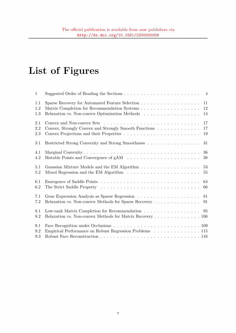
1 Suggested Order of Reading the Sections . . . . . . . . . . . . . . . . . . . . . . . 4
1.1 Sparse Recovery for Automated Feature Selection . . . . . . . . . . . . . . . . . . 111.2 Matrix Completion for Recommendation Systems . . . . . . . . . . . . . . . . . . 121.3 Relaxation vs. Non-convex Optimization Methods . . . . . . . . . . . . . . . . . 14
2.1 Convex and Non-convex Sets . . . . . . . . . . . . . . . . . . . . . . . . . . . . . 172.2 Convex, Strongly Convex and Strongly Smooth Functions . . . . . . . . . . . . . 172.3 Convex Projections and their Properties . . . . . . . . . . . . . . . . . . . . . . . 19
3.1 Restricted Strong Convexity and Strong Smoothness . . . . . . . . . . . . . . . . 31
4.1 Marginal Convexity . . . . . . . . . . . . . . . . . . . . . . . . . . . . . . . . . . . 364.2 Bistable Points and Convergence of gAM . . . . . . . . . . . . . . . . . . . . . . 38
5.1 Gaussian Mixture Models and the EM Algorithm . . . . . . . . . . . . . . . . . . 535.2 Mixed Regression and the EM Algorithm . . . . . . . . . . . . . . . . . . . . . . 55
6.1 Emergence of Saddle Points . . . . . . . . . . . . . . . . . . . . . . . . . . . . . . 646.2 The Strict Saddle Property . . . . . . . . . . . . . . . . . . . . . . . . . . . . . . 66
7.1 Gene Expression Analysis as Sparse Regression . . . . . . . . . . . . . . . . . . . 817.2 Relaxation vs. Non-convex Methods for Sparse Recovery . . . . . . . . . . . . . . 91
8.1 Low-rank Matrix Completion for Recommendation . . . . . . . . . . . . . . . . . 958.2 Relaxation vs. Non-convex Methods for Matrix Recovery . . . . . . . . . . . . . . 106
9.1 Face Recognition under Occlusions . . . . . . . . . . . . . . . . . . . . . . . . . . 1099.2 Empirical Performance on Robust Regression Problems . . . . . . . . . . . . . . 1159.3 Robust Face Reconstruction . . . . . . . . . . . . . . . . . . . . . . . . . . . . . . 116
v

The official publication is available from now publishers viahttp://dx.doi.org/10.1561/2200000058
List of Algorithms
1 Projected Gradient Descent (PGD) . . . . . . . . . . . . . . . . . . . . . . . . . . 202 Generalized Projected Gradient Descent (gPGD) . . . . . . . . . . . . . . . . . . 323 Generalized Alternating Minimization (gAM) . . . . . . . . . . . . . . . . . . . . 374 AltMax for Latent Variable Models (AM-LVM) . . . . . . . . . . . . . . . . . . . 475 Expectation Maximization (EM) . . . . . . . . . . . . . . . . . . . . . . . . . . . 506 Noisy Gradient Descent (NGD) . . . . . . . . . . . . . . . . . . . . . . . . . . . . 677 Projected Noisy Gradient Descent (PNGD) . . . . . . . . . . . . . . . . . . . . . 738 Iterative Hard-thresholding (IHT) . . . . . . . . . . . . . . . . . . . . . . . . . . 839 Singular Value Projection (SVP) . . . . . . . . . . . . . . . . . . . . . . . . . . . 9810 AltMin for Matrix Completion (AM-MC) . . . . . . . . . . . . . . . . . . . . . . 10011 AltMin for Robust Regression (AM-RR) . . . . . . . . . . . . . . . . . . . . . . . 11112 Gerchberg-Saxton Alternating Minimization (GSAM) . . . . . . . . . . . . . . . 12013 Wirtinger’s Flow for Phase Retrieval (WF) . . . . . . . . . . . . . . . . . . . . . 123
vi

The official publication is available from now publishers viahttp://dx.doi.org/10.1561/2200000058
Abstract
A vast majority of machine learning algorithms train their models and perform inference bysolving optimization problems. In order to capture the learning and prediction problems accu-rately, structural constraints such as sparsity or low rank are frequently imposed or else theobjective itself is designed to be a non-convex function. This is especially true of algorithmsthat operate in high-dimensional spaces or that train non-linear models such as tensor modelsand deep networks.
The freedom to express the learning problem as a non-convex optimization problem gives im-mense modeling power to the algorithm designer, but often such problems are NP-hard to solve.A popular workaround to this has been to relax non-convex problems to convex ones and usetraditional methods to solve the (convex) relaxed optimization problems. However this approachmay be lossy and nevertheless presents significant challenges for large scale optimization.
On the other hand, direct approaches to non-convex optimization have met with resoundingsuccess in several domains and remain the methods of choice for the practitioner, as they fre-quently outperform relaxation-based techniques – popular heuristics include projected gradientdescent and alternating minimization. However, these are often poorly understood in terms oftheir convergence and other properties.
This monograph presents a selection of recent advances that bridge a long-standing gapin our understanding of these heuristics. We hope that an insight into the inner workings ofthese methods will allow the reader to appreciate the unique marriage of task structure andgenerative models that allow these heuristic techniques to (provably) succeed. The monographwill lead the reader through several widely used non-convex optimization techniques, as well asapplications thereof. The goal of this monograph is to both, introduce the rich literature in thisarea, as well as equip the reader with the tools and techniques needed to analyze these simpleprocedures for non-convex problems.
1
The official publication is available from now publishers viahttp://dx.doi.org/10.1561/2200000058
Preface
Optimization as a field of study has permeated much of science and technology. The advent ofthe digital computer and a tremendous subsequent increase in our computational prowess hasincreased the impact of optimization in our lives. Today, tiny details such as airline schedules allthe way to leaps and strides in medicine, physics and artificial intelligence, all rely on modernadvances in optimization techniques.
For a large portion of this period of excitement, our energies were focused largely on con-vex optimization problems, given our deep understanding of the structural properties of convexsets and convex functions. However, modern applications in domains such as signal process-ing, bio-informatics and machine learning, are often dissatisfied with convex formulations alonesince there exist non-convex formulations that better capture the problem structure. For ap-plications in these domains, models trained using non-convex formulations often offer excellentperformance and other desirable properties such as compactness and reduced prediction times.
Examples of applications that benefit from non-convex optimization techniques include geneexpression analysis, recommendation systems, clustering, and outlier and anomaly detection. Inorder to get satisfactory solutions to these problems, that are scalable and accurate, we require adeeper understanding of non-convex optimization problems that naturally arise in these problemsettings.
Such an understanding was lacking until very recently and non-convex optimization foundlittle attention as an active area of study, being regarded as intractable. Fortunately, a long lineof works have recently led areas such as computer science, signal processing, and statistics torealize that the general abhorrence to non-convex optimization problems hitherto practiced, wasmisled. These works demonstrated in a beautiful way, that although non-convex optimizationproblems do suffer from intractability in general, those that arise in natural settings such asmachine learning and signal processing, possess additional structure that allow the intractabilityresults to be circumvented.
The first of these works still religiously stuck to convex optimization as the method of choice,and instead, sought to show that certain classes of non-convex problems which possess suitableadditional structure as offered by natural instances of those problems, could be converted toconvex problems without any loss. More precisely, it was shown that the original non-convexproblem and the modified convex problem possessed a common optimum and thus, the solutionto the convex problem would automatically solve the non-convex problem as well! However,these approaches had a price to pay in terms of the time it took to solve these so-called relaxedconvex problems. In several instances, these relaxed problems, although not intractable to solve,were nevertheless challenging to solve, at large scales.
It took a second wave of still more recent results to usher in provable non-convex optimizationtechniques which abstained from relaxations, solved the non-convex problems in their nativeforms, and yet seemed to offer the same quality of results as relaxation methods did. These newerresults were accompanied with a newer realization that, for a wide range of applications such assparse recovery, matrix completion, robust learning among others, these direct techniques are
2
Prefacefaster, often by an order of magnitude or more, than relaxation-based techniques while offeringsolutions of similar accuracy.
This monograph wishes to tell the story of this realization and the wisdom we gained from itfrom the point of view of machine learning and signal processing applications. The monographwill introduce the reader to a lively world of non-convex optimization problems with richstructure that can be exploited to obtain extremely scalable solutions to these problems. Put abit more dramatically, it will seek to show how problems that were once avoided, having beenshown to be NP-hard to solve, now have solvers that operate in near-linear time, by carefullyanalyzing and exploiting additional task structure! It will seek to inform the reader on how tolook for such structure in diverse application areas, as well as equip the reader with a soundbackground in fundamental tools and concepts required to analyze such problem areas andcome up with newer solutions.
How to use this monograph We have made efforts to make this monograph as self-containedas possible while not losing focus of the main topic of non-convex optimization techniques.Consequently, we have devoted entire sections to present a tutorial-like treatment to basicconcepts in convex analysis and optimization, as well as their non-convex counterparts. Assuch, this monograph can be used for a semester-length course on the basics of non-convexoptimization with applications to machine learning.
On the other hand, it is also possible to cherry pick portions of the monograph, such thesection on sparse recovery, or the EM algorithm, for inclusion in a broader course. Severalcourses such as those in machine learning, optimization, and signal processing may benefit fromthe inclusion of such topics. However, we advise that relevant background sections (see Figure 1)be covered beforehand.
While striving for breadth, the limits of space have constrained us from looking at sometopics in much detail. Examples include the construction of design matrices that satisfy theRIP/RSC properties and pursuit style methods, but there are several others. However, for allsuch omissions, the bibliographic notes at the end of each section can always be consultedfor references to details of the omitted topics. We have also been unable to address severalapplication areas such as dictionary learning, advances in low-rank tensor decompositions, topicmodeling and community detection in graphs but have provided pointers to prominent worksin these application areas too.
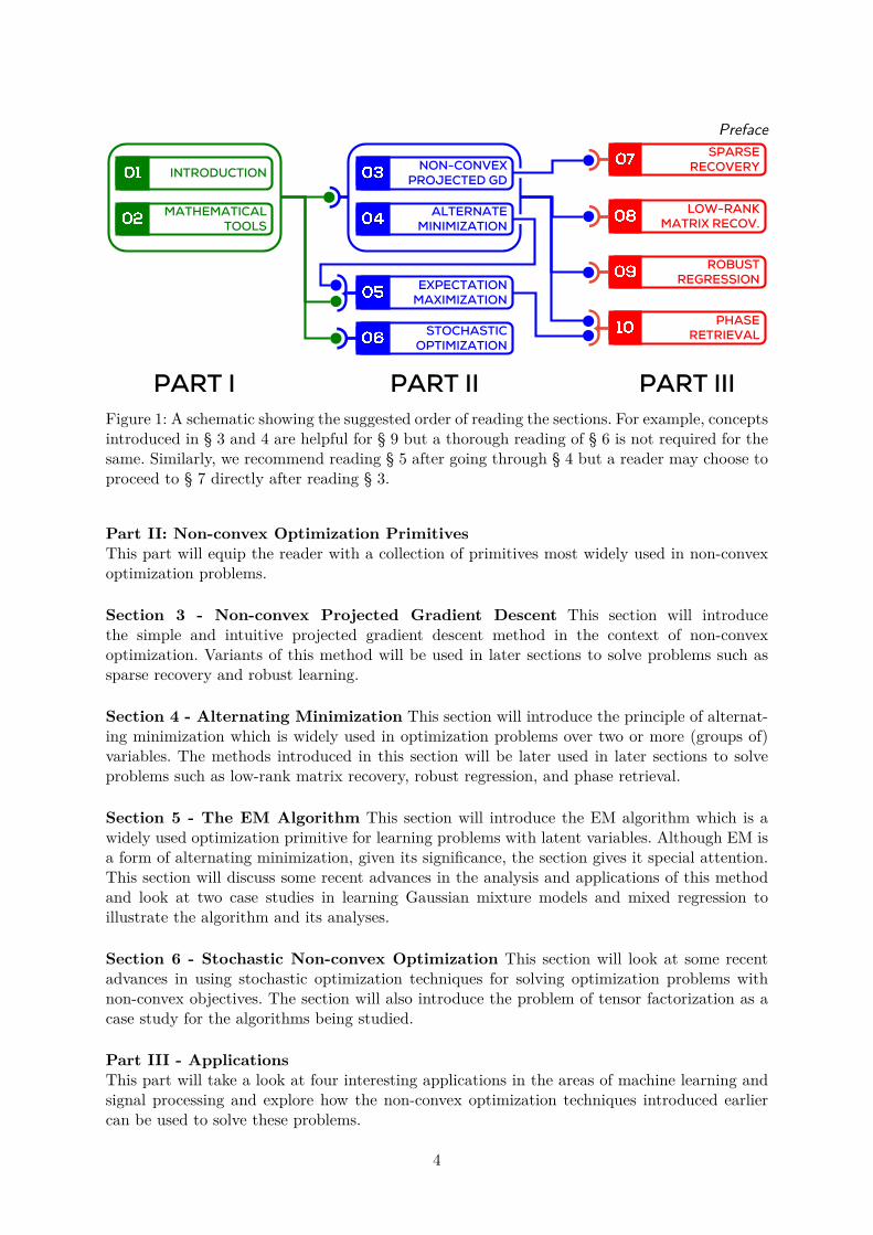
The organization of this monograph is outlined below with Figure 1 presenting a suggestedorder of reading the various sections.
Part I: Introduction and Basic ToolsThis part will offer an introductory note and a section exploring some basic definitions andalgorithmic tools in convex optimization. These sections are recommended to readers notintimately familiar with basics of numerical optimization.
Section 1 - Introduction This section will give a more relaxed introduction to the areaof non-convex optimization by discussing applications that motivate the use of non-convexformulations. The discussion will also clarify the scope of this monograph.
Section 2 - Mathematical Tools This section will set up notation and introduce some basicmathematical tools in convex optimization. This section is basically a handy repository of usefulconcepts and results and can be skipped by a reader familiar with them. Parts of the sectionmay instead be referred back to, as and when needed, using the cross-referencing links in themonograph.
3
Preface
INTRODUCTION
MATHEMATICAL TOOLS
SPARSERECOVERY
LOW-RANKMATRIX RECOV.
ROBUSTREGRESSION
PHASERETRIEVAL
NON-CONVEXPROJECTED GD
ALTERNATE MINIMIZATION
STOCHASTIC OPTIMIZATION
PART I PART II PART III
EXPECTATION MAXIMIZATION
Figure 1: A schematic showing the suggested order of reading the sections. For example, conceptsintroduced in § 3 and 4 are helpful for § 9 but a thorough reading of § 6 is not required for thesame. Similarly, we recommend reading § 5 after going through § 4 but a reader may choose toproceed to § 7 directly after reading § 3.
Part II: Non-convex Optimization PrimitivesThis part will equip the reader with a collection of primitives most widely used in non-convexoptimization problems.
Section 3 - Non-convex Projected Gradient Descent This section will introducethe simple and intuitive projected gradient descent method in the context of non-convexoptimization. Variants of this method will be used in later sections to solve problems such assparse recovery and robust learning.
Section 4 - Alternating Minimization This section will introduce the principle of alternat-ing minimization which is widely used in optimization problems over two or more (groups of)variables. The methods introduced in this section will be later used in later sections to solveproblems such as low-rank matrix recovery, robust regression, and phase retrieval.
Section 5 - The EM Algorithm This section will introduce the EM algorithm which is awidely used optimization primitive for learning problems with latent variables. Although EM isa form of alternating minimization, given its significance, the section gives it special attention.This section will discuss some recent advances in the analysis and applications of this methodand look at two case studies in learning Gaussian mixture models and mixed regression toillustrate the algorithm and its analyses.
Section 6 - Stochastic Non-convex Optimization This section will look at some recentadvances in using stochastic optimization techniques for solving optimization problems withnon-convex objectives. The section will also introduce the problem of tensor factorization as acase study for the algorithms being studied.
Part III - ApplicationsThis part will take a look at four interesting applications in the areas of machine learning andsignal processing and explore how the non-convex optimization techniques introduced earliercan be used to solve these problems.
4

PrefaceSection 7 - Sparse Recovery This section will look at a very basic non-convex optimizationproblem, that of performing linear regression to fit a sparse model to the data. The sectionwill discuss conditions under which it is possible to do so in polynomial time and show howthe non-convex projected gradient descent method studied earlier can be used to offer provablyoptimal solutions. The section will also point to other techniques used to solve this problem,as well as refer to extensions and related results.
Section 8 - Low-rank Matrix Recovery This section will address the more general problemof low rank matrix recovery with specific emphasis on low-rank matrix completion. The sectionwill gently introduce low-rank matrix recovery as a generalization of sparse linear regressionthat was studied in the previous section and then move on to look at matrix completion in moredetail. The section will apply both the non-convex projected gradient descent and alternatingminimization methods in the context of low-rank matrix recovery, analyzing simple cases andpointing to relevant literature.
Section 9 - Robust Regression This section will look at a widely studied area of machinelearning, namely robust learning, from the point of view of regression. Algorithms that arerobust to (adversarial) corruption in data are sought after in several areas of signal processingand learning. The section will explore how to use the projected gradient and alternatingminimization techniques to solve the robust regression problem and also look at applicationsof robust regression to robust face recognition and robust time series analysis.
Section 10 - Phase Retrieval This section will look at some recent advances in theapplication of non-convex optimization to phase retrieval. This problem lies at the heartof several imaging techniques such as X-ray crystallography and electron microscopy. A lotremains to be understood about this problem and existing algorithms often struggle to copewith the retrieval problems presented in practice.
The area of non-convex optimization has considerably widened in both scope and applicationin recent years and newer methods and analyses are being proposed at a rapid pace. While thismakes researchers working in this area extremely happy, it also makes summarizing the vastbody of work in a monograph such as this, more challenging. We have striven to strike a balancebetween presenting results that are the best known, and presenting them in a manner accessibleto a newcomer. However, in all cases, the bibliography notes at the end of each section docontain pointers to the state of the art in that area and can be referenced for follow-up readings.
Prateek Jain, Bangalore, IndiaPurushottam Kar, Kanpur, IndiaDecember 22, 2017
5
The official publication is available from now publishers viahttp://dx.doi.org/10.1561/2200000058
Mathematical Notation
• The set of real numbers is denoted by R. The set of natural numbers is denoted by N.
• The cardinality of a set S is denoted by |S|.
• Vectors are denoted by boldface, lower case alphabets for example, x,y. The zero vectoris denoted by 0. A vector x ∈ Rp will be in column format. The transpose of a vector isdenoted by x>. The ith coordinate of a vector x is denoted by xi.
• Matrices are denoted by upper case alphabets for example, A,B. Ai denotes the ith columnof the matrix A and Aj denotes its jth row. Aij denotes the element at the ith row andjth column.
• For a vector x ∈ Rp and a set S ⊂ [p], the notation xS denotes the vector z ∈ Rp suchthat zi = xi for i ∈ S, and zi = 0 otherwise. Similarly for matrices, AS denotes the matrixB with Bi = Ai for i ∈ S and Bi = 0 for i 6= S. Also, AS denotes the matrix B withBi = Ai for i ∈ S and Bi = 0> for i 6= S.
• The support of a vector x is denoted by supp(x) := i : xi 6= 0. A vector x is referred toas s-sparse if |supp(x)| ≤ s.
• The canonical directions in Rp are denoted by ei, i = 1, . . . , p.
• The identity matrix of order p is denoted by Ip×p or simply Ip. The subscript may beomitted when the order is clear from context.
• For a vector x ∈ Rp, the notation ‖x‖q = q√∑p
i=1 |xi|q denotes its Lq norm. As special
cases we define ‖x‖∞ := maxi |xi|, ‖x‖−∞ := mini |xi|, and ‖x‖0 := |supp(x)|.
• Balls with respect to various norms are denoted as Bq(r) :=
x ∈ Rp, ‖x‖q ≤ r. As a
special case the notation B0(s) is used to denote the set of s-sparse vectors.
• For a matrix A ∈ Rm×n, σ1(A) ≥ σ2(A) ≥ . . . ≥ σminm,n(A) denote its singular values.The Frobenius norm of A is defined as ‖A‖F :=
√∑i,j A
2ij =
√∑i σi(A)2. The nuclear
norm of A is defined as ‖A‖∗ :=∑i σi(A).
• The trace of a square matrix A ∈ Rm×m is defined as tr(A) =∑mi=1Aii.
• The spectral norm (also referred to as the operator norm) of a matrix A is defined as‖A‖2 := maxi σi(A).
• Random variables are denoted using upper case letters such as X,Y .
6

Mathematical Notation• The expectation of a random variable X is denoted by E [X]. In cases where the dis-
tribution of X is to be made explicit, the notation EX∼D [X], or else simply ED [X], isused.
• Unif(X ) denotes the uniform distribution over a compact set X .
• The standard big-Oh notation is used to describe the asymptotic behavior of functions.The soft-Oh notation is employed to hide poly-logarithmic factors i.e., f = O (g) willimply f = O (g logc(g)) for some absolute constant c.
7

The official publication is available from now publishers viahttp://dx.doi.org/10.1561/2200000058
Part I
Introduction and Basic Tools
8
The official publication is available from now publishers viahttp://dx.doi.org/10.1561/2200000058
Chapter 1
Introduction
This section will set the stage for subsequent discussions by motivating some of the non-convexoptimization problems we will be studying using real life examples, as well as setting up notationfor the same.
1.1 Non-convex OptimizationThe generic form of an analytic optimization problem is the following
minx∈Rp
f(x)
s.t. x ∈ C,
where x is the variable of the problem, f : Rp → R is the objective function of the problem,and C ⊆ Rp is the constraint set of the problem. When used in a machine learning setting, theobjective function allows the algorithm designer to encode proper and expected behavior for themachine learning model, such as fitting well to training data with respect to some loss function,whereas the constraint allows restrictions on the model to be encoded, for instance, restrictionson model size.
An optimization problem is said to be convex if the objective is a convex function, aswell as the constraint set is a convex set. We refer the reader to § 2 for formal definitionsof these terms. An optimization problem that violates either one of these conditions, i.e., onethat has a non-convex objective, or a non-convex constraint set, or both, is called a non-convexoptimization problem. In this monograph, we will discuss non-convex optimization problemswith non-convex objectives and convex constraints (§ 4, 5, 6, and 8), as well as problems withnon-convex constraints but convex objectives (§ 3, 7, 9, 10, and 8). Such problems arise in a lotof application areas.
1.2 Motivation for Non-convex OptimizationModern applications frequently require learning algorithms to operate in extremely high dimen-sional spaces. Examples include web-scale document classification problems where n-gram-basedrepresentations can have dimensionalities in the millions or more, recommendation systems withmillions of items being recommended to millions of users, and signal processing tasks such as facerecognition and image processing and bio-informatics tasks such as splice and gene detection,all of which present similarly high dimensional data.
Dealing with such high dimensionalities necessitates the imposition of structural constraintson the learning models being estimated from data. Such constraints are not only helpful in
9
CHAPTER 1. INTRODUCTIONregularizing the learning problem, but often essential to prevent the problem from becomingill-posed. For example, suppose we know how a user rates some items and wish to infer howthis user would rate other items, possibly in order to inform future advertisement campaigns.To do so, it is essential to impose some structure on how a user’s ratings for one set of itemsinfluences ratings for other kinds of items. Without such structure, it becomes impossible toinfer any new user ratings. As we shall soon see, such structural constraints often turn out tobe non-convex.
In other applications, the natural objective of the learning task is a non-convex function.Common examples include training deep neural networks and tensor decomposition problems.Although non-convex objectives and constraints allow us to accurately model learning problems,they often present a formidable challenge to algorithm designers. This is because unlike convexoptimization, we do not possess a handy set of tools for solving non-convex problems. Severalnon-convex optimization problems are known to be NP-hard to solve. The situation is mademore bleak by a range of non-convex problems that are not only NP-hard to solve optimally,but NP-hard to solve approximately as well [Meka et al., 2008].
1.3 Examples of Non-Convex Optimization ProblemsBelow we present some areas where non-convex optimization problems arise naturally whendevising learning problems.
Sparse Regression The classical problem of linear regression seeks to recover a linear modelwhich can effectively predict a response variable as a linear function of covariates. For example,we may wish to predict the average expenditure of a household (the response) as a function of theeducation levels of the household members, their annual salaries and other relevant indicators(the covariates). The ability to do allows economic policy decisions to be more informed byrevealing, for instance, how does education level affect expenditure.
More formally, we are provided a set of n covariate/response pairs (x1, y1), . . . , (xn, yn)where xi ∈ Rp and yi ∈ R. The linear regression approach makes the modeling assumptionyi = x>i w∗ + ηi where w∗ ∈ Rp is the underlying linear model and ηi is some benign additivenoise. Using the data provided xi, yii=1,...,n, we wish to recover back the model w∗ as faithfullyas possible.
A popular way to recover w∗ is using the least squares formulation
w = arg minw∈Rp
n∑i=1
(yi − x>i w
)2.
The linear regression problem as well as the least squares estimator, are extremely well studiedand their behavior, precisely known. However, this age-old problem acquires new dimensions insituations where, either we expect only a few of the p features/covariates to be actually relevantto the problem but do not know their identity, or else are working in extremely data-starvedsettings i.e., n p.
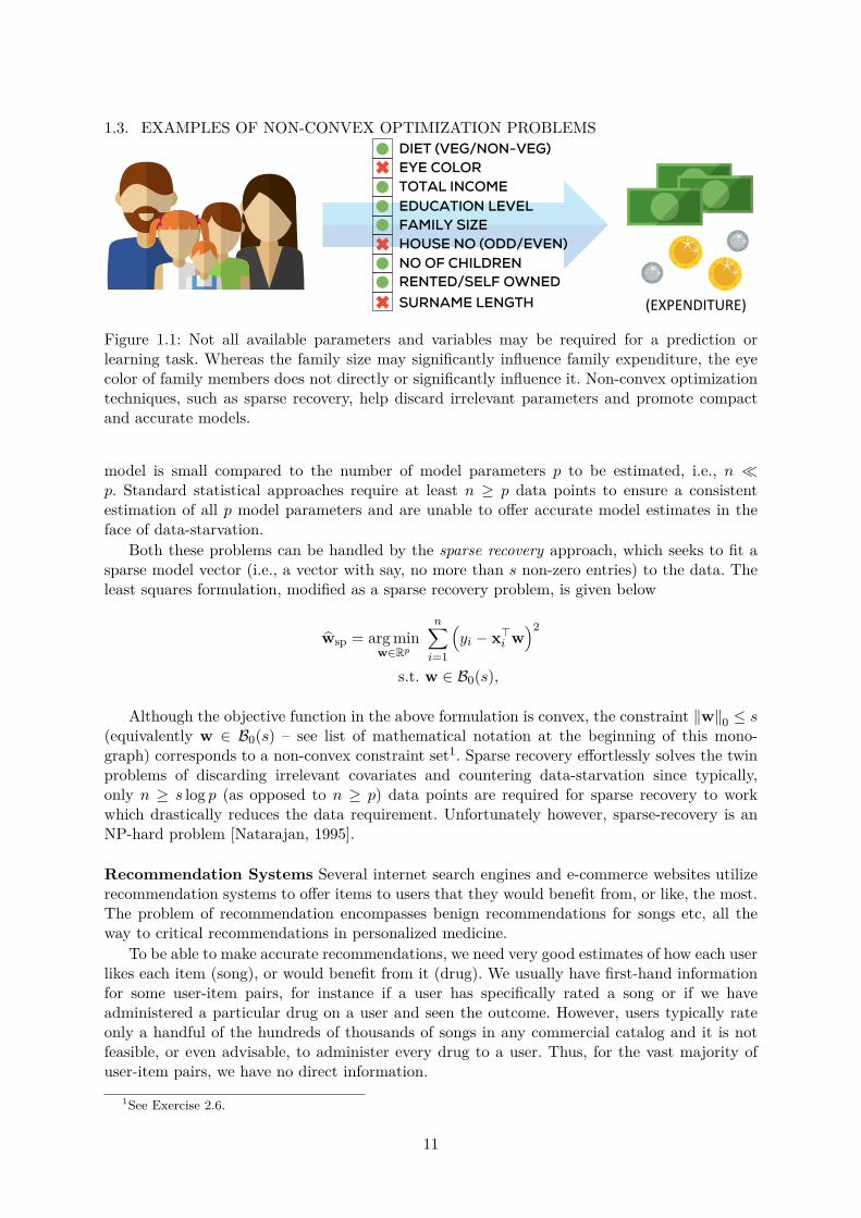
The first problem often arises when there is an excess of covariates, several of which maybe spurious or have no effect on the response. § 7 discusses several such practical examples. Fornow, consider the example depicted in Figure 1.1, that of expenditure prediction in a situationwhen the list of indicators include irrelevant ones such as whether the family lives in an odd-numbered house or not, which should arguably have no effect on expenditure. It is useful toeliminate such variables from consideration to promote consistency of the learned model.
The second problem is common in areas such as genomics and signal processing which facemoderate to severe data starvation and the number of data points n available to estimate the
10
1.3. EXAMPLES OF NON-CONVEX OPTIMIZATION PROBLEMS
EDUCATION LEVEL
FAMILY SIZE
TOTAL INCOME
HOUSE NO (ODD/EVEN)
RENTED/SELF OWNED
NO OF CHILDREN
SURNAME LENGTH
EYE COLOR
DIET (VEG/NON-VEG)
(EXPENDITURE)
Figure 1.1: Not all available parameters and variables may be required for a prediction orlearning task. Whereas the family size may significantly influence family expenditure, the eyecolor of family members does not directly or significantly influence it. Non-convex optimizationtechniques, such as sparse recovery, help discard irrelevant parameters and promote compactand accurate models.
model is small compared to the number of model parameters p to be estimated, i.e., n p. Standard statistical approaches require at least n ≥ p data points to ensure a consistentestimation of all p model parameters and are unable to offer accurate model estimates in theface of data-starvation.
Both these problems can be handled by the sparse recovery approach, which seeks to fit asparse model vector (i.e., a vector with say, no more than s non-zero entries) to the data. Theleast squares formulation, modified as a sparse recovery problem, is given below
wsp = arg minw∈Rp
n∑i=1
(yi − x>i w
)2
s.t. w ∈ B0(s),
Although the objective function in the above formulation is convex, the constraint ‖w‖0 ≤ s(equivalently w ∈ B0(s) – see list of mathematical notation at the beginning of this mono-graph) corresponds to a non-convex constraint set1. Sparse recovery effortlessly solves the twinproblems of discarding irrelevant covariates and countering data-starvation since typically,only n ≥ s log p (as opposed to n ≥ p) data points are required for sparse recovery to workwhich drastically reduces the data requirement. Unfortunately however, sparse-recovery is anNP-hard problem [Natarajan, 1995].
Recommendation Systems Several internet search engines and e-commerce websites utilizerecommendation systems to offer items to users that they would benefit from, or like, the most.The problem of recommendation encompasses benign recommendations for songs etc, all theway to critical recommendations in personalized medicine.
To be able to make accurate recommendations, we need very good estimates of how each userlikes each item (song), or would benefit from it (drug). We usually have first-hand informationfor some user-item pairs, for instance if a user has specifically rated a song or if we haveadministered a particular drug on a user and seen the outcome. However, users typically rateonly a handful of the hundreds of thousands of songs in any commercial catalog and it is notfeasible, or even advisable, to administer every drug to a user. Thus, for the vast majority ofuser-item pairs, we have no direct information.
1See Exercise 2.6.
11
CHAPTER 1. INTRODUCTION
ITEM FEATURES
USER FEATURES
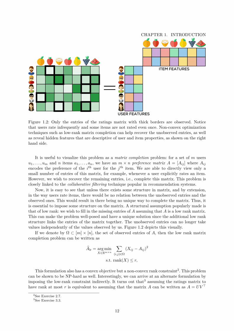
Figure 1.2: Only the entries of the ratings matrix with thick borders are observed. Noticethat users rate infrequently and some items are not rated even once. Non-convex optimizationtechniques such as low-rank matrix completion can help recover the unobserved entries, as wellas reveal hidden features that are descriptive of user and item properties, as shown on the righthand side.
It is useful to visualize this problem as a matrix completion problem: for a set of m usersu1, . . . , um and n items a1, . . . , an, we have an m × n preference matrix A = [Aij ] where Aijencodes the preference of the ith user for the jth item. We are able to directly view only asmall number of entries of this matrix, for example, whenever a user explicitly rates an item.However, we wish to recover the remaining entries, i.e., complete this matrix. This problem isclosely linked to the collaborative filtering technique popular in recommendation systems.
Now, it is easy to see that unless there exists some structure in matrix, and by extension,in the way users rate items, there would be no relation between the unobserved entries and theobserved ones. This would result in there being no unique way to complete the matrix. Thus, itis essential to impose some structure on the matrix. A structural assumption popularly made isthat of low rank: we wish to fill in the missing entries of A assuming that A is a low rank matrix.This can make the problem well-posed and have a unique solution since the additional low rankstructure links the entries of the matrix together. The unobserved entries can no longer takevalues independently of the values observed by us. Figure 1.2 depicts this visually.
If we denote by Ω ⊂ [m] × [n], the set of observed entries of A, then the low rank matrixcompletion problem can be written as
Alr = arg minX∈Rm×n
∑(i,j)∈Ω
(Xij −Aij)2
s.t. rank(X) ≤ r,
This formulation also has a convex objective but a non-convex rank constraint2. This problemcan be shown to be NP-hard as well. Interestingly, we can arrive at an alternate formulation byimposing the low-rank constraint indirectly. It turns out that3 assuming the ratings matrix tohave rank at most r is equivalent to assuming that the matrix A can be written as A = UV >
2See Exercise 2.7.3See Exercise 3.3.
12
1.4. THE CONVEX RELAXATION APPROACHwith the matrices U ∈ Rm×r and V ∈ Rn×r having at most r columns. This leads us to thefollowing alternate formulation
Alv = arg minU∈Rm×rV ∈Rn×r
∑(i,j)∈Ω
(U>i Vj −Aij
)2.
There are no constraints in the formulation. However, the formulation requires joint optimizationover a pair of variables (U, V ) instead of a single variable. More importantly, it can be shown4that the objective function is non-convex in (U, V ).
It is curious to note that the matrices U and V can be seen as encoding r-dimensionaldescriptions of users and items respectively. More precisely, for every user i ∈ [m], we canthink of the vector U i ∈ Rr (i.e., the i-th row of the matrix U) as describing user i, andfor every item j ∈ [n], use the row vector V j ∈ Rr to describe the item j in vectoralform. The rating given by user i to item j can now be seen to be Aij ≈
⟨U i, V j
⟩. Thus,
recovering the rank r matrix A also gives us a bunch of r-dimensional latent vectors de-scribing the users and items. These latent vectors can be extremely valuable in themselvesas they can help us in understanding user behavior and item popularity, as well as be usedin “content”-based recommendation systems which can effectively utilize item and user features.
The above examples, and several others from machine learning, such as low-rank tensordecomposition, training deep networks, and training structured models, demonstrate the util-ity of non-convex optimization in naturally modeling learning tasks. However, most of theseformulations are NP-hard to solve exactly, and sometimes even approximately. In the followingdiscussion, we will briefly introduce a few approaches, classical as well as contemporary, thatare used in solving such non-convex optimization problems.
1.4 The Convex Relaxation Approach
Faced with the challenge of non-convexity, and the associated NP-hardness, a traditionalworkaround in literature has been to modify the problem formulation itself so that existingtools can be readily applied. This is often done by relaxing the problem so that it becomes aconvex optimization problem. Since this allows familiar algorithmic techniques to be applied, theso-called convex relaxation approach has been widely studied. For instance, there exist relaxed,convex problem formulations for both the recommendation system and the sparse regressionproblems. For sparse linear regression, the relaxation approach gives us the popular LASSOformulation.
Now, in general, such modifications change the problem drastically, and the solutions of therelaxed formulation can be poor solutions to the original problem. However, it is known thatif the problem possesses certain nice structure, then under careful relaxation, these distortions,formally referred to as a“relaxation gap”, are absent, i.e., solutions to the relaxed problem wouldbe optimal for the original non-convex problem as well.
Although a popular and successful approach, this still has limitations, the most prominentof them being scalability. Although the relaxed convex optimization problems are solvable inpolynomial time, it is often challenging to solve them efficiently for large-scale problems.
4See Exercise 4.1.
13
CHAPTER 1. INTRODUCTION
DIMENSIONALITY
RU
NT
IME
(se
c) LASSO
FoBa
IHT
(a) Sparse Recovery (§ 7)
RU
NT
IME
(s
ec
) Ex. LASSO
AM-RR
gPGD
DATASET SIZE
(b) Robust Regression (§ 9)
RU
NT
IME
(s
ec
) SVT
SVP
SIZE OF MATRIX
(c) Matrix Recovery (§ 8)
SIZE OF MATRIX
RU
NT
IME
(se
c)
SVT
ADMiRA
SVP
(d) Matrix Completion (§ 8)
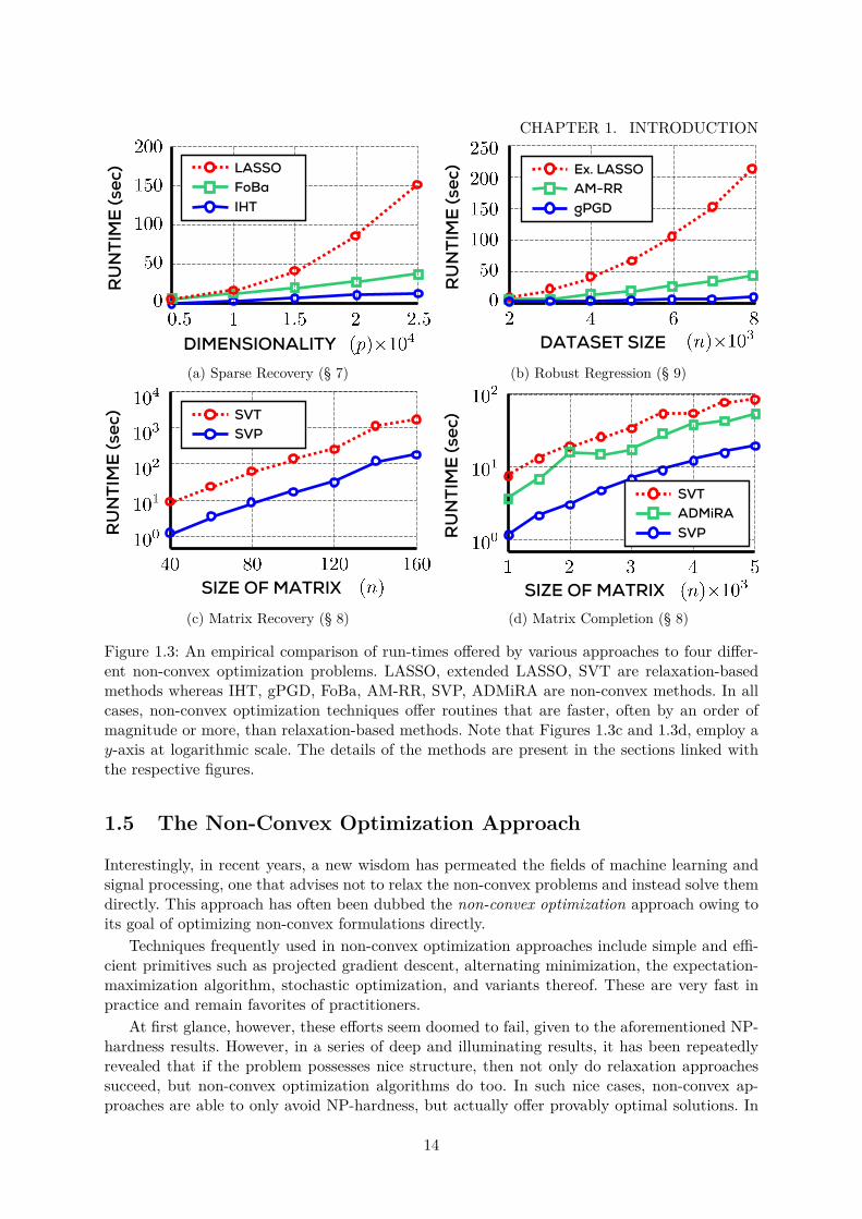
Figure 1.3: An empirical comparison of run-times offered by various approaches to four differ-ent non-convex optimization problems. LASSO, extended LASSO, SVT are relaxation-basedmethods whereas IHT, gPGD, FoBa, AM-RR, SVP, ADMiRA are non-convex methods. In allcases, non-convex optimization techniques offer routines that are faster, often by an order ofmagnitude or more, than relaxation-based methods. Note that Figures 1.3c and 1.3d, employ ay-axis at logarithmic scale. The details of the methods are present in the sections linked withthe respective figures.
1.5 The Non-Convex Optimization Approach
Interestingly, in recent years, a new wisdom has permeated the fields of machine learning andsignal processing, one that advises not to relax the non-convex problems and instead solve themdirectly. This approach has often been dubbed the non-convex optimization approach owing toits goal of optimizing non-convex formulations directly.
Techniques frequently used in non-convex optimization approaches include simple and effi-cient primitives such as projected gradient descent, alternating minimization, the expectation-maximization algorithm, stochastic optimization, and variants thereof. These are very fast inpractice and remain favorites of practitioners.
At first glance, however, these efforts seem doomed to fail, given to the aforementioned NP-hardness results. However, in a series of deep and illuminating results, it has been repeatedlyrevealed that if the problem possesses nice structure, then not only do relaxation approachessucceed, but non-convex optimization algorithms do too. In such nice cases, non-convex ap-proaches are able to only avoid NP-hardness, but actually offer provably optimal solutions. In
14

1.6. ORGANIZATION AND SCOPEfact, in practice, they often handsomely outperform relaxation-based approaches in terms ofspeed and scalability. Figure 1.3 illustrates this for some applications that we will investigatemore deeply in later sections.
Very interestingly, it turns out that problem structures that allow non-convex approachesto avoid NP-hardness results, are very similar to those that allow their convex relaxation coun-terparts to avoid distortions and a large relaxation gap! Thus, it seems that if the problemspossess nice structure, convex relaxation-based approaches, as well as non-convex techniques,both succeed. However, non-convex techniques usually offer more scalable solutions.
1.6 Organization and ScopeOur goal of this monograph is to present basic tools, both algorithmic and analytic, that arecommonly used in the design and analysis of non-convex optimization algorithms, as well aspresent results which best represent the non-convex optimization philosophy. The presentationshould enthuse, as well as equip, the interested reader and allow further readings, independentinvestigations, and applications of these techniques in diverse areas.
Given this broad aim, we shall appropriately restrict the number of areas we cover in thismonograph, as well as the depth in which we cover each area. For instance, the literatureabounds in results that seek to perform optimizations with more and more complex structuresbeing imposed - from sparse recovery to low rank matrix recovery to low rank tensor recovery.However, we shall restrict ourselves from venturing too far into these progressions. Similarly,within the problem of sparse recovery, there exist results for recovery in the simple least squaressetting, the more involved setting of sparse M-estimation, as well as the still more involvedsetting of sparse M-estimation in the presence of outliers. Whereas we will cover sparse leastsquares estimation in depth, we will refrain from delving too deeply into the more involvedsparse M-estimation problems.
That being said, the entire presentation will be self contained and accessible to anyone witha basic background in algebra and probability theory. Moreover, the bibliographic notes givenat the end of the sections will give pointers that should enable the reader to explore the stateof the art not covered in this monograph.
15
The official publication is available from now publishers viahttp://dx.doi.org/10.1561/2200000058
Chapter 2
Mathematical Tools
This section will introduce concepts, algorithmic tools, and analysis techniques used in thedesign and analysis of optimization algorithms. It will also explore simple convex optimizationproblems which will serve as a warm-up exercise.
2.1 Convex AnalysisWe recall some basic definitions in convex analysis. Studying these will help us appreciatethe structural properties of non-convex optimization problems later in the monograph. Forthe sake of simplicity, unless stated otherwise, we will assume that functions are continuouslydifferentiable. We begin with the notion of a convex combination.
Definition 2.1 (Convex Combination). A convex combination of a set of n vectors xi ∈ Rp,i = 1 . . . n in an arbitrary real space is a vector xθ :=
∑ni=1 θixi where θ = (θ1, θ2, . . . , θn),
θi ≥ 0 and∑ni=1 θi = 1.
A set that is closed under arbitrary convex combinations is a convex set. A standard defini-tion is given below. Geometrically speaking, convex sets are those that contain all line segmentsthat join two points inside the set. As a result, they cannot have any inward “bulges”.
Definition 2.2 (Convex Set). A set C ∈ Rp is considered convex if, for every x,y ∈ C andλ ∈ [0, 1], we have (1− λ) · x + λ · y ∈ C as well.
Figure 2.1 gives visual representations of prototypical convex and non-convex sets. A relatednotion is that of convex functions which have a unique behavior under convex combinations.There are several definitions of convex functions, those that are more basic and general, as wellas those that are restrictive but easier to use. One of the simplest definitions of convex functions,one that does not involve notions of derivatives, defines convex functions f : Rp → R as those forwhich, for every x,y ∈ Rp and every λ ∈ [0, 1], we have f((1−λ)·x+λ·y) ≤ (1−λ)·f(x)+λ·f(y).For continuously differentiable functions, a more usable definition follows.
Definition 2.3 (Convex Function). A continuously differentiable function f : Rp → R isconsidered convex if for every x,y ∈ Rp we have f(y) ≥ f(x) + 〈∇f(x),y− x〉, where ∇f(x)is the gradient of f at x.
A more general definition that extends to non-differentiable functions uses the notion ofsubgradient to replace the gradient in the above expression. A special class of convex functionsis the class of strongly convex and strongly smooth functions. These are critical to the study ofalgorithms for non-convex optimization. Figure 2.2 provides a handy visual representation ofthese classes of functions.
16
2.1. CONVEX ANALYSIS
CONVEX SET NON-CONVEX SET NON-CONVEX SET
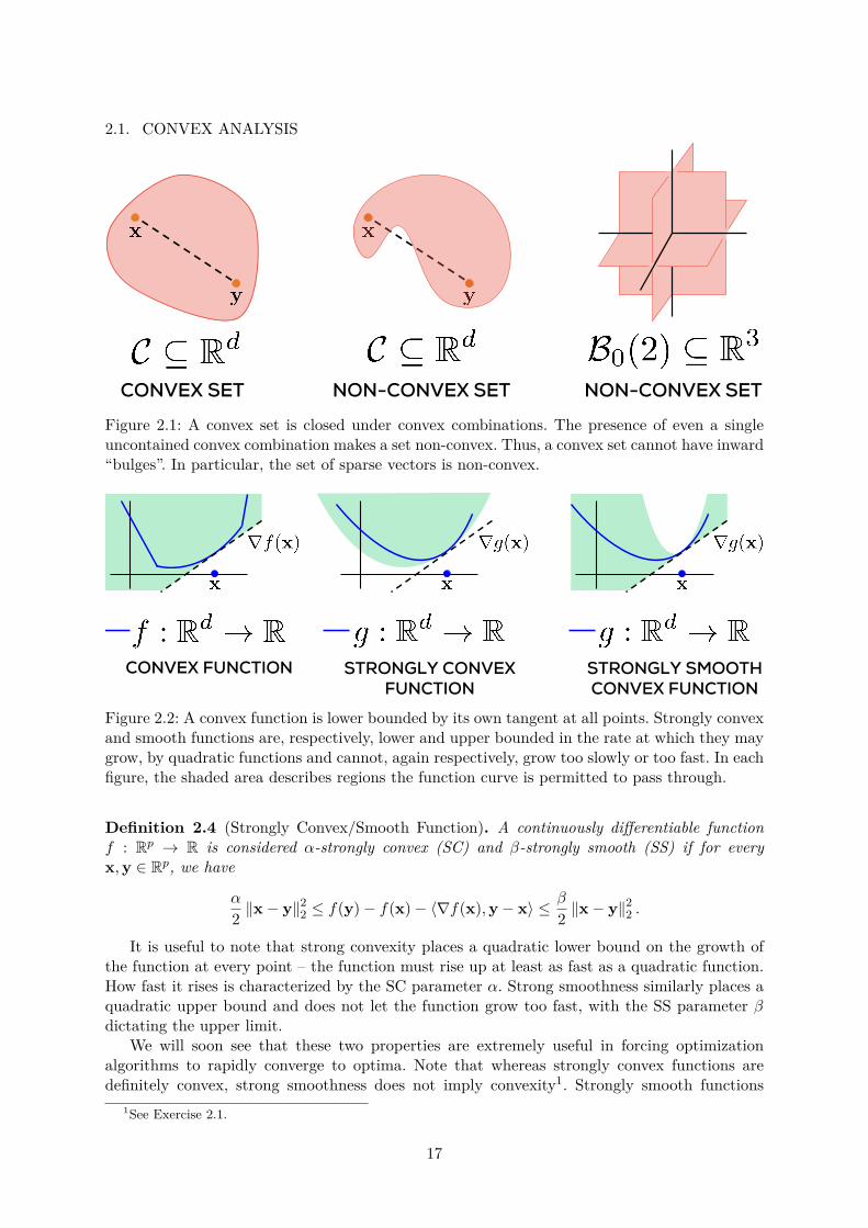
Figure 2.1: A convex set is closed under convex combinations. The presence of even a singleuncontained convex combination makes a set non-convex. Thus, a convex set cannot have inward“bulges”. In particular, the set of sparse vectors is non-convex.
STRONGLY SMOOTH CONVEX FUNCTION
CONVEX FUNCTION STRONGLY CONVEX FUNCTION
Figure 2.2: A convex function is lower bounded by its own tangent at all points. Strongly convexand smooth functions are, respectively, lower and upper bounded in the rate at which they maygrow, by quadratic functions and cannot, again respectively, grow too slowly or too fast. In eachfigure, the shaded area describes regions the function curve is permitted to pass through.
Definition 2.4 (Strongly Convex/Smooth Function). A continuously differentiable functionf : Rp → R is considered α-strongly convex (SC) and β-strongly smooth (SS) if for everyx,y ∈ Rp, we have
α
2 ‖x− y‖22 ≤ f(y)− f(x)− 〈∇f(x),y− x〉 ≤ β
2 ‖x− y‖22 .
It is useful to note that strong convexity places a quadratic lower bound on the growth ofthe function at every point – the function must rise up at least as fast as a quadratic function.How fast it rises is characterized by the SC parameter α. Strong smoothness similarly places aquadratic upper bound and does not let the function grow too fast, with the SS parameter βdictating the upper limit.
We will soon see that these two properties are extremely useful in forcing optimizationalgorithms to rapidly converge to optima. Note that whereas strongly convex functions aredefinitely convex, strong smoothness does not imply convexity1. Strongly smooth functions
1See Exercise 2.1.
17

CHAPTER 2. MATHEMATICAL TOOLSmay very well be non-convex. A property similar to strong smoothness is that of Lipschitznesswhich we define below.
Definition 2.5 (Lipschitz Function). A function f : Rp → R is B-Lipschitz if for every x,y ∈Rp, we have
|f(x)− f(y)| ≤ B · ‖x− y‖2 .
Notice that Lipschitzness places a upper bound on the growth of the function that is linearin the perturbation i.e., ‖x− y‖2, whereas strong smoothness (SS) places a quadratic upperbound. Also notice that Lipschitz functions need not be differentiable. However, differentiablefunctions with bounded gradients are always Lipschitz2. Finally, an important property thatgeneralizes the behavior of convex functions on convex combinations is the Jensen’s inequality.
Lemma 2.1 (Jensen’s Inequality). If X is a random variable taking values in the domain of aconvex function f , then E [f(X)] ≥ f(E [X])
This property will be useful while analyzing iterative algorithms.
2.2 Convex ProjectionsThe projected gradient descent technique is a popular method for constrained optimizationproblems, both convex as well as non-convex. The projection step plays an important role inthis technique. Given any closed set C ⊂ Rp, the projection operator ΠC(·) is defined as
ΠC(z) := arg minx∈C
‖x− z‖2 .
In general, one need not use only the L2-norm in defining projections but is the most commonlyused one. If C is a convex set, then the above problem reduces to a convex optimization problem.In several useful cases, one has access to a closed form solution for the projection.
For instance, if C = B2(1) i.e., the unit L2 ball, then projection is equivalent3 to a normal-ization step
ΠB2(1)(z) =
z/ ‖z‖2 if ‖z‖ > 1z otherwise
.
For the case C = B1(1), the projection step reduces to the popular soft thresholding operation.If z := ΠB1(1)(z), then zi = max zi − θ, 0, where θ is a threshold that can be decided by asorting operation on the vector [see Duchi et al., 2008, for details].
Projections onto convex sets have some very useful properties which come in handy whileanalyzing optimization algorithms. In the following, we will study three properties of projections.These are depicted visually in Figure 2.3 to help the reader gain an intuitive appeal.
Lemma 2.2 (Projection Property-O). For any set (convex or not) C ⊂ Rp and z ∈ Rp, letz := ΠC(z). Then for all x ∈ C, ‖z− z‖2 ≤ ‖x− z‖2.
This property follows by simply observing that the projection step solves the the optimizationproblem minx∈C ‖x− z‖2. Note that this property holds for all sets, whether convex or not.However, the following two properties necessarily hold only for convex sets.
Lemma 2.3 (Projection Property-I). For any convex set C ⊂ Rp and any z ∈ Rp, let z := ΠC(z).Then for all x ∈ C, 〈x− z, z− z〉 ≤ 0.
2See Exercise 2.2.3See Exercise 2.3.
18
2.2. CONVEX PROJECTIONS
PROJECTION PROPERTY O
PROJECTION PROPERTY I
PROJECTION PROPERTY II
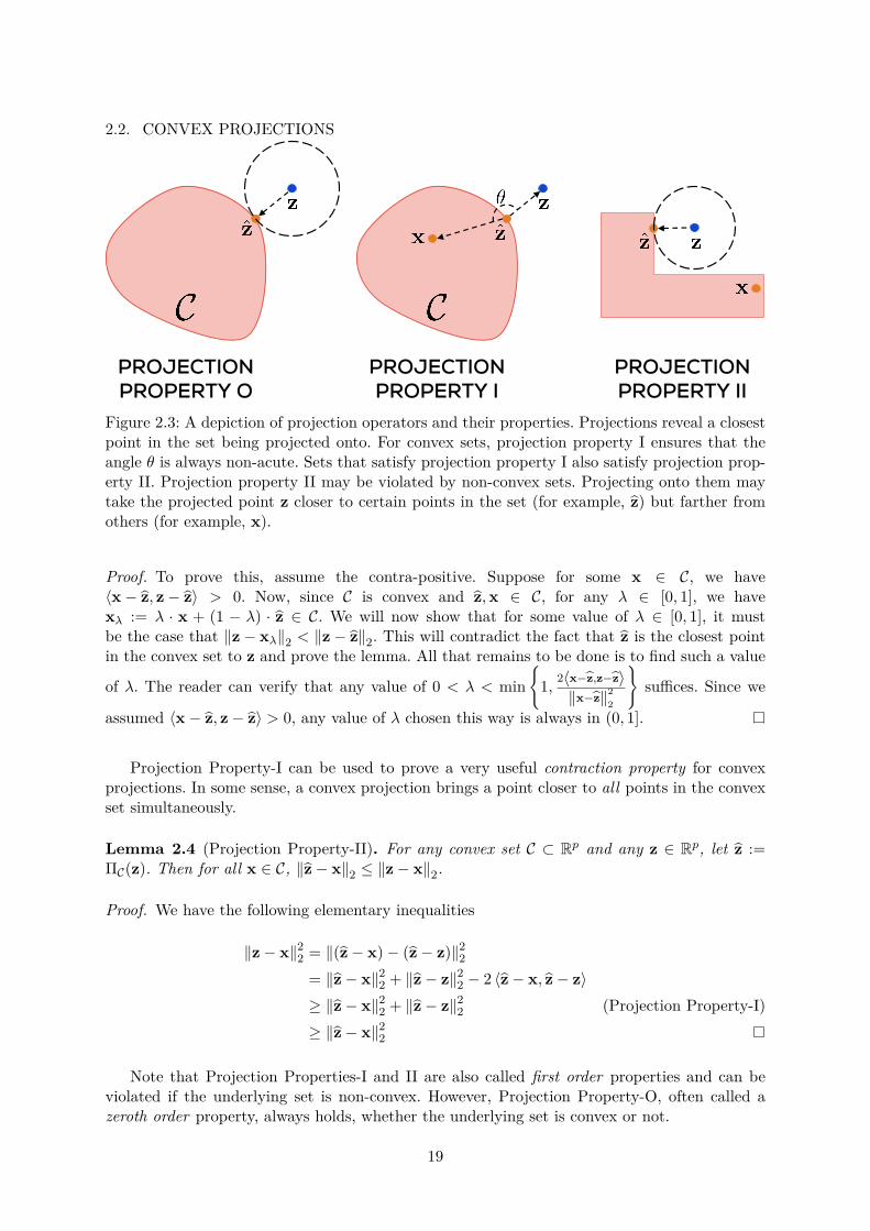
Figure 2.3: A depiction of projection operators and their properties. Projections reveal a closestpoint in the set being projected onto. For convex sets, projection property I ensures that theangle θ is always non-acute. Sets that satisfy projection property I also satisfy projection prop-erty II. Projection property II may be violated by non-convex sets. Projecting onto them maytake the projected point z closer to certain points in the set (for example, z) but farther fromothers (for example, x).
Proof. To prove this, assume the contra-positive. Suppose for some x ∈ C, we have〈x− z, z− z〉 > 0. Now, since C is convex and z,x ∈ C, for any λ ∈ [0, 1], we havexλ := λ · x + (1 − λ) · z ∈ C. We will now show that for some value of λ ∈ [0, 1], it mustbe the case that ‖z− xλ‖2 < ‖z− z‖2. This will contradict the fact that z is the closest pointin the convex set to z and prove the lemma. All that remains to be done is to find such a value
of λ. The reader can verify that any value of 0 < λ < min
1, 2〈x−z,z−z〉‖x−z‖2
2
suffices. Since we
assumed 〈x− z, z− z〉 > 0, any value of λ chosen this way is always in (0, 1].
Projection Property-I can be used to prove a very useful contraction property for convexprojections. In some sense, a convex projection brings a point closer to all points in the convexset simultaneously.
Lemma 2.4 (Projection Property-II). For any convex set C ⊂ Rp and any z ∈ Rp, let z :=ΠC(z). Then for all x ∈ C, ‖z− x‖2 ≤ ‖z− x‖2.
Proof. We have the following elementary inequalities
‖z− x‖22 = ‖(z− x)− (z− z)‖22= ‖z− x‖22 + ‖z− z‖22 − 2 〈z− x, z− z〉≥ ‖z− x‖22 + ‖z− z‖22 (Projection Property-I)≥ ‖z− x‖22
Note that Projection Properties-I and II are also called first order properties and can beviolated if the underlying set is non-convex. However, Projection Property-O, often called azeroth order property, always holds, whether the underlying set is convex or not.
19
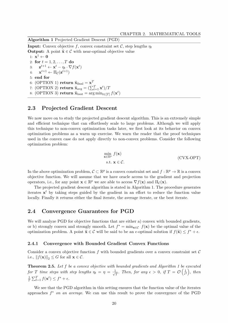
CHAPTER 2. MATHEMATICAL TOOLSAlgorithm 1 Projected Gradient Descent (PGD)Input: Convex objective f , convex constraint set C, step lengths ηtOutput: A point x ∈ C with near-optimal objective value1: x1 ← 02: for t = 1, 2, . . . , T do3: zt+1 ← xt − ηt · ∇f(xt)4: xt+1 ← ΠC(zt+1)5: end for6: (OPTION 1) return xfinal = xT7: (OPTION 2) return xavg = (
∑Tt=1 xt)/T
8: (OPTION 3) return xbest = arg mint∈[T ] f(xt)
2.3 Projected Gradient Descent
We now move on to study the projected gradient descent algorithm. This is an extremely simpleand efficient technique that can effortlessly scale to large problems. Although we will applythis technique to non-convex optimization tasks later, we first look at its behavior on convexoptimization problems as a warm up exercise. We warn the reader that the proof techniquesused in the convex case do not apply directly to non-convex problems. Consider the followingoptimization problem:
minx∈Rp
f(x)
s.t. x ∈ C.(CVX-OPT)
In the above optimization problem, C ⊂ Rp is a convex constraint set and f : Rp → R is a convexobjective function. We will assume that we have oracle access to the gradient and projectionoperators, i.e., for any point x ∈ Rp we are able to access ∇f(x) and ΠC(x).
The projected gradient descent algorithm is stated in Algorithm 1. The procedure generatesiterates xt by taking steps guided by the gradient in an effort to reduce the function valuelocally. Finally it returns either the final iterate, the average iterate, or the best iterate.
2.4 Convergence Guarantees for PGD
We will analyze PGD for objective functions that are either a) convex with bounded gradients,or b) strongly convex and strongly smooth. Let f∗ = minx∈C f(x) be the optimal value of theoptimization problem. A point x ∈ C will be said to be an ε-optimal solution if f(x) ≤ f∗ + ε.
2.4.1 Convergence with Bounded Gradient Convex Functions
Consider a convex objective function f with bounded gradients over a convex constraint set Ci.e., ‖f(x)‖2 ≤ G for all x ∈ C.
Theorem 2.5. Let f be a convex objective with bounded gradients and Algorithm 1 be executedfor T time steps with step lengths ηt = η = 1√
T. Then, for any ε > 0, if T = O
(1ε2
), then
1T
∑Tt=1 f(xt) ≤ f∗ + ε.
We see that the PGD algorithm in this setting ensures that the function value of the iteratesapproaches f∗ on an average. We can use this result to prove the convergence of the PGD
20

2.4. CONVERGENCE GUARANTEES FOR PGDalgorithm. If we use OPTION 3, i.e., xbest, then since by construction, we have f(xbest) ≤ f(xt)for all t, by applying Theorem 2.5, we get
f(xbest) ≤1T
T∑t=1
f(xt) ≤ f∗ + ε,
If we use OPTION 2, i.e., xavg, which is cheaper since we do not have to perform functionevaluations to find the best iterate, we can apply Jensen’s inequality (Lemma 2.1) to get thefollowing
f(xavg) = f
(1T
T∑t=1
xt)≤ 1T
T∑t=1
f(xt) ≤ f∗ + ε.
Note that the Jensen’s inequality may be applied only when the function f is convex. Now,whereas OPTION 1 i.e., xfinal, is the cheapest and does not require any additional operations,xfinal does not converge to the optimum for convex functions in general and may oscillate close tothe optimum. However, we shall shortly see that xfinal does converge if the objective function isstrongly smooth. Recall that strongly smooth functions may not grow at a faster-than-quadraticrate.
The reader would note that we have set the step length to a value that depends on thetotal number of iterations T for which the PGD algorithm is executed. This is called a horizon-aware setting of the step length. In case we are not sure what the value of T would be, ahorizon-oblivious setting of ηt = 1√
tcan also be shown to work4.
Proof (of Theorem 2.5). Let x∗ ∈ arg minx∈C f(x) denote any point in the constraint setwhere the optimum function value is achieved. Such a point always exists if the constraintset is closed and the objective function continuous. We will use the following potentialfunction Φt = f(xt) − f(x∗) to track the progress of the algorithm. Note that Φt measuresthe sub-optimality of the t-th iterate. Indeed, the statement of the theorem is equivalent toclaiming that 1
T
∑Tt=1 Φt ≤ ε.
(Apply Convexity) We apply convexity to upper bound the potential function at every step.Convexity is a global property and very useful in getting an upper bound on the level of sub-optimality of the current iterate in such analyses.
Φt = f(xt)− f(x∗) ≤⟨∇f(xt),xt − x∗
⟩We now do some elementary manipulations⟨
∇f(xt),xt − x∗⟩
= 1η
⟨η · ∇f(xt),xt − x∗
⟩= 1
2η
(∥∥∥xt − x∗∥∥∥2
2+∥∥∥η · ∇f(xt)
∥∥∥2
2−∥∥∥xt − η · ∇f(xt)− x∗
∥∥∥2
2
)= 1
2η
(∥∥∥xt − x∗∥∥∥2
2+∥∥∥η · ∇f(xt)
∥∥∥2
2−∥∥∥zt+1 − x∗
∥∥∥2
2
)≤ 1
2η
(∥∥∥xt − x∗∥∥∥2
2+ η2G2 −
∥∥∥zt+1 − x∗∥∥∥2
2
),
where the first step applies the identity 2ab = a2 +b2− (a+b)2, the second step uses the updatestep of the PGD algorithm that sets zt+1 ← xt − ηt · ∇f(xt), and the third step uses the factthat the objective function f has bounded gradients.
4See Exercise 2.4.
21
CHAPTER 2. MATHEMATICAL TOOLS(Apply Projection Property) We apply Lemma 2.4 to get∥∥∥zt+1 − x∗
∥∥∥2
2≥∥∥∥xt+1 − x∗
∥∥∥2
2
Putting all these together gives us
Φt ≤12η
(∥∥∥xt − x∗∥∥∥2
2−∥∥∥xt+1 − x∗
∥∥∥2
2
)+ ηG2
2
The above expression is interesting since it tells us that, apart from the ηG2/2 term which issmall as η = 1√
T, the current sub-optimality Φt is small if the consecutive iterates xt and xt+1
are close to each other (and hence similar in distance from x∗).This observation is quite useful since it tells us that once PGD stops making a lot of progress,
it actually converges to the optimum! In hindsight, this is to be expected. Since we are using aconstant step length, only a vanishing gradient can cause PGD to stop progressing. However,for convex functions, this only happens at global optima. Summing the expression up acrosstime steps, performing telescopic cancellations, using x1 = 0, and dividing throughout by Tgives us
1T
T∑t=1
Φt ≤1
2ηT(‖x∗‖22 − ‖x
T+1 − x∗‖22)
+ ηG2
2
≤ 12√T
(‖x∗‖22 +G2
),
where in the second step, we have used the fact that∥∥xt+1 − x∗
∥∥2 ≥ 0 and η = 1/
√T . This
gives us the claimed result.
2.4.2 Convergence with Strongly Convex and Smooth Functions
We will now prove a stronger guarantee for PGD when the objective function is strongly convexand strongly smooth (see Definition 2.4).
Theorem 2.6. Let f be an objective that satisfies the α-SC and β-SS properties. Let Algorithm 1be executed with step lengths ηt = η = 1
β . Then after at most T = O(βα log β
ε
)steps, we have
f(xT ) ≤ f(x∗) + ε.
This result is particularly nice since it ensures that the final iterate xfinal = xT converges,allowing us to use OPTION 1 in Algorithm 1 when the objective is SC/SS. A further advantageis the accelerated rate of convergence. Whereas for general convex functions, PGD requiresO(
1ε2
)iterations to reach an ε-optimal solution, for SC/SS functions, it requires only O
(log 1
ε
)iterations.
The reader would notice the insistence on the step length being set to η = 1β . In fact the
proof we show below crucially uses this setting. In practice, for many problems, β may not beknown to us or may be expensive to compute which presents a problem. However, as it turnsout, it is not necessary to set the step length exactly to 1/β. The result can be shown to holdeven for values of η < 1/β which are nevertheless large enough, but the proof becomes moreinvolved. In practice, the step length is tuned globally by doing a grid search over several ηvalues, or per-iteration using line search mechanisms, to obtain a step length value that assuresgood convergence rates.
22
2.4. CONVERGENCE GUARANTEES FOR PGDProof (of Theorem 2.6). This proof is a nice opportunity for the reader to see how the SC/SSproperties are utilized in a convergence analysis. As with convexity in the proof of Theorem 2.5,the strong convexity property is a global property that will be useful in assessing the progressmade so far by relating the optimal point x∗ with the current iterate xt. Strong smoothnesson the other hand, will be used locally to show that the procedure makes significant progressbetween iterates.
We will prove the result by showing that after at most T = O(βα log 1
ε
)steps, we will have∥∥∥xT − x∗
∥∥∥2
2≤ 2ε
β . This already tells us that we have reached very close to the optimum. However,we can use this to show that xT is ε-optimal in function value as well. Since we are very closeto the optimum, it makes sense to apply strong smoothness to upper bound the sub-optimalityas follows
f(xT ) ≤ f(x∗) +⟨∇f(x∗),xT − x∗
⟩+ β
2
∥∥∥xT − x∗∥∥∥2
2.
Now, since x∗ is an optimal point for the constrained optimization problem with a convexconstraint set C, the first order optimality condition [see Bubeck, 2015, Proposition 1.3] givesus 〈∇f(x∗),x− x∗〉 ≤ 0 for any x ∈ C. Applying this condition with x = xT gives us
f(xT )− f(x∗) ≤ β
2
∥∥∥xT − x∗∥∥∥2
2≤ ε,
which proves that xT is an ε-optimal point. We now show∥∥∥xT − x∗
∥∥∥2
2≤ 2ε
β . Given that wewish to show convergence in terms of the iterates, and not in terms of the function values, aswe did in Theorem 2.5, a natural potential function for this analysis is Φt =
∥∥xt − x∗∥∥2
2.
(Apply Strong Smoothness) As discussed before, we use it to show that PGD always makessignificant progress in each iteration.
f(xt+1)− f(xt) ≤⟨∇f(xt),xt+1 − xt
⟩+ β
2
∥∥∥xt − xt+1∥∥∥2
2
=⟨∇f(xt),xt+1 − x∗
⟩+⟨∇f(xt),x∗ − xt
⟩+ β
2
∥∥∥xt − xt+1∥∥∥2
2
= 1η
⟨xt − zt+1,xt+1 − xt
⟩+⟨∇f(xt),x∗ − xt
⟩+ β
2
∥∥∥xt − xt+1∥∥∥2
2
(Apply Projection Rule) The above expression contains an unwieldy term zt+1. Since thisterm only appears during projection steps, we eliminate it by applying Projection Property-I(Lemma 2.3) to get⟨
xt − zt+1,xt+1 − x∗⟩≤⟨xt − xt+1,xt+1 − x∗
⟩=∥∥xt − x∗
∥∥22 −
∥∥xt − xt+1∥∥22 −
∥∥xt+1 − x∗∥∥2
22
Using η = 1/β and combining the above results gives us
f(xt+1)− f(xt) ≤⟨∇f(xt),x∗ − xt
⟩+ β
2
(∥∥∥xt − x∗∥∥∥2
2−∥∥∥xt+1 − x∗
∥∥∥2
2
)(Apply Strong Convexity) The above expression is perfect for a telescoping step but for theinner product term. Fortunately, this can be eliminated using strong convexity.⟨
∇f(xt),x∗ − xt⟩≤ f(x∗)− f(xt)− α
2
∥∥∥xt − x∗∥∥∥2
2
23
CHAPTER 2. MATHEMATICAL TOOLSCombining with the above this gives us
f(xt+1)− f(x∗) ≤ β − α2
∥∥∥xt − x∗∥∥∥2
2− β
2
∥∥∥xt+1 − x∗∥∥∥2
2.
The above form seems almost ready for a telescoping exercise. However, something muchstronger can be said here, especially due to the −α2
∥∥xt − x∗∥∥2
2 term. Notice that we havef(xt+1) ≥ f(x∗). This means
β
2
∥∥∥xt+1 − x∗∥∥∥2
2≤ β − α
2
∥∥∥xt − x∗∥∥∥2
2,
which can be written asΦt+1 ≤
(1− α
β
)Φt ≤ exp
(−αβ
)Φt,
where we have used the fact that 1− x ≤ exp(−x) for all x ∈ R. What we have arrived at is avery powerful result as it assures us that the potential value goes down by a constant fractionat every iteration! Applying this result recursively gives us
Φt+1 ≤ exp(−αtβ
)Φ1 = exp
(−αtβ
)‖x∗‖22 ,
since x1 = 0. Thus, we deduce that ΦT =∥∥∥xT − x∗
∥∥∥2
2≤ 2ε
β after at most T = O(βα log β
ε
)steps
which finishes the proof
We notice that the convergence of the PGD algorithm is of the form∥∥xt+1 − x∗
∥∥22 ≤
exp(−αt
β
)‖x∗‖22. The number κ := β
α is the condition number of the optimization problem.The concept of condition number is central to numerical optimization. Below we give an infor-mal and generic definition for the concept. In later sections we will see the condition numberappearing repeatedly in the context of the convergence of various optimization algorithms forconvex, as well as non-convex problems. The exact numerical form of the condition number (forinstance here it is β/α) will also change depending on the application at hand. However, ingeneral, all these definitions of condition number will satisfy the following property.
Definition 2.6 (Condition Number - Informal). The condition number of a function f : X → Ris a scalar κ ∈ R that bounds how much the function value can change relative to a perturbationof the input.
Functions with a small condition number are stable and changes to their input do not affectthe function output values too much. However, functions with a large condition number canbe quite jumpy and experience abrupt changes in output values even if the input is changedslightly. To gain a deeper appreciation of this concept, consider a differentiable function f thatis also α-SC and β-SS. Consider a stationary point for f i.e., a point x such that ∇f(x) = 0.For a general function, such a point can be a local optima or a saddle point. However, since fis strongly convex, x is the (unique) global minima5 of f . Then we have, for any other point y
α
2 ‖x− y‖22 ≤ f(y)− f(x) ≤ β
2 ‖x− y‖22
Dividing throughout by α2 ‖x− y‖22 gives us
f(y)− f(x)α2 ‖x− y‖22
∈[1, βα
]:= [1, κ]
5See Exercise 2.5.
24

2.5. EXERCISESThus, upon perturbing the input from the global minimum x to a point ‖x− y‖2 =: ε distanceaway, the function value does change much – it goes up by an amount at least αε2
2 but at mostκ · αε22 . Such well behaved response to perturbations is very easy for optimization algorithms toexploit to give fast convergence.
The condition number of the objective function can significantly affect the convergence rateof algorithms. Indeed, if κ = β
α is small, then exp(−αβ
)= exp
(− 1κ
)would be small, ensuring
fast convergence. However, if κ 1 then exp(− 1κ
)≈ 1 and the procedure might offer slow
convergence.
2.5 ExercisesExercise 2.1. Show that strong smoothness does not imply convexity by constructing a non-convex function f : Rp → R that is 1-SS.
Exercise 2.2. Show that if a differentiable function f has bounded gradients i.e., ‖∇f(x)‖2 ≤ Gfor all x ∈ Rd, then f is Lipschitz. What is its Lipschitz constant?Hint: use the mean value theorem.
Exercise 2.3. Show that for any point z /∈ B2(r), the projection onto the ball is given byΠB2(r)(z) = r
‖z‖2· z.
Exercise 2.4. Show that a horizon-oblivious setting of ηt = 1√twhile executing the PGD algo-
rithm with a convex function with bounded gradients also ensures convergence.Hint: the convergence rates may be a bit different for this setting.
Exercise 2.5. Show that if f : Rp → R is a strongly convex function that is differentiable, thenthere is a unique point x∗ ∈ Rp that minimizes the function value f i.e., f(x∗) = minx∈Rp f(x).
Exercise 2.6. Show that the set of sparse vectors B0(s) ⊂ Rp is non-convex for any s < p.What happens when s = p?
Exercise 2.7. Show that Brank(r) ⊆ Rn×n, the set of n × n matrices with rank at most r, isnon-convex for any r < n. What happens when r = n?
Exercise 2.8. Consider the Cartesian product set C = Rm×r × Rn×r. Show that it is convex.
Exercise 2.9. Consider a least squares optimization problem with a strongly convex and smoothobjective. Show that the condition number of this problem is equal to the condition number ofthe Hessian matrix of the objective function.
Exercise 2.10. Show that if f : Rp → R is a strongly convex function that is differentiable,then optimization problems with f as an objective and a convex constraint set C always have aunique solution i.e., there is a unique point x∗ ∈ C that is a solution to the optimization problemarg minx∈C f(x). This generalizes the result in Exercise 2.5.Hint: use the first order optimality condition (see proof of Theorem 2.6)
2.6 Bibliographic NotesThe sole aim of this discussion was to give a self-contained introduction to concepts and tools inconvex analysis and descent algorithms in order to seamlessly introduce non-convex optimiza-tion techniques and their applications in subsequent sections. However, we clearly realize our
25

CHAPTER 2. MATHEMATICAL TOOLSinability to cover several useful and interesting results concerning convex functions and opti-mization techniques given the paucity of scope to present this discussion. We refer the reader toliterature in the field of optimization theory for a much more relaxed and deeper introductionto the area of convex optimization. Some excellent examples include [Bertsekas, 2016, Boyd andVandenberghe, 2004, Bubeck, 2015, Nesterov, 2003, Sra et al., 2011].
26

The official publication is available from now publishers viahttp://dx.doi.org/10.1561/2200000058
Part II
Non-convex Optimization Primitives
27
The official publication is available from now publishers viahttp://dx.doi.org/10.1561/2200000058
Chapter 3
Non-Convex Projected GradientDescent
In this section we will introduce and study gradient descent-style methods for non-convex op-timization problems. In § 2, we studied the projected gradient descent method for convex op-timization problems. Unfortunately, the algorithmic and analytic techniques used in convexproblems fail to extend to non-convex problems. In fact, non-convex problems are NP-hard tosolve and thus, no algorithmic technique should be expected to succeed on these problems ingeneral.
However, the situation is not so bleak. As we discussed in § 1, several breakthroughs in non-convex optimization have shown that non-convex problems that possess nice additional structurecan be solved not just in polynomial time, but rather efficiently too. Here, we will study the innerworkings of projected gradient methods on such structured non-convex optimization problems.
The discussion will be divided into three parts. The first part will take a look at constraintsets that, despite being non-convex, possess additional structure so that projections onto themcan be carried out efficiently. The second part will take a look at structural properties ofobjective functions that can aid optimization. The third part will present and analyze a simpleextension of the PGD algorithm for non-convex problems. We will see that for problems thatdo possess nicely structured objective functions and constraint sets, the PGD-style algorithmdoes converge to the global optimum in polynomial time with a linear rate of convergence.
We would like to point out to the reader that our emphasis in this section will be ongenerality and exposition of basic concepts. We will seek to present easily accessible analysesfor problems that have non-convex objectives. However, the price we will pay for this generalityis in the fineness of the results we present. The results discussed in this section are not the bestpossible and more refined and problem-specific results will be discussed in subsequent sectionswhere specific applications will be discussed in detail.
3.1 Non-Convex ProjectionsExecuting the projected gradient descent algorithm with non-convex problems requires projec-tions onto non-convex sets. Now, a quick look at the projection problem
ΠC(z) := arg minx∈C
‖x− z‖2
reveals that this is an optimization problem in itself. Thus, when the set C to be projected onto isnon-convex, the projection problem can itself be NP-hard. However, for several well-structuredsets, projection can be carried out efficiently despite the sets being non-convex.
28
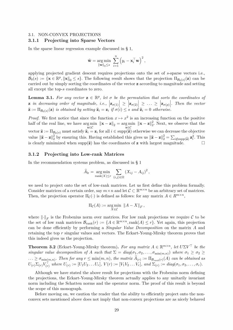
3.1. NON-CONVEX PROJECTIONS3.1.1 Projecting into Sparse Vectors
In the sparse linear regression example discussed in § 1,
w = arg min‖w‖0≤s
n∑i=1
(yi − x>i w
)2,
applying projected gradient descent requires projections onto the set of s-sparse vectors i.e.,B0(s) := x ∈ Rp, ‖x‖0 ≤ s. The following result shows that the projection ΠB0(s)(z) can becarried out by simply sorting the coordinates of the vector z according to magnitude and settingall except the top-s coordinates to zero.
Lemma 3.1. For any vector z ∈ Rp, let σ be the permutation that sorts the coordinates ofz in decreasing order of magnitude, i.e.,
∣∣∣zσ(1)
∣∣∣ ≥ ∣∣∣zσ(2)
∣∣∣ ≥ . . . ≥∣∣∣zσ(p)
∣∣∣. Then the vectorz := ΠB0(s)(z) is obtained by setting zi = zi if σ(i) ≤ s and zi = 0 otherwise.
Proof. We first notice that since the function x 7→ x2 is an increasing function on the positivehalf of the real line, we have arg min
x∈C‖x− z‖2 = arg min
x∈C‖x− z‖22. Next, we observe that the
vector z := ΠB0(s) must satisfy zi = zi for all i ∈ supp(z) otherwise we can decrease the objectivevalue ‖z− z‖22 by ensuring this. Having established this gives us ‖z− z‖22 =
∑i/∈supp(z) z2
i . Thisis clearly minimized when supp(z) has the coordinates of z with largest magnitude.
3.1.2 Projecting into Low-rank Matrices
In the recommendation systems problem, as discussed in § 1
Alr = arg minrank(X)≤r
∑(i,j)∈Ω
(Xij −Aij)2 ,
we need to project onto the set of low-rank matrices. Let us first define this problem formally.Consider matrices of a certain order, saym×n and let C ⊂ Rm×n be an arbitrary set of matrices.Then, the projection operator ΠC(·) is defined as follows: for any matrix A ∈ Rm×n,
ΠC(A) := arg minX∈C
‖A−X‖F ,
where ‖·‖F is the Frobenius norm over matrices. For low rank projections we require C to bethe set of low rank matrices Brank(r) := A ∈ Rm×n, rank(A) ≤ r. Yet again, this projectioncan be done efficiently by performing a Singular Value Decomposition on the matrix A andretaining the top r singular values and vectors. The Eckart-Young-Mirsky theorem proves thatthis indeed gives us the projection.
Theorem 3.2 (Eckart-Young-Mirsky theorem). For any matrix A ∈ Rm×n, let UΣV > be thesingular value decomposition of A such that Σ = diag(σ1, σ2, . . . , σmin(m,n)) where σ1 ≥ σ2 ≥. . . ≥ σmin(m,n). Then for any r ≤ min(m,n), the matrix A(r) := ΠBrank(r)(A) can be obtained asU(r)Σ(r)V
>(r) where U(r) := [U1U2 . . . Ur], V (r) := [V1V2 . . . Vr], and Σ(r) := diag(σ1, σ2, . . . , σr).
Although we have stated the above result for projections with the Frobenius norm definingthe projections, the Eckart-Young-Mirsky theorem actually applies to any unitarily invariantnorm including the Schatten norms and the operator norm. The proof of this result is beyondthe scope of this monograph.
Before moving on, we caution the reader that the ability to efficiently project onto the non-convex sets mentioned above does not imply that non-convex projections are as nicely behaved
29
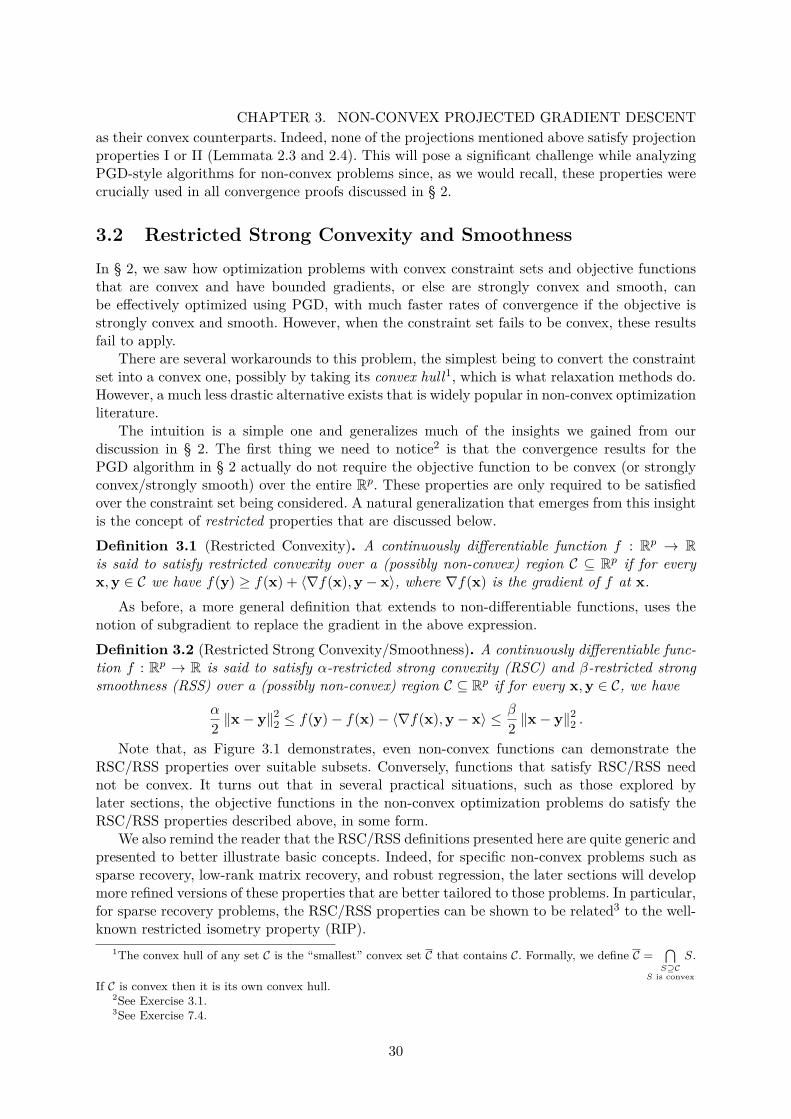
CHAPTER 3. NON-CONVEX PROJECTED GRADIENT DESCENTas their convex counterparts. Indeed, none of the projections mentioned above satisfy projectionproperties I or II (Lemmata 2.3 and 2.4). This will pose a significant challenge while analyzingPGD-style algorithms for non-convex problems since, as we would recall, these properties werecrucially used in all convergence proofs discussed in § 2.
3.2 Restricted Strong Convexity and SmoothnessIn § 2, we saw how optimization problems with convex constraint sets and objective functionsthat are convex and have bounded gradients, or else are strongly convex and smooth, canbe effectively optimized using PGD, with much faster rates of convergence if the objective isstrongly convex and smooth. However, when the constraint set fails to be convex, these resultsfail to apply.
There are several workarounds to this problem, the simplest being to convert the constraintset into a convex one, possibly by taking its convex hull1, which is what relaxation methods do.However, a much less drastic alternative exists that is widely popular in non-convex optimizationliterature.
The intuition is a simple one and generalizes much of the insights we gained from ourdiscussion in § 2. The first thing we need to notice2 is that the convergence results for thePGD algorithm in § 2 actually do not require the objective function to be convex (or stronglyconvex/strongly smooth) over the entire Rp. These properties are only required to be satisfiedover the constraint set being considered. A natural generalization that emerges from this insightis the concept of restricted properties that are discussed below.Definition 3.1 (Restricted Convexity). A continuously differentiable function f : Rp → Ris said to satisfy restricted convexity over a (possibly non-convex) region C ⊆ Rp if for everyx,y ∈ C we have f(y) ≥ f(x) + 〈∇f(x),y− x〉, where ∇f(x) is the gradient of f at x.
As before, a more general definition that extends to non-differentiable functions, uses thenotion of subgradient to replace the gradient in the above expression.Definition 3.2 (Restricted Strong Convexity/Smoothness). A continuously differentiable func-tion f : Rp → R is said to satisfy α-restricted strong convexity (RSC) and β-restricted strongsmoothness (RSS) over a (possibly non-convex) region C ⊆ Rp if for every x,y ∈ C, we have
α
2 ‖x− y‖22 ≤ f(y)− f(x)− 〈∇f(x),y− x〉 ≤ β
2 ‖x− y‖22 .
Note that, as Figure 3.1 demonstrates, even non-convex functions can demonstrate theRSC/RSS properties over suitable subsets. Conversely, functions that satisfy RSC/RSS neednot be convex. It turns out that in several practical situations, such as those explored bylater sections, the objective functions in the non-convex optimization problems do satisfy theRSC/RSS properties described above, in some form.
We also remind the reader that the RSC/RSS definitions presented here are quite generic andpresented to better illustrate basic concepts. Indeed, for specific non-convex problems such assparse recovery, low-rank matrix recovery, and robust regression, the later sections will developmore refined versions of these properties that are better tailored to those problems. In particular,for sparse recovery problems, the RSC/RSS properties can be shown to be related3 to the well-known restricted isometry property (RIP).
1The convex hull of any set C is the “smallest” convex set C that contains C. Formally, we define C =⋂S⊇C
S is convex
S.
If C is convex then it is its own convex hull.2See Exercise 3.1.3See Exercise 7.4.
30
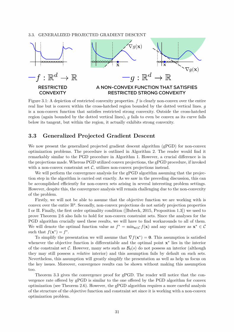
3.3. GENERALIZED PROJECTED GRADIENT DESCENT
RESTRICTED CONVEXITY
A NON-CONVEX FUNCTION THAT SATISFIES RESTRICTED STRONG CONVEXITY
Figure 3.1: A depiction of restricted convexity properties. f is clearly non-convex over the entirereal line but is convex within the cross-hatched region bounded by the dotted vertical lines. gis a non-convex function that satisfies restricted strong convexity. Outside the cross-hatchedregion (again bounded by the dotted vertical lines), g fails to even be convex as its curve fallsbelow its tangent, but within the region, it actually exhibits strong convexity.
3.3 Generalized Projected Gradient Descent
We now present the generalized projected gradient descent algorithm (gPGD) for non-convexoptimization problems. The procedure is outlined in Algorithm 2. The reader would find itremarkably similar to the PGD procedure in Algorithm 1. However, a crucial difference is inthe projections made. Whereas PGD utilized convex projections, the gPGD procedure, if invokedwith a non-convex constraint set C, utilizes non-convex projections instead.
We will perform the convergence analysis for the gPGD algorithm assuming that the projec-tion step in the algorithm is carried out exactly. As we saw in the preceding discussion, this canbe accomplished efficiently for non-convex sets arising in several interesting problem settings.However, despite this, the convergence analysis will remain challenging due to the non-convexityof the problem.
Firstly, we will not be able to assume that the objective function we are working with isconvex over the entire Rp. Secondly, non-convex projections do not satisfy projection propertiesI or II. Finally, the first order optimality condition ([Bubeck, 2015, Proposition 1.3]) we used toprove Theorem 2.6 also fails to hold for non-convex constraint sets. Since the analyses for thePGD algorithm crucially used these results, we will have to find workarounds to all of them.We will denote the optimal function value as f∗ = minx∈C f(x) and any optimizer as x∗ ∈ Csuch that f(x∗) = f∗.
To simplify the presentation we will assume that ∇f(x∗) = 0. This assumption is satisfiedwhenever the objective function is differentiable and the optimal point x∗ lies in the interiorof the constraint set C. However, many sets such as B0(s) do not possess an interior (althoughthey may still possess a relative interior) and this assumption fails by default on such sets.Nevertheless, this assumption will greatly simplify the presentation as well as help us focus onthe key issues. Moreover, convergence results can be shown without making this assumptiontoo.
Theorem 3.3 gives the convergence proof for gPGD. The reader will notice that the con-vergence rate offered by gPGD is similar to the one offered by the PGD algorithm for convexoptimization (see Theorem 2.6). However, the gPGD algorithm requires a more careful analysisof the structure of the objective function and constraint set since it is working with a non-convexoptimization problem.
31
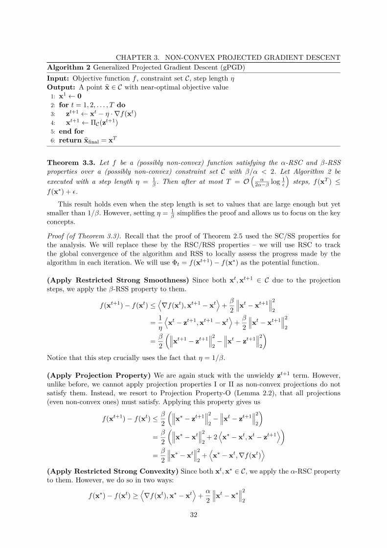
CHAPTER 3. NON-CONVEX PROJECTED GRADIENT DESCENTAlgorithm 2 Generalized Projected Gradient Descent (gPGD)Input: Objective function f , constraint set C, step length ηOutput: A point x ∈ C with near-optimal objective value1: x1 ← 02: for t = 1, 2, . . . , T do3: zt+1 ← xt − η · ∇f(xt)4: xt+1 ← ΠC(zt+1)5: end for6: return xfinal = xT
Theorem 3.3. Let f be a (possibly non-convex) function satisfying the α-RSC and β-RSSproperties over a (possibly non-convex) constraint set C with β/α < 2. Let Algorithm 2 beexecuted with a step length η = 1
β . Then after at most T = O(
α2α−β log 1
ε
)steps, f(xT ) ≤
f(x∗) + ε.
This result holds even when the step length is set to values that are large enough but yetsmaller than 1/β. However, setting η = 1
β simplifies the proof and allows us to focus on the keyconcepts.
Proof (of Theorem 3.3). Recall that the proof of Theorem 2.5 used the SC/SS properties forthe analysis. We will replace these by the RSC/RSS properties – we will use RSC to trackthe global convergence of the algorithm and RSS to locally assess the progress made by thealgorithm in each iteration. We will use Φt = f(xt+1)− f(x∗) as the potential function.
(Apply Restricted Strong Smoothness) Since both xt,xt+1 ∈ C due to the projectionsteps, we apply the β-RSS property to them.
f(xt+1)− f(xt) ≤⟨∇f(xt),xt+1 − xt
⟩+ β
2
∥∥∥xt − xt+1∥∥∥2
2
= 1η
⟨xt − zt+1,xt+1 − xt
⟩+ β
2
∥∥∥xt − xt+1∥∥∥2
2
= β
2
(∥∥∥xt+1 − zt+1∥∥∥2
2−∥∥∥xt − zt+1
∥∥∥2
2
)Notice that this step crucially uses the fact that η = 1/β.
(Apply Projection Property) We are again stuck with the unwieldy zt+1 term. However,unlike before, we cannot apply projection properties I or II as non-convex projections do notsatisfy them. Instead, we resort to Projection Property-O (Lemma 2.2), that all projections(even non-convex ones) must satisfy. Applying this property gives us
f(xt+1)− f(xt) ≤ β
2
(∥∥∥x∗ − zt+1∥∥∥2
2−∥∥∥xt − zt+1
∥∥∥2
2
)= β
2
(∥∥∥x∗ − xt∥∥∥2
2+ 2
⟨x∗ − xt,xt − zt+1
⟩)= β
2
∥∥∥x∗ − xt∥∥∥2
2+⟨x∗ − xt,∇f(xt)
⟩(Apply Restricted Strong Convexity) Since both xt,x∗ ∈ C, we apply the α-RSC propertyto them. However, we do so in two ways:
f(x∗)− f(xt) ≥⟨∇f(xt),x∗ − xt
⟩+ α
2
∥∥∥xt − x∗∥∥∥2
2
32
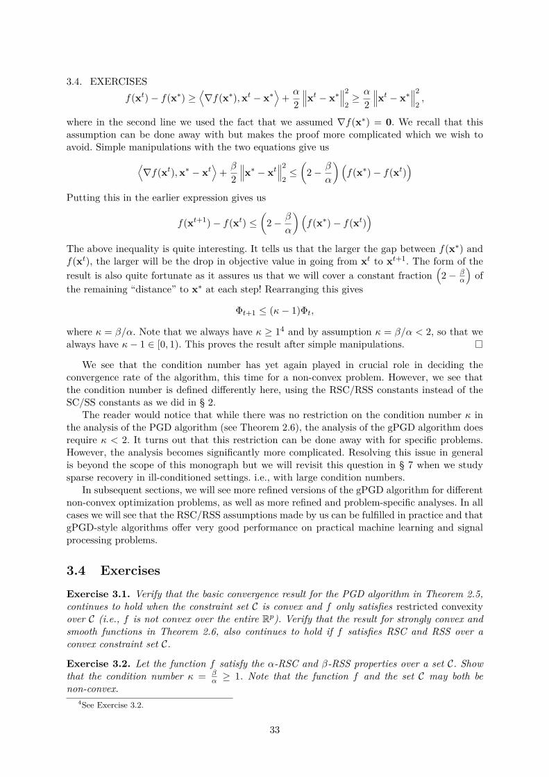
3.4. EXERCISESf(xt)− f(x∗) ≥
⟨∇f(x∗),xt − x∗
⟩+ α
2
∥∥∥xt − x∗∥∥∥2
2≥ α
2
∥∥∥xt − x∗∥∥∥2
2,
where in the second line we used the fact that we assumed ∇f(x∗) = 0. We recall that thisassumption can be done away with but makes the proof more complicated which we wish toavoid. Simple manipulations with the two equations give us⟨
∇f(xt),x∗ − xt⟩
+ β
2
∥∥∥x∗ − xt∥∥∥2
2≤(
2− β
α
)(f(x∗)− f(xt)
)Putting this in the earlier expression gives us
f(xt+1)− f(xt) ≤(
2− β
α
)(f(x∗)− f(xt)
)The above inequality is quite interesting. It tells us that the larger the gap between f(x∗) andf(xt), the larger will be the drop in objective value in going from xt to xt+1. The form of theresult is also quite fortunate as it assures us that we will cover a constant fraction
(2− β
α
)of
the remaining “distance” to x∗ at each step! Rearranging this gives
Φt+1 ≤ (κ− 1)Φt,
where κ = β/α. Note that we always have κ ≥ 14 and by assumption κ = β/α < 2, so that wealways have κ− 1 ∈ [0, 1). This proves the result after simple manipulations.
We see that the condition number has yet again played in crucial role in deciding theconvergence rate of the algorithm, this time for a non-convex problem. However, we see thatthe condition number is defined differently here, using the RSC/RSS constants instead of theSC/SS constants as we did in § 2.
The reader would notice that while there was no restriction on the condition number κ inthe analysis of the PGD algorithm (see Theorem 2.6), the analysis of the gPGD algorithm doesrequire κ < 2. It turns out that this restriction can be done away with for specific problems.However, the analysis becomes significantly more complicated. Resolving this issue in generalis beyond the scope of this monograph but we will revisit this question in § 7 when we studysparse recovery in ill-conditioned settings. i.e., with large condition numbers.
In subsequent sections, we will see more refined versions of the gPGD algorithm for differentnon-convex optimization problems, as well as more refined and problem-specific analyses. In allcases we will see that the RSC/RSS assumptions made by us can be fulfilled in practice and thatgPGD-style algorithms offer very good performance on practical machine learning and signalprocessing problems.
3.4 ExercisesExercise 3.1. Verify that the basic convergence result for the PGD algorithm in Theorem 2.5,continues to hold when the constraint set C is convex and f only satisfies restricted convexityover C (i.e., f is not convex over the entire Rp). Verify that the result for strongly convex andsmooth functions in Theorem 2.6, also continues to hold if f satisfies RSC and RSS over aconvex constraint set C.
Exercise 3.2. Let the function f satisfy the α-RSC and β-RSS properties over a set C. Showthat the condition number κ = β
α ≥ 1. Note that the function f and the set C may both benon-convex.
4See Exercise 3.2.
33

CHAPTER 3. NON-CONVEX PROJECTED GRADIENT DESCENTExercise 3.3. Recall the recommendation systems problem we discussed in § 1. Show thatassuming the ratings matrix to be rank-r is equivalent to assuming that with every user i ∈ [m]there is associated a vector ui ∈ Rr describing that user, and with every item j ∈ [n] there isassociated a vector vi ∈ Rr describing that item such that the rating given by user i to item jis Aij = u>i vj.Hint: Use the singular value decomposition for A.
34
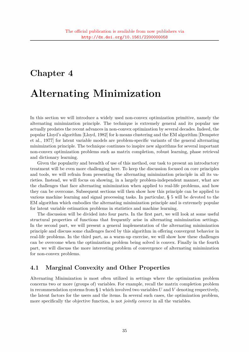
The official publication is available from now publishers viahttp://dx.doi.org/10.1561/2200000058
Chapter 4
Alternating Minimization
In this section we will introduce a widely used non-convex optimization primitive, namely thealternating minimization principle. The technique is extremely general and its popular useactually predates the recent advances in non-convex optimization by several decades. Indeed, thepopular Lloyd’s algorithm [Lloyd, 1982] for k-means clustering and the EM algorithm [Dempsteret al., 1977] for latent variable models are problem-specific variants of the general alternatingminimization principle. The technique continues to inspire new algorithms for several importantnon-convex optimization problems such as matrix completion, robust learning, phase retrievaland dictionary learning.
Given the popularity and breadth of use of this method, our task to present an introductorytreatment will be even more challenging here. To keep the discussion focused on core principlesand tools, we will refrain from presenting the alternating minimization principle in all its va-rieties. Instead, we will focus on showing, in a largely problem-independent manner, what arethe challenges that face alternating minimization when applied to real-life problems, and howthey can be overcome. Subsequent sections will then show how this principle can be applied tovarious machine learning and signal processing tasks. In particular, § 5 will be devoted to theEM algorithm which embodies the alternating minimization principle and is extremely popularfor latent variable estimation problems in statistics and machine learning.
The discussion will be divided into four parts. In the first part, we will look at some usefulstructural properties of functions that frequently arise in alternating minimization settings.In the second part, we will present a general implementation of the alternating minimizationprinciple and discuss some challenges faced by this algorithm in offering convergent behavior inreal-life problems. In the third part, as a warm-up exercise, we will show how these challengescan be overcome when the optimization problem being solved is convex. Finally in the fourthpart, we will discuss the more interesting problem of convergence of alternating minimizationfor non-convex problems.
4.1 Marginal Convexity and Other PropertiesAlternating Minimization is most often utilized in settings where the optimization problemconcerns two or more (groups of) variables. For example, recall the matrix completion problemin recommendation systems from § 1 which involved two variables U and V denoting respectively,the latent factors for the users and the items. In several such cases, the optimization problem,more specifically the objective function, is not jointly convex in all the variables.
35
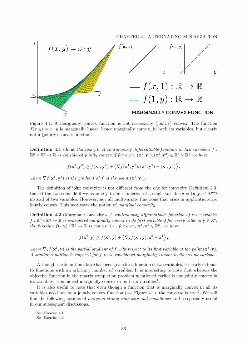
CHAPTER 4. ALTERNATING MINIMIZATION
MARGINALLY CONVEX FUNCTION
Figure 4.1: A marginally convex function is not necessarily (jointly) convex. The functionf(x, y) = x · y is marginally linear, hence marginally convex, in both its variables, but clearlynot a (jointly) convex function.
Definition 4.1 (Joint Convexity). A continuously differentiable function in two variables f :Rp × Rq → R is considered jointly convex if for every (x1,y1), (x2,y2) ∈ Rp × Rq we have
f(x2,y2) ≥ f(x1,y1) +⟨∇f(x1,y1), (x2,y2)− (x1,y1)
⟩,
where ∇f(x1,y1) is the gradient of f at the point (x1,y1).
The definition of joint convexity is not different from the one for convexity Definition 2.3.Indeed the two coincide if we assume f to be a function of a single variable z = (x,y) ∈ Rp+qinstead of two variables. However, not all multivariate functions that arise in applications arejointly convex. This motivates the notion of marginal convexity.
Definition 4.2 (Marginal Convexity). A continuously differentiable function of two variablesf : Rp×Rq → R is considered marginally convex in its first variable if for every value of y ∈ Rq,the function f(·,y) : Rp → R is convex, i.e., for every x1,x2 ∈ Rp, we have
f(x2,y) ≥ f(x1,y) +⟨∇xf(x1,y),x2 − x1
⟩,
where ∇xf(x1,y) is the partial gradient of f with respect to its first variable at the point (x1,y).A similar condition is imposed for f to be considered marginally convex in its second variable.
Although the definition above has been given for a function of two variables, it clearly extendsto functions with an arbitrary number of variables. It is interesting to note that whereas theobjective function in the matrix completion problem mentioned earlier is not jointly convex inits variables, it is indeed marginally convex in both its variables1.
It is also useful to note that even though a function that is marginally convex in all itsvariables need not be a jointly convex function (see Figure 4.1), the converse is true2. We willfind the following notions of marginal strong convexity and smoothness to be especially usefulin our subsequent discussions.
1See Exercise 4.1.2See Exercise 4.2.
36
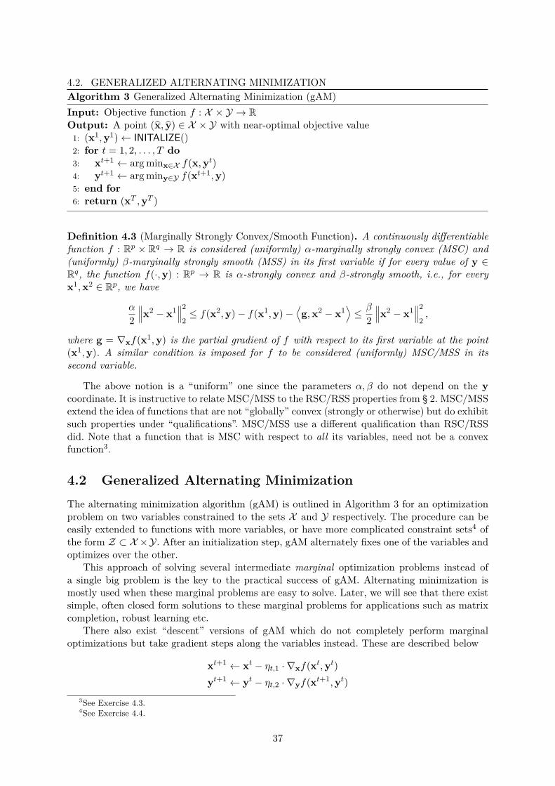
4.2. GENERALIZED ALTERNATING MINIMIZATIONAlgorithm 3 Generalized Alternating Minimization (gAM)Input: Objective function f : X × Y → ROutput: A point (x, y) ∈ X × Y with near-optimal objective value1: (x1,y1)← INITALIZE()2: for t = 1, 2, . . . , T do3: xt+1 ← arg minx∈X f(x,yt)4: yt+1 ← arg miny∈Y f(xt+1,y)5: end for6: return (xT ,yT )
Definition 4.3 (Marginally Strongly Convex/Smooth Function). A continuously differentiablefunction f : Rp × Rq → R is considered (uniformly) α-marginally strongly convex (MSC) and(uniformly) β-marginally strongly smooth (MSS) in its first variable if for every value of y ∈Rq, the function f(·,y) : Rp → R is α-strongly convex and β-strongly smooth, i.e., for everyx1,x2 ∈ Rp, we have
α
2
∥∥∥x2 − x1∥∥∥2
2≤ f(x2,y)− f(x1,y)−
⟨g,x2 − x1
⟩≤ β
2
∥∥∥x2 − x1∥∥∥2
2,
where g = ∇xf(x1,y) is the partial gradient of f with respect to its first variable at the point(x1,y). A similar condition is imposed for f to be considered (uniformly) MSC/MSS in itssecond variable.
The above notion is a “uniform” one since the parameters α, β do not depend on the ycoordinate. It is instructive to relate MSC/MSS to the RSC/RSS properties from § 2. MSC/MSSextend the idea of functions that are not “globally” convex (strongly or otherwise) but do exhibitsuch properties under “qualifications”. MSC/MSS use a different qualification than RSC/RSSdid. Note that a function that is MSC with respect to all its variables, need not be a convexfunction3.
4.2 Generalized Alternating MinimizationThe alternating minimization algorithm (gAM) is outlined in Algorithm 3 for an optimizationproblem on two variables constrained to the sets X and Y respectively. The procedure can beeasily extended to functions with more variables, or have more complicated constraint sets4 ofthe form Z ⊂ X ×Y. After an initialization step, gAM alternately fixes one of the variables andoptimizes over the other.
This approach of solving several intermediate marginal optimization problems instead ofa single big problem is the key to the practical success of gAM. Alternating minimization ismostly used when these marginal problems are easy to solve. Later, we will see that there existsimple, often closed form solutions to these marginal problems for applications such as matrixcompletion, robust learning etc.
There also exist “descent” versions of gAM which do not completely perform marginaloptimizations but take gradient steps along the variables instead. These are described below
xt+1 ← xt − ηt,1 · ∇xf(xt,yt)yt+1 ← yt − ηt,2 · ∇yf(xt+1,yt)
3See Exercise 4.3.4See Exercise 4.4.
37
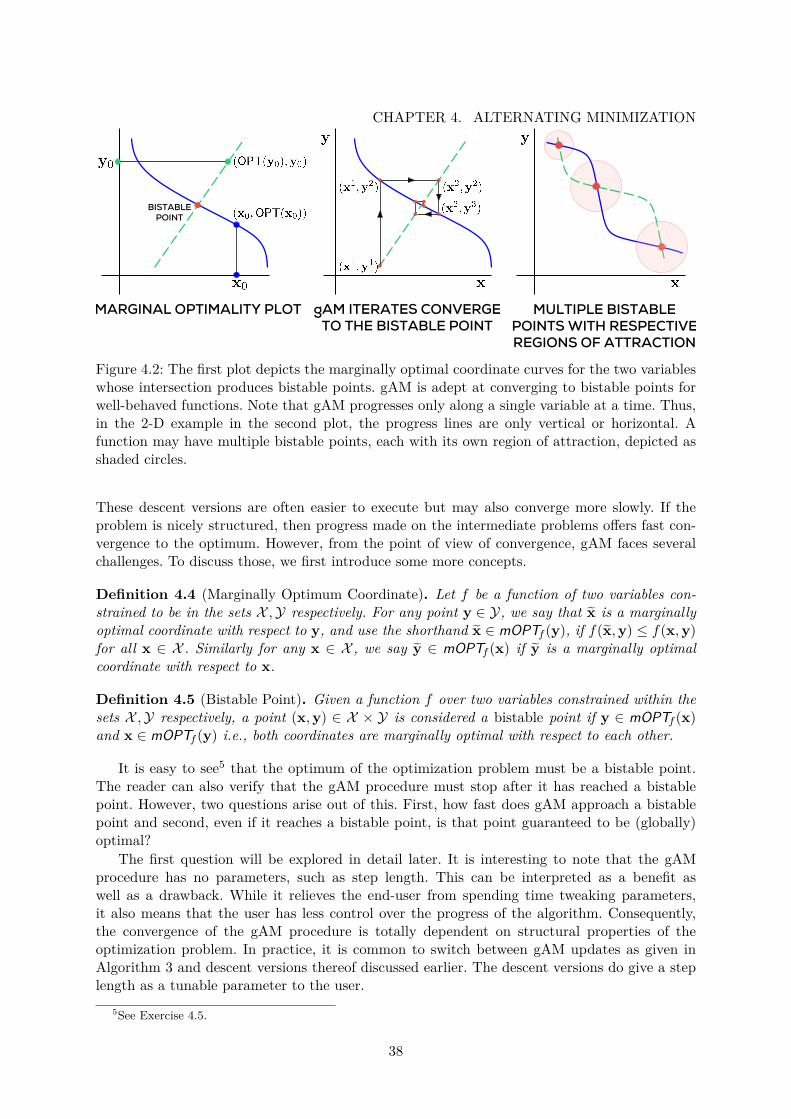
CHAPTER 4. ALTERNATING MINIMIZATION
MARGINAL OPTIMALITY PLOT
BISTABLE POINT
gAM ITERATES CONVERGE TO THE BISTABLE POINT
MULTIPLE BISTABLE POINTS WITH RESPECTIVE REGIONS OF ATTRACTION
Figure 4.2: The first plot depicts the marginally optimal coordinate curves for the two variableswhose intersection produces bistable points. gAM is adept at converging to bistable points forwell-behaved functions. Note that gAM progresses only along a single variable at a time. Thus,in the 2-D example in the second plot, the progress lines are only vertical or horizontal. Afunction may have multiple bistable points, each with its own region of attraction, depicted asshaded circles.
These descent versions are often easier to execute but may also converge more slowly. If theproblem is nicely structured, then progress made on the intermediate problems offers fast con-vergence to the optimum. However, from the point of view of convergence, gAM faces severalchallenges. To discuss those, we first introduce some more concepts.
Definition 4.4 (Marginally Optimum Coordinate). Let f be a function of two variables con-strained to be in the sets X ,Y respectively. For any point y ∈ Y, we say that x is a marginallyoptimal coordinate with respect to y, and use the shorthand x ∈ mOPTf (y), if f(x,y) ≤ f(x,y)for all x ∈ X . Similarly for any x ∈ X , we say y ∈ mOPTf (x) if y is a marginally optimalcoordinate with respect to x.
Definition 4.5 (Bistable Point). Given a function f over two variables constrained within thesets X ,Y respectively, a point (x,y) ∈ X × Y is considered a bistable point if y ∈ mOPTf (x)and x ∈ mOPTf (y) i.e., both coordinates are marginally optimal with respect to each other.
It is easy to see5 that the optimum of the optimization problem must be a bistable point.The reader can also verify that the gAM procedure must stop after it has reached a bistablepoint. However, two questions arise out of this. First, how fast does gAM approach a bistablepoint and second, even if it reaches a bistable point, is that point guaranteed to be (globally)optimal?
The first question will be explored in detail later. It is interesting to note that the gAMprocedure has no parameters, such as step length. This can be interpreted as a benefit aswell as a drawback. While it relieves the end-user from spending time tweaking parameters,it also means that the user has less control over the progress of the algorithm. Consequently,the convergence of the gAM procedure is totally dependent on structural properties of theoptimization problem. In practice, it is common to switch between gAM updates as given inAlgorithm 3 and descent versions thereof discussed earlier. The descent versions do give a steplength as a tunable parameter to the user.
5See Exercise 4.5.
38
4.3. A CONVERGENCE GUARANTEE FOR GAM FOR CONVEX PROBLEMSThe second question requires a closer look at the interaction between the objective function
and the gAM process. Figure 4.2 illustrates this with toy bi-variate functions over R2. In thefirst figure, the bold solid curve plots the function g : X → X × Y with g(x) = (x,mOPTf (x))(in this toy case, the marginally optimal coordinates are taken to be unique for simplicity, i.e.,|mOPTf (x)| = 1 for all x ∈ X ). The bold dashed curve similarly plots h : Y → X × Y withh(y) = (mOPTf (y),y). These plots are quite handy in demonstrating the convergence propertiesof the gAM algorithm.
It is easy to see that bistable points lie precisely at the intersection of the bold solid andthe bold dashed curves. The second illustration shows how the gAM process may behave wheninstantiated with this toy function – clearly gAM exhibits rapid convergence to the bistablepoint. However, the third illustration shows that functions may have multiple bistable points.The figure shows that this may happen even if the marginally optimal coordinates are uniquei.e., for every x there is a unique y such that y = mOPTf (x) and vice versa.
In case a function taking bounded values possesses multiple bistable points, the bistablepoint to which gAM eventually converges depends on where the procedure was initialized. This isexemplified in the third illustration where each bistable region has its own “region of attraction”.If initialized inside a particular region, gAM converges to the bistable point corresponding tothat region. This means that in order to converge to the globally optimal point, gAM must beinitialized inside the region of attraction of the global optimum.
The above discussion shows that it may be crucial to properly initialize the gAM procedureto ensure convergence to the global optimum. Indeed, when discussing gAM-style algorithms forlearning latent variable models, matrix completion and phase retrieval in later sections, we willpay special attention to initialize the procedure “close” to the optimum. The only exception willbe that of robust regression in § 9 where it seems that the problem structure ensures a uniquebistable point and so, a careful initialization is not required.
4.3 A Convergence Guarantee for gAM for Convex Problems
As usual, things do become nice when the optimization problems are convex. For instance, fordifferentiable convex functions, all bistable points are global minima6 and thus, converging toany one of them is sufficient. In fact, approaches similar to gAM, commonly known as Coordi-nate Minimization (CM), are extremely popular for large scale convex optimization problems.The CM procedure simply treats a single p-dimensional variable x ∈ Rp as p one-dimensionalvariables x1, . . . ,xp and executes gAM-like steps with them, resulting in the intermediateproblems being uni-dimensional. However, it is worth noting that gAM can struggle with non-differentiable objectives.
In the following, we will analyze the convergence of the gAM algorithm for the case whenthe objective function is jointly convex in both its variables. We will then see what happens toAlgorithm 3 if the function f is non-convex. To keep the discussion focused, we will consider anunconstrained optimization problem.
Theorem 4.1. Let f : Rp × Rq → R be jointly convex, continuously differentiable, sat-isfy β-MSS in both its variables, and f∗ = minx,y f(x,y) > −∞. Let the region S0 =x,y : f(x,y) ≤ f(0,0) ⊂ Rp+q be bounded, i.e., satisfy S0 ⊆ B2((0,0), R) for some R > 0. LetAlgorithm 3 be executed with the initialization (x1,y1) = (0,0). Then after at most T = O
(1ε
)steps, we have f(xT ,yT ) ≤ f∗ + ε.
6See Exercise 4.6.
39
CHAPTER 4. ALTERNATING MINIMIZATIONProof. The first property of the gAM algorithm that we need to appreciate is monotonicity. Itis easy to see that due to the marginal minimizations carried out, we have at all time steps t,
f(xt+1,yt+1) ≤ f(xt+1,yt) ≤ f(xt,yt)
The region S0 is the sublevel set of f at the initialization point. Due to the monotonicityproperty, we have f(xt,yt) ≤ f(x1,y1) for all t i.e., (xt,yt) ∈ S0 for all t. Thus, gAM remainsrestricted to the bounded region S0 and does not diverge. We notice that this point underliesthe importance of proper initialization: gAM benefits from being initialized at a point at whichthe sublevel set of f is bounded.
We will use Φt = 1f(xt,yt)−f∗ as the potential function. This is a slightly unusual choice of
potential function but its utility will be clear from the proof. Note that Φt > 0 for all t and thatconvergence is equivalent to showing Φt →∞. We will, as before, use smoothness to analyze theper-iteration progress made by gAM and use convexity for global convergence analysis. For anytime step t ≥ 2, consider the hypothetical update we could have made had we done a gradientstep instead of the marginal minimization step gAM does in step 3.
xt+1 = xt − 1β∇xf(xt,yt)
(Apply Marginal Strong Smoothness) We get
f(xt+1,yt) ≤ f(xt,yt) +⟨∇xf(xt,yt), xt+1 − xt,+
⟩ β2
∥∥∥xt+1 − xt∥∥∥2
2
= f(xt,yt)− 12β
∥∥∥∇xf(xt,yt)∥∥∥2
2
(Apply Monotonicity of gAM) Since xt+1 ∈ mOPTf (yt), we must have f(xt+1,yt) ≤f(xt+1,yt), which gives us
f(xt+1,yt+1) ≤ f(xt+1,yt) ≤ f(xt,yt)− 12β
∥∥∥∇xf(xt,yt)∥∥∥2
2
Now since t ≥ 2, we must have had yt ∈ arg miny f(xt,y). Since f is differentiable, we musthave ([see Bubeck, 2015, Proposition 1.2]) ∇yf(xt,yt) = 0. Applying the Pythagoras’ theoremnow gives us as a result,
∥∥∇f(xt,yt)∥∥2
2 =∥∥∇xf(xt,yt)
∥∥22.
(Apply Convexity) Since f is jointly convex, we can state
f(xt,yt)− f∗ ≤⟨∇f(xt,yt), (xt,yt)− (x∗,y∗)
⟩≤ 2R
∥∥∥∇f(xt,yt)∥∥∥
2,
where we have used the Cauchy-Schwartz inequality and the fact that (xt,yt), (x∗,y∗) ∈ S0.Putting these together gives us
f(xt+1,yt+1) ≤ f(xt,yt)− 14βR2
(f(xt,yt)− f∗
)2,
or in other words,1
Φt+1≤ 1
Φt− 1
4βR21
Φ2t
≤ 1Φt− 1
4βR21
ΦtΦt+1,
where the second step follows from monotonicity. Rearranging gives us
Φt+1 − Φt ≥1
4βR2 ,
40
4.4. A CONVERGENCE GUARANTEE FOR GAM UNDER MSC/MSSwhich upon telescoping, and using Φ2 ≥ 0 gives us
ΦT ≥T
4βR2 ,
which proves the result. Note that the result holds even if f is jointly convex and satisfies theMSS property only locally in the region S0.
4.4 A Convergence Guarantee for gAM under MSC/MSSWe will now investigate what happens when the gAM algorithm is executed with a non-convexfunction. Note that the previous result crucially uses convexity and will not extend here. More-over, for non-convex functions, there is no assurance that all bistable points are global minima.Instead we will have to fend for fast convergence to a bistable point, as well as show that thefunction is globally minimized there.
Doing the above will require additional structure on the objective function. In the following,we will denote f∗ = minx,y f(x,y) to be the optimum value of the objective function. We willfix (x∗,y∗) to be any point such that f(x∗,y∗) = f∗ (there may be several). We will also letZ∗ ⊂ Rp × Rq denote the set of all bistable points for f .
First of all, notice that if a continuously differentiable function f : Rp×Rq → R is marginallyconvex (strongly or otherwise) in both its variables, then its bistable points are exactly itsstationary points.
Lemma 4.2. A point (x,y) is bistable with respect to a continuously differentiable functionf : Rp × Rq that is marginally convex in both its variables iff ∇f(x,y) = 0.
Proof. It is easy to see that partial derivatives must vanish at a bistable point since thefunction is differentiable ([see Bubeck, 2015, Proposition 1.2]) and thus we get ∇f(x,y) =[∇xf(x,y),∇yf(x,y)] = 0. Arguing the other way round, if the gradient, and by extension thepartial derivatives, vanish at (x,y), then by marginal convexity, for any x′
f(x′,y)− f(x,y) ≥⟨∇xf(x,y),x′ − x
⟩= 0
Similarly, f(x,y′) ≥ f(x,y) for any y′. Thus (x,y) is bistable.
The above tells us that Z∗ is also the set of all stationary points of f . However, not allpoints in Z∗ may be global minima. Addressing this problem requires careful initialization andproblem-specific analysis, that we will carry out for problems such as matrix completion etc inlater sections. For now, we introduce a generic robust bistability property that will be very usefulin the analysis. Similar properties are frequently used in the analysis of gAM-style algorithms.
Definition 4.6 (Robust Bistability Property). A function f : Rp × Rq → R satisfies the C-robust bistability property if for some C > 0, for every (x,y) ∈ Rp × Rq, y ∈ mOPTf (x) andx ∈ mOPTf (y), we have
f(x,y∗) + f(x∗,y)− 2f∗ ≤ C · (2f(x,y)− f(x, y)− f(x,y)) .
The right hand expression captures how much one can reduce the function value locally byperforming marginal optimizations. The property suggests7 that if not much local improvementcan be made (i.e., if f(x, y) ≈ f(x,y) ≈ f(x,y)) then we are close to the optimum. This has asimple corollary that all bistable points achieve the (globally) optimal function value. We nowpresent a convergence analysis for gAM.
7See Exercise 4.7.
41
CHAPTER 4. ALTERNATING MINIMIZATIONTheorem 4.3. Let f : Rp × Rq → R be a continuously differentiable (but possibly non-convex)function that, within the region S0 = x,y : f(x,y) ≤ f(0,0) ⊂ Rp+q, satisfies the propertiesof α-MSC, β-MSS in both its variables, and C-robust bistability. Let Algorithm 3 be executedwith the initialization (x1,y1) = (0,0). Then after at most T = O
(log 1
ε
)steps, we have
f(xT ,yT ) ≤ f∗ + ε.
Note that the MSC/MSS and robust bistability properties need only hold within the sublevelset S0. This again underlines the importance of proper initialization. Also note that gAM offersrapid convergence despite the non-convexity of the objective. In order to prove the result, thefollowing consequence of C-robust bistability will be useful.
Lemma 4.4. Let f satisfy the properties mentioned in Theorem 4.3. Then for any (x,y) ∈Rp × Rq, y ∈ mOPTf (x) and x ∈ mOPTf (y),
‖x− x∗‖22 + ‖y− y∗‖22 ≤Cβ
α
(‖x− x‖22 + ‖y− y‖22
)Proof. Applying MSC/MSS repeatedly gives us
f(x,y∗) + f(x∗,y) ≥ 2f∗ + α
2(‖x− x∗‖22 + ‖y− y∗‖22
)2f(x,y) ≤ f(x, y) + f(x,y) + β
2(‖x− x‖22 + ‖y− y‖22
)Applying robust stability then proves the result.
It is noteworthy that Lemma 4.4 relates local convergence to global convergence and assuresus that reaching an almost bistable point is akin to converging to the optimum. Such a resultcan be crucial, especially for non-convex problems. Indeed, similar properties are used in otherproofs concerning coordinate minimization as well, for example, the local error bound used in[Luo and Tseng, 1993].
Proof (of Theorem 4.3). We will use Φt = f(xt,yt) − f∗ as the potential function. Since theintermediate steps in gAM are marginal optimizations and not gradient steps, we will actuallyfind it useful to apply marginal strong convexity at a local level, and apply marginal strongsmoothness at a global level instead.
(Apply Marginal Strong Smoothness) As ∇xf(x∗,y∗) = 0, applying MSS gives us
f(xt+1,y∗)− f(x∗,y∗) ≤ β
2
∥∥∥xt+1 − x∗∥∥∥2
2.
Further, the gAM updates ensure yt+1 ∈ mOPTf (xt+1), which gives
Φt+1 = f(xt+1,yt+1)− f∗ ≤ f(xt+1,y∗)− f∗ ≤ β
2
∥∥∥xt+1 − x∗∥∥∥2
2,
(Apply Marginal Strong Convexity) Since ∇xf(xt+1,yt) = 0,
f(xt,yt) ≥ f(xt+1,yt) + α
2
∥∥∥xt+1 − xt∥∥∥2
2
≥ f(xt+1,yt+1) + α
2
∥∥∥xt+1 − xt∥∥∥2
2,
which gives usΦt − Φt+1 ≥
α
2
∥∥∥xt+1 − xt∥∥∥2
2.
42
4.5. EXERCISESThis shows that appreciable progress is made in a single step. Now, with (xt,yt) for any t ≥ 2,due to the nature of the gAM updates, we know that yt ∈ mOPTf (xt) and xt+1 ∈ mOPTf (yt).Applying Lemma 4.4 then gives us the following inequality∥∥∥xt − x∗
∥∥∥2
2≤∥∥∥xt − x∗
∥∥∥2
2+∥∥∥yt − y∗
∥∥∥2
2≤ Cβ
α
∥∥∥xt − xt+1∥∥∥2
2
Putting these together and using (a+ b)2 ≤ 2(a2 + b2) gives us
Φt+1 ≤β
2
∥∥∥xt+1 − x∗∥∥∥2
2≤ β
(∥∥∥xt+1 − xt∥∥∥2
2+∥∥∥xt − x∗
∥∥∥2
2
)≤ β(1 + Cκ)
∥∥∥xt+1 − xt∥∥∥2
2≤ 2κ(1 + Cκ) (Φt − Φt+1) ,
where κ = βα is the effective condition number of the problem. Rearranging gives us
Φt+1 ≤ η0 · Φt,
where η0 = 2κ(1+Cκ)1+2κ(1+Cκ) < 1 which proves the result.
Notice that the condition number κ makes an appearance in the convergence rate of thealgorithm but this time, with a fresh definition in terms of the MSC/MSS parameters. Asbefore, small values of κ and C ensure fast convergence, whereas large values of κ,C promoteη0 → 1 which slows the procedure down.
Before we conclude, we remind the reader that in later sections, we will see more preciseanalyses of gAM-style approaches, and the structural assumptions will be more problem specific.However, we hope the preceding discussion has provided some insight into the inner workingsof alternating minimization techniques.
4.5 ExercisesExercise 4.1. Recall the low-rank matrix completion problem in recommendation systems from§ 1
Alv = minU∈Rm×rV ∈Rn×r
∑(i,j)∈Ω
(U>i Vj −Aij
)2.
Show that the objective in this optimization problem is not jointly convex in U and V . Thenshow that the objective is nevertheless, marginally convex in both the variables.
Exercise 4.2. Show that a function that is jointly convex is necessarily marginally convex aswell. Similarly show that a (jointly) strongly convex and smooth function is marginally so aswell.
Exercise 4.3. Marginal strong convexity does not imply convexity. Show this by giving anexample of a function f : Rp ×Rq → R that is marginally strongly convex in both its variables,but non-convex.Hint: use the fact that the function f(x) = x2 is 2-strongly convex.
Exercise 4.4. Design a variant of the gAM procedure that can handle a general constraint setZ ⊂ X × Y. Attempt to analyze the convergence of your algorithm.
Exercise 4.5. Show that (x∗,y∗) ∈ arg minx∈X ,y∈Y f(x,y) must be a bistable point for anyfunction even if f is non-convex.
43
CHAPTER 4. ALTERNATING MINIMIZATIONExercise 4.6. Let f : Rp × Rq → R be a differentiable, jointly convex function. Show that anybistable point of f is a global minimum for f .Hint: first show that directional derivatives vanish at bistable points.
Exercise 4.7. For a robustly bistable function f , any almost bistable point is almost opti-mal as well. Show this by proving, for any (x,y), y ∈ mOPTf (x), x ∈ mOPTf (y) such thatmax f(x, y), f(x,y) ≤ f(x,y) + ε, that f(x,y) ≤ f∗ + O (ε). Conclude that if f satisfiesrobust bistability, then any bistable point (x,y) ∈ Z∗ is optimal.
Exercise 4.8. Show that marginal strong convexity is additive i.e., if f, g : Rp × Rq → R aretwo functions such that f is respectively α1 and α2-MSC in its two variables and g is α1 andα2-MSC in its variables, then the function f+g is (α1 +α1) and (α2 +α2)-MSC in its variables.
Exercise 4.9. The alternating minimization procedure may oscillate if the optimization problemis not well-behaved. Suppose for an especially nasty problem, the gAM procedure enters into thefollowing loop
(xt,yt)→ (xt+1,yt)→ (xt+1,yt+1)→ (xt,yt+1)→ (xt,yt)
Show that all four points in the loop are bistable and share the same function value. Can youdraw a hypothetical set of marginally optimal coordinate curves which may cause this to happen(see Figure 4.2)?
4.6 Bibliographic NotesThe descent version for CM is aptly named Coordinate Descent (CD) and only takes descentsteps along the coordinates [Saha and Tewari, 2013]. There exist versions of CM and CD forconstrained optimization problems as well [Luo and Tseng, 1993, Nesterov, 2012]. A variant ofCM/CD splits variables into blocks of multi-dimensional variables. The resulting algorithm isappropriately named Block Coordinate Descent and minimizes over one block of variables ateach time step.
The coordinate/block being processed at each step is chosen carefully to ensure rapid con-vergence. Several “rules” exist for this, for example, the Gauss-Southwell rule (that chooses thecoordinate/block along which the objective gradient is the largest), the cyclic rule that sim-ply performs a round-robin selection of coordinates/blocks, and random choice that chooses arandom coordinate/block at each time step, independent of previous such choices.
For several problem areas such support vector machines, CM/CD methods are at the heartof some of the fastest solvers available due to their speed and ease of implementation [Fan et al.,2008, Luo and Tseng, 1992, Shalev-Shwartz and Zhang, 2013].
44
The official publication is available from now publishers viahttp://dx.doi.org/10.1561/2200000058
Chapter 5
The EM Algorithm
In this section we will take a look at the Expectation Maximization (EM) principle. The principleforms the basis for widely used learning algorithms such as those used for learning Gaussianmixture models, the Baum-Welch algorithm for learning hidden Markov models (HMM), andmixed regression. The EM algorithm is also a close cousin to the Lloyd’s algorithm for clusteringwith the k-means objective.
Although the EM algorithm, at a surface level, follows the alternating minimizationprinciple which we studied in § 5, given its wide applicability in learning latent variable modelsin probabilistic learning settings, we feel it is instructive to invest in a deeper understanding ofthe EM method. To make the reading experience self-contained, we will first devote some timedeveloping intuitions and notation in probabilistic learning methods.
Notation A parametric distribution over a domain X with parameter θ is denoted by f(· |θ)or fθ. The notation is abused to let f(x |θ) denote the probability mass or density function(as the case may be) of the distribution at the point x ∈ X . The notation is also abused to letX ∼ f(· |θ) or X ∼ fθ denote a sample drawn from this distribution.
5.1 A Primer in Probabilistic Machine Learning
Suppose we observe i.i.d. samples x1,x2, . . . ,xn of a random variable X ∈ X drawn froman unknown distribution f∗. Suppose also, that it is known that the distribution generatingthese data samples belongs to a parametric family of distributions F = fθ : θ ∈ Θ such thatf∗ = fθ∗ for some unknown parameter θ∗ ∈ Θ.
How may we recover (an accurate estimate of) the true parameter θ∗, using only the samplesx1, . . . ,xn? There are several ways to do so, popular among them being the maximum likelihoodestimate. Since the samples were generated independently, one can, for any parameter θ0 ∈ Θ,write their joint density function as follows
f(x1,x2, . . . ,xn |θ0) =n∏i=1
f(xi |θ0)
The above quantity is also known as the likelihood of the data parametrized on θ0 as it capturesthe probability that the observed data was generated by the parameter θ0. In fact, we can goahead and define the likelihood function for any parameter θ ∈ Θ as follows
L(θ; x1,x2, . . . ,xn) := f(x1,x2, . . . ,xn |θ)
45
CHAPTER 5. THE EM ALGORITHMThe maximum likelihood estimate (MLE) of θ∗ is simply the parameter that maximizes theabove likelihood function i.e, the parameter which seems to be the “most likely” to have gener-ated the data.
θMLE := arg maxθ∈Θ
L(θ; x1,x2, . . . ,xn)
It is interesting to study the convergence of θMLE → θ∗ as n→∞ but we will not do so in thismonograph. We note that there do exist other estimation techniques apart from MLE, such asthe Maximum a Posteriori (MAP) estimate that incorporates a prior distribution over θ, butwe will not discuss those here either.
Least Squares Regression As a warmup exercise, let us take the example of linear regressionand reformulate it in a probabilistic setting to better understand the above framework. Lety ∈ R and w,x ∈ Rp and consider the following parametric distribution over the set of reals,parametrized by w and x
f(y |x,w) = 1√2π
exp(−(y − x>w)2
2
),
Note that this distribution exactly encodes the responses in a linear regression model with unitvariance Gaussian noise. More specifically, if y ∼ f(· |x,w), then
y ∼ N (x>w, 1)
The above observation allows us to cast linear regression as a parameter estimation problem.Consider the parametric distribution family
F = fw = f(· | ·,w) : ‖w‖2 ≤ 1 .
Suppose now that we have n covariate samples x1,x2, . . . ,xn and there is a true parameterw∗ such that the distribution fw∗ ∈ F (i.e., ‖w∗‖2 ≤ 1) is used to generate the responses i.e.,yi ∼ f(· |xi,w∗). It is easy to see that the likelihood function in this setting is1
L(w; (xi, yi)ni=1) =n∏i=1
f(yi |xi,w) = 1√2π
n∏i=1
exp(−(yi − x>i w)2
2
)
Since the logarithm function is a strictly increasing function, maximizing the log-likelihood willalso yield the MLE, i.e.,
wMLE = arg max‖w‖2≤1
logL(w; (xi, yi)ni=1) = arg min‖w‖2≤1
n∑i=1
(yi − x>i w)2
Thus, the MLE for linear regression under Gaussian noise is nothing but the common leastsquares estimate! The theory of maximum likelihood estimates and their consistency propertiesis well studied and under suitable conditions, we indeed have wMLE → w∗. ML estimators aremembers of a more general class of estimators known as M-estimators [Huber and Ronchetti,2009].
1The reader would notice that we are modeling only the process that generates the responses given thecovariates. However, this is just for sake of simplicity. It is possible to model the process that generates thecovariates xi as well using, for example, a mixture of Gaussians (that we will study in this very section). A modelthat accounts for the generation of both xi and yi is called a generative model.
46
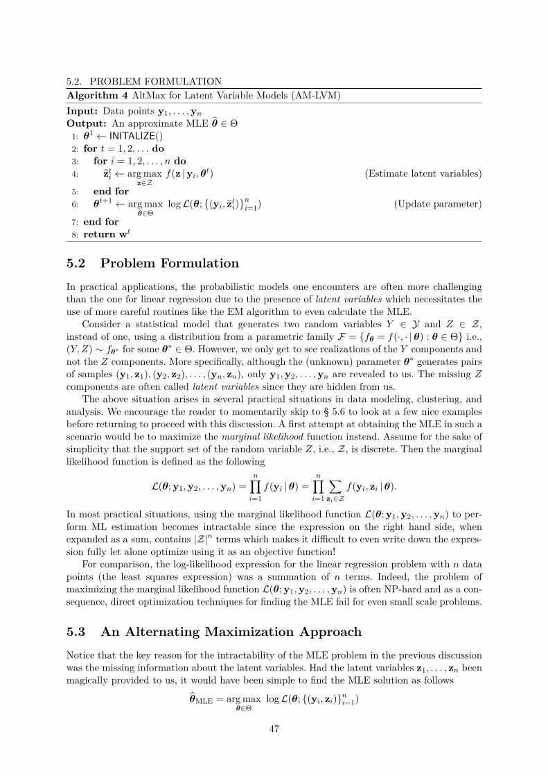
5.2. PROBLEM FORMULATIONAlgorithm 4 AltMax for Latent Variable Models (AM-LVM)Input: Data points y1, . . . ,ynOutput: An approximate MLE θ ∈ Θ1: θ1 ← INITALIZE()2: for t = 1, 2, . . . do3: for i = 1, 2, . . . , n do4: zti ← arg max
z∈Zf(z |yi,θt) (Estimate latent variables)
5: end for6: θt+1 ← arg max
θ∈ΘlogL(θ;
(yi, zti)
ni=1) (Update parameter)
7: end for8: return wt
5.2 Problem FormulationIn practical applications, the probabilistic models one encounters are often more challengingthan the one for linear regression due to the presence of latent variables which necessitates theuse of more careful routines like the EM algorithm to even calculate the MLE.
Consider a statistical model that generates two random variables Y ∈ Y and Z ∈ Z,instead of one, using a distribution from a parametric family F = fθ = f(·, · |θ) : θ ∈ Θ i.e.,(Y, Z) ∼ fθ∗ for some θ∗ ∈ Θ. However, we only get to see realizations of the Y components andnot the Z components. More specifically, although the (unknown) parameter θ∗ generates pairsof samples (y1, z1), (y2, z2), . . . , (yn, zn), only y1,y2, . . . ,yn are revealed to us. The missing Zcomponents are often called latent variables since they are hidden from us.
The above situation arises in several practical situations in data modeling, clustering, andanalysis. We encourage the reader to momentarily skip to § 5.6 to look at a few nice examplesbefore returning to proceed with this discussion. A first attempt at obtaining the MLE in such ascenario would be to maximize the marginal likelihood function instead. Assume for the sake ofsimplicity that the support set of the random variable Z, i.e., Z, is discrete. Then the marginallikelihood function is defined as the following
L(θ; y1,y2, . . . ,yn) =n∏i=1
f(yi |θ) =n∏i=1
∑zi∈Z
f(yi, zi |θ).
In most practical situations, using the marginal likelihood function L(θ; y1,y2, . . . ,yn) to per-form ML estimation becomes intractable since the expression on the right hand side, whenexpanded as a sum, contains |Z|n terms which makes it difficult to even write down the expres-sion fully let alone optimize using it as an objective function!
For comparison, the log-likelihood expression for the linear regression problem with n datapoints (the least squares expression) was a summation of n terms. Indeed, the problem ofmaximizing the marginal likelihood function L(θ; y1,y2, . . . ,yn) is often NP-hard and as a con-sequence, direct optimization techniques for finding the MLE fail for even small scale problems.
5.3 An Alternating Maximization ApproachNotice that the key reason for the intractability of the MLE problem in the previous discussionwas the missing information about the latent variables. Had the latent variables z1, . . . , zn beenmagically provided to us, it would have been simple to find the MLE solution as follows
θMLE = arg maxθ∈Θ
logL(θ; (yi, zi)ni=1)
47
CHAPTER 5. THE EM ALGORITHMHowever, notice that it is also true that, had the identity of the true parameter θ∗ been providedto us (again magically), it would have been simple to estimate the latent variables using amaximum posterior probability estimate for zi as follows
zi = arg maxz∈Z
f(z |yi,θ∗)
Given the above, it is tempting to apply a gAM-style algorithm to solve the MLE problem inthe presence of latent variables. Algorithm 4 outlines such an adaptation of gAM to the latentvariable learning problem. Note that steps 4 and 6 in the algorithm can be very efficientlycarried out for several problem cases. In fact, it can be shown2 that for the Gaussian Mixturemodeling problem, AM-LVM reduces to the popular Llyod’s algorithm for k-means clustering.
However, the AM-LVM algorithm has certain drawbacks, especially when the space of latentvariables Z is large. At every time step t, AM-LVM makes a “hard assignment”, assigning thedata point yi to just one value of the latent variable zti ∈ Z. This can amount to throwingaway a lot of information, especially when there may be other values z′ ∈ Z present such thatf(z′ |yi,θt) is also large but nevertheless f(z′ |yi,θt) < f(zti |yi,θt) so that AM-LVM neglectsz′. The EM algorithm tries to remedy this.
5.4 The EM Algorithm
Given the drawbacks of the hard assignment approach adopted by the AM-LVM algorithm, theEM algorithm presents an alternative approach that can be seen as making “soft” assignments.
At a very high level, the EM algorithm can be seen as doing the following. At time step t,instead of assigning the point yi to a single value of the latent variable zti = arg max
z∈Zf(z |yi,θt),
the EM algorithm chooses to make a partial assignment of yi to all possible values of the latentvariable in the set Z. The EM algorithm “assigns” yi to a value z ∈ Z with affinity/weightequal to f(z |yi,θt).
Thus, yi gets partially assigned to all possible values of the latent variable, to some withmore weight, to others with less weight. This avoids any loss of information. Note that theseweights are always positive and sum up to unity since
∑z∈Z f(z |yi,θt) = 1. Also note that
EM still assigns zti = arg maxz∈Z
f(z |yi,θt) the highest weight. In contrast, AM-LVM can be now
seen as putting all the weight on zti alone and zero weight on any other latent variable value.We now present a more formal derivation of the EM algorithm. Instead of maximizing the
likelihood in a single step, the EM algorithm tries to efficiently encourage an increase in thelikelihood over several steps. Define the point-wise likelihood function as
L(θ; y) =∑z∈Z
f(y, z |θ).
Note that we can write the marginal likelihood function as L(θ; y1,y2, . . . ,yn) =∏ni=1 L(θ; yi).
Our goal is to maximize L(θ; y1,y2, . . . ,yn) but doing so directly is too expensive. So the nextbest thing is to do so indirectly. Suppose we had a proxy function that lower bounded thelikelihood function but was also easy to optimize. Then maximizing the proxy function wouldalso lead to an increase in the likelihood if the proxy were really good.
This is the key to the EM algorithm: it introduces a proxy function called the Q-functionthat lower bounds the marginal likelihood function and casts the parameter estimation problemas a bi-variate problem, the two variables being the parameter θ and the Q-function.
2See Exercise 5.1.
48
5.4. THE EM ALGORITHMGiven an initialization, θ0 ∈ Θ, EM constructs a Q-function out of it, uses that as a proxy
to obtain a better parameter θ1, uses the newly obtained parameter to construct a better Q-function, uses the better Q-function to obtain a still better parameter θ2, and so on. Thus, itessentially performs alternating optimization steps, with better estimations of the θ parameterleading to better constructions of the Q-function and vice versa.
To formalize this notion, we will abuse notation to let f(z |y,θ0) denote the conditionalprobability function for the random variable Z given the variable Y and the parameter θ0.Then we have
logL(θ; y) = log∑z∈Z
f(y, z |θ) = log∑z∈Z
f(z |y,θ0) f(y, z |θ)f(z |y,θ0)
The summation in the last expression can be seen to be simply an expectation with respect tothe random variable Z being sampled from the conditional distribution f(· |y,θ0). Using this,we get
logL(θ; y) = logEz∼f(· |y,θ0)
[f(y, z |θ)f(z |y,θ0)
]
≥ Ez∼f(· |y,θ0)
[log f(y, z |θ)
f(z |y,θ0)
]= Ez∼f(· |y,θ0) [log f(y, z |θ)]︸ ︷︷ ︸
Qy(θ | θ0)
−Ez∼f(· |y,θ0)
[log f(z |y,θ0)
]︸ ︷︷ ︸
Ry(θ0)
.
The inequality follows from Jensen’s inequality as the logarithm function is concave. The func-tion Qy(θ |θ0) is called the point-wise Q-function. Now, the Q-function can be interpreted as aweighted point-wise likelihood function
Qy(θ |θ0) =∑z∈Z
wz · log f(y, z |θ),
with weights wz = f(z |y, θ0). Notice that this exactly corresponds to assigning y to everyz ∈ Z with weight wz instead of assigning it to just one value z = arg maxz∈Z f(z |y,θ0) (withweight 1) as AM-LVM does. We will soon see that due to the way the Q-function is used, theEM algorithm can be seen as performing AM-LVM with a soft-assignment step instead of ahard assignment step.
Using the point-wise Q-function, we define the Q-function.
Q(θ |θ0) = 1n
n∑i=1
Qyi(θ |θ0)
The Q-function has all the properties we desired from our proxy: parameters maximizingthe function Q(θ |θ0) do indeed improve the likelihood L(θ; y1,y2, . . . ,yn). More importantly,for several applications, it is possible to both construct as well as optimize the Q-function, veryefficiently.
Algorithm 5 gives an overall skeleton of the EM algorithm. Implementing EM requires tworoutines, one to construct the Q-function corresponding to the current iterate (the Expectationstep or E-step), and the other to maximize the Q-function (the Maximization step or M-step)to get the next iterate. We will next give precise constructions of these steps.
EM works well in many situations where the marginal likelihood function is inaccessible.This is because the Q-function only requires access to the conditional probability functionf(· |y,θ0) and the joint probability function f(·, · |θ), both of which are readily accessible inseveral applications. We will see examples of such applications shortly.
49
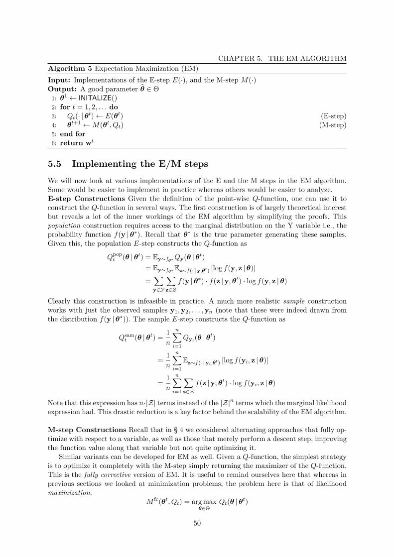
CHAPTER 5. THE EM ALGORITHMAlgorithm 5 Expectation Maximization (EM)Input: Implementations of the E-step E(·), and the M-step M(·)Output: A good parameter θ ∈ Θ1: θ1 ← INITALIZE()2: for t = 1, 2, . . . do3: Qt(· |θt)← E(θt) (E-step)4: θt+1 ←M(θt, Qt) (M-step)5: end for6: return wt
5.5 Implementing the E/M stepsWe will now look at various implementations of the E and the M steps in the EM algorithm.Some would be easier to implement in practice whereas others would be easier to analyze.E-step Constructions Given the definition of the point-wise Q-function, one can use it toconstruct the Q-function in several ways. The first construction is of largely theoretical interestbut reveals a lot of the inner workings of the EM algorithm by simplifying the proofs. Thispopulation construction requires access to the marginal distribution on the Y variable i.e., theprobability function f(y |θ∗). Recall that θ∗ is the true parameter generating these samples.Given this, the population E-step constructs the Q-function as
Qpopt (θ |θt) = Ey∼fθ∗Qy(θ |θt)
= Ey∼fθ∗Ez∼f(· |y,θt) [log f(y, z |θ)]
=∑y∈Y
∑z∈Z
f(y |θ∗) · f(z |y,θt) · log f(y, z |θ)
Clearly this construction is infeasible in practice. A much more realistic sample constructionworks with just the observed samples y1,y2, . . . ,yn (note that these were indeed drawn fromthe distribution f(y |θ∗)). The sample E-step constructs the Q-function as
Qsamt (θ |θt) = 1
n
n∑i=1
Qyi(θ |θt)
= 1n
n∑i=1
Ez∼f(· |yi,θt) [log f(yi, z |θ)]
= 1n
n∑i=1
∑z∈Z
f(z |y,θt) · log f(yi, z |θ)
Note that this expression has n·|Z| terms instead of the |Z|n terms which the marginal likelihoodexpression had. This drastic reduction is a key factor behind the scalability of the EM algorithm.
M-step Constructions Recall that in § 4 we considered alternating approaches that fully op-timize with respect to a variable, as well as those that merely perform a descent step, improvingthe function value along that variable but not quite optimizing it.
Similar variants can be developed for EM as well. Given a Q-function, the simplest strategyis to optimize it completely with the M-step simply returning the maximizer of the Q-function.This is the fully corrective version of EM. It is useful to remind ourselves here that whereas inprevious sections we looked at minimization problems, the problem here is that of likelihoodmaximization.
M fc(θt, Qt) = arg maxθ∈Θ
Qt(θ |θt)
50
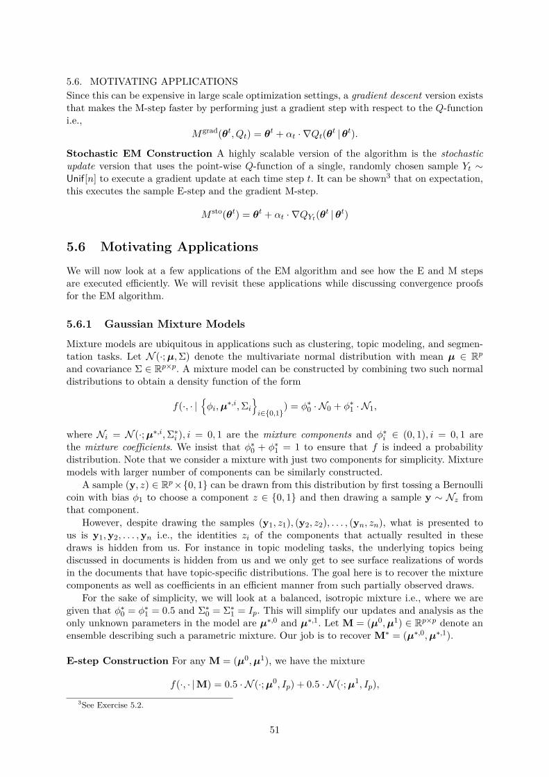
5.6. MOTIVATING APPLICATIONSSince this can be expensive in large scale optimization settings, a gradient descent version existsthat makes the M-step faster by performing just a gradient step with respect to the Q-functioni.e.,
Mgrad(θt, Qt) = θt + αt · ∇Qt(θt |θt).
Stochastic EM Construction A highly scalable version of the algorithm is the stochasticupdate version that uses the point-wise Q-function of a single, randomly chosen sample Yt ∼Unif[n] to execute a gradient update at each time step t. It can be shown3 that on expectation,this executes the sample E-step and the gradient M-step.
M sto(θt) = θt + αt · ∇QYt(θt |θt)
5.6 Motivating Applications
We will now look at a few applications of the EM algorithm and see how the E and M stepsare executed efficiently. We will revisit these applications while discussing convergence proofsfor the EM algorithm.
5.6.1 Gaussian Mixture Models
Mixture models are ubiquitous in applications such as clustering, topic modeling, and segmen-tation tasks. Let N (·; µ,Σ) denote the multivariate normal distribution with mean µ ∈ Rpand covariance Σ ∈ Rp×p. A mixture model can be constructed by combining two such normaldistributions to obtain a density function of the form
f(·, · |φi,µ
∗,i,Σi
i∈0,1
) = φ∗0 · N0 + φ∗1 · N1,
where Ni = N (·; µ∗,i,Σ∗i ), i = 0, 1 are the mixture components and φ∗i ∈ (0, 1), i = 0, 1 arethe mixture coefficients. We insist that φ∗0 + φ∗1 = 1 to ensure that f is indeed a probabilitydistribution. Note that we consider a mixture with just two components for simplicity. Mixturemodels with larger number of components can be similarly constructed.
A sample (y, z) ∈ Rp×0, 1 can be drawn from this distribution by first tossing a Bernoullicoin with bias φ1 to choose a component z ∈ 0, 1 and then drawing a sample y ∼ Nz fromthat component.
However, despite drawing the samples (y1, z1), (y2, z2), . . . , (yn, zn), what is presented tous is y1,y2, . . . ,yn i.e., the identities zi of the components that actually resulted in thesedraws is hidden from us. For instance in topic modeling tasks, the underlying topics beingdiscussed in documents is hidden from us and we only get to see surface realizations of wordsin the documents that have topic-specific distributions. The goal here is to recover the mixturecomponents as well as coefficients in an efficient manner from such partially observed draws.
For the sake of simplicity, we will look at a balanced, isotropic mixture i.e., where we aregiven that φ∗0 = φ∗1 = 0.5 and Σ∗0 = Σ∗1 = Ip. This will simplify our updates and analysis as theonly unknown parameters in the model are µ∗,0 and µ∗,1. Let M = (µ0,µ1) ∈ Rp×p denote anensemble describing such a parametric mixture. Our job is to recover M∗ = (µ∗,0,µ∗,1).
E-step Construction For any M = (µ0,µ1), we have the mixture
f(·, · |M) = 0.5 · N (·; µ0, Ip) + 0.5 · N (·; µ1, Ip),3See Exercise 5.2.
51
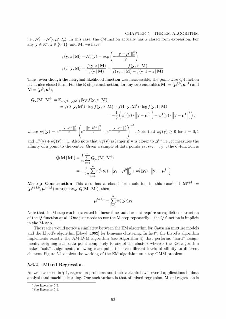
CHAPTER 5. THE EM ALGORITHMi.e., Ni = N (·; µi, Ip). In this case, the Q-function actually has a closed form expression. Forany y ∈ Rp, z ∈ 0, 1, and M, we have
f(y, z |M) = Nz(y) = exp(−‖y− µz‖22
2
)
f(z |y,M) = f(y, z |M)f(y |M) = f(y, z |M)
f(y, z |M) + f(y, 1− z |M) .
Thus, even though the marginal likelihood function was inaccessible, the point-wise Q-functionhas a nice closed form. For the E-step construction, for any two ensembles Mt = (µt,0,µt,1) andM = (µ0,µ1),
Qy(M |Mt) = Ez∼f(· |y,Mt) [log f(y, z |M)]= f(0 |y,Mt) · log f(y, 0 |M) + f(1 |y,Mt) · log f(y, 1 |M)
= −12
(w0t (y) ·
∥∥∥y− µ0∥∥∥2
2+ w1
t (y) ·∥∥∥y− µ1
∥∥∥2
2
),
where wzt (y) = e−‖y−µt,z‖2
22
e−‖y−µt,0‖22
2 + e−‖y−µt,1‖2
22
−1
. Note that wzt (y) ≥ 0 for z = 0, 1
and w0t (y) +w1
t (y) = 1. Also note that wzt (y) is larger if y is closer to µt,z i.e., it measures theaffinity of a point to the center. Given a sample of data points y1,y2, . . . ,yn, the Q-function is
Q(M |Mt) = 1n
n∑i=1
Qyi(M |Mt)
= − 12n
n∑i=1
w0t (yi) ·
∥∥∥yi − µ0∥∥∥2
2+ w1
t (yi) ·∥∥∥yi − µ1
∥∥∥2
2
M-step Construction This also has a closed form solution in this case4. If Mt+1 =(µt+1,0,µt+1,1) = arg maxM Q(M |Mt), then
µt+1,z =n∑i=1
wzt (yi)yi
Note that the M-step can be executed in linear time and does not require an explicit constructionof the Q-function at all! One just needs to use the M-step repeatedly – the Q-function is implicitin the M-step.
The reader would notice a similarity between the EM algorithm for Gaussian mixture modelsand the Llyod’s algorithm [Lloyd, 1982] for k-means clustering. In fact5, the Llyod’s algorithmimplements exactly the AM-LVM algorithm (see Algorithm 4) that performs “hard” assign-ments, assigning each data point completely to one of the clusters whereas the EM algorithmmakes “soft” assignments, allowing each point to have different levels of affinity to differentclusters. Figure 5.1 depicts the working of the EM algorithm on a toy GMM problem.
5.6.2 Mixed Regression
As we have seen in § 1, regression problems and their variants have several applications in dataanalysis and machine learning. One such variant is that of mixed regression. Mixed regression is
4See Exercise 5.3.5See Exercise 5.1.
52
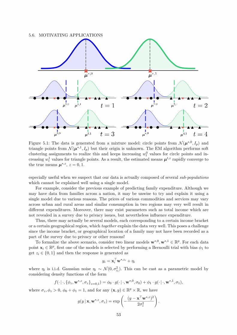
5.6. MOTIVATING APPLICATIONS
Figure 5.1: The data is generated from a mixture model: circle points from N (µ∗,0, Ip) andtriangle points from N (µ∗,1, Ip) but their origin is unknown. The EM algorithm performs softclustering assignments to realize this and keeps increasing w0
t values for circle points and in-creasing w1
t values for triangle points. As a result, the estimated means µt,z rapidly converge tothe true means µ∗,z, z = 0, 1.
especially useful when we suspect that our data is actually composed of several sub-populationswhich cannot be explained well using a single model.
For example, consider the previous example of predicting family expenditure. Although wemay have data from families across a nation, it may be unwise to try and explain it using asingle model due to various reasons. The prices of various commodities and services may varyacross urban and rural areas and similar consumption in two regions may very well result indifferent expenditures. Moreover, there may exist parameters such as total income which arenot revealed in a survey due to privacy issues, but nevertheless influence expenditure.
Thus, there may actually be several models, each corresponding to a certain income bracketor a certain geographical region, which together explain the data very well. This poses a challengesince the income bracket, or geographical location of a family may not have been recorded as apart of the survey due to privacy or other reasons!
To formalize the above scenario, consider two linear models w∗,0,w∗,1 ∈ Rp. For each datapoint xi ∈ Rp, first one of the models is selected by performing a Bernoulli trial with bias φ1 toget zi ∈ 0, 1 and then the response is generated as
yi = x>i w∗,zi + ηi
where ηi is i.i.d. Gaussian noise ηi ∼ N (0, σ2zi). This can be cast as a parametric model by
considering density functions of the form
f(· | ·, φz,w∗,z, σzz=0,1) = φ0 · g(· | ·,w∗,0, σ0) + φ1 · g(· | ·,w∗,1, σ1),
where σz, φz > 0, φ0 + φ1 = 1, and for any (x, y) ∈ Rp × R, we have
g(y |x,w∗,z, σz) = exp(−(y − x>w∗,z)2
2σ2z
).
53
CHAPTER 5. THE EM ALGORITHMNote that although such a model generates data in the form of triplets(x1, y1, z1), (x2, y2, z2), . . . , (xn, yn, zn), we are only allowed to observe(x1, y1), (x2, y2), . . . , (xn, yn) as the data. For the sake of simplicity, we will yet againlook at the special case when the Bernoulli trials are fair i.e., φ0 = φ1 = 0.5 and σ1 = σ2 = 1.Thus, the only unknown parameters are the models w∗,0 and w∗,1. Let W = (w0,w1) ∈ Rp×pdenote the parametric mixed model. Our job is to recover W∗ = (w∗,0,w∗,1).
A particularly interesting special case arises when we further impose the constraint w∗,0 =−w∗,1, i.e. the two models in the mixture are tied together to be negative of each other. Thismodel is especially useful in the phase retrieval problem. Although we will study this problemin more generality in § 10, we present a special case here.
Phase retrieval is a problem that arises in several imaging situations such as X-ray crys-tallography where, after data (xi, yi)i=1,...,n has been generated as yi = 〈w∗,xi〉, the sign ofthe response (or more generally, the phase of the response if the response is complex-valued)is omitted and we are presented with just (xi, |yi|)i=1,...,n. In such a situation, we can usethe latent variable zi = sign(yi) to denote the omitted sign information. In this setting, it canbe seen that the mixture model with w∗,0 = −w∗,1 is very appropriate since each data point(xi, |yi|) will be nicely explained by either w∗ or −w∗ depending on the value of sign(yi).
We will revisit this problem in detail in § 10. For now we move on to discuss the E andM-step constructions for the mixed regression problem. We leave details of the constructionsas an exercise6.
E-step Construction The point-wise Q-function has a closed form expression. Given twoensembles Wt = (wt,0,wt,1) and W = (w0,w1),
Q(x,y)(W|Wt) = −12(α0t,(x,y) · (y − x>w0)2 − α1
t,(x,y) · (y − x>w1)2),
where αzt,(x,y) = e−(y−x>wt,z)2
2
[e−
(y−x>wt,0)22 + e−
(y−x>wt,1)22
]−1. Note that αzt,(x,y) ≥ 0 for
z = 0, 1 and α0t,(x,y) + α1
t,(x,y) = 1. Also note that αzt,(x,y) is larger if wt,z gives less regressionerror for the point (x, y) than wt,1−z i.e., if (y − x>wt,z)2 < (y − x>wt,1−z)2. Thus, thedata point (x, y) feels greater affinity to the model that fits it better, which is intuitively, anappropriate thing to do.
M-step Construction The maximizer of the Q-function has a closed form solution in thiscase as well. If Wt+1 = (wt+1,0,wt+1,1) = arg maxWQ(W|Wt), where Q(W|Wt) is the sampleQ-function created from a data sample (x1, y1), (x2, y2), . . . , (xn, yn), then it is easy to see thatthe M-step update is given by the solution to two weighted least squares problems with weightsgiven by αzt,(xi,yi) for z = 0, 1, which have closed form solutions given by
wt+1,z =(
n∑i=1
αzt,(xi,yi) · xix>i
)−1 n∑i=1
αzt,(xi,yi) · yixi
Note that to update wt,0, for example, the M-step essentially performs least squares only overthose points (xi, yi) such that α0
t,(x,y) is large and ignores points where α0t,(x,y) ≈ 0. This is
akin to identifying points that belong to sub-population 0 strongly and performing regressiononly over them. One need not construct the Q-function explicitly here either and may simplykeep repeating the M-step. Figure 5.2 depicts the working of the EM algorithm on a toy mixedregression problem.
6See Exercise 5.4.
54
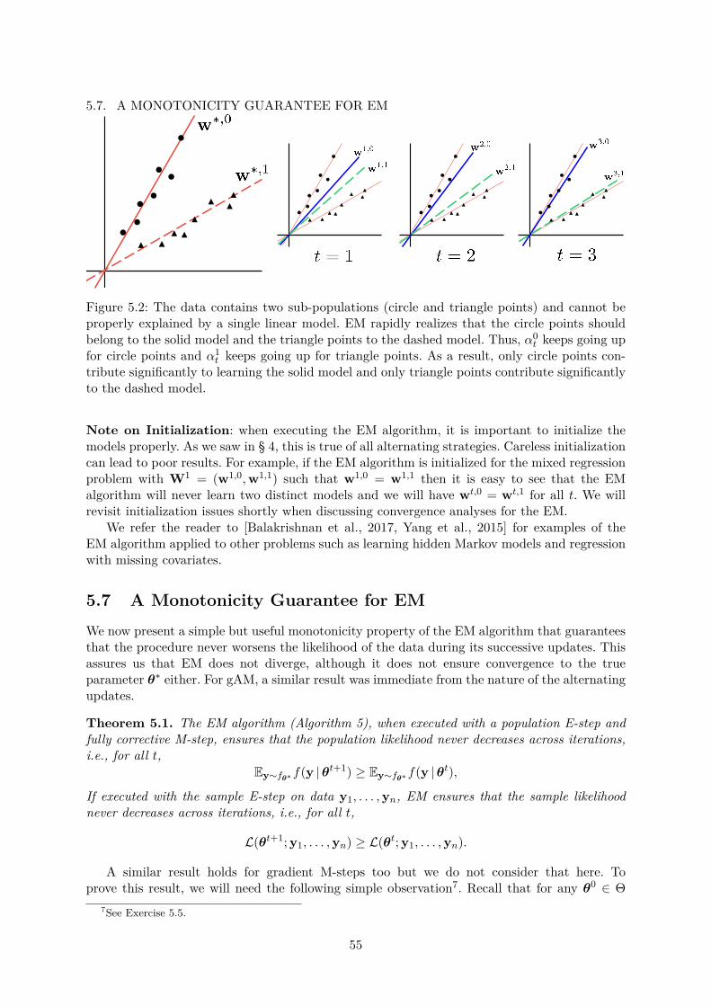
5.7. A MONOTONICITY GUARANTEE FOR EM
Figure 5.2: The data contains two sub-populations (circle and triangle points) and cannot beproperly explained by a single linear model. EM rapidly realizes that the circle points shouldbelong to the solid model and the triangle points to the dashed model. Thus, α0
t keeps going upfor circle points and α1
t keeps going up for triangle points. As a result, only circle points con-tribute significantly to learning the solid model and only triangle points contribute significantlyto the dashed model.
Note on Initialization: when executing the EM algorithm, it is important to initialize themodels properly. As we saw in § 4, this is true of all alternating strategies. Careless initializationcan lead to poor results. For example, if the EM algorithm is initialized for the mixed regressionproblem with W1 = (w1,0,w1,1) such that w1,0 = w1,1 then it is easy to see that the EMalgorithm will never learn two distinct models and we will have wt,0 = wt,1 for all t. We willrevisit initialization issues shortly when discussing convergence analyses for the EM.
We refer the reader to [Balakrishnan et al., 2017, Yang et al., 2015] for examples of theEM algorithm applied to other problems such as learning hidden Markov models and regressionwith missing covariates.
5.7 A Monotonicity Guarantee for EMWe now present a simple but useful monotonicity property of the EM algorithm that guaranteesthat the procedure never worsens the likelihood of the data during its successive updates. Thisassures us that EM does not diverge, although it does not ensure convergence to the trueparameter θ∗ either. For gAM, a similar result was immediate from the nature of the alternatingupdates.
Theorem 5.1. The EM algorithm (Algorithm 5), when executed with a population E-step andfully corrective M-step, ensures that the population likelihood never decreases across iterations,i.e., for all t,
Ey∼fθ∗f(y |θt+1) ≥ Ey∼fθ∗f(y |θt),
If executed with the sample E-step on data y1, . . . ,yn, EM ensures that the sample likelihoodnever decreases across iterations, i.e., for all t,
L(θt+1; y1, . . . ,yn) ≥ L(θt; y1, . . . ,yn).
A similar result holds for gradient M-steps too but we do not consider that here. Toprove this result, we will need the following simple observation7. Recall that for any θ0 ∈ Θ
7See Exercise 5.5.
55
CHAPTER 5. THE EM ALGORITHMand y ∈ Y, we defined the terms Qy(θ |θ0) = E
z∼f(· |y,θ0)[log f(y, z |θ)] and Ry(θ0) =
Ez∼f(· |y,θ0)
[log f(z |y,θ0)
].
Lemma 5.2. For any θ0 ∈ Θ, we have
log f(y |θ0) = Qy(θ0 |θ0)−Ry(θ0)
This is a curious result since we have earlier seen that for any θ ∈ Θ, we have the inequalitylog f(y |θ) ≥ Qy(θ |θ0)− Ry(θ0) by an application of the Jensen’s inequality (see § 5.4). Theabove lemma suggests that the inequality is actually tight. We now prove Theorem 5.1.
Proof (of Theorem 5.1). Consider the sample E-step with Q(θ |θt) = 1n
∑ni=1Qyi(θ |θt). A sim-
ilar argument works for population E-steps. The fully corrective M-step ensures Q(θt+1 |θt) ≥Q(θt |θt) i.e.,
1n
n∑i=1
Qyi(θt+1 |θt) ≥ 1n
n∑i=1
Qyi(θt |θt).
Subtracting the same terms from both sides gives us
1n
n∑i=1
(Qyi(θt+1 |θt)−Ryi(θt)
)≥ 1n
n∑i=1
(Qyi(θt |θt)−Ryi(θt)
).
Using the inequality log f(y |θt+1) ≥ Qy(θt+1 |θ0)−Ry(θ0) and applying Lemma 5.2 gives us
1n
n∑i=1
log f(yi |θt+1) ≥ 1n
n∑i=1
log f(yi |θt),
which proves the result.
5.8 Local Strong Concavity and Local Strong SmoothnessIn order to prove stronger convergence guarantees for the EM algorithm, we need to introducea few structural properties of parametric distributions. Let us recall the EM algorithm with apopulation E-step and fully corrective M-step for sake of simplicity.
1. (E-step) Q(· |θt) = Ey∼fθ∗Qy(· |θt)
2. (M-step) θt+1 = arg maxθ∈Θ
Qt(θ |θt)
For any θ0 ∈ Θ, we will use qθ0(·) = Q(· |θ0) as a shorthand for the Q-function with respect toθ0 (constructed at the population or sample level depending on the E-step) and let M(θ0) :=arg max
θ∈Θqθ0(θ) denote the output of the M-step if θ0 is the current parameter. Let θ∗ denote a
parameter that optimizes the population likelihood
θ∗ ∈ arg maxθ∈Θ
Ey∼f(y|θ∗)
[L(θ; y)] = arg maxθ∈Θ
Ey∼f(y|θ∗)
[f(y |θ)]
Recall that our overall goal is indeed to recover a parameter such as θ∗ that maximizes thepopulation level likelihood (or else sample likelihood if using sample E-steps). Now the Q-function satisfies8 the following self-consistency property.
θ∗ ∈ arg maxθ∈Θ
qθ∗(θ)
8See Exercise 5.6.
56
5.8. LOCAL STRONG CONCAVITY AND LOCAL STRONG SMOOTHNESSThus, if we could somehow get hold of the Q-function qθ∗(·), then a single M-step would solvethe problem! However, this is a circular argument since getting hold of qθ∗(·) would requirefinding θ∗ first.
To proceed along the previous argument, we need to refine this observation. Not only shouldthe M-step refuse to deviate from the optimum θ∗ if initialized there, it should behave inrelatively calm manner in the neighborhood of the optimum as well. The following propertiescharacterize “nice” Q functions that ensure this happens.
For sake of simplicity, we will assume that all Q-functions are continuously differentiable,as well as that the estimation problem is unconstrained i.e., Θ = Rp. Note that this ensures∇qθ∗(θ∗) = 0 due to self-consistency. Also note that since we are looking at maximizationproblems, we will require the Q function to satisfy “concavity” properties instead of “convexity”properties.
Definition 5.1 (Local Strong Concavity). A statistical estimation problem with a populationlikelihood maximizer θ∗ satisfies the (r, α)-Local Strong Concavity (LSC) property if there existα, r > 0, such that the function qθ∗(·) is α-strongly concave in neighborhood ball of radius raround θ∗ i.e., for all θ1,θ2 ∈ B2(θ∗, r),
qθ∗(θ1)− qθ∗(θ2)−⟨∇qθ∗(θ2),θ1 − θ2
⟩≤ −α2
∥∥∥θ1 − θ2∥∥∥2
2
The reader would find LSC similar to restricted strong convexity (RSC) in Definition 3.2,with the “restriction” being the neighborhood B2(θ∗, r) of θ∗. Also note that only qθ∗(·) isrequired to satisfy the LSC property, and not Q-functions corresponding to every θ.
We will also require a counterpart to restricted strong smoothness (RSS). For that, weintroduce the notion of Lipschitz gradients.
Definition 5.2 (Lipschitz Gradients). A differentiable function f : Rp → R is said to haveβ-Lipschitz gradients if for all x,y ∈ Rp, we have
‖∇f(x)−∇f(y)‖2 ≤ β · ‖x− y‖2 .
We advise the reader to relate this notion to that of Lipschitz functions (Definition 2.5).It can be shown9 that all functions with L-Lipschitz gradients are also L-strongly smooth(Definition 2.4). Using this notion we are now ready to introduce our next properties.
Definition 5.3 (Local Strong Smoothness). A statistical estimation problem with a populationlikelihood maximizer θ∗ satisfies the (r, β)-Local Strong Smoothness (LSS) property if there existβ, r > 0, such that for all θ1,θ2 ∈ B2(θ∗, r), the function qθ∗(·) satisfies∥∥∥∇qθ∗(M(θ1))−∇qθ∗(M(θ2))
∥∥∥2≤ β ·
∥∥∥θ1 − θ2∥∥∥
2
The above property ensures that in the restricted neighborhood around the optimum, the Q-function qθ∗(·) is strongly smooth. The similarity to RSS is immediate. Note that this propertyalso generalizes the self-consistency property we saw a moment ago.
Self-consistency forces ∇qθ∗(θ∗) = 0 at the optimum. LSS forces such behavior to extendaround the optimum as well. To see this, simply set θ2 = θ∗ with LSS and observe the corollary∥∥∥∇qθ∗(M(θ1))
∥∥∥2≤ β ·
∥∥∥θ1 − θ∗∥∥∥
2. The curious reader may wish to relate this corollary to the
Robust Bistability property (Definition 4.6) and the Local Error Bound property introduced byLuo and Tseng [1993].
The LSS property offers, as another corollary, a useful property of statistical estimationproblems called the First Order Stability property (introduced by Balakrishnan et al. [2017] ina more general setting).
9See Exercise 5.7.
57
CHAPTER 5. THE EM ALGORITHMDefinition 5.4 (First Order Stability [Balakrishnan et al., 2017]). A statistical estimationproblem with a population likelihood maximizer θ∗ satisfies the (r, γ)-First Order Stability (FOS)property if there exist γ > 0, r > 0 such that the the gradients of the functions qθ(·) are stablein a neighborhood of θ∗ i.e., for all θ ∈ B2(θ∗, r),
‖∇qθ(M(θ))−∇qθ∗(M(θ))‖2 ≤ γ · ‖θ − θ∗‖2
Lemma 5.3. A statistical estimation problem that satisfies the (r, β)-LSS property, also satisfiesthe (r, β)-FOS property.
Proof. Since M(θ) maximizes the function qθ(·) due to the M-step, and the problem is uncon-strained and the Q-functions differentiable, we get ∇qθ(M(θ)) = 0. Thus, we have, using thetriangle inequality,
‖∇qθ(M(θ))−∇qθ∗(M(θ))‖2 = ‖∇qθ∗(M(θ))‖2≤ ‖∇qθ∗(M(θ))−∇qθ∗(M(θ∗))‖2 + ‖∇qθ∗(M(θ∗))‖2≤ β · ‖θ − θ∗‖2 ,
using self-consistency to get M(θ∗) = θ∗ and ∇qθ∗(θ∗) = 0.
5.9 A Local Convergence Guarantee for EMWe will now prove a convergence result much stronger than Theorem 5.1: if EM is initialized“close” to the optimal parameter θ∗ for “nice” problems, then it approaches θ∗ at a linear rate.For the sake of simplicity, we will analyze EM with population E-steps and fully correctiveM-steps. We refer the reader to [Balakrishnan et al., 2017] for analyses of sample E-steps andstochastic M-steps. The following contraction lemma will be crucial in the analysis of the EMalgorithm.
Lemma 5.4. Suppose we have a statistical estimation problem with a population likelihoodmaximizer θ∗ that, for some α, β, r > 0, satisfies the (r, α)-LSC and (r, β)-LSS properties.Then in the region B2(θ∗, r), the M operator corresponding to the fully corrective M-step iscontractive, i.e., for all θ ∈ B2(θ∗, r),
‖M(θ)−M(θ∗)‖2 ≤β
α· ‖θ − θ∗‖2
Since by the self consistency property, we have M(θ∗) = θ∗ and the EM algorithm setsθt+1 = M(θt) due to the M-step, Lemma 5.4 immediately guarantees the following local con-vergence property10.
Theorem 5.5. Suppose a statistical estimation problem with population likelihood maximizerθ∗ satisfies the (r, α)-LSC and (r, β)-LSS properties such that β < α. Let the EM algorithm(Algorithm 5) be initialized with θ1 ∈ B2(θ∗, r) and executed with population E-steps and fullycorrective M-steps. Then after at most T = O
(log 1
ε
)steps, we have
∥∥θt − θ∗∥∥
2 ≤ ε.
Note that the above result holds only if β < α, in other words, if the condition numberκ = β/α < 1. We hasten to warn the reader that whereas in previous sections we always hadκ ≥ 1, here the LSC and LSS properties are defined differently (LSS involves the M-step whereasLSC does not) and thus it is possible that we have κ < 1.
10See Exercise 5.8.
58
5.9. A LOCAL CONVERGENCE GUARANTEE FOR EMAlso, since all functions satisfy (0, 0)-LSC, it is plausible that for well behaved problems, even
for α > β, there should exist some small radius r(α) so that the (r(α), α)-LSC property holds.This may require the EM algorithm to be initialized closer to the optimum for the convergenceproperties to kick in. We now prove Lemma 5.4 below.
Proof of Lemma 5.4. Since we have differentiable Q-functions and an unconstrained estimationproblem, we immediately get a lot of useful results. We note that this lemma holds even forconstrained estimation problems but the arguments are more involved which we wish to avoid.Let θ ∈ B2(θ∗, r) be any parameter in the r-neighborhood of θ∗.
(Apply Local Strong Concavity) Upon a two sided application of LSC and using∇qθ∗(θ∗) =0, we get
qθ∗(θ∗)− qθ∗(M(θ))− 〈∇qθ∗(M(θ)),θ∗ −M(θ)〉 ≤ −α2 ‖M(θ)− θ∗‖22
qθ∗(M(θ))− qθ∗(θ∗) ≤ −α
2 ‖θ∗ −M(θ)‖22 ,
adding which gives us the inequality
〈∇qθ∗(M(θ)),θ∗ −M(θ)〉 ≥ α · ‖M(θ)− θ∗‖22
(Apply Local Strong Smoothness) Since M(θ) maximizes the function qθ(·) due to theM-step, we get ∇qθ(M(θ)) = 0. Thus,
〈∇qθ∗(M(θ)),θ∗ −M(θ)〉 = 〈∇qθ∗(M(θ))−∇qθ(M(θ)),θ∗ −M(θ)〉≤ ‖∇qθ∗(M(θ))−∇qθ(M(θ))‖2 ‖θ
∗ −M(θ)‖2
Using Lemma 5.3 to invoke the (r, β)-FOS property further gives us
〈∇qθ∗(M(θ)),θ∗ −M(θ)〉 ≤ β · ‖θ − θ∗‖2 ‖θ∗ −M(θ)‖2
Combining the two results proved above gives us
α · ‖M(θ)− θ∗‖22 ≤ β · ‖M(θ)− θ∗‖2 · ‖θ − θ∗‖2 ,
which finish the proof.
5.9.1 A Note on the Application of Convergence Guarantees
We conclude the discussion with some comments on the feasibility of the structural assumptionswe used to prove the convergence guarantees, in practical settings. Rigorous proofs that theseproperties are indeed satisfied in practical applications is beyond the scope of this monograph.These can be found in [Balakrishnan et al., 2017]. Note that for the convergence guarantees(specifically Lemma 5.4) to hold, a problem need only satisfy the LSC and FOS properties,with LSS being equivalent to FOS due to Lemma 5.3.
Gaussian Mixture Models To analyze the LSC and FOS properties, we need to look at thepopulation version of the Q-function. Given the point-wise Q-function derivation of the in § 5.6,we get for M = (µ0,µ1)
Q(M |M∗) = −12Ey∼fM∗
[w0(y) ·
∥∥∥y− µ0∥∥∥2
2+ w1(y) ·
∥∥∥y− µ1∥∥∥2
2
],
59
CHAPTER 5. THE EM ALGORITHM
where wz(y) = e−‖y−µ∗,z‖2
22
e−‖y−µ∗,0‖22
2 + e−‖y−µ∗,1‖2
22
−1
for z = 0, 1. It can be seen that the
function qM∗(·) satisfies ∇2qM∗(·) w · I where w = minE[w0(y)
],E[w1(y)
]> 0 and hence
this problem satisfies the (∞, w)-LSC property i.e., it is globally strongly concave.Establishing the FOS property is more involved. However, it can be shown that the problem
does satisfy the (r, α)-FOS property with r = Ω(‖M∗‖2) and α = exp(−Ω(‖M∗‖22
)) under
suitable conditions.
Mixed Regression We again use the point-wise Q-function construction to construct thepopulation Q-function. For any W = (w0,w1),
Q(x,y)(W|W∗) = −12E[α0
(x,y) · (y − x>w0)2 − α1(x,y) · (y − x>w1)2
],
where αz(x,y) = e−(y−x>w∗,z)2
2
[e−
(y−x>w∗,0)22 + e−
(y−x>w∗,1)22
]−1. Assuming
E[xx>
]= I for sake of simplicity, we get ∇2qW∗(·) α · I where α =
minλmin
(E[w0(x, y) · xx>
]), λmin
(E[w1(x, y) · xx>
])i.e., the problem satisfies the
(∞, w)-LSC property i.e., it is globally strongly concave. Establishing the FOS property ismore involved but the problem does satisfy the (r, α)-FOS property with r = Ω(‖W∗‖2) andα = Ω (1) under suitable conditions.
5.10 ExercisesExercise 5.1. Show that for Gaussian mixture models with a balanced isotropic mixture, theAM-LVM algorithm (Algorithm 4) implements exactly recovers Lloyd’s algorithm for k-meansclustering. Note that AM-LVM in this case prescribes setting w0
t (y) = 1 if∥∥y− µt,0∥∥
2 ≤∥∥y− µt,1∥∥2 and 0 otherwise and also setting w1
t (y) = 1− w0t (y).
Exercise 5.2. Show that on expectation, the stochastic EM update rule is, on expectation, equiv-alent to the sample E and the gradient M-step i.e., E
[M sto(θt, Qt) |θt
]= M grad(θt, Qsam
t (· |θt)).Exercise 5.3. Derive the fully corrective and gradient M-step in the Gaussian mixture modelingproblem. Show that they have closed forms.Exercise 5.4. Derive the E and M-step constructions for the mixed regression problem withfair Bernoulli trials.Exercise 5.5. Prove Lemma 5.2.Exercise 5.6. Let θ be a population likelihood maximizer i.e.,
θ ∈ arg maxθ∈Θ
Ey∼f(y|θ∗)
[f(y |θ)]
Then show that θ ∈ arg maxθ∈Θ
qθ(θ). Hint: One way to show this result is to use Theorem 5.1
and Lemma 5.2.Exercise 5.7. Show that a function f (whether convex or not) that has L-Lipschitz gradientsis necessarily L-strongly smooth. Also show that for any given L > 0, there exist functions thatdo not have L-Lipschitz gradients which are also not L-strongly smooth.Hint: Use the fundamental theorem for calculus for line integrals for the first part. For the secondpart try using a quadratic function.
60
5.11. BIBLIOGRAPHIC NOTESExercise 5.8. For any statistical estimation problem with population likelihood maximizer θ∗
that satisfies the LSC and LSS properties with appropriate constants, show that parametersclose to θ∗ are approximate population likelihood maximizers themselves. Show this by findingconstants ε0, D > 0 (that may depend on the LSC, LSS constants) such that for any θ, if‖θ − θ∗‖2 ≤ ε < ε0, then
Ey∼f(y|θ∗)
[f(y |θ)] ≥ Ey∼f(y|θ∗)
[f(y |θ∗)]−D · ε.
Hint: Use Lemma 5.2 and Exercise 5.7.Exercise 5.9. Similar to how the EM algorithm ensures monotone progress with respect to thelikelihood objective (see § 5.7), show that the the AM-LVM algorithm (see Algorithm 4) ensuresmonotone progress with respect to the following optimization problem
maxθ∈Θ
zi,...,zn∈Z
L (θ; (yi, zi)ni=1) .
More specifically, show that if the iterates obtained by AM-LVM at time t are θt,ztini=1, then
we have for all t ≥ 1
L(θt+1;
(yi, zt+1
i )ni=1
)≥ L
(θt;
(yi, zti)ni=1
)5.11 Bibliographic NotesThe EM algorithm was given its name and formally introduced in the seminal work of Dempsteret al. [1977]. Although several results exist that attempt to characterize the convergence prop-erties of the EM algorithm, prominent among them is the work of Wu [1983] which showed thatfor problems with a uni-modal likelihood function and some regularity conditions that make theestimation problem well-posed, the EM algorithm converges to the (unique) global optimum.
We have largely followed the work of Balakrishnan et al. [2017] in the treatment of thetopic in this section. Recent results have attempted to give local convergence results for theEM algorithm, similar to the ones we discussed. Examples include analyses of the Baum-Welchalgorithm used to learn hidden Markov models [Yang et al., 2015], the EM algorithm [Balakrish-nan et al., 2017], and the more general problem of M-estimation [Andresen and Spokoiny, 2016](recall that maximum likelihood estimators are members of the broader class of M-estimators).The recurring message here is that upon proper initialization, the EM algorithm does convergeto the global optimum.
For certain problems, such as mixed regression, it is known how to get such initializations inpolynomial time under regularity assumptions [Yi et al., 2014] which makes the entire procedurea polynomial time solution to get globally consistent parameters. Other recent advances inthe area include extensions to high dimensional estimation estimation problems by way ofregularization [Yi and Caramanis, 2015] or directly incorporating sparsity structure into theprocedure [Wang et al., 2015]. We refer the reader to the work of Balakrishnan et al. [2017] andother more recent works for a more detailed review of literature in this area.
As a closing note, we reiterate our previous comment on similarities between EM and alter-nating minimization. Both have an alternating pattern in their execution with each alternationtypically being cheap and easy to execute. Indeed, for several areas in which the EM approachhas been found successful, such as learning mixture models, regression with missing or corrupteddata, phase retrieval etc, there also exist efficient alternating minimization algorithms. We willlook at some of them in later sections. Having said that, the EM algorithm does distinguish itselfwithin the general alternating minimization approach in its single minded goal of approachingthe MLE by promoting parameters that increase the likelihood of the data.
61
The official publication is available from now publishers viahttp://dx.doi.org/10.1561/2200000058
Chapter 6
Stochastic Optimization Techniques
In previous sections, we have looked at specific instances of optimization problems with non-convex objective functions. In § 4 we looked at problems in which the objective can be expressedas a function of two variables, whereas in § 5 we looked at objective functions with latentvariables that arose in probabilistic settings. In this section, we will look at the problem ofoptimization with non-convex objectives in a more general setting.
Several machine learning and signal processing applications such as deep learning, topicmodeling etc, generate optimization problems that have non-convex objective functions. Theglobal optimization of non-convex objectives, i.e., finding the global optimum of the objectivefunction, is an NP hard problem in general. Even the seemingly simple problem of minimizingquadratic functions of the kind x>Ax over convex constraint sets becomes NP-hard the momentthe matrix A is allowed to have even one negative eigenvalue.
As a result, a much sought after goal in applications with non-convex objectives is to find alocal minimum of the objective function. The main hurdle in achieving local optimality is thepresence of saddle points which can mislead optimization methods such as gradient descent bystalling their progress. Saddle points are best avoided as they signal inflection in the objectivesurface and unlike local optima, they need not optimize the objective function in any meaningfulway.
The recent years have seen much interest in this problem, particularly with the advent ofdeep learning where folklore wisdom tells us that in the presence of sufficient data, even locallyoptimal solutions to the problem of learning the edge weights of a network perform quite well[Choromanska et al., 2015]. In these settings, techniques such as convex relaxations, and non-convex optimization techniques that we have studied such as EM, gAM, gPGD, do not applydirectly. In these settings, one has to attempt optimizing a non-convex objective directly.
The problem of avoiding or escaping saddle points is actually quite challenging in itselfgiven the wide variety of configurations saddle points can appear in, especially in high dimen-sional problems. It should be noted that there exist saddle configurations, bypassing which isintractable in itself. For such cases, even finding locally optimal solutions is an NP-hard problem[Anandkumar and Ge, 2016].
In our discussion, we will look recent results which show that if the function being optimizedpossesses certain nice structural properties, then an application of very intuitive algorithmictechniques can guarantee local optimality of the solutions. This will be yet another instance ofa result where the presence of a structural property (such as RSC/RSS, MSC/MSS, or LSC/LSSas studied in previous sections) makes the problem well behaved and allows efficient algorithmsto offer provably good solutions. Our discussion will largely aligned to the work of Ge et al.[2015]. The bibliographic notes will point to other works.
62
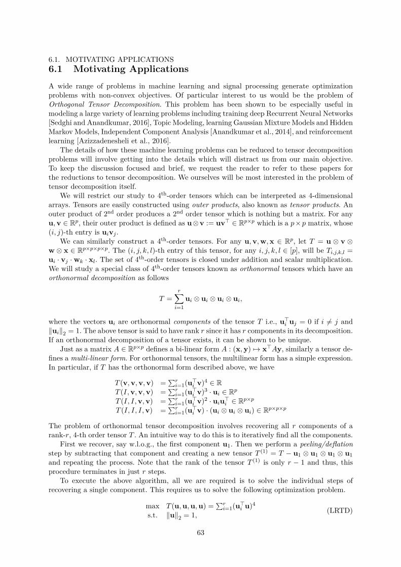
6.1. MOTIVATING APPLICATIONS6.1 Motivating ApplicationsA wide range of problems in machine learning and signal processing generate optimizationproblems with non-convex objectives. Of particular interest to us would be the problem ofOrthogonal Tensor Decomposition. This problem has been shown to be especially useful inmodeling a large variety of learning problems including training deep Recurrent Neural Networks[Sedghi and Anandkumar, 2016], Topic Modeling, learning Gaussian Mixture Models and HiddenMarkov Models, Independent Component Analysis [Anandkumar et al., 2014], and reinforcementlearning [Azizzadenesheli et al., 2016].
The details of how these machine learning problems can be reduced to tensor decompositionproblems will involve getting into the details which will distract us from our main objective.To keep the discussion focused and brief, we request the reader to refer to these papers forthe reductions to tensor decomposition. We ourselves will be most interested in the problem oftensor decomposition itself.
We will restrict our study to 4th-order tensors which can be interpreted as 4-dimensionalarrays. Tensors are easily constructed using outer products, also known as tensor products. Anouter product of 2nd order produces a 2nd order tensor which is nothing but a matrix. For anyu,v ∈ Rp, their outer product is defined as u⊗v := uv> ∈ Rp×p which is a p×p matrix, whose(i, j)-th entry is uivj .
We can similarly construct a 4th-order tensors. For any u,v,w,x ∈ Rp, let T = u ⊗ v ⊗w⊗ x ∈ Rp×p×p×p. The (i, j, k, l)-th entry of this tensor, for any i, j, k, l ∈ [p], will be Ti,j,k,l =ui · vj ·wk · xl. The set of 4th-order tensors is closed under addition and scalar multiplication.We will study a special class of 4th-order tensors known as orthonormal tensors which have anorthonormal decomposition as follows
T =r∑i=1
ui ⊗ ui ⊗ ui ⊗ ui,
where the vectors ui are orthonormal components of the tensor T i.e., u>i uj = 0 if i 6= j and‖ui‖2 = 1. The above tensor is said to have rank r since it has r components in its decomposition.If an orthonormal decomposition of a tensor exists, it can be shown to be unique.
Just as a matrix A ∈ Rp×p defines a bi-linear form A : (x,y) 7→ x>Ay, similarly a tensor de-fines a multi-linear form. For orthonormal tensors, the multilinear form has a simple expression.In particular, if T has the orthonormal form described above, we have
T (v,v,v,v) =∑ri=1(u>i v)4 ∈ R
T (I,v,v,v) =∑ri=1(u>i v)3 · ui ∈ Rp
T (I, I,v,v) =∑ri=1(u>i v)2 · uiu>i ∈ Rp×p
T (I, I, I,v) =∑ri=1(u>i v) · (ui ⊗ ui ⊗ ui) ∈ Rp×p×p
The problem of orthonormal tensor decomposition involves recovering all r components of arank-r, 4-th order tensor T . An intuitive way to do this is to iteratively find all the components.
First we recover, say w.l.o.g., the first component u1. Then we perform a peeling/deflationstep by subtracting that component and creating a new tensor T (1) = T − u1 ⊗ u1 ⊗ u1 ⊗ u1and repeating the process. Note that the rank of the tensor T (1) is only r − 1 and thus, thisprocedure terminates in just r steps.
To execute the above algorithm, all we are required is to solve the individual steps ofrecovering a single component. This requires us to solve the following optimization problem.
max T (u,u,u,u) =∑ri=1(u>i u)4
s.t. ‖u‖2 = 1, (LRTD)
63
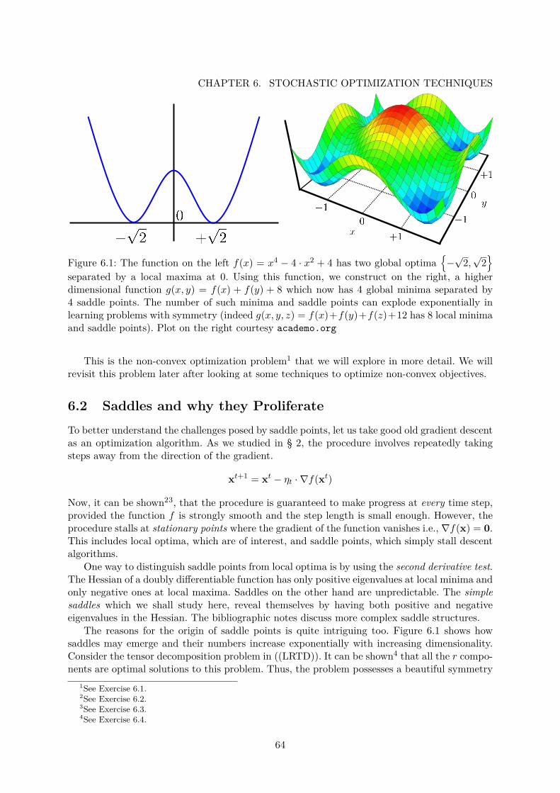
CHAPTER 6. STOCHASTIC OPTIMIZATION TECHNIQUES
Figure 6.1: The function on the left f(x) = x4 − 4 · x2 + 4 has two global optima−√
2,√
2
separated by a local maxima at 0. Using this function, we construct on the right, a higherdimensional function g(x, y) = f(x) + f(y) + 8 which now has 4 global minima separated by4 saddle points. The number of such minima and saddle points can explode exponentially inlearning problems with symmetry (indeed g(x, y, z) = f(x)+f(y)+f(z)+12 has 8 local minimaand saddle points). Plot on the right courtesy academo.org
This is the non-convex optimization problem1 that we will explore in more detail. We willrevisit this problem later after looking at some techniques to optimize non-convex objectives.
6.2 Saddles and why they Proliferate
To better understand the challenges posed by saddle points, let us take good old gradient descentas an optimization algorithm. As we studied in § 2, the procedure involves repeatedly takingsteps away from the direction of the gradient.
xt+1 = xt − ηt · ∇f(xt)
Now, it can be shown23, that the procedure is guaranteed to make progress at every time step,provided the function f is strongly smooth and the step length is small enough. However, theprocedure stalls at stationary points where the gradient of the function vanishes i.e., ∇f(x) = 0.This includes local optima, which are of interest, and saddle points, which simply stall descentalgorithms.
One way to distinguish saddle points from local optima is by using the second derivative test.The Hessian of a doubly differentiable function has only positive eigenvalues at local minima andonly negative ones at local maxima. Saddles on the other hand are unpredictable. The simplesaddles which we shall study here, reveal themselves by having both positive and negativeeigenvalues in the Hessian. The bibliographic notes discuss more complex saddle structures.
The reasons for the origin of saddle points is quite intriguing too. Figure 6.1 shows howsaddles may emerge and their numbers increase exponentially with increasing dimensionality.Consider the tensor decomposition problem in ((LRTD)). It can be shown4 that all the r compo-nents are optimal solutions to this problem. Thus, the problem possesses a beautiful symmetry
1See Exercise 6.1.2See Exercise 6.2.3See Exercise 6.3.4See Exercise 6.4.
64
6.3. THE STRICT SADDLE PROPERTYwhich allows us to recover the components in any order we like. However, it is also easy to show5
that general convex combinations of the components are not optimal solutions to this problem.Thus, we automatically obtain r isolated optima spread out in space, interspersed with saddlepoints.
The applications we discussed, such as Gaussian mixture models, also have such an internalsymmetry – the optimum is unique only up to permutation. Indeed, it does not matter in whichorder do we recover the components of a mixture model, so long as we recover all of them.However, this very symmetry gives rise to saddle points [Ge et al., 2015], since taking twopermutations of the optimal solution and taking a convex combination of them is in generalnot an optimal solution as well. This gives us, in general, an exponential number of optima,separated by (exponentially many) saddle points.
Before moving forward, we remind the reader that techniques we have studied so far fornon-convex optimization, namely EM, gAM, and gPGD are far too specific to be applied tonon-convex objectives in general, and to the problems we encounter with tensor decompositionin particular. We need more generic solutions for the task of local optimization of non-convexobjectives.
6.3 The Strict Saddle PropertyGiven that the Hessian of the function is the first point of inquiry when trying to distinguishsaddle points from other stationary points, it seems natural to use second order methods toescape points. Indeed, the bibliographic notes discuss several such approaches that use theHessian, or estimates thereof, to escape saddle points. However, these are expensive and do notscale to high dimensional problems. Consequently, we would be more interested in scalable firstorder methods.
Given the above considerations, a natural course of action is to identify properties that anobjective function should satisfy in order to allow gradient descent-style techniques to escape itssaddle points. The recent works of Ge et al. [2015], Sun et al. [2015] give an intuitive answer tothis question. They observe that if a saddle point x for a function f contains directions of steepdescent, then it is possible, at least in principle, for a gradient descent procedure to discoverthis direction and “fall” along it. The existence of such directions makes a saddle unstable –it behaves like a local maxima along these directions and a slight perturbation is very likelyto cause gradient descent to roll down the function surface. We notice that this will indeed bethe case if for some direction u ∈ Rp, we have u>∇2f(x)u 0. Figure 6.2 depicts a toy casewith the function f(x, y) = x2 − y2 which exhibits a saddle at the origin but nevertheless, alsopresents a direction of steep descent.
Consider the following unconstrained optimization problem.
minx∈Rp
f(x) (NOPT)
The following strict saddle property formalizes the requirements we have discussed in a morerobust manner.
Definition 6.1 (Strict Saddle Property [Ge et al., 2015]). A twice differentiable function f(x)is said to satisfy the (α, γ, κ, ξ)-strict saddle (SSa) property, if for every local minimum x∗ of thefunction, the function is α-strongly convex in the region B2(x∗, 2ξ) and moreover, every pointx0 ∈ Rp satisfies at least one of the following properties:
1. (Non-stationary Point) ‖∇f(x0)‖2 ≥ κ5See Exercise 6.5.
65
CHAPTER 6. STOCHASTIC OPTIMIZATION TECHNIQUES
Figure 6.2: The function f(x, y) = x2 − y2 exhibits a saddle at the origin (0, 0). The Hessian ofthis function at the origin is −2 · I and since λmin(∇2f((0, 0))) = −2, the saddle satisfies thestrict-saddle property. Indeed, the saddle does offer a prominent descent path along the y axiswhich can be used to escape the saddle point. In § 6.5 we will see how the NGD algorithm isable to provably escape this saddle point. Plot courtesy academo.org
2. (Strict Saddle Point) λmin(∇2f(x0)) ≤ −γ
3. (Approx. Local Min.) For some local minimum x∗, ‖x0 − x∗‖2 ≤ ξ.
The above property places quite a few restrictions on the function. The function mustbe strongly-convex in the neighborhood of every local optima and every point that is not anapproximate local minimum, must offer a direction of steep descent. This the point may do byhaving a steep gradient (case 1) or else (if the point is a saddle point) have its Hessian offer aneigenvector with a large negative eigenvalue which then offers a steep descent direction (case2). We shall later see that there exist interesting applications that do satisfy this property.
6.4 The Noisy Gradient Descent Algorithm
Given that the strict-saddle property assures us of the existence of a steep descent directionuntil we reach close to an approximate-local minimum, it should come as no surprise that simpletechniques should be able to achieve local optimality on functions that are strict saddle. Wewill now look at a one such simple approach to exploit the strict saddle property and achievelocal optimality.
The idea behind the approach is very simple: at every saddle point which may stall gradientdescent, the SSa property ensures that there exists a direction of steep descent. If we perturbthe gradient, there is a chance it will point in the general direction of the steep descent andescape the saddle. However, if we are at a local minimum or a non-stationary point, then thisperturbation would not affect us much.
Algorithm 6 gives the details of this approach. At each time step, it perturbs the gradientusing a unit vector pointing at a random direction in the hope that if we are currently stuck ata saddle point, the perturbation will cause us to discover the steep (enough) descent direction,allowing us to continue making progress. One easy way to obtain a random point on the unitsphere is to sample a random standard Gaussian vector w ∼ N (0, Ip×p) and normalize itζ = 1
‖w‖2·w. Notice that since the perturbation ζt is chosen uniformly from the unit sphere,
we have E[ζt]
= 0 and by linearity of expectation, E[gt |xt
]= ∇f(xt).
Such an unbiased estimate gt is often called a stochastic gradient and is widely used inmachine learning and optimization. Recall that even the EM algorithm studied in § 5 had a
66

6.5. A LOCAL CONVERGENCE GUARANTEE FOR NGDAlgorithm 6 Noisy Gradient Descent (NGD)Input: Objective f , max step length ηmax, tolerance εOutput: A locally optimal point x ∈ Rp1: x1 ← INITALIZE()2: Set T ← 1/η2, where η = min
ε2/ log2(1/ε), ηmax
3: for t = 1, 2, . . . , T do4: Sample perturbation ζt ∼ Sp−1 //Random pt. on unit sphere5: gt ← ∇f(xt) + ζt
6: xt+1 ← xt − η · gt7: end for8: return xT
variant that used stochastic gradients. In several machine learning applications, the objectivecan be written as a finite sum f(x) = 1
n
∑ni=1 f(x; θi) where θi may denote the i-th data point.
This allows us to construct a stochastic gradient estimate in an even more inexpensive manner.At each time step, simply sample a data point It ∼ Unif([n]) and let
gt = ∇f(xt,θIt) + ζt
Note that we still have E[gt |xt
]= ∇f(xt) but with a much cheaper construction for gt.
However, in order to simplify the discussion, we will continue to work with the setting gt =∇f(xt) + ζt.
We note that we have set the step lengths to be around 1/√T , where T is the total number
of iterations we are going to execute the NGD algorithm. This will seem similar to what weused in the projected gradient descent approach (see Algorithm 1 and Theorem 2.5). Althoughin practice one may set the step length to ηt ≈ 1/
√t here as well, the analysis becomes more
involved.
6.5 A Local Convergence Guarantee for NGD
We will now analyze the NGD algorithm for its convergence properties. We note that thecomplete proof requires results that are quite technical and beyond the scope of this monograph.We will instead, present the essential elements of the proof and point the curious reader to [Geet al., 2015] for the complete analysis. To simplify the notation, we will often omit specifyingthe exact constants as well.
In the following, we will assume that the function f satisfies the strict saddle property andis β-strongly smooth (see Definition 2.4). We will also assume that the function is boundedi.e., |f(x)| ≤ B for all x ∈ Rp and has ρ-Lipschitz Hessians i.e., for every x,y ∈ Rp, we have‖∇2
wf(x)−∇2wf(y)‖2 ≤ ρ ·‖x−y‖2 where ‖·‖2 for matrices denotes the spectral/operator norm
of the matrix.Before commencing with the actual proof, we first present an overview of the proof. The
definition of the SSa property clearly demarcates three different regimes:
1. Non-stationary points, i.e., points where gradient is “large” enough: in this case, standard(stochastic) gradient descent is powerful enough to ensure a large enough decrease in theobjective function value in a single step6
6See Exercise 6.2.
67
CHAPTER 6. STOCHASTIC OPTIMIZATION TECHNIQUES2. Saddle points, i.e., points where the gradient is close to 0. Here, the SSa property en-
sures that at least one highly ‘negative” Hessian direction exists: in this case, traditional(stochastic) gradient descent may fail but the additional noise ensures an escape from thesaddle point with high probability
3. Local minima, i.e., points where gradient is close to 0 but the have a positive semi definiteHessian due to strong convexity: in this case, standard (stochastic) gradient descent byitself would converge to the corresponding local minima
The above three regimes will be formally studied below in three separate lemmata. Notethat the analysis for non-stationary points as well as for points near local minima is similar tothe standard stochastic gradient descent analysis for convex functions. However, the analysisfor saddle points is quite interesting and shows that the added random noise ensures an escapefrom the saddle point.
To further understand the inner workings of the NGD algorithm, let us perform a warm-upexercise by showing that the NGD algorithm will, with high probability, escape the saddle pointin the function f(x, y) = x2 − y2 that we considered in Figure 6.2.
Theorem 6.1. Consider the function f(x, y) = x2 − y2 on two variables. If initialized atthe saddle point (0, 0) of this function with step length η < 1, with high probability, we havef(xt, yt)→ −∞ as t→∞.
Proof. For an illustration, see Figure 6.2. Note that the function f(x, y) = x2 − y2 has trivialminima at the limiting points (0,±∞) where the function value approaches −∞. Thus, thestatement of the theorem claims that NGD approaches the “minimum” function value.
In any case, we are interested in showing that NGD escapes the saddle point (0, 0). Thegradient of f is 0 at the origin (0, 0). Thus, if a gradient descent procedure is initialized at theorigin for this function, it will remain stuck there forever making no non-trivial updates.
The NGD algorithm on the other hand, when initialized at the saddle point (0, 0), aftert iterations, can be shown to reach the point (xt, yt) where xt =
∑t−1τ=0(1 − η)t−τ−1ζτ1 and
yt =∑t−1τ=0(1 + η)t−τ−1ζτ2 and (ζτ1 , ζτ2 ) ∈ R2 is the noise vector added to the gradient at each
step. Since η < 1, as t→∞, it is easy to see that with high probability, we have xt → 0 while|yt| → ∞ which indicates a successful escape from the saddle point, as well as progress towardsthe global optima.
We now formalize the intuitions developed above. The following lemma shows that even ifwe are at a saddle point, NGD will still ensure a large drop in function value in not too manysteps. The proof of this result is a bit subtle and we will just provide a sketch.
Lemma 6.2. If NGD is executed on a function f : Rp → R that is β-strongly smooth, satisfiesthe (α, γ, κ, ξ)-SSa property and has ρ-Lipschitz Hessians, with step length η ≤ 1/(β+ ρ)2, thenif an iterate xt satisfies
∥∥∇f(xt)∥∥
2 ≤√ηβ and λmin∇2f(xt) ≤ −γ, then NGD ensures that
after at most s ≤ 3 log pηγ steps,
E[f(xt+s) |xt
]≤ f(xt)− η/4
Proof. For the sake of notational simplicity, let t = 0. The overall idea of the proof is to rely onthat one large negative eigendirection in the Hessian to induce a drop in function value. Thehope is that random fluctuations will eventually nudge NGD in the steep descent direction andupon discovery, the larger and larger gradient values will accumulate to let the NGD procedureescape the saddle.
68
6.5. A LOCAL CONVERGENCE GUARANTEE FOR NGDSince the effects of the Hessian are most apparent in the second order Taylor expansion, we
will consider the following function
f(x) = f(x0) +⟨∇f(x0),x− x0
⟩+ 1
2(x− x0)>H(x− x0),
where H = ∇2f(x0) ∈ Rp×p. The proof will proceed by first imagining that NGD was executedon the function f(·) instead, showing that the function value indeed drops, and then finishing offby showing that things do not change too much if NGD is executed on the function f(·) instead.Note that to make this claim, we will need Hessians to vary smoothly which is why we assumedthe Lipschitz Hessian condition. This seems to be a requirement for several follow-up results aswell [Jin et al., 2017, Agarwal et al., 2017]. An interesting and challenging open problem is toobtain similar results for non-convex optimization without the Lipschitz-Hessian assumption.
We will let xt, t ≥ 1 denote the iterates of NGD when executed on f(·) and xt denote theiterates of NGD when executed on f(·). We will fix x0 = x0. Using some careful calculations,we can get
xt − x0 = −ηt−1∑τ=0
(I − ηH)τ∇f(x0)− ηt−1∑τ=0
(I − ηH)t−τ−1ζτ
We note that both terms in the right hand expression above correspond to “small” vectors. Thefirst term is small as we know that x0 satisfies
∥∥∇f(x0)∥∥
2 ≤√ηβ by virtue of being close to
a stationary point as is assumed in the statement of this result. The second term is small asζτ are random unit vectors with expectation 0. Using these intuitions, we will first show thatf(xt) is significantly smaller than f(x0) = f(x0) after sufficiently many steps. Then using theproperty of Lipschitz Hessians, we will obtain obtain a descent guarantee for f(xt).
Now, notice that NGD chooses the noise vectors ζτ for any τ ≥ 0, independently of x0 andH. Moreover, for any two τ 6= τ ′, the vectors ζτ , ζτ
′ are also chosen independently. We alsoknow that the noise vectors are isotropic i.e., E
[ζτ (ζτ )>
]= Ip. These observations and some
straightforward calculations give us the following upper bound on the suboptimality of xT withrespect to the Taylor approximation f . As we have noted, this upper bound can be convertedto an upper bound on the suboptimality of xT with respect to the actual function f using somemore effort.
E[f(xT )− f(x0)]
= − η∇f(x0)>t−1∑τ=0
(Ip − ηH)τ∇f(x0)
+ η2
2 ∇f(x0)>t−1∑τ=0
(Ip − ηH)τHt−1∑τ=0
(Ip − ηH)τ∇f(x0)
+ η2
2 tr(t−1∑τ=0
(Ip − ηH)2τH)
= − η∇f(x0)>B∇f(x0) + η2
2 tr(t−1∑τ=0
(Ip − ηH)2τH),
where tr(·) is the trace operator and B =∑t−1τ=0(Ip−ηH)τ− η
2∑t−1τ=0(Ip−ηH)τH
∑t−1τ=0(Ip−ηH)τ .
It is easy to verify that B 0 for all step lengths η ≤ 1‖H‖2
i.e., all η ≤ 1β .
For any value of t ≥ 3 log pηγ (which is the setting for the parameter s in the statement of the
theorem), the second term in the final expression above can be simplified to give us
η2
2 tr(t−1∑τ=0
(I − ηH)2τH)
=p∑i=1
λi(t−1∑τ=0
(1− ηλi)τ ) ≤ −η2 ,
69
CHAPTER 6. STOCHASTIC OPTIMIZATION TECHNIQUESwhere λi is the i-th eigenvalue of H, by using λp ≤ −γ. This gives us
E[f(xT )− f(x0)
]≤ −η2 .
Note that the above equation only shows descent for f(xT ). One can now show [Ge et al.,2015, Lemma 19] that the iterates obtained by NGD on f(·) do not deviate too far from thoseobtained on the actual function f(·) using the Lipschitz-Hessian property. The proof is concludedby combining these two results.
Lemma 6.3. If NGD is executed on a function that is β-strongly smooth and satisfies the(α, γ, κ, ξ)-SSa property, with step length η ≤ 1
β ·min1, κ2, then for any iterate xt that satisfies∥∥∇f(xt)
∥∥2 ≥√ηβ, NGD ensures that
E[f(xt+1) | xt
]≤ f(xt)− β
2 · η2.
Proof. This is the most carefree case as we are neither close to any local optima, nor a saddlepoint. Unsurprisingly, the proof of this lemma follows from standard arguments as we haveassumed the function to be strongly smooth. Since xt+1 = xt − η · (∇f(xt) + ζt), we have, byan application of the strong smoothness property (see Definition 2.4)
f(xt+1) ≤ f(xt)−⟨∇f(xt), η · (∇f(xt) + ζt)
⟩+ βη2
2 ·∥∥∥∇f(xt) + ζt
∥∥∥2
2.
Using the facts∥∥ζt∥∥2 = 1, E
[ζt | xt
]= 0, we get
E[f(xt+1) | xt
]≤ f(xt)− η
(1− βη
2
)∥∥∥∇f(xt)∥∥∥2
2+ βη2
2 ,
Since we have η ≤ 1β ·min
1, κ2 by assumption and
∥∥f(xt)∥∥
2 ≥√ηβ, we get
E[f(xt+1 | xt
]≤ f(xt)− β
2 · η2,
which proves the result.
The final intermediate result is an entrapment lemma. It shows that once NGD gets suf-ficiently close to a local optimum, it gets trapped there for a really long time. Although thefunction f satisfies strong convexity and smoothness properties in the neighborhood B2(x∗, 2ξ),the proof of this result is still non-trivial due to the perturbations ζt. Had the perturbations notbeen there, we could have utilized the analysis of the PGD algorithm7 to show that we wouldconverge to the local optimum x∗ at a linear rate.
The problem is that the perturbations do not diminish – we always have∥∥ζt∥∥2 = 1. This
prevents us from ever converging to the local optima. Moreover, a sequence of unfortunateperturbations may have us kicked out of this nice neighborhood. The next result shows that wewill not get kicked out of the neighborhood of x∗ for a really long time.
Lemma 6.4. If NGD is executed on a function that is β-strongly smooth and satisfies the(α, γ, κ, ξ)-SSa property, with step length η ≤ min
αβ2 , ξ
2 log−1( 1δξ )
for some δ > 0, then ifsome iterate xt satisfies
∥∥xt − x∗∥∥
2 ≤ ξ, then NGD ensures that with probability at least 1− δ,for all s ∈
[t, t+ 1
η2 log 1δ
], we have
‖xs − x∗‖2 ≤√η log 1
ηδ≤ ξ.
7See Exercise 6.3.
70
6.5. A LOCAL CONVERGENCE GUARANTEE FOR NGDProof. Using strong convexity in the neighborhood of x∗ and the fact that x∗, being a localminimum, satisfies ∇f(x∗) = 0, gives us
f(xt) ≥ f(x∗) + α
2
∥∥∥xt − x∗∥∥∥2
2
f(x∗) ≥ f(xt) +⟨∇f(xt),x∗ − xt
⟩+ α
2
∥∥∥xt − x∗∥∥∥2
2.
Together, the above two expressions give us⟨∇f(xt),xt − x∗
⟩≥ α ·
∥∥∥xt − x∗∥∥∥2
2.
Since f is β-smooth, using the co-coercivity of the gradient for smooth convex functions (recallthat f is strongly convex, in this neighborhood of x∗), we conclude that f has β-Lipschitzgradients, which gives us∥∥∥∇f(xt)
∥∥∥2
=∥∥∥∇f(xt)−∇f(x∗)
∥∥∥2≤ β ·
∥∥∥xt − x∗∥∥∥
2.
Using the above results, E[ζt | xt
]= 0 and η ≤ α
β2 gives us
E[∥∥∥xt+1 − x∗
∥∥∥2
2
∣∣∣∣ xt]
= E[∥∥∥xt − η(∇f(xt) + ζt)− x∗
∥∥∥2
2
∣∣∣∣ xt]
=∥∥∥xt − x∗
∥∥∥2
2− 2η
⟨∇f(xt),xt − x∗
⟩+ η2
∥∥∥∇f(xt)∥∥∥2
2+ η2
≤ (1− 2ηα+ η2β2) ·∥∥∥xt − x∗
∥∥∥2
2+ η2
≤ (1− ηα) ·∥∥∥xt − x∗
∥∥∥2
2+ η2,
which, upon some manipulation, gives us
E[∥∥∥xt+1 − x∗
∥∥∥2
2− η
α
∣∣∣∣ xt]≤ (1− ηα)
(∥∥∥xt − x∗∥∥∥2
2− η
α
)This tells us that on expectation, the distance of the iterates xt from the local optimum x∗ willhover around
√ηα which indicates towards the claimed result. The subsequent steps in the proof
of this result require techniques from martingale theory which we wish to avoid. We refer thereader to [Ge et al., 2015, Lemma 16] for the details.
Notice that the above result traps the iterates within a radius ξ ball around the local mini-mum x∗. Also notice that all points that are approximate local minima satisfy the preconditionsof this theorem due to the SSa property and consequently the NGD gets trapped for these points.We now present the final convergence guarantee for NGD.
Theorem 6.5. For any ε, δ > 0, suppose NGD is executed on a function that is β-stronglysmooth, has ρ-Lipschitz Hessians, and satisfies the (α, γ, κ, ξ)-SSa property, with a step lengthη < ηmax = min
ε2
log(1/εδ) ,αβ2 ,
ξ2
log(1/ξδ) ,1
(β+ρ)2 ,κ2
β
. Then, with probability at least 1 − δ, after
T ≥ log p/η2 · log(2/δ) iterations, NGD produces an iterate xT that is ε-close to some localoptimum x∗ i.e.,
∥∥∥xT − x∗∥∥∥
2≤ ε.
71
CHAPTER 6. STOCHASTIC OPTIMIZATION TECHNIQUESProof. We partition the space Rp into 3 regions
1. R1 =x : ‖f(x)‖2 ≥
√ηβ
2. R2 =x : ‖f(x)‖2 <
√ηβ, λmin(∇2f(x)) ≤ −γ
3. R3 = Rp\(R1 ∪R2)
Since√ηβ ≤ κ due to the setting of ηmax, the region R1 contains all points considered non-
stationary by the SSa property (Definition 6.1) and possibly some other points as well. For thisreason, region R2 can be shown to contain only saddle points. Since the SSa property assuresus that a point that is neither non-stationary nor a saddle point is definitely an approximatelocal minimum, we deduce that the region R3 contains only approximately local minima.
The proof will use the following line of argument: since Lemmata 6.3 and 6.2 assure us thatwhenever the NGD procedure is in regions R1 or R2 there is a large drop in function value, weshould expect the procedure to enter region R3 sooner or later, since the function value cannotgo on decreasing indefinitely. However, Lemma 6.4 shows that once we are in region R3, weare trapped there. In the following analysis, we will ignore all non-essential constants and logfactors.
Recall that we let the NGD procedure last for T = 1/η2 log(2/δ) steps. Below we will showthat in any sequence of 1/η2 steps, there is at least a 1/2 chance of encountering an iteratext ∈ R3. Since the entire procedure lasts log(1/δ) such sequences, we will conclude, by unionbound, that with probability at least 1−δ/2, we will encounter at least one iterate in the regionR3 in the T steps we execute.
However, Lemma 6.4 shows that once we enter the R3 neighborhood, with probability atleast 1− δ/2, we are trapped there for at least T steps. Applying the union bound will establishthat with probability at least 1 − δ, the NGD procedure will output xT ∈ R3. Since we setη ≤ ε2/ log(1/εδ), this will conclude the proof.
We now left with proving that in every sequence of 1/η2 steps, there is at least a 1/2 chanceof NGD encountering an iterate xt ∈ R3. To do so, we set up the notion of epochs. These willbasically correspond to the amount of time taken by NGD to reduce the function value by asignificant amount. The first epoch starts at time τ1 = 0. Subsequently, we define
τi+1 =τi + 1 if xτi ∈ R1 ∪R3τi + 1
η if xτi ∈ R2
Ignoring constants and other non-essential factors, we can rewrite the results of Lemmata 6.3and 6.2 as follows
E [f(xτi+1)− f(xτi) | xτi ∈ R1] ≤ −η2
E [f(xτi+1)− f(xτi) | xτi ∈ R2] ≤ −η
Putting these together gives us
E [f(xτi+1)− f(xτi) | xτi /∈ R3] ≤ −E [(τi+1 − τi) | xτi /∈ R3] · η2
Define the event Et :=@ j ≤ t : xj ∈ R3
and let 1E denote the indicator variable for event E
i.e., 1E = 1 if E occurs and 1E = 0 otherwise. Then we have
E[f(xτi+1) · 1Eτi+1
− f(xτi) · 1Eτi
]= E
[f(xτi+1) · (1Eτi+1
− 1Eτi)]
+ E[(f(xτi+1)− f(xτi)) · 1Eτi
]≤ B · (P
[Eτi+1
]− P [Eτi ])− η2 · E
[τi+1 − τi | 1Eτi
]· P [Eτi ] ,
72
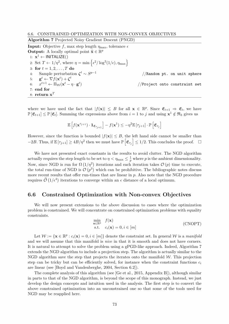
6.6. CONSTRAINED OPTIMIZATION WITH NON-CONVEX OBJECTIVESAlgorithm 7 Projected Noisy Gradient Descent (PNGD)Input: Objective f , max step length ηmax, tolerance εOutput: A locally optimal point x ∈ Rp1: x1 ← INITALIZE()2: Set T ← 1/η2, where η = min
ε2/ log2(1/ε), ηmax
3: for t = 1, 2, . . . , T do4: Sample perturbation ζt ∼ Sp−1 //Random pt. on unit sphere5: gt ← ∇f(xt) + ζt
6: xt+1 ← ΠW(xt − η · gt) //Project onto constraint set7: end for8: return xT
where we have used the fact that |f(x)| ≤ B for all x ∈ Rp. Since Et+1 ⇒ Et, we haveP [Et+1] ≤ P [Et]. Summing the expressions above from i = 1 to j and using x1 /∈ R3 gives us
E[f(xτj+1) · 1Eτj+1
]− f(x1) ≤ −η2E [τj+1] · P
[Eτj
]However, since the function is bounded |f(x)| ≤ B, the left hand side cannot be smaller than−2B. Thus, if E [τj+1] ≥ 4B/η2 then we must have P
[Eτj
]≤ 1/2. This concludes the proof.
We have not presented exact constants in the results to avoid clutter. The NGD algorithmactually requires the step length to be set to η < ηmax ≤ 1
p where p is the ambient dimensionality.Now, since NGD is run for Ω
(1/η2) iterations and each iteration takes O (p) time to execute,
the total run-time of NGD is O(p3) which can be prohibitive. The bibliographic notes discuss
more recent results that offer run-times that are linear in p. Also note that the NGD procedurerequires O
(1/ε4
)iterations to converge within an ε distance of a local optimum.
6.6 Constrained Optimization with Non-convex Objectives
We will now present extensions to the above discussion to cases where the optimizationproblem is constrained. We will concentrate on constrained optimization problems with equalityconstraints.
minx∈Rp
f(x)s.t. ci(x) = 0, i ∈ [m]
(CNOPT)
LetW := x ∈ Rp : ci(x) = 0, i ∈ [m] denote the constraint set. In generalW is a manifoldand we will assume that this manifold is nice in that it is smooth and does not have corners.It is natural to attempt to solve the problem using a gPGD-like approach. Indeed, Algorithm 7extends the NGD algorithm to include a projection step. The algorithm is actually similar to theNGD algorithm save the step that projects the iterates onto the manifold W. This projectionstep can be tricky but can be efficiently solved, for instance when the constraint functions ciare linear (see [Boyd and Vandenberghe, 2004, Section 6.2]).
The complete analysis of this algorithm (see [Ge et al., 2015, Appendix B]), although similarin parts to that of the NGD algorithm, is beyond the scope of this monograph. Instead, we justdevelop the design concepts and intuition used in the analysis. The first step is to convert theabove constrained optimization into an unconstrained one so that some of the tools used forNGD may be reapplied here.
73
CHAPTER 6. STOCHASTIC OPTIMIZATION TECHNIQUESA very common way to do so is to first construct the Lagrangian [Boyd and Vandenberghe,
2004, Chapter 5] of the problem defined as
L(x,λ) = f(x)−m∑i=1
λici(x),
where λi are Lagrange multipliers. It is easy to verify that the solution to the problem((CNOPT)) coincides with that of the following problem
minx∈Rp
maxλ∈Rm
L(x,λ)
Note that the above problem is unconstrained. For any x ∈ Rp, define λ∗(x) :=arg minλ ‖∇f(x)−
∑mi=1 λi∇ci(x)‖ and L∗(x) := L(x,λ∗(x)). We also define the tangent and
normal spaces of the manifold W as follows.Definition 6.2 (Normal and Tangent Space). For a manifold W defined as the intersectionof m constraints of the form ci(x) = 0, given any x ∈ W, define its tangent space as T (x) =v | 〈∇ci(x),v〉 = 0, i ∈ [m] and its normal space as T c(x) = span ∇c1(x), . . . ,∇cm(x).
If we think ofW as a smooth surface, then at any point, the tangent space defines the tangentplane of the surface at that point and the normal space consists of all vectors orthogonal tothe tangent plane. The reason behind defining all the above quantities is the following. Inunconstrained optimization we have the first and second order optimality conditions: if x∗ is alocal minimum for f(·) then ∇f(x∗) = 0 and ∇2f(x∗) 0.
Along the same lines, for constrained optimization problems, similar conditions exist char-acterizing stationary and optimal points: one can show [Wright and Nocedal, 1999] that if x∗is a local optimum for the constrained problem ((CNOPT)), then we must have ∇L∗(x∗) = 0,as well as v>∇2L∗(x∗)v ≥ 0 for all v ∈ T (x∗). This motivates us to propose the followingextension of the strict saddle property for constrained optimization problems.Definition 6.3 (Strict Constrained Saddle Property [Ge et al., 2015]). A twice differentiablefunction f(x) with a constraint set W is said to satisfy the (α, γ, κ, ξ)-strict constrained saddle(SCSa) property, if for every local minimum x∗ ∈ W, we have v>L∗(x′)v ≥ α for all v ∈T (x′), ‖v‖2 = 1 and for all x′ in the region B2(x∗, 2ξ), and moreover, any point x0 ∈ Rpsatisfies at least one of the following properties:
1. (Non-Stationary) ‖∇L∗(x0)‖2 ≥ κ
2. (Strict Saddle) v>∇2L∗(x0)v ≤ −γ for some v ∈ T (x0), ‖v‖2 = 1
3. (Approx. Local Min.) For some local minimum x∗, ‖x0 − x∗‖2 ≤ ξ.The following local convergence result can then be shown for the PNGD algorithm.
Theorem 6.6. Suppose PNGD is executed on a constrained optimization problem that satisfiesthe (α, γ, κ, ξ)-SCSa property, has ρ-Lipschitz Hessians and whose constraint set is a smoothmanifold W. Then there exists a constant ηmax = Θ(1) such that for any ε, δ > 0, if we set η =min
ηmax,
ε2
log(1/εδ)
, then with probability at least 1− δ, after T ≥ log p/η2 · log(2/δ) iterations,
PNGD produces an iterate xT that is ε-close to some local optimum x∗ i.e.,∥∥∥xT − x∗
∥∥∥2≤ ε.
The PNGD procedure requires O(1/ε4
)iterations to converge within an ε distance of a local
optimum, similar to NGD. The proof of the above theorem [Ge et al., 2015, Lemma 35] proceedsby showing that the PNGD updates can be rewritten as
xt+1 = xt − η · (∇L∗(xt) + ΠT (xt)(ζt)) + ιt,
where ΠT (xt)(·) is the projection of a vector onto the tangent space T (xt) and ιt is an errorvector with small norm
∥∥ιt∥∥2 ≤ η2.
74

6.7. APPLICATION TO ORTHOGONAL TENSOR DECOMPOSITION6.7 Application to Orthogonal Tensor Decomposition
Recall that we reduced the tensor decomposition problem to solving the following optimizationproblem ((LRTD))
max T (u,u,u,u) =∑ri=1(u>i u)4
s.t. ‖u‖2 = 1,
The above problem has internal symmetry with respect to permutation of the components, aswell as sign flips (both ui and −ui are valid components) which gives rise to saddle points aswe discussed earlier. Using some simple but slightly tedious calculations (see [Ge et al., 2015,Theorem 44, Lemmata 45, 46]) it is possible to show that the above optimization problem doessatisfy the (3, 7/p, 1/pc, 1/pc)-SCSa property for some constant c > 0. All other requirementsfor Theorem 6.6 can also be shown to be satisfied.
It is easy to see that any solution to the problem must lie in the span of the components.Since the components ui are orthonormal, this means that it suffices to look for solutionsof the form u =
∑ri=1 xiui. This gives us T (u,u,u,u) =
∑ri=1 x
4i , and ‖u‖2 = ‖x‖2 where
x = [x1, x2, . . . , xr]. This allows us to formulate the equivalent problem as
min −‖x‖44s.t. ‖x‖2 = 1,
Note that the above problem is non-convex as the objective function is concave. However, it isalso possible to show89 that the only local minima of the optimization problem ((LRTD)) are±ui. This is most fortunate since it shows that all local minima are actually global minima! Thus,the deflation strategy alluded to earlier can be successfully applied. We discover one component,say u1 by applying the PNGD algorithm to ((LRTD)). Having recovered this component, wecreate a new tensor T ′ = T −u1⊗u1⊗u1⊗u1, apply the procedure again to discover a secondcomponent and so on.
The work of Ge et al. [2015] also discusses techniques to recover all r components simulta-neously, tensors with different positive weights on the components, as well as tensors of otherorders.
6.8 Exercises
Exercise 6.1. Show that the optimization problem in the formulation ((LRTD)) is non-convexin that it has a non-convex objective as well as a non-convex constraint set. Show that constraintset may be convexified without changing the optimum of the problem.
Exercise 6.2. Consider a differentiable function f that is β-strongly smooth but possibly non-convex. Show that if gradient descent is performed on f with a static step length η ≤ 2
β i.e.,
xt+1 = xt − η · ∇f(xt)
then the function value f will never increase across iterations i.e., f(xt+1) ≤ f(xt). This showsthat on smooth functions, gradient descent enjoys monotonic progress whenever the step lengthis small enough.Hint: apply the SS property relating consecutive iterates.
8See Exercise 6.4.9See Exercise 6.5.
75
CHAPTER 6. STOCHASTIC OPTIMIZATION TECHNIQUESExercise 6.3. For the same setting as the previous problem, show that if we have η ∈
[1
2β ,1β
]instead, then within T = O
(1ε2
)steps, gradient descent is guaranteed to identify an ε-stationary
point i.e for some t ≤ T , we must have∥∥∇f(xt)
∥∥2 ≤ ε.
Hint: first apply SS to show that f(xt) − f(xt+1) ≥ 14β ·
∥∥∇f(xt)∥∥2
2. Then use the fact that thetotal improvement in function value over T time steps cannot exceed f(x0)− f∗.
Exercise 6.4. Show that every component vector ui is a globally optimal point for the opti-mization problem in ((LRTD)).Hint: Observe the reduction in § 6.7. Show that it is equivalent to finding the minimum L2 normvector(s) among unit L1 norm vectors. Find the Lagrangian dual of this optimization problemand simplify.
Exercise 6.5. Given a rank-r orthonormal tensor T , construct a non-trivial convex combina-tion of its components that has unit L2 norm but achieves a suboptimal objective value in theformulation ((LRTD)).
6.9 Bibliographic NotesProgress in this area was extremely rapid at the time of writing this monograph. The followingdiscussion outlines some recent advances.
The general problem of local optimization has been of interest in the optimization communityfor several years. Some of the earlier results in the area concentrated on second order or quasi-Newton methods, understandably since the Hessians can be used to distinguish between localoptima and saddle points. Some key works include those of Nesterov and Polyak [2006], Dauphinet al. [2014], Sun et al. [2015], Yuan [2015]. However, these techniques can be expensive andhence, are not used in high dimensional applications.
Algorithms for specialized applications, such as the EM algorithm we studied in § 5, havereceived independent attention with respect to their local convergence properties. We referthe reader to the bibliographic notes § 5.11 for the same. In recent years, the problem ofoptimization of general non-convex problems has been looked at from several perspectives.Below we outline some of the major thrust areas.
First Order Methods Given their efficiency, the question of whether first order methods canoffer local optimality has captured the interest of the field. In particular, much attention hasbeen paid to the standard gradient descent and its variants. The work of Lee et al. [2016] showedthat when initialized at a random point, gradient descent avoids saddle points almost surely,although the work provides no definite rate of convergence in general.
The subsequent works of Sun et al. [2015], Ge et al. [2015], Anandkumar and Ge [2016]introduced structural properties such as the strict saddle property, and demonstrated that crispconvergence rates can be ensured for problems that do satisfy these structural properties. It isnotable that the work of Sun et al. [2015] reconsidered second order methods while Ge et al.[2015] were able to show that noisy stochastic gradient descent itself suffices.
The technique of using randomly perturbed (stochastic) gradients to escape saddle pointsreceives attention in a more general framework of Langevin Dynamics which study cases whenthe perturbations are non-isotropic or else are applied at a scale that adapts to the problem.The recent work of Zhang et al. [2017] shows a powerful result that offers, for empirical riskminimization problems that are ubiquitous in machine learning, a convergence guarantee thatensures convergence to a local optimum of the population risk functional. This is a useful resultsince a majority of works in literature focus on identifying local optima of the empirical risk
76
6.9. BIBLIOGRAPHIC NOTESfunctional, which depend on the training data, but which may correspond to bad solutionswith respect to the population risk.
Non-smooth Optimization All techniques we discussed in thus far in this monographrequire the objective function to at least be differentiable. In fact, we go one step ahead toassume (restricted) smoothness. The work of Reddi et al. [2016] shows how variance reductiontechniques may be exploited to ensure ε-convergence to a first-order stationary point xt(effectively a saddle point) where we have
∥∥f(xt)∥∥
2 ≤ ε, in no more than O (1/ε) iterationsof stochastic mini-batch gradient descent even when the objective function is non-convex andnon-smooth at the same time. We urge the reader to confer this with Exercise 6.3 where it tookO(1/ε2
)iterations to do the same, that too using full gradient descent. Also notable is the fact
that in our analysis (see Theorem 6.5), it took NGD O(1/ε4
)steps to reach a local optimum.
However, two caveats exist: 1) the method proposed in [Reddi et al., 2016] only reaches asaddle point, and 2) it assumes a finite-sum objective, i.e., one that has a decomposable form.
Accelerated Optimization The works of Carmon et al. [2017], Agarwal et al. [2017] extendthe work of Reddi et al. [2016] by offering faster than O
(1/ε2
)convergence to a stationary
point for general (non finite-sum) non-convex objectives. However, it should be noted that thesetechniques assume a smooth objective and convergence is guaranteed only to a saddle point, nota local minimum. Whereas the work of Carmon et al. [2017] invokes a variant of Nesterov’s ac-celerated gradient technique to offer ε-convergence in O
(1/ε7/4
)iterations, the work of Agarwal
et al. [2017] employs a second-order method to offer ε-convergence, also in O(1/ε7/4
)iterations.
High-dimensional Optimization When considering problems in high-dimensions, it be-comes difficult to execute algorithms whose run-times scale super-linearly in the ambientdimensionality. This is one reason why first-order methods are preferred. However, as we saw,the overall run-time of Theorem 6.5 scales as O
(p3) which makes the method prohibitive even
for moderate dimensional problems. The work of Jin et al. [2017] proposes another perturbedgradient method that offers a run-time that depends only quasi-linearly on the ambientdimension. It should be noted that the works of Carmon et al. [2017], Agarwal et al. [2017]also offer run-times that are linear in the ambient dimensionality although, as noted earlier,convergence is only guaranteed to a saddle point by these methods.
Escaping Higher-order Saddles In our discussion, we were occupied with the problemof avoiding getting stuck at simple saddle points which readily reveal themselves by havingdistinctly positive and negative eigenvalues in the Hessian. However, there may exist morecomplex degenerate saddle points where the Hessian has only non-negative eigenvalues andthus, masquerades as a local minima. Such configurations yield complex cases such as monkeysaddles and connected saddles. We did not address these. The work of Anandkumar andGe [2016] proposes a method based on the Cubic Regularization algorithm of Nesterov andPolyak [2006] which is able to escape some of these more complex saddle points and achieveconvergence to a point that enjoys third order optimality.
Training Deep Networks Given the popularity of deep networks in several areas of learningand signal processing, as well as the fact that the task of training deep networks correspondsto non-convex optimization, a lot of recent efforts have focused on the problem of efficientlyand provably training deep networks using non-convex optimization techniques. Some notableworks include provable methods for training multi-layered perceptrons [Goel and Klivans, 2017,Zhong et al., 2017, Li and Yuan, 2017] and special cases of convoluational networks known as
77

CHAPTER 6. STOCHASTIC OPTIMIZATION TECHNIQUESnon-overlapping convolutional networks [Brutzkus and Globerson, 2017]. Whereas the works[Brutzkus and Globerson, 2017, Zhong et al., 2017, Li and Yuan, 2017] utilize gradient-descentbased techniques, Goel and Klivans [2017] uses an application of isotonic regression and kerneltechniques. The work of Li and Yuan [2017] shows that the inclusion of an identity map intothe network eases optimization by making the training problem well-posed.
78

The official publication is available from now publishers viahttp://dx.doi.org/10.1561/2200000058
Part III
Applications
79
The official publication is available from now publishers viahttp://dx.doi.org/10.1561/2200000058
Chapter 7
Sparse Recovery
In this section, we will take a look at the sparse recovery and sparse linear regression as ap-plications of non-convex optimization. These are extremely well studied problems and findapplications in several practical settings. This will be the first of four “application” sectionswhere we apply non-convex optimization techniques to real-world problems.
7.1 Motivating Applications
We will take the following two running examples to motivate the sparse regression problem intwo different settings.
Gene Expression Analysis The availability of DNA micro-array gene expression data makesit possible to identify genetic explanations for a wide range of phenotypical traits such asphysiological properties or even disease progressions. In such data, we are given say, for nhuman test subjects participating in the study, the expression levels of a large number p ofgenes (encoded as a real vector xi ∈ Rp), and the corresponding phenotypical trait yi ∈ R.Figure 7.1 depicts this for a hypothetical study on Type-I diabetes. For the sake of simplicity,we are considering cases where the phenotypical trait can be modeled as a real number –this real number may indicate the severity of a condition or the level of some other biologicalmeasurement. More expressive models exist in literature where the target phenotypical trait isitself represented as a vector [see for example, Jain and Tewari, 2015].
For the sake of simplicity, we assume that the phenotypical response is linearly linked tothe gene expression levels i.e. for some w∗ ∈ Rp, we have yi = x>i w∗ + ηi where ηi is somenoise. The goal then is to use gene expression data to deduce an estimate for w∗. Having accessto the model w∗ can be instrumental in discovering possible genetic bases for diseases, traitsetc. Consequently, this problem has significant implications for understanding physiology anddeveloping novel medical interventions to treat and prevent diseases/conditions.
However, the problem fails to reduce to a simple linear regression problem for two importantreasons. Firstly, although the number of genes whose expression levels are being recordedis usually very large (running into several tens of thousands), the number of samples (testsubjects) is usually not nearly as large, i.e. n p. Traditional regression algorithms fall silentin such data-starved settings as they usually expect n > p. Secondly, and more importantly,we do not expect all genes being tracked to participate in realizing the phenotype. Indeed,the whole objective of this exercise is to identify a small set of genes which most prominentlyinfluence the given phenotype. Note that this implies that the vector w∗ is very sparse.Traditional linear regression cannot guarantee the recovery of a sparse model.
80
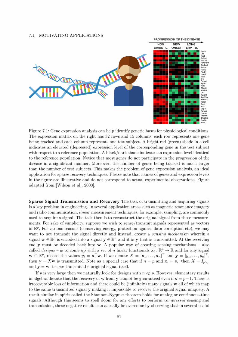
7.1. MOTIVATING APPLICATIONSPROGRESSION OF THE DISEASE
Gpx3Lp1Tcp1Eef1a1S1c126MMU474Atp5a3AcatnHipk2Pkd2Hao3Scd1ErdFkbp4Rp121ActbCCnd1Nfe212Cf11Rps23Rp137aNdufa7Rp1p1Oaz1Sod1VapaPsmb1Cd24aTacstdlZfp3611Cox7bIDH1
NON DIABETIC
NEW ONSET
LONG TERM T1D
Figure 7.1: Gene expression analysis can help identify genetic bases for physiological conditions.The expression matrix on the right has 32 rows and 15 columns: each row represents one genebeing tracked and each column represents one test subject. A bright red (green) shade in a cellindicates an elevated (depressed) expression level of the corresponding gene in the test subjectwith respect to a reference population. A black/dark shade indicates an expression level identicalto the reference population. Notice that most genes do not participate in the progression of thedisease in a significant manner. Moreover, the number of genes being tracked is much largerthan the number of test subjects. This makes the problem of gene expression analysis, an idealapplication for sparse recovery techniques. Please note that names of genes and expression levelsin the figure are illustrative and do not correspond to actual experimental observations. Figureadapted from [Wilson et al., 2003].
Sparse Signal Transmission and Recovery The task of transmitting and acquiring signalsis a key problem in engineering. In several application areas such as magnetic resonance imageryand radio communication, linear measurement techniques, for example, sampling, are commonlyused to acquire a signal. The task then is to reconstruct the original signal from these measure-ments. For sake of simplicity, suppose we wish to sense/transmit signals represented as vectorsin Rp. For various reasons (conserving energy, protection against data corruption etc), we maywant to not transmit the signal directly and instead, create a sensing mechanism wherein asignal w ∈ Rp is encoded into a signal y ∈ Rn and it is y that is transmitted. At the receivingend y must be decoded back into w. A popular way of creating sensing mechanisms – alsocalled designs – is to come up with a set of n linear functionals xi : Rp → R and for any signalw ∈ Rp, record the values yi = x>i w. If we denote X = [x1, . . . ,xn]> and y = [y1, . . . , yn]>,then y = Xw is transmitted. Note as a special case that if n = p and xi = ei, then X = Ip×pand y = w, i.e. we transmit the original signal itself.
If p is very large then we naturally look for designs with n p. However, elementary resultsin algebra dictate that the recovery of w from y cannot be guaranteed even if n = p−1. There isirrecoverable loss of information and there could be (infinitely) many signals w all of which mapto the same transmitted signal y making it impossible to recover the original signal uniquely. Aresult similar in spirit called the Shannon-Nyquist theorem holds for analog or continuous-timesignals. Although this seems to spell doom for any efforts to perform compressed sensing andtransmission, these negative results can actually be overcome by observing that in several useful
81
CHAPTER 7. SPARSE RECOVERYsettings, the signals we are interested in, are actually very sparse i.e. w ∈ B0(s) ⊂ Rp, s p.This realization is critical since it allows the possibility of specialized design matrices to be usedto transmit sparse signals in a highly compressed manner i.e. with n p but without any lossof information. However the recovery problem now requires a sparse vector to be recovered fromthe transmitted signal y and the design matrix X.
7.2 Problem Formulation
In both the examples considered above, we wish to recover a sparse linear model w ∈ B0(s) ⊂ Rpthat fits the data, i.e., yi ≈ x>i w, hence the name sparse recovery. In the gene analysis problem,the support of such a model w is valuable in revealing the identity of the genes involved inpromoting the given phenotype/disease. Similarly, in the sparse signal recovery problem, w isthe (sparse) signal itself.
This motivates the sparse linear regression problem. In the following, we shall use xi ∈ Rp todenote the features (gene expression levels/measurement functionals). Each feature will consti-tute a data point. There will be a response variable yi ∈ R (phenotype response/measurement)associated with each data point. We will assume that the response variables are being gener-ated using some underlying sparse model w∗ ∈ B0(s) (gene influence pattern/sparse signal) asyi = x>i w∗ + ηi where ηi is some benign noise.
In both the gene expression analysis problem, as well as the sparse signal recovery prob-lem, recovering w∗ from the data (x1, y1), . . . , (xn, yn) then requires us to solve the followingoptimization problem: min
w∈Rp,‖w‖0≤s
∑ni=1
(yi − x>i w
)2. Rewriting the above in more succinct
notation gives usmin
w∈Rp‖w‖0≤s
‖y−Xw‖22 , (SP-REG)
where X = [x1, . . . ,xn]> and y = [y1, . . . , yn]>. It is common to model the additive noise aswhite noise i.e. ηi ∼ N (0, σ2) for some σ > 0. It should be noted that the sparse regressionproblem in ((SP-REG)) is an NP-hard problem [Natarajan, 1995].
7.3 Sparse Regression: Two Perspectives
Although we cast both the gene analysis and sparse signal recovery problems in the sameframework of sparse linear regression, there are subtle but crucial differences between the twoproblem settings.
Notice that the problem in sparse signal recovery is to come up with both, a design matrixX, as well as a recovery algorithm A : Rn × Rn×p → Rp such that all sparse signals can beaccurately recovered from the measurements, i.e. ∀w ∈ B0(s) ⊂ Rp, we have A(Xw, X) ≈ w.
On the other hand, in the gene expression analysis task, we do not have as direct a controlover the effective design matrix X. In this case, the role of the design matrix is played by thegene expression data of the n test subjects. Although we may choose which individuals we wishto include in our study, even this choice does not give us a direct handle on the properties of thedesign matrix. Our job here is restricted to coming up with an algorithm A which can, giventhe gene expression data for p genes in n test subjects, figure out a sparse set of s genes whichcollectively promote the given phenotype i.e. for any w ∈ B0(s) ⊂ Rp and given X ∈ Rn×p, wedesire A(Xw, X) ≈ w.
The distinction between the two settings is now apparent: in the first setting, the designmatrix is totally in our control. We may design it to have specific properties as required by the
82
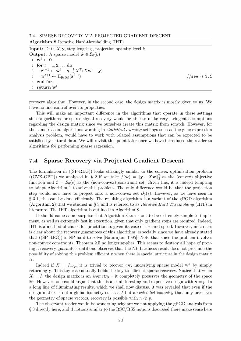
7.4. SPARSE RECOVERY VIA PROJECTED GRADIENT DESCENTAlgorithm 8 Iterative Hard-thresholding (IHT)Input: Data X,y, step length η, projection sparsity level kOutput: A sparse model w ∈ B0(k)1: w1 ← 02: for t = 1, 2, . . . do3: zt+1 ← wt − η · 1
nX>(Xwt − y)
4: wt+1 ← ΠB0(k)(zt+1) //see § 3.15: end for6: return wt
recovery algorithm. However, in the second case, the design matrix is mostly given to us. Wehave no fine control over its properties.
This will make an important difference in the algorithms that operate in these settingssince algorithms for sparse signal recovery would be able to make very stringent assumptionsregarding the design matrix since we ourselves create this matrix from scratch. However, forthe same reason, algorithms working in statistical learning settings such as the gene expressionanalysis problem, would have to work with relaxed assumptions that can be expected to besatisfied by natural data. We will revisit this point later once we have introduced the reader toalgorithms for performing sparse regression.
7.4 Sparse Recovery via Projected Gradient Descent
The formulation in ((SP-REG)) looks strikingly similar to the convex optimization problem((CVX-OPT)) we analyzed in § 2 if we take f(w) = ‖y−Xw‖22 as the (convex) objectivefunction and C = B0(s) as the (non-convex) constraint set. Given this, it is indeed temptingto adapt Algorithm 1 to solve this problem. The only difference would be that the projectionstep would now have to project onto a non-convex set B0(s). However, as we have seen in§ 3.1, this can be done efficiently. The resulting algorithm is a variant of the gPGD algorithm(Algorithm 2) that we studied in § 3 and is referred to as Iterative Hard Thresholding (IHT) inliterature. The IHT algorithm is outlined in Algorithm 8.
It should come as no surprise that Algorithm 8 turns out to be extremely simple to imple-ment, as well as extremely fast in execution, given that only gradient steps are required. Indeed,IHT is a method of choice for practitioners given its ease of use and speed. However, much lessis clear about the recovery guarantees of this algorithm, especially since we have already statedthat ((SP-REG)) is NP-hard to solve [Natarajan, 1995]. Note that since the problem involvesnon-convex constraints, Theorem 2.5 no longer applies. This seems to destroy all hope of prov-ing a recovery guarantee, until one observes that the NP-hardness result does not preclude thepossibility of solving this problem efficiently when there is special structure in the design matrixX.
Indeed if X = Ip×p, it is trivial to recover any underlying sparse model w∗ by simplyreturning y. This toy case actually holds the key to efficient sparse recovery. Notice that whenX = I, the design matrix is an isometry – it completely preserves the geometry of the spaceRp. However, one could argue that this is an uninteresting and expensive design with n = p. Ina long line of illuminating results, which we shall now discuss, it was revealed that even if thedesign matrix is not a global isometry such as I but a restricted isometry that only preservesthe geometry of sparse vectors, recovery is possible with n p.
The observant reader would be wondering why are we not applying the gPGD analysis from§ 3 directly here, and if notions similar to the RSC/RSS notions discussed there make sense here
83

CHAPTER 7. SPARSE RECOVERYtoo. We request the reader to read on. We will find that not only do those notions extend here,but have beautiful interpretations. Moreover, instead of directly applying the gPGD analysis(Theorem 3.3), we will see a simpler convergence proof tailored to the sparse recovery problemwhich also gives a sharper result.
7.5 Restricted Isometry and Other Design Properties
As we observed previously, design matrices such as Ip which preserve the geometry of sig-nals/models seem to allow for recovery of sparse signals. We now formalize this intuition furtherand develop specific conditions on the design matrix X which guarantee universal recovery i.e.for every w ∈ B0(s), it is possible to uniquely recover w from the measurements Xw.
It is easy to see that a design matrix that identifies sparse vectors cannot guarantee universalrecovery. Suppose we have a design matrix X ∈ Rn×p such that for some w1,w2 ∈ B0(s) andw1 6= w2, we get y1 = y2 where y1 = Xw1 and y2 = Xw2. In this case, it is informationtheoretically impossible to distinguish between w1 and w2 on the basis of measurements madeusing X i.e. using y1 (or y2). Consequently, this design matrix cannot be used for universalrecovery since it produces measurements that confuse between sparse vectors. It can be seen1that such a design matrix will not identify just one pair of sparse vectors but an infinite set ofpairs (indeed an entire subspace) of sparse vectors.
Thus, it is clear that the design matrix must preserve the geometry of the set of sparse vectorswhile projecting them from a high p-dimensional space to a low n-dimensional space. Recall thatin sparse recovery settings, we usually have n p. The Nullspace Property presented below, andthe others thereafter, are formalizations of this intuition. For any subset of coordinates S ⊂ [p],let us define the set C(S) :=
w ∈ Rp, ‖wS‖1 ≥
∥∥wS
∥∥1
. This is the (convex) set of points that
place a majority of their weight on coordinates in the set S. Define C(k) :=⋃S:|S|=k C(S) to
be the (non-convex2) set of points that place a majority of their weight on some k coordinates.Note that C(k) ⊃ B0(k) since k-sparse vectors put all their weight on some k coordinates.
Definition 7.1 (Nullspace Property [Cohen et al., 2009]). A matrix X ∈ Rn×p is said to satisfythe null-space property of order k if ker(X) ∩ C(k) = 0, where ker(X) = w ∈ Rp : Xw = 0is the kernel of the linear transformation induced by X (also called its null-space).
If a design matrix satisfies this property, then vectors in its null-space are disallowed fromconcentrating a majority of their weight on any k coordinates. Clearly no k-sparse vector ispresent in the null-space either. If a design matrix has the null-space property of order 2s, thenit can never identify two s-sparse vectors3 – something that we have already seen as essentialto ensure global recovery. A strengthening of the Nullspace Property gives us the RestrictedEigenvalue Property.
Definition 7.2 (Restricted Eigenvalue Property [Raskutti et al., 2010]). A matrix X ∈ Rn×p issaid to satisfy the restricted eigenvalue property of order k with constant α if for all w ∈ C(k),we have 1
n ‖Xw‖22 ≥ α · ‖w‖22.
This means that not only are k-sparse vectors absent from the null-space, they actuallyretain a good fraction of their length after projection as well. This means that if k = 2s, thenfor any w1,w2 ∈ B0(s), we have 1
n ‖X(w1 −w2)‖22 ≥ α·‖w1 −w2‖22. Thus, the distance betweenany two sparse vectors never greatly diminished after projection. Such behavior is the hallmark
1See Exercise 7.1.2See Exercise 7.2.3See Exercise 7.3.
84
7.6. ENSURING RIP AND OTHER PROPERTIESof an isometry, which preserves the geometry of vectors. The next property further explicatesthis and is, not surprisingly, called the Restricted Isometry Property.
Definition 7.3 (Restricted Isometry Property [Candès and Tao, 2005]). A matrix X ∈ Rn×pis said to satisfy the restricted isometry property (RIP) of order k with constant δk ∈ [0, 1) iffor all w ∈ B0(k), we have
(1− δk) · ‖w‖22 ≤1n ‖Xw‖22 ≤ (1 + δk) · ‖w‖22.
The above property is most widely used in analyzing sparse recovery and compressive sensingalgorithms. However, it is a bit restrictive since it requires the distortion parameters to be ofthe kind (1 ± δ) for δ ∈ [0, 1). A generalization of this property that is especially useful insettings where the properties of the design matrix are not strictly controlled by us, such asthe gene expression analysis problem, is the following notion of restricted strong convexity andsmoothness.
Definition 7.4 (Restricted Strong Convexity/Smoothness Property [Jain et al., 2014, Jalaliet al., 2011]). A matrix X ∈ Rn×p is said to satisfy the α-restricted strong convexity (RSC)property and the β-restricted smoothness (RSS) property of order k if for all w ∈ B0(k), wehave
α · ‖w‖22 ≤1n ‖Xw‖22 ≤ β · ‖w‖
22.
The only difference between the RIP and the RSC/RSS properties is that the former forcesconstants to be of the form 1± δk whereas the latter does not impose any such constraints. Thereader will notice the similarities in the definition of restricted strong convexity and smoothnessas given here and Definition 3.2 where we defined restricted strongly convexity and smoothnessnotions for general functions. The reader is invited to verify4 that the two are indeed related.
Indeed, Definition 3.2 can be seen as a generalization of Definition 7.4 to general functions[Jain et al., 2014]. For twice differentiable functions, both definitions can be seen as placingrestrictions on the (restricted) eigenvalues of the Hessian of the function.
It is a useful exercise to verify5 that these properties fall in a hierarchy: RSC-RSS ⇒ REP⇒ NSP for an appropriate setting of constants. We will next establish the main result of thissection: if the design matrix satisfies the RIP condition with appropriate constants, then the IHTalgorithm does indeed guarantee universal sparse recovery. Subsequently, we will give pointersto recent results that guarantee universal recovery in gene expression analysis-like settings.
7.6 Ensuring RIP and other Properties
Since properties such as RIP, RE and RSC are so crucial for guaranteed sparse recovery,it is important to study problem settings in which these are satisfied by actual data. A lotof research has gone into explicit construction of matrices that provably satisfy the RIP property.
Random Designs: The simplest of these results are the so-called random design constructionswhich guarantee that if the matrix is sampled from certain well behaved distributions, then itwill satisfy the RIP property with high probability. For instance, the work of Baraniuk et al.[2008] shows the following result:
4See Exercise 7.4.5See Exercise 7.5.
85
CHAPTER 7. SPARSE RECOVERYTheorem 7.1. [Baraniuk et al., 2008, Theorem 5.2] Let D be a distribution over matrices inRn×p such that for any fixed v ∈ Rp, ε > 0,
PX∼Dn×p
[∣∣∣‖Xv‖22 − ‖v‖22
∣∣∣ > ε · ‖v‖22]≤ 2 exp(−Ω(n))
Then, for any k < p/2, matrices X generated from this distribution also satisfy the RIP propertyat order k with constant δ with probability at least 1−2 exp(−Ω(n)) whenever n ≥ Ω
(kδ2 log p
k
).
Thus, a distribution over matrices that, for every fixed vector, acts as an almost isometrywith high probability, is also guaranteed to, with very high probability, generate matrices thatact as a restricted isometry simulataneously over all sparse vectors. Such matrix distributionsare easy to construct – one simply needs to sample each entry of the matrix independentlyaccording to one of the following distributions:
1. sample each entry from the Gaussian distribution N (0, 1/n).
2. set each entry to ±1/√n with equal probability.
3. set each entry to 0 w.p. 2/3 and ±√
3/n w.p. 1/6.
The work of Agarwal et al. [2012] shows that the RSC/RSS properties are satisfied wheneverrows of the matrix X are drawn from a sub-Gaussian distribution over p-dimensional vectorswith a non-singular covariance matrix. This result is useful since it shows that real-life data,which can often be modeled as vectors being drawn from sub-Gaussian distributions, will satisfythese properties with high probability. This is crucial for sparse recovery and other algorithmsto be applicable to real life problems such as the gene-expression analysis problem.
If one can tolerate a slight blowup in the number of rows of the matrix X, then thereexist better constructions with the added benefit of allowing fast matrix vector products.The initial work of Candès and Tao [2005] itself showed that selecting each row of a Fouriertransform matrix independently with probability O
(k log6 p
p
)results in an RIP matrix with
high probability. More recently, this was improved to O(k log2 k log p
p
)in the work of Haviv
and Regev [2017]. A matrix-vector product of a k-sparse vector with such a matrix takesonly O
(k log2 p
)time whereas a dense matrix filled with Gaussians would have taken up to
O(k2 log p
)time. There exist more involved hashing-based constructions that simultaneously
offer reduced sample complexity and fast matrix-vector multiplications [Nelson et al., 2014].
Deterministic Designs: There exist far fewer and far weaker results for deterministic con-structions of RIP matrices. The initial results in this direction all involved constructing inco-herent matrices. A matrix X ∈ Rn×p with unit norm columns is said to be µ-incoherent if for alli 6= j ∈ [p], 〈Xi, Xj〉 ≤ µ. A µ-incoherent matrix always satisfies6 RIP at order k with parameterδ = (k − 1)µ.
Deterministic constructions of incoherent matrices with µ = O(
log p√n logn
)are well known
since the work of Kashin [1975]. However, such constructions require n = Ω(k2 log2 p
δ2
)rows
which is quadratically more than what random designs require. The first result to improveupon these constructions came from the work of Bourgain et al. [2011] which gave determin-istic combinatorial constructions that assured the RIP property with n = O
(k(2−ε)
δ2
)for some
constant ε > 0. However, till date, substantially better constructions are not known.6See Exercise 7.6.
86
7.7. A SPARSE RECOVERY GUARANTEE FOR IHT7.7 A Sparse Recovery Guarantee for IHTWe will now establish a convergence result for the IHT algorithm. Although the analysis for thegPGD algorithm (Theorem 3.3) can be adapted here, the following proof is much more tuned tothe sparse recovery problem and offers a tighter analysis and several problem-specific insights.
Theorem 7.2. Suppose X ∈ Rn×p is a design matrix that satisfies the RIP property of order3s with constant δ3s <
12 . Let w∗ ∈ B0(s) ⊂ Rp be any arbitrary sparse vector and let y = Xw∗.
Then the IHT algorithm (Algorithm 8), when executed with a step length η = 1, and a projectionsparsity level k = s, ensures
∥∥wt −w∗∥∥
2 ≤ ε after at most t = O(log ‖w
∗‖2ε
)iterations of the
algorithm.
Proof. We start off with some notation. Let S∗ := supp(w∗) and St := supp(wt). Let It :=St ∪St+1 ∪S∗ denote the union of the supports of the two consecutive iterates and the optimalmodel. The reason behind defining this quantity is that we are assured that while analyzingthis update step, the two error vectors wt−w∗ and wt+1−w∗, which will be the focal point ofthe analysis, have support within It. Note that |It| ≤ 3s. Please refer to the notation section atthe beginning of this monograph for the interpretation of the notation xI and AI for a vectorx, matrix A and set I.
With η = 1, we have (refer to Algorithm 8), zt+1 = wt − 1nX>(Xwt − y). However, due to
the (non-convex) projection step wt+1 = ΠB0(k)(zt+1), applying projection property-O gives us∥∥∥wt+1 − zt+1∥∥∥2
2≤∥∥∥w∗ − zt+1
∥∥∥2
2.
Note that none of the other projection properties are applicable here since the set of sparsevectors is a non-convex set. Now, by Pythagoras’ theorem, for any vector v ∈ Rp, we have‖v‖22 = ‖vI‖22 +
∥∥vI∥∥22 which gives us∥∥∥wt+1
I − zt+1I
∥∥∥2
2+∥∥∥wt+1
I− zt+1
I
∥∥∥2
2≤∥∥∥w∗I − zt+1
I
∥∥∥2
2+∥∥∥w∗
I− zt+1
I
∥∥∥2
2
Now it is easy to see that wt+1I
= w∗I
= 0. Hence we have∥∥∥wt+1I − zt+1
I
∥∥∥2≤∥∥∥w∗I − zt+1
I
∥∥∥2
Using the fact that y = Xw∗, and denoting X = 1√nX we get∥∥∥wt+1
I − (wtI −X
>I X(wt −w∗))
∥∥∥2≤∥∥∥w∗I − (wt
I −X>I X(wt −w∗))
∥∥∥2
Adding and subtracting w∗ from the expression inside the norm operator on the LHS, rearrang-ing, and applying the triangle inequality for norms gives us∥∥∥wt+1
I −w∗I∥∥∥
2≤ 2
∥∥∥(wtI −w∗I)−X
>I X(wt −w∗)
∥∥∥2
As wtI = wt,wt+1
I = wt+1, observing that X(wt −w∗) = XI(wt −w∗) gives us∥∥∥wt+1 −w∗∥∥∥
2≤ 2
∥∥∥(I −X>I XI)(wt −w∗)∥∥∥
2
≤ 2(∥∥∥wt −w∗
∥∥∥2−∥∥∥X>I XI(wt −w∗)
∥∥∥2
)≤ 2δ3s
∥∥∥wt −w∗∥∥∥
2,
87
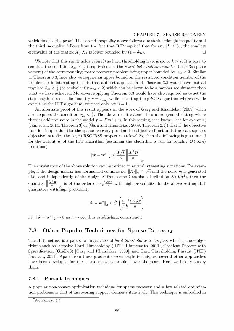
CHAPTER 7. SPARSE RECOVERYwhich finishes the proof. The second inequality above follows due to the triangle inequality andthe third inequality follows from the fact that RIP implies7 that for any |I| ≤ 3s, the smallesteigenvalue of the matrix X>I XI is lower bounded by (1− δ3s).
We note that this result holds even if the hard thresholding level is set to k > s. It is easy tosee that the condition δ3s <
12 is equivalent to the restricted condition number (over 3s-sparse
vectors) of the corresponding sparse recovery problem being upper bounded by κ3s < 3. Similarto Theorem 3.3, here also we require an upper bound on the restricted condition number of theproblem. It is interesting to note that a direct application of Theorem 3.3 would have insteadrequired δ2s <
13 (or equivalently κ2s < 2) which can be shown to be a harsher requirement than
what we have achieved. Moreover, applying Theorem 3.3 would have also required us to set thestep length to a specific quantity η = 1
1+δs while executing the gPGD algorithm whereas whileexecuting the IHT algorithm, we need only set η = 1.
An alternate proof of this result appears in the work of Garg and Khandekar [2009] whichalso requires the condition δ2s <
13 . The above result extends to a more general setting where
there is additive noise in the model y = Xw∗ + η. In this setting, it is known (see for example,[Jain et al., 2014, Theorem 3] or [Garg and Khandekar, 2009, Theorem 2.3]) that if the objectivefunction in question (for the sparse recovery problem the objective function is the least squaresobjective) satisfies the (α, β) RSC/RSS properties at level 2s, then the following is guaranteedfor the output w of the IHT algorithm (assuming the algorithm is run for roughly O (logn)iterations)
‖w−w∗‖2 ≤3√s
α
∥∥∥∥∥X>η
n
∥∥∥∥∥∞
The consistency of the above solution can be verified in several interesting situations. For exam-ple, if the design matrix has normalized columns i.e. ‖Xi‖2 ≤
√n and the noise ηi is generated
i.i.d. and independently of the design X from some Gaussian distribution N (0, σ2), then thequantity
∥∥∥X>ηn
∥∥∥∞
is of the order of σ√
log pn with high probability. In the above setting IHT
guarantees with high probability
‖w−w∗‖2 ≤ O
σα
√s log pn
,i.e. ‖w−w∗‖2 → 0 as n→∞, thus establishing consistency.
7.8 Other Popular Techniques for Sparse RecoveryThe IHT method is a part of a larger class of hard thresholding techniques, which include algo-rithms such as Iterative Hard Thresholding (IHT) [Blumensath, 2011], Gradient Descent withSparsification (GraDeS) [Garg and Khandekar, 2009], and Hard Thresholding Pursuit (HTP)[Foucart, 2011]. Apart from these gradient descent-style techniques, several other approacheshave been developed for the sparse recovery problem over the years. Here we briefly surveythem.
7.8.1 Pursuit Techniques
A popular non-convex optimization technique for sparse recovery and a few related optimiza-tion problems is that of discovering support elements iteratively. This technique is embodied in
7See Exercise 7.7.
88
7.8. OTHER POPULAR TECHNIQUES FOR SPARSE RECOVERYpursuit-style algorithms. We warn the reader that the popular Basis Pursuit algorithm is actu-ally a convex relaxation technique and not related to the other pursuit algorithms we discusshere. The terminology is a bit confusing but seems to be a matter of legacy.
The pursuit family of algorithms includes Orthogonal Matching Pursuit (OMP) [Troppand Gilbert, 2007], Orthogonal Matching Pursuit with Replacement (OMPR) [Jain et al.,2011], Compressive Sampling Matching Pursuit (CoSaMP) [Needell and Tropp, 2008], and theForward-backward (FoBa) algorithm [Zhang, 2011].
Pursuit methods work by gradually discovering the elements in the support of the truemodel vector w∗. At every time step, these techniques add a new support element to an activesupport set (which is empty to begin with) and solve a traditional least-squares problem onthe active support set. This least-squares problem has no sparsity constraints, and is hence aconvex problem which can be solved easily.
The support set is then updated by adding a new support element. It is common to addthe coordinate where the gradient of the objective function has the highest magnitude amongcoordinates not already in the support. FoBa-style techniques augment this method by havingbackward steps where support elements that were erroneously picked earlier are discarded whenthe error is detected.
Pursuit-style methods are, in general, applicable whenever the structure in the (non-convex)constraint set in question can be represented as a combination of a small number of atoms.Examples include sparse recovery, where the atoms are individual coordinates: every s-sparsevector is a linear combination of some s of these atoms.
Other examples include low-rank matrix recovery, which we will study in detail in § 8, wherethe atoms are rank-one matrices. The SVD theorem tells us that every r-rank matrix can indeedbe expressed as a sum of r rank-one matrices. There exist works [Tewari et al., 2011] that givegeneric methods to perform sparse recovery in such structurally constrained settings.
7.8.2 Convex Relaxation Techniques for Sparse Recovery
Convex relaxation techniques have been extremely popular for the sparse recovery problem. Infact they formed the first line of attack on non-convex optimization problems starting with theseminal work of Candès and Tao [2005], Candès et al. [2006], Donoho [2006] that, for the firsttime, established polynomial time, globally convergent solutions for the compressive sensingproblem.
A flurry of work then followed on relaxation-based techniques [Candès, 2008, Donoho et al.,2009, Foucart, 2010, Negahban et al., 2012] that vastly expanded the scope of the problemsbeing studied, the techniques being applied, as well as their analyses. It is important to notethat all methods, whether relaxation based or not, have to assume some design property suchas NSP/REP/RIP/RSC-RSS that we discussed earlier, in order to give provable guarantees.
The relaxation approach converts non-convex problems to convex problems first before solv-ing them. This approach, applied to the sparse regression problem, gives us the so-called LASSOproblem which has been studied extensively. Consider the sparse recovery problem ((SP-REG)).
minw∈Rp‖w‖0≤s
‖y−Xw‖22 .
Non-convexity arises in the problem due to the non-convex constraint ‖w‖0 ≤ s as the sparsityoperator is not a valid norm. The relaxation approach fixes this problem by changing theconstraint to use the L1 norm instead i.e.
minw∈Rp‖w‖1≤R
‖y−Xw‖22 , (LASSO-1)
89

CHAPTER 7. SPARSE RECOVERYor by using its regularized version instead
minw∈Rp
12n ‖y−Xw‖22 + λn ‖w‖1 . (LASSO-2)
The choice of the L1 norm is motivated mainly by its convexity as well as formal resultsthat assure us that the relaxation gap is small or non-existent. Both the above formulations((LASSO-1)) and ((LASSO-2)) are indeed convex but include parameters such as R and λnthat must be tuned properly to ensure proper convergence. Although the optimization problems((LASSO-1)) and ((LASSO-2)) are vastly different from ((SP-REG)), a long line of beautifulresults, starting from the seminal work of Candès and Tao [2005], Candès et al. [2006], Donoho[2006], showed that if the design matrix X satisfies RIP with appropriate constants, and ifthe parameters of the relaxations R and λn are appropriately tuned, then the solutions to therelaxations are indeed solutions to the original problems as well.
Below we state one such result from the recent text by Hastie et al. [2016]. We recommendthis text to any reader looking for a well-curated compendium of techniques and results on therelaxation approach to several non-convex optimization problems arising in machine learning.
Theorem 7.3. [Hastie et al., 2016, Theorem 11.1] Consider a sparse recovery problem y =Xw∗ + η where the model w∗ is s-sparse and the design matrix X satisfies the restricted-eigenvalue condition (see Definition 7.2) of the order s with constant α, then the followinghold
1. Any solution w1 to ((LASSO-1)) with R = ‖w∗‖1 satisfies
‖w1 −w∗‖2 ≤4α
√s
∥∥∥∥∥X>η
n
∥∥∥∥∥∞.
2. Any solution w2 to ((LASSO-2)) with λn ≥ 2∥∥∥X>η/n
∥∥∥∞
satisfies
‖w1 −w∗‖2 ≤3α
√sλn.
The reader can verify that the above bounds are competitive with the bounds for the IHTalgorithm that we discussed previously. We refer the reader to [Hastie et al., 2016, Chapter 11]for more consistency results for the LASSO formulations.
7.8.3 Non-convex Regularization Techniques
Instead of performing a complete convex relaxation of the problem, there exist approaches thatonly partly relax the problem. A popular approach in this direction uses Lq regularization with0 < q < 1 [Chartrand, 2007, Foucart and Lai, 2009, Wang et al., 2011]. The resulting problemstill remains non-convex but becomes a little well behaved in terms of having objective functionsthat are almost-everywhere differentiable. For instance, the following optimization problem maybe used to solve the noiseless sparse recovery problem.
minw∈Rp
‖w‖q ,
s.t. y = Xw
For noisy settings, one may replace the constraint with a soft constraint such as ‖y−Xw‖2 ≤ ε,or else move to an unconstrained version like LASSO with the L1 norm replaced by the Lq norm.
90
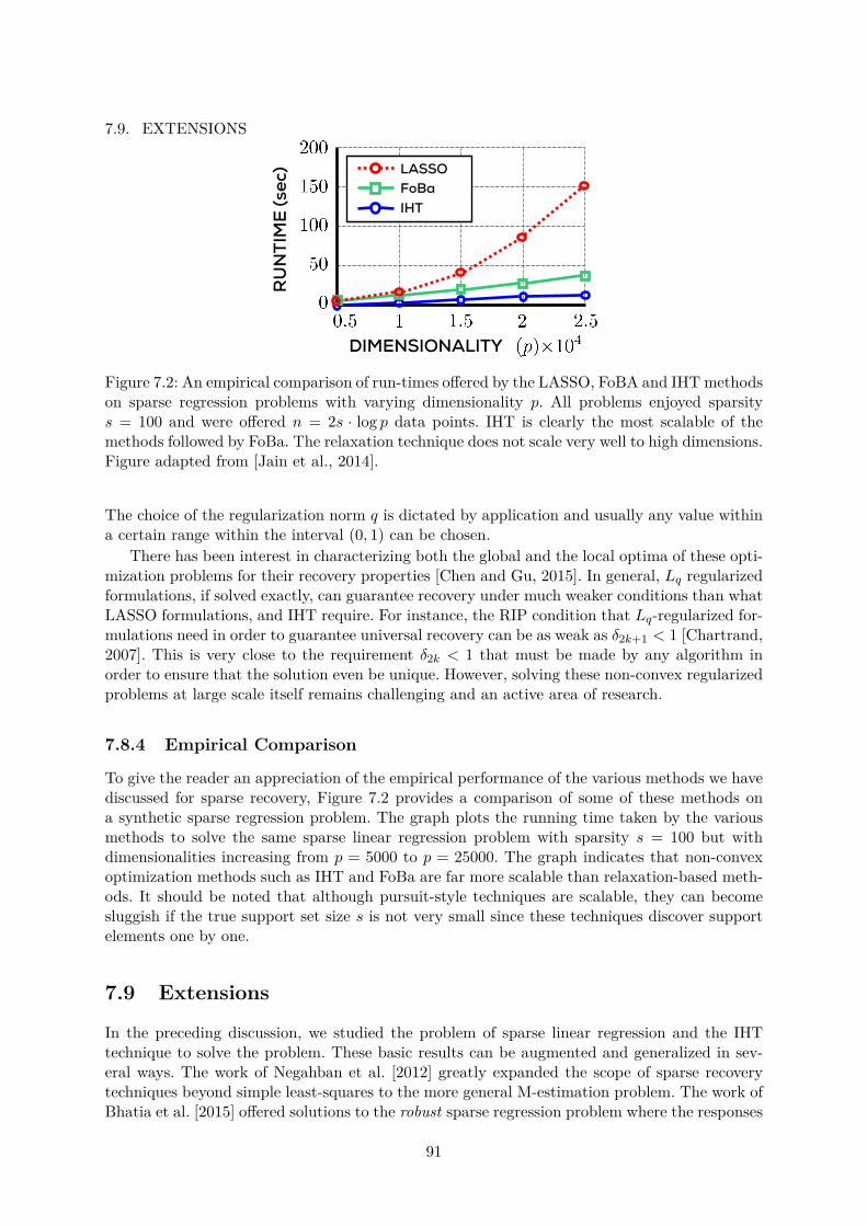
7.9. EXTENSIONS
DIMENSIONALITY
RU
NT
IME
(se
c) LASSO
FoBa
IHT
Figure 7.2: An empirical comparison of run-times offered by the LASSO, FoBA and IHT methodson sparse regression problems with varying dimensionality p. All problems enjoyed sparsitys = 100 and were offered n = 2s · log p data points. IHT is clearly the most scalable of themethods followed by FoBa. The relaxation technique does not scale very well to high dimensions.Figure adapted from [Jain et al., 2014].
The choice of the regularization norm q is dictated by application and usually any value withina certain range within the interval (0, 1) can be chosen.
There has been interest in characterizing both the global and the local optima of these opti-mization problems for their recovery properties [Chen and Gu, 2015]. In general, Lq regularizedformulations, if solved exactly, can guarantee recovery under much weaker conditions than whatLASSO formulations, and IHT require. For instance, the RIP condition that Lq-regularized for-mulations need in order to guarantee universal recovery can be as weak as δ2k+1 < 1 [Chartrand,2007]. This is very close to the requirement δ2k < 1 that must be made by any algorithm inorder to ensure that the solution even be unique. However, solving these non-convex regularizedproblems at large scale itself remains challenging and an active area of research.
7.8.4 Empirical Comparison
To give the reader an appreciation of the empirical performance of the various methods we havediscussed for sparse recovery, Figure 7.2 provides a comparison of some of these methods ona synthetic sparse regression problem. The graph plots the running time taken by the variousmethods to solve the same sparse linear regression problem with sparsity s = 100 but withdimensionalities increasing from p = 5000 to p = 25000. The graph indicates that non-convexoptimization methods such as IHT and FoBa are far more scalable than relaxation-based meth-ods. It should be noted that although pursuit-style techniques are scalable, they can becomesluggish if the true support set size s is not very small since these techniques discover supportelements one by one.
7.9 Extensions
In the preceding discussion, we studied the problem of sparse linear regression and the IHTtechnique to solve the problem. These basic results can be augmented and generalized in sev-eral ways. The work of Negahban et al. [2012] greatly expanded the scope of sparse recoverytechniques beyond simple least-squares to the more general M-estimation problem. The work ofBhatia et al. [2015] offered solutions to the robust sparse regression problem where the responses
91
CHAPTER 7. SPARSE RECOVERYmay be corrupted by an adversary. We will explore the robust regression problem in more detailin § 9. We discuss a few more such extensions below.
7.9.1 Sparse Recovery in Ill-Conditioned Settings
As we discussed before, the bound on the RIP constant δ3s <12 as required by Theorem 7.2,
effectively places a bound on the restricted condition number κ3s of the design matrix. In our casethe bound translates to κ3s = 1+δ3s
1−δ3s< 3. However, in cases such as the gene expression analysis
problem where the design matrix is not totally under our control, the restricted conditionnumber might be much larger than 3.
For instance, it can be shown that if the expression levels of two genes are highly correlatedthen this results in ill-conditioned design matrices. In such settings, it is much more appro-priate to assume that the design matrix satisfies restricted strong convexity and smoothness(RSC/RSS) which allows us to work with design matrices with arbitrarily large condition num-bers. It turns out that the IHT algorithm can be modified [see for example, Jain et al., 2014]to work in these ill-conditioned recovery settings.
Theorem 7.4. Suppose X ∈ Rn×p is a design matrix that satisfies the restricted strong convexityand smoothness property of order 2k+ s with constants α2k+s and β2k+s respectively. Let w∗ ∈B0(s) ⊂ Rp be any arbitrary sparse vector and let y = Xw∗. Then the IHT algorithm, whenexecuted with a step length η < 2
β2k+s, and a projection sparsity level k ≥ 32
(β2k+sα2k+s
)2s, ensures∥∥wt −w∗
∥∥2 ≤ ε after t = O
(β2k+sα2k+s
log ‖w∗‖2ε
)iterations of the algorithm.
Note that the above result does not place any restrictions on the condition number or theRSC/RSS constants of the problem. The result also mimics Theorem 3.3 in its dependence onthe (restricted) condition number of the optimization problem i.e. κ2k+s = β2k+s
α2k+s. The proof of
this result is a bit tedious, hence omitted.
7.9.2 Recovery from a Union of Subspaces
If we look closely, the set B0(s) is simply a union of(ps
)linear subspaces, each subspace encoding
a specific sparsity pattern. It is natural to wonder whether the methods and analyses describedabove also hold when the vector to be recovered belongs to a general union of subspaces.More specifically, consider a family of linear subspaces H1, . . . ,HL ⊂ Rp and denote the unionof these subspaces by H =
⋃Li=1Hi. The restricted strong convexity and restricted strong
smoothness conditions can be appropriately modified to suit this setting by requiring a designmatrix X : Rp → Rn to satisfy, for every w1,w2 ∈ H,
α · ‖w1 −w2‖22 ≤ ‖X(w1 −w2)‖22 ≤ L · ‖w1 −w2‖22
It turns out that IHT, with an appropriately modified projection operator ΠH(·), can ensurerecovery of vectors that are guaranteed to reside in a small union of low-dimensional subspaces.Moreover, a linear rate of convergence, as we have seen for the IHT algorithm in the sparseregression case, can still be achieved. We refer the reader to the work of Blumensath [2011] formore details of this extension.
7.9.3 Dictionary Learning
A very useful extension of sparse recovery, or sparse coding emerges when we attempt to learnthe design matrix as well. Thus, all we are given are observations y1, . . . ,ym ∈ Rn and wewish to learn a design matrix X ∈ Rn×p such that the observations yi can be represented as
92
7.10. EXERCISESsparse combinations wi ∈ Rp of the columns of the design matrix i.e. yi ≈ Xwi such that‖wi‖0 ≤ s p. The problem has several applications in the fields of computer vision and signalprocessing and has seen a lot of interest in the recent past.
The alternating minimization technique where one alternates between estimating the designmatrix and the sparse representations, is especially popular for this problem. Methods mostlydiffer in the exact implementation of these alternations. Some notable works in this area include[Agarwal et al., 2016, Arora et al., 2014, Gribonval et al., 2015, Spielman et al., 2012].
7.10 ExercisesExercise 7.1. Suppose a design matrix X ∈ Rn×p satisfies Xw1 = Xw2 for some w1 6= w2 ∈Rp. Then show that there exists an entire subspace H ⊂ Rp such that for all w,w′ ∈ H, we haveXw = Xw′.
Exercise 7.2. Show that the set C(k) :=⋃S:|S|=k C(S) is non-convex.
Exercise 7.3. Show that if a design matrix X satisfies the null-space property of order 2s,then for any two distinct s-sparse vectors v1,v2 ∈ B0(s), v1 6= v2, it must be the case thatXv1 6= Xv2.
Exercise 7.4. Show that the RSC/RSS notion introduced in Definition 7.4 is equivalent to theRSC/RSS notion in Definition 3.2 defined in § 3 for an appropriate choice of function andconstraint sets.
Exercise 7.5. Show that RSC-RSS ⇒ REP ⇒ NSP i.e. a matrix that satisfies the RSC/RSScondition for some constants, must satisfy the REP condition for some constants which in turnmust force it to satisfy the null-space property.
Exercise 7.6. Show that every µ-incoherent matrix satisfies the RIP property at order k withparameter δ = (k − 1)µ.
Exercise 7.7. Suppose the matrix X ∈ Rn×p satisfies RIP at order s with constant δs. Thenshow that for any set I ⊂ [p], |I| ≤ s, the smallest eigenvalue of the matrix X>I XI is lowerbounded by (1− δs).
Exercise 7.8. Show that the RIP constant is monotonic in its order i.e. if a matrix X satisfiesRIP of order k with constant δk, then it also satisfies RIP for all orders k′ ≤ k with δk′ ≤ δk.
7.11 Bibliographic NotesThe literature on sparse recovery techniques is too vast for this note to cover. We have alreadycovered several directions in §§ 7.8 and 7.9 and point the reader to references therein.
93
The official publication is available from now publishers viahttp://dx.doi.org/10.1561/2200000058
Chapter 8
Low-rank Matrix Recovery
In this section, we will look at the problem of low-rank matrix recovery in detail. Althoughsimple to motivate as an extension of the sparse recovery problem that we studied in § 7, theproblem rapidly distinguishes itself in requiring specific tools, both algorithmic and analytic.We will start our discussion with a milder version of the problem as a warm up and move onto the problem of low-rank matrix completion which is an active area of research.
8.1 Motivating Applications
We will take the following two running examples to motivate the problem of low-rank matrixrecovery.
Collaborative Filtering Recommendation systems are popularly used to model the preferencepatterns of users, say at an e-commerce website, for items being sold on that website, althoughthe principle of recommendation extends to several other domains that demand personalizationsuch as education and healthcare. Collaborative filtering is a popular technique for buildingrecommendation systems.
The collaborative filtering approach seeks to exploit co-occurring patterns in the observedbehavior across users in order to predict future user behavior. This approach has proven suc-cessful in addressing users that interact very sparingly with the system. Consider a set of musers u1, . . . , um, and n items a1, . . . , an. Our goal is to predict the preference score s(i,j) thatis indicative of the interest user ui has in item aj .
However, we get direct access to (noisy estimates of) actual preference scores for only a fewitems per user by looking at clicks, purchases etc. That is to say, if we consider the m × npreference matrix A = [Aij ] where Aij = s(i,j) encodes the (true) preference of the ith user forthe jth item, we get to see only k m ·n entries of A, as depicted in Figure 8.1. Our goal is torecover the remaining entries.
The problem of paucity of available data is readily apparent in this setting. In its nascentform, the problem is not even well posed and does not admit a unique solution. A popular wayof overcoming these problems is to assume a low-rank structure in the preference matrix.
As we saw in Exercise 3.3, this is equivalent to assuming that there is an r-dimensionalvector ui denoting the ith user and an r-dimensional vector aj denoting the jth such thats(i,j) ≈ 〈ui,aj〉. Thus, if Ω ⊂ [m] × [n] is the set of entries that have been observed by us,then the problem of recovering the unobserved entries can be cast as the following optimizationproblem:
minX∈Rm×nrank(X)≤r
∑(i,j)∈Ω
(Xij −Aij)2 .
94
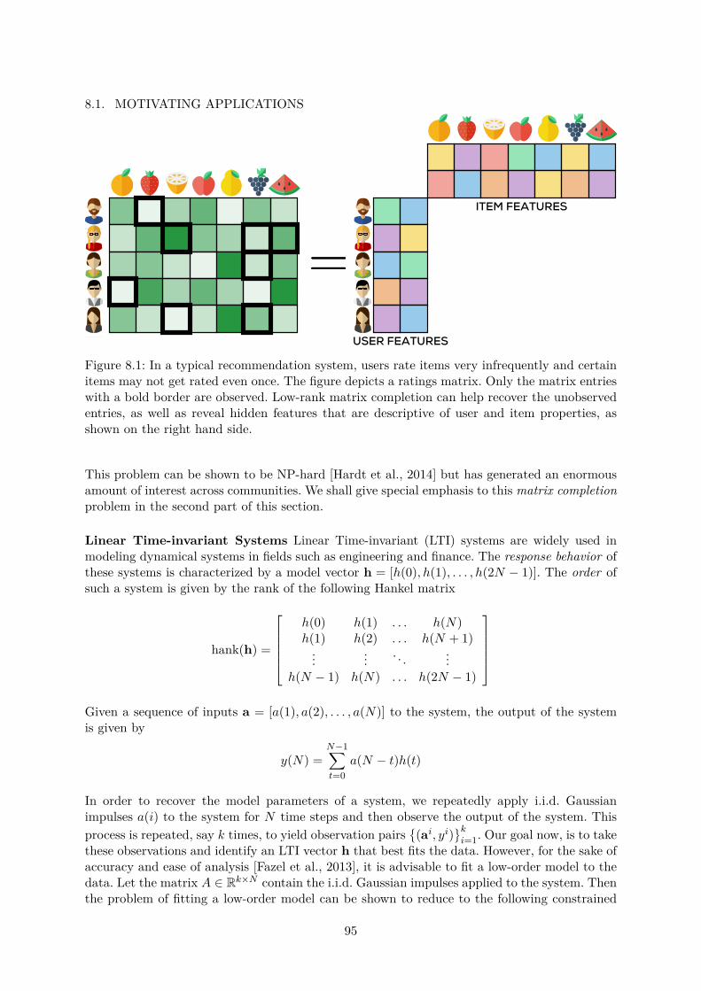
8.1. MOTIVATING APPLICATIONS
ITEM FEATURES
USER FEATURES
Figure 8.1: In a typical recommendation system, users rate items very infrequently and certainitems may not get rated even once. The figure depicts a ratings matrix. Only the matrix entrieswith a bold border are observed. Low-rank matrix completion can help recover the unobservedentries, as well as reveal hidden features that are descriptive of user and item properties, asshown on the right hand side.
This problem can be shown to be NP-hard [Hardt et al., 2014] but has generated an enormousamount of interest across communities. We shall give special emphasis to this matrix completionproblem in the second part of this section.
Linear Time-invariant Systems Linear Time-invariant (LTI) systems are widely used inmodeling dynamical systems in fields such as engineering and finance. The response behavior ofthese systems is characterized by a model vector h = [h(0), h(1), . . . , h(2N − 1)]. The order ofsuch a system is given by the rank of the following Hankel matrix
hank(h) =
h(0) h(1) . . . h(N)h(1) h(2) . . . h(N + 1)...
... . . . ...h(N − 1) h(N) . . . h(2N − 1)
Given a sequence of inputs a = [a(1), a(2), . . . , a(N)] to the system, the output of the systemis given by
y(N) =N−1∑t=0
a(N − t)h(t)
In order to recover the model parameters of a system, we repeatedly apply i.i.d. Gaussianimpulses a(i) to the system for N time steps and then observe the output of the system. Thisprocess is repeated, say k times, to yield observation pairs
(ai, yi)
ki=1. Our goal now, is to take
these observations and identify an LTI vector h that best fits the data. However, for the sake ofaccuracy and ease of analysis [Fazel et al., 2013], it is advisable to fit a low-order model to thedata. Let the matrix A ∈ Rk×N contain the i.i.d. Gaussian impulses applied to the system. Thenthe problem of fitting a low-order model can be shown to reduce to the following constrained
95
CHAPTER 8. LOW-RANK MATRIX RECOVERYoptimization problem with a rank objective and an affine constraint.
min rank(hank(h))s.t. Ah = y,
The above problem is a non-convex optimization problem due to the objective being the min-imization of the rank of a matrix. Several other problems in metric embedding and multi-dimensional scaling, image compression, low rank kernel learning and spatio-temporal imagingcan also be reduced to low rank matrix recovery problems [Jain et al., 2010, Recht et al., 2010].
8.2 Problem FormulationThe two problems considered above can actually be cast in a single problem formulation, thatof Affine Rank Minimization (ARM). Consider a low rank matrix X∗ ∈ Rm×n that we wishto recover and an affine transformation A : Rm×n → Rk. The transformation can be seen asa concatenation of k real valued affine transformations Ai : Rm×n → R. We are given thetransformation A, and its (possibly noisy) action y = A(X∗) ∈ Rk on the matrix X∗ and ourgoal is to recover this matrix by solving the following optimization problem.
min rank(X)s.t. A(X) = y, (ARM)
This problem can be shown to be NP-hard due to a reduction to the sparse recovery problem1.The LTI modeling problem can be easily seen to be an instance of ARM with the Gaussianimpulses being delivered to the system resulting in a k-dimensional affine transformation ofthe Hankel matrix corresponding to the system. However, the Collaborative Filtering problemis also an instance of ARM. To see this, for any (i, j) ∈ [m] × [n], let O(i,j) ∈ Rm×n be thematrix such that its (i, j)-th entry O(i,j)
ij = 1 and all other entries are zero. Then, simply definethe affine transformation A(i,j) : X 7→ tr(X>O(i,j)) = Xij . Thus, if we observe k user-itemratings, the ARM problem effectively operates with a k-dimensional affine transformation ofthe underlying rating matrix.
Due to its similarity to the sparse recovery problem, we will first discuss the general ARMproblem. However, we will find it beneficial to cast the collaborative filtering problem as aLow-rank Matrix Completion problem instead. In this problem, we have an underlying low rankmatrix X∗ of which, we observe entries in a set Ω ⊂ [m]× [n]. Then the low rank matrixcompletion problem can be stated as
minX∈Rm×nrank(X)≤r
‖ΠΩ(X −X∗)‖2F , (LRMC)
where ΠΩ(X) is defined, for any matrix X as
ΠΩ(X)i,j =Xi,j if (i, j) ∈ Ω
0 otherwise.
The above formulation succinctly captures our objective to find a completion of the ratingsmatrix that is both, low rank, as well as agrees on the user ratings that are actually observed.As pointed out earlier, this problem is NP-hard [Hardt et al., 2014].
Before moving on to present algorithms for the ARM and LRMC problems, we discuss somematrix design properties that would be required in the convergence analyses of the algorithms.
1See Exercise 8.1.
96

8.3. MATRIX DESIGN PROPERTIES8.3 Matrix Design Properties
Similar to sparse recovery, there exist design properties that ensure that the general NP-hardnessof the ARM and LRMC problems can be overcome in well-behaved problem settings. In factgiven the similarity between ARM and sparse recovery problems, it is tempting to try andimport concepts such as RIP into the matrix-recovery setting.
In fact this is exactly the first line of attack that was adopted in literature. What followedwas a beautiful body of work that generalized, both structural notions such as RIP, as wellas algorithmic techniques such as IHT, to address the ARM problem. Given the generality ofthese constructs, as well as the smooth transition it offers having studied sparse recovery, wefeel compelled to present them to the reader.
8.3.1 The Matrix Restricted Isometry Property
The generalization of RIP to matrix settings, referred to as matrix RIP, follows in a relativelystraightforward manner and was first elucidated by Recht et al. [2010]. Quite in line with thesparse recovery setting, the intuition dictates that recovery should be possible only if the affinetransformation does not identify two distinct low-rank matrices. A more robust version dictatesthat no low-rank matrix should be distorted significantly by this transformation which gives usthe following.
Definition 8.1 (Matrix Restricted Isometry Property [Recht et al., 2010]). A linear map A :Rm×n → Rk is said to satisfy the matrix restricted isometry property of order r with constantδr ∈ [0, 1) if for all matrices X of rank at most r, we have
(1− δr) · ‖X‖2F ≤ ‖A(X)‖22 ≤ (1 + δr) · ‖X‖2F .
Furthermore, the work of Recht et al. [2010] also showed that linear maps or affine transfor-mations arising in random measurement models, such as those in image compression and LTIsystems, do satisfy RIP with requisite constants whenever the number of affine measurementssatisfies k = O (nr) [Oymak et al., 2015]. Note however, that these are settings in which the de-sign of the affine map is within our control. For settings, where the restricted condition numberof the affine map is not within our control, more involved analysis is required. The bibliographicnotes point to some of these results.
Given the relatively simple extension of the RIP definitions to the matrix setting, it isall the more tempting to attempt to apply gPGD-style techniques to solve the ARM problem,particularly since we saw how IHT succeeded in offering scalable solutions to the sparse recoveryproblem. The works of [Goldfarb and Ma, 2011, Jain et al., 2010] showed that this is indeedpossible. We will explore this shortly.
8.3.2 The Matrix Incoherence Property
We begin this discussion by warning the reader that there are two distinct notions prevalent inliterature, both of which are given the same name, that of the matrix incoherence property. Thefirst of these notions was introduced in § 7.6 as a property that can be used to ensure the RIPproperty in matrices. However a different property, but bearing the same name, finds applicationin matrix completion problems which we now introduce. We note that the two properties arenot known to be strongly related in a formal sense and the coincidental clash of the namesseems to be a matter of legacy.
Nevertheless, the intuition behind the second notion of matrix incoherence is similar to thatfor RIP in that it seeks to make the problem well posed. Consider the matrix A =
∑rt=1 st ·
97
CHAPTER 8. LOW-RANK MATRIX RECOVERYAlgorithm 9 Singular Value Projection (SVP)Input: Linear map A, measurements y, target rank q, step length ηOutput: A matrix X with rank at most q1: X1 ← 0m×n2: for t = 1, 2, . . . do3: Y t+1 ← Xt − η · A>(A(Xt)− y)4: Compute top q singular vectors/values of Y t+1: U tq ,Σt
q, Vtq
5: Xt+1 ← U tqΣtq(V t
q )>6: end for7: return Xt
eite>jt ∈ Rm×n where ei are the canonical orthonormal vectors in Rm and ej are the canonicalorthonormal vectors in Rn. Clearly A has rank at most r.
However, this matrix A is non-zero only at r locations. Thus, it is impossible to recover theentire matrix uniquely unless these very r locations (it, jt)t=1,...,r are actually observed. Sincein recommendation settings, we only observe a few random entries of the matrix, there is a goodpossibility that none of these entries will ever be observed. This presents a serious challengefor the matrix completion problem – the low rank structure is not sufficient to ensure uniquerecovery!
To overcome this and make the LRMC problem well posed with a unique solution, anadditional property is imposed. This so-called matrix incoherence property prohibits low rankmatrices that are also sparse. A side effect of this imposition is that for incoherent matrices,observing a small random set of entries is enough to uniquely determine the unobserved entriesof the matrix.
Definition 8.2 (Matrix Incoherence Property [Candès and Recht, 2009]). A matrix A ∈ Rm×nof rank r is said to be incoherent with parameter µ if its left and right singular matrices havebounded row norms. More specifically, let A = UΣV > be the SVD of A. Then µ-incoherencedictates that
∥∥U i∥∥2 ≤µ√r√m
for all i ∈ [m] and∥∥V j
∥∥2 ≤
µ√r√n
for all j ∈ [n]. A stricter versionof this property requires all entries of U to satisfy |Uij | ≤ µ√
mand all entries of V to satisfy
|Vij | ≤ µ√n.
A low rank incoherent matrix is guaranteed to be far, i.e., well distinguished, from any sparsematrix, something that is exploited by algorithms to give guarantees for the LRMC problem.
8.4 Low-rank Matrix Recovery via Proj. Gradient Descent
We will now apply the gPGD algorithm to the ARM problem. To do so, first consider thefollowing reformulation of the ARM problem to make it more compatible to the projectedgradient descent iterations.
min 12 ‖A(X)− y‖22
s.t. rank(X) ≤ r (ARM-2)
Applying the gPGD algorithm to the above formulation gives us the Singular Value Projection(SVP) algorithm (Algorithm 9). Note that in this case, the projection needs to be carried outonto the set of low rank matrices. However, as we saw in § 3.1, this can be efficiently done bycomputing the singular value decomposition of the iterates.
SVP offers ease of implementation and speed similar to IHT. Moreover, it applies to ARMproblems in general. If the Matrix RIP property is appropriately satisfied, then SVP guarantees
98
8.5. A LOW-RANK MATRIX RECOVERY GUARANTEE FOR SVPa linear rate of convergence to the optimum, much like IHT. All these make SVP a very attractivechoice for solving low rank matrix recovery problems.
Below, we give a convergence proof for SVP in the noiseless case, i.e., when y = A(X∗).The proof is similar in spirit to the convergence proof we saw for the IHT algorithm in § 7 butdiffers in crucial aspects since sparsity in this case is apparent not in the signal domain (thematrix is not itself sparse) but the spectral domain (the set of singular values of the matrix issparse). The analysis can be extended to noisy measurements as well and can be found in [Jainet al., 2010].
8.5 A Low-rank Matrix Recovery Guarantee for SVPWe will now present a convergence result for the SVP algorithm. As before, although the generalconvergence result for gPGD can indeed be applied here, we will see, just as we did in § 7, thatthe problem specific analysis we present here is finer and reveals more insights about the ARMproblem structure.
Theorem 8.1. Suppose A : Rm×n → Rk is an affine transformation that satisfies the matrixRIP property of order 2r with constant δ2r ≤ 1
3 . Let X∗ ∈ Rm×n be a matrix of rank at most r
and let y = A(X∗). Then the SVP Algorithm (Algorithm 9), when executed with a step lengthη = 1/(1 + δ2r), and a target rank q = r, ensures
∥∥Xt −X∗∥∥2F ≤ ε after t = O
(log ‖y‖
22
2ε
)iterations of the algorithm.
Proof. Notice that the notions of sparsity and support are very different in ARM than what theywere for sparse regression. Consequently, the exact convergence proof for IHT (Theorem 7.2)is not applicable here. We will first establish an intermediate result that will show, that aftert = O
(log ‖y‖
22
2ε
)iterations, SVP ensures
∥∥A(Xt)− y∥∥2
2 ≤ ε. We will then use the matrix RIPproperty (Definition 8.1) to deduce∥∥∥A(Xt)− y
∥∥∥2
2=∥∥∥A(Xt −X∗)
∥∥∥2
2≥ (1− δ2r) ·
∥∥∥Xt −X∗∥∥∥2
F,
which will conclude the proof. To prove this intermediate result, let us denote the objectivefunction as
f(X) = 12 ‖A(X)− y‖22 = 1
2 ‖A(X −X∗)‖22 .
An application of the matrix RIP property then gives us
f(Xt+1)
= f(Xt) +⟨A(Xt −X∗),A(Xt+1 −Xt)
⟩+ 1
2
∥∥∥A(Xt+1 −Xt)∥∥∥2
2
≤ f(Xt) +⟨A(Xt −X∗),A(Xt+1 −Xt)
⟩+ (1 + δ2r)
2
∥∥∥Xt+1 −Xt∥∥∥2
F.
The following steps now introduce the intermediate variable Y t+1 into the analysis in order tolink the successive iterates by using the fact that Xt+1 was the result of a non-convex projectionoperation. ⟨
A(Xt −X∗),A(Xt+1 −Xt)⟩
+ (1 + δ2r)2 ·
∥∥∥Xt+1 −Xt∥∥∥2
F
= 1 + δ2r2 ·
∥∥∥Xt+1 − Y t+1∥∥∥2
F− 1
2(1 + δ2r)·∥∥∥A>(A(Xt −X∗))
∥∥∥2
F
99
CHAPTER 8. LOW-RANK MATRIX RECOVERYAlgorithm 10 AltMin for Matrix Completion (AM-MC)Input: Matrix A ∈ Rm×n of rank r observed at entries in the set Ω, sampling probability p,
stopping time TOutput: A matrix X with rank at most r1: Partition Ω into 2T + 1 sets Ω0,Ω1, . . . ,Ω2T uniformly and randomly2: U1 ← SVD(1
pΠΩ0(A), r), the top r left singular vectors of 1pΠΩ0(A)
3: for t = 1, 2, . . . , T do4: V t+1 ← arg minV ∈Rn×r
∥∥∥ΠΩt(U tV > −A)∥∥∥2
F
5: U t+1 ← arg minU∈Rm×r∥∥∥ΠΩT+t(U(V t+1)> −A)
∥∥∥2
F6: end for7: return U>(V >)>
≤ 1 + δ2r2 ·
∥∥∥X∗ − Y t+1∥∥∥2
F− 1
2(1 + δ2r)·∥∥∥A>(A(Xt −X∗))
∥∥∥2
F
=⟨A(Xt −X∗),A(X∗ −Xt)
⟩+ (1 + δ2r)
2 ·∥∥∥X∗ −Xt
∥∥∥2
F
≤⟨A(Xt −X∗),A(X∗ −Xt)
⟩+ (1 + δ2r)
2(1− δ2r)·∥∥∥A(X∗ −Xt)
∥∥∥2
2
= −f(Xt)− 12
∥∥∥A(X∗ −Xt)∥∥∥2
2+ (1 + δ2r)
2(1− δ2r)·∥∥∥A(X∗ −Xt)
∥∥∥2
2.
The first step uses the identity Y t+1 = Xt− η · A>(A(Xt)−y) from Algorithm 9, the fact thatwe set η = 1
1+δ2r, and elementary rearrangements. The second step follows from the fact that∥∥Xt+1 − Y t+1∥∥2
F ≤∥∥X∗ − Y t+1∥∥2
F by virtue of the SVD step which makes Xt+1 the best rank-(2r) approximation to Y t+1 in terms of the Frobenius norm. The third step simply rearrangesthings in the reverse order of the way they were arranged in the first step, the fourth stepuses the matrix RIP property and the fifth step makes elementary manipulations. This, uponrearrangement, and using
∥∥A(Xt −X∗)∥∥2
2 = 2f(Xt), gives us
f(Xt+1) ≤ 2δ2r1− δ2r
· f(Xt).
Since f(X1) = ‖y‖22, as we set X1 = 0m×n, if δ2r < 1/3 (i.e., 2δ2r1−δ2r
< 1), we have the claimedconvergence result.
One can, in principle, apply the SVP technique to the matrix completion problem as well.However, on the LMRC problem, SVP is outperformed by gAM-style approaches which we studynext. Although the superior performance of gAM on the LMRC problem was well documentedempirically, it took some time before a theoretical understanding could be obtained. This wasfirst done in the works of Keshavan [2012], Jain et al. [2013]. These results set off a long line ofworks that progressively improved both the algorithm, as well as its analysis.
8.6 Matrix Completion via Alternating Minimization
We will now look at the alternating minimization technique for solving the low-rank matrixcompletion problem. As we have observed before, the LRMC problem admits an equivalentreformulation where the low rank structure constraint is eliminated and instead, the solution is
100
8.7. A LOW-RANK MATRIX COMPLETION GUARANTEE FOR AM-MCdescribed in terms of two low-rank components
minU∈Rm×kV ∈Rn×k
∥∥∥ΠΩ(UV > −X∗)∥∥∥2
F. (LRMC*)
In this case, fixing either U or V reduces the above problem to a simple least squares problem forwhich we have very efficient and scalable solvers. As we saw in § 4, such problems are excellentcandidates for the gAM algorithm to be applied. The AM-MC algorithm (see Algorithm 10)applies the gAM approach to the reformulated LMRC problem. The AM-MC approach is thechoice of practitioners in the context of collaborative filtering [Chen and He, 2012, Koren et al.,2009, Zhou et al., 2008]. However, AM-MC, like other gAM-style algorithms, does require properinitialization and tuning.
8.7 A Low-rank Matrix Completion Guarantee for AM-MCWe will now analyze the convergence properties of the AM-MC method for matrix completion.To simplify the presentation, we will restrict ourselves to the case when the matrix A ∈ Rm×nis rank one. This will allow us to present the essential arguments without getting involved withtechnical details. Let A = u∗(v∗)> be a µ-incoherent matrix that needs to be recovered, where‖u∗‖2 = ‖v∗‖2 = 1. It is easy to see that µ-incoherence implies ‖u∗‖∞ ≤
µ√m
and ‖v∗‖∞ ≤µ√n.
We will also assume the Bernoulli sampling model i.e., that the set of observed indices Ω isgenerated by selecting each entry (i, j) for inclusion in Ω in an i.i.d. fashion with probability p.More specifically, (i, j) ∈ Ω iff δij = 1 where δij = 1 with probability p and 0 otherwise.
For simplicity, we will assume that each iteration of the AM-MC procedure receives afresh set of samples Ω from A. This can be achieved in practice by randomly partitioning theavailable set of samples into as many groups as the iterations of the procedure. The completionguarantee will proceed in two steps. In the first step, we will show that the initialization stepin Algorithm 10 itself brings AM-MC within a constant distance of the optimal solution. Next,we will show that this close initialization is sufficient for AM-MC to ensure a linear rate ofconvergence to the optimal solution.
Initialization: We will now show that the initialization step (Step 2 in Algorithm 10) providesa point (u1,v1) which is at most a constant c > 0 distance away from (u∗,v∗). To this we needa Bernstein-style argument which we provide here for the rank-1 case.
Theorem 8.2. [Tropp, 2012, Theorem 1.6] Consider a finite sequence Zk of independentrandom matrices of dimension m× n. Assume each matrix satisfies E [Zk] = 0 and ‖Zk‖2 ≤ Ralmost surely and denote
σ2 := max∥∥∥∑k ZkZ
>k
∥∥∥2,∥∥∥∑k Z
>k Zk
∥∥∥2
.
Then, for all t ≥ 0, we have
P [‖∑k Zk‖2 ≥ t] ≤ (m+ n) · exp
(−t2
σ2+Rt/3
).
Below we apply this inequality to analyze the initialization step for AM-MC in the rank-1 case. We point the reader to [Recht, 2011] and [Keshavan et al., 2010] for a more preciseargument analyzing the initialization step in the general rank-r case.
Theorem 8.3. For a rank one matrix A satisfying the µ-incoherence property, let the observedsamples Ω be generated with sampling probability p as described above. Let u1,v1 be the singular
101
CHAPTER 8. LOW-RANK MATRIX RECOVERYvectors of 1
pPΩ(A) corresponding to its largest singular value. Then for any ε > 0, if p ≥45µ2
ε2 ·log(m+n)minm,n , then with probability at least 1− 1/(m+ n)10:∥∥∥∥1
pΠΩ(A)−A
∥∥∥∥2≤ ε,
∥∥∥u1 − u∗∥∥∥
2≤ ε,
∥∥∥v1 − v∗∥∥∥
2≤ ε.
Moreover, the vectors u1 and v1 are also 2µ-incoherent.
Proof. Notice that the statement of the theorem essentially states that once enough entries inthe matrix have been observed (as dictated by the requirement p ≥ 45µ2
ε2 ·log(m+n)minm,n) an SVD step
on the incomplete matrix will yield components u1,v1 that are very close to the components ofthe complete matrix u∗,v∗. Moreover, since u∗,v∗ are incoherent by assumption, the estimatedcomponents u1,v1 will be so too.
To apply Theorem 8.2 to prove this result, we will first express 1pΠΩ(A) as a sum of random
matrices. We first rewrite 1pΠΩ(A) = 1
p
∑ij δijAijeie>j =
∑ijWij where δij = 1 if (i, j) ∈ Ω
and 0 otherwise. Note that the Bernoulli sampling model assures us that the random variablesWij = 1
pδijAijeie>j are independent and that E [δij ] = p. This gives us E [Wij ] = Aijeie>j . Note
that∑ij Aijeie>j = A.
The matrices Zij = Wij − Aijeie>j shall serve as our random matrices in the applicationof Theorem 8.2. Clearly E [Zij ] = 0. We also have maxij ‖Wij‖2 ≤ 1
p maxij |Aij | ≤ µ2
p√mn
due to the incoherence assumption. Applying the triangle inequality gives us maxij ‖Zij‖2 ≤maxij ‖Wij‖2 + maxij ‖Aijeie>j ‖2 ≤
(1 + 1
p
)µ2√mn≤ 2µ2
p√mn
.
Moreover, as Aij = u∗iv∗j and ‖v∗‖2 = 1, we have E[∑
ijWijW>ij
]= 1
p
∑i
∑j A
2ijeie>i =
1p
∑i(u∗i )2eie>i . Due to incoherence ‖u∗‖∞ ≤
µ√m, we get
∥∥∥E [∑ijWijW>ij
]∥∥∥2≤ µ2
p·m , which canbe shown to give us ∥∥∥∥∥∥E
∑ij
ZijZ>ij
∥∥∥∥∥∥2
≤(1p− 1
)· µ
2
m≤ µ2
p ·m
Similarly, we can also get∥∥∥E [∑ij Z
>ijZij
]∥∥∥2≤ µ2
p·n . Now using Theorem 8.2 gives us, withprobability at least 1− δ,∥∥∥∥1
pΠΩ(A)−A
∥∥∥∥2≤ 2µ2
3p√mn
log[m+ n
δ
]+√
µ2
p ·min m,n log[m+ n
δ
]
If p ≥ 45µ2 log(m+n)ε2·minm,n , we have with probability at least 1− 1/(m+ n)10,∥∥∥∥1
pΠΩ(A)−A
∥∥∥∥2≤ ε.
The proof now follows by applying the Davis-Kahan inequality [Golub and Loan, 1996] with theabove bound. It can be shown [Jain and Netrapalli, 2015] that the vectors that are recoveredas a result of this initialization are incoherent as well.
Linear Convergence: We will now show that, given the initialization above, the AM-MCprocedure converges to the true solution with a linear rate of convergence. This will involveshowing a few intermediate results, such as showing that the alternation steps preserve incoher-ence. Since the Theorem 8.3 shows that u1 is 2µ-incoherent, this will establish the incoherenceof all future iterates. Preserving incoherence will be crucial in showing the next result which
102
8.7. A LOW-RANK MATRIX COMPLETION GUARANTEE FOR AM-MCshows that successive iterates get increasingly close to the optimum. Put together, these willestablish the convergence result. First, recall that in the tth iteration of the AM-MC algorithm,vt+1 is updated as
vt+1 = arg minv
∑ij
δij(utivj − u∗iv∗j )2,
which gives us
vt+1j =
∑i δiju∗iuti∑i δij(uti)2 · v
∗j . (8.1)
Note that this means that if u∗ = ut, then vt+1 = v∗. Also, note that if δij = 1 for all (i, j)which happens when the sampling probability satisfies p = 1, we have vt+1 = 〈u
t,u∗〉‖ut‖2
2· v∗. This
is reminiscent of the power method used to recover the leading singular vectors of a matrix.Indeed if we let u = ut/
∥∥ut∥∥2, we get∥∥ut∥∥2 · v
t+1 = 〈u,u∗〉 · v∗ if p = 1.This allows us to rewrite the update (8.1) as a noisy power update.∥∥∥ut∥∥∥
2· vt+1 = 〈u,u∗〉 · v∗ −B−1(〈u,u∗〉B − C)v∗ (8.2)
where B,C ∈ Rn×n are diagonal matrices with Bjj = 1p
∑i δij(ui)2 and Cjj = 1
p
∑i δijuiu∗i . The
following two lemmata show that if ut is 2µ incoherent and if p is large enough, then: a) vt+1
is also 2µ incoherent, and b) the angular distance between vt+1 and v∗ decreases as comparedto that between ut and u∗. The following lemma will aid the analysis.
Lemma 8.4. Suppose a,b ∈ Rn are two fixed µ-incoherent unit vectors. Also suppose δi, i ∈ [n]are i.i.d. Bernoulli random variables such that δi = 1 with probability p and 0 otherwise. Then,for any ε > 0, if p > 27µ2 logn
nε2 , then with probability at least 1−1/n10,∣∣∣1p∑i δiaibi − 〈a,b〉
∣∣∣ ≤ ε.Proof. Define Zi =
(δip − 1
)aibi. Using the incoherence of the vectors, we get E [Zi] = 0,∑n
i=1 E[Z2i
]=(
1p − 1
)∑ni=1(aibi)2 ≤ µ2
pn since ‖b‖2 = 1, and |Zi| ≤ µ2
pn almost surely. Applyingthe Bernstein inequality gives us
P[∣∣∣∣∣1p∑
i
δiaibi − 〈a,b〉∣∣∣∣∣ > t
]≤ exp
(−3pnt2
6µ4 + 2µ2t
),
which upon simple manipulations, gives us the result.
Lemma 8.5. With probability at least min1− 1/n10, 1− 1/m10, if a pair of iterates (ut,vt)
in the execution of the AM-MC procedure are 2µ-incoherent, then so are the next pair of iterates(ut+1,vt+1).
Proof. Since ‖u‖2 = 1, using Lemma 8.4 tells us that with high probability, for all j, we have|Bjj − 1| ≤ ε as well as |Cjj − 〈u,u∗〉| ≤ ε. Also, using triangle inequality, we get
∥∥ut∥∥2 ≥ 1− ε.Using these and the incoherence of v∗ in the update equation for vt+1 (8.2), we have
∣∣∣vt+1j
∣∣∣ = 11− ε
∣∣∣∣∣〈u,u∗〉v∗j − 1Bjj
(〈u,u∗〉Bjj − Cjj)v∗j
∣∣∣∣∣≤ 1
1− ε
∣∣∣〈u,u∗〉v∗j ∣∣∣+ 11− ε
∣∣∣∣∣ 1Bjj
(〈u,u∗〉Bjj − Cjj)v∗j
∣∣∣∣∣≤ 1
(1− ε)2 (|〈u,u∗〉|+ |〈u,u∗〉 (1 + ε)− (〈u,u∗〉 − ε)|) µ√n≤ 1 + 2ε
(1− ε)2µ√n
For ε < 1/6, the result now holds.
103
CHAPTER 8. LOW-RANK MATRIX RECOVERYWe note that whereas Lemma 8.4 is proved for fixed vectors, we seem to have inappropriately
applied it to u in the proof of Lemma 8.5 which is not a fixed vector as it depends on therandomness used in sampling the entries of the matrix revealed to the algorithm. Howevernotice that the AM-MC procedure in Algorithm 10 uses fresh samples Ωt and ΩT+t for eachiteration. This ensures that u does behave like a fixed vector with respect to Lemma 8.4.
Lemma 8.6. For any ε > 0, if p > 80µ2 log(m+n)ε2 minm,n and ut is 2µ-incoherent, the next iterate vt+1
satisfies
1−⟨
vt+1
‖vt+1‖2,v∗
⟩2
≤ ε
(1− ε)3
1−⟨
ut
‖ut‖2,u∗
⟩2
Similarly, for any 2µ-incoherent iterate vt+1, the next iterate satisfies
1−⟨
ut+1
‖ut+1‖2,u∗
⟩2
≤ ε
(1− ε)3
1−⟨
vt+1
‖vt+1‖2,v∗
⟩2 .
Proof. Using the modified form of the update for ut+1 (8.2), we get, for any unit vector v⊥ suchthat 〈v⊥,v∗〉 = 0, ∥∥∥ut∥∥∥
2·⟨vt+1,v⊥
⟩=⟨v⊥, B−1(〈u,u∗〉B − C)v∗
⟩≤∥∥∥B−1
∥∥∥2‖(〈u,u∗〉B − C)v∗‖2
≤ 11− ε ‖(〈u,u
∗〉B − C)v∗‖2 ,
where the last step follows from an application of Lemma 8.4. To bound the other term letZij = 1
pδij(〈u,u∗〉 (ui)2 − uiu∗i )v∗jej ∈ Rn. Clearly
∑mi=1
∑nj=1 Zij = (〈u,u∗〉B − C)v∗. Note
that due to fresh samples being used by Algorithm 10 at every step, the vector u appears as aconstant vector to the random variables δij . Given this, note that
E[m∑i=1
Zij
]=
m∑i=1
(〈u,u∗〉 (ui)2 − uiu∗i )v∗jej
= 〈u,u∗〉m∑i=1
(ui)2v∗jej −m∑i=1
uiu∗iv∗jej
= (〈u,u∗〉 ‖u‖22 − 〈u,u∗〉)v∗jej = 0,
since ‖u‖2 = 1. Thus E[∑
ij Zij]
= 0 as well. Now, we have maxi(ui)2 = 1‖ut‖2
2·maxi(uti)2 ≤
4µ2
m‖ut‖22≤ µ2
m(1−ε) since∥∥ut − u∗
∥∥2 ≤ ε. This allows us to bound
∣∣∣∣∣∣E∑ij
Z>ijZij
∣∣∣∣∣∣ = 1p
m∑i=1
n∑j=1
(〈u,u∗〉 (ui)2 − uiu∗i )2(v∗j )2
= 1p
m∑i=1
(ui)2(〈u,u∗〉 ui − u∗i )2
≤ µ2
pm(1− ε)
m∑i=1〈u,u∗〉2 (ui)2 + (u∗i )2 − 2 〈u,u∗〉 uiu∗i
≤ 8µ2
pm(1− 〈u,u∗〉2),
104

8.8. OTHER POPULAR TECHNIQUES FOR MATRIX RECOVERYwhere we set ε = 0.5. In the same way we can show
∥∥∥E [∑ij Z>ijZij
]∥∥∥2≤ 8µ2
pm (1−〈u,u∗〉2) as well.
Using a similar argument we can show ‖Zij‖2 ≤4µ2
p√mn
√1− 〈u,u∗〉2. Applying the Bernstein
inequality now tells us, that for any ε > 0, if p > 80µ2 log(m+n)ε2 minm,n , then with probability at least
1− 1/n10, we have‖(〈u,u∗〉B − C)v∗‖2 ≤ ε ·
√1− 〈u,u∗〉2.
Since∥∥ut∥∥2 ≥ 1− ε is guaranteed by the initialization step, we now get,⟨
vt+1,v⊥⟩≤ ε
(1− ε)2
√1− 〈u,u∗〉2.
If vt+1⊥ and vt+1
‖ be the components of vt+1 perpendicular and parallel to v∗. Then the above
guarantees that∥∥∥v⊥∥∥∥
2≤ c·
√1− 〈u,u∗〉2. This gives us, upon applying the Pythagoras theorem,
∥∥∥vt+1∥∥∥2
2=∥∥∥vt+1⊥
∥∥∥2
2+∥∥∥vt+1‖
∥∥∥2
2≤ ε
(1− ε)2
(1− 〈u,u∗〉2
)+∥∥∥vt+1‖
∥∥∥2
2
Since∥∥∥vt+1‖
∥∥∥2
=⟨vt+1,v∗
⟩and
∥∥vt+1∥∥2 ≥ 1 − ε as
∥∥vt+1 − v∗∥∥ ≤ ε due to the initialization,
rearranging the terms gives us the result.
Using these results, it is easy to establish the main theorem.
Theorem 8.7. Let A = u∗(v∗)> be a unit rank matrix where u∗ ∈ Rm and v∗ ∈ Rn are twoµ-incoherent unit vectors. Let the matrix be observed at a set of indices Ω ⊆ [m]× [n] where eachindex is observed with probability p. Then if p ≥ C · µ
2 log(m+n)ε2 minm,n for some large enough constant
C, then with probability at least 1 − 1/min m,n10, AM-MC generates iterates which are 2µ-incoherent. Moreover, within O
(log 1
ε
)iterations, AM-MC also ensures that
∥∥∥ ut‖ut‖2
− u∗∥∥∥
2≤ ε
and∥∥∥ vt‖vt‖2
− v∗∥∥∥
2≤ ε.
8.8 Other Popular Techniques for Matrix RecoveryAs has been the case with the other problems we have studied so far, the first approaches tosolving the ARM and LRMC problems were relaxation based approaches [Candès and Recht,2009, Candès and Tao, 2009, Recht et al., 2010, Recht, 2011]. These approaches relax the non-convex rank objective in the ((ARM)) formulation using the (convex) nuclear norm
min ‖X‖∗s.t. A(X) = y,
where the nuclear norm of a matrix ‖X‖∗ is the sum of all singular values of the matrix X. Thenuclear norm is known to provide the tightest convex envelope of the rank function, just as the`1 norm provides a relaxation to the sparsity norm ‖·‖0 [Recht et al., 2010]. Similar to sparserecovery, under matrix-RIP settings, these relaxations can be shown to offer exact recovery[Recht et al., 2010, Hastie et al., 2016].
Also similar to sparse recovery, there exist pursuit-style techniques for matrix recovery,most notable among them being the ADMiRA method [Lee and Bresler, 2010] that extends theorthogonal matching pursuit approach to the matrix recovery setting. However, this method canbe a bit sluggish when recovering matrices with slightly large rank since it discovers a matrixwith larger and larger rank incrementally.
105
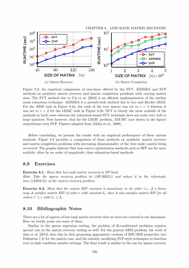
CHAPTER 8. LOW-RANK MATRIX RECOVERYR
UN
TIM
E (
se
c) SVT
SVP
SIZE OF MATRIX
(a) Matrix Recovery
SIZE OF MATRIX
RU
NT
IME
(se
c)
SVT
ADMiRA
SVP
(b) Matrix Completion
Figure 8.2: An empirical comparison of run-times offered by the SVT, ADMiRA and SVPmethods on synthetic matrix recovery and matrix completion problems with varying matrixsizes. The SVT method due to Cai et al. [2010] is an efficient implementation of the nuclearnorm relaxation technique. ADMiRA is a pursuit-style method due to Lee and Bresler [2010].For the ARM task in Figure 8.2a, the rank of the true matrix was set to r = 5 whereas itwas set to r = 2 for the LRMC task in Figure 8.2b. SVT is clearly the most scalable of themethods in both cases whereas the relaxation-based SVT technique does not scale very well tolarge matrices. Note however, that for the LRMC problem, AM-MC (not shown in the figure)outperforms even SVP. Figures adapted from [Meka et al., 2008].
Before concluding, we present the reader with an empirical performance of these variousmethods. Figure 8.2 provides a comparison of these methods on synthetic matrix recoveryand matrix completion problems with increasing dimensionality of the (low-rank) matrix beingrecovered. The graphs indicate that non-convex optimization methods such as IHT are far morescalable, often by an order of magnitude, than relaxation-based methods.
8.9 Exercises
Exercise 8.1. Show that low-rank matrix recovery is NP-hard.Hint: Take the sparse recovery problem in ((SP-REG)) and reduce it to the reformula-tion ((ARM-2)) of the matrix recovery problem.
Exercise 8.2. Show that the matrix RIP constant is monotonic in its order i.e., if a linearmap A satisfies matrix RIP of order r with constant δr, then it also satisfies matrix RIP for allorders r′ ≤ r with δr′ ≤ δr.
8.10 Bibliographic Notes
There are a lot of aspects of low-rank matrix recovery that we have not covered in our discussion.Here we briefly point out some of these.
Similar to the sparse regression setting, the problem of ill-conditioned problems requiresspecial care in the matrix recovery setting as well. For the general ARM problem, the work ofJain et al. [2014] does this by first proposing appropriate versions of RSC-RSS properties (seeDefinition 7.4) for the matrix case, and the suitably modifying SVP-style techniques to functioneven in high condition number settings. The final result is similar to the one for sparse recovery
106
8.10. BIBLIOGRAPHIC NOTES(see Theorem 7.4) wherein a more “relaxed” projection step is required by using a rank q > rwhile executing the SVP algorithm.
It turns out to be challenging to prove convergence results for SVP for the LRMC problem.This is primarily due to the difficulty in establishing the matrix RIP property for the affinetransformation used in the problem. The affine map simply selects a few elements of the matrixand reproduces them which makes establishing RIP properties harder in this setting. Specifically,even though the initialization step can be shown to yield a matrix that satisfies matrix RIP[Jain et al., 2010], if the underlying matrix is low-rank and incoherent, it becomes challengingto show that RIP-ness is maintained across iterates. Jain and Netrapalli [2015] overcome thisby executing the SVP algorithm in a stage-wise fashion which resembles ADMiRA-like pursuitapproaches.
Several works have furthered the alternating minimization approach itself by reducing itssample complexity [Hardt, 2014], giving recovery guarantees independent of the condition num-ber of the problem [Hardt and Wootters, 2014, Jain and Netrapalli, 2015], designing universalsampling schemes for recovery [Bhojanapalli and Jain, 2014], as well as tackling settings wheresome of the revealed entries of the matrix may be corrupted [Chen et al., 2016, Cherapanamjeriet al., 2017].
Another interesting line of work for matrix completion is that of [Ge et al., 2016, Sun andLu, 2015] which shows that under certain regularization assumptions, the matrix completionproblem does not have any non-optimal stationary points once one gets close-enough to theglobal minimum. Thus, one can use any method for convex optimization such as alternatingminimization, gradient descent, stochastic gradient descent, and its variants we studied in § 6,once one is close enough to the global minimum.
107
The official publication is available from now publishers viahttp://dx.doi.org/10.1561/2200000058
Chapter 9
Robust Linear Regression
In this section, we will look at the problem of robust linear regression. Simply put, it is the taskof performing linear regression in the presence of adversarial outliers or corruptions. Let us takea look at some motivating applications.
9.1 Motivating Applications
The problem of regression has widespread application in signal processing, financial andeconomic analysis, as well as machine learning and data analytics. In most real life applications,the data presented to the algorithm has some amount of noise in it. However, at times, datamay be riddled with missing values and corruptions, and that too of a malicious nature. Itis useful to design algorithms that can assure stable operation even in the presence of suchcorruptions.
Face Recognition The task of face recognition is widely useful in areas such as biometrics andautomated image annotation. In biometrics, a fundamental problem is to identify if a new faceimage belongs to that of a registered individual or not. This problem can be cast as a regressionproblem by trying to fit various features of the new image to corresponding features of existingimages of the individual in the registered database. More specifically, assume that images arerepresented as n-dimensional feature vectors say, using simple pixel-based features. Also assumethat there already exist p images of the person in the database.
Our task is to represent the new image xt ∈ Rn in terms of the database images X =[x1, . . . ,xp] ∈ Rn×p of that person. A nice way to do this is to perform a linear interpolation asfollows
minw∈Rp
∥∥∥xt −Xw∥∥∥2
2=
n∑i=1
(xti −Xiw)2.
If the person is genuine, then there will exist a combination w∗ such that for all i, we havexti ≈ Xiw∗ i.e., all features can be faithfully reconstructed. Thus, the fit will be nice and wewill admit the person. However, the same becomes problematic if the new image has occlusions.For example, if the person is genuine but wearing a pair of sunglasses or sporting a beard. Insuch cases, some of the pixels xti will appear corrupted, cause us to get a poor fit, and result ina false alarm. More specifically
xti = Xiw∗ + b∗iwhere b∗i = 0 on uncorrupted pixels but can take abnormally large and unpredictable valuesfor corrupted pixels, such as those corresponding to the sunglasses. Being able to still correctlyidentify the person involves computing the least squares fit in the presence of such corruptions.
108
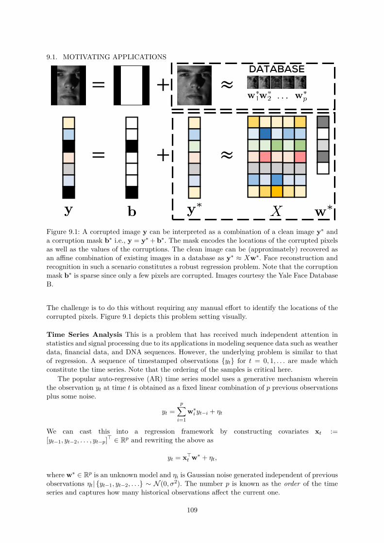
9.1. MOTIVATING APPLICATIONS
=
= ≈
+
+
DATABASE
≈
Figure 9.1: A corrupted image y can be interpreted as a combination of a clean image y∗ anda corruption mask b∗ i.e., y = y∗ + b∗. The mask encodes the locations of the corrupted pixelsas well as the values of the corruptions. The clean image can be (approximately) recovered asan affine combination of existing images in a database as y∗ ≈ Xw∗. Face reconstruction andrecognition in such a scenario constitutes a robust regression problem. Note that the corruptionmask b∗ is sparse since only a few pixels are corrupted. Images courtesy the Yale Face DatabaseB.
The challenge is to do this without requiring any manual effort to identify the locations of thecorrupted pixels. Figure 9.1 depicts this problem setting visually.
Time Series Analysis This is a problem that has received much independent attention instatistics and signal processing due to its applications in modeling sequence data such as weatherdata, financial data, and DNA sequences. However, the underlying problem is similar to thatof regression. A sequence of timestamped observations yt for t = 0, 1, . . . are made whichconstitute the time series. Note that the ordering of the samples is critical here.
The popular auto-regressive (AR) time series model uses a generative mechanism whereinthe observation yt at time t is obtained as a fixed linear combination of p previous observationsplus some noise.
yt =p∑i=1
w∗i yt−i + ηt
We can cast this into a regression framework by constructing covariates xt :=[yt−1, yt−2, . . . , yt−p]> ∈ Rp and rewriting the above as
yt = x>t w∗ + ηt,
where w∗ ∈ Rp is an unknown model and ηi is Gaussian noise generated independent of previousobservations ηt| yt−1, yt−2, . . . ∼ N (0, σ2). The number p is known as the order of the timeseries and captures how many historical observations affect the current one.
109

CHAPTER 9. ROBUST LINEAR REGRESSIONIs not uncommon to encounter situations where the time series experiences gross corruptions.
Examples may include observation or sensing errors or unmodeled factors such as dips andupheavals in stock prices due to political or socio-economic events. Thus, we have
yt = x>t w∗ + ηt + b∗twhere b∗t can take unpredictable values for corrupted time instances and 0 otherwise. In timeseries literature, two corruption models are popular. In the additive model, observations at timesteps subsequent to a corruption are constructed using the uncorrupted values i.e., b∗t does notinfluence the values yτ for τ > t. Of course, observers may detect the corruption at time t butthe underlying time series goes on as though nothing happened.
However, in the innovative model, observations at time instances subsequent to a corruptionuse the corrupted value i.e., b∗t is involved in constructing the values yτ for τ = t+ 1, . . . , t+ p.Innovative corruptions are simpler to handle as although the observation at the moment ofthe corruption i.e., yt, appears to deviate from that predicted by the base model i.e., x>t w∗,subsequent observations fall in line with the predictions once more (unless there are morecorruptions down the line). In the additive model however, observations can seem to deviatefrom the predictions of the base model for several iterations. In particular, yτ can disagree withx>τ w∗ for times τ = t, t+ 1, . . . , t+ p, even if there is only a single corruption at time t.
A time series analysis technique which seeks to study the “usual” behavior of the modelinvolved, such as stock prices, might wish to exclude such aberrations, whether additive orinnovative. However it is unreasonable, as well as error prone, to expect manual exclusion ofsuch corruptions which motivates the problem of robust time series analysis. Note that timeseries analysis is a more challenging problem than regression since the “covariates” in this casext,xt+1, . . . are heavily correlated with each other as they share a large number of coordinateswhereas in regression they are usually assumed to be independent.
9.2 Problem FormulationLet us recall the regression model studied in § 5.1 and § 7.2. In a linear regression setting,responses are modeled as a (possibly sparse) linear function of the data features to which someadditive noise is added, i.e., we have
yi = x>i w∗ + ηi.
However, notice that in previous discussions, we termed the noise as benign, and even found itappropriate to assume it could be modeled as a Gaussian random variable. This is usually ac-ceptable when the noise is expected to be non-deliberate or the result of small and unstructuredperturbations. However, the outliers or corruptions in the examples that we just saw, seem todefy these assumptions.
In the face recognition case, salt and pepper noise due to sensor disturbances, or lightingchanges can be considered benign noise. However, it is improper to consider structured occlusionssuch as sunglasses or beards as benign as some of them may even be a part of a maliciousattempt to fool the system. Even in the time series analysis setting, there might be maliciousforces at play in the stock market which cause stock prices to significantly deviate from theirusual variations and trends.
Such corruptions can severely disrupt the modeling process and hamper our understandingof the system. To handle them, we will need a more refined model that distinguishes betweenbenign and unstructured errors, and errors that are deliberate, malicious and structured. Therobust regression model best describes this problem setting
yi = x>i w∗ + ηi + b∗i
110
9.3. ROBUST REGRESSION VIA ALTERNATING MINIMIZATIONAlgorithm 11 AltMin for Robust Regression (AM-RR)Input: Data X,y, number of corruptions kOutput: An accurate model w ∈ Rp1: w1 ← 0, S1 = [1 : n− k]2: for t = 1, 2, . . . do3: wt+1 ← arg minw∈Rp
∑i∈St(yi − x>i w)2
4: St+1 ← arg min|S|=n−k∑i∈S(yi − x>i wt+1)2
5: end for6: return wt
where the variable b∗i encodes the additional corruption introduced into the response. Our goalis to take a set of n (possibly) corrupted data points (xi, yi)ni=1 and recover the underlyingparameter vector w∗, i.e.,
minw∈Rp,b∈Rn‖b‖0≤k
‖y−Xw− b‖22 , (ROB-REG)
The variables b∗i can be unbounded in magnitude and of arbitrary sign. However, we assumethat only a few data points are corrupted i.e., the vector b∗ = [b∗1,b∗2, . . . ,b∗n] is sparse ‖b∗‖0 ≤k. Indeed it is impossible1 to recover the model w∗ if more than half the points are corruptedi.e., k ≥ n/2. A worthy goal is to develop algorithms that can tolerate as large a value of k aspossible. We will study how two non-convex optimization techniques, namely gAM and gPGD,can be used to solve this problem. We point to other approaches, as well as extensions such asrobust sparse recovery, in the bibliographic notes.
9.3 Robust Regression via Alternating Minimization
The key to applying alternating minimization to the robust regression problem is to identifythe two critical parameters in this problem. Let us assume that there is no Gaussian noise inthe model i.e., y = Xw∗ + b∗ where b∗ is k-sparse but can contain unbounded entries in itssupport.
It can be seen that w∗ and supp(b∗) =: S∗, i.e., the true model and the locations of theuncorrupted points, are the two most crucial elements since given one, finding the other is verysimple. Indeed, if someone were to magically hand us w∗, it is trivial to identify S∗ by simplyidentifying data points where yi = x>i w∗. On the other hand, given S∗, it is simple to obtainw∗ by simply solving a least squares regression problem on the set of data points in the set S∗.Thus we can rewrite the robust regression problem as
minw∈Rp|S|=n−k
∥∥∥yS −XSw∥∥∥2
2(ROB-REG-2)
This gives us a direct way of applying the gAM approach to this problem as outlined in theAM-RR algorithm (Algorithm 11). The work of Bhatia et al. [2015] showed that this techniqueand its variants offer scalable solutions to the robust regression problem.
In order to execute the gAM protocol, AM-RR maintains a model estimate wt and an activeset St ⊂ [n] of points that are deemed clean at the moment. At every time step, true to thegAM philosophy, AM-RR first fixes the active set and updates the model, and then fixes themodel and updates the active set. The first step turns out to be nothing but least squares over
1See Exercise 9.1.
111
CHAPTER 9. ROBUST LINEAR REGRESSIONthe active set. For the second step, it is easy to see that the optimal solution is achieved simplyby taking the n− k data points with the smallest residuals (by magnitude) with respect to theupdated model and designating them to be the active set.
9.4 A Robust Recovery Guarantee for AM-RRTo simplify the analysis, we will assume that there is no Gaussian noise in the model i.e.,y = Xw∗ + b∗ where b∗ is k-sparse. To present the analysis of the AM-RR algorithm, we willneed the notions of subset strong convexity and smoothness.
Definition 9.1 (Subset Strong Convexity/Smoothness Property [Bhatia et al., 2015]). A matrixX ∈ Rn×p is said to satisfy the αk-subset strong convexity (SSC) property and the βk-subsetsmoothness property (SSS) of order k if for all sets S ⊂ [n] of size |S| ≤ k, we have, for allv ∈ Rp,
αk · ‖v‖22 ≤∥∥∥XSv
∥∥∥2
2≤ βk · ‖v‖22.
The SSC/SSS properties require that the design matrix formed by taking any subset of kpoints from the data set of n points act as an approximate isometry on all p dimensional points.These properties are related to the traditional RSC/RSS properties and it can be shown (seefor example, [Bhatia et al., 2015]) that RIP-inducing distributions over matrices (see § 7.6)also produce matrices that satisfy the SSC/SSS properties, with high probability. However, itis interesting to note that whereas the RIP definition is concerned with column subsets of thedesign matrix, SSC/SSS concerns itself with row subsets.
The nature of the SSC/SSS properties is readily seen to be very appropriate for AM-RR tosucceed. Since the algorithm uses only a subset of data points to estimate the model vector, itis essential that smaller subsets of data points of size n − k (in particular the true subset ofclean points S∗) also allow the model to be recovered. This is equivalent2 to requiring that thedesign matrices formed by smaller subsets of data points not identify distinct model vectors.This is exactly what the SSC property demands.
Given this, we can prove the following convergence guarantee for the AM-RR algorithm. Thereader would notice that the algorithm, despite being a gAM-style algorithm, does not requireprecise and careful initialization of the model and active set. This is in stark contrast to othergAM-style approaches we have seen so far, namely EM and AM-MC, both of which demandedcareful initialization.
Theorem 9.1. Let X ∈ Rn×p satisfy the SSC property at order n − k with parameter αn−kand the SSS property at order k with parameter βk such that βk/αn−k < 1√
2+1 . Let w∗ ∈ Rp
be an arbitrary model vector and y = Xw∗ + b∗ where ‖b∗‖0 ≤ k is a sparse vector of possiblyunbounded corruptions. Then AM-RR yields an ε-accurate solution
∥∥wt −w∗∥∥
2 ≤ ε in no morethan O
(log ‖b
∗‖2ε
)steps.
Proof. Let rt = y−Xwt denote the vector of residuals at time t and let Ct = (XSt)>XSt andS∗ = supp(b∗). Then the model update step of AM-RR solves a least squares problem ensuring
wt+1 = C−1t (XSt)>ySt
= C−1t (XSt)>(XStw∗ + b∗St)
= w∗ + C−1t (XSt)>b∗St .
2See Exercise 9.2.
112
9.4. A ROBUST RECOVERY GUARANTEE FOR AM-RRThe residuals with respect to this new model can be computed as
rt+1 = y−Xwt+1 = b∗ +XC−1t (XSt)>b∗St .
However, the active-set update step selects the set with smallest residuals, in particular, ensuringthat ∥∥∥rt+1
St+1
∥∥∥2
2≤∥∥∥rt+1S∗
∥∥∥2
2.
Plugging in the expression for rt+1 into both sides of the equation, using b∗S∗ = 0 and the factthat that for any matrix X and vector v we have∥∥∥XSv
∥∥∥2
2−∥∥∥XTv
∥∥∥2
2=∥∥∥XS\Tv
∥∥∥2
2−∥∥∥XT\Sv
∥∥∥2
2≤∥∥∥XS\Tv
∥∥∥2
2,
gives us, upon some simplification,∥∥∥b∗St+1
∥∥∥2
2≤∥∥∥XS∗\St+1C−1
t (XSt)>b∗St∥∥∥2
2
− 2(b∗St+1)>XSt+1C−1t (XSt)>b∗St
≤ β2k
α2n−k
∥∥b∗St∥∥22 + 2 · βk
αn−k·∥∥∥b∗St+1
∥∥∥2·∥∥b∗St∥∥2 ,
where the last step follows from an application of the SSC/SSS properties by noticing that|S∗\St+1| ≤ k and that b∗St and b∗St+1
are all k-sparse vectors since b∗ itself is a k-sparse vector.Solving the above equation gives us∥∥∥b∗St+1
∥∥∥2≤ (√
2 + 1) · βkαn−k
·∥∥b∗St∥∥2
The above result proves that in t = O(log ‖b
∗‖2ε
)iterations, the alternating minimization
procedure will identify an active set St such that∥∥∥b∗St∥∥∥2
≤ ε. It is easy3 to see that a leastsquares step on this active set will yield a model w satisfying∥∥∥wt −w∗
∥∥∥2
=∥∥∥C−1
t (XSt)>b∗St∥∥∥
2≤ βkαn−k
· ε ≤ ε,
since βk/αn−k < 1. This concludes the convergence guarantee.
The crucial assumption in the previous result is the requirement βk/αn−k < 1√2+1 . Clearly,
as k → 0, we have βk → 0 but if the matrix X is well conditioned we still have αn−k > 0. Thus,for small enough k, it is assured that we will have βk/αn−k < 1√
2+1 . The point at which thisoccurs is the so-called breakdown point of the algorithm – it is the largest number k such thatthe algorithm can tolerate k possibly adversarial corruptions and yet guarantee recovery.
Note that the quantity κk = βk/αn−k acts as the effective condition number of the problem.It plays the same role as the condition number did in the analysis of the gPGD and IHTalgorithms. It can be shown that for RIP-inducing distributions (see [Bhatia et al., 2015]),AM-RR can tolerate k = Ω(n) corruptions.
For the specific case of the design matrix being generated from a Gaussian distribution, itcan be shown that we have αn−k = Ω (n− k) and βk = O (k). This in turn can be used toshow that we have βk/αn−k < 1√
2+1 whenever k ≤ n/70. This means that AM-RR can tolerateup to n/70 corruptions when the design matrix is Gaussian. This indicates a high degree ofrobustness in the algorithm since these corruptions can be completely adversarial in terms oftheir location, as well as their magnitude. Note that AM-RR is able to ensure this withoutrequiring any specific initialization.
3See Exercise 9.3.
113
CHAPTER 9. ROBUST LINEAR REGRESSION9.5 Alternating Minimization via Gradient Updates
Similar to the gradient-based EM heuristic we looked at in § 5.5, we can make the alternatingminimization process in AM-RR much cheaper by executing a gradient step for the alternations.More specifically, we can execute step 3 of AM-RR as
wt+1 ← wt − η ·∑i∈St
(x>i w− yi)xi,
for some step size parameter η. It can be shown (see [Bhatia et al., 2015]) that this processenjoys the same linear rate of convergence as AM-RR. However, notice that both alternations(model update as well as active set update) in this gradient-descent version can be carried outin (near-)linear time. This is in contrast with AM-RR which takes super-quadratic time in eachalternation to discover the least squares solution. In practice, this makes the gradient versionmuch faster (often by an order of magnitude) as compared to the fully corrective version.
However, once we have obtained a reasonably good estimate of S∗, it is better to executethe least squares solution to obtain the final solution in a single stroke. Thus, the gradient andfully corrective steps can be mixed together to great effect. In practice, such hybrid techniquesoffer the fastest convergence. We refer the reader to § 9.7 for a brief discussion on this and to[Bhatia et al., 2015] for details.
9.6 Robust Regression via Projected Gradient Descent
It is possible to devise an alternate formulation for the robust regression problem that allowsus to apply the gPGD technique instead. The work of [Bhatia et al., 2017] uses this alternateformulation to arrive at a solution that enjoys consistency properties. Note that if someone gaveus a good estimate b of the corruption vector, we could use it to clean up the responses as y− b,and re-estimate the model as
w(b) = arg minw∈Rp
∥∥∥(y− b)−Xw∥∥∥2
2= (X>X)−1X>(y− b).
The residuals corresponding to this new model estimate would be∥∥∥y− b−X · w(b)∥∥∥2
2=∥∥∥(I − PX)(y− b)
∥∥∥2
2,
where PX = X(X>X)−1X>. The above calculation shows that an equivalent formulation forthe robust regression problem ((ROB-REG)) is the following
min‖b‖0=k
‖(I − PX)(y− b)‖22 ,
to which we can apply gPGD (Algorithm 2) since it now resembles a sparse recovery problem!This problem enjoys4 the restricted isometry property whenever the design matrix X is sampledfrom an RIP-inducing distribution (see § 7.6). This shows that an application of the gPGDtechnique will guarantee recovery of the optimal corruption vector b∗ at a linear rate. Once wehave an ε-optimal estimate b of b∗, a good model w can be found by solving the least squaresproblem.
w(b) = (X>X)−1X>(y− b),4See Exercise 9.4.
114

9.7. EMPIRICAL COMPARISONR
UN
TIM
E (
se
c) Ex. LASSO
AM-RR
gPGD
DATASET SIZE
(a) Run-time Comparison
RUNTIME (sec)
DALM
AM-RR
AM-RR-Hyb
AM-RR-GD
(b) Convergence Comparison
Figure 9.2: An empirical comparison of the performance offered by various approaches for robustregression. Figure 9.2a (adapted from [Bhatia et al., 2017]) compares Extended LASSO, a state-of-the-art relaxation method by Nguyen and Tran [2013b], AM-RR and the gPGD method from§ 9.6 on a robust regression problem in p = 1000 dimensions with 30% data points corrupted.Non-convex techniques such as AM-RR and gPGD are more than an order of magnitude faster,and scale much better, than Extended LASSO. Figure 9.2b (adapted from [Bhatia et al., 2015])compares various solvers on a robust regression problem in p = 300 dimensions with 1800data points of which 40% are corrupted. The solvers include the gAM-style solver AM-RR,a variant using gradient-based updates, a hybrid method (see § 9.5), and the DALM method[Yang et al., 2013], a state-of-the-art solver for relaxed LASSO-style formulations. The hybridmethod is the fastest of all the techniques. In general, all AM-RR variants are much faster thanthe relaxation-based method.
as before. It is a simple exercise to show that if∥∥∥b− b∗
∥∥∥2≤ ε, then
∥∥∥w(b)−w∗∥∥∥ ≤ O( ε
α
),
where α is the RSC parameter of the problem. Note that this shows how the gPGD techniquecan be applied to perform recovery not only when the parameter is sparse in the model domain(for instance in the gene expression analysis problem), but also when the parameter is sparsein the data domain, as in the robust regression example.
9.7 Empirical Comparison
Before concluding, we present some discussion on the empirical performance of various algo-rithms on the robust regression problem. Figure 9.2a compares the running times of variousrobust regression approaches on synthetic problems as the number of data points available inthe dataset increases. Similar trends are seen if the data dimensionality increases. The graphshows that non-convex techniques such as AM-RR and gPGD offer much more scalable solu-tions than relaxation-based methods. Figure 9.2b similarly demonstrates how variants of thebasic AM-RR procedure can offer significantly faster convergence. Figure 9.3 looks at a realis-tic example of face reconstruction under occlusions and demonstrates how AM-RR is able tosuccessfully recover the face image even when significant portions of the face are occluded.
115
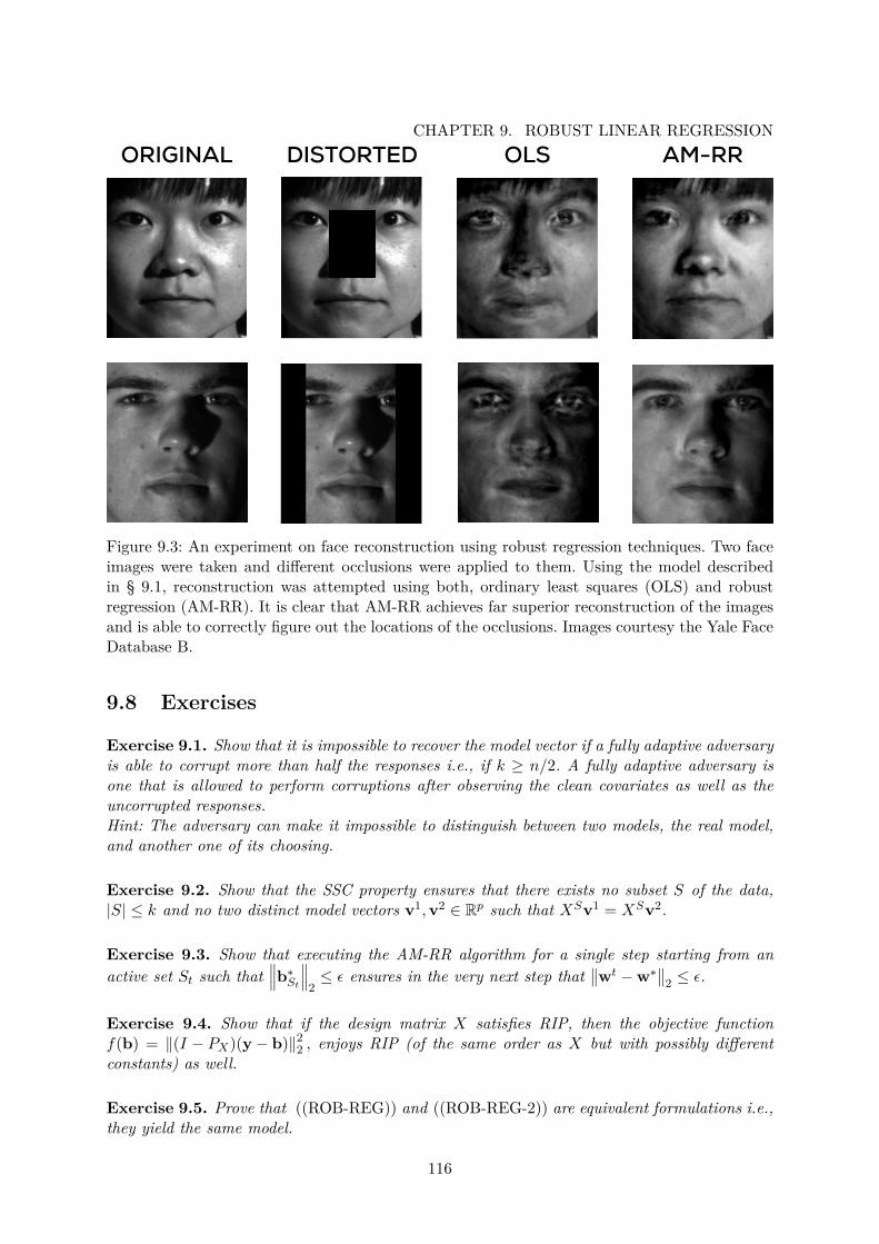
CHAPTER 9. ROBUST LINEAR REGRESSIONORIGINAL DISTORTED OLS AM-RR
Figure 9.3: An experiment on face reconstruction using robust regression techniques. Two faceimages were taken and different occlusions were applied to them. Using the model describedin § 9.1, reconstruction was attempted using both, ordinary least squares (OLS) and robustregression (AM-RR). It is clear that AM-RR achieves far superior reconstruction of the imagesand is able to correctly figure out the locations of the occlusions. Images courtesy the Yale FaceDatabase B.
9.8 Exercises
Exercise 9.1. Show that it is impossible to recover the model vector if a fully adaptive adversaryis able to corrupt more than half the responses i.e., if k ≥ n/2. A fully adaptive adversary isone that is allowed to perform corruptions after observing the clean covariates as well as theuncorrupted responses.Hint: The adversary can make it impossible to distinguish between two models, the real model,and another one of its choosing.
Exercise 9.2. Show that the SSC property ensures that there exists no subset S of the data,|S| ≤ k and no two distinct model vectors v1,v2 ∈ Rp such that XSv1 = XSv2.
Exercise 9.3. Show that executing the AM-RR algorithm for a single step starting from anactive set St such that
∥∥∥b∗St∥∥∥2≤ ε ensures in the very next step that
∥∥wt −w∗∥∥
2 ≤ ε.
Exercise 9.4. Show that if the design matrix X satisfies RIP, then the objective functionf(b) = ‖(I − PX)(y− b)‖22 , enjoys RIP (of the same order as X but with possibly differentconstants) as well.
Exercise 9.5. Prove that ((ROB-REG)) and ((ROB-REG-2)) are equivalent formulations i.e.,they yield the same model.
116
9.9. BIBLIOGRAPHIC NOTES9.9 Bibliographic NotesThe problem of robust estimation has been well studied in the statistics community. Indeed,there exist entire texts devoted to this area [Rousseeuw and Leroy, 1987, Maronna et al., 2006]which look at robust estimators for regression and other problems. However, these methods ofteninvolve estimators, such as the least median of squares estimator, that have an exponential timecomplexity.
It is notable that these infeasible estimators often have attractive theoretical properties suchas a high breakdown point. For instance, the work of Rousseeuw [1984] shows that the leastmedian of squares method enjoys a breakdown point of as high as n/2− p. In contrast, AM-RRis only able to handle n/70 errors. However, whereas the gradient descent version of AM-RR canbe executed in near-linear time, the least median of squares method requires time exponentialin p.
There have been relaxation based approaches to solving robust regression and time seriesproblems as well. Chief of them include the works of Chen and Dalalyan [2012], Chen et al.[2013] which look at the Dantzig selector methods and the trimmed product techniques toperform estimation, and the works of Wright et al. [2009], Nguyen and Tran [2013a]. The workof Chen et al. [2013] considers corruptions not only in the responses, but in the covariates aswell. However, these methods tend to scale poorly to really large scale problems owing to thenon-smooth nature of the optimization problems that they end up solving. The non-convexoptimization techniques we have studied, on the other hand, require linear time or else haveclosed-form updates.
Recent years have seen the application of non-convex techniques to robust estimation. How-ever these works can be traced back to the classical work of Fischler and Bolles [1981] thatdeveloped the RANSAC algorithm that is very widely used in fields such as computer vision.The RANSAC algorithm samples multiple candidate active sets and returns the least squaresestimate on the set with least residual error.
Although the RANSAC method does not enjoy strong theoretical guarantees in the faceof an adaptive adversary and a large number of corruptions, the method is seen to work wellwhen there are very few outliers. Later works, such as that of She and Owen [2011] appliedsoft-thresholding techniques to the problem followed by the work of Bhatia et al. [2015] whichapplied the alternating minimization algorithm we studied here. Bhatia et al. [2015] also lookedat the problem of robust sparse recovery.
The time series literature has also seen the application of various techniques for robustestimation including robust M-estimators in both the additive and innovative outlier models[Martin and Zeh, 1978, Stockinger and Dutter, 1987] and least trimmed squares [Croux andJoossens, 2008].
117
The official publication is available from now publishers viahttp://dx.doi.org/10.1561/2200000058
Chapter 10
Phase Retrieval
In this section, we will take a look at the phase retrieval problem, a non-convex optimizationproblem with applications in several domains. We briefly mentioned this problem in § 5 whenwe were discussing mixed regression. At a high level, phase retrieval is equivalent to discov-ering a complex signal using observations that reveal only the magnitudes of (complex) linearmeasurements over that signal. The phases of the measurements are not revealed to us.
Over reals, this reduces to solving a system of quadratic equations which is known to becomputationally intractable to solve exactly. Fortunately however, typical phase retrieval sys-tems usually require solving quadratic systems that have nice randomized structures in thecoefficients of the quadratic equations. These structures can be exploited to efficiently solvethese systems. In this section we will look at various algorithms that achieve this.
10.1 Motivating Applications
The problem of phase retrieval arises in areas of signal processing where the phase of a signalbeing measured is irrevocably lost, or at best, unreliably obtained. The recovery of the signalin such situations becomes closely linked to our ability to perform phase retrieval.
X-ray Crystallography The goal in X-ray crystallography is to find the structure of a smallmolecule by bombarding it with X-rays from various angles and measuring the trajectories andintensities of the diffracted photons on a film. These quantities can be used to glean the inter-nal three-dimensional structure of the electron cloud within the crystal, revealing the atomicarrangements therein. This technique has been found to be immensely useful in imaging speci-mens with a crystalline structure and has been historically significant in revealing the interiorcomposition of several compounds, both inorganic and organic.
A notable example is that of nucleic acids such as DNA whose structure was revealed inthe seminal work of Franklin and Gosling [1953a] which immediately led Francis and Crick topropose its double helix structure. The reader may be intrigued by the now famous Photo 51which provided critical support to the helical structure-theory of DNA [Franklin and Gosling,1953b]. We refer the reader to the expository work of Lucas [2008] for a technical and historicalaccount of how these discoveries came to be.
Transmission Electron Microscopy (TEM) This technique uses a focused beam ofelectrons instead of high energy photons to image the object of study. This technique worksbest with ultra thin specimens which do not absorb electrons but let the beam of electrons passthrough. The electrons interact with the atomic structure of the specimen and are captured atthe other end using a sensing mechanism. TEM is capable of resolutions far higher than those
118
10.2. PROBLEM FORMULATIONpossible using photonic imaging techniques due to the extremely small de-Broglie wavelengthof electrons.
Coherent Diffraction Imaging (CDI) This is a widely used technique for studying nanos-tructures such as nanotubes, nanocrystals and the like. A highly coherent beam of X-rays ismade incident on the object of study and the diffracted rays allowed to interfere to produce adiffraction pattern which is used to recover the structure of the object. A key differentiatingfactor in CDI is the absence of any lenses to focus light onto the specimen, as opposed to othermethods such as TEM/X-Ray crystallography which use optical or electromagnetic lenses tofocus the incident beam and then refocus the diffracted beam. The absence of any lenses inCDI is very advantageous since it results in aberration-free patterns. Moreover, this way theresolution of the technique is only dependent on the wavelength and other properties of theincident rays rather than the material of the lens etc.
10.2 Problem Formulation
Bombarding a structure with X-rays or other beams can be shown to be equivalent to takingrandom Fourier measurements of its internal structure. More specifically, let w∗ ∈ Cp denotethe vector that represents the density of electrons throughout the crystal, signifying its internalstructure. Then, under simplifying regularity assumptions such as perfect periodicity, X-raycrystallography can be modeled as transforming w∗ into y = Xw∗ ∈ Cn where X ∈ Cn×p haseach of its rows sampled from a Fourier measurement matrix, i.e,Xab = exp
(−2π(a−1)(b−1)
p
), b =
1, . . . , p for some random a ∈ [p].Unfortunately, the measurements made by the sensors in the above applications are not able
to observe the Fourier measurements exactly. Instead of observing complex valued transforma-tions yk ∈ C of the signal y, all we observe are the real value magnitudes |yk| ∈ R, the phasebeing lost in the signal acquisition process. A natural question arises whether it is still possibleto recover w∗ or not.
Note that if the signal and the measurement matrices are real then |yk|2 = (x>k w∗)2. Thus,the goal is simply to recover a model w by solving a system of n quadratic equations describedabove. Although problem of solving a system of quadratic equations is intractable in general,in the special case of phase retrieval, it is possible to exploit the fact that the vectors xk aresampled randomly, to develop recovery algorithms that are efficient, as well as require only asmall number n of measurements.
We note that the state of the art in phase retrieval literature is yet unable to guaranteerecovery from random Fourier measurements, which closely model situations arising in crystal-lography and other imaging applications. Current analyses mostly consider the case when thesensing matrix X has random Gaussian entries. A notable exception to the above is the workof Candès et al. [2015] which is able to address coded diffraction measurements. These are morerelevant to what is used in practice but still complicated to design. For sake of simplicity, we willonly focus on the Gaussian measurement case in our discussions. This would allow us to studythe algorithmic techniques used to solve the problem without getting involved in the intricaciesof Fourier or coded diffraction measurements.
To formalize our problem statement, we let w∗ ∈ Cp be an unknown p-dimensional signal,X = [x1,x2, . . . ,xn]> ∈ Cn×p be a measurement matrix. Our goal is to recover w∗ given X
and |y|, where y = [y1, y2, . . . , yk]> ∈ Cn = Xw∗ and |yk| =∣∣∣x>i w∗
∣∣∣. Our focus would be on
the special case where Xkji.i.d.∼ N (0, 1) + i · N (0, 1) where i2 = −1. We would like to recover
w∗ efficiently using only n = O (p) measurements. We will study how gAM and gPGD-style
119
CHAPTER 10. PHASE RETRIEVALAlgorithm 12 Gerchberg-Saxton Alternating Minimization (GSAM)Input: Measurement matrix X ∈ Cn×p, observed response magnitudes |y| ∈ Rn+, desired accu-
racy εOutput: A signal w ∈ Cp1: Set T ← log 1/ε2: Partition n data points into T + 1 sets S0, S1, . . . , ST3: w0 ← eig
(1|S0|
∑k∈S0 |yk|
2 · xkx>k , 1)
//Leading eigenvector4: for t = 1, 2, . . . , T do5: Phase Estimation: φk = x>k wt−1/|x>k wt−1|, for all k ∈ St6: Signal Estimation: wt = arg minw∈Cp
∑k∈St ||yk| · φk − x>k w|2
7: end for8: return wT
techniques can be used to solve this problem. We will point to approaches using the relaxationtechnique in the bibliographic notes.
Notation: We will abuse the notation x> to denote the complex row-conjugate of a complexvector x ∈ Cp, something that is usually denoted by x∗. A random vector x = a + ib ∈ Cn willbe said to be distributed according to the standard Gaussian distribution over Cn, denoted asNC(0, I) if a,b ∈ Rn are independently distributed as standard (real valued) Gaussian vectorsi.e., a,b ∼ N (0, In).
10.3 Phase Retrieval via Alternating Minimization
One of the most popular approaches for solving the phase retrieval problem is a simple applica-tion of the gAM approach, first proposed by Gerchberg and Saxton [1972] more than 4 decadesago. The intuition behind the approach is routine – there exist two parameters of interest inthe problem – the phase of the data points i.e., yk/ |yk|, and the true signal w∗. Just as before,we observe a two-way connection between these parameters. Given the true phase values ofthe points φk = yk/|yk|, the signal w∗ can be recovered simply by solving a system of linearequations: φk · |yk| = x>k w, k = 1, . . . , n. On the other hand, given w∗, estimating the phase ofthe points is straightforward as φk = (x>k w∗)/|x>k w∗|.
Given the above, a gAM-style approach naturally arises: we alternately estimate φk and w∗.More precisely, at the t-th step, we first estimate φtk using wt−1 as φtk = (x>k wt−1)/|x>k wt−1| andthen update our estimate of w by solving a least squares problem wt = arg minw
∑k |φtk|yk| −
x>k w|2 over complex variables. Algorithm 12 presents the details of this Gerchberg-Saxton Al-ternating Minimization (GSAM) method. To avoid correlations, the algorithm performs thesealternations on distinct sets of points at each time step. These disjoint sets can be created bysub-sampling the overall available data.
In their original work, Gerchberg and Saxton [1972] proposed to use a random vector w0
for initialization. However, the recent work of Netrapalli et al. [2013] demonstrated that a morecareful initialization, in particular the largest eigenvector of M =
∑k |yk|2 · xkx>k , is beneficial.
Such a spectral initialization leads to an initial solution that is already at most a (small) constantdistance away from the optimal solution w∗.
As we have seen to be the case with most gAM-style approaches, including the EM algo-rithm, this approximately optimal initialization is crucial to allow the alternating minimizationprocedure to take over and push the iterates toward the globally optimal solution.
120
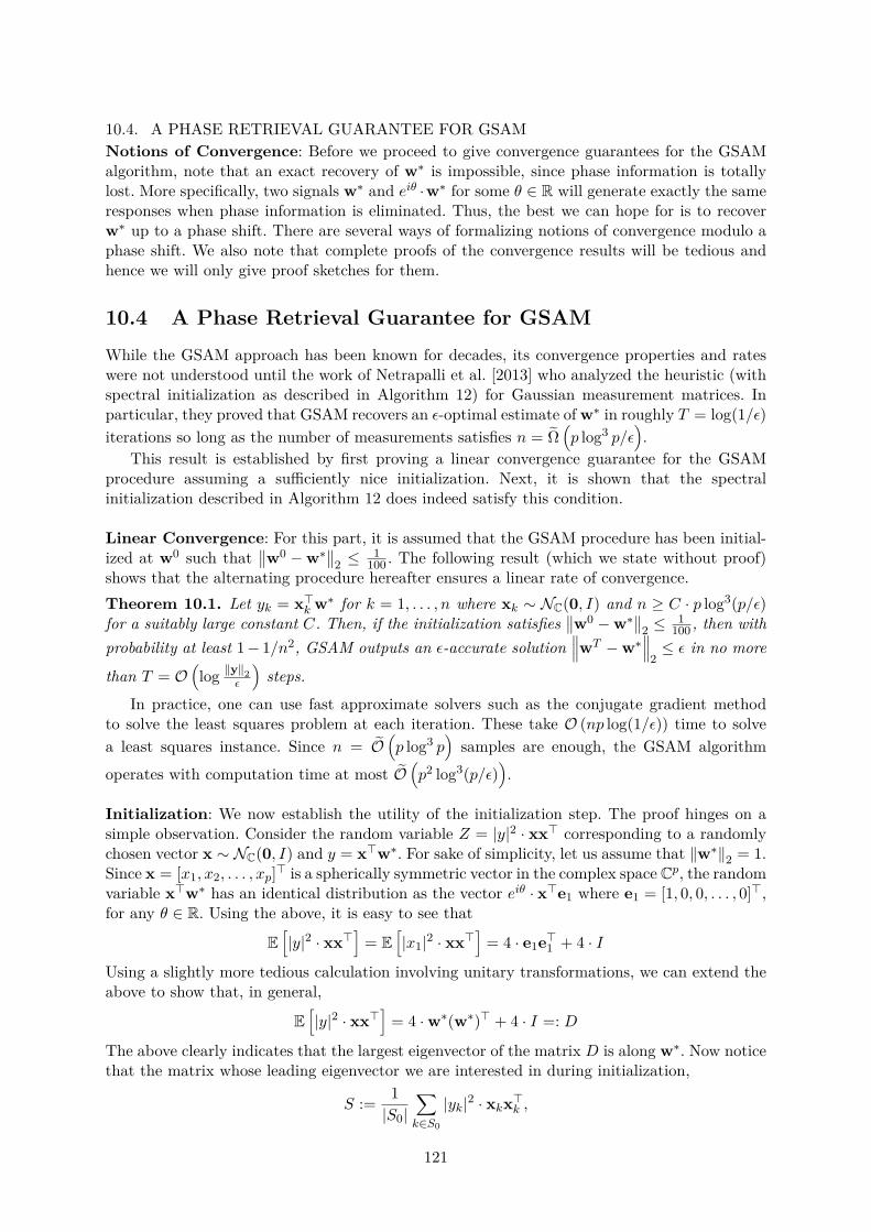
10.4. A PHASE RETRIEVAL GUARANTEE FOR GSAMNotions of Convergence: Before we proceed to give convergence guarantees for the GSAMalgorithm, note that an exact recovery of w∗ is impossible, since phase information is totallylost. More specifically, two signals w∗ and eiθ ·w∗ for some θ ∈ R will generate exactly the sameresponses when phase information is eliminated. Thus, the best we can hope for is to recoverw∗ up to a phase shift. There are several ways of formalizing notions of convergence modulo aphase shift. We also note that complete proofs of the convergence results will be tedious andhence we will only give proof sketches for them.
10.4 A Phase Retrieval Guarantee for GSAMWhile the GSAM approach has been known for decades, its convergence properties and rateswere not understood until the work of Netrapalli et al. [2013] who analyzed the heuristic (withspectral initialization as described in Algorithm 12) for Gaussian measurement matrices. Inparticular, they proved that GSAM recovers an ε-optimal estimate of w∗ in roughly T = log(1/ε)iterations so long as the number of measurements satisfies n = Ω
(p log3 p/ε
).
This result is established by first proving a linear convergence guarantee for the GSAMprocedure assuming a sufficiently nice initialization. Next, it is shown that the spectralinitialization described in Algorithm 12 does indeed satisfy this condition.
Linear Convergence: For this part, it is assumed that the GSAM procedure has been initial-ized at w0 such that
∥∥w0 −w∗∥∥
2 ≤1
100 . The following result (which we state without proof)shows that the alternating procedure hereafter ensures a linear rate of convergence.Theorem 10.1. Let yk = x>k w∗ for k = 1, . . . , n where xk ∼ NC(0, I) and n ≥ C · p log3(p/ε)for a suitably large constant C. Then, if the initialization satisfies
∥∥w0 −w∗∥∥
2 ≤1
100 , then withprobability at least 1− 1/n2, GSAM outputs an ε-accurate solution
∥∥∥wT −w∗∥∥∥
2≤ ε in no more
than T = O(log ‖y‖2
ε
)steps.
In practice, one can use fast approximate solvers such as the conjugate gradient methodto solve the least squares problem at each iteration. These take O (np log(1/ε)) time to solvea least squares instance. Since n = O
(p log3 p
)samples are enough, the GSAM algorithm
operates with computation time at most O(p2 log3(p/ε)
).
Initialization: We now establish the utility of the initialization step. The proof hinges on asimple observation. Consider the random variable Z = |y|2 · xx> corresponding to a randomlychosen vector x ∼ NC(0, I) and y = x>w∗. For sake of simplicity, let us assume that ‖w∗‖2 = 1.Since x = [x1, x2, . . . , xp]> is a spherically symmetric vector in the complex space Cp, the randomvariable x>w∗ has an identical distribution as the vector eiθ · x>e1 where e1 = [1, 0, 0, . . . , 0]>,for any θ ∈ R. Using the above, it is easy to see that
E[|y|2 · xx>
]= E
[|x1|2 · xx>
]= 4 · e1e>1 + 4 · I
Using a slightly more tedious calculation involving unitary transformations, we can extend theabove to show that, in general,
E[|y|2 · xx>
]= 4 ·w∗(w∗)> + 4 · I =: D
The above clearly indicates that the largest eigenvector of the matrix D is along w∗. Now noticethat the matrix whose leading eigenvector we are interested in during initialization,
S := 1|S0|
∑k∈S0
|yk|2 · xkx>k ,
121
CHAPTER 10. PHASE RETRIEVALis simply an empirical estimate to the expectation E
[|y|2 · xx>
]= D. Indeed, we have E [S] =
D. Thus, it is reasonable to expect that the leading eigenvector of S would also be aligned tow∗. We can make this statement precise using results from the concentration of finite sums ofself-adjoint independent random matrices from [Tropp, 2012].
Theorem 10.2. The spectral initialization method (Step 3 of Algorithm 12), with probabilityat least 1− 1/|S0|2 ≤ 1− 1/p2, ensures an initialization w0 such that
∥∥w0 −w∗∥∥
2 ≤ c for anyconstant c > 0, so long as it is executed with a randomly chosen set S0 of data points of size|S0| ≥ C · p log p for a suitably large constant C depending on c.
Proof. To make the analysis simple, we will continue to assume that w∗ = eiθ · e1 for someθ ∈ R. We can use Bernstein-style results for matrix concentration (for instance, see [Tropp,2012, Theorem 1.5]) to show that for any chosen constant c > 0, if n ≥ C · p log p for a largeenough constant C that depends on the constant c, then with probability at least 1 − 1/|S0|2,we have
‖S −D‖2 ≤ c
Note that the norm being used above is the spectral/operator norm on matrices. Given this, itis possible to get a handle on the leading eigenvalue of S. Observe that since w0 is the leadingeigenvector of S, and since we have assumed w∗ = eiθ · e1, we have∣∣⟨w0, Sw0⟩∣∣ ≥ |〈w∗, Sw∗〉|
≥ |〈w∗, Dw∗〉| − |〈w∗, (S −D)w∗〉|≥ 8− ‖S −D‖2 ‖w
∗‖22≥ 8− c
On the other hand, using the triangle inequality again, we have∣∣⟨w0, Sw0⟩∣∣ =∣∣⟨w0, (S −D)w0⟩+
⟨w0, Dw0⟩∣∣
≤ ‖S −D‖2∥∥w0∥∥2
2 + 4∣∣w0
1∣∣2 + 4
∥∥w0∥∥22
= c+ 4∣∣w0
1∣∣2 + 4,
where in the second step we have used D = 4 · e1e>1 + 4 · I. The two opposing inequalities onthe quantity
∣∣⟨w0, Sw0⟩∣∣ give us∣∣w0
1∣∣2 ≥ 1− c/2. Noticing that
∣∣w01∣∣2 =
∣∣⟨w0, e1⟩∣∣ =
∣∣⟨w0,w∗⟩∣∣
then establishes ∥∥w0 −w∗∥∥2
2 = 2(1−∣∣⟨w0,w∗
⟩∣∣) ≤ 2(1−√
1− c/2) ≤ c/2
which finishes the proof.
10.5 Phase Retrieval via Gradient DescentThere also exists a relatively straightforward reformulation of the phase retrieval problem thatallows a simple gPGD-style approach to be applied. The recent work of Candès et al. [2015] didthis by reformulating the phase retrieval problem in terms of the following objective
f(w) =n∑k=1
(|yk|2 − |x>k w|2
)2,
and then performing gradient descent (over complex variables) on this unconstrained opti-mization problem. In the same work, this technique was named theWirtinger’s flow algorithm,
122
10.6. A PHASE RETRIEVAL GUARANTEE FOR WFAlgorithm 13 Wirtinger’s Flow for Phase Retrieval (WF)Input: Measurement matrix X ∈ Cn×p, observed response magnitudes |y| ∈ Rn+, step size ηOutput: A signal w ∈ Cp1: w0 ← eig( 1
n
∑nk=1 |yk|2 · xkx>k , 1) //Leading eigenvector
2: for t = 1, 2, . . . do3: wt ← wt−1 − 2η ·
∑k(|x>k wt−1|2 − |yk|2)xkx>k wt−1
4: end for5: return wt
presumably as a reference to the notions of Wirtinger derivatives, and shown to offer provableconvergence to the global optimum, just like the Gerchberg-Saxton method, when initializationis performed using a spectral method. Algorithm 13 outlines the Wirtinger’s Flow (WF) algo-rithm. Note that WF offers accelerated update times. Note that unlike the GSAM approach,the WF algorithm does not require sub-sampling but needs to choose a step size parameterinstead.
10.6 A Phase Retrieval Guarantee for WF
Since the Wirtinger’s Flow algorithm uses an initialization technique that is identical to thatused by the Gerchberg-Saxton method, we can straightaway apply Theorem 10.2 to assureourselves that with probability at least 1−1/n2, we have
∥∥w0 −w∗∥∥
2 ≤ c for any constant c > 0.Starting from such an initial point, Candès et al. [2015] argue that each step of the gradientdescent procedure decreases the distance to optima by at least a constant (multiplicative) factor.This allows a linear convergence result to be established for the WF procedure, similar to theGSAM approach, however, with each iteration being much less expensive, being a gradientdescent step, rather than the solution to a complex-valued least squares problem.
Theorem 10.3. Let yk = x>k w∗ for k = 1, . . . , n where xk ∼ NC(0, I). Also, let n ≥ C · p log pfor a suitably large constant C. Then, if the initialization satisfies
∥∥w0 −w∗∥∥
2 ≤1
100 , then withprobability at least 1 − 1/p2, WF outputs an ε-accurate solution
∥∥∥wT −w∗∥∥∥
2≤ ε in no more
than T = O(log ‖y‖2
ε
)steps.
Candès et al. [2015] also studied a coded diffraction pattern (CDP) model which uses mea-surements X that are more “practical” for X-ray crystallography style applications and basedon a combination of random multiplicative perturbations of a standard Fourier measurement.For such measurements, Candès et al. [2015] provided a result similar to Theorem 10.3 butwith a slightly inferior rate of convergence: the new procedure is able to guarantee an ε-optimalsolution only after T = O
(p · log ‖y‖2
ε
)steps, i.e., a multiplicative factor of p larger than that
required by the WF algorithm for Gaussian measurements.
10.7 Bibliographic Notes
The phase retrieval problem has been studied extensively in the X-ray crystallography literaturewhere the focus is mostly on studying Fourier measurement matrices [Candès and Li, 2014]. ForGaussian measurements, initial results were obtained using a technique called Phase-lift, whichessentially viewed the quadratic equation |yk|2 = (x>k w∗)2 as the linear measurement of a rank-one matrix, i.e., |yk|2 =
⟨xkx>k ,W ∗
⟩where W ∗ = w∗(w∗)>.
123

CHAPTER 10. PHASE RETRIEVALThis rank-one constraint was then replaced by a nuclear norm constraint and the resulting
problem was solved as a semi-definite program (SDP). This technique was shown to achieve theinformation theoretically optimal sample complexity of n = Ω (p) (recall that the GSAM andWF techniques require n = Ω (p log p). However, the running time of the Phase-lift algorithm isprohibitive at O(np2 + p3).
In addition to the standard phase retrieval problem, several works [Netrapalli et al., 2013,Jaganathan et al., 2013] have also studied the sparse phase retrieval problem where the goal isto recover a sparse signal w∗ ∈ Cp, with ‖w∗‖0 ≤ s p, using only magnitude measurements|yk| = |x>k w∗|. The best known results for such problems require n ≥ s3 log p measurements fors-sparse signals. This is significantly worse than information theoretically optimal O (s log p)number of measurements. However, Jaganathan et al. [2013] showed that for a phase-lift styletechnique, one cannot hope to solve the problem using less than O
(s2 log p
)measurements.
124
The official publication is available from now publishers viahttp://dx.doi.org/10.1561/2200000058
Bibliography
Alekh Agarwal, Sahand N. Negahban, and Martin J. Wainwright. Fast global convergence ofgradient methods for high-dimensional statistical recovery. The Annals of Statistics, 40(5):2452–2482, 2012.
Alekh Agarwal, Animashree Anandkumar, Prateek Jain, and Praneeth Netrapalli. LearningSparsely Used Overcomplete Dictionaries via Alternating Minimization. SIAM Journal ofOptimization, 26(4):2775–2799, 2016.
Naman Agarwal, Zeyuan Allen-Zhu, Brian Bullins, Elad Hazan, and Tengyu Ma. FindingApproximate Local Minima Faster than Gradient Descent. In Proceedings of the 49th AnnualACM SIGACT Symposium on Theory of Computing (STOC), 2017.
Animashree Anandkumar and Rong Ge. Efficient approaches for escaping higher order saddlepoints in non-convex optimization. In Proceedings of the 29th Conference on Learning Theory(COLT), pages 81–102, 2016.
Animashree Anandkumar, Rong Ge, Daniel Hsu, ShamM. Kakade, and Matus Telgarsky. TensorDecompositions for Learning Latent Variable Models. Journal of Machine Learning Research,15:2773–2832, 2014.
Andreas Andresen and Vladimir Spokoiny. Convergence of an Alternating Maximization Pro-cedure. Journal of Machine Learning Research, 17:1–53, 2016.
Sanjeev Arora, Rong Ge, and Ankur Moitra. New Algorithms for Learning Incoherent and Over-complete Dictionaries. In Proceedings of The 27th Conference on Learning Theory (COLT),2014.
Kamyar Azizzadenesheli, Alessandro Lazaric, and Anima Anandkumar. Reinforcement Learningof POMDPs using Spectral Methods. In Proceedings of the 29th Conference on LearningTheory (COLT), 2016.
Sivaraman Balakrishnan, Martin J. Wainwright, and Bin Yu. Statistical Guarantees for the EMAlgorithm: From Population to Sample-based Analysis. Annals of Statistics, 45(1):77–120,2017.
Richard Baraniuk, Mark Davenport, Ronald DeVore, and Michael Wakin. A Simple Proof ofthe Restricted Isometry Property for Random Matrices. Constructive Approximation, 28(3):253–263, 2008.
Dimitri P. Bertsekas. Nonlinear Programming. Athena Scientific, 3rd edition, 2016.
Kush Bhatia, Prateek Jain, and Purushottam Kar. Robust Regression via Hard Thresholding.In Proceedings of the 29th Annual Conference on Neural Information Processing Systems(NIPS), 2015.
125
BIBLIOGRAPHYKush Bhatia, Prateek Jain, Parameswaran Kamalaruban, and Purushottam Kar. ConsistentRobust Regression. In Proceedings of the 31st Annual Conference on Neural InformationProcessing Systems (NIPS), 2017.
Srinadh Bhojanapalli and Prateek Jain. Universal Matrix Completion. In Proceedings of the31st International Conference on Machine Learning (ICML), 2014.
Thomas Blumensath. Sampling and Reconstructing Signals From a Union of Linear Subspaces.IEEE Transactions on Information Theory, 57(7):4660–4671, 2011.
Jean Bourgain, Stephen Dilworth, Kevin Ford, Sergei Konyagin, and Denka Kutzarova. Explicitconstructions of RIP matrices and related problems. Duke Mathematical Journal, 159(1):145–185, 2011.
Stephen Boyd and Lieven Vandenberghe. Convex Optimization. Cambridge University Press,2004.
Alon Brutzkus and Amir Globerson. Globally Optimal Gradient Descent for a ConvNet withGaussian Inputs. In Proceedings of the 34th International Conference on Machine Learning(ICML), 2017.
Sebastien Bubeck. Convex Optimization: Algorithms and Complexity. Foundations andTrends R© in Machine Learning, 8(34):231–357, 2015.
Jian-Feng Cai, Emmanuel J. Candès, and Zuowei Shen. A Singular Value Thresholding Algo-rithm for Matrix Completion. SIAM Journal of Optimization, 20(4):1956–1982, 2010.
Emmanuel Candès and Terence Tao. Decoding by Linear Programming. IEEE Transactions onInformation Theory, 51(12):4203–4215, 2005.
Emmanuel J. Candès. The Restricted Isometry Property and Its Implications for CompressedSensing. Comptes Rendus Mathematique, 346(9-10):589–592, 2008.
Emmanuel J. Candès and Xiaodong Li. Solving Quadratic Equations via PhaseLift When ThereAre About as Many Equations as Unknowns. Foundations of Computational Mathematics,14(5):1017–1026, 2014.
Emmanuel J. Candès and Benjamin Recht. Exact Matrix Completion via Convex Optimization.Foundations of Computational Mathematics, 9(6):717–772, 2009.
Emmanuel J. Candès and Terence Tao. The power of convex relaxation: Near-optimal matrixcompletion. IEEE Transactions on Information Theory, 56(5):2053–2080, 2009.
Emmanuel J. Candès, Justin K. Romberg, and Terence Tao. Stable Signal Recovery from In-complete and Inaccurate Measurements. Communications on Pure and Applied Mathematics,59(8):1207–1223, 2006.
Emmanuel J. Candès, Xiaodong Li, and Mahdi Soltanolkotabi. Phase Retrieval via WirtingerFlow: Theory and Algorithms. IEEE Transactions on Information Theory, 61(4):1985–2007,2015.
Yair Carmon, John C. Duchi, Oliver Hinder, and Aaron Sidford. “Convex Until Proven Guilty”:Dimension-Free Acceleration of Gradient Descent on Non-Convex Functions. In Proceedingsof the 34th International Conference on Machine Learning (ICML), 2017.
126
BIBLIOGRAPHYRick Chartrand. Exact Reconstruction of Sparse Signals via Nonconvex Minimization. IEEEInformation Processing Letters, 14(10):707–710, 2007.
Caihua Chen and Bingsheng He. Matrix Completion via an Alternating Direction Method. IMAJournal of Numerical Analysis, 32(1):227–245, 2012.
Laming Chen and Yuantao Gu. Local and global optimality of LP minimization for sparserecovery. In Proceedings of the IEEE International Conference on Acoustics, Speech andSignal Processing (ICASSP), 2015.
Yin Chen and Arnak S. Dalalyan. Fused sparsity and robust estimation for linear models withunknown variance. In Proceedings of the 26th Annual Conference on Neural InformationProcessing Systems (NIPS), 2012.
Yudong Chen, Constantine Caramanis, and Shie Mannor. Robust Sparse Regression underAdversarial Corruption. In Proceedings of the 30th International Conference on MachineLearning (ICML), 2013.
Yudong Chen, Huan Xu, Constantine Caramanis, and Sujay Sanghavi. Matrix Completionwith Column Manipulation: Near-Optimal Sample-Robustness-Rank Tradeoffs. IEEE Trans-actions on Information Theory, 62(1):503–526, 2016.
Yeshwanth Cherapanamjeri, Kartik Gupta, and Prateek Jain. Nearly-optimal Robust Ma-trix Completion. In Proceedings of the 34th International Conference on Machine Learning(ICML), 2017.
Anna Choromanska, Mikael Hena, Michael Mathieu, Gérard Ben Arous, and Yann LeCun. TheLoss Surfaces of Multilayer Networks. In Proceedings of the 18th International Conference onArti cial Intelligence and Statistics (AISTATS), 2015.
Albert Cohen, Wolfgang Dahmen, and Ronald DeVore. Compressed Sensing and Best k-termApproximation. Journal of the American Mathematical Society, 22(1):211–231, 2009.
Christophe Croux and Kristel Joossens. Robust Estimation of the Vector Autoregressive Modelby a Least Trimmed Squares Procedure. In Proceedings in Computational Statistics (COMP-STAT), 2008.
Yann N. Dauphin, Razvan Pascanu, Çaglar Gülçehre, Kyunghyun Cho, Surya Ganguli, andYoshua Bengio. Identifying and attacking the saddle point problem in high-dimensional non-convex optimization. In Proceedings of the 28th Annual Conference on Neural InformationProcessing Systems (NIPS), pages 2933–2941, 2014.
Arthur P. Dempster, Nan M. Laird, and Donald B. Rubin. Maximum Likelihood from Incom-plete Data via the EM Algorithm. Journal of the Royal Statistical Society, Series B, 39(1):1–38, 1977.
David L. Donoho. Compressed Sensing. IEEE Transactions on Information Theory, 52(4):1289–1306, 2006.
David L. Donoho, Arian Maleki, and Andrea Montanari. Message Passing Algorithms forCompressed Sensing: I. Motivation and Construction. Proceedings of the National Academyof Sciences USA, 106(45):18914–18919, 2009.
127
BIBLIOGRAPHYJohn Duchi, Shai Shalev-Shwartz, Yoram Singer, and Tushar Chandra. Efficient Projectionsonto the `1-Ball for Learning in High Dimensions. In Proceedings of the 25th InternationalConference on Machine Learning (ICML), 2008.
Rong-En Fan, Kai-Wei Chang, Cho-Jui Hsieh, Xiang-Rui Wang, and Chih-Jen Lin. LIBLIN-EAR: A Library for Large Linear Classification. Journal of Machine Learning Research, 9:1871–1874, 2008.
Maryam Fazel, Ting Kei Pong, Defeng Sun, and Paul Tseng. Hankel matrix rank minimizationwith applications in system identification and realization. SIAM Journal on Matrix Analysisand Applications, 34(3):946–977, 2013.
Martin A. Fischler and Robert C. Bolles. Random Sample Consensus: A Paradigm for ModelFitting with Applications to Image Analysis and Automated Cartography. Communicationsof the ACM, 24(6):381–395, 1981.
Simon Foucart. A Note on Guaranteed Sparse Recovery via `1-minimization. Applied andComputational Harmonic Analysis, 29(1):97–103, 2010.
Simon Foucart. Hard Thresholding Pursuit: an Algorithm for Compressive Sensing. SIAMJournal on Numerical Analysis, 49(6):2543–2563, 2011.
Simon Foucart and Ming-Jun Lai. Sparsest solutions of underdetermined linear systems via `q-minimization for 0 < q ≤ 1. Applied and Computational Harmonic Analysis, 26(3):395–407,2009.
Rosalind Franklin and Raymond G. Gosling. Evidence for 2-Chain Helix in Crystalline Structureof Sodium Deoxyribonucleate. Nature, 172:156–157, 1953a.
Rosalind Franklin and Raymond G. Gosling. Molecular Configuration in Sodium Thymonucle-ate. Nature, 171:740–741, 1953b.
Rahul Garg and Rohit Khandekar. Gradient Descent with Sparsification: An iterative algorithmfor sparse recovery with restricted isometry property. In Proceedings of the 26th InternationalConference on Machine Learning (ICML), 2009.
Rong Ge, Furong Huang, Chi Jin, and Yang Yuan. Escaping From Saddle Points - OnlineStochastic Gradient for Tensor Decomposition. In Proceedings of The 28th Conference onLearning Theory (COLT), pages 797–842, 2015.
Rong Ge, Jason D. Lee, and Tengyu Ma. Matrix Completion has No Spurious Local Minimum.In Proceedings of the 30th Annual Conference on Neural Information Processing Systems(NIPS), 2016.
R. W. Gerchberg and W. Owen Saxton. A Practical Algorithm for the Determination of Phasefrom Image and Diffraction Plane Pictures. Optik, 35(2):237–246, 1972.
Surbhi Goel and Adam Klivans. Learning Depth-Three Neural Networks in Polynomial Time.arXiv:1709.06010v1 [cs.DS], 2017.
Donald Goldfarb and Shiqian Ma. Convergence of Fixed-Point Continuation Algorithms forMatrix Rank Minimization. Foundations of Computational Mathematics, 11(2):183–210, 2011.
Gene H. Golub and Charles F. Van Loan. Matrix Computations. Johns Hopkins Studies inMathematical Sciences. The John Hopkins University Press, 3rd edition, 1996.
128
BIBLIOGRAPHYRémi Gribonval, Rodolphe Jenatton, and Francis Bach. Sparse and Spurious: Dictionary Learn-ing With Noise and Outliers. IEEE Transaction on Information Theory, 61(11):6298–6319,2015.
Moritz Hardt. Understanding Alternating Minimization for Matrix Completion. In Proceedingsof the 55th IEEE Annual Symposium on Foundations of Computer Science (FOCS), 2014.
Moritz Hardt and Mary Wootters. Fast Matrix Completion Without the Condition Number.In Proceedings of The 27th Conference on Learning Theory (COLT), 2014.
Moritz Hardt, Raghu Meka, Prasad Raghavendra, and Benjamin Weitz. Computational limitsfor matrix completion. In Proceedings of The 27th Conference on Learning Theory (COLT),2014.
Trevor Hastie, Robert Tibshirani, and Martin Wainwright. Statistical Learning with Sparsity:The Lasso and Generalizations. Number 143 in Monographs on Statistics and Applied Prob-ability. The CRC Press, 2016.
Ishay Haviv and Oded Regev. The Restricted Isometry Property of Subsampled Fourier Ma-trices. In Bo’az Klartag and Emanuel Milman, editors, Geometric Aspects of FunctionalAnalysis, volume 2169 of Lecture Notes in Mathematics, pages 163–179. Springer, Cham,2017.
Peter J. Huber and Elvezio M. Ronchetti. Robust Statistics. Wiley Series in Probability andStatistics. John Wiley & Sons, 2nd edition, 2009.
Kishore Jaganathan, Samet Oymak, and Babak Hassibi. Sparse Phase Retrieval: Convex Algo-rithms and Limitations. In Proceedings of the IEEE International Symposium on InformationTheory (ISIT), 2013.
Prateek Jain and Praneeth Netrapalli. Fast Exact Matrix Completion with Finite Samples. InProceedings of The 28th Conference on Learning Theory (COLT), 2015.
Prateek Jain and Ambuj Tewari. Alternating Minimization for Regression Problems withVector-valued Outputs. In Proceedings of the 29th Annual Conference on Neural InformationProcessing Systems (NIPS), 2015.
Prateek Jain, Raghu Meka, and Inderjit Dhillon. Guaranteed Rank Minimization via SingularValue Projections. In Proceedings of the 24th Annual Conference on Neural InformationProcessing Systems (NIPS), 2010.
Prateek Jain, Ambuj Tewari, and Inderjit S. Dhillon. Orthogonal Matching Pursuit with Re-placement. In Proceedings of the 25th Annual Conference on Neural Information ProcessingSystems (NIPS), 2011.
Prateek Jain, Praneeth Netrapalli, and Sujay Sanghavi. Low-rank Matrix Completion usingAlternating Minimization. In Proceedings of the 45th annual ACM Symposium on Theory ofComputing (STOC), pages 665–674, 2013.
Prateek Jain, Ambuj Tewari, and Purushottam Kar. On Iterative Hard Thresholding Methodsfor High-dimensional M-Estimation. In Proceedings of the 28th Annual Conference on NeuralInformation Processing Systems (NIPS), 2014.
129
BIBLIOGRAPHYAli Jalali, Christopher C Johnson, and Pradeep D Ravikumar. On Learning Discrete GraphicalModels using Greedy Methods. In Proceedings of the 25th Annual Conference on NeuralInformation Processing Systems (NIPS), pages 1935–1943, 2011.
Chi Jin, Rong Ge, Praneeth Netrapalli, Sham M. Kakade, and Michael I. Jordan. How to EscapeSaddle Points Efficiently. In Proceedings of the 34th International Conference on MachineLearning (ICML), pages 1724–1732, 2017.
Boris Sergeevich Kashin. The diameters of octahedra. Uspekhi Matematicheskikh Nauk, 30(4(184)):251–252, 1975.
Raghunandan H. Keshavan. Efficient Algorithms for Collaborative Filtering. Ph.D. Thesis,Stanford University, 2012.
Raghunandan H. Keshavan, Andrea Montanari, and Sewoong Oh. Matrix Completion from aFew Entries. IEEE Transactions on Information Theory, 56(6):2980–2998, 2010.
Yehuda Koren, Robert Bell, and Chris Volinsky. Matrix Factorization Techniques for. Recom-mender Systems. IEEE Computer, 42(8):30–37, 2009.
Jason D. Lee, Max Simchowitz, Michael I. Jordan, and Benjamin Recht. Gradient Descent OnlyConverges to Minimizers. In Proceedings of the 29th Conference on Learning Theory (COLT),pages 1246–1257, 2016.
Kiryung Lee and Yoram Bresler. ADMiRA: Atomic Decomposition for Minimum Rank Ap-proximation. IEEE Transactions on Information Theory, 56(9):4402–4416, 2010.
Yuanzhi Li and Yang Yuan. Convergence Analysis of Two-layer Neural Networks with ReLUActivation. In Proceedings of the 31st Annual Conference on Neural Information ProcessingSystems (NIPS), 2017.
Stuart P. Lloyd. Least squares quantization in PCM. IEEE Transactions on InformationTheory, 28(2):129–137, 1982.
Amand A. Lucas. A-DNA and B-DNA: Comparing Their Historical X-ray Fiber DiffractionImages. Journal of Chemical Education, 85(5):737–743, 2008.
Zhi-Quan Luo and Paul Tseng. On the Convergence of the Coordinate Descent Method forConvex Differentiable Minimization. Journal of Optimization Theory and Applications, 72(1):7–35, 1992.
Zhi-Quan Luo and Paul Tseng. Error bounds and convergence analysis of feasible descentmethods: A general approach. Annals of Operations Research, 46(1):157–178, 1993.
Ricardo A. Maronna, R. Douglas Martin, and Victor J. Yoha. Robust Statistics: Theory andMethods. John Wiley, 2006.
R. Douglas Martin and Judy Zeh. Robust Generalized M-estimates for Autoregressive Parame-ters: Small-sample Behavior and Applications. Technical Report 214, University of Washing-ton, 1978.
Raghu Meka, Prateek Jain, Constantine Caramanis, and Inderjit Dhillon. Rank Minimizationvia Online Learning. In Proceedings of the 25th International Conference on Machine Learning(ICML), 2008.
130
BIBLIOGRAPHYBalas Kausik Natarajan. Sparse approximate solutions to linear systems. SIAM Journal onComputing, 24(2):227–234, 1995.
Deanna Needell and Joel A. Tropp. CoSaMP: Iterative Signal Recovery from Incomplete andInaccurate Samples. Applied and Computational Harmonic Analysis, 26:301–321, 2008.
Sahand N. Negahban, Pradeep Ravikumar, Martin J. Wainwright, and Bin Yu. A UnifiedFramework for High-Dimensional Analysis of M-Estimators with Decomposable Regularizers.Statistical Science, 27(4):538–557, 2012.
Jelani Nelson, Eric Price, and Mary Wootters. New constructions of RIP matrices with fastmultiplication and fewer rows. In Proceedings of the 25th Annual ACM-SIAM Symposium onDiscrete Algorithms (SODA), 2014.
Yurii Nesterov. Introductory Lectures on Convex Optimization: A Basic Course. Kluwer-Academic, 2003.
Yurii Nesterov. Efficiency of Coordinate Descent Methods on Huge-Scale Optimization Prob-lems. SIAM Journal of Optimization, 22(2):341–362, 2012.
Yurii Nesterov and B.T. Polyak. Cubic regularization of Newton method and its global perfor-mance. Mathematical Programming, 108(1):177–205, 2006.
Praneeth Netrapalli, Prateek Jain, and Sujay Sanghavi. Phase Retrieval using Alternating Min-imization. In Proceedings of the 27th Annual Conference on Neural Information ProcessingSystems (NIPS), 2013.
Nam H. Nguyen and Trac D. Tran. Exact recoverability from dense corrupted observations viaL1 minimization. IEEE Transactions on Information Theory, 59(4):2036–2058, 2013a.
Nam H Nguyen and Trac D Tran. Robust Lasso With Missing and Grossly Corrupted Obser-vations. IEEE Transaction on Information Theory, 59(4):2036–2058, 2013b.
Samet Oymak, Benjamin Recht, and Mahdi Soltanolkotabi. Sharp Time-Data Tradeoffs forLinear Inverse Problems. arXiv:1507.04793 [cs.IT], 2015.
Garvesh Raskutti, Martin J. Wainwright, and Bin Yu. Restricted Eigenvalue Properties forCorrelated Gaussian Designs. Journal of Machine Learning Research, 11:2241–2259, 2010.
Benjamin Recht. A Simpler Approach to Matrix Completion. Journal of Machine LearningResearch, 12:3413–3430, 2011.
Benjamin Recht, Maryam Fazel, and Pablo A. Parrilo. Guaranteed Minimum Rank Solutionsto Linear Matrix Equations via Nuclear Norm Minimization. SIAM Review, 52(3):471–501,2010.
Sashank Reddi, Ahmed Hefny, Suvrit Sra, Barnabas Poczos, and Alexander J. Smola. FastStochastic Methods for Nonsmooth Nonconvex Optimization. In Proceedings of the 33rdInternational Conference on Machine Learning (ICML), 2016.
Peter J. Rousseeuw. Least Median of Squares Regression. Journal of the American StatisticalAssociation, 79(388):871–880, 1984.
Peter J. Rousseeuw and Annick M. Leroy. Robust Regression and Outlier Detection. John Wileyand Sons, 1987.
131

BIBLIOGRAPHYAnkan Saha and Ambuj Tewari. On the Non-asymptotic Convergence of Cyclic CoordinateDescent Methods. SIAM Journal on Optimization, 23(1):576–601, 2013.
Hanie Sedghi and Anima Anandkumar. Training Input-Output Recurrent Neural Networksthrough Spectral Methods. arXiv:1603.00954 [CS.LG], 2016.
Shai Shalev-Shwartz and Tong Zhang. Stochastic Dual Coordinate Ascent Methods for Regu-larized Loss Minimization. Journal of Machine Learning Research, 14:567–599, 2013.
Yiyuan She and Art B. Owen. Outlier Detection Using Nonconvex Penalized Regression. Journalof the American Statistical Association, 106(494):626–639, 2011.
Daniel A. Spielman, Huan Wang, and John Wright. Exact Recovery of Sparsely-Used Dictio-naries. In Proceedings of the 25th Annual Conference on Learning Theory (COLT), 2012.
Suvrit Sra, Sebastian Nowozin, and Stephen J. Wright, editors. Optimization for MachineLearning. The MIT Press, 2011.
Norbert Stockinger and Rudolf Dutter. Robust time series analysis: A survey. Kybernetika, 23(7):1–3, 1987.
Ju Sun, Qing Qu, and John Wright. When Are Nonconvex Problems Not Scary?arXiv:1510.06096 [math.OC], 2015.
Ruoyu Sun and Zhi-Quan Lu. Guaranteed Matrix Completion via Non-convex Factorization.In Proceedings of the 56th IEEE Annual Symposium on Foundations of Computer Science(FOCS), 2015.
Ambuj Tewari, Pradeep Ravikumar, and Inderjit S. Dhillon. Greedy Algorithms for StructurallyConstrained High Dimensional Problems. In Proceedings of the 25th Annual Conference onNeural Information Processing Systems (NIPS), 2011.
Joel A. Tropp. User-Friendly Tail Bounds for Sums of Random Matrices. Foundations ofComputational Mathematics, 12(4):389–434, 2012.
Joel A. Tropp and Anna C. Gilbert. Signal Recovery From Random Measurements Via Orthog-onal Matching Pursuit. IEEE Transactions on Information Theory, 53(12):4655–4666, Dec.2007. ISSN 0018-9448.
Meng Wang, Weiyu Xu, and Ao Tang. On the Performance of Sparse Recovery Via `p-Minimization (0 ≤ p ≤ 1). IEEE Transactions on Information Theory, 57(11):7255–7278,2011.
Zhaoran Wang, Quanquan Gu, Yang Ning, and Han Liu. High Dimensional EM Algorithm:Statistical Optimization and Asymptotic Normality. In Proceedings of the 29th Annual Con-ference on Neural Information Processing Systems (NIPS), 2015.
Karen H.S. Wilson, Sarah E. Eckenrode, Quan-Zhen Li, Qing-Guo Ruan, Ping Yang, Jing-DaShi, Abdoreza Davoodi-Semiromi, Richard A. McIndoe, Byron P. Croker, and Jin-Xiong She.Microarray Analysis of Gene Expression in the Kidneys of New- and Post-Onset DiabeticNOD Mice. Diabetes, 52(8):2151–2159, 2003.
John Wright, Alan Y. Yang, Arvind Ganesh, S. Shankar Sastry, and Yi Ma. Robust FaceRecognition via Sparse Representation. IEEE Transactions on Pattern Analysis and MachineIntelligence, 31(2):210–227, 2009.
132
BIBLIOGRAPHYStephen J Wright and Jorge Nocedal. Numerical Optimization, volume 2. Springer New York,1999.
C.-F. Jeff Wu. On the Convergence Properties of the EM Algorithm. The Annals of Statistics,11(1):95–103, 1983.
Allen Y. Yang, Zihan Zhou, Arvind Ganesh Balasubramanian, S Shankar Sastry, and Yi Ma.Fast `1-Minimization Algorithms for Robust Face Recognition. IEEE Transactions on ImageProcessing, 22(8):3234–3246, 2013.
Fanny Yang, Sivaraman Balakrishnan, and Martin J. Wainwright. Statistical and computa-tional guarantees for the Baum-Welch algorithm. In Proceedings of the 53rd Annual AllertonConference on Communication, Control, and Computing (Allerton), 2015.
Xinyang Yi and Constantine Caramanis. Regularized EM Algorithms: A Unified Framework andStatistical Guarantees. In Proceedings of the 29th Annual Conference on Neural InformationProcessing Systems (NIPS), 2015.
Xinyang Yi, Constantine Caramanis, and Sujay Sanghavi. Alternating Minimization for MixedLinear Regression. In Proceedings of the 31st International Conference on Machine Learning(ICML), 2014.
Ya-Xiang Yuan. Recent advances in trust region algorithms. Mathematical Programming, 151(1):249–281, 2015.
Tong Zhang. Adaptive Forward-Backward Greedy Algorithm for Learning Sparse Representa-tions. IEEE Transactions on Information Theory, 57:4689–4708, 2011.
Yuchen Zhang, Percy Liang, and Moses Charikar. A Hitting Time Analysis of Stochastic Gra-dient Langevin Dynamics. In Proceedings of the 30th Conference on Learning Theory, 2017.
Kai Zhong, Zhao Song, Prateek Jain, Peter L. Bartlett, and Inderjit S. Dhillon. RecoveryGuarantees for One-hidden-layer Neural Networks. In Proceedings of the 34th InternationalConference on Machine Learning (ICML), 2017.
Yunhong Zhou, Dennis Wilkinson, Robert Schreiber, and Rong Pan. Large-scale Parallel Col-laborative Filtering for the Netflix Prize. In Proceedings of the 4th International Conferenceon Algorithmic Aspects in Information and Management (AAIM), 2008.
133