NOAA Technical Report NOS CO-OPS 079

An Examination of the June 2013 East Coast Meteotsunami Captured By NOAA Observing Systems

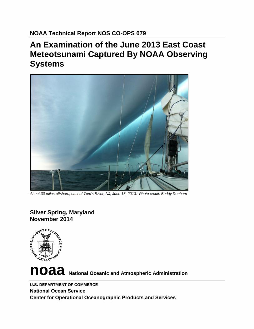
About 30 miles offshore, east of Tom’s River, NJ, June 13, 2013. Photo credit: Buddy Denham

Silver Spring, Maryland November 2014

noaa National Oceanic and Atmospheric Administration

U.S. DEPARTMENT OF COMMERCE National Ocean Service Center for Operational Oceanographic Products and Services

Center for Operational Oceanographic Products and Services National Ocean Service

National Oceanic and Atmospheric Administration U.S. Department of Commerce

The National Ocean Service (NOS) Center for Operational Oceanographic Products and Services (CO-OPS) provides the National infrastructure, science, and technical expertise to collect and distribute observations and predictions of water levels and currents to ensure safe, efficient and environmentally sound maritime commerce. The Center provides the set of water level and tidal current products required to support NOS’ Strategic Plan mission requirements, and to assist in providing operational oceanographic data/products required by NOAA’s other Strategic Plan themes. For example, CO-OPS provides data and products required by the National Weather Service to meet its flood and tsunami warning responsibilities. The Center manages the National Water Level Observation Network (NWLON), a national network of Physical Oceanographic Real-Time Systems (PORTS®) in major U. S. harbors, and the National Current Observation Program consisting of current surveys in near shore and coastal areas utilizing bottom mounted platforms, subsurface buoys, horizontal sensors and quick response real time buoys. The Center establishes standards for the collection and processing of water level and current data; collects and documents user requirements which serve as the foundation for all resulting program activities; designs new and/or improved oceanographic observing systems; designs software to improve CO-OPS’ data processing capabilities; maintains and operates oceanographic observing systems; performs operational data analysis/quality control; and produces/disseminates oceanographic products.

NOAA Technical Report NOS CO-OPS 079

An Examination of the June 2013 East Coast Meteotsunami Captured by NOAA Observing Systems

Kathleen Bailey Christopher DiVeglio Ashley Welty

November 2014

U.S.DEPARTMENT OF COMMERCE Penny Pritzker, Secretary

National Oceanic and Atmospheric Administration Dr. Kathryn Sullivan, NOAA Administrator and Under Secretary of Commerce for Oceans and Atmosphere

National Ocean Service Dr. Holly Bamford, Assistant Administrator

Center for Operational Oceanographic Products and Services Richard Edwing, Director

NOTICE

Mention of a commercial company or product does not constitute an endorsement by NOAA. Use of information from this publication for publicity or advertising purposes concerning proprietary products or the tests of such products is not authorized.

ii

TABLE OF CONTENTS

List of Figures ............................................................................................................................... iv

List of Tables ................................................................................................................................ vi

Executive Summary .................................................................................................................... vii

Introduction ................................................................................................................................... 1

Meteotsunami Characteristics ..................................................................................................... 3

Atmospheric Disturbance ............................................................................................................ 3

External Resonance ..................................................................................................................... 3

Internal Resonance ...................................................................................................................... 4

Meteotsunami Events.................................................................................................................... 7

Global Occurrences .................................................................................................................... 8

U.S. Occurrences....................................................................................................................... 10

The June 2013 Meteotsunami .................................................................................................... 13

Meteotsunami Formation and Impact ....................................................................................... 16

Approaching the shelf break .................................................................................................. 17

Past the shelf break................................................................................................................ 19

U.S. East Coast Impact ............................................................................................................. 22

New Jersey Coast................................................................................................................... 25

Narragansett Bay ................................................................................................................... 26

Woods Hole/Falmouth Harbor .............................................................................................. 26

Long Island Sound ................................................................................................................. 28

Current Meter data ................................................................................................................ 29

Discussion..................................................................................................................................... 35

The Atlantic Basin and wave dynamics ..................................................................................... 35

Conclusion ................................................................................................................................... 37

Acknowledgements ..................................................................................................................... 39

References .................................................................................................................................... 40

iii

LIST OF FIGURES

Figure 1. The generation and evolution of a meteotsunami, adapted from Monserrat 2006. A wave is generated by an atmospheric pressure jump, and becomes amplified by Proudman resonance and harbor resonance as it propagates towards the shore. ........... 4

Figure 2. Source events that generated a tsunami. Validity of the tsunami ranges from very doubtful to definite. The red bar indicates derived information that is estimated from source data. Source: The National Geophysical Data Center Tsunami Database (June, 2014). .............................................................................................................................. 7

Figure 3.Global locations where documented meteotsunamis have occurred: Nagasaki Bay, Japan (a); Ciutadella Harbor, Menorca Island, Spain (b); and the Adriatic Sea (c). ...... 9

Figure 4. Northeast CONUS surface analysis on June 13, 2013 12:00 UTC showing the low pressure system. Source: NOAA/NWS/WPC ............................................................. 13

Figure 5. 8537121 Ship John Shoal, NJ barometric pressure time series indicating a 3.0-mb jump over six minutes from 14:12 to 14:18 UTC (red arrow). .................................... 15

Figure 6. Sea depth contour map (in meters). Red lines indicate the storm position at three different times. Source: NOAA/NESDIS/NGDC. Radar imagery at 15:00 UTC (left), 16:00 UTC (middle) and 17:00 UTC (right). Source: NOAA/National Climatic Data Center. .......................................................................................................................... 16

Figure 7. From Knight et al. (2013). A simulation from the adjusted 2-D Alaska Tsunami Forecast Model. The wave reflected off the shelf break 120 minutes after the pressure perturbation crossed the coast (left) and at 180 minutes the reflected wave propagated northwest towards the coast (right). ............................................................................. 18

Figure 8. From Wang et al. (2013). A simulation from the adjusted RIFT model depicting the wave travel time and impact at 18:05 UTC as it moved northwest towards the U.S. coast (upper) and 23:28 UTC as it reverberated throughout the shelf (lower). ............ 18

Figure 9. Water column height measured by the DART® buoy 44402 on June 13, 2013. An increase in height indicates the initial meteotsunami passage around 17:00 UTC, and a reflected wave passed around 20:20 UTC. ................................................................... 19

Figure 10. RIFT simulations at 16:55 UTC (a) and 20:21 UTC (b). The first wave detected by Station 44402 at 16:55 UTC was positive (yellow) and at 20:21 UTC the wave was negative (purple). Source: Wang et al. 2013. ............................................................. 20

Figure 11. One-minute detided water level data measured at 2695540 Bermuda Esso Pier. At 18:25 UTC the station began to measure the meteotsunami oscillations, marked by the red arrow. ...................................................................................................................... 21

Figure 12. One-minute detided water level data measured at 9759938 Mona Island, PR. Approximate arrival time is 20:20 UTC, marked by the red arrow. ............................ 21

Figure 13. A regional comparison of onset times (UTC) and maximum wave height (meters) observed in the detided water level data. Eyewitnesses reported water beginning to recede at 19:30 UTC at Barnegat Inlet, NJ and at 20:00 UTC at Falmouth Harbor, MA. ...................................................................................................................................... 23

iv

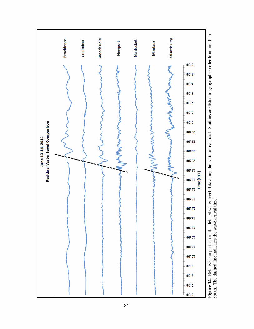
Figure 14. Relative comparison of the detided water level data along the eastern seaboard. Stations are listed in geographic order from north to south. The dashed line indicates the wave arrival time. ................................................................................................... 24

Figure 15. NOAA one-minute detided water level data and six-minute air pressure data measured at 8534720 Atlantic City, NJ. The 3-hour lag (15:00 – 18:05 UTC) between events is indicated by the arrow. .................................................................................. 25

Figure 16. One-minute detided water level data measured at 8452660 Newport, RI. The onset time was at 19:02 UTC. ................................................................................................ 26

Figure 17. One-minute detided water level data measured at 8447930 Woods Hole, MA. The onset time was at 19:28 UTC. ...................................................................................... 27

Figure 18. 8447930 Woods Hole, MA water level station identified by the blue marker (left) and Falmouth Harbor, MA (right). The enclosed, narrow shape of Falmouth Harbor is conducive to wave amplification. ................................................................................. 27

Figure 19. 8449130 Nantucket Island, MA, identified by the blue marker, located in Nantucket Harbor on the north side of the island. ......................................................................... 28

Figure 20. Locations of NOAA water level stations around the Long Island Sound. ................. 29 Figure 21. Location of the 8461490 New London water level station and the nl0101Groton, Pier

6, current meter, located in the Thames River, CT. These stations are 3 km apart. ..... 30 Figure 22. The nl0101 Groton, Pier 6 pressure sensor depth (red curve) and the 8461490 New

London water levels (blue curve). The dashed line at 16:00 UTC denotes the onset of the oscillations. Data are detided, and adjusted for relative comparison. ................... 30

Figure 23. Radar imagery from the second round of storms over the Chesapeake Bay at 20:30 UTC. The storm is oriented northeast-southwest. A subset of NOAA stations is shown. Source: NOAA/National Climatic Data Center. ............................................. 31

Figure 24. Comparison of detided one-minute water level data at Chesapeake Bay stations. Red dashed lines indicate the storm arrival. ........................................................................ 33

Figure 25. Lower Chesapeake Bay detided water level data. Yorktown, VA (blue) is on the west side of the Bay, and Kiptopeke, VA (red) is on the east side. ...................................... 34

v

LIST OF TABLES

Table 1. Maximum observed wind speeds and gusts and air pressure jumps during the storm. Gray boxes indicate locations where maximum gusts did not exceed 20 kt or wind data were not available. ........................................................................................................ 15

Table 2. Water level characteristics observed at NOAA water level stations affected by the meteotsunami. Stations are ordered by maximum wave height. .................................. 22

Table 3. Maximum observed wind speeds and gusts during the second round of the June 13 storms. Stations shown are located in the Chesapeake Bay and ordered from north to south. ............................................................................................................................ 31

vi

EXECUTIVE SUMMARY

On June 13, 2013, a weakening low-end derecho exited eastward off the New Jersey coastline around 15:00 UTC. Three to five hours later, tsunami-like waves were observed in Barnegat Inlet, NJ and Falmouth Harbor, MA despite clear skies and calm weather. The United States Geological Survey as well as the National Tsunami Warning Center suggested that these waves were generated by a meteorological source.

Meteotsunamis are tsunami-like waves of meteorological origin, rather than of seismic origin. The storm had triggered an ocean wave that traveled eastward and reflected off the continental shelf break, causing waves to propagate back to the U.S. East Coast. A huge area was affected, and several NOAA water level stations located along the New Jersey and New England coasts as well as in Bermuda and Puerto Rico captured the meteotsunami oscillations. This report describes the storm that caused the meteotsunami and examines the wave characteristics using high-frequency detided water level data from the NOAA stations. These stations are located in bays and inlets as well as the open coast, and show how the impact varied along the U.S. coastline. Observations from a NOAA buoy located east of the shelf break are also examined along with output from adjusted Tsunami Warning Center models (from other NOAA studies) to illustrate the complexity and timing of the event.

Recent research funded by a NOAA grant for developing a meteotsunami warning program revealed that East Coast meteotsunamis are relatively common, and that the coast is at a higher risk of a meteotsunami than a tsunami. Numerous case studies are being used to develop potential methods for meteotsunami forecasting, although quantitative forecasts/warnings are a challenge based on the complexity of these events. Regardless, as a result of the NOAA grant local weather forecast offices have been able to identify atmospheric conditions conducive to meteotsunami formation and have included warnings for potential surges in area forecasts.

vii

INTRODUCTION

On June 13, 2013 around 19:30 UTC, an eyewitness in Barnegat Inlet, NJ was spearfishing just south of the northern submerged breakwater when he suddenly noticed a strong outflow of water that lasted a couple of minutes, pulling divers seaward over the breakwater. The breakwater, which is normally submerged by about 0.9 to 1.2 m (3 to 4 ft), became exposed. Then he saw an approximately 2-m (6-ft) peak-to-trough wave approaching, carrying the divers back into the inlet. It smashed into the south jetty, knocking three people into the water. The weather by contrast was calm - overcast with a light wind out of the east. At about 20:00 UTC that same day, residents in Falmouth Harbor, MA witnessed a sudden retreat of water out of the harbor, followed by a sudden influx minutes later. The waters continued to surge in and out of the harbor for the next hour, puzzling bystanders. These events were eerily characteristic of a tsunami, but there were no reports or warnings indicating that an offshore earthquake capable of generating a tsunami was expected. USGS Woods Hole was the first group to publicly suggest that a meteotsunami (a tsunami of meteorological origin) had hit the East Coast. Shortly thereafter, the NOAA National Tsunami Warning Center (NTWC) announced that the event was a meteotsunami to the Tsunami Bulletin Board.

Identifying a meteotsunami is a challenge because its characteristics are almost indistinguishable from a seismic tsunami. Even if a large seismic event is not detected, an underwater landslide could still trigger a tsunami. Furthermore, a meteotsunami can be confused with wind-driven storm surge and normal seiche activity. These various uncertainties have made it difficult to predict and thus warn the general public of an event. In certain parts of the world, however, meteotsunamis are relatively common and numerous case studies have elucidated the dynamics of these events. In general, these events occurred from a traveling atmospheric disturbance generating a wave that propagated towards the shore, specifically an inlet with certain resonance properties that amplified the wave. For most U.S. East Coast meteotsunamis, however, typical meteotsunami impacts are more counterintuitive because storm systems moving offshore generate an onshore wave.

In 2011, NOAA awarded a grant (Funding Opportunity Number NOAA-NWS-NWSPO-2011-2002833) to an international group of scientists to examine U.S. East Coast meteotsunamis that occurred from 2010 to 2012. The project was motivated by a 2008 meteotsunami in Boothbay, ME that uncovered a need for a warning system. The project goals were to identify initial conditions conducive to meteotsunami generation, identify observing and processing systems necessary for meteotsunami forecasting, and develop warning protocols for the U.S. The results of this grant have enabled NOAA to identify forecasted storms as possible meteotsunami sources and provide warnings to the public for the possibility of coastal surges.

This report discusses the June 2013 meteotsunami recorded by several NOAA water level stations. Meteotsunami characteristics are defined and examples of global and U.S. events are provided. The meteorological conditions that caused the event are described and the water level response is examined across the Atlantic Ocean as well as along the U.S. East Coast. The influence of bathymetry and its effect on the wave dynamics is discussed with reference to published literature. This report concludes with a summary of efforts leading towards an

1

established quantitative forecast/warning system that would give people ample time to clear the area in the event of a meteotsunami.

2

METEOTSUNAMI CHARACTERISTICS

A tsunami is a series of ocean waves that are typically generated by an underwater geological event such as an earthquake, volcanic eruption, or a submarine landslide. The resulting abrupt change in sea-surface height sends a set of long waves propagating outward from the point of origin. As the waves approach the coastline and the water shoals, they are amplified and can be extremely destructive, depending on the shape of the coastline and the bathymetry. A meteotsunami is very similar to a tsunami in that they are shallow-water gravity waves that are affected by ocean depth, and propagate and evolve in the same manner; however, the origin of these waves differs.

Atmospheric Disturbance

Meteotsunamis are generated by traveling atmospheric disturbances, such as frontal passages, gravity waves, squall lines, and significant pressure jumps. Gravity waves form when air parcels are lifted due to buoyancy and then pulled down by gravity in an oscillating manner. This can occur when air passes over mountain chains. The pressure perturbations associated with these disturbances have been identified as sources of atmospheric forcing that translate energy to the ocean surface (Hibiya and Kajiura 1982; Monserrat 1991; Mercer 2002). A pressure change causes a minor change in sea level due to the inverted barometer effect. For example, a pressure jump of 3 mb causes the sea level to drop by about 3 cm. Figure 1 illustrates the generation and evolution of a meteotsunami, beginning with this pressure jump. However, it is important to note that a passing disturbance will not necessarily trigger a meteotsunami unless resonance occurs.

External Resonance

Resonance occurs when the speed of the pressure perturbation matches the speed of the ocean wave. At this point, the atmospherically-forced energy transfer can generate and energize long ocean surface waves, inducing a significant sea level response (Renault 2011, Vilibić et al. 2008, Monserrat et al. 2006). Different types of resonance can take place depending on the region, but the most relevant types include Proudman resonance (Proudman 1929), Greenspan resonance (Greenspan 1956) and shelf resonance. Proudman resonance is the most important type for meteotsunami generation on the U.S. East Coast and is produced when the speed of the atmospheric disturbance, U, matches the phase speed of the ocean wave, c:

𝑈𝑈 = 𝑐𝑐 = �𝑔𝑔𝑔𝑔,

where g is gravity and H is the depth of the water column beneath the traveling pressure perturbation. This resonance is also demonstrated in Figure 1, where the wave becomes amplified as it travels towards the shore. Greenspan resonance applies to traveling atmospheric disturbances and associated waves moving alongshore. It is important for meteotsunami generation in the Great Lakes, especially because of strong wind forcing in shallow areas (Bechle and Wu 2014). In all cases, the conditions exist where the surface gravity wave becomes amplified. This external resonance alone will not necessarily result in a destructive meteotsunami on the East Coast. As the waves propagate towards shore, the potential for coastal inundation will be maximized in semi-enclosed water bodies where internal resonance occurs.

3

4

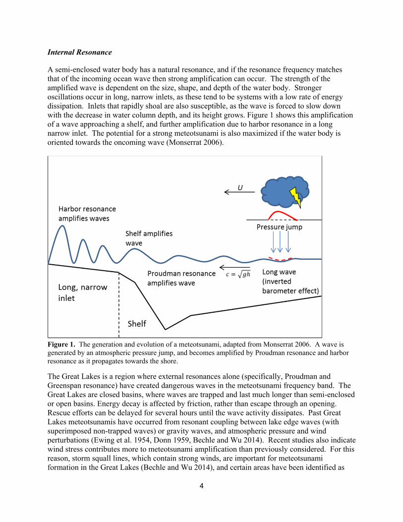
Internal Resonance A semi-enclosed water body has a natural resonance, and if the resonance frequency matches that of the incoming ocean wave then strong amplification can occur. The strength of the amplified wave is dependent on the size, shape, and depth of the water body. Stronger oscillations occur in long, narrow inlets, as these tend to be systems with a low rate of energy dissipation. Inlets that rapidly shoal are also susceptible, as the wave is forced to slow down with the decrease in water column depth, and its height grows. Figure 1 shows this amplification of a wave approaching a shelf, and further amplification due to harbor resonance in a long narrow inlet. The potential for a strong meteotsunami is also maximized if the water body is oriented towards the oncoming wave (Monserrat 2006).

Figure 1. The generation and evolution of a meteotsunami, adapted from Monserrat 2006. A wave is generated by an atmospheric pressure jump, and becomes amplified by Proudman resonance and harbor resonance as it propagates towards the shore.

The Great Lakes is a region where external resonances alone (specifically, Proudman and Greenspan resonance) have created dangerous waves in the meteotsunami frequency band. The Great Lakes are closed basins, where waves are trapped and last much longer than semi-enclosed or open basins. Energy decay is affected by friction, rather than escape through an opening. Rescue efforts can be delayed for several hours until the wave activity dissipates. Past Great Lakes meteotsunamis have occurred from resonant coupling between lake edge waves (with superimposed non-trapped waves) or gravity waves, and atmospheric pressure and wind perturbations (Ewing et al. 1954, Donn 1959, Bechle and Wu 2014). Recent studies also indicate wind stress contributes more to meteotsunami amplification than previously considered. For this reason, storm squall lines, which contain strong winds, are important for meteotsunami formation in the Great Lakes (Bechle and Wu 2014), and certain areas have been identified as

potential ‘hotspots’ (depending on the strength and movement of the storm) where oscillations become amplified (Šepić and Rabinovich 2014). Lake Michigan and eastern Lake Erie have been identified as hotspots to observe during future events.

5

METEOTSUNAMI EVENTS

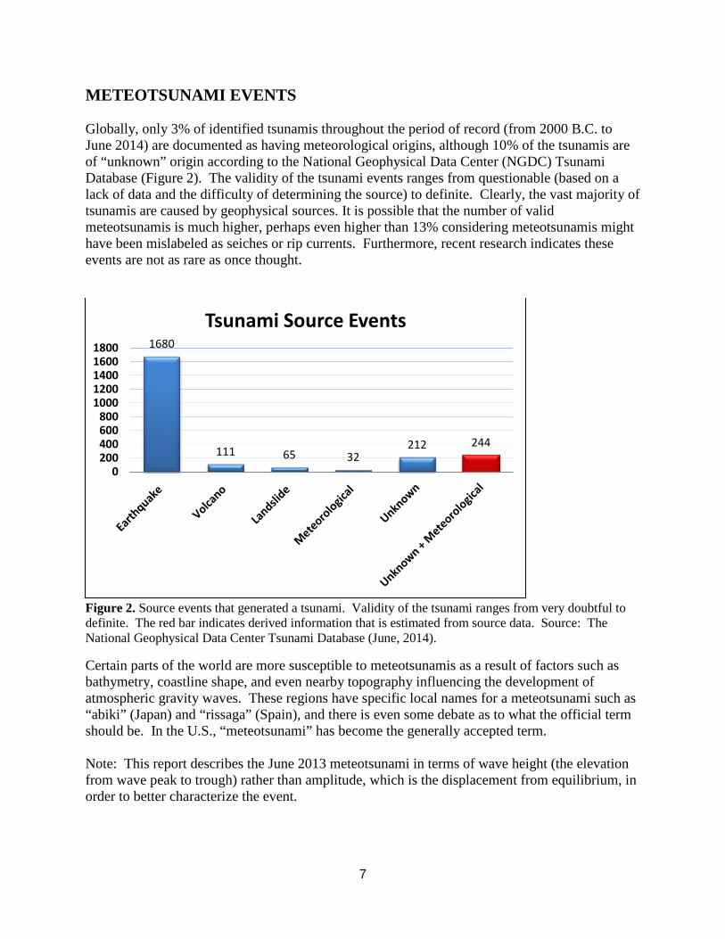
Globally, only 3% of identified tsunamis throughout the period of record (from 2000 B.C. to June 2014) are documented as having meteorological origins, although 10% of the tsunamis are of “unknown” origin according to the National Geophysical Data Center (NGDC) Tsunami Database (Figure 2). The validity of the tsunami events ranges from questionable (based on a lack of data and the difficulty of determining the source) to definite. Clearly, the vast majority of tsunamis are caused by geophysical sources. It is possible that the number of valid meteotsunamis is much higher, perhaps even higher than 13% considering meteotsunamis might have been mislabeled as seiches or rip currents. Furthermore, recent research indicates these events are not as rare as once thought.

Figure 2. Source events that generated a tsunami. Validity of the tsunami ranges from very doubtful to definite. The red bar indicates derived information that is estimated from source data. Source: The National Geophysical Data Center Tsunami Database (June, 2014).

Certain parts of the world are more susceptible to meteotsunamis as a result of factors such as bathymetry, coastline shape, and even nearby topography influencing the development of atmospheric gravity waves. These regions have specific local names for a meteotsunami such as “abiki” (Japan) and “rissaga” (Spain), and there is even some debate as to what the official term should be. In the U.S., “meteotsunami” has become the generally accepted term.

Note: This report describes the June 2013 meteotsunami in terms of wave height (the elevation from wave peak to trough) rather than amplitude, which is the displacement from equilibrium, in order to better characterize the event.

1680

111 65 32 212 244

0200400600800

10001200140016001800

Tsunami Source Events

7

Global Occurrences

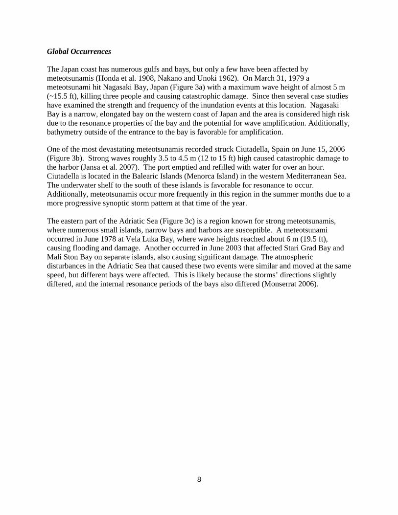
The Japan coast has numerous gulfs and bays, but only a few have been affected by meteotsunamis (Honda et al. 1908, Nakano and Unoki 1962). On March 31, 1979 a meteotsunami hit Nagasaki Bay, Japan (Figure 3a) with a maximum wave height of almost 5 m (~15.5 ft), killing three people and causing catastrophic damage. Since then several case studies have examined the strength and frequency of the inundation events at this location. Nagasaki Bay is a narrow, elongated bay on the western coast of Japan and the area is considered high risk due to the resonance properties of the bay and the potential for wave amplification. Additionally, bathymetry outside of the entrance to the bay is favorable for amplification.

One of the most devastating meteotsunamis recorded struck Ciutadella, Spain on June 15, 2006 (Figure 3b). Strong waves roughly 3.5 to 4.5 m (12 to 15 ft) high caused catastrophic damage to the harbor (Jansa et al. 2007). The port emptied and refilled with water for over an hour. Ciutadella is located in the Balearic Islands (Menorca Island) in the western Mediterranean Sea. The underwater shelf to the south of these islands is favorable for resonance to occur. Additionally, meteotsunamis occur more frequently in this region in the summer months due to a more progressive synoptic storm pattern at that time of the year.

The eastern part of the Adriatic Sea (Figure 3c) is a region known for strong meteotsunamis, where numerous small islands, narrow bays and harbors are susceptible. A meteotsunami occurred in June 1978 at Vela Luka Bay, where wave heights reached about 6 m (19.5 ft), causing flooding and damage. Another occurred in June 2003 that affected Stari Grad Bay and Mali Ston Bay on separate islands, also causing significant damage. The atmospheric disturbances in the Adriatic Sea that caused these two events were similar and moved at the same speed, but different bays were affected. This is likely because the storms’ directions slightly differed, and the internal resonance periods of the bays also differed (Monserrat 2006).

8

a.

b.

c. Figure 3. Global locations where documented meteotsunamis have occurred: Nagasaki Bay, Japan (a); Ciutadella Harbor, Menorca Island, Spain (b); and the Adriatic Sea (c).

9

U.S. Occurrences

Several meteotsunamis have occurred in the Great Lakes. The most notable one occurred on June 26, 1954 in Lake Michigan. A massive wave about 3 m (10 ft) high swept several people off piers near Chicago, IL, killing seven. Storms had passed through the region two hours earlier, but the weather was hot and sunny when the wave struck. At the time, the Weather Bureau noted that these types of sudden surge events were always associated with a passing squall line and a pressure jump. Following the June 26 event, forecasters were instructed to look for storms with a particular speed and direction that might generate these large waves. When another large meteotsunami struck only ten days later on July 6 with a wave height of about 1.25 m (~4 ft), warnings were issued in time and there were no fatalities (Hughes 1965). Bechle and Wu (2014) revisited these events and concluded from numerical hydrodynamic model simulations that the amplitudes of the 1954 waves were dependent on both pressure and wind perturbations, and that the storms also produced edge waves that lasted several hours in the enclosed basin. The June 26 wave that hit Chicago was a reflected wave propagating westward from the southeast coast of Lake Michigan, whereas the July 6 event was a result of superimposed edge waves.

Another well-documented meteotsunami occurred at Daytona Beach, FL on July 3-4, 1992 around midnight local time (Sallenger et al. 1995, Churchill et al. 1995). A wave 3 m (10 ft) high crashed onto shore, causing damage to several vehicles and injuring dozens of people. A southward moving squall line situated just north of the area resonantly generated long ocean waves that propagated towards the shore. This squall line did not affect local meteorological conditions, so there was no indication that an onshore wave of this magnitude was approaching. The effects could have been much worse if the wave hit hours later during daylight hours while July 4th festivities were occurring.

On October 28, 2008, large waves hit Boothbay, ME. Similar to the 2013 event witnessed at Falmouth Harbor, water suddenly rushed into Boothbay Harbor, rose up to 3.5 m (12 ft) for 15 minutes, and then suddenly receded. This pattern repeated itself at least three times, causing damage to the shoreline infrastructure. Vilibić et al. (2014) determined that an earlier cold front that moved through the area contained internal gravity waves that generated a meteotsunami along the Gulf of Maine shelf. Whitmore and Knight (2014) also correlated wave heights in Boothbay with the atmospheric jump using a tsunami forecast model. In general, this event was heavily examined and was used as a test case to begin developing forecasting capabilities on the U.S. East Coast.

On June 29-30, 2012 a large and destructive derecho rapidly traveled across the Great Lakes to the Mid-Atlantic region. A derecho is a widespread and usually fast-moving windstorm associated with or embedded in convection and can produce damaging straight-line winds over areas hundreds of miles long and more than 100 miles across. NOAA observing systems measured a substantial pressure jump (7.3 mb over 30 minutes at Chesapeake City, MD) and maximum wind gusts of up to 75 kt. There was no meteotsunami-induced damage, and wave heights only ranged from 0.15 m (0.5 ft) along the Atlantic Coast to 0.5 m (1.65 ft) in the upper Chesapeake Bay. The upper Chesapeake Bay oscillations were a direct response to wind stress, which is typical for high-wind events in this area. Water level oscillations along the Atlantic

10

coast (from Duck, NC to Sandy Hook, NJ) were observed one to three hours after the storms passed, which is a similar to the delayed response seen during the June 2013 meteotsunami (Šepić and Rabinovich 2014).

11

THE JUNE 2013 METEOTSUNAMI NOAA initially examined the June 2013 event to determine if the source was seismic. A review of seismograph data did not reveal any evidence of an earthquake that might trigger a tsunami. An underwater landslide was ruled out after the NOAA research vessel Okeanos Explorer examined the Hudson River Canyon and determined that there was no sediment displacement. Post-event analyses (Knight et al. 2013, Wang et al. 2013) confirmed that an earlier weather system moving offshore was the source of the tsunami, and the USGS has recorded the event as a validated meteotsunami.

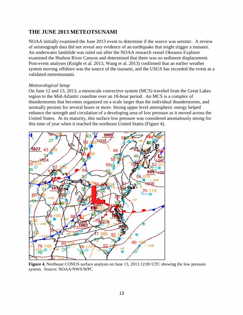
Meteorological Setup On June 12 and 13, 2013, a mesoscale convective system (MCS) traveled from the Great Lakes region to the Mid-Atlantic coastline over an 18-hour period. An MCS is a complex of thunderstorms that becomes organized on a scale larger than the individual thunderstorms, and normally persists for several hours or more. Strong upper level atmospheric energy helped enhance the strength and circulation of a developing area of low pressure as it moved across the United States. At its maturity, this surface low pressure was considered anomalously strong for this time of year when it reached the northeast United States (Figure 4).

Figure 4. Northeast CONUS surface analysis on June 13, 2013 12:00 UTC showing the low pressure system. Source: NOAA/NWS/WPC

13

On June 12th, the MCS became well-developed over northern Indiana, with an average forward speed of 21 m/s (41 kt) moving in an east-southeast direction. Preliminary NWS reports indicated that this MCS produced a derecho on the lower end of the spectrum mainly because of its smaller size. The MCS and the associated low-end derecho caused widespread damage, mostly from straight line winds across Indiana, Ohio and Pennsylvania.

Between 11:30 UTC and 15:00 UTC on June 13th, the MCS extended from just south of New York City to the Washington, D.C. metropolitan area. A severe thunderstorm watch was issued for southeast Pennsylvania, the southern half of New Jersey, Delaware and eastern Maryland. The thunderstorms passed through Philadelphia and crossed the Delaware River between 13:30 UTC and 14:30 UTC before continuing to move rapidly across New Jersey. As the storms approached the coastline they failed to reach severe criteria (winds of 50 kt and/or hail at least 1 inch in diameter) and there wasn’t much damage caused as a result. The storms then cleared the New Jersey coast by 15:30 UTC.

Table 1 provides maximum wind speeds and gusts as well as barometric pressure jumps recorded at several NOAA stations located in the path of the storms. The NOAA/NOS stations are identified by 7-digit IDs and NWS stations are identified by 4-character IDs (airport codes). The pressure jump values in Table 1 indicate the increase over the duration that the increase occurred. Overall, peak wind gusts across eastern Pennsylvania, New Jersey and Delaware ranged from 20 to 40 kt at most observing sites. Millville Airport, NJ and Atlantic City Airport, NJ recorded the highest wind gusts, up to 40 kt and 45 kt, respectively. The associated air pressure jump at Millville Airport, however, was not very intense (1.6 mb change over 30 minutes). The more intense pressure jumps were recorded at Ship John Shoal, NJ (Figure 5), where the pressure rose 3 mb over only 6 minutes, and the Atlantic City airport, where a 4.7-mb jump was recorded over 18 minutes.

Pressure data from the Transportable Array (a network of 400 seismographs spaced every 70 km across the U.S., operated by the Incorporated Research Institutions for Seismology) measured a 6-mb jump as the system moved across Delaware. The extent of the pressure jump, the speed of the system, and the amplitude were gleaned from the several stations to help characterize the system and track the eastward progression of the pressure anomaly (Knight et al. 2013). Historically, meteotsunamis have almost always been associated with pressure jumps (Hibiya and Kajiura 1982, Akamatsu 1978); therefore, this type of pressure disturbance is significant.

14

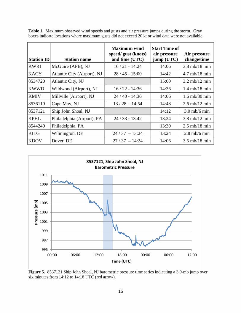
Table 1. Maximum observed wind speeds and gusts and air pressure jumps during the storm. Gray boxes indicate locations where maximum gusts did not exceed 20 kt or wind data were not available.

Station ID Station name

Maximum wind speed/ gust (knots)

and time (UTC)

Start Time of air pressure jump (UTC)

Air pressure change/time

KWRI McGuire (AFB), NJ 16 / 21 - 14:24 14:06 3.8 mb/18 min KACY Atlantic City (Airport), NJ 28 / 45 - 15:00 14:42 4.7 mb/18 min 8534720 Atlantic City, NJ 15:00 3.2 mb/12 min KWWD Wildwood (Airport), NJ 16 / 22 - 14:36 14:36 1.4 mb/18 min KMIV Millville (Airport), NJ 24 / 40 - 14:36 14:06 1.6 mb/30 min 8536110 Cape May, NJ 13 / 28 - 14:54 14:48 2.6 mb/12 min 8537121 Ship John Shoal, NJ 14:12 3.0 mb/6 min KPHL Philadelphia (Airport), PA 24 / 33 - 13:42 13:24 3.8 mb/12 min 8544240 Philadelphia, PA 13:30 2.5 mb/18 min KILG Wilmington, DE 24 / 37 – 13:24 13:24 2.8 mb/6 min KDOV Dover, DE 27 / 37 – 14:24 14:06 3.5 mb/18 min

Figure 5. 8537121 Ship John Shoal, NJ barometric pressure time series indicating a 3.0-mb jump over six minutes from 14:12 to 14:18 UTC (red arrow).

995

997

999

1001

1003

1005

1007

1009

1011

00:00 06:00 12:00 18:00 00:00 06:00 12:00

Pres

sure

(mb)

Time (UTC)

8537121, Ship John Shoal, NJ Barometric Pressure

15

Meteotsunami Formation and Impact

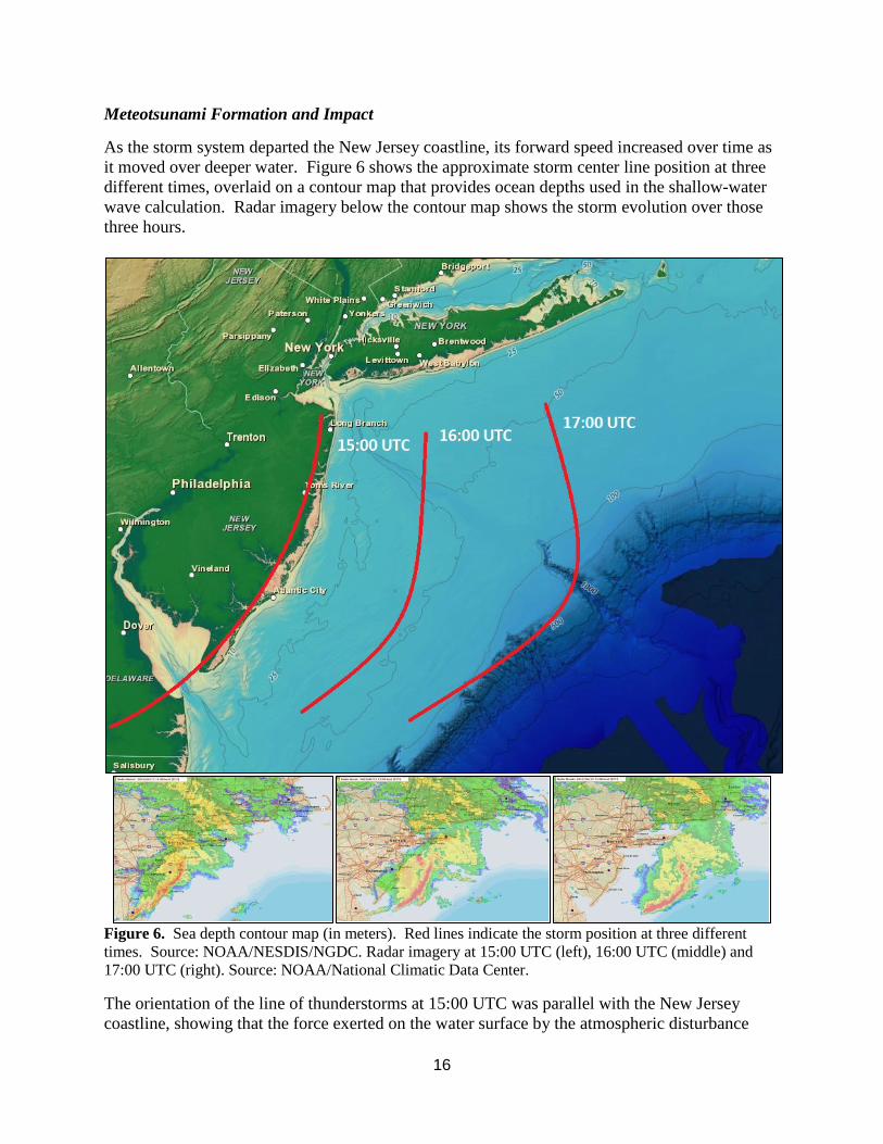
As the storm system departed the New Jersey coastline, its forward speed increased over time as it moved over deeper water. Figure 6 shows the approximate storm center line position at three different times, overlaid on a contour map that provides ocean depths used in the shallow-water wave calculation. Radar imagery below the contour map shows the storm evolution over those three hours.

Figure 6. Sea depth contour map (in meters). Red lines indicate the storm position at three different times. Source: NOAA/NESDIS/NGDC. Radar imagery at 15:00 UTC (left), 16:00 UTC (middle) and 17:00 UTC (right). Source: NOAA/National Climatic Data Center.

The orientation of the line of thunderstorms at 15:00 UTC was parallel with the New Jersey coastline, showing that the force exerted on the water surface by the atmospheric disturbance

16

covered a wide area. By 16:00 UTC the storm system had moved 60 km at a speed of 17 m/s. The average ocean depth was 25 to 50 m within that 60-km distance. This resulted in an ocean wave speed of 16 to 22 m/s, which matches the speed of the storm system. By 17:00 UTC the storm system moved 90 km at a speed of 25 m/s. The average ocean depth was 50 to 100 m, which resulted in an ocean wave of 22 to 31 m/s. The wave speed and storm speed also matched during this time period. Therefore, Proudman resonance was possible after the storm exited the coast.

Approaching the shelf break External resonance and bathymetry are major factors in the direction and magnitude of U.S. East Coast meteotsunamis (Pasquet and Vilibić 2013). The mid-Atlantic shelf break in particular is a critical influence on the meteotsunami. Without the shelf break, the U.S. East Coast would not have been impacted.

Between roughly 17:00 and 17:30 UTC, the storm system and associated ocean wave started to cross the continental shelf break. The shelf break lies approximately 100-120 km off the New Jersey coast. Here, the water depth increases from around 100 m to as much as 1200 m over a distance of only 20 km. The wave speed is directly proportional to depth; therefore a sharp increase in depth would result in a sudden increase in speed. Once the waves encountered the shelf break they reflected back towards the coast. This is one of the unique physical characteristics of a meteotsunami; the generation of a tsunami-like wave from a non-seismic offshore source.

Travel times of the wave from the shelf break to the coast and past the shelf break into the deep ocean are difficult to produce, given that the event was not generated from a point source and also considering the complexity of the wave dynamics in the Atlantic basin. Wang et al. (2013) and Knight et al. (2013) modified NOAA Tsunami Warning Center models to use a pressure jump as the source event, and simulated the observed arrival times and amplitude of the wave. Knight et al. (2013) adjusted the Alaska Tsunami Forecast Model (ATFM) using initial conditions determined from the Transportable Array pressure data, and simulated the wave as it progressed eastward and reflected off the shelf break (Figure 7). Wang et al. (2013) adjusted the Real-time Inundation Forecasting of Tsunamis (RIFT) model to show the wave forced by the pressure anomaly, using a maximum pressure jump of 10 mb (Figure 8). The RIFT simulates wave amplitudes, where a positive amplitude is defined as the wave zero to peak, and a negative amplitude is wave zero to trough. The wave amplitude scale ranges from -1 to 1 m. The RIFT simulation covered 12 hours and showed the energy getting trapped by the shallow shelf, as the waves continually reflected off the shelf break and the U.S. coastline. This reverberation throughout the shelf illustrated the complexity of the event, as shown in Figure 8 (lower) at about 23:30 UTC, after almost 10 hours had elapsed. The simulations as well as results from Pasquet and Vilibić (2013) explain the lag time between the storm passage and the water level rise observed along the East Coast.

17

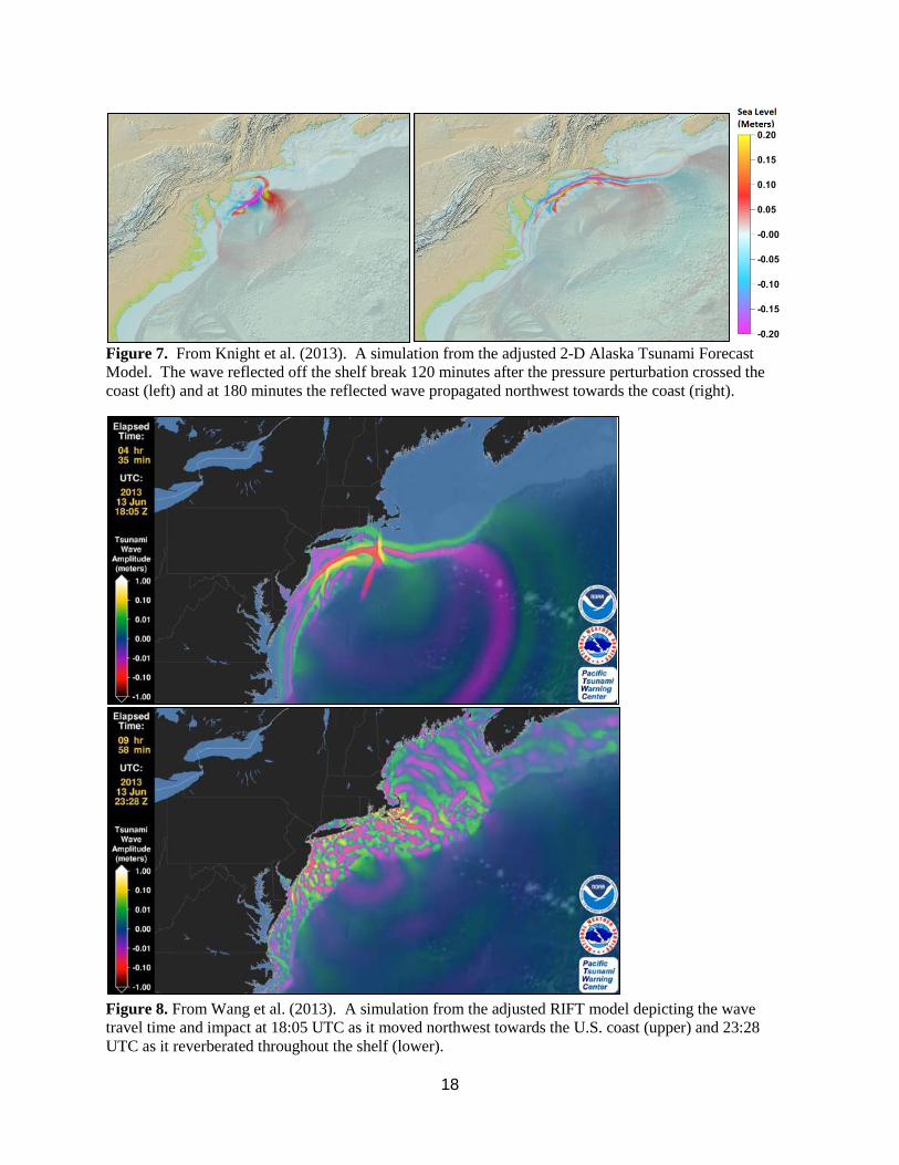
Figure 7. From Knight et al. (2013). A simulation from the adjusted 2-D Alaska Tsunami Forecast Model. The wave reflected off the shelf break 120 minutes after the pressure perturbation crossed the coast (left) and at 180 minutes the reflected wave propagated northwest towards the coast (right).

Figure 8. From Wang et al. (2013). A simulation from the adjusted RIFT model depicting the wave travel time and impact at 18:05 UTC as it moved northwest towards the U.S. coast (upper) and 23:28 UTC as it reverberated throughout the shelf (lower).

18

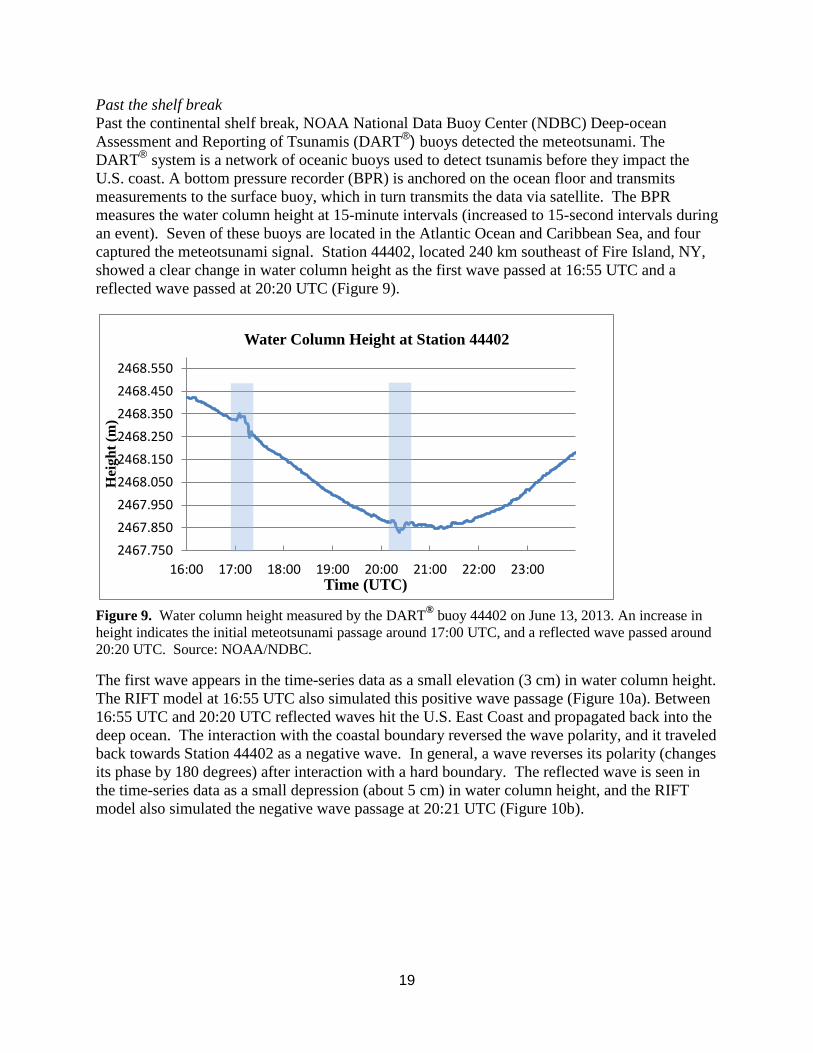
Past the shelf break Past the continental shelf break, NOAA National Data Buoy Center (NDBC) Deep-ocean Assessment and Reporting of Tsunamis (DART®) buoys detected the meteotsunami. The DART® system is a network of oceanic buoys used to detect tsunamis before they impact the U.S. coast. A bottom pressure recorder (BPR) is anchored on the ocean floor and transmits measurements to the surface buoy, which in turn transmits the data via satellite. The BPR measures the water column height at 15-minute intervals (increased to 15-second intervals during an event). Seven of these buoys are located in the Atlantic Ocean and Caribbean Sea, and four captured the meteotsunami signal. Station 44402, located 240 km southeast of Fire Island, NY, showed a clear change in water column height as the first wave passed at 16:55 UTC and a reflected wave passed at 20:20 UTC (Figure 9).

Figure 9. Water column height measured by the DART® buoy 44402 on June 13, 2013. An increase in height indicates the initial meteotsunami passage around 17:00 UTC, and a reflected wave passed around 20:20 UTC. Source: NOAA/NDBC.

The first wave appears in the time-series data as a small elevation (3 cm) in water column height. The RIFT model at 16:55 UTC also simulated this positive wave passage (Figure 10a). Between 16:55 UTC and 20:20 UTC reflected waves hit the U.S. East Coast and propagated back into the deep ocean. The interaction with the coastal boundary reversed the wave polarity, and it traveled back towards Station 44402 as a negative wave. In general, a wave reverses its polarity (changes its phase by 180 degrees) after interaction with a hard boundary. The reflected wave is seen in the time-series data as a small depression (about 5 cm) in water column height, and the RIFT model also simulated the negative wave passage at 20:21 UTC (Figure 10b).

2467.750

2467.850

2467.950

2468.050

2468.150

2468.250

2468.350

2468.450

2468.550

16:00 17:00 18:00 19:00 20:00 21:00 22:00 23:00

Hei

ght (

m)

Time (UTC)

Water Column Height at Station 44402

19

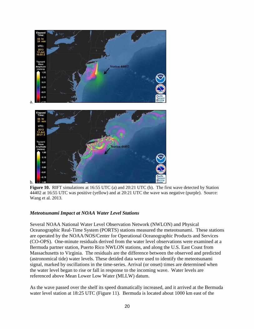
a.

b. Figure 10. RIFT simulations at 16:55 UTC (a) and 20:21 UTC (b). The first wave detected by Station 44402 at 16:55 UTC was positive (yellow) and at 20:21 UTC the wave was negative (purple). Source: Wang et al. 2013.

Meteotsunami Impact at NOAA Water Level Stations

Several NOAA National Water Level Observation Network (NWLON) and Physical Oceanographic Real-Time System (PORTS) stations measured the meteotsunami. These stations are operated by the NOAA/NOS/Center for Operational Oceanographic Products and Services (CO-OPS). One-minute residuals derived from the water level observations were examined at a Bermuda partner station, Puerto Rico NWLON stations, and along the U.S. East Coast from Massachusetts to Virginia. The residuals are the difference between the observed and predicted (astronomical tide) water levels. These detided data were used to identify the meteotsunami signal, marked by oscillations in the time-series. Arrival (or onset) times are determined when the water level began to rise or fall in response to the incoming wave. Water levels are referenced above Mean Lower Low Water (MLLW) datum.

As the wave passed over the shelf its speed dramatically increased, and it arrived at the Bermuda water level station at 18:25 UTC (Figure 11). Bermuda is located about 1000 km east of the

20

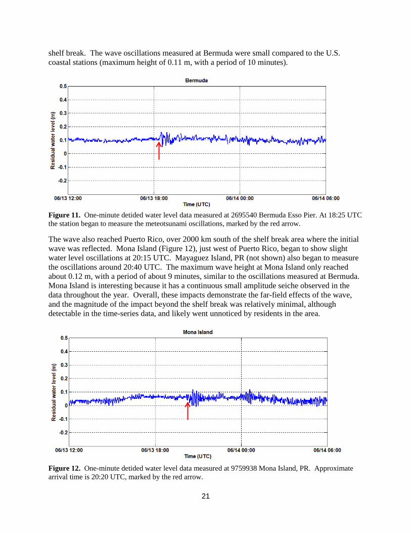
shelf break. The wave oscillations measured at Bermuda were small compared to the U.S. coastal stations (maximum height of 0.11 m, with a period of 10 minutes).

Figure 11. One-minute detided water level data measured at 2695540 Bermuda Esso Pier. At 18:25 UTC the station began to measure the meteotsunami oscillations, marked by the red arrow.

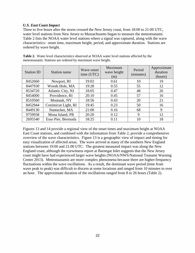
The wave also reached Puerto Rico, over 2000 km south of the shelf break area where the initial wave was reflected. Mona Island (Figure 12), just west of Puerto Rico, began to show slight water level oscillations at 20:15 UTC. Mayaguez Island, PR (not shown) also began to measure the oscillations around 20:40 UTC. The maximum wave height at Mona Island only reached about 0.12 m, with a period of about 9 minutes, similar to the oscillations measured at Bermuda. Mona Island is interesting because it has a continuous small amplitude seiche observed in the data throughout the year. Overall, these impacts demonstrate the far-field effects of the wave, and the magnitude of the impact beyond the shelf break was relatively minimal, although detectable in the time-series data, and likely went unnoticed by residents in the area.

Figure 12. One-minute detided water level data measured at 9759938 Mona Island, PR. Approximate arrival time is 20:20 UTC, marked by the red arrow.

21

U.S. East Coast Impact Three to five hours after the storm crossed the New Jersey coast, from 18:00 to 21:00 UTC, water level stations from New Jersey to Massachusetts began to measure the meteotsunami. Table 2 lists the NOAA water level stations where a signal was captured, along with the wave characteristics: onset time, maximum height, period, and approximate duration. Stations are ordered by wave height.

Table 2. Water level characteristics observed at NOAA water level stations affected by the meteotsunami. Stations are ordered by maximum wave height.

Station ID Station name Wave onset time (UTC)

Maximum wave height

(m)

Period (minutes)

Approximate duration (hours)

8452660 Newport, RI 19:02 0.61 10 19 8447930 Woods Hole, MA 19:28 0.55 55 12 8534720 Atlantic City, NJ 18:05 0.47 48 26 8454000 Providence, RI 20:10 0.45 57 16 8510560 Montauk, NY 18:56 0.43 20 21 8452944 Conimicut Light, RI 19:45 0.23 50 16 8449130 Nantucket, MA 21:00 0.16 68 9 9759938 Mona Island, PR 20:20 0.12 9 12 2695540 Esso Pier, Bermuda 18:25 0.11 10 18

Figures 13 and 14 provide a regional view of the onset times and maximum height at NOAA East Coast stations, and combined with the information from Table 2, provide a comprehensive overview of the wave characteristics. Figure 13 is a geographic view of impact and timing for easy visualization of affected areas. The wave arrived at many of the southern New England stations between 19:00 and 21:00 UTC. The greatest measured impact was along the New England coast, although the eyewitness report at Barnegat Inlet suggests that the New Jersey coast might have had experienced larger wave heights (NOAA/NWS/National Tsunami Warning Center 2013). Meteotsunamis are more complex phenomena because there are higher-frequency fluctuations within the wave oscillations. As a result, the dominant wave period (time from wave peak to peak) was difficult to discern at some locations and ranged from 10 minutes to over an hour. The approximate duration of the oscillations ranged from 8 to 26 hours (Table 2).

22

Figure 13. A regional comparison of onset times (UTC) and maximum wave height (meters) observed in the detided water level data. Eyewitnesses reported water beginning to recede at 19:30 UTC at Barnegat Inlet, NJ and at 20:00 UTC at Falmouth Harbor, MA.

Figure 14 provides a time-series view using one-minute detided water levels measured at the NOAA stations used in Figure 13. The data were adjusted by an arbitrary reference zero for easier comparison. Stations are arranged by latitude (north to south) and the dashed lines indicate how the wave progressed along the coast and up the Narragansett Bay, also seen in Figure 13. The time-series data reveal that some stations measured a clearer, stronger meteotsunami signal than others despite being in the same region. This variability is likely a function of shadowing effects or damping of the wave before it reached the station. In general, the meteotsunami oscillations in the time-series data are detectable, but not as distinct as signals from stronger, seismically-generated tsunamis.

23

Figu

re 1

4. R

elat

ive

com

paris

on o

f the

det

ided

wat

er le

vel d

ata

alon

g th

e ea

ster

n se

aboa

rd.

Stat

ions

are

list

ed in

geo

grap

hic

orde

r fro

m n

orth

to

sout

h. T

he d

ashe

d lin

e in

dica

tes t

he w

ave

arriv

al ti

me.

24

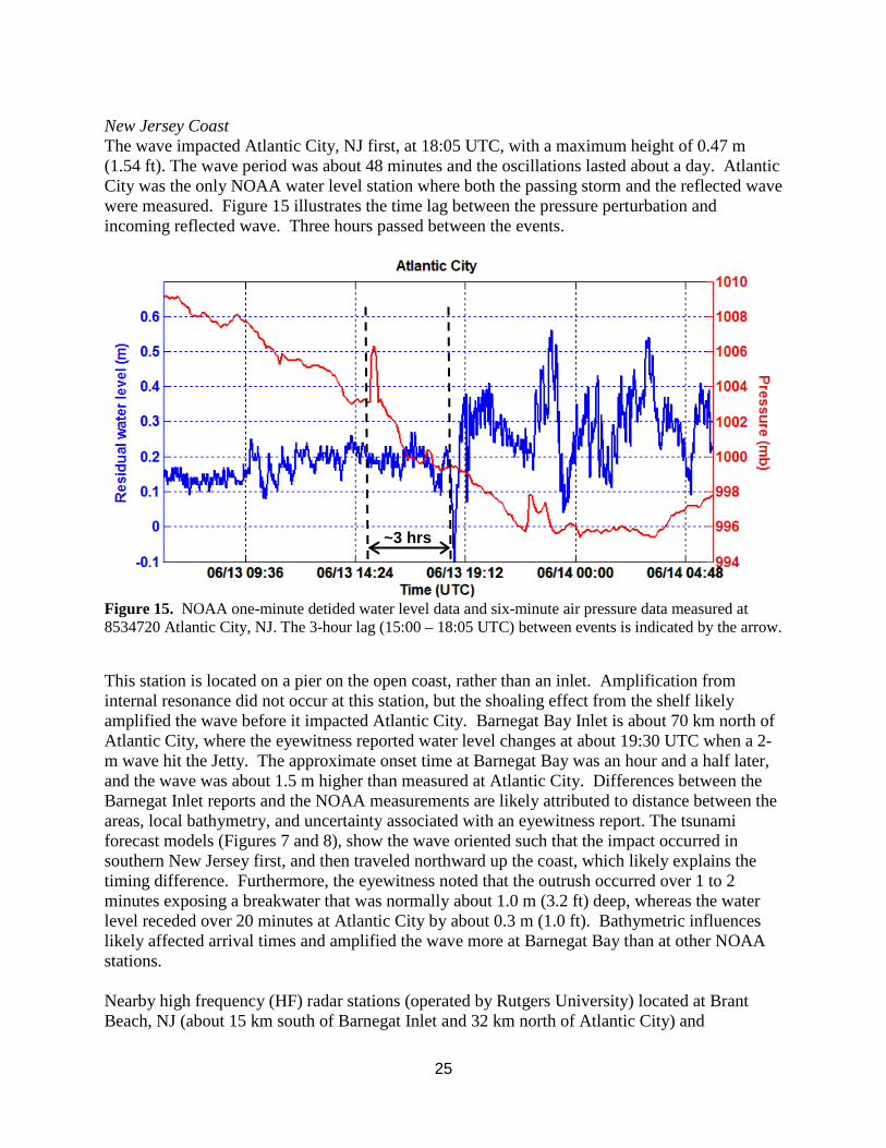
New Jersey Coast The wave impacted Atlantic City, NJ first, at 18:05 UTC, with a maximum height of 0.47 m (1.54 ft). The wave period was about 48 minutes and the oscillations lasted about a day. Atlantic City was the only NOAA water level station where both the passing storm and the reflected wave were measured. Figure 15 illustrates the time lag between the pressure perturbation and incoming reflected wave. Three hours passed between the events.

Figure 15. NOAA one-minute detided water level data and six-minute air pressure data measured at 8534720 Atlantic City, NJ. The 3-hour lag (15:00 – 18:05 UTC) between events is indicated by the arrow.

This station is located on a pier on the open coast, rather than an inlet. Amplification from internal resonance did not occur at this station, but the shoaling effect from the shelf likely amplified the wave before it impacted Atlantic City. Barnegat Bay Inlet is about 70 km north of Atlantic City, where the eyewitness reported water level changes at about 19:30 UTC when a 2-m wave hit the Jetty. The approximate onset time at Barnegat Bay was an hour and a half later, and the wave was about 1.5 m higher than measured at Atlantic City. Differences between the Barnegat Inlet reports and the NOAA measurements are likely attributed to distance between the areas, local bathymetry, and uncertainty associated with an eyewitness report. The tsunami forecast models (Figures 7 and 8), show the wave oriented such that the impact occurred in southern New Jersey first, and then traveled northward up the coast, which likely explains the timing difference. Furthermore, the eyewitness noted that the outrush occurred over 1 to 2 minutes exposing a breakwater that was normally about 1.0 m (3.2 ft) deep, whereas the water level receded over 20 minutes at Atlantic City by about 0.3 m (1.0 ft). Bathymetric influences likely affected arrival times and amplified the wave more at Barnegat Bay than at other NOAA stations.

Nearby high frequency (HF) radar stations (operated by Rutgers University) located at Brant Beach, NJ (about 15 km south of Barnegat Inlet and 32 km north of Atlantic City) and

~3 hrs

25

Brigantine, NJ (about 30 km south of Barnegat Inlet and 8 km north of Atlantic City) detected the incoming wave as well. HF radars measure surface currents, therefore orbital velocities can be derived to detect a tsunami signature. The incoming wave was detected 23 km offshore, almost a full hour before it arrived at the coast. Calculated arrival times from the orbital velocities revealed the wave moved towards the shore at about 8.3 m/s, but arrival times differed along the HF radar array as the wave approached the coastline. In general, the wave reached the coast at the HF radar locations within 30 minutes of the Atlantic City station (Lipa et al. 2013). Different coastal dynamics apparently produced a different response between the measurements at the stations and the actual observations by people on land in both timing and wave height.

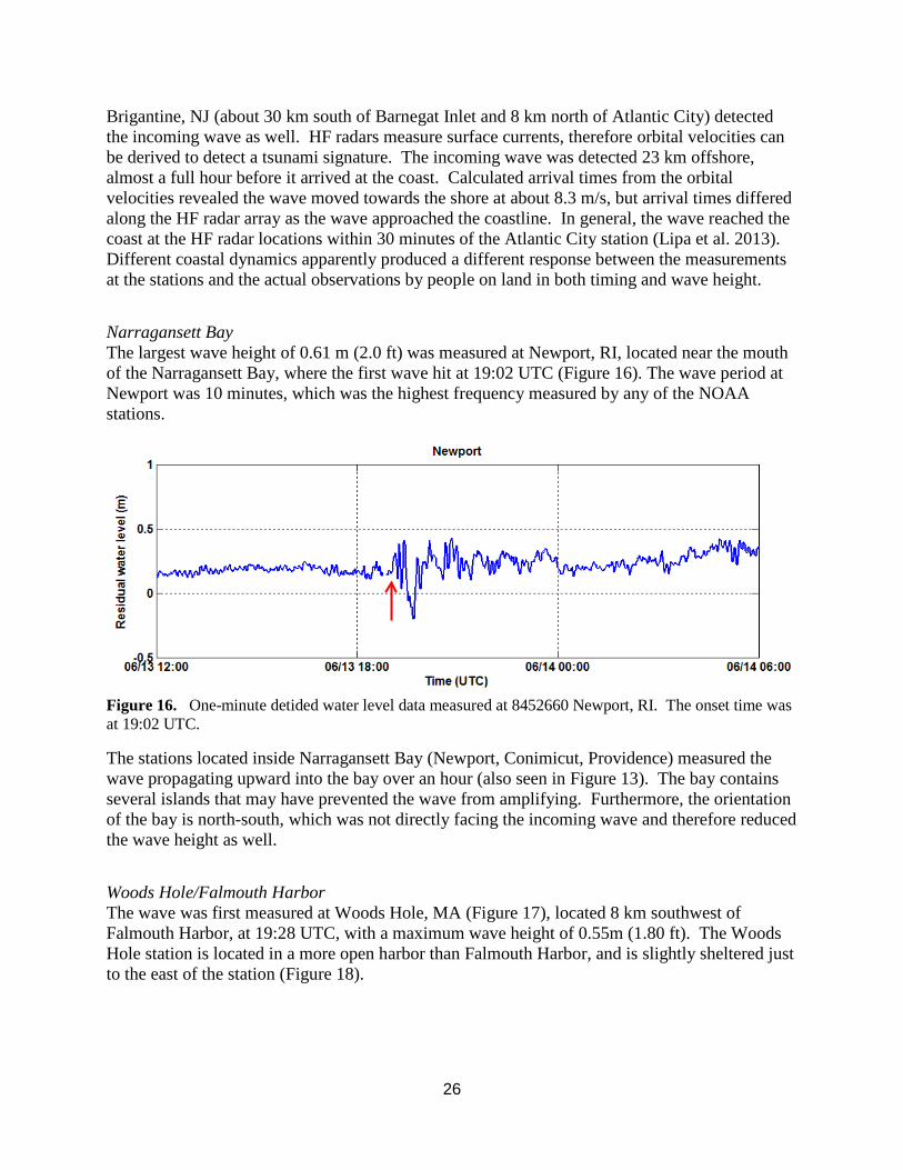
Narragansett Bay The largest wave height of 0.61 m (2.0 ft) was measured at Newport, RI, located near the mouth of the Narragansett Bay, where the first wave hit at 19:02 UTC (Figure 16). The wave period at Newport was 10 minutes, which was the highest frequency measured by any of the NOAA stations.

Figure 16. One-minute detided water level data measured at 8452660 Newport, RI. The onset time was at 19:02 UTC.

The stations located inside Narragansett Bay (Newport, Conimicut, Providence) measured the wave propagating upward into the bay over an hour (also seen in Figure 13). The bay contains several islands that may have prevented the wave from amplifying. Furthermore, the orientation of the bay is north-south, which was not directly facing the incoming wave and therefore reduced the wave height as well.

Woods Hole/Falmouth Harbor The wave was first measured at Woods Hole, MA (Figure 17), located 8 km southwest of Falmouth Harbor, at 19:28 UTC, with a maximum wave height of 0.55m (1.80 ft). The Woods Hole station is located in a more open harbor than Falmouth Harbor, and is slightly sheltered just to the east of the station (Figure 18).

26

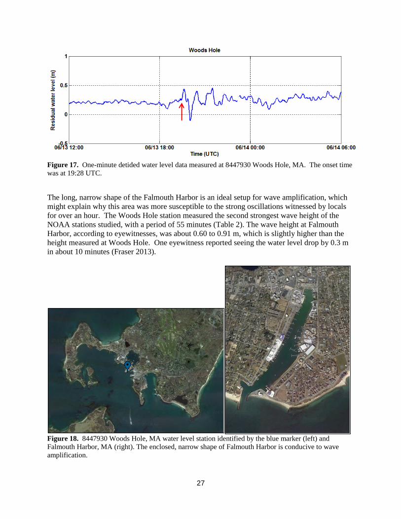
Figure 17. One-minute detided water level data measured at 8447930 Woods Hole, MA. The onset time was at 19:28 UTC.

The long, narrow shape of the Falmouth Harbor is an ideal setup for wave amplification, which might explain why this area was more susceptible to the strong oscillations witnessed by locals for over an hour. The Woods Hole station measured the second strongest wave height of the NOAA stations studied, with a period of 55 minutes (Table 2). The wave height at Falmouth Harbor, according to eyewitnesses, was about 0.60 to 0.91 m, which is slightly higher than the height measured at Woods Hole. One eyewitness reported seeing the water level drop by 0.3 m in about 10 minutes (Fraser 2013).

Figure 18. 8447930 Woods Hole, MA water level station identified by the blue marker (left) and Falmouth Harbor, MA (right). The enclosed, narrow shape of Falmouth Harbor is conducive to wave amplification.

27

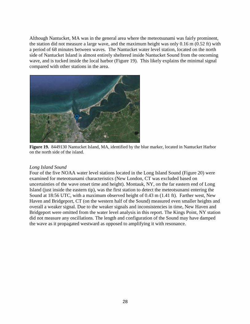
Although Nantucket, MA was in the general area where the meteotsunami was fairly prominent, the station did not measure a large wave, and the maximum height was only 0.16 m (0.52 ft) with a period of 68 minutes between waves. The Nantucket water level station, located on the north side of Nantucket Island is almost entirely sheltered inside Nantucket Sound from the oncoming wave, and is tucked inside the local harbor (Figure 19). This likely explains the minimal signal compared with other stations in the area.

Figure 19. 8449130 Nantucket Island, MA, identified by the blue marker, located in Nantucket Harbor on the north side of the island.

Long Island Sound Four of the five NOAA water level stations located in the Long Island Sound (Figure 20) were examined for meteotsunami characteristics (New London, CT was excluded based on uncertainties of the wave onset time and height). Montauk, NY, on the far eastern end of Long Island (just inside the eastern tip), was the first station to detect the meteotsunami entering the Sound at 18:56 UTC, with a maximum observed height of 0.43 m (1.41 ft). Farther west, New Haven and Bridgeport, CT (on the western half of the Sound) measured even smaller heights and overall a weaker signal. Due to the weaker signals and inconsistencies in time, New Haven and Bridgeport were omitted from the water level analysis in this report. The Kings Point, NY station did not measure any oscillations. The length and configuration of the Sound may have damped the wave as it propagated westward as opposed to amplifying it with resonance.

28

Figure 20. Locations of NOAA water level stations around the Long Island Sound.

Current Meter data Data from several NOAA current meters (measuring underwater current speed and direction) located in the lower Chesapeake, Delaware and Narragansett Bay regions were studied and did not show an abrupt change or abnormal signal in the current speeds and directions due to the meteotsunami. Only one station (Groton, near New London, CT) captured oscillations in its pressure sensor data around the time that the meteotsunami affected the area (around 19:00 UTC). The pressure sensor measures the depth of the sensor underwater. Groton is a side-looking mounted current meter located on the Thames River, approximately 8 km north of the mouth, and 3 km north of the NOAA New London water level station (Figure 21). A comparison of the pressure sensor data and the 6-minute New London water level data shows that oscillations began around 16:00 UTC and lasted for about 9 hours (Figure 22). The onset time of these oscillations was nearly three hours before stations in the area began measuring the meteotsunami. As previously noted, at 16:00 UTC a weather system moved through the area, which could explain the early water level response. It is difficult to tell exactly if and when the meteotsunami affected the Thames River, but the oscillations could be a combination of real-time effects from the weather system and the later influence from the meteotsunami propagating up the river.

29

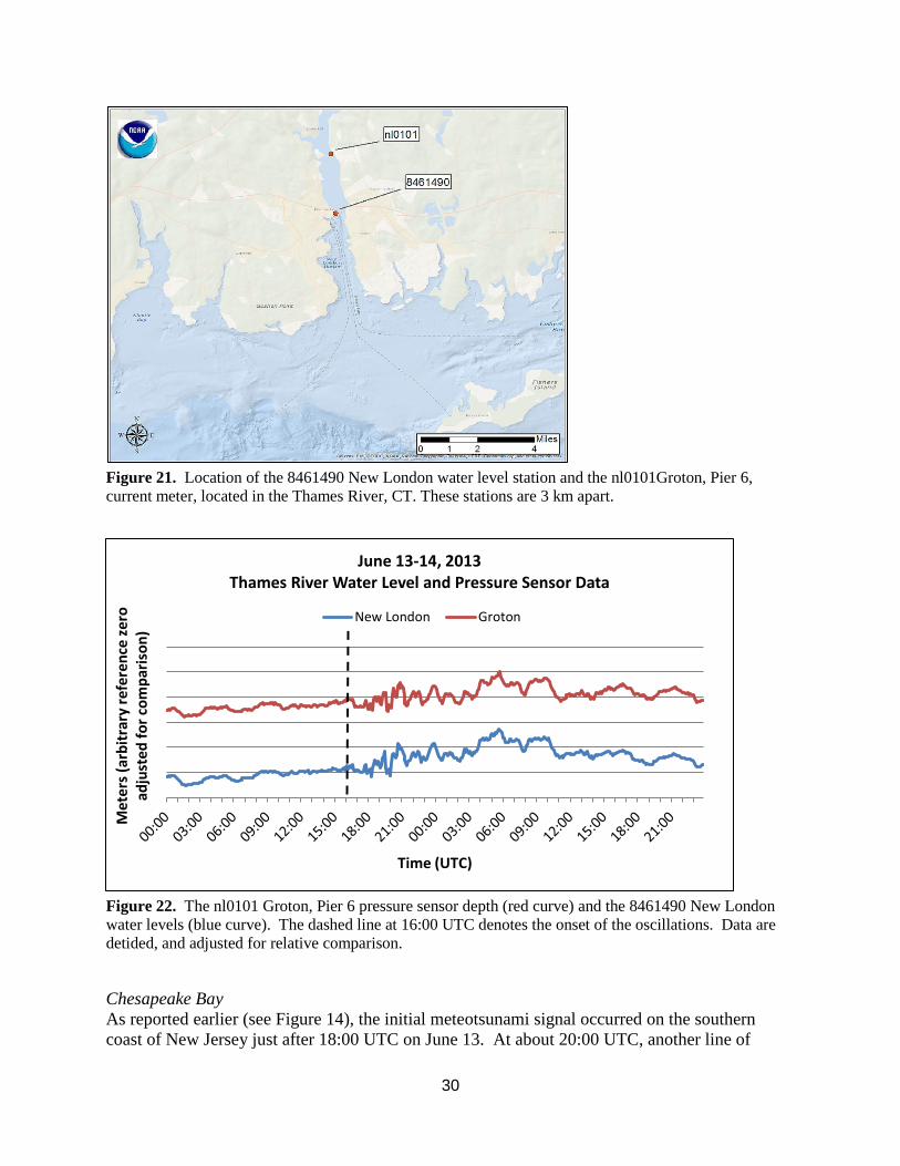
Figure 21. Location of the 8461490 New London water level station and the nl0101Groton, Pier 6, current meter, located in the Thames River, CT. These stations are 3 km apart.

Figure 22. The nl0101 Groton, Pier 6 pressure sensor depth (red curve) and the 8461490 New London water levels (blue curve). The dashed line at 16:00 UTC denotes the onset of the oscillations. Data are detided, and adjusted for relative comparison.

Chesapeake Bay As reported earlier (see Figure 14), the initial meteotsunami signal occurred on the southern coast of New Jersey just after 18:00 UTC on June 13. At about 20:00 UTC, another line of

Met

ers

(arb

itra

ry re

fere

nce

zero

ad

just

ed fo

r co

mpa

riso

n)

Time (UTC)

June 13-14, 2013 Thames River Water Level and Pressure Sensor Data

New London Groton

30

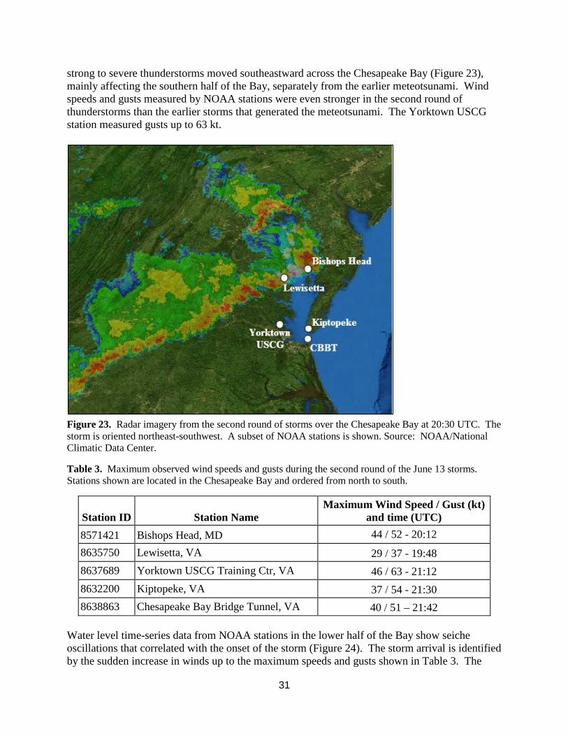
strong to severe thunderstorms moved southeastward across the Chesapeake Bay (Figure 23), mainly affecting the southern half of the Bay, separately from the earlier meteotsunami. Wind speeds and gusts measured by NOAA stations were even stronger in the second round of thunderstorms than the earlier storms that generated the meteotsunami. The Yorktown USCG station measured gusts up to 63 kt.

Figure 23. Radar imagery from the second round of storms over the Chesapeake Bay at 20:30 UTC. The storm is oriented northeast-southwest. A subset of NOAA stations is shown. Source: NOAA/National Climatic Data Center.

Table 3. Maximum observed wind speeds and gusts during the second round of the June 13 storms. Stations shown are located in the Chesapeake Bay and ordered from north to south.

Station ID Station Name Maximum Wind Speed / Gust (kt)

and time (UTC) 8571421 Bishops Head, MD 44 / 52 - 20:12 8635750 Lewisetta, VA 29 / 37 - 19:48 8637689 Yorktown USCG Training Ctr, VA 46 / 63 - 21:12 8632200 Kiptopeke, VA 37 / 54 - 21:30 8638863 Chesapeake Bay Bridge Tunnel, VA 40 / 51 – 21:42

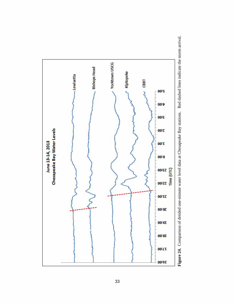
Water level time-series data from NOAA stations in the lower half of the Bay show seiche oscillations that correlated with the onset of the storm (Figure 24). The storm arrival is identified by the sudden increase in winds up to the maximum speeds and gusts shown in Table 3. The

31

southeastward progression of the storm can be clearly seen in the water level response, also marked by the red dashed lines in Figure 24.

32

Figu

re 2

4. C

ompa

rison

of d

etid

ed o

ne-m

inut

e w

ater

leve

l dat

a at

Che

sape

ake

Bay

stat

ions

. R

ed d

ashe

d lin

es in

dica

te th

e st

orm

arr

ival

.

33

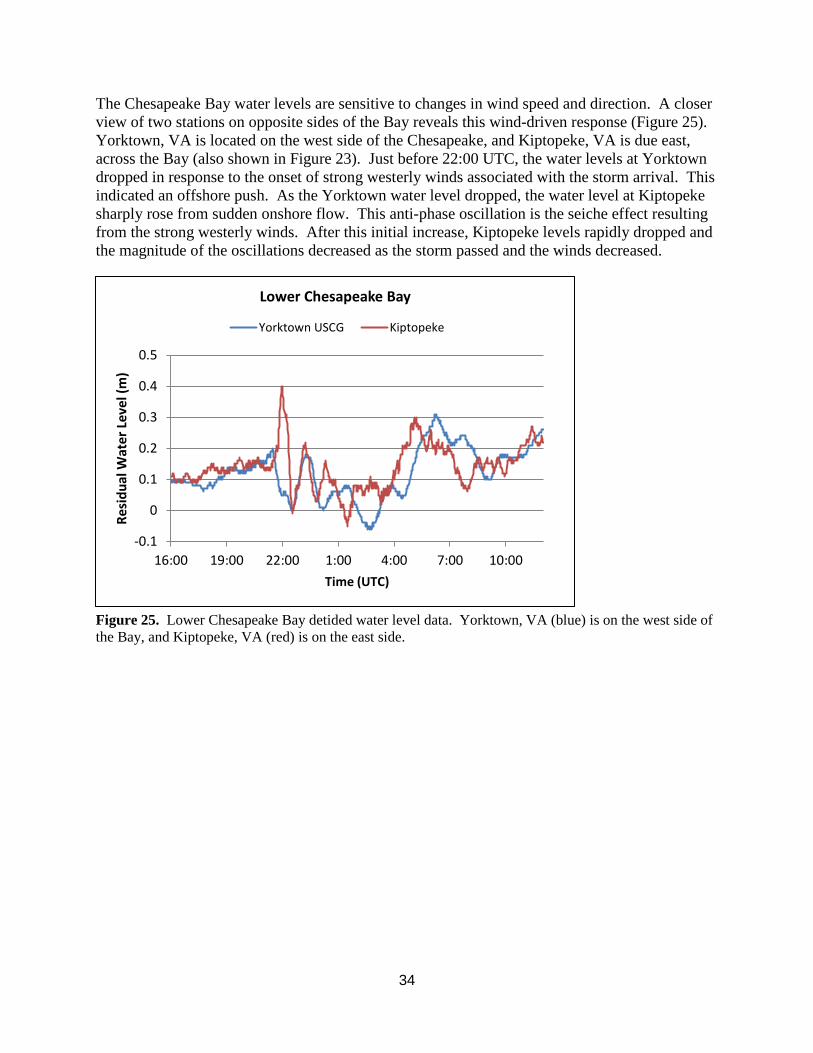
The Chesapeake Bay water levels are sensitive to changes in wind speed and direction. A closer view of two stations on opposite sides of the Bay reveals this wind-driven response (Figure 25). Yorktown, VA is located on the west side of the Chesapeake, and Kiptopeke, VA is due east, across the Bay (also shown in Figure 23). Just before 22:00 UTC, the water levels at Yorktown dropped in response to the onset of strong westerly winds associated with the storm arrival. This indicated an offshore push. As the Yorktown water level dropped, the water level at Kiptopeke sharply rose from sudden onshore flow. This anti-phase oscillation is the seiche effect resulting from the strong westerly winds. After this initial increase, Kiptopeke levels rapidly dropped and the magnitude of the oscillations decreased as the storm passed and the winds decreased.

Figure 25. Lower Chesapeake Bay detided water level data. Yorktown, VA (blue) is on the west side of the Bay, and Kiptopeke, VA (red) is on the east side.

-0.1

0

0.1

0.2

0.3

0.4

0.5

16:00 19:00 22:00 1:00 4:00 7:00 10:00

Resi

dual

Wat

er L

evel

(m)

Time (UTC)

Lower Chesapeake Bay

Yorktown USCG Kiptopeke

34

DISCUSSION

The June 2013 meteotsunami gained a lot of attention from the scientific community, since meteotsunamis have become more widely researched in recent years. There was a time lag between the storm and the incoming wave, and the direction of the storm was directly opposed to the wave it generated, which seems counter to traditional definitions of a meteotsunami. U.S. East Coast meteotsunamis are unique since they will not follow the typical setups and dynamics as described earlier in this report, where a pressure perturbation moves towards the shore and an associated amplified ocean wave moves in the same direction to cause the coastal inundation. The majority of U.S. East Coast weather systems flow eastward and offshore; however, as seen in the previous section, onshore atmospheric flows associated with typical meteotsunamis observed around the world are not required to create destructive waves along the U.S. coast. Similarly, Great Lakes events do not follow the classical definitions of meteotsunamis as determined from global events, since wind stress is a more prominent factor in wave magnitude.

The Atlantic Basin and wave dynamics

The Atlantic Basin is unique because a long ocean wave is impacted by the mid-Atlantic shelf break. The height of the forced wave moving offshore is depth-dependent, and a sudden drop in depth would generate free waves radiating outward. Wave reflection and refraction caused by bathymetric changes has been the subject of numerous studies in the Atlantic basin (Lipa 2013, Pasquet and Vilibić 2013, Mercer 2002, Vennell 2007, Vennell 2010). Pasquet and Vilibić (2013) examined data from several East Coast CO-OPS water level stations and focused on four meteotsunami events. In these four events, the storms that generated the long waves were moving offshore, similar to the 2013 event, and the waves were amplified from Proudman resonance. By comparing the time lag between the air pressure jump and the water level rise at the water level station, and the speed and direction of the atmospheric disturbance, they concluded that the water level oscillations measured at the coastal stations were due to reflected waves off the shelf break. In fact, they determined that minor meteotsunamis due to these reflected waves are relatively frequent along the East Coast, especially at Duck, NC. Mercer (2002) examined extreme oscillations that hit the coast of Newfoundland, Canada in 1999 and 2000, presumably caused by tropical storms passing nearby. The oscillations were not due to storm surge, since the storms were too far offshore for this wind-driven piling up of water to affect the shoreline. They used a numerical model to hypothesize that the storms generated ocean waves that reflected off changing bathymetry. These studies, plus further examination by NOAA (Knight et al. 2013, Wang et al. 2013) strongly suggest that shelf-edge reflection of the forced wave caused the coastal runup seen in the 2013 event.

Not all East Coast meteotsunami events are the result of storms moving offshore. On rare occasions, such as the 1992 Daytona Beach, FL event, alongshore or onshore atmospheric disturbances can cause catastrophic oscillations as well (Churchill 1995).

35

CONCLUSION

Tsunami awareness is vital for coastal communities, which are prone to inundation events. There is a lower probability of a seismic tsunami and its associated impacts on the East Coast compared to the West Coast, since rare submarine landslides are the primary potential source of East Coast tsunamis. However, the East Coast is more susceptible to meteotsunamis and the recent 2013 event reveals how extensive of an area can be impacted. Unfortunately, public awareness is not high since these events are usually minor or undetected by observers, and there hasn’t been much research into the generation and effects of East Coast meteotsunamis until recently. Detection of meteotsunamis is a concern because there is risk of a significant event causing injury or loss of life in addition to substantial property damage.

In some international regions, warning systems have been formally established. The Spanish Meteorological Office began forecasting meteotsunamis in 1984, and issued a “rissaga warning” the day before the catastrophic Ciutadella Harbor event. The warnings are qualitative, and based on forecast weather conditions that are conducive to triggering a meteotsunami in the area, as determined from past events and analyses (Jansa et al. 2007). Quantitative forecasting of wave amplitudes, however, is more difficult and is not operationally available. Renault et al. (2011) ran a regionally-nested ocean and atmosphere model to reproduce the conditions surrounding the 2006 Ciutadella Harbor meteotsunami. Strong sensitivity to the atmospheric initial boundary conditions, and bathymetry and coastline resolution created some bias between the model and observations, but the results were encouraging. Šepić and Vilibić (2011) also identify the requirements to develop and implement a real-time meteotsunami network for the Adriatic Sea, which involves focus on barometric pressure data, with the caveat that mean sea level preceding an event may also need to be considered.

Meteotsunami modeling and forecasting is a challenge. For the U.S. East Coast, the distinct conditions for the most common driver of meteotsunamis to occur require a perfect storm of variables that would generate a forced wave that reflects off the shelf break and travels at a particular speed and direction to affect the coastline. The NOAA-funded Meteotsunami Project, entitled “Towards a meteotsunami warning system along the U.S. coastline” (TMEWS) identified meteotsunami source characteristics with focus on recent events. The project results benefited subsequent modeling studies that employed existing tsunami models to simulate past meteotsunamis. For example, Whitmore and Knight (2014) used a tsunami forecast model coupled with a moving pressure perturbation to simulate the 2008 Boothbay event. Results from the TMEWS project and subsequent research show that establishing a forecasting system is possible. One advantage is that the source events that generate a meteotsunami can be forecasted whereas seismic events that generate a tsunami cannot. Therefore, meteotsunami warnings can be developed based on forecast conditions that are conducive to its generation. NOAA currently issues qualitative warnings through local Weather Forecast Offices (WFOs). Most recently, on June 4, 2014 a forecasted derecho was identified by NOAA as a possible trigger, and the NWS Weather Forecast Office in Mt. Holly, NJ included a warning in the Area Forecast Discussion of possible coastal surges. The storm became disorganized, however, so it did not result in a significant meteotsunami event.

Overall, successful prediction depends on a high-resolution forecast capable of resolving the pressure jumps (and wind speed jumps in the Great Lakes) that precede meteotsunami formation.

37

High-resolution forecasts (on the order of minutes) are needed; hourly forecasts will not suffice for this type of warning system. Similarly, high temporal resolution observations along the U.S. coastline as well as the open ocean are vital, especially since pressure jumps occur over minutes. NOAA one-minute water level data and six-minute meteorological data, NWS DART® buoys, and bathymetric data are key, along with digital elevation models. Lipa et al. (2013) illustrate the potential for HF radar observations to establish a half-hour warning for waves of similar height traveling over similar bathymetry to the 2013 event. The radars detected the 2013 meteotsunami 47 minutes before it arrived at the coast. In the meantime, NOAA will continue to issue qualitative warnings for meteotsunamis through WFOs.

38

ACKNOWLEDGEMENTS

We would like to thank CO-OPS colleagues Stephen Gill, Patrick Burke, and Adam Grodsky for their review and feedback on this report. We also thank Paul Whitmore, Eric Anderson, Nathan Becker, and Paul Huang for their constructive reviews and insightful feedback. Special thanks to Stephen Gill, who provided guidance and oversight. This report was prepared for publication by Brenda Via, CO-OPS.

39

REFERENCES

Akamatsu, H. (1978). Abikis in Nagasaki Harbor. In: The 100 Years of Nagasaki Marine Observatory. Nagasaki Marine Observatory, Nagasaki, pp. 154- 162.

Bechle, A. J., & Wu, C. H. The Lake Michigan meteotsunamis of 1954 revisited. Natural Hazards, 74(1), 1-23.

Churchill, D. D., Houston, S. H., & Bond, N. A. (1995). The Daytona Beach wave of 3-4 July 1992: A shallow-water gravity wave forced by a propagating squall line. Bulletin of the American Meteorological Society, 76(1), 21-32.

Donn, W. L. (1959). The Great Lakes storm surge of May 5, 1952. Journal of Geophysical Research, 64(2), 191-198.

Ewing, M., Press, F., & Donn, W. L. (1954). An explanation of the Lake Michigan wave of 26 June 1954. Science, 120 (3122), 684-686.

Fraser, D. (2013, June 15). Weather creates rare Cape Code tsunami. The Cape Code Times. Retrieved from http://www.capecodtimes.com.

Greenspan, H. P. (1956). The generation of edge waves by moving pressure distributions. Journal of Fluid Mechanics, 1(06), 574-592.

Hibiya, T., & Kajiura, K. (1982). Origin of the Abiki phenomenon (a kind of seiche) in Nagasaki Bay. Journal of the Oceanographical Society of Japan, 38(3), 172-182.

Honda, K., Terada, T., Yoshida, Y., & Isitani, D. (1908). An investigation on the secondary undulations of oceanic tides. J. College Sci., Imper. Univ. Tokyo, 108 p.

Hughes, L. A. (1965). The prediction of surges in the southern basin of Lake Michigan Part 111. The Operational Basis for Prediction. Monthly Weather Review, 93, 292-296.

Jansa, A., Monserrat, S., & Gomis, D. (2007). The rissaga of 15 June 2006 in Ciutadella (Menorca), a meteorological tsunami. Advances in Geosciences, 12, 1-4.

Knight, W. R., Whitmore, P., Kim, Y., Wang, D., Becker, N. C., Weinstein, S., & Walker, K. (2013, December). The US East Coast Meteotsunami of June 13, 2013. In AGU Fall Meeting Abstracts (Vol. 1, p. 1740).

Lipa, B., Parikh, H., Barrick, D., Roarty, H., & Glenn, S. (2013). High-frequency radar observations of the June 2013 US East Coast meteotsunami. Natural Hazards, 74(1), 1-14.

Mercer, D., Sheng, J., Greatbatch, R. J., & Bobanović, J. (2002). Barotropic waves generated by storms moving rapidly over shallow water. Journal of Geophysical Research: Oceans (1978–2012), 107(C10), 16-1.

40

Monserrat, S., Ramis, C., & Thorpe, A.J. (1991). Large‐amplitude pressure oscillations in the western Mediterranean. Geophysical Research Letters: 18(2), 183-186.

Monserrat, S., Vilibić, I., & Rabinovich, A. B. (2006). Meteotsunamis: atmospherically induced destructive ocean waves in the tsunami frequency band. Natural Hazards and Earth System Science, 6(6), 1035-1051.

Nakano, M., & Unoki, S. (1962): On the seiches (the secondary undulations of tides) along the coasts of Japan. Records of Oceanographic Works in Japan, Special Number 6, 169–214.

National Geophysical Data Center / World Data Service (NGDC/WDS): Global Historical Tsunami Database. National Geophysical Data Center, NOAA. doi:10.7289/V5PN93H7 [June 10, 2014]

Pasquet, S., & Vilibić, I. (2013). Shelf edge reflection of atmospherically generated long ocean waves along the central US East Coast. Continental Shelf Research, 66, 1-8.

Proudman, J. (1929). The Effects on the Sea of Changes in Atmospheric Pressure. Geophysical Journal International, 2(s4), 197-209.

Rabinovich, A. B. (2009). Seiches and harbour oscillations. Handbook of coastal and ocean engineering, 193-236.

Renault, L., Vizoso, G., Jansá, A., Wilkin, J., & Tintoré, J. (2011). Toward the predictability of meteotsunamis in the Balearic Sea using regional nested atmosphere and ocean models. Geophysical Research Letters, 38(10).

Sallenger Jr, A. H., List, J. H., Gelfenbaum, G., Stumpf, R. P., & Hansen, M. (1995). Large wave at Daytona Beach, Florida, explained as a squall-line surge. Journal of Coastal Research, 1383-1388.

Šepić, J., & Rabinovich, A. B. (2014). Meteotsunami in the Great Lakes and on the Atlantic coast of the United States generated by the “derecho” of June 29–30, 2012. Natural Hazards, 74(1), 75-107.

Šepić, J., & Vilibić, I. (2011). The development and implementation of a real-time meteotsunami warning network for the Adriatic Sea. Natural Hazards and Earth System Science, 11(1), 83-91.

"Tsunami of 13 June, 2013 (Northwestern Atlantic Ocean)," National Tsunami Warning Center, National Oceanic and Atmospheric Administration/National Weather Service, Retrieved from http://ntwc.arh.noaa.gov/previous.events/?p=06-13-13.

Vennell, R. (2007). Long barotropic waves generated by a storm crossing topography. Journal of Physical Oceanography, 37(12), 2809-2823.

41

Vennell, R. (2010). Resonance and trapping of topographic transient ocean waves generated by a moving atmospheric disturbance. Journal of Fluid Mechanics, 650, 427-442.

Vilibić, I. (2008). Numerical simulations of the Proudman resonance. Continental Shelf Research, 28(4), 574-581.

Vilibić, I., Horvath, K., Mahović, N. S., Monserrat, S., Marcos, M., Amores, A., & Fine, I. (2014). Atmospheric processes responsible for generation of the 2008 Boothbay meteotsunami. Natural Hazards, 74(1), 1-29.

Wang, D., Becker N.C., Weinstein, S., Whitmore, P., Knight, W., Kim, Y., Bouchard, R.H., & Grissom, K. (2013, December). June 13, 2013 US East Coast Meteotsunami: Comparing a Numerical Model With Observations. In AGU Fall Meeting Abstracts (Vol. 1, p. 02).

Whitmore, P., & Knight, B. Meteotsunami forecasting: sensitivities demonstrated by the 2008 Boothbay, Maine, event. Natural Hazards, 74(1), 1-13.

42