nips2010: optimization algorithms in machine learning

Optimization Algorithms in Machine Learning

Stephen Wright

University of Wisconsin-Madison

NIPS Tutorial, 6 Dec 2010

Stephen Wright (UW-Madison) Optimization in Machine Learning NIPS Tutorial, 6 Dec 2010 1 / 82

Optimization

Optimization is going through a period of growth and revitalization,driven largely by new applications in many areas.

Standard paradigms (LP, QP, NLP, MIP) are still important, alongwith general-purpose software, enabled by modeling languages thatmake the software easier to use.

However, there is a growing emphasis on “picking and choosing”algorithmic elements to fit the characteristics of a given application— building up a suitable algorithm from a “toolkit” of components.

It’s more important than ever to understand the fundamentals ofalgorithms as well as the demands of the application, so that goodchoices are made in matching algorithms to applications.

We present a selection of algorithmic fundamentals in this tutorial, with anemphasis on those of current and potential interest in machine learning.


Topics

I. First-order Methods

II. Stochastic and Incremental Gradient Methods

III. Shrinking/Thresholding for Regularized Formulations

IV. Optimal Manifold Identification and Higher-Order Methods.

V. Decomposition and Coordinate Relaxation


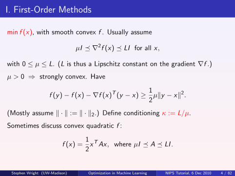
I. First-Order Methods

min f (x), with smooth convex f . Usually assume

µI ∇2f (x) LI for all x ,

with 0 ≤ µ ≤ L. (L is thus a Lipschitz constant on the gradient ∇f .)

µ > 0 ⇒ strongly convex. Have

f (y)− f (x)−∇f (x)T (y − x) ≥ 1

2µ‖y − x‖2.

(Mostly assume ‖ · ‖ := ‖ · ‖2.) Define conditioning κ := L/µ.

Sometimes discuss convex quadratic f :

f (x) =1

2xTAx , where µI A LI .


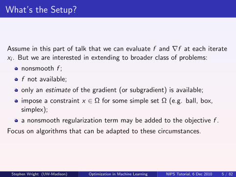
What’s the Setup?

Assume in this part of talk that we can evaluate f and ∇f at each iteratexi . But we are interested in extending to broader class of problems:

nonsmooth f ;

f not available;

only an estimate of the gradient (or subgradient) is available;

impose a constraint x ∈ Ω for some simple set Ω (e.g. ball, box,simplex);

a nonsmooth regularization term may be added to the objective f .

Focus on algorithms that can be adapted to these circumstances.


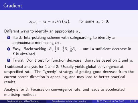
Gradient

xk+1 = xk − αk∇f (xk), for some αk > 0.

Different ways to identify an appropriate αk .

1 Hard: Interpolating scheme with safeguarding to identify anapproximate minimizing αk .

2 Easy: Backtracking. α, 12 α, 1

4 α, 18 α, ... until a sufficient decrease in

f is obtained.

3 Trivial: Don’t test for function decrease. Use rules based on L and µ.

Traditional analysis for 1 and 2: Usually yields global convergence atunspecified rate. The “greedy” strategy of getting good decrease from thecurrent search direction is appealing, and may lead to better practicalresults.

Analysis for 3: Focuses on convergence rate, and leads to acceleratedmultistep methods.


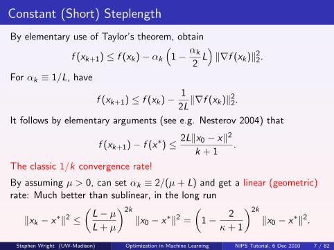
Constant (Short) Steplength

By elementary use of Taylor’s theorem, obtain

f (xk+1) ≤ f (xk)− αk

(1− αk

2L)‖∇f (xk)‖2

2.

For αk ≡ 1/L, have

f (xk+1) ≤ f (xk)− 1

2L‖∇f (xk)‖2

2.

It follows by elementary arguments (see e.g. Nesterov 2004) that

f (xk+1)− f (x∗) ≤ 2L‖x0 − x‖2

k + 1.

The classic 1/k convergence rate!

By assuming µ > 0, can set αk ≡ 2/(µ+ L) and get a linear (geometric)rate: Much better than sublinear, in the long run

‖xk − x∗‖2 ≤(

L− µL + µ

)2k

‖x0 − x∗‖2 =

(1− 2

κ+ 1

)2k

‖x0 − x∗‖2.


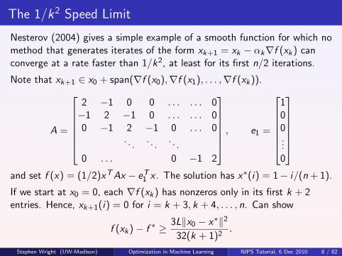
The 1/k2 Speed Limit

Nesterov (2004) gives a simple example of a smooth function for which nomethod that generates iterates of the form xk+1 = xk − αk∇f (xk) canconverge at a rate faster than 1/k2, at least for its first n/2 iterations.

Note that xk+1 ∈ x0 + span(∇f (x0),∇f (x1), . . . ,∇f (xk)).

A =

2 −1 0 0 . . . . . . 0−1 2 −1 0 . . . . . . 00 −1 2 −1 0 . . . 0

. . .. . .

. . .

0 . . . 0 −1 2

, e1 =

100...0

and set f (x) = (1/2)xTAx − eT1 x . The solution has x∗(i) = 1− i/(n + 1).

If we start at x0 = 0, each ∇f (xk) has nonzeros only in its first k + 2entries. Hence, xk+1(i) = 0 for i = k + 3, k + 4, . . . , n. Can show

f (xk)− f ∗ ≥ 3L‖x0 − x∗‖2

32(k + 1)2.


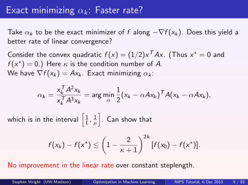
Exact minimizing αk : Faster rate?

Take αk to be the exact minimizer of f along −∇f (xk). Does this yield abetter rate of linear convergence?

Consider the convex quadratic f (x) = (1/2)xTAx . (Thus x∗ = 0 andf (x∗) = 0.) Here κ is the condition number of A.We have ∇f (xk) = Axk . Exact minimizing αk :

αk =xTk A2xk

xTk A3xk

= arg minα

1

2(xk − αAxk)TA(xk − αAxk),

which is in the interval[

1L ,

1µ

]. Can show that

f (xk)− f (x∗) ≤(

1− 2

κ+ 1

)2k

[f (x0)− f (x∗)].

No improvement in the linear rate over constant steplength.


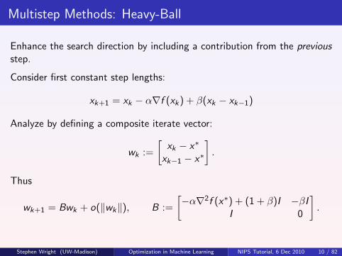
Multistep Methods: Heavy-Ball

Enhance the search direction by including a contribution from the previousstep.

Consider first constant step lengths:

xk+1 = xk − α∇f (xk) + β(xk − xk−1)

Analyze by defining a composite iterate vector:

wk :=

[xk − x∗

xk−1 − x∗

].

Thus

wk+1 = Bwk + o(‖wk‖), B :=

[−α∇2f (x∗) + (1 + β)I −βI

I 0

].


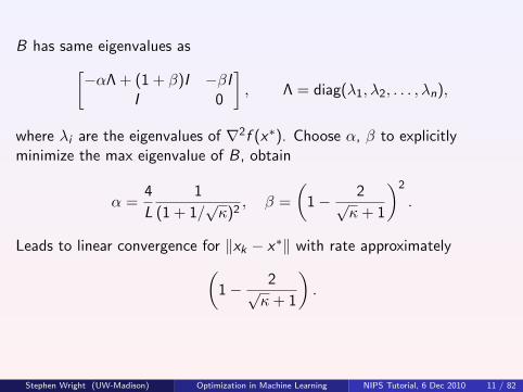
B has same eigenvalues as[−αΛ + (1 + β)I −βI

I 0

], Λ = diag(λ1, λ2, . . . , λn),

where λi are the eigenvalues of ∇2f (x∗). Choose α, β to explicitlyminimize the max eigenvalue of B, obtain

α =4

L

1

(1 + 1/√κ)2

, β =

(1− 2√

κ+ 1

)2

.

Leads to linear convergence for ‖xk − x∗‖ with rate approximately(1− 2√

κ+ 1

).


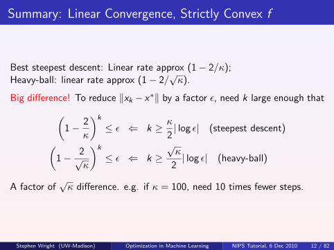
Summary: Linear Convergence, Strictly Convex f

Best steepest descent: Linear rate approx (1− 2/κ);Heavy-ball: linear rate approx (1− 2/

√κ).

Big difference! To reduce ‖xk − x∗‖ by a factor ε, need k large enough that(1− 2

κ

)k

≤ ε ⇐ k ≥ κ

2| log ε| (steepest descent)(

1− 2√κ

)k

≤ ε ⇐ k ≥√κ

2| log ε| (heavy-ball)

A factor of√κ difference. e.g. if κ = 100, need 10 times fewer steps.


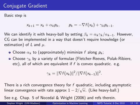
Conjugate Gradient

Basic step is

xk+1 = xk + αkpk , pk = −∇f (xk) + γkpk−1.

We can identify it with heavy-ball by setting βk = αkγk/αk−1. However,CG can be implemented in a way that doesn’t require knowledge (orestimation) of L and µ.

Choose αk to (approximately) miminize f along pk ;

Choose γk by a variety of formulae (Fletcher-Reeves, Polak-Ribiere,etc), all of which are equivalent if f is convex quadratic. e.g.

γk = ‖∇f (xk)‖2/‖∇f (xk−1)‖2.

There is a rich convergence theory for f quadratic, including asymptoticlinear convergence with rate approx 1− 2/

√κ. (Like heavy-ball.)

See e.g. Chap. 5 of Nocedal & Wright (2006) and refs therein.Stephen Wright (UW-Madison) Optimization in Machine Learning NIPS Tutorial, 6 Dec 2010 13 / 82

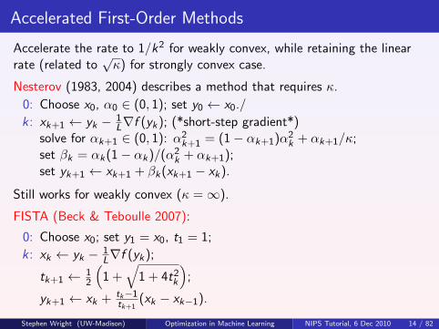
Accelerated First-Order Methods

Accelerate the rate to 1/k2 for weakly convex, while retaining the linearrate (related to

√κ) for strongly convex case.

Nesterov (1983, 2004) describes a method that requires κ.

0: Choose x0, α0 ∈ (0, 1); set y0 ← x0./

k : xk+1 ← yk − 1L∇f (yk); (*short-step gradient*)

solve for αk+1 ∈ (0, 1): α2k+1 = (1− αk+1)α2

k + αk+1/κ;set βk = αk(1− αk)/(α2

k + αk+1);set yk+1 ← xk+1 + βk(xk+1 − xk).

Still works for weakly convex (κ =∞).

FISTA (Beck & Teboulle 2007):

0: Choose x0; set y1 = x0, t1 = 1;

k: xk ← yk − 1L∇f (yk);

tk+1 ← 12

(1 +

√1 + 4t2

k

);

yk+1 ← xk + tk−1tk+1

(xk − xk−1).


k

xk+1

xk

yk+1

xk+2

yk+2

y


Convergence Results: Nesterov

If α0 ≥ 1/√κ, have

f (xk)− f (x∗) ≤ c1 min

((1− 1√

κ

)k

,4L

(√

L + c2k)2

),

where constants c1 and c2 depend on x0, α0, L.

Linear convergence at “heavy-ball” rate in strongly convex case, otherwise1/k2. FISTA also achieves 1/k2 rate.

Analysis: Not intuitive. Based on bounding the difference between f and aquadratic approximation to it, at x∗. FISTA analysis is 2-3 pages.


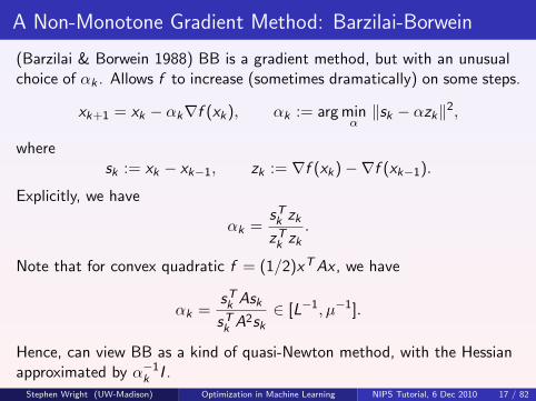
A Non-Monotone Gradient Method: Barzilai-Borwein

(Barzilai & Borwein 1988) BB is a gradient method, but with an unusualchoice of αk . Allows f to increase (sometimes dramatically) on some steps.

xk+1 = xk − αk∇f (xk), αk := arg minα‖sk − αzk‖2,

wheresk := xk − xk−1, zk := ∇f (xk)−∇f (xk−1).

Explicitly, we have

αk =sTk zk

zTk zk

.

Note that for convex quadratic f = (1/2)xTAx , we have

αk =sTk Ask

sTk A2sk∈ [L−1, µ−1].

Hence, can view BB as a kind of quasi-Newton method, with the Hessianapproximated by α−1

k I .Stephen Wright (UW-Madison) Optimization in Machine Learning NIPS Tutorial, 6 Dec 2010 17 / 82

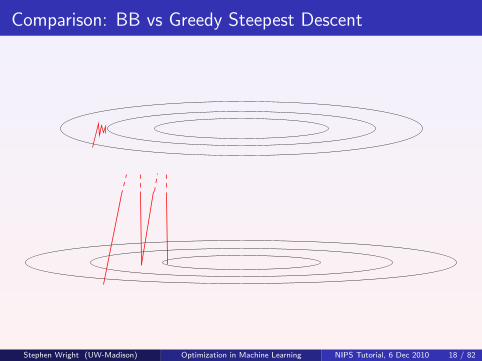
Comparison: BB vs Greedy Steepest Descent


Many BB Variants

can use αk = sTk sk/sTk zk in place of αk = sTk zk/zTk zk ;

alternate between these two formulae;

calculate αk as above and hold it constant for 2, 3, or 5 successivesteps;

take αk to be the exact steepest descent step from the previousiteration.

Nonmonotonicity appears essential to performance. Some variants getglobal convergence by requiring a sufficient decrease in f over the worst ofthe last 10 iterates.

The original 1988 analysis in BB’s paper is nonstandard and illuminating(just for a 2-variable quadratic).

In fact, most analyses of BB and related methods are nonstandard, andconsider only special cases. The precursor of such analyses is Akaike(1959). More recently, see Ascher, Dai, Fletcher, Hager and others.


Primal-Dual Averaging

(see Nesterov 2009) Basic step:

xk+1 = arg minx

1

k + 1

k∑i=0

[f (xi ) +∇f (xi )T (x − xi )] +

γ√k‖x − x0‖2

= arg minx

gTk x +

γ√k‖x − x0‖2,

where gk :=∑k

i=0∇f (xi )/(k + 1) — the averaged gradient.

The last term is always centered at the first iterate x0.

Gradient information is averaged over all steps, with equal weights.

γ is constant - results can be sensitive to this value.

The approach still works for convex nondifferentiable f , where ∇f (xi )is replaced by a vector from the subgradient ∂f (xi ).


Convergence Properties

Nesterov proves convergence for averaged iterates:

xk+1 =1

k + 1

k∑i=0

xi .

Provided the iterates and the solution x∗ lie within some ball of radius Daround x0, we have

f (xk+1)− f (x∗) ≤ C√k,

where C depends on D, a uniform bound on ‖∇f (x)‖, and γ (coefficientof stabilizing term).

Note: There’s averaging in both primal (xi ) and dual (∇f (xi )) spaces.

Generalizes easily and robustly to the case in which only estimatedgradients or subgradients are available.

(Averaging smooths the errors in the individual gradient estimates.)


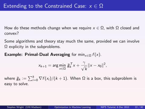
Extending to the Constrained Case: x ∈ Ω

How do these methods change when we require x ∈ Ω, with Ω closed andconvex?

Some algorithms and theory stay much the same, provided we can involveΩ explicity in the subproblems.

Example: Primal-Dual Averaging for minx∈Ω f (x).

xk+1 = arg minx∈Ω

gTk x +

γ√k‖x − x0‖2,

where gk :=∑k

i=0∇f (xi )/(k + 1). When Ω is a box, this subproblem iseasy to solve.


Example: Nesterov’s Constant Step Scheme for minx∈Ω f (x). Requiresjust only calculation to be changed from the unconstrained version.

0: Choose x0, α0 ∈ (0, 1); set y0 ← x0, q ← 1/κ = µ/L.

k : xk+1 ← arg miny∈Ω12‖y − [yk − 1

L∇f (yk)]‖22;

solve for αk+1 ∈ (0, 1): α2k+1 = (1− αk+1)α2

k + qαk+1;set βk = αk(1− αk)/(α2

k + αk+1);set yk+1 ← xk+1 + βk(xk+1 − xk).

Convergence theory is unchanged.


Regularized Optimization (More Later)

FISTA can be applied with minimal changes to the regularized problem

minx

f (x) + τψ(x),

where f is convex and smooth, ψ convex and “simple” but usuallynonsmooth, and τ is a positive parameter.

Simply replace the gradient step by

xk = arg minx

L

2

∥∥∥∥x −[

yk −1

L∇f (yk)

]∥∥∥∥2

+ τψ(x).

(This is the “shrinkage” step; when ψ ≡ 0 or ψ = ‖ · ‖1, can be solvedcheaply.)

More on this later.


Further Reading

1 Y. Nesterov, Introductory Lectures on Convex Optimization: A Basic Course,Kluwer Academic Publishers, 2004.

2 A. Beck and M. Teboulle, “Gradient-based methods with application to signalrecovery problems,” in press, 2010. (See Teboulle’s web site).

3 B. T. Polyak, Introduction to Optimization, Optimization Software Inc, 1987.

4 J. Barzilai and J. M. Borwein, “Two-point step size gradient methods,” IMAJournal of Numerical Analysis, 8, pp. 141-148, 1988.

5 Y. Nesterov, “Primal-dual subgradient methods for convex programs,”Mathematical Programming, Series B, 120, pp. 221-259, 2009.


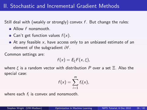
II. Stochastic and Incremental Gradient Methods

Still deal with (weakly or strongly) convex f . But change the rules:

Allow f nonsmooth.

Can’t get function values f (x).

At any feasible x , have access only to an unbiased estimate of anelement of the subgradient ∂f .

Common settings are:f (x) = EξF (x , ξ),

where ξ is a random vector with distribution P over a set Ξ. Also thespecial case:

f (x) =m∑i=1

fi (x),

where each fi is convex and nonsmooth.


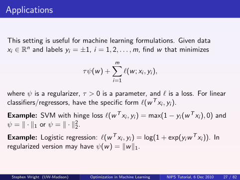
Applications

This setting is useful for machine learning formulations. Given dataxi ∈ Rn and labels yi = ±1, i = 1, 2, . . . ,m, find w that minimizes

τψ(w) +m∑i=1

`(w ; xi , yi ),

where ψ is a regularizer, τ > 0 is a parameter, and ` is a loss. For linearclassifiers/regressors, have the specific form `(wT xi , yi ).

Example: SVM with hinge loss `(wT xi , yi ) = max(1− yi (wT xi ), 0) andψ = ‖ · ‖1 or ψ = ‖ · ‖2

2.

Example: Logistic regression: `(wT xi , yi ) = log(1 + exp(yiwT xi )). In

regularized version may have ψ(w) = ‖w‖1.


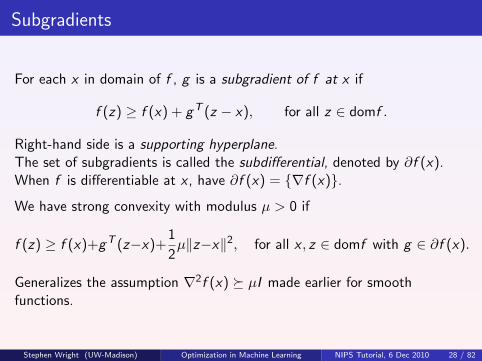
Subgradients

For each x in domain of f , g is a subgradient of f at x if

f (z) ≥ f (x) + gT (z − x), for all z ∈ domf .

Right-hand side is a supporting hyperplane.The set of subgradients is called the subdifferential, denoted by ∂f (x).When f is differentiable at x , have ∂f (x) = ∇f (x).

We have strong convexity with modulus µ > 0 if

f (z) ≥ f (x)+gT (z−x)+1

2µ‖z−x‖2, for all x , z ∈ domf with g ∈ ∂f (x).

Generalizes the assumption ∇2f (x) µI made earlier for smoothfunctions.


x

supporting hyperplanes

f


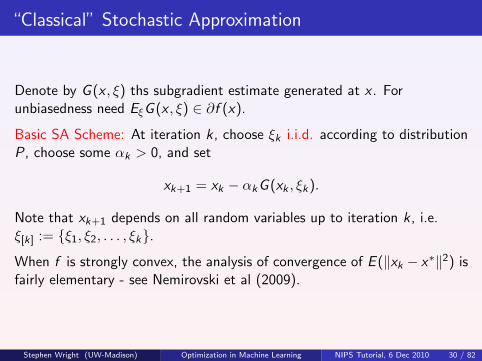
“Classical” Stochastic Approximation

Denote by G (x , ξ) ths subgradient estimate generated at x . Forunbiasedness need EξG (x , ξ) ∈ ∂f (x).

Basic SA Scheme: At iteration k, choose ξk i.i.d. according to distributionP, choose some αk > 0, and set

xk+1 = xk − αkG (xk , ξk).

Note that xk+1 depends on all random variables up to iteration k , i.e.ξ[k] := ξ1, ξ2, . . . , ξk.

When f is strongly convex, the analysis of convergence of E (‖xk − x∗‖2) isfairly elementary - see Nemirovski et al (2009).


Rate: 1/k

Define ak = 12 E (‖xk − x∗‖2). Assume there is M > 0 such that

E (‖G (x , ξ)‖2) ≤ M2 for all x of interest. Thus

1

2‖xk+1 − x∗‖2

2

=1

2‖xk − αkG (xk , ξk)− x∗‖2

=1

2‖xk − x∗‖2

2 − αk(xk − x∗)TG (xk , ξk) +1

2α2k‖G (xk , ξk)‖2.

Taking expectations, get

ak+1 ≤ ak − αkE [(xk − x∗)TG (xk , ξk)] +1

2α2kM2.

For middle term, have

E [(xk − x∗)TG (xk , ξk)] = Eξ[k−1]Eξk [(xk − x∗)TG (xk , ξk)|ξ[k−1]]

= Eξ[k−1](xk − x∗)Tgk ,


... wheregk := Eξk [G (xk , ξk)|ξ[k−1]] ∈ ∂f (xk).

By strong convexity, have

(xk − x∗)Tgk ≥ f (xk)− f (x∗) +1

2µ‖xk − x∗‖2 ≥ µ‖xk − x∗‖2.

Hence by taking expectations, we get E [(xk − x∗)Tgk ] ≥ 2µak . Then,substituting above, we obtain

ak+1 ≤ (1− 2µαk)ak +1

2α2kM2

When

αk ≡1

kµ,

a neat inductive argument (exercise!) reveals the 1/k rate:

ak ≤Q

2k, for Q := max

(‖x1 − x∗‖2,

M2

µ2

).


But... What if we don’t know µ? Or if µ = 0?

The choice αk = 1/(kµ) requires strong convexity, with knowledge of themodulus µ. An underestimate of µ can greatly degrade the performance ofthe method (see example in Nemirovski et al. 2009).

Now describe a Robust Stochastic Approximation approach, which has arate 1/

√k (in function value convergence), and works for weakly convex

nonsmooth functions and is not sensitive to choice of parameters in thestep length.

This is the approach that generalizes to mirror descent.


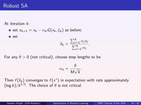
Robust SA

At iteration k :

set xk+1 = xk − αkG (xk , ξk) as before;

set

xk =

∑ki=1 αixi∑ki=1 αi

.

For any θ > 0 (not critical), choose step lengths to be

αk =θ

M√

k.

Then f (xk) converges to f (x∗) in expectation with rate approximately(log k)/k1/2. The choice of θ is not critical.


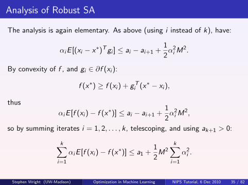
Analysis of Robust SA

The analysis is again elementary. As above (using i instead of k), have:

αiE [(xi − x∗)Tgi ] ≤ ai − ai+1 +1

2α2i M2.

By convexity of f , and gi ∈ ∂f (xi ):

f (x∗) ≥ f (xi ) + gTi (x∗ − xi ),

thus

αiE [f (xi )− f (x∗)] ≤ ai − ai+1 +1

2α2i M2,

so by summing iterates i = 1, 2, . . . , k , telescoping, and using ak+1 > 0:

k∑i=1

αiE [f (xi )− f (x∗)] ≤ a1 +1

2M2

k∑i=1

α2i .


Thus dividing by∑

i=1 αi :

E

[∑ki=1 αi f (xi )∑k

i=1 αi

− f (x∗)

]≤

a1 + 12 M2

∑ki=1 α

2i∑k

i=1 αi

.

By convexity, we have

f (xk) ≤∑k

i=1 αi f (xi )∑ki=1 αi

,

so obtain the fundamental bound:

E [f (xk)− f (x∗)] ≤a1 + 1

2 M2∑k

i=1 α2i∑k

i=1 αi

.


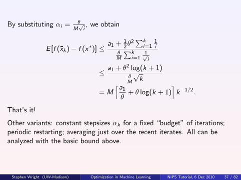
By substituting αi = θM√i, we obtain

E [f (xk)− f (x∗)] ≤a1 + 1

2θ2∑k

i=11i

θM

∑ki=1

1√i

≤ a1 + θ2 log(k + 1)θM

√k

= M[a1

θ+ θ log(k + 1)

]k−1/2.

That’s it!

Other variants: constant stepsizes αk for a fixed “budget” of iterations;periodic restarting; averaging just over the recent iterates. All can beanalyzed with the basic bound above.


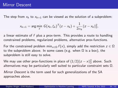
Mirror Descent

The step from xk to xk+1 can be viewed as the solution of a subproblem:

xk+1 = arg minz

G (xk , ξk)T (z − xk) +1

2αk‖z − xk‖2

2,

a linear estimate of f plus a prox-term. This provides a route to handlingconstrained problems, regularized problems, alternative prox-functions.

For the constrained problem minx∈Ω f (x), simply add the restriction z ∈ Ωto the subproblem above. In some cases (e.g. when Ω is a box), thesubproblem is still easy to solve.

We may use other prox-functions in place of (1/2)‖z − x‖22 above. Such

alternatives may be particularly well suited to particular constraint sets Ω.

Mirror Descent is the term used for such generalizations of the SAapproaches above.


Mirror Descent cont’d

Given constraint set Ω, choose a norm ‖ · ‖ (not necessarily Euclidean).Define the distance-generating function ω to be a strongly convex functionon Ω with modulus 1 with respect to ‖ · ‖, that is,

(ω′(x)− ω′(z))T (x − z) ≥ ‖x − z‖2, for all x , z ∈ Ω,

where ω′(·) denotes an element of the subdifferential.

Now define the prox-function V (x , z) as follows:

V (x , z) = ω(z)− ω(x)− ω′(x)T (z − x).

This is also known as the Bregman distance. We can use it in thesubproblem in place of 1

2‖ · ‖2:

xk+1 = arg minz∈Ω

G (xk , ξk)T (z − xk) +1

αkV (z , xk).


Bregman distance is the deviation from linearity:

ω

x z

V(x,z)


Bregman Distances: Examples

For any Ω, we can use ω(x) := (1/2)‖x − x‖22, leading to prox-function

V (x , z) = (1/2)‖x − z‖22.

For the simplex Ω = x ∈ Rn : x ≥ 0,∑n

i=1 xi = 1, we can use insteadthe 1-norm ‖ · ‖1, choose ω to be the entropy function

ω(x) =n∑

i=1

xi log xi ,

leading to Bregman distance

V (x , z) =n∑

i=1

zi log(zi/xi ).

These are the two most useful cases.

Convergence results for SA can be generalized to mirror descent.


Incremental Gradient

(See e.g. Bertsekas (2011) and references therein.) Finite sums:

f (x) =m∑i=1

fi (x).

Step k typically requires choice of one index ik ∈ 1, 2, . . . ,m andevaluation of ∇fik (xk). Components ik are selected sometimes randomly orcyclically. (Latter option does not exist in the setting f (x) := EξF (x ; ξ).)

There are incremental versions of the heavy-ball method:

xk+1 = xk − αk∇fik (xk) + β(xk − xk−1).

Approach like dual averaging: assume a cyclic choice of ik , andapproximate ∇f (xk) by the average of ∇fi (x) over the last m iterates:

xk+1 = xk −αk

m

m∑l=1

∇fik−l+1(xk−l+1).


Achievable Accuracy

Consider the basic incremental method:

xk+1 = xk − αk∇fik (xk).

How close can f (xk) come to f (x∗) — deterministically (not just inexpectation).

Bertsekas (2011) obtains results for constant steps αk ≡ α.

cyclic choice of ik : lim infk→∞

f (xk) ≤ f (x∗) + αβm2c2.

random choice of ik : lim infk→∞

f (xk) ≤ f (x∗) + αβmc2.

where β is close to 1 and c is a bound on the Lipschitz constants for ∇fi .

(Bertsekas actually proves these results in the more general context ofregularized optimization - see below.)


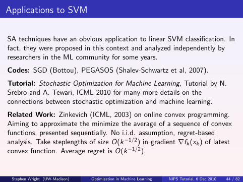
Applications to SVM

SA techniques have an obvious application to linear SVM classification. Infact, they were proposed in this context and analyzed independently byresearchers in the ML community for some years.

Codes: SGD (Bottou), PEGASOS (Shalev-Schwartz et al, 2007).

Tutorial: Stochastic Optimization for Machine Learning, Tutorial by N.Srebro and A. Tewari, ICML 2010 for many more details on theconnections between stochastic optimization and machine learning.

Related Work: Zinkevich (ICML, 2003) on online convex programming.Aiming to approximate the minimize the average of a sequence of convexfunctions, presented sequentially. No i.i.d. assumption, regret-basedanalysis. Take steplengths of size O(k−1/2) in gradient ∇fk(xk) of latestconvex function. Average regret is O(k−1/2).


Further Reading

1 A. Nemirovski, A. Juditsky, G. Lan, and A. Shapiro, “Robust stochasticapproximation approach to stochastic programming,” SIAM Journal onOptimization, 19, pp. 1574-1609, 2009.

2 D. P. Bertsekas, “Incremental gradient, subgradient, and proximal methods forconvex optimization: A Survey,” Chapter 4 in Optimization and Machine Learning,upcoming volume edited by S. Nowozin, S. Sra, and S. J. Wright (2011).

3 A. Juditsky and A. Nemirovski, “ First-order methods for nonsmooth convexlarge-scale optimization. I: General-purpose methods,” Chapter 5 in Optimizationand Machine Learning (2011).

4 A. Juditsky and A. Nemirovski, “ First-order methods for nonsmooth convexlarge-scale optimization. I: Utilizing problem structure,” Chapter 6 in Optimizationand Machine Learning (2011).

5 O. L. Mangasarian and M. Solodov, “Serial and parallel backpropagationconvergencevia nonmonotone perturbed minimization,” Optimization Methods andSoftware 4 (1994), pp. 103–116.

6 D. Blatt, A. O. Hero, and H. Gauchman, “A convergent incremental gradientmethod with constant step size,” SIAM Journal on Optimization 18 (2008), pp.29–51.


III. Shrinking/Thresholding for Regularized Optimization

In many applications, we seek not an exact minimizer of the underlyingobjective, but rather an approximate minimizer that satisfies certaindesirable properties:

sparsity (few nonzeros);

low-rank (if a matrix);

low “total-variation”;

generalizability. (Vapnik: “...tradeoff between the quality of theapproximation of the given data and the complexity of theapproximating function.”)

“Desirable” properties depend on context and application .

A common way to obtain structured solutions is to modify the objective fby adding a regularizer τψ(x), for some parameter τ > 0.

min f (x) + τψ(x).

Often want to solve for a range of τ values, not just one value in isolation.Stephen Wright (UW-Madison) Optimization in Machine Learning NIPS Tutorial, 6 Dec 2010 46 / 82

Basics of Shrinking

Regularizer ψ is often nonsmooth but “simple.” Shrinking / thresholdingapproach (a.k.a. forward-backward splitting) is useful if the problem iseasy to solve when f is replaced by a quadratic with diagonal Hessian:

minz

gT (z − x) +1

2α‖z − x‖2

2 + τψ(z).

Equivalently,

minz

1

2α‖z − (x − αg)‖2

2 + τψ(z).

Define the shrinking operator as the arg min:

Sτ (y , α) := arg minz

1

2α‖z − y‖2

2 + τψ(z).

Typical algorithm:xk+1 = Sτ (xk − αkgk , αk),

with for example gk = ∇f (xk).Stephen Wright (UW-Madison) Optimization in Machine Learning NIPS Tutorial, 6 Dec 2010 47 / 82

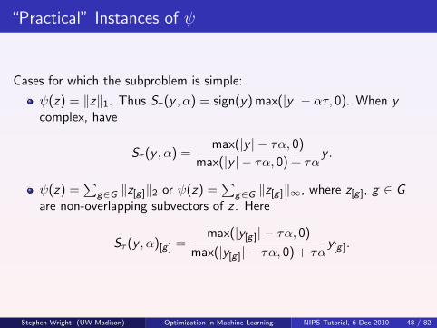
“Practical” Instances of ψ

Cases for which the subproblem is simple:

ψ(z) = ‖z‖1. Thus Sτ (y , α) = sign(y) max(|y | − ατ, 0). When ycomplex, have

Sτ (y , α) =max(|y | − τα, 0)

max(|y | − τα, 0) + ταy .

ψ(z) =∑

g∈G ‖z[g ]‖2 or ψ(z) =∑

g∈G ‖z[g ]‖∞, where z[g ], g ∈ Gare non-overlapping subvectors of z . Here

Sτ (y , α)[g ] =max(|y[g ]| − τα, 0)

max(|y[g ]| − τα, 0) + ταy[g ].


Z is a matrix and ψ(Z ) = ‖Z‖∗ is the nuclear norm of Z : the sum ofsingular values. Threshold operator is

Sτ (Y , α) := arg minZ

1

2α‖Z − Y ‖2

F + τ‖Z‖∗

with solution obtained from the SVD Y = UΣV T with U, Vorthonormal and Σ = diag(σi )i=1,2,...,m. SettingΣ = diag(max(σi − τα, 0)i=1,2,...,m), the solution is

Sτ (Y , α) = UΣV T .

(Actually not cheap to compute, but in some cases (e.g. σi − τα < 0for most i) approximate solutions can be found in reasoable time.)


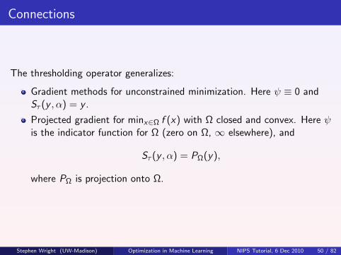
Connections

The thresholding operator generalizes:

Gradient methods for unconstrained minimization. Here ψ ≡ 0 andSτ (y , α) = y .

Projected gradient for minx∈Ω f (x) with Ω closed and convex. Here ψis the indicator function for Ω (zero on Ω, ∞ elsewhere), and

Sτ (y , α) = PΩ(y),

where PΩ is projection onto Ω.


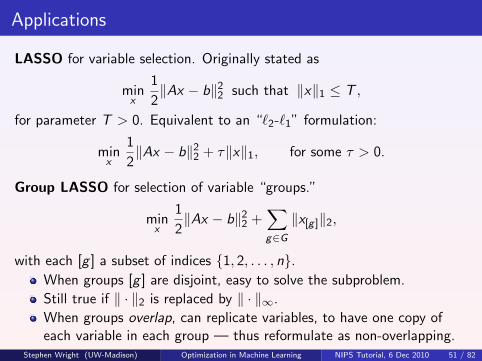
Applications

LASSO for variable selection. Originally stated as

minx

1

2‖Ax − b‖2

2 such that ‖x‖1 ≤ T ,

for parameter T > 0. Equivalent to an “`2-`1” formulation:

minx

1

2‖Ax − b‖2

2 + τ‖x‖1, for some τ > 0.

Group LASSO for selection of variable “groups.”

minx

1

2‖Ax − b‖2

2 +∑g∈G‖x[g ]‖2,

with each [g ] a subset of indices 1, 2, . . . , n.When groups [g ] are disjoint, easy to solve the subproblem.

Still true if ‖ · ‖2 is replaced by ‖ · ‖∞.

When groups overlap, can replicate variables, to have one copy ofeach variable in each group — thus reformulate as non-overlapping.


Compressed Sensing. Sparse signal recovery from noisy measurements.Given matrix A (with more columns than rows) and observation vector y ,seek a sparse x (i.e. few nonzeros) such that Ax ≈ y . Solve

minx

1

2‖Ax − b‖2

2 + τ‖x‖1.

Under “restricted isometry” properties on A (“tall, thin” columnsubmatrices are nearly orthonormal), ‖x‖1 is a good surrogate forcard(x).

Assume that A is not stored explicitly, but matrix-vectormultiplications are available. Hence can compute f and ∇f .

Often need solution for a range of τ values.


`1-Regularized Logistic Regression. Feature vectors xi , i = 1, 2, . . . ,mwith labels ±1. Seek odds function parametrized by w ∈ Rn:

p+(x ; w) := (1 + ewT x)−1, p−(x ; w) := 1− p+(x ; w).

Scaled, negative log likelihood function L(w) is

L(w) = − 1

m

∑yi=−1

log p−(xi ; w) +∑yi=1

log p+(xi ; w)

= − 1

m

∑yi=−1

wT xi −m∑i=1

log(1 + ewT xi )

.To get a sparse w (i.e. classify on the basis of a few features) solve:

minwL(w) + λ‖w‖1.


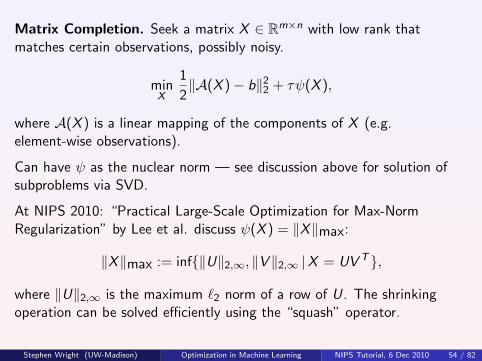
Matrix Completion. Seek a matrix X ∈ Rm×n with low rank thatmatches certain observations, possibly noisy.

minX

1

2‖A(X )− b‖2

2 + τψ(X ),

where A(X ) is a linear mapping of the components of X (e.g.element-wise observations).

Can have ψ as the nuclear norm — see discussion above for solution ofsubproblems via SVD.

At NIPS 2010: “Practical Large-Scale Optimization for Max-NormRegularization” by Lee et al. discuss ψ(X ) = ‖X‖max:

‖X‖max := inf‖U‖2,∞, ‖V ‖2,∞ |X = UV T,

where ‖U‖2,∞ is the maximum `2 norm of a row of U. The shrinkingoperation can be solved efficiently using the “squash” operator.


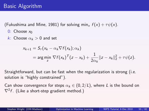
Basic Algorithm

(Fukushima and Mine, 1981) for solving minx f (x) + τψ(x).

0: Choose x0

k : Choose αk > 0 and set

xk+1 = Sτ (xk − αk∇f (xk);αk)

= arg minz∇f (xk)T (z − xk) +

1

2αk‖z − xk‖2

2 + τψ(z).

Straightforward, but can be fast when the regularization is strong (i.e.solution is “highly constrained”).

Can show convergence for steps αk ∈ (0, 2/L), where L is the bound on∇2f . (Like a short-step gradient method.)


Enhancements

Alternatively, since αk plays the role of a steplength, can adjust it to getbetter performance and guaranteed convergence.

“Backtracking:” decrease αk until sufficient decrease condition holds.

Use Barzilai-Borwein strategies to get nonmonotonic methods. Byenforcing sufficient decrease every 10 iterations (say), still get globalconvergence.

The approach can be accelerated using optimal gradient techniques. Seeearlier discussion of FISTA, where we solve the shrinking problem withαk = 1/L in place of a step along −∇f with this steplength.

Note that these methods reduce ultimately to gradient methods on areduced space: the optimal manifold defined by the regularizer ψ.Acceleration or higher-order information can help improve performance.


Continuation in τ

Performance of basic shrinking methods is quite sensitive to τ .

Typically higher τ ⇒ stronger regularization ⇒ optimal manifold has lowerdimension. Hence, it’s easier to identify the optimal manifold, and basicshrinking methods can sometimes do so quickly.

For smaller τ , a simple “continuation” strategy can help:

0: Given target value τf , choose initial τ0 > τf , starting point x andfactor σ ∈ (0, 1).

k: Find approx solution x(τk) of minx f (x) + τψ(x), starting from x ;if τk = τf then STOP;Set τk+1 ← max(τf , στk) and x ← x(τk);


Solution x(τ) is often desired on a range of τ values anyway, soefforts for larger τ are not wasted.

Accelerated methods such as FISTA are less sensitive to the “small τ”issue.

Not much analysis of this approach has been done. Better heuristicsand theoretical support are needed.


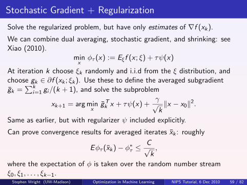
Stochastic Gradient + Regularization

Solve the regularized problem, but have only estimates of ∇f (xk).

We can combine dual averaging, stochastic gradient, and shrinking: seeXiao (2010).

minx

φτ (x) := Eξf (x ; ξ) + τψ(x)

At iteration k choose ξk randomly and i.i.d from the ξ distribution, andchoose gk ∈ ∂f (xk ; ξk). Use these to define the averaged subgradientgk =

∑ki=1 gi/(k + 1), and solve the subproblem

xk+1 = arg minx

gTk x + τψ(x) +

γ√k‖x − x0‖2.

Same as earlier, but with regularizer ψ included explicitly.

Can prove convergence results for averaged iterates xk : roughly

Eφτ (xk)− φ∗τ ≤C√

k,

where the expectation of φ is taken over the random number streamξ0, ξ1, . . . , ξk−1.


Further Reading

1 F. Bach. “Sparse methods for machine learning: Theory and algorithms” Tutorialat NIPS 2009. (Slides on web.)

2 M. Fukushima and H. Mine. “A generalized proximal point algorithm for certainnon-convex minimization problems.” International Journal of Systems Science, 12,pp. 989–1000, 1981.

3 P. L. Combettes and V. R. Wajs. “Signal recovery by proximal forward-backwardsplitting.” Multiscale Modeling and Simulation, 4, pp. 1168–1200, 2005.

4 S. J. Wright, R. D. Nowak, and M. A. T. Figueiredo. “Sparse reconstruction byseparable approximation.” IEEE Transactions on Signal Processing, 57, pp.2479–2493, 2009.

5 E. Candes, J. Romberg, and T. Tao. “Stable signal recovery for incomplete andinaccurate measurements.” Communications in Pure and Applied Mathematics,59, pp. 1207–1223, 2006.

6 L. Xiao. “Dual averaging methods for regularized stochastic learning and onlineoptimization.” TechReport MSR-TR-2010-23, Microsoft Research, March 2010.


IV. Optimal Manifold Identification

When constraints x ∈ Ψ or a nonsmooth regularizer ψ(x) are present,identification of the manifold on which x∗ lies can improve algorithmperformance, by focusing attention on a reduced space. We can thusevaluate partial gradients and Hessians, restricted to just this space.

For nonsmooth regularizer ψ, the active manifold is a smooth surfacepassing through x∗ along which ψ is smooth.Example: for ψ(x) = ‖x‖1, have manifold consisting of z with

zi

≥ 0 if x∗i > 0

≤ 0 if x∗i < 0

= 0 if x∗i = 0.


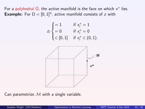
For a polyhedral Ω, the active manifold is the face on which x∗ lies.Example: For Ω = [0, 1]n, active manifold consists of z with

zi

= 1 if x∗i = 1

= 0 if x∗i = 0

∈ [0, 1] if x∗i ∈ (0, 1).

M

x*

Can parametrize M with a single variable.


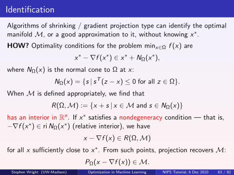
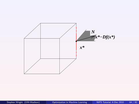
Identification

Algorithms of shrinking / gradient projection type can identify the optimalmanifold M, or a good approximation to it, without knowing x∗.

HOW? Optimality conditions for the problem minx∈Ω f (x) are

x∗ −∇f (x∗) ∈ x∗ + NΩ(x∗),

where NΩ(x) is the normal cone to Ω at x :

NΩ(x) = s | sT (z − x) ≤ 0 for all z ∈ Ω.When M is defined appropriately, we find that

R(Ω,M) := x + s | x ∈M and s ∈ NΩ(x)has an interior in Rn. If x∗ satisfies a nondegeneracy condition — that is,−∇f (x∗) ∈ ri NΩ(x∗) (relative interior), we have

x −∇f (x) ∈ R(Ω,M)

for all x sufficiently close to x∗. From such points, projection recovers M:

PΩ(x −∇f (x)) ∈M.


x*−Df(x*)

x*

N


The non-averaged iterates from gradient projection methods eventually lieon the correct manifold M. The same is true for dual-averaging methods(where the gradient term is averaged over all steps).

When we have a nonsmooth regularizer ψ, instead of Ω, the analogousproperty is that the solution of the shrink subproblem, for some fixedpositive α, lies on the optimal manifold M.

Under reasonable conditions on αk , the “basic” shrink method eventuallyhas all its iterates on M. Also true for dual-averaged methods.

In practice, often use heuristics for deciding when M (or a small superset)has been reached. If a distance-to-solution bound is available, and ifLipschitz constant for ∇f is known, can make this decision more rigorous.


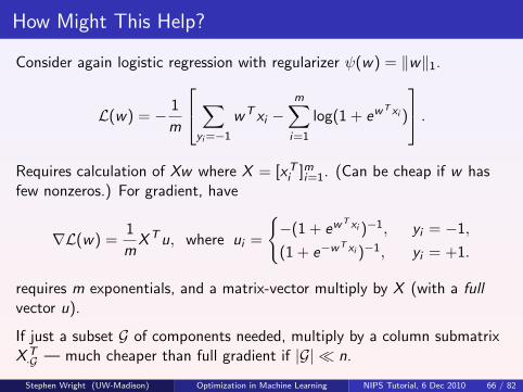
How Might This Help?

Consider again logistic regression with regularizer ψ(w) = ‖w‖1.

L(w) = − 1

m

∑yi=−1

wT xi −m∑i=1

log(1 + ewT xi )

.Requires calculation of Xw where X = [xT

i ]mi=1. (Can be cheap if w hasfew nonzeros.) For gradient, have

∇L(w) =1

mXTu, where ui =

−(1 + ew

T xi )−1, yi = −1,

(1 + e−wT xi )−1, yi = +1.

requires m exponentials, and a matrix-vector multiply by X (with a fullvector u).

If just a subset G of components needed, multiply by a column submatrixXT·G — much cheaper than full gradient if |G| n.


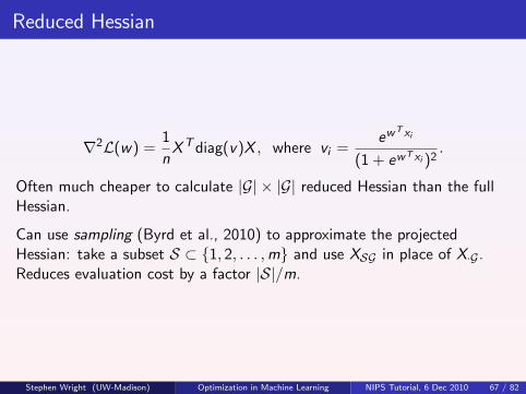
Reduced Hessian

∇2L(w) =1

nXTdiag(v)X , where vi =

ewT xi

(1 + ewT xi )2.

Often much cheaper to calculate |G| × |G| reduced Hessian than the fullHessian.

Can use sampling (Byrd et al., 2010) to approximate the projectedHessian: take a subset S ⊂ 1, 2, . . . ,m and use XSG in place of X·G .Reduces evaluation cost by a factor |S|/m.


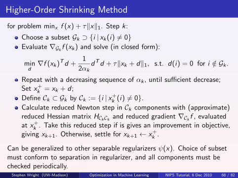
Higher-Order Shrinking Method

for problem minx f (x) + τ‖x‖1. Step k :

Choose a subset Gk ⊃ i | xk(i) 6= 0Evaluate ∇Gk f (xk) and solve (in closed form):

mind∇f (xk)Td +

1

2αkdTd + τ‖xk + d‖1, s.t. d(i) = 0 for i /∈ Gk .

Repeat with a decreasing sequence of αk , until sufficient decrease;Set x+

k = xk + d ;

Define Ck ⊂ Gk by Ck := i | x+k (i) 6= 0.

Calculate reduced Newton step in Ck components with (approximate)reduced Hessian matrix HCkCk and reduced gradient ∇Ck f , evaluatedat x+

k . Take this reduced step if is gives an improvement in objective,giving xk+1. Otherwise, settle for xk+1 ← x+

k .

Can be generalized to other separable regularizers ψ(x). Choice of subsetmust conform to separation in regularizer, and all components must bechecked periodically.


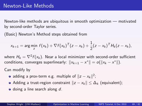
Newton-Like Methods

Newton-like methods are ubiquitous in smooth optimization — motivatedby second-order Taylor series.

(Basic) Newton’s Method steps obtained from

xk+1 = arg minz

f (xk) +∇f (xk)T (z − xk) +1

2(z − xk)THk(z − xk),

where Hk = ∇2f (xk). Near a local minimizer with second-order sufficientconditions, converges superlinearly: ‖xk+1 − x∗‖ = o(‖xk − x∗‖).

Can modify by

adding a prox-term e.g. multiple of ‖z − xk‖2;

Adding a trust-region constraint ‖z − xk‖ ≤ ∆k (equivalent);

doing a line search along d .


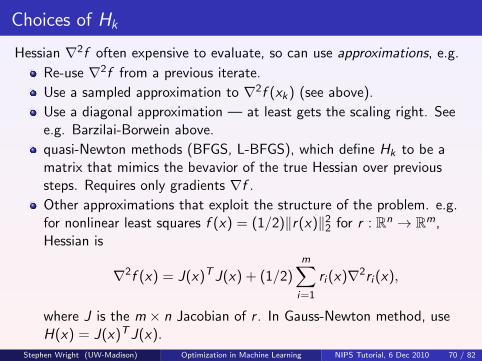
Choices of Hk

Hessian ∇2f often expensive to evaluate, so can use approximations, e.g.

Re-use ∇2f from a previous iterate.

Use a sampled approximation to ∇2f (xk) (see above).

Use a diagonal approximation — at least gets the scaling right. Seee.g. Barzilai-Borwein above.

quasi-Newton methods (BFGS, L-BFGS), which define Hk to be amatrix that mimics the bevavior of the true Hessian over previoussteps. Requires only gradients ∇f .

Other approximations that exploit the structure of the problem. e.g.for nonlinear least squares f (x) = (1/2)‖r(x)‖2

2 for r : Rn → Rm,Hessian is

∇2f (x) = J(x)T J(x) + (1/2)m∑i=1

ri (x)∇2ri (x),

where J is the m × n Jacobian of r . In Gauss-Newton method, useH(x) = J(x)T J(x).


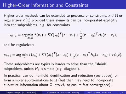
Higher-Order Information and Constraints

Higher-order methods can be extended to presence of constraints x ∈ Ω orregularizers ψ(x) provided these elements can be incorporated explicitlyinto the subproblems. e.g. for constraints

xk+1 = arg minz∈Ω

f (xk) +∇f (xk)T (z − xk) +1

2(z − xk)THk(z − xk),

and for regularizers

xk+1 = arg minz

f (xk) +∇f (xk)T (z − xk) +1

2(z − xk)THk(z − xk) + τψ(z).

These subproblems are typically harder to solve than the “shrink”subproblem, unless Hk is simple (e.g. diagonal).

In practice, can do manifold identification and reduction (see above), orform simpler approximations to Ω (but then may need to incorporatecurvature information about Ω into Hk to ensure fast convergence).


Solving for xk+1

When Hk positive definite, can solve Newton equations explicitly by solving

Hk(z − xk) = −∇f (xk).

Alternatively, apply conjugate gradient to this system to get an inexactsolution. Each iterate requires a multiplication by Hk .

Can precondition CG, e.g. by using sample approximations, structuredapproximations, or Krylov subspace information gathered at previousevaluations of ∇2f .

L-BFGS stores Hk in implicit form, by means of 2m vectors in Rn, for asmall parameter m (e.g. 5). Recovers solution of the equation above via2m inner products.


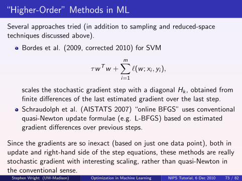
“Higher-Order” Methods in ML

Several approaches tried (in addition to sampling and reduced-spacetechniques discussed above).

Bordes et al. (2009, corrected 2010) for SVM

τwTw +m∑i=1

`(w ; xi , yi ),

scales the stochastic gradient step with a diagonal Hk , obtained fromfinite differences of the last estimated gradient over the last step.

Schraudolph et al. (AISTATS 2007) “online BFGS” uses conventionalquasi-Newton update formulae (e.g. L-BFGS) based on estimatedgradient differences over previous steps.

Since the gradients are so inexact (based on just one data point), both inupdate and right-hand side of the step equations, these methods are reallystochastic gradient with interesting scaling, rather than quasi-Newton inthe conventional sense.


Further Reading

1 L. Bottou and A. Moore, “Learning with large datasets,” Tutorial at NIPS 2007(slides on web).

2 J. Nocedal and S. J. Wright, Numerical Optimization, 2nd edition, Springer, 2006.

3 R. H. Byrd, G. M. Chin, W. Neveitt, and J. Nocedal. “On the use of stochastichessian information in unconstrained optimization.” Technical Report,Northwestern University, June 2010.

4 M. Fisher, J. Nocedal, Y. Tremolet, and S. J. Wright. “Data assimilation inweather forecasting: A case study in PDE-constrained optimization.” Optimizationand Engineering, 10, pp. 409–426, 2009.

5 A. S. Lewis and S. J. Wright. “Identifying activity.” Technical report, ORIE,Cornell University. Revised April 2010.

6 S. J. Wright, “Accelerated block-coordinate relaxation for regularizedoptimization,” Technical Report, August 2010.

7 W. Hare and A. Lewis. “Identifying active constraints via partial smoothness andprox-regularity.” Journal of Convex Analysis, 11, pp. 251–266, 2004.


V. Decomposition / Coordinate Relaxation

For min f (x), at iteration k, choose a subset Gk ⊂ 1, 2, . . . , n and takea step dk only in these components. i.e. fix dk(i) = 0 for i /∈ Gk .

Gives more manageable subproblem sizes, in practice.

Can

take a reduced gradient step in the Gk components;

take multiple “inner iterations”

actually solve the reduced subproblem in the space defined by Gk .


Constraints and Regularizers Complicate Things

For minx∈Ω f (x), need to put enough components into Gk to stay feasible,as well as make progress.

Example: min f (x1, x2) with x1 + x2 = 1. Relaxation with Gk = 1 orGk = 2 won’t work.

For separable regularizer (e.g. Group LASSO) with

ψ(x) =∑g∈G

ψg (x[g ]),

need to ensure that Gk is a union of the some index subsets [g ]. i.e. therelaxation components must be consonant with the partitioning.


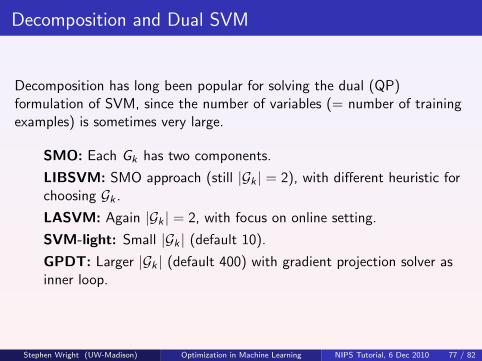
Decomposition and Dual SVM

Decomposition has long been popular for solving the dual (QP)formulation of SVM, since the number of variables (= number of trainingexamples) is sometimes very large.

SMO: Each Gk has two components.

LIBSVM: SMO approach (still |Gk | = 2), with different heuristic forchoosing Gk .

LASVM: Again |Gk | = 2, with focus on online setting.

SVM-light: Small |Gk | (default 10).

GPDT: Larger |Gk | (default 400) with gradient projection solver asinner loop.


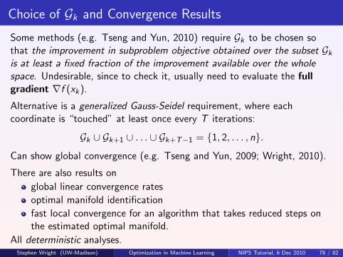
Choice of Gk and Convergence Results

Some methods (e.g. Tseng and Yun, 2010) require Gk to be chosen sothat the improvement in subproblem objective obtained over the subset Gkis at least a fixed fraction of the improvement available over the wholespace. Undesirable, since to check it, usually need to evaluate the fullgradient ∇f (xk).

Alternative is a generalized Gauss-Seidel requirement, where eachcoordinate is “touched” at least once every T iterations:

Gk ∪ Gk+1 ∪ . . . ∪ Gk+T−1 = 1, 2, . . . , n.

Can show global convergence (e.g. Tseng and Yun, 2009; Wright, 2010).

There are also results on

global linear convergence rates

optimal manifold identification

fast local convergence for an algorithm that takes reduced steps onthe estimated optimal manifold.

All deterministic analyses.Stephen Wright (UW-Madison) Optimization in Machine Learning NIPS Tutorial, 6 Dec 2010 78 / 82

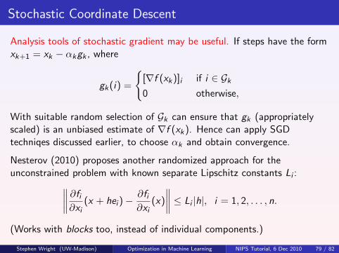
Stochastic Coordinate Descent

Analysis tools of stochastic gradient may be useful. If steps have the formxk+1 = xk − αkgk , where

gk(i) =

[∇f (xk)]i if i ∈ Gk0 otherwise,

With suitable random selection of Gk can ensure that gk (appropriatelyscaled) is an unbiased estimate of ∇f (xk). Hence can apply SGDtechniqes discussed earlier, to choose αk and obtain convergence.

Nesterov (2010) proposes another randomized approach for theunconstrained problem with known separate Lipschitz constants Li :∥∥∥∥ ∂fi

∂xi(x + hei )−

∂fi∂xi

(x)

∥∥∥∥ ≤ Li |h|, i = 1, 2, . . . , n.

(Works with blocks too, instead of individual components.)


At step k :

Choose index ik ∈ 1, 2, . . . , n with probability pi := Li/(∑n

j=1 Lj);

Take gradient step in ik component:

xk+1 = xk −1

Lik

∂f

∂xikeik .

Basic convergence result:

E [f (xk)]− f ∗ ≤ C

k.

As for SA (earlier) but without any strong convexity assumption.

Can also get linear convergence results (in expectation) by assumingstrong convexity in f , according to different norms.

Can also accelerate in the usual fashion (see above), to improve expectedconvergence rate to O(1/k2).


Further Reading

1 P. Tseng and S. Yun, “A coordinate gradient descent method for linearlyconstrained smooth optimization and support vector machines training.”Computational Optimization and Applications, 47, pp. 179–206, 2010.

2 P. Tseng and S. Yun, “A coordinate gradient descent method for nonsmoothseparable minimization.” Mathematical Programming, Series B, 117. pp.387–423, 2009.

3 S. J. Wright, “Accelerated block-coordinate relaxation for regularizedoptimization.” Technical Report, UW-Madison, August 2010.

4 Y. Nesterov, “Efficiency of coordinate descent methods on huge-scale optimizationproblems.” CORE Discussion Paper 2010/2, CORE, UCL, January 2010.


Conclusions

We’ve surveyed a number of topics in algorithmic fundamentals, with aneye on recent developments, and on topics of relevance (current or future)to machine learning.

The talk was far from exhaustive. Literature on Optimization in ML ishuge and growing.

There is much more to be gained from the interaction between the twoareas.

FIN


nips2010: optimization algorithms in machine learning

Education

f xk f x

xk f xk

f x0 f x

nonsmooth f f

obtaink f xk

f x li

objective f

x0 x2 f xk