neural network toolbox™ user’s guide...environment and neural network toolbox software. example...
TRANSCRIPT

Neural Network Toolbox™
User’s Guide
R2012b
Mark Hudson BealeMartin T. HaganHoward B. Demuth

How to Contact MathWorks
www.mathworks.com Webcomp.soft-sys.matlab Newsgroupwww.mathworks.com/contact_TS.html Technical Support
[email protected] Product enhancement [email protected] Bug [email protected] Documentation error [email protected] Order status, license renewals, [email protected] Sales, pricing, and general information
508-647-7000 (Phone)
508-647-7001 (Fax)
The MathWorks, Inc.3 Apple Hill DriveNatick, MA 01760-2098For contact information about worldwide offices, see the MathWorks Web site.
Neural Network Toolbox™ User’s Guide
© COPYRIGHT 1992–2012 by The MathWorks, Inc.The software described in this document is furnished under a license agreement. The software may be usedor copied only under the terms of the license agreement. No part of this manual may be photocopied orreproduced in any form without prior written consent from The MathWorks, Inc.
FEDERAL ACQUISITION: This provision applies to all acquisitions of the Program and Documentationby, for, or through the federal government of the United States. By accepting delivery of the Programor Documentation, the government hereby agrees that this software or documentation qualifies ascommercial computer software or commercial computer software documentation as such terms are usedor defined in FAR 12.212, DFARS Part 227.72, and DFARS 252.227-7014. Accordingly, the terms andconditions of this Agreement and only those rights specified in this Agreement, shall pertain to and governthe use, modification, reproduction, release, performance, display, and disclosure of the Program andDocumentation by the federal government (or other entity acquiring for or through the federal government)and shall supersede any conflicting contractual terms or conditions. If this License fails to meet thegovernment’s needs or is inconsistent in any respect with federal procurement law, the government agreesto return the Program and Documentation, unused, to The MathWorks, Inc.
Trademarks
MATLAB and Simulink are registered trademarks of The MathWorks, Inc. Seewww.mathworks.com/trademarks for a list of additional trademarks. Other product or brandnames may be trademarks or registered trademarks of their respective holders.
Patents
MathWorks products are protected by one or more U.S. patents. Please seewww.mathworks.com/patents for more information.

Revision HistoryJune 1992 First printingApril 1993 Second printingJanuary 1997 Third printingJuly 1997 Fourth printingJanuary 1998 Fifth printing Revised for Version 3 (Release 11)September 2000 Sixth printing Revised for Version 4 (Release 12)June 2001 Seventh printing Minor revisions (Release 12.1)July 2002 Online only Minor revisions (Release 13)January 2003 Online only Minor revisions (Release 13SP1)June 2004 Online only Revised for Version 4.0.3 (Release 14)October 2004 Online only Revised for Version 4.0.4 (Release 14SP1)October 2004 Eighth printing Revised for Version 4.0.4March 2005 Online only Revised for Version 4.0.5 (Release 14SP2)March 2006 Online only Revised for Version 5.0 (Release 2006a)September 2006 Ninth printing Minor revisions (Release 2006b)March 2007 Online only Minor revisions (Release 2007a)September 2007 Online only Revised for Version 5.1 (Release 2007b)March 2008 Online only Revised for Version 6.0 (Release 2008a)October 2008 Online only Revised for Version 6.0.1 (Release 2008b)March 2009 Online only Revised for Version 6.0.2 (Release 2009a)September 2009 Online only Revised for Version 6.0.3 (Release 2009b)March 2010 Online only Revised for Version 6.0.4 (Release 2010a)September 2010 Online only Revised for Version 7.0 (Release 2010b)April 2011 Online only Revised for Version 7.0.1 (Release 2011a)September 2011 Online only Revised for Version 7.0.2 (Release 2011b)March 2012 Online only Revised for Version 7.0.3 (Release 2012a)September 2012 Online only Revised for Version 8.0 (Release 2012b)


Contents
Neural Network Toolbox Design Book
Network Objects, Data, and Training Styles
1Introduction . . . . . . . . . . . . . . . . . . . . . . . . . . . . . . . . . . . . . . 1-2
Neuron Model . . . . . . . . . . . . . . . . . . . . . . . . . . . . . . . . . . . . . 1-4Simple Neuron . . . . . . . . . . . . . . . . . . . . . . . . . . . . . . . . . . . . 1-4Transfer Functions . . . . . . . . . . . . . . . . . . . . . . . . . . . . . . . . 1-5Neuron with Vector Input . . . . . . . . . . . . . . . . . . . . . . . . . . . 1-6
Network Architectures . . . . . . . . . . . . . . . . . . . . . . . . . . . . . 1-10One Layer of Neurons . . . . . . . . . . . . . . . . . . . . . . . . . . . . . . 1-10Multiple Layers of Neurons . . . . . . . . . . . . . . . . . . . . . . . . . 1-12Input and Output Processing Functions . . . . . . . . . . . . . . . 1-14
Network Object . . . . . . . . . . . . . . . . . . . . . . . . . . . . . . . . . . . . 1-16
Configuration . . . . . . . . . . . . . . . . . . . . . . . . . . . . . . . . . . . . . 1-21
Data Structures . . . . . . . . . . . . . . . . . . . . . . . . . . . . . . . . . . . 1-24Simulation with Concurrent Inputs in a Static Network . . 1-24Simulation with Sequential Inputs in a DynamicNetwork . . . . . . . . . . . . . . . . . . . . . . . . . . . . . . . . . . . . . . . 1-25
Simulation with Concurrent Inputs in a DynamicNetwork . . . . . . . . . . . . . . . . . . . . . . . . . . . . . . . . . . . . . . . 1-27
Training Styles (Adapt and Train) . . . . . . . . . . . . . . . . . . . 1-30Incremental Training with adapt . . . . . . . . . . . . . . . . . . . . . 1-30Batch Training . . . . . . . . . . . . . . . . . . . . . . . . . . . . . . . . . . . 1-33Training Feedback . . . . . . . . . . . . . . . . . . . . . . . . . . . . . . . . 1-36
v
Multilayer Networks and BackpropagationTraining
2Multilayer Networks and Backpropagation Training . . 2-2
Multilayer Neural Network Architecture . . . . . . . . . . . . 2-3Neuron Model (logsig, tansig, purelin) . . . . . . . . . . . . . . . . . 2-3Feedforward Network . . . . . . . . . . . . . . . . . . . . . . . . . . . . . . 2-4
Collect and Prepare the Data . . . . . . . . . . . . . . . . . . . . . . . 2-7Preprocessing and Postprocessing . . . . . . . . . . . . . . . . . . . . 2-7Dividing the Data . . . . . . . . . . . . . . . . . . . . . . . . . . . . . . . . . 2-10
Create, Configure, and Initialize the Network . . . . . . . . 2-13Other Related Architectures . . . . . . . . . . . . . . . . . . . . . . . . . 2-14Initializing Weights (init) . . . . . . . . . . . . . . . . . . . . . . . . . . . 2-14
Train the Network . . . . . . . . . . . . . . . . . . . . . . . . . . . . . . . . . 2-15Training Algorithms . . . . . . . . . . . . . . . . . . . . . . . . . . . . . . . 2-16Efficiency and Memory Reduction . . . . . . . . . . . . . . . . . . . . 2-18Generalization . . . . . . . . . . . . . . . . . . . . . . . . . . . . . . . . . . . . 2-18Training Example . . . . . . . . . . . . . . . . . . . . . . . . . . . . . . . . . 2-19
Post-Training Analysis (Network Validation) . . . . . . . . . 2-23Improving Results . . . . . . . . . . . . . . . . . . . . . . . . . . . . . . . . . 2-26
Use the Network . . . . . . . . . . . . . . . . . . . . . . . . . . . . . . . . . . . 2-28
Automatic Code Generation . . . . . . . . . . . . . . . . . . . . . . . . 2-29
Limitations and Cautions . . . . . . . . . . . . . . . . . . . . . . . . . . 2-30
vi Contents
Dynamic Networks
3Introduction . . . . . . . . . . . . . . . . . . . . . . . . . . . . . . . . . . . . . . 3-2Examples of Dynamic Networks . . . . . . . . . . . . . . . . . . . . . 3-3Applications of Dynamic Networks . . . . . . . . . . . . . . . . . . . 3-9Dynamic Network Structures . . . . . . . . . . . . . . . . . . . . . . . . 3-9Dynamic Network Training . . . . . . . . . . . . . . . . . . . . . . . . . 3-11
Focused Time-Delay Neural Network (timedelaynet) . . 3-13
Preparing Data (preparets) . . . . . . . . . . . . . . . . . . . . . . . . . 3-18
Distributed Time-Delay Neural Network(distdelaynet) . . . . . . . . . . . . . . . . . . . . . . . . . . . . . . . . . . . 3-20
NARX Network (narxnet, closeloop) . . . . . . . . . . . . . . . . . 3-23
Layer-Recurrent Network (layrecnet) . . . . . . . . . . . . . . . 3-29
Training Custom Networks . . . . . . . . . . . . . . . . . . . . . . . . . 3-31
Multiple Sequences, Time-Series Utilities, and ErrorWeighting . . . . . . . . . . . . . . . . . . . . . . . . . . . . . . . . . . . . . . . 3-37Multiple Sequences . . . . . . . . . . . . . . . . . . . . . . . . . . . . . . . . 3-37Time-Series Utilities . . . . . . . . . . . . . . . . . . . . . . . . . . . . . . . 3-38Error Weighting . . . . . . . . . . . . . . . . . . . . . . . . . . . . . . . . . . 3-40
Control Systems
4Introduction to System Control . . . . . . . . . . . . . . . . . . . . . 4-2
NN Predictive Control . . . . . . . . . . . . . . . . . . . . . . . . . . . . . 4-4System Identification . . . . . . . . . . . . . . . . . . . . . . . . . . . . . . 4-4Predictive Control . . . . . . . . . . . . . . . . . . . . . . . . . . . . . . . . . 4-5
vii
Use the NN Predictive Controller Block . . . . . . . . . . . . . . . 4-6
NARMA-L2 (Feedback Linearization) Control . . . . . . . . 4-14Identification of the NARMA-L2 Model . . . . . . . . . . . . . . . . 4-14NARMA-L2 Controller . . . . . . . . . . . . . . . . . . . . . . . . . . . . . 4-16Use the NARMA-L2 Controller Block . . . . . . . . . . . . . . . . . 4-18
Model Reference Control . . . . . . . . . . . . . . . . . . . . . . . . . . . 4-23Use the Model Reference Controller Block . . . . . . . . . . . . . 4-24
Import and Export . . . . . . . . . . . . . . . . . . . . . . . . . . . . . . . . . 4-31Import and Export Networks . . . . . . . . . . . . . . . . . . . . . . . . 4-31Import and Export Training Data . . . . . . . . . . . . . . . . . . . . 4-35
Radial Basis Networks
5Introduction . . . . . . . . . . . . . . . . . . . . . . . . . . . . . . . . . . . . . . 5-2Important Radial Basis Functions . . . . . . . . . . . . . . . . . . . . 5-2
Radial Basis Functions . . . . . . . . . . . . . . . . . . . . . . . . . . . . . 5-3Neuron Model . . . . . . . . . . . . . . . . . . . . . . . . . . . . . . . . . . . . 5-3Network Architecture . . . . . . . . . . . . . . . . . . . . . . . . . . . . . . 5-4Exact Design (newrbe) . . . . . . . . . . . . . . . . . . . . . . . . . . . . . 5-5More Efficient Design (newrb) . . . . . . . . . . . . . . . . . . . . . . . 5-7Examples . . . . . . . . . . . . . . . . . . . . . . . . . . . . . . . . . . . . . . . . 5-8
Probabilistic Neural Networks . . . . . . . . . . . . . . . . . . . . . . 5-10Network Architecture . . . . . . . . . . . . . . . . . . . . . . . . . . . . . . 5-10Design (newpnn) . . . . . . . . . . . . . . . . . . . . . . . . . . . . . . . . . . 5-11
Generalized Regression Networks . . . . . . . . . . . . . . . . . . . 5-13Network Architecture . . . . . . . . . . . . . . . . . . . . . . . . . . . . . . 5-13Design (newgrnn) . . . . . . . . . . . . . . . . . . . . . . . . . . . . . . . . . 5-15
viii Contents

Self-Organizing and Learning VectorQuantization Nets
6Introduction . . . . . . . . . . . . . . . . . . . . . . . . . . . . . . . . . . . . . . 6-2Important Self-Organizing and LVQ Functions . . . . . . . . . 6-2
Competitive Learning . . . . . . . . . . . . . . . . . . . . . . . . . . . . . . 6-3Architecture . . . . . . . . . . . . . . . . . . . . . . . . . . . . . . . . . . . . . . 6-3Creating a Competitive Neural Network (competlayer) . . . 6-4Kohonen Learning Rule (learnk) . . . . . . . . . . . . . . . . . . . . . 6-5Bias Learning Rule (learncon) . . . . . . . . . . . . . . . . . . . . . . . 6-5Training . . . . . . . . . . . . . . . . . . . . . . . . . . . . . . . . . . . . . . . . . 6-6Graphical Example . . . . . . . . . . . . . . . . . . . . . . . . . . . . . . . . 6-8
Self-Organizing Feature Maps . . . . . . . . . . . . . . . . . . . . . . 6-10Topologies (gridtop, hextop, randtop) . . . . . . . . . . . . . . . . . . 6-11Distance Functions (dist, linkdist, mandist, boxdist) . . . . . 6-15Architecture . . . . . . . . . . . . . . . . . . . . . . . . . . . . . . . . . . . . . . 6-18Create a Self-Organizing Map Neural Network(selforgmap) . . . . . . . . . . . . . . . . . . . . . . . . . . . . . . . . . . . . 6-19
Training (learnsomb) . . . . . . . . . . . . . . . . . . . . . . . . . . . . . . 6-22Examples . . . . . . . . . . . . . . . . . . . . . . . . . . . . . . . . . . . . . . . . 6-25
Learning Vector Quantization Networks . . . . . . . . . . . . . 6-37Architecture . . . . . . . . . . . . . . . . . . . . . . . . . . . . . . . . . . . . . . 6-37Creating an LVQ Network . . . . . . . . . . . . . . . . . . . . . . . . . . 6-38LVQ1 Learning Rule (learnlv1) . . . . . . . . . . . . . . . . . . . . . . 6-41Training . . . . . . . . . . . . . . . . . . . . . . . . . . . . . . . . . . . . . . . . . 6-43Supplemental LVQ2.1 Learning Rule (learnlv2) . . . . . . . . . 6-45
Adaptive Filters and Adaptive Training
7Introduction . . . . . . . . . . . . . . . . . . . . . . . . . . . . . . . . . . . . . . 7-2Important Adaptive Functions . . . . . . . . . . . . . . . . . . . . . . . 7-2
ix
Linear Neuron Model . . . . . . . . . . . . . . . . . . . . . . . . . . . . . . 7-3
Adaptive Linear Network Architecture . . . . . . . . . . . . . . 7-4Single ADALINE (linearlayer) . . . . . . . . . . . . . . . . . . . . . . . 7-4
Least Mean Square Error . . . . . . . . . . . . . . . . . . . . . . . . . . . 7-8
LMS Algorithm (learnwh) . . . . . . . . . . . . . . . . . . . . . . . . . . 7-9
Adaptive Filtering (adapt) . . . . . . . . . . . . . . . . . . . . . . . . . . 7-10Tapped Delay Line . . . . . . . . . . . . . . . . . . . . . . . . . . . . . . . . 7-10Adaptive Filter . . . . . . . . . . . . . . . . . . . . . . . . . . . . . . . . . . . 7-10Adaptive Filter Example . . . . . . . . . . . . . . . . . . . . . . . . . . . . 7-11Prediction Example . . . . . . . . . . . . . . . . . . . . . . . . . . . . . . . . 7-14Noise Cancelation Example . . . . . . . . . . . . . . . . . . . . . . . . . 7-15Multiple Neuron Adaptive Filters . . . . . . . . . . . . . . . . . . . . 7-17
Advanced Topics
8Parallel and GPU Computing . . . . . . . . . . . . . . . . . . . . . . . 8-2Modes of Parallelism . . . . . . . . . . . . . . . . . . . . . . . . . . . . . . . 8-2Distributed Computing . . . . . . . . . . . . . . . . . . . . . . . . . . . . . 8-3Single GPU Computing . . . . . . . . . . . . . . . . . . . . . . . . . . . . . 8-6Distributed GPU Computing . . . . . . . . . . . . . . . . . . . . . . . . 8-9Parallel Time Series . . . . . . . . . . . . . . . . . . . . . . . . . . . . . . . 8-11Parallel Availability, Fallbacks, and Feedback . . . . . . . . . . 8-11
Speed and Memory Optimizations . . . . . . . . . . . . . . . . . . . 8-14Memory Reduction . . . . . . . . . . . . . . . . . . . . . . . . . . . . . . . . 8-14Fast Elliot Sigmoid . . . . . . . . . . . . . . . . . . . . . . . . . . . . . . . . 8-14
Multilayer Training Speed and Memory . . . . . . . . . . . . . 8-17SIN Data Set . . . . . . . . . . . . . . . . . . . . . . . . . . . . . . . . . . . . . 8-18PARITY Data Set . . . . . . . . . . . . . . . . . . . . . . . . . . . . . . . . . 8-20ENGINE Data Set . . . . . . . . . . . . . . . . . . . . . . . . . . . . . . . . . 8-23CANCER Data Set . . . . . . . . . . . . . . . . . . . . . . . . . . . . . . . . 8-25CHOLESTEROL Data Set . . . . . . . . . . . . . . . . . . . . . . . . . . 8-27
x Contents
DIABETES Data Set . . . . . . . . . . . . . . . . . . . . . . . . . . . . . . . 8-30Summary . . . . . . . . . . . . . . . . . . . . . . . . . . . . . . . . . . . . . . . . 8-32
Improving Generalization . . . . . . . . . . . . . . . . . . . . . . . . . . 8-34Early Stopping . . . . . . . . . . . . . . . . . . . . . . . . . . . . . . . . . . . . 8-35Index Data Division (divideind) . . . . . . . . . . . . . . . . . . . . . . 8-36Random Data Division (dividerand) . . . . . . . . . . . . . . . . . . 8-36Block Data Division (divideblock) . . . . . . . . . . . . . . . . . . . . 8-37Interleaved Data Division (divideint) . . . . . . . . . . . . . . . . . 8-37Regularization . . . . . . . . . . . . . . . . . . . . . . . . . . . . . . . . . . . . 8-37Summary and Discussion of Early Stopping andRegularization . . . . . . . . . . . . . . . . . . . . . . . . . . . . . . . . . . 8-41
Posttraining Analysis (postreg) . . . . . . . . . . . . . . . . . . . . . . 8-43
Custom Networks . . . . . . . . . . . . . . . . . . . . . . . . . . . . . . . . . . 8-46Custom Network . . . . . . . . . . . . . . . . . . . . . . . . . . . . . . . . . . 8-46Network Definition . . . . . . . . . . . . . . . . . . . . . . . . . . . . . . . . 8-47Network Behavior . . . . . . . . . . . . . . . . . . . . . . . . . . . . . . . . . 8-57
Additional Toolbox Functions . . . . . . . . . . . . . . . . . . . . . . 8-60
Custom Functions . . . . . . . . . . . . . . . . . . . . . . . . . . . . . . . . . 8-61
Historical Networks
9Introduction . . . . . . . . . . . . . . . . . . . . . . . . . . . . . . . . . . . . . . 9-2
Perceptron Networks . . . . . . . . . . . . . . . . . . . . . . . . . . . . . . 9-3Neuron Model . . . . . . . . . . . . . . . . . . . . . . . . . . . . . . . . . . . . 9-3Perceptron Architecture . . . . . . . . . . . . . . . . . . . . . . . . . . . . 9-5Create a Perceptron . . . . . . . . . . . . . . . . . . . . . . . . . . . . . . . 9-6Perceptron Learning Rule (learnp) . . . . . . . . . . . . . . . . . . . 9-7Training (train) . . . . . . . . . . . . . . . . . . . . . . . . . . . . . . . . . . . 9-10Limitations and Cautions . . . . . . . . . . . . . . . . . . . . . . . . . . . 9-16
Linear Networks . . . . . . . . . . . . . . . . . . . . . . . . . . . . . . . . . . 9-18Neuron Model . . . . . . . . . . . . . . . . . . . . . . . . . . . . . . . . . . . . 9-18
xi
Network Architecture . . . . . . . . . . . . . . . . . . . . . . . . . . . . . . 9-19Least Mean Square Error . . . . . . . . . . . . . . . . . . . . . . . . . . . 9-23Linear System Design (newlind) . . . . . . . . . . . . . . . . . . . . . 9-23Linear Networks with Delays . . . . . . . . . . . . . . . . . . . . . . . . 9-24LMS Algorithm (learnwh) . . . . . . . . . . . . . . . . . . . . . . . . . . . 9-27Linear Classification (train) . . . . . . . . . . . . . . . . . . . . . . . . . 9-29Limitations and Cautions . . . . . . . . . . . . . . . . . . . . . . . . . . . 9-31
Hopfield Network . . . . . . . . . . . . . . . . . . . . . . . . . . . . . . . . . . 9-34Fundamentals . . . . . . . . . . . . . . . . . . . . . . . . . . . . . . . . . . . . 9-34Architecture . . . . . . . . . . . . . . . . . . . . . . . . . . . . . . . . . . . . . . 9-34Design (newhop) . . . . . . . . . . . . . . . . . . . . . . . . . . . . . . . . . . 9-36
Summary . . . . . . . . . . . . . . . . . . . . . . . . . . . . . . . . . . . . . . . . . 9-41Functions . . . . . . . . . . . . . . . . . . . . . . . . . . . . . . . . . . . . . . . . 9-41
Network Object Reference
10Network Properties . . . . . . . . . . . . . . . . . . . . . . . . . . . . . . . . 10-2General . . . . . . . . . . . . . . . . . . . . . . . . . . . . . . . . . . . . . . . . . 10-2Efficiency . . . . . . . . . . . . . . . . . . . . . . . . . . . . . . . . . . . . . . . . 10-2Architecture . . . . . . . . . . . . . . . . . . . . . . . . . . . . . . . . . . . . . . 10-3Subobject Structures . . . . . . . . . . . . . . . . . . . . . . . . . . . . . . . 10-7Functions . . . . . . . . . . . . . . . . . . . . . . . . . . . . . . . . . . . . . . . . 10-9Weight and Bias Values . . . . . . . . . . . . . . . . . . . . . . . . . . . . 10-12
Subobject Properties . . . . . . . . . . . . . . . . . . . . . . . . . . . . . . . 10-15Inputs . . . . . . . . . . . . . . . . . . . . . . . . . . . . . . . . . . . . . . . . . . . 10-15Layers . . . . . . . . . . . . . . . . . . . . . . . . . . . . . . . . . . . . . . . . . . 10-17Outputs . . . . . . . . . . . . . . . . . . . . . . . . . . . . . . . . . . . . . . . . . 10-23Biases . . . . . . . . . . . . . . . . . . . . . . . . . . . . . . . . . . . . . . . . . . . 10-25Input Weights . . . . . . . . . . . . . . . . . . . . . . . . . . . . . . . . . . . . 10-26Layer Weights . . . . . . . . . . . . . . . . . . . . . . . . . . . . . . . . . . . . 10-28
xii Contents
Bibliography
11Bibliography . . . . . . . . . . . . . . . . . . . . . . . . . . . . . . . . . . . . . . 11-2
Mathematical Notation
AMathematical Notation for Equations and Figures . . . . A-2Basic Concepts . . . . . . . . . . . . . . . . . . . . . . . . . . . . . . . . . . . A-2Language . . . . . . . . . . . . . . . . . . . . . . . . . . . . . . . . . . . . . . . . A-2Weight Matrices . . . . . . . . . . . . . . . . . . . . . . . . . . . . . . . . . . A-2Bias Elements and Vectors . . . . . . . . . . . . . . . . . . . . . . . . . A-2Time and Iteration . . . . . . . . . . . . . . . . . . . . . . . . . . . . . . . . A-2Layer Notation . . . . . . . . . . . . . . . . . . . . . . . . . . . . . . . . . . . A-3Figure and Equation Examples . . . . . . . . . . . . . . . . . . . . . . A-3
Mathematics and Code Equivalents . . . . . . . . . . . . . . . . . A-4Mathematics Notation to MATLAB Notation . . . . . . . . . . . A-4Figure Notation . . . . . . . . . . . . . . . . . . . . . . . . . . . . . . . . . . . A-4
Blocks for the Simulink Environment
BBlock Library . . . . . . . . . . . . . . . . . . . . . . . . . . . . . . . . . . . . . B-2Transfer Function Blocks . . . . . . . . . . . . . . . . . . . . . . . . . . . B-2Net Input Blocks . . . . . . . . . . . . . . . . . . . . . . . . . . . . . . . . . . B-3Weight Blocks . . . . . . . . . . . . . . . . . . . . . . . . . . . . . . . . . . . . B-3Processing Blocks . . . . . . . . . . . . . . . . . . . . . . . . . . . . . . . . . B-4
Block Generation . . . . . . . . . . . . . . . . . . . . . . . . . . . . . . . . . . B-5Example . . . . . . . . . . . . . . . . . . . . . . . . . . . . . . . . . . . . . . . . . B-5Suggested Exercises . . . . . . . . . . . . . . . . . . . . . . . . . . . . . . . B-7
xiii

Code Notes
CDimensions . . . . . . . . . . . . . . . . . . . . . . . . . . . . . . . . . . . . . . . C-2
Variables . . . . . . . . . . . . . . . . . . . . . . . . . . . . . . . . . . . . . . . . . C-3Utility Function Variables . . . . . . . . . . . . . . . . . . . . . . . . . . C-4
Functions . . . . . . . . . . . . . . . . . . . . . . . . . . . . . . . . . . . . . . . . . C-6
Code Efficiency . . . . . . . . . . . . . . . . . . . . . . . . . . . . . . . . . . . . C-7
Argument Checking . . . . . . . . . . . . . . . . . . . . . . . . . . . . . . . . C-8
Index
xiv Contents
_
Neural Network ToolboxDesign Book
The developers of the Neural Network Toolbox™ software have writtena textbook, Neural Network Design (Hagan, Demuth, and Beale, ISBN0-9717321-0-8). The book presents the theory of neural networks, discussestheir design and application, and makes considerable use of the MATLAB®
environment and Neural Network Toolbox software. Example programs fromthe book are used in various chapters of this user’s guide. (You can find allthe book example programs in the Neural Network Toolbox software bytyping nnd.)
Obtain this book from John Stovall at (303) 492-3648, or by email [email protected].
The Neural Network Design textbook includes:
• An Instructor’s Manual for those who adopt the book for a class
• Transparency Masters for class use
If you are teaching a class and want an Instructor’s Manual (with solutionsto the book exercises), contact John Stovall at (303) 492-3648, or by email [email protected]
To look at sample chapters of the book and to obtain Transparency Masters,go directly to the Neural Network Design page at:
http://hagan.okstate.edu/nnd.html
xv

Neural Network Toolbox Design Book
From this link, you can obtain sample book chapters in PDF format and youcan download the Transparency Masters by clicking Transparency Masters(3.6MB).
You can get the Transparency Masters in PowerPoint or PDF format.
xvi
1
Network Objects, Data, andTraining Styles
• “Introduction” on page 1-2
• “Neuron Model” on page 1-4
• “Network Architectures” on page 1-10
• “Network Object” on page 1-16
• “Configuration” on page 1-21
• “Data Structures” on page 1-24
• “Training Styles (Adapt and Train)” on page 1-30
1 Network Objects, Data, and Training Styles
IntroductionThe work flow for the neural network design process has seven primary steps:
1 Collect data
2 Create the network
3 Configure the network
4 Initialize the weights and biases
5 Train the network
6 Validate the network
7 Use the network
This topic discusses the basic ideas behind steps 2, 3, 5, and 7. The detailsof these steps come in later topics, as do discussions of steps 4 and 6,since the fine points are specific to the type of network that you are using.(Data collection in step 1 generally occurs outside the framework of NeuralNetwork Toolbox software, but it is discussed in “Multilayer Networks andBackpropagation Training” on page 2-2.)
The Neural Network Toolbox software uses the network object to store all ofthe information that defines a neural network. This topic describes the basiccomponents of a neural network and shows how they are created and storedin the network object.
After a neural network has been created, it needs to be configured andthen trained. Configuration involves arranging the network so that it iscompatible with the problem you want to solve, as defined by sample data.After the network has been configured, the adjustable network parameters(called weights and biases) need to be tuned, so that the network performanceis optimized. This tuning process is referred to as training the network.Configuration and training require that the network be provided withexample data. This topic shows how to format the data for presentation to thenetwork. It also explains network configuration and the two forms of networktraining: incremental training and batch training.
1-2
Introduction
There are four different levels at which the Neural Network Toolbox softwarecan be used. The first level is represented by the GUIs that are described in“Getting Started with Neural Network Toolbox”. These provide a quick way toaccess the power of the toolbox for many problems of function fitting, patternrecognition, clustering and time series analysis.
The second level of toolbox use is through basic command-line operations. Thecommand-line functions use simple argument lists with intelligent defaultsettings for function parameters. (You can override all of the default settings,for increased functionality.) This topic, and the ones that follow, concentrateon command-line operations.
The GUIs described in Getting Started can automatically generate MATLABcode files with the command-line implementation of the GUI operations. Thisprovides a nice introduction to the use of the command-line functionality.
A third level of toolbox use is customization of the toolbox. This advancedcapability allows you to create your own custom neural networks, while stillhaving access to the full functionality of the toolbox.
The fourth level of toolbox usage is the ability to modify any of the M-filescontained in the toolbox. Every computational component is written inMATLAB code and is fully accessible.
The first level of toolbox use (through the GUIs) is described in GettingStarted which also introduces command-line operations. The following topicswill discuss the command-line operations in more detail. The customization ofthe toolbox is described in “Define Network Architectures”.
1-3

1 Network Objects, Data, and Training Styles
Neuron Model
Simple NeuronThe fundamental building block for neural networks is the single-inputneuron, such as this example.
There are three distinct functional operations that take place in this exampleneuron. First, the scalar input p is multiplied by the scalar weight w to formthe product wp, again a scalar. Second, the weighted input wp is added tothe scalar bias b to form the net input n. (In this case, you can view the biasas shifting the function f to the left by an amount b. The bias is much likea weight, except that it has a constant input of 1.) Finally, the net input ispassed through the transfer function f, which produces the scalar output a.The names given to these three processes are: the weight function, the netinput function and the transfer function.
For many types of neural networks, the weight function is a product of aweight times the input, but other weight functions (e.g., the distance betweenthe weight and the input, |w − p|) are sometimes used. (For a list of weightfunctions, type help nnweight.) The most common net input function isthe summation of the weighted inputs with the bias, but other operations,such as multiplication, can be used. (For a list of net input functions, typehelp nnnetinput.) “Introduction” on page 5-2 discusses how distance canbe used as the weight function and multiplication can be used as the netinput function. There are also many types of transfer functions. Examplesof various transfer functions are in “Transfer Functions” on page 1-5. (For alist of transfer functions, type help nntransfer.)
1-4
Neuron Model
Note that w and b are both adjustable scalar parameters of the neuron. Thecentral idea of neural networks is that such parameters can be adjusted sothat the network exhibits some desired or interesting behavior. Thus, youcan train the network to do a particular job by adjusting the weight or biasparameters.
All the neurons in the Neural Network Toolbox software have provision for abias, and a bias is used in many of the examples and is assumed in most ofthis toolbox. However, you can omit a bias in a neuron if you want.
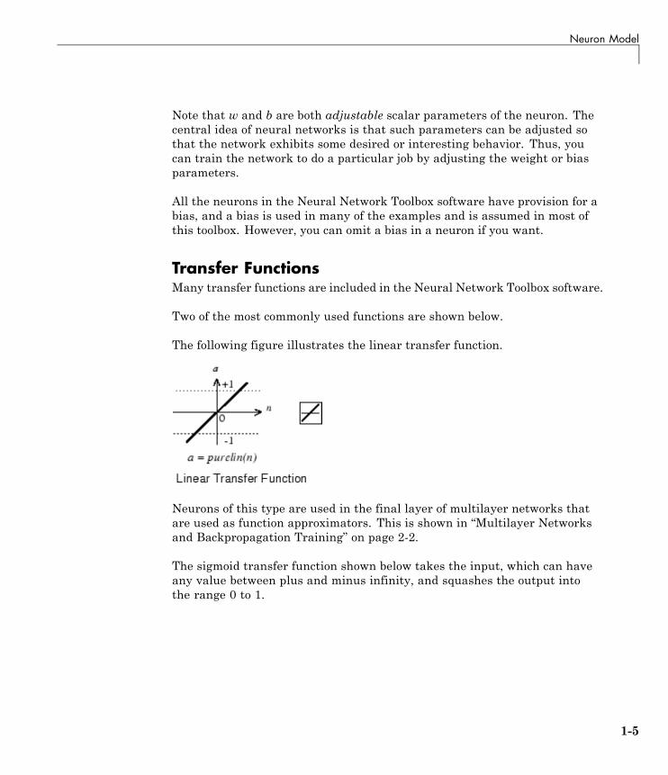
Transfer FunctionsMany transfer functions are included in the Neural Network Toolbox software.
Two of the most commonly used functions are shown below.
The following figure illustrates the linear transfer function.
Neurons of this type are used in the final layer of multilayer networks thatare used as function approximators. This is shown in “Multilayer Networksand Backpropagation Training” on page 2-2.
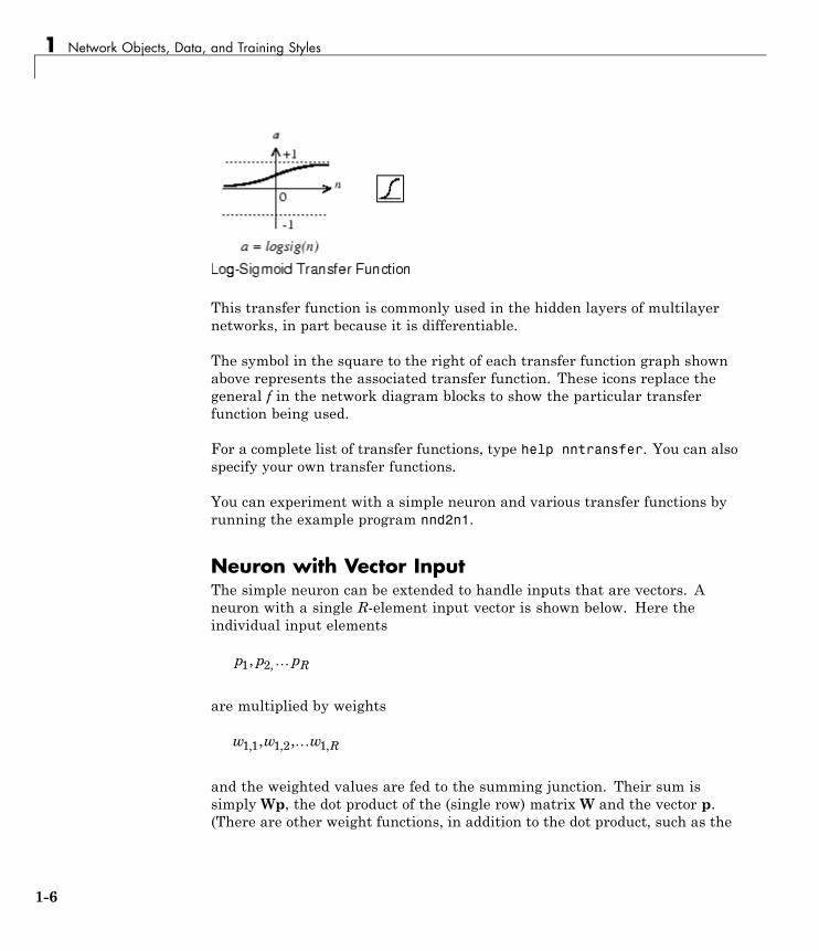
The sigmoid transfer function shown below takes the input, which can haveany value between plus and minus infinity, and squashes the output intothe range 0 to 1.
1-5
1 Network Objects, Data, and Training Styles
This transfer function is commonly used in the hidden layers of multilayernetworks, in part because it is differentiable.
The symbol in the square to the right of each transfer function graph shownabove represents the associated transfer function. These icons replace thegeneral f in the network diagram blocks to show the particular transferfunction being used.
For a complete list of transfer functions, type help nntransfer. You can alsospecify your own transfer functions.
You can experiment with a simple neuron and various transfer functions byrunning the example program nnd2n1.
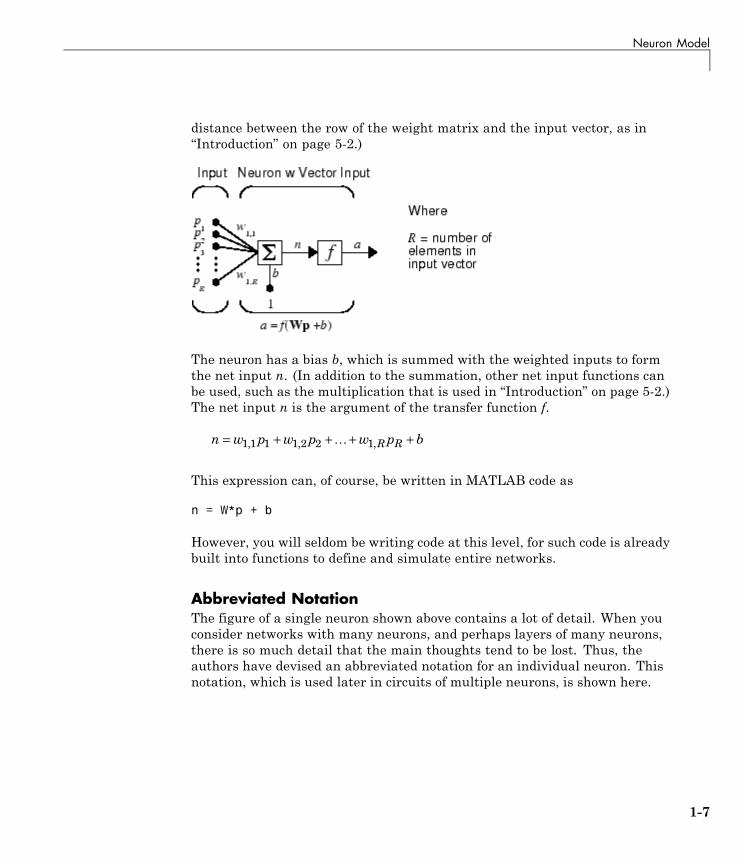
Neuron with Vector InputThe simple neuron can be extended to handle inputs that are vectors. Aneuron with a single R-element input vector is shown below. Here theindividual input elements
p p pR1 2, ,
are multiplied by weights
w w w R1 1 1 2 1, , ,, ,
and the weighted values are fed to the summing junction. Their sum issimply Wp, the dot product of the (single row) matrix W and the vector p.(There are other weight functions, in addition to the dot product, such as the
1-6
Neuron Model
distance between the row of the weight matrix and the input vector, as in“Introduction” on page 5-2.)
The neuron has a bias b, which is summed with the weighted inputs to formthe net input n. (In addition to the summation, other net input functions canbe used, such as the multiplication that is used in “Introduction” on page 5-2.)The net input n is the argument of the transfer function f.
n w p w p w p bR R= + + + +1 1 1 1 2 2 1, , ,
This expression can, of course, be written in MATLAB code as
n = W*p + b
However, you will seldom be writing code at this level, for such code is alreadybuilt into functions to define and simulate entire networks.
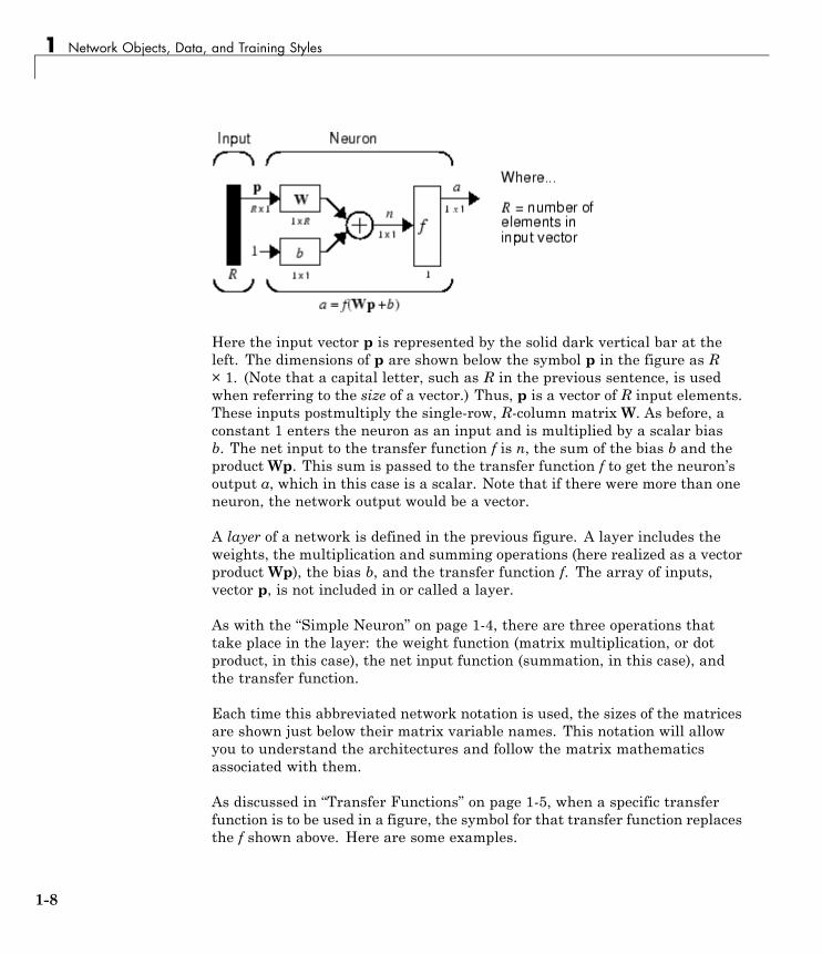
Abbreviated NotationThe figure of a single neuron shown above contains a lot of detail. When youconsider networks with many neurons, and perhaps layers of many neurons,there is so much detail that the main thoughts tend to be lost. Thus, theauthors have devised an abbreviated notation for an individual neuron. Thisnotation, which is used later in circuits of multiple neurons, is shown here.
1-7
1 Network Objects, Data, and Training Styles
Here the input vector p is represented by the solid dark vertical bar at theleft. The dimensions of p are shown below the symbol p in the figure as R× 1. (Note that a capital letter, such as R in the previous sentence, is usedwhen referring to the size of a vector.) Thus, p is a vector of R input elements.These inputs postmultiply the single-row, R-column matrix W. As before, aconstant 1 enters the neuron as an input and is multiplied by a scalar biasb. The net input to the transfer function f is n, the sum of the bias b and theproductWp. This sum is passed to the transfer function f to get the neuron’soutput a, which in this case is a scalar. Note that if there were more than oneneuron, the network output would be a vector.
A layer of a network is defined in the previous figure. A layer includes theweights, the multiplication and summing operations (here realized as a vectorproduct Wp), the bias b, and the transfer function f. The array of inputs,vector p, is not included in or called a layer.
As with the “Simple Neuron” on page 1-4, there are three operations thattake place in the layer: the weight function (matrix multiplication, or dotproduct, in this case), the net input function (summation, in this case), andthe transfer function.
Each time this abbreviated network notation is used, the sizes of the matricesare shown just below their matrix variable names. This notation will allowyou to understand the architectures and follow the matrix mathematicsassociated with them.
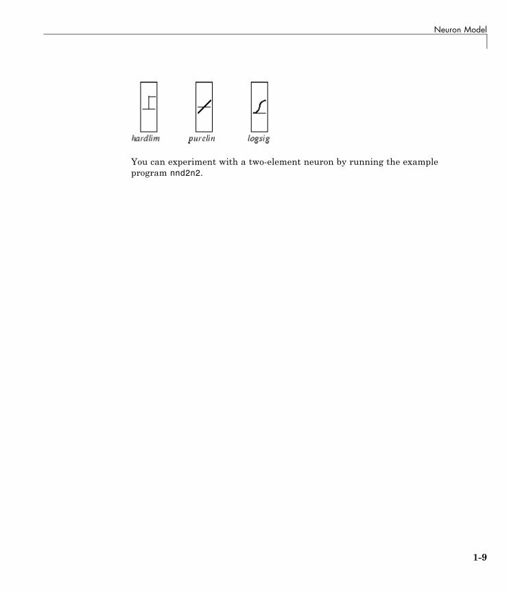
As discussed in “Transfer Functions” on page 1-5, when a specific transferfunction is to be used in a figure, the symbol for that transfer function replacesthe f shown above. Here are some examples.
1-8
Neuron Model
You can experiment with a two-element neuron by running the exampleprogram nnd2n2.
1-9
1 Network Objects, Data, and Training Styles
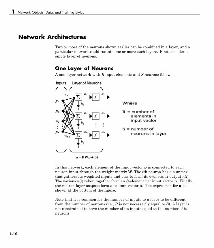
Network ArchitecturesTwo or more of the neurons shown earlier can be combined in a layer, and aparticular network could contain one or more such layers. First consider asingle layer of neurons.
One Layer of NeuronsA one-layer network with R input elements and S neurons follows.
In this network, each element of the input vector p is connected to eachneuron input through the weight matrix W. The ith neuron has a summerthat gathers its weighted inputs and bias to form its own scalar output n(i).The various n(i) taken together form an S-element net input vector n. Finally,the neuron layer outputs form a column vector a. The expression for a isshown at the bottom of the figure.
Note that it is common for the number of inputs to a layer to be differentfrom the number of neurons (i.e., R is not necessarily equal to S). A layer isnot constrained to have the number of its inputs equal to the number of itsneurons.
1-10
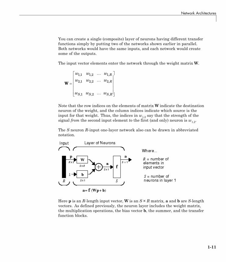
Network Architectures
You can create a single (composite) layer of neurons having different transferfunctions simply by putting two of the networks shown earlier in parallel.Both networks would have the same inputs, and each network would createsome of the outputs.
The input vector elements enter the network through the weight matrixW.
W
w w w
w w w
w w w
R
R
S S S R
1 1 1 2 1
2 1 2 2 2
1 2
, , ,
, , ,
, , ,
Note that the row indices on the elements of matrixW indicate the destinationneuron of the weight, and the column indices indicate which source is theinput for that weight. Thus, the indices in w1,2 say that the strength of thesignal from the second input element to the first (and only) neuron is w1,2.
The S neuron R-input one-layer network also can be drawn in abbreviatednotation.
Here p is an R-length input vector,W is an S × Rmatrix, a and b are S-lengthvectors. As defined previously, the neuron layer includes the weight matrix,the multiplication operations, the bias vector b, the summer, and the transferfunction blocks.
1-11
1 Network Objects, Data, and Training Styles
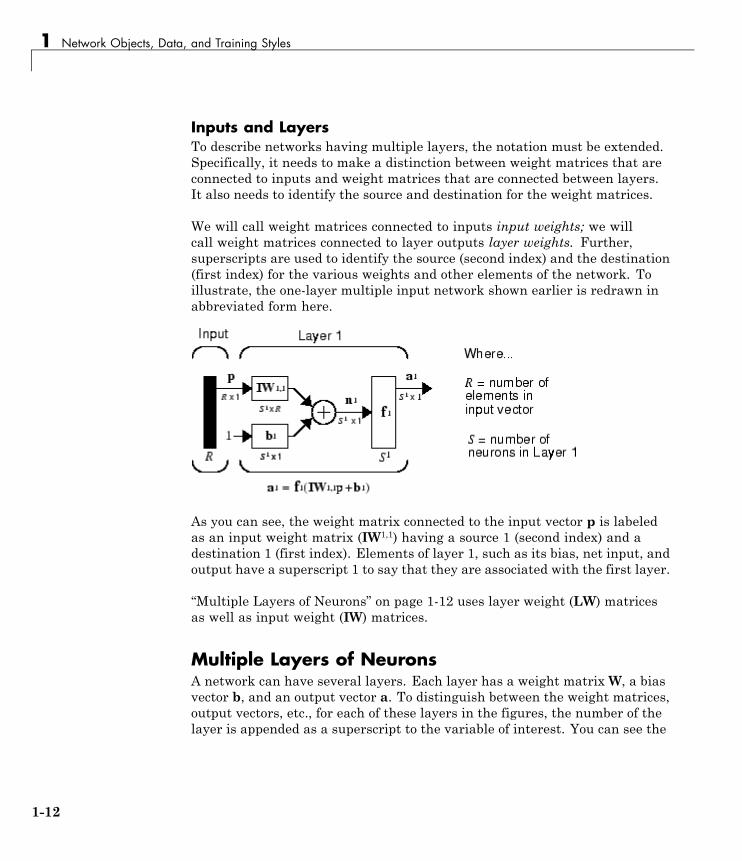
Inputs and LayersTo describe networks having multiple layers, the notation must be extended.Specifically, it needs to make a distinction between weight matrices that areconnected to inputs and weight matrices that are connected between layers.It also needs to identify the source and destination for the weight matrices.
We will call weight matrices connected to inputs input weights; we willcall weight matrices connected to layer outputs layer weights. Further,superscripts are used to identify the source (second index) and the destination(first index) for the various weights and other elements of the network. Toillustrate, the one-layer multiple input network shown earlier is redrawn inabbreviated form here.
As you can see, the weight matrix connected to the input vector p is labeledas an input weight matrix (IW1,1) having a source 1 (second index) and adestination 1 (first index). Elements of layer 1, such as its bias, net input, andoutput have a superscript 1 to say that they are associated with the first layer.
“Multiple Layers of Neurons” on page 1-12 uses layer weight (LW) matricesas well as input weight (IW) matrices.
Multiple Layers of NeuronsA network can have several layers. Each layer has a weight matrix W, a biasvector b, and an output vector a. To distinguish between the weight matrices,output vectors, etc., for each of these layers in the figures, the number of thelayer is appended as a superscript to the variable of interest. You can see the
1-12
Network Architectures
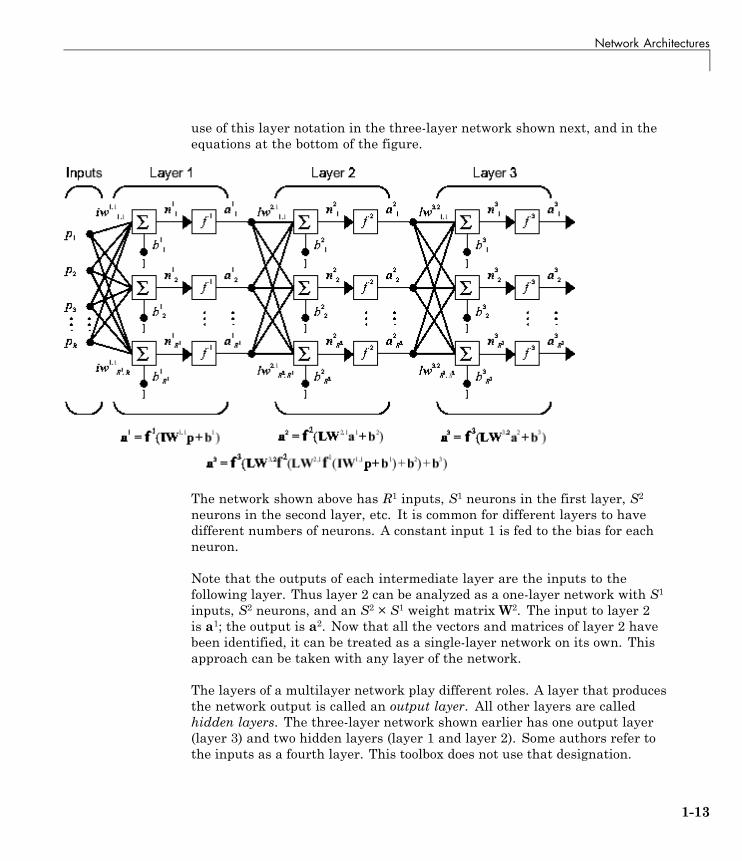
use of this layer notation in the three-layer network shown next, and in theequations at the bottom of the figure.
The network shown above has R1 inputs, S1 neurons in the first layer, S2
neurons in the second layer, etc. It is common for different layers to havedifferent numbers of neurons. A constant input 1 is fed to the bias for eachneuron.
Note that the outputs of each intermediate layer are the inputs to thefollowing layer. Thus layer 2 can be analyzed as a one-layer network with S1
inputs, S2 neurons, and an S2 × S1 weight matrix W2. The input to layer 2is a1; the output is a2. Now that all the vectors and matrices of layer 2 havebeen identified, it can be treated as a single-layer network on its own. Thisapproach can be taken with any layer of the network.
The layers of a multilayer network play different roles. A layer that producesthe network output is called an output layer. All other layers are calledhidden layers. The three-layer network shown earlier has one output layer(layer 3) and two hidden layers (layer 1 and layer 2). Some authors refer tothe inputs as a fourth layer. This toolbox does not use that designation.
1-13
1 Network Objects, Data, and Training Styles
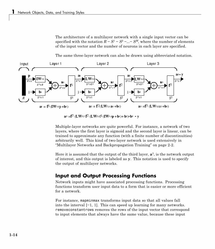
The architecture of a multilayer network with a single input vector can bespecified with the notation R − S1 − S2 −...− SM, where the number of elementsof the input vector and the number of neurons in each layer are specified.
The same three-layer network can also be drawn using abbreviated notation.
Multiple-layer networks are quite powerful. For instance, a network of twolayers, where the first layer is sigmoid and the second layer is linear, can betrained to approximate any function (with a finite number of discontinuities)arbitrarily well. This kind of two-layer network is used extensively in“Multilayer Networks and Backpropagation Training” on page 2-2.
Here it is assumed that the output of the third layer, a3, is the network outputof interest, and this output is labeled as y. This notation is used to specifythe output of multilayer networks.
Input and Output Processing FunctionsNetwork inputs might have associated processing functions. Processingfunctions transform user input data to a form that is easier or more efficientfor a network.
For instance, mapminmax transforms input data so that all values fallinto the interval [−1, 1]. This can speed up learning for many networks.removeconstantrows removes the rows of the input vector that correspondto input elements that always have the same value, because these input
1-14
Network Architectures
elements are not providing any useful information to the network. The thirdcommon processing function is fixunknowns, which recodes unknown data(represented in the user’s data with NaN values) into a numerical form for thenetwork. fixunknowns preserves information about which values are knownand which are unknown.
Similarly, network outputs can also have associated processing functions.Output processing functions are used to transform user-provided targetvectors for network use. Then, network outputs are reverse-processed usingthe same functions to produce output data with the same characteristics asthe original user-provided targets.
Both mapminmax and removeconstantrows are often associated withnetwork outputs. However, fixunknowns is not. Unknown values in targets(represented by NaN values) do not need to be altered for network use.
Processing functions are described in more detail in “Preprocessing andPostprocessing” on page 2-7.
1-15
1 Network Objects, Data, and Training Styles
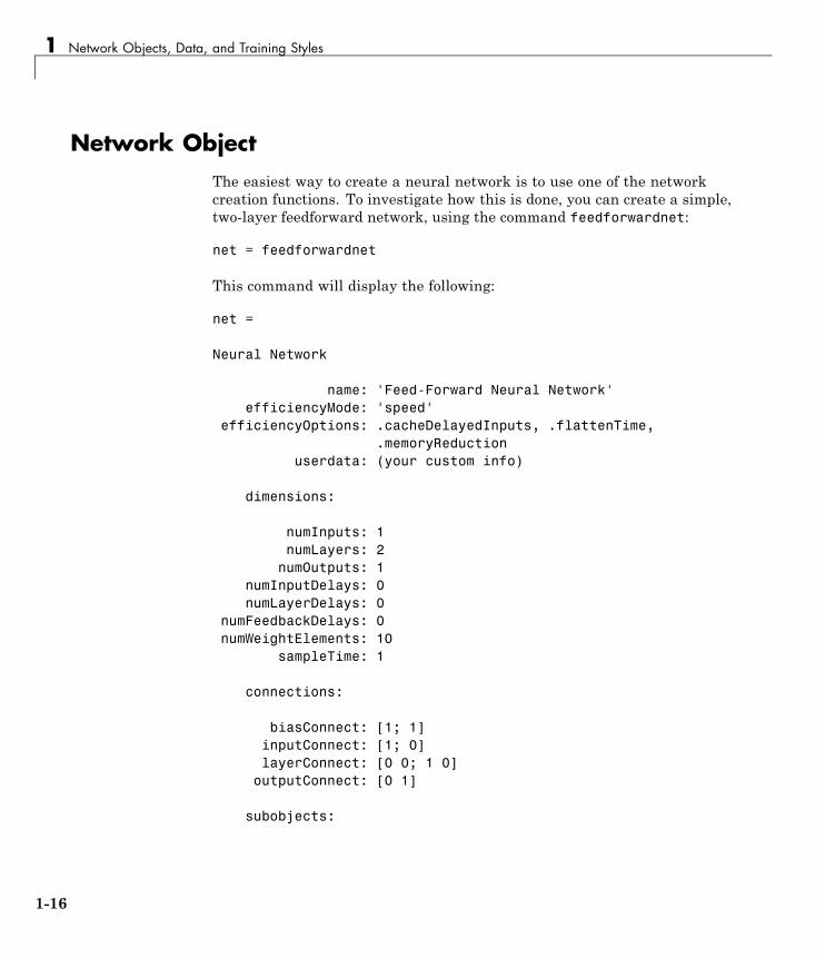
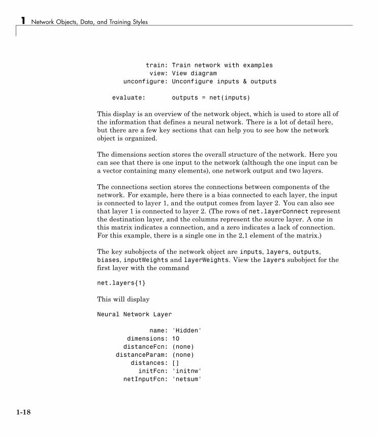
Network ObjectThe easiest way to create a neural network is to use one of the networkcreation functions. To investigate how this is done, you can create a simple,two-layer feedforward network, using the command feedforwardnet:
net = feedforwardnet
This command will display the following:
net =
Neural Network
name: 'Feed-Forward Neural Network'efficiencyMode: 'speed'
efficiencyOptions: .cacheDelayedInputs, .flattenTime,.memoryReduction
userdata: (your custom info)
dimensions:
numInputs: 1numLayers: 2
numOutputs: 1numInputDelays: 0numLayerDelays: 0
numFeedbackDelays: 0numWeightElements: 10
sampleTime: 1
connections:
biasConnect: [1; 1]inputConnect: [1; 0]layerConnect: [0 0; 1 0]
outputConnect: [0 1]
subobjects:
1-16
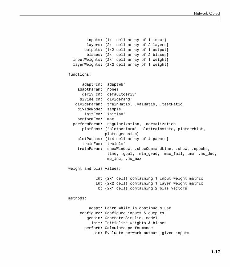
Network Object
inputs: {1x1 cell array of 1 input}layers: {2x1 cell array of 2 layers}
outputs: {1x2 cell array of 1 output}biases: {2x1 cell array of 2 biases}
inputWeights: {2x1 cell array of 1 weight}layerWeights: {2x2 cell array of 1 weight}
functions:
adaptFcn: 'adaptwb'adaptParam: (none)
derivFcn: 'defaultderiv'divideFcn: 'dividerand'
divideParam: .trainRatio, .valRatio, .testRatiodivideMode: 'sample'
initFcn: 'initlay'performFcn: 'mse'
performParam: .regularization, .normalizationplotFcns: {'plotperform', plottrainstate, ploterrhist,
plotregression}plotParams: {1x4 cell array of 4 params}
trainFcn: 'trainlm'trainParam: .showWindow, .showCommandLine, .show, .epochs,
.time, .goal, .min_grad, .max_fail, .mu, .mu_dec,
.mu_inc, .mu_max
weight and bias values:
IW: {2x1 cell} containing 1 input weight matrixLW: {2x2 cell} containing 1 layer weight matrixb: {2x1 cell} containing 2 bias vectors
methods:
adapt: Learn while in continuous useconfigure: Configure inputs & outputs
gensim: Generate Simulink modelinit: Initialize weights & biases
perform: Calculate performancesim: Evaluate network outputs given inputs
1-17
1 Network Objects, Data, and Training Styles
train: Train network with examplesview: View diagram
unconfigure: Unconfigure inputs & outputs
evaluate: outputs = net(inputs)
This display is an overview of the network object, which is used to store all ofthe information that defines a neural network. There is a lot of detail here,but there are a few key sections that can help you to see how the networkobject is organized.
The dimensions section stores the overall structure of the network. Here youcan see that there is one input to the network (although the one input can bea vector containing many elements), one network output and two layers.
The connections section stores the connections between components of thenetwork. For example, here there is a bias connected to each layer, the inputis connected to layer 1, and the output comes from layer 2. You can also seethat layer 1 is connected to layer 2. (The rows of net.layerConnect representthe destination layer, and the columns represent the source layer. A one inthis matrix indicates a connection, and a zero indicates a lack of connection.For this example, there is a single one in the 2,1 element of the matrix.)
The key subobjects of the network object are inputs, layers, outputs,biases, inputWeights and layerWeights. View the layers subobject for thefirst layer with the command
net.layers{1}
This will display
Neural Network Layer
name: 'Hidden'dimensions: 10
distanceFcn: (none)distanceParam: (none)
distances: []initFcn: 'initnw'
netInputFcn: 'netsum'
1-18
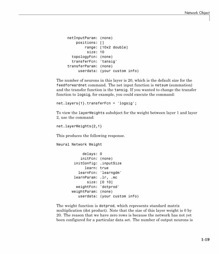
Network Object
netInputParam: (none)positions: []
range: [10x2 double]size: 10
topologyFcn: (none)transferFcn: 'tansig'
transferParam: (none)userdata: (your custom info)
The number of neurons in this layer is 20, which is the default size for thefeedforwardnet command. The net input function is netsum (summation)and the transfer function is the tansig. If you wanted to change the transferfunction to logsig, for example, you could execute the command:
net.layers{1}.transferFcn = 'logsig';
To view the layerWeights subobject for the weight between layer 1 and layer2, use the command:
net.layerWeights{2,1}
This produces the following response.
Neural Network Weight
delays: 0initFcn: (none)
initConfig: .inputSizelearn: true
learnFcn: 'learngdm'learnParam: .lr, .mc
size: [0 10]weightFcn: 'dotprod'
weightParam: (none)userdata: (your custom info)
The weight function is dotprod, which represents standard matrixmultiplication (dot product). Note that the size of this layer weight is 0 by20. The reason that we have zero rows is because the network has not yetbeen configured for a particular data set. The number of output neurons is
1-19

1 Network Objects, Data, and Training Styles
determined by the number of elements in your target vector. During theconfiguration process, you will provide the network with example inputs andtargets, and then the number of output neurons can be assigned.
This gives you some idea of how the network object is organized. For manyapplications, you will not need to be concerned about making changes directlyto the network object, since that is taken care of by the network creationfunctions. It is usually only when you want to override the system defaultsthat it is necessary to access the network object directly. Later topics willshow how this is done for particular networks and training methods.
If you would like to investigate the network object in more detail, you will findthat the object listings, such as the one shown above, contains links to helpfiles on each subobject. Just click the links, and you can selectively investigatethose parts of the object that are of interest to you.
1-20
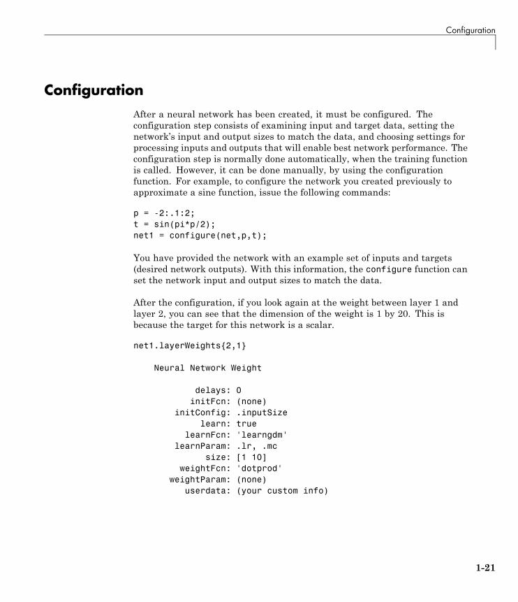
Configuration
ConfigurationAfter a neural network has been created, it must be configured. Theconfiguration step consists of examining input and target data, setting thenetwork’s input and output sizes to match the data, and choosing settings forprocessing inputs and outputs that will enable best network performance. Theconfiguration step is normally done automatically, when the training functionis called. However, it can be done manually, by using the configurationfunction. For example, to configure the network you created previously toapproximate a sine function, issue the following commands:
p = -2:.1:2;t = sin(pi*p/2);net1 = configure(net,p,t);
You have provided the network with an example set of inputs and targets(desired network outputs). With this information, the configure function canset the network input and output sizes to match the data.
After the configuration, if you look again at the weight between layer 1 andlayer 2, you can see that the dimension of the weight is 1 by 20. This isbecause the target for this network is a scalar.
net1.layerWeights{2,1}
Neural Network Weight
delays: 0initFcn: (none)
initConfig: .inputSizelearn: true
learnFcn: 'learngdm'learnParam: .lr, .mc
size: [1 10]weightFcn: 'dotprod'
weightParam: (none)userdata: (your custom info)
1-21
1 Network Objects, Data, and Training Styles
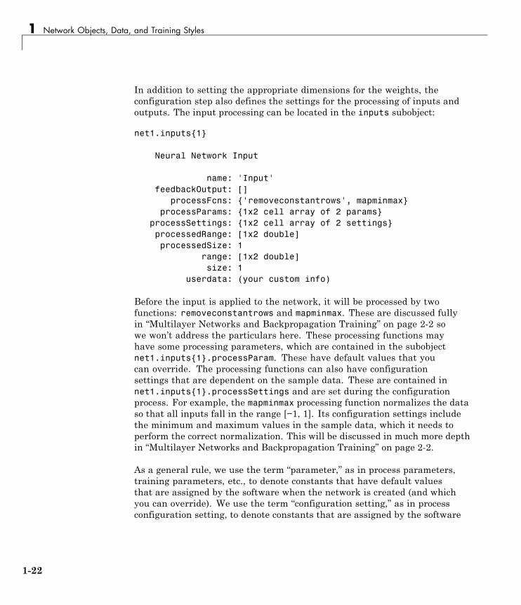
In addition to setting the appropriate dimensions for the weights, theconfiguration step also defines the settings for the processing of inputs andoutputs. The input processing can be located in the inputs subobject:
net1.inputs{1}
Neural Network Input
name: 'Input'feedbackOutput: []
processFcns: {'removeconstantrows', mapminmax}processParams: {1x2 cell array of 2 params}
processSettings: {1x2 cell array of 2 settings}processedRange: [1x2 double]processedSize: 1
range: [1x2 double]size: 1
userdata: (your custom info)
Before the input is applied to the network, it will be processed by twofunctions: removeconstantrows and mapminmax. These are discussed fullyin “Multilayer Networks and Backpropagation Training” on page 2-2 sowe won’t address the particulars here. These processing functions mayhave some processing parameters, which are contained in the subobjectnet1.inputs{1}.processParam. These have default values that youcan override. The processing functions can also have configurationsettings that are dependent on the sample data. These are contained innet1.inputs{1}.processSettings and are set during the configurationprocess. For example, the mapminmax processing function normalizes the dataso that all inputs fall in the range [−1, 1]. Its configuration settings includethe minimum and maximum values in the sample data, which it needs toperform the correct normalization. This will be discussed in much more depthin “Multilayer Networks and Backpropagation Training” on page 2-2.
As a general rule, we use the term “parameter,” as in process parameters,training parameters, etc., to denote constants that have default valuesthat are assigned by the software when the network is created (and whichyou can override). We use the term “configuration setting,” as in processconfiguration setting, to denote constants that are assigned by the software
1-22

Configuration
from an analysis of sample data. These settings do not have default values,and should not generally be overridden.
1-23
1 Network Objects, Data, and Training Styles
Data StructuresThis section discusses how the format of input data structures affects thesimulation of networks. It starts with static networks, and then continueswith dynamic networks. The following section describes how the format of thedata structures affects network training.
There are two basic types of input vectors: those that occur concurrently(at the same time, or in no particular time sequence), and those that occursequentially in time. For concurrent vectors, the order is not important, and ifthere were a number of networks running in parallel, you could present oneinput vector to each of the networks. For sequential vectors, the order inwhich the vectors appear is important.
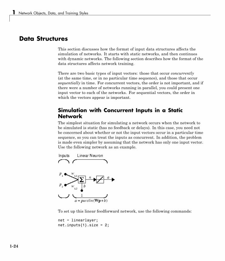
Simulation with Concurrent Inputs in a StaticNetworkThe simplest situation for simulating a network occurs when the network tobe simulated is static (has no feedback or delays). In this case, you need notbe concerned about whether or not the input vectors occur in a particular timesequence, so you can treat the inputs as concurrent. In addition, the problemis made even simpler by assuming that the network has only one input vector.Use the following network as an example.
To set up this linear feedforward network, use the following commands:
net = linearlayer;net.inputs{1}.size = 2;
1-24
Data Structures
net.layers{1}.dimensions = 1;
For simplicity, assign the weight matrix and bias to beW = [1 2] and b = [0].
The commands for these assignments are
net.IW{1,1} = [1 2];net.b{1} = 0;
Suppose that the network simulation data set consists of Q = 4 concurrentvectors:
p p p p1 2 3 412
21
23
31
=⎡
⎣⎢
⎤
⎦⎥ =
⎡
⎣⎢
⎤
⎦⎥ =
⎡
⎣⎢
⎤
⎦⎥ =
⎡
⎣⎢
⎤
⎦⎥, , ,
Concurrent vectors are presented to the network as a single matrix:
P = [1 2 2 3; 2 1 3 1];
You can now simulate the network:
A = net(P)A =
5 4 8 5
A single matrix of concurrent vectors is presented to the network, and thenetwork produces a single matrix of concurrent vectors as output. Theresult would be the same if there were four networks operating in paralleland each network received one of the input vectors and produced one of theoutputs. The ordering of the input vectors is not important, because they donot interact with each other.
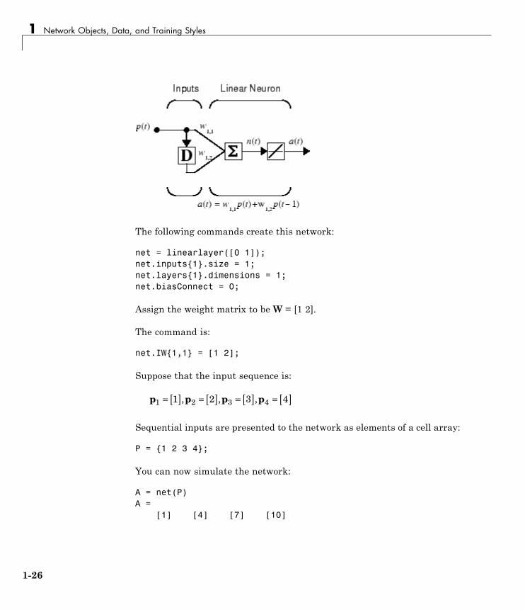
Simulation with Sequential Inputs in a DynamicNetworkWhen a network contains delays, the input to the network would normally bea sequence of input vectors that occur in a certain time order. To illustratethis case, the next figure shows a simple network that contains one delay.
1-25
1 Network Objects, Data, and Training Styles
The following commands create this network:
net = linearlayer([0 1]);net.inputs{1}.size = 1;net.layers{1}.dimensions = 1;net.biasConnect = 0;
Assign the weight matrix to be W = [1 2].
The command is:
net.IW{1,1} = [1 2];
Suppose that the input sequence is:
p p p p1 2 3 41 2 3 4= [ ] = [ ] = [ ] = [ ], , ,
Sequential inputs are presented to the network as elements of a cell array:
P = {1 2 3 4};
You can now simulate the network:
A = net(P)A =
[1] [4] [7] [10]
1-26
Data Structures
You input a cell array containing a sequence of inputs, and the networkproduces a cell array containing a sequence of outputs. The order of the inputsis important when they are presented as a sequence. In this case, the currentoutput is obtained by multiplying the current input by 1 and the precedinginput by 2 and summing the result. If you were to change the order of theinputs, the numbers obtained in the output would change.
Simulation with Concurrent Inputs in a DynamicNetworkIf you were to apply the same inputs as a set of concurrent inputs insteadof a sequence of inputs, you would obtain a completely different response.(However, it is not clear why you would want to do this with a dynamicnetwork.) It would be as if each input were applied concurrently to a separateparallel network. For the previous example, “Simulation with SequentialInputs in a Dynamic Network” on page 1-25, if you use a concurrent set ofinputs you have
p p p p1 2 3 41 2 3 4= [ ] = [ ] = [ ] = [ ], , ,
which can be created with the following code:
P = [1 2 3 4];
When you simulate with concurrent inputs, you obtain
A = net(P)A =
1 2 3 4
The result is the same as if you had concurrently applied each one of theinputs to a separate network and computed one output. Note that becauseyou did not assign any initial conditions to the network delays, they wereassumed to be 0. For this case the output is simply 1 times the input, becausethe weight that multiplies the current input is 1.
In certain special cases, you might want to simulate the network response toseveral different sequences at the same time. In this case, you would want to
1-27
1 Network Objects, Data, and Training Styles
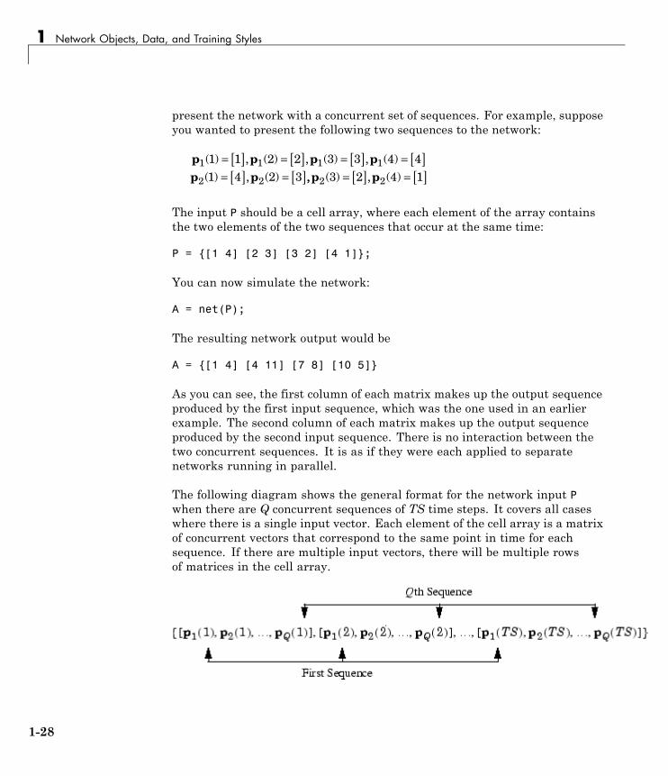
present the network with a concurrent set of sequences. For example, supposeyou wanted to present the following two sequences to the network:
p p p pp p
1 1 1 1
2 2
1 1 2 2 3 3 4 41 4 2 3( ) , ( ) , ( ) , ( )( ) , ( )
= [ ] = [ ] = [ ] = [ ]= [ ] = [ ],, ( ) , ( )p p2 23 2 4 1= [ ] = [ ]
The input P should be a cell array, where each element of the array containsthe two elements of the two sequences that occur at the same time:
P = {[1 4] [2 3] [3 2] [4 1]};
You can now simulate the network:
A = net(P);
The resulting network output would be
A = {[1 4] [4 11] [7 8] [10 5]}
As you can see, the first column of each matrix makes up the output sequenceproduced by the first input sequence, which was the one used in an earlierexample. The second column of each matrix makes up the output sequenceproduced by the second input sequence. There is no interaction between thetwo concurrent sequences. It is as if they were each applied to separatenetworks running in parallel.
The following diagram shows the general format for the network input Pwhen there are Q concurrent sequences of TS time steps. It covers all caseswhere there is a single input vector. Each element of the cell array is a matrixof concurrent vectors that correspond to the same point in time for eachsequence. If there are multiple input vectors, there will be multiple rowsof matrices in the cell array.
1-28

Data Structures
In this section, you apply sequential and concurrent inputs to dynamicnetworks. In “Simulation with Concurrent Inputs in a Static Network”on page 1-24, you applied concurrent inputs to static networks. It is alsopossible to apply sequential inputs to static networks. It does not change thesimulated response of the network, but it can affect the way in which thenetwork is trained. This will become clear in “Training Styles (Adapt andTrain)” on page 1-30.
1-29
1 Network Objects, Data, and Training Styles
Training Styles (Adapt and Train)This section describes two different styles of training. In incrementaltraining the weights and biases of the network are updated each time aninput is presented to the network. In batch training the weights and biasesare only updated after all the inputs are presented. The batch trainingmethods are generally more efficient in the MATLAB environment, and theyare emphasized in the Neural Network Toolbox software, but there someapplications where incremental training can be useful, so that paradigm isimplemented as well.
Incremental Training with adaptIncremental training can be applied to both static and dynamic networks,although it is more commonly used with dynamic networks, such as adaptivefilters. This section illustrates how incremental training is performed onboth static and dynamic networks.
Incremental Training of Static NetworksConsider again the static network used for the first example. You want totrain it incrementally, so that the weights and biases are updated after eachinput is presented. In this case you use the function adapt, and the inputsand targets are presented as sequences.
Suppose you want to train the network to create the linear function:
t p p= +2 1 2
Then for the previous inputs,
p p p p1 2 3 412
21
23
31
=⎡
⎣⎢
⎤
⎦⎥ =
⎡
⎣⎢
⎤
⎦⎥ =
⎡
⎣⎢
⎤
⎦⎥ =
⎡
⎣⎢
⎤
⎦⎥, , ,
the targets would be
t t t t1 2 3 44 5 7 7= [ ] = [ ] = [ ] = [ ], , ,
1-30
Training Styles (Adapt and Train)
For incremental training, you present the inputs and targets as sequences:
P = {[1;2] [2;1] [2;3] [3;1]};T = {4 5 7 7};
First, set up the network with zero initial weights and biases. Also, set theinitial learning rate to zero to show the effect of incremental training.
net = linearlayer(0,0);net = configure(net,P,T);net.IW{1,1} = [0 0];net.b{1} = 0;
Recall from “Simulation with Concurrent Inputs in a Static Network” on page1-24 that, for a static network, the simulation of the network produces thesame outputs whether the inputs are presented as a matrix of concurrentvectors or as a cell array of sequential vectors. However, this is not true whentraining the network. When you use the adapt function, if the inputs arepresented as a cell array of sequential vectors, then the weights are updatedas each input is presented (incremental mode). As shown in the next section,if the inputs are presented as a matrix of concurrent vectors, then the weightsare updated only after all inputs are presented (batch mode).
You are now ready to train the network incrementally.
[net,a,e,pf] = adapt(net,P,T);
The network outputs remain zero, because the learning rate is zero, and theweights are not updated. The errors are equal to the targets:
a = [0] [0] [0] [0]e = [4] [5] [7] [7]
If you now set the learning rate to 0.1 you can see how the network is adjustedas each input is presented:
net.inputWeights{1,1}.learnParam.lr = 0.1;net.biases{1,1}.learnParam.lr = 0.1;[net,a,e,pf] = adapt(net,P,T);a = [0] [2] [6] [5.8]e = [4] [3] [1] [1.2]
1-31
1 Network Objects, Data, and Training Styles
The first output is the same as it was with zero learning rate, because noupdate is made until the first input is presented. The second output isdifferent, because the weights have been updated. The weights continue to bemodified as each error is computed. If the network is capable and the learningrate is set correctly, the error is eventually driven to zero.
Incremental Training with Dynamic NetworksYou can also train dynamic networks incrementally. In fact, this would bethe most common situation.
To train the network incrementally, present the inputs and targets aselements of cell arrays. Here are the initial input Pi and the inputs P andtargets T as elements of cell arrays.
Pi = {1};P = {2 3 4};T = {3 5 7};
Take the linear network with one delay at the input, as used in a previousexample. Initialize the weights to zero and set the learning rate to 0.1.
net = linearlayer([0 1],0.1);net = configure(net,P,T);net.IW{1,1} = [0 0];net.biasConnect = 0;
You want to train the network to create the current output by summing thecurrent and the previous inputs. This is the same input sequence you usedin the previous example with the exception that you assign the first term inthe sequence as the initial condition for the delay. You can now sequentiallytrain the network using adapt.
[net,a,e,pf] = adapt(net,P,T,Pi);a = [0] [2.4] [7.98]e = [3] [2.6] [-0.98]
The first output is zero, because the weights have not yet been updated. Theweights change at each subsequent time step.
1-32
Training Styles (Adapt and Train)
Batch TrainingBatch training, in which weights and biases are only updated after all theinputs and targets are presented, can be applied to both static and dynamicnetworks. Both types of networks are discussed in this section.
Batch Training with Static NetworksBatch training can be done using either adapt or train, although train isgenerally the best option, because it typically has access to more efficienttraining algorithms. Incremental training is usually done with adapt; batchtraining is usually done with train.
For batch training of a static network with adapt, the input vectors must beplaced in one matrix of concurrent vectors.
P = [1 2 2 3; 2 1 3 1];T = [4 5 7 7];
Begin with the static network used in previous examples. The learning rateis set to 0.01.
net = linearlayer(0,0.01);net = configure(net,P,T);net.IW{1,1} = [0 0];net.b{1} = 0;
When you call adapt, it invokes trains (the default adaption function for thelinear network) and learnwh (the default learning function for the weightsand biases). trains uses Widrow-Hoff learning.
[net,a,e,pf] = adapt(net,P,T);a = 0 0 0 0e = 4 5 7 7
Note that the outputs of the network are all zero, because the weights arenot updated until all the training set has been presented. If you display theweights, you find
net.IW{1,1}ans = 0.4900 0.4100
net.b{1}
1-33
1 Network Objects, Data, and Training Styles
ans =0.2300
This is different from the result after one pass of adapt with incrementalupdating.
Now perform the same batch training using train. Because the Widrow-Hoffrule can be used in incremental or batch mode, it can be invoked by adapt ortrain. (There are several algorithms that can only be used in batch mode (e.g.,Levenberg-Marquardt), so these algorithms can only be invoked by train.)
For this case, the input vectors can be in a matrix of concurrent vectorsor in a cell array of sequential vectors. Because the network is static andbecause train always operates in batch mode, train converts any cellarray of sequential vectors to a matrix of concurrent vectors. Concurrentmode operation is used whenever possible because it has a more efficientimplementation in MATLAB code:
P = [1 2 2 3; 2 1 3 1];T = [4 5 7 7];
The network is set up in the same way.
net = linearlayer(0,0.01);net = configure(net,P,T);net.IW{1,1} = [0 0];net.b{1} = 0;
Now you are ready to train the network. Train it for only one epoch, becauseyou used only one pass of adapt. The default training function for the linearnetwork is trainb, and the default learning function for the weights andbiases is learnwh, so you should get the same results obtained using adapt inthe previous example, where the default adaption function was trains.
net.trainParam.epochs = 1;net = train(net,P,T);
If you display the weights after one epoch of training, you find
net.IW{1,1}ans = 0.4900 0.4100
1-34
Training Styles (Adapt and Train)
net.b{1}ans =
0.2300
This is the same result as the batch mode training in adapt. With staticnetworks, the adapt function can implement incremental or batch training,depending on the format of the input data. If the data is presented as amatrix of concurrent vectors, batch training occurs. If the data is presentedas a sequence, incremental training occurs. This is not true for train, whichalways performs batch training, regardless of the format of the input.
Batch Training with Dynamic NetworksTraining static networks is relatively straightforward. If you use trainthe network is trained in batch mode and the inputs are converted toconcurrent vectors (columns of a matrix), even if they are originally passed asa sequence (elements of a cell array). If you use adapt, the format of the inputdetermines the method of training. If the inputs are passed as a sequence,then the network is trained in incremental mode. If the inputs are passed asconcurrent vectors, then batch mode training is used.
With dynamic networks, batch mode training is typically done with trainonly, especially if only one training sequence exists. To illustrate this,consider again the linear network with a delay. Use a learning rate of 0.02for the training. (When using a gradient descent algorithm, you typically usea smaller learning rate for batch mode training than incremental training,because all the individual gradients are summed before determining the stepchange to the weights.)
net = linearlayer([0 1],0.02);net.inputs{1}.size = 1;net.layers{1}.dimensions = 1;net.IW{1,1} = [0 0];net.biasConnect = 0;net.trainParam.epochs = 1;Pi = {1};P = {2 3 4};T = {3 5 6};
1-35
1 Network Objects, Data, and Training Styles
You want to train the network with the same sequence used for theincremental training earlier, but this time you want to update the weightsonly after all the inputs are applied (batch mode). The network is simulatedin sequential mode, because the input is a sequence, but the weights areupdated in batch mode.
net = train(net,P,T,Pi);
The weights after one epoch of training are
net.IW{1,1}ans = 0.9000 0.6200
These are different weights than you would obtain using incremental training,where the weights would be updated three times during one pass throughthe training set. For batch training the weights are only updated once ineach epoch.
Training FeedbackThe showWindow parameter allows you to specify whether a training windowis visible when you train. The training window appears by default. Two otherparameters, showCommandLine and show, determine whether command-lineoutput is generated and the number of epochs between command-linefeedback during training. For instance, this code turns off the trainingwindow and gives you training status information every 35 epochs when thenetwork is later trained with train:
net.trainParam.showWindow = false;net.trainParam.showCommandLine = true;net.trainParam.show= 35;
Sometimes it is convenient to disable all training displays. To do that, turn offboth the training window and command-line feedback:
net.trainParam.showWindow = false;net.trainParam.showCommandLine = false;
The training window appears automatically when you train. Use thenntraintool function to manually open and close the training window.
1-36

Training Styles (Adapt and Train)
nntraintoolnntraintool('close')
1-37

1 Network Objects, Data, and Training Styles
1-38
2
Multilayer Networks andBackpropagation Training
• “Multilayer Networks and Backpropagation Training” on page 2-2
• “Multilayer Neural Network Architecture” on page 2-3
• “Collect and Prepare the Data” on page 2-7
• “Create, Configure, and Initialize the Network” on page 2-13
• “Train the Network” on page 2-15
• “Post-Training Analysis (Network Validation)” on page 2-23
• “Use the Network” on page 2-28
• “Automatic Code Generation” on page 2-29
• “Limitations and Cautions” on page 2-30
2 Multilayer Networks and Backpropagation Training
Multilayer Networks and Backpropagation TrainingThe multilayer feedforward neural network is the workhorse of the NeuralNetwork Toolbox software. It can be used for both function fitting andpattern recognition problems. With the addition of a tapped delay line, itcan also be used for prediction problems (see “Focused Time-Delay NeuralNetwork (timedelaynet)” on page 3-13). This topic shows how you can use themultilayer network. It also illustrates the basic procedures for designingany neural network.
Note The training functions described in this topic are not limited tomultilayer networks. They can be used to train arbitrary architectures (evencustom networks), as long as their components are differentiable.
The work flow for the general neural network design process has sevenprimary steps:
1 Collect data
2 Create the network
3 Configure the network
4 Initialize the weights and biases
5 Train the network
6 Validate the network (post-training analysis)
7 Use the network
Step 1 might happen outside the framework of Neural Network Toolboxsoftware, but this step is critical to the success of the design process.
2-2
Multilayer Neural Network Architecture
Multilayer Neural Network Architecture
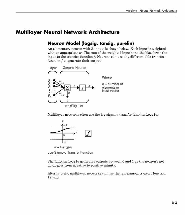
Neuron Model (logsig, tansig, purelin)An elementary neuron with R inputs is shown below. Each input is weightedwith an appropriate w. The sum of the weighted inputs and the bias forms theinput to the transfer function f. Neurons can use any differentiable transferfunction f to generate their output.
Multilayer networks often use the log-sigmoid transfer function logsig.
The function logsig generates outputs between 0 and 1 as the neuron’s netinput goes from negative to positive infinity.
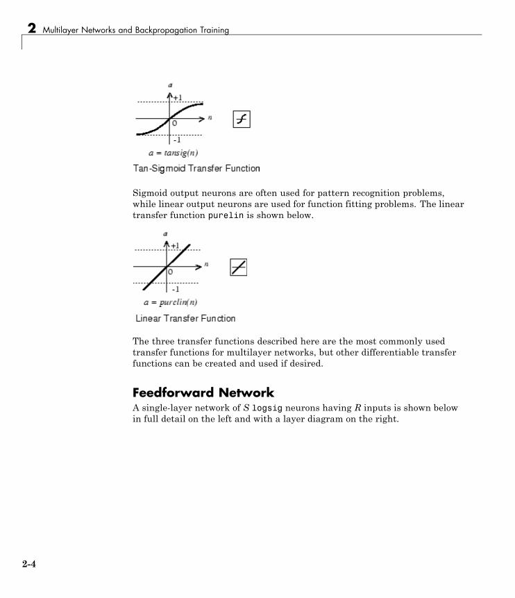
Alternatively, multilayer networks can use the tan-sigmoid transfer functiontansig.
2-3
2 Multilayer Networks and Backpropagation Training
Sigmoid output neurons are often used for pattern recognition problems,while linear output neurons are used for function fitting problems. The lineartransfer function purelin is shown below.
The three transfer functions described here are the most commonly usedtransfer functions for multilayer networks, but other differentiable transferfunctions can be created and used if desired.
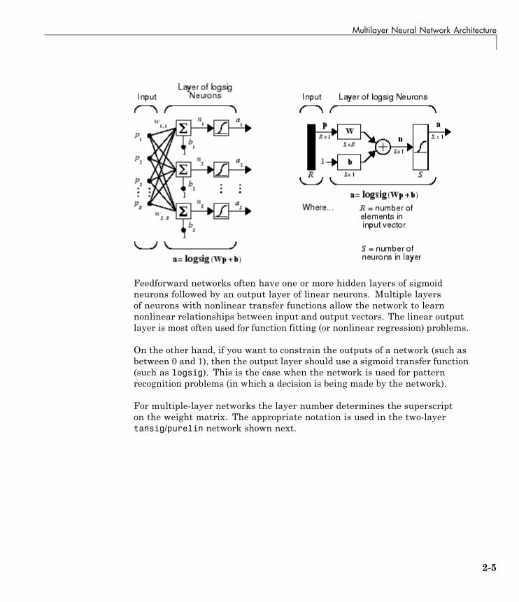
Feedforward NetworkA single-layer network of S logsig neurons having R inputs is shown belowin full detail on the left and with a layer diagram on the right.
2-4
Multilayer Neural Network Architecture
Feedforward networks often have one or more hidden layers of sigmoidneurons followed by an output layer of linear neurons. Multiple layersof neurons with nonlinear transfer functions allow the network to learnnonlinear relationships between input and output vectors. The linear outputlayer is most often used for function fitting (or nonlinear regression) problems.
On the other hand, if you want to constrain the outputs of a network (such asbetween 0 and 1), then the output layer should use a sigmoid transfer function(such as logsig). This is the case when the network is used for patternrecognition problems (in which a decision is being made by the network).
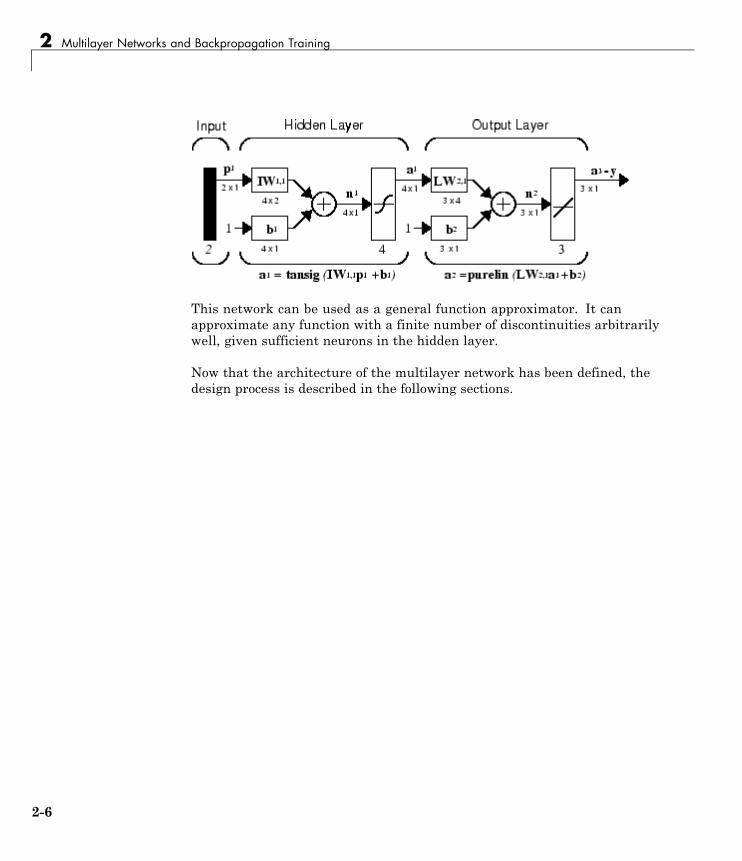
For multiple-layer networks the layer number determines the superscripton the weight matrix. The appropriate notation is used in the two-layertansig/purelin network shown next.
2-5
2 Multilayer Networks and Backpropagation Training
This network can be used as a general function approximator. It canapproximate any function with a finite number of discontinuities arbitrarilywell, given sufficient neurons in the hidden layer.
Now that the architecture of the multilayer network has been defined, thedesign process is described in the following sections.
2-6
Collect and Prepare the Data
Collect and Prepare the DataBefore beginning the network design process, you first collect and preparesample data. It is generally difficult to incorporate prior knowledge into aneural network, therefore the network can only be as accurate as the datathat are used to train the network.
It is important that the data cover the range of inputs for which the networkwill be used. Multilayer networks can be trained to generalize well within therange of inputs for which they have been trained. However, they do not havethe ability to accurately extrapolate beyond this range, so it is important thatthe training data span the full range of the input space.
After the data have been collected, there are two steps that need to beperformed before the data are used to train the network: the data need to bepreprocessed, and they need to be divided into subsets. The next two sectionsdescribe these two steps.
Preprocessing and PostprocessingNeural network training can be made more efficient if you perform certainpreprocessing steps on the network inputs and targets. This section describesseveral preprocessing routines that you can use. (The most common of theseare provided automatically when you create a network, and they become partof the network object, so that whenever the network is used, the data cominginto the network is preprocessed in the same way.)
For example, in multilayer networks, sigmoid transfer functions are generallyused in the hidden layers. These functions become essentially saturated whenthe net input is greater than three (exp (−3) 0.05). If this happens at thebeginning of the training process, the gradients will be very small, and thenetwork training will be very slow. In the first layer of the network, the netinput is a product of the input times the weight plus the bias. If the input isvery large, then the weight must be very small in order to prevent the transferfunction from becoming saturated. It is standard practice to normalize theinputs before applying them to the network.
Generally, the normalization step is applied to both the input vectors and thetarget vectors in the data set. In this way, the network output always fallsinto a normalized range. The network output can then be reverse transformed
2-7
2 Multilayer Networks and Backpropagation Training
back into the units of the original target data when the network is put touse in the field.
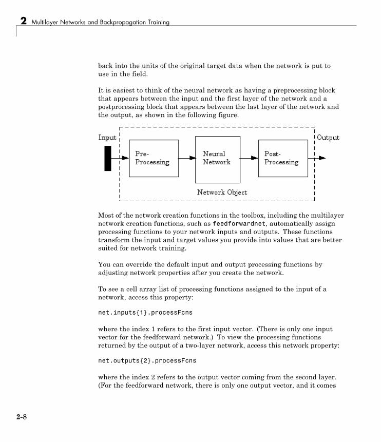
It is easiest to think of the neural network as having a preprocessing blockthat appears between the input and the first layer of the network and apostprocessing block that appears between the last layer of the network andthe output, as shown in the following figure.
Most of the network creation functions in the toolbox, including the multilayernetwork creation functions, such as feedforwardnet, automatically assignprocessing functions to your network inputs and outputs. These functionstransform the input and target values you provide into values that are bettersuited for network training.
You can override the default input and output processing functions byadjusting network properties after you create the network.
To see a cell array list of processing functions assigned to the input of anetwork, access this property:
net.inputs{1}.processFcns
where the index 1 refers to the first input vector. (There is only one inputvector for the feedforward network.) To view the processing functionsreturned by the output of a two-layer network, access this network property:
net.outputs{2}.processFcns
where the index 2 refers to the output vector coming from the second layer.(For the feedforward network, there is only one output vector, and it comes
2-8
Collect and Prepare the Data
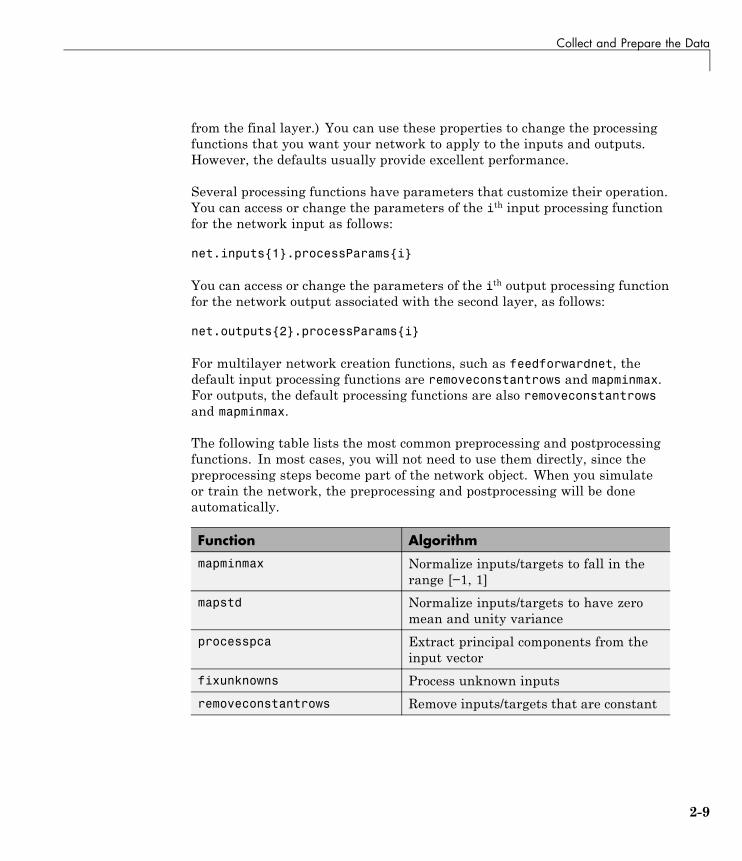
from the final layer.) You can use these properties to change the processingfunctions that you want your network to apply to the inputs and outputs.However, the defaults usually provide excellent performance.
Several processing functions have parameters that customize their operation.You can access or change the parameters of the ith input processing functionfor the network input as follows:
net.inputs{1}.processParams{i}
You can access or change the parameters of the ith output processing functionfor the network output associated with the second layer, as follows:
net.outputs{2}.processParams{i}
For multilayer network creation functions, such as feedforwardnet, thedefault input processing functions are removeconstantrows and mapminmax.For outputs, the default processing functions are also removeconstantrowsand mapminmax.
The following table lists the most common preprocessing and postprocessingfunctions. In most cases, you will not need to use them directly, since thepreprocessing steps become part of the network object. When you simulateor train the network, the preprocessing and postprocessing will be doneautomatically.
Function Algorithm
mapminmax Normalize inputs/targets to fall in therange [−1, 1]
mapstd Normalize inputs/targets to have zeromean and unity variance
processpca Extract principal components from theinput vector
fixunknowns Process unknown inputs
removeconstantrows Remove inputs/targets that are constant
2-9
2 Multilayer Networks and Backpropagation Training
Representing Unknown or Don’t Care TargetsUnknown or “don’t care” targets can be represented with NaN values. Wedo not want unknown target values to have an impact on training, but ifa network has several outputs, some elements of any target vector may beknown while others are unknown. One solution would be to remove thepartially unknown target vector and its associated input vector from thetraining set, but that involves the loss of the good target values. A bettersolution is to represent those unknown targets with NaN values. All theperformance functions of the toolbox will ignore those targets for purposes ofcalculating performance and derivatives of performance.
Dividing the DataWhen training multilayer networks, the general practice is to first dividethe data into three subsets. The first subset is the training set, which isused for computing the gradient and updating the network weights andbiases. The second subset is the validation set. The error on the validationset is monitored during the training process. The validation error normallydecreases during the initial phase of training, as does the training set error.However, when the network begins to overfit the data, the error on thevalidation set typically begins to rise. The network weights and biases aresaved at the minimum of the validation set error. This technique is discussedin more detail in “Improving Generalization” on page 8-34.
The test set error is not used during training, but it is used to comparedifferent models. It is also useful to plot the test set error during the trainingprocess. If the error on the test set reaches a minimum at a significantlydifferent iteration number than the validation set error, this might indicate apoor division of the data set.
There are four functions provided for dividing data into training, validationand test sets. They are dividerand (the default), divideblock, divideint,and divideind. The data division is normally performed automatically whenyou train the network.
Function Algorithm
dividerand Divide the data randomly (default)
divideblock Divide the data into contiguous blocks
2-10
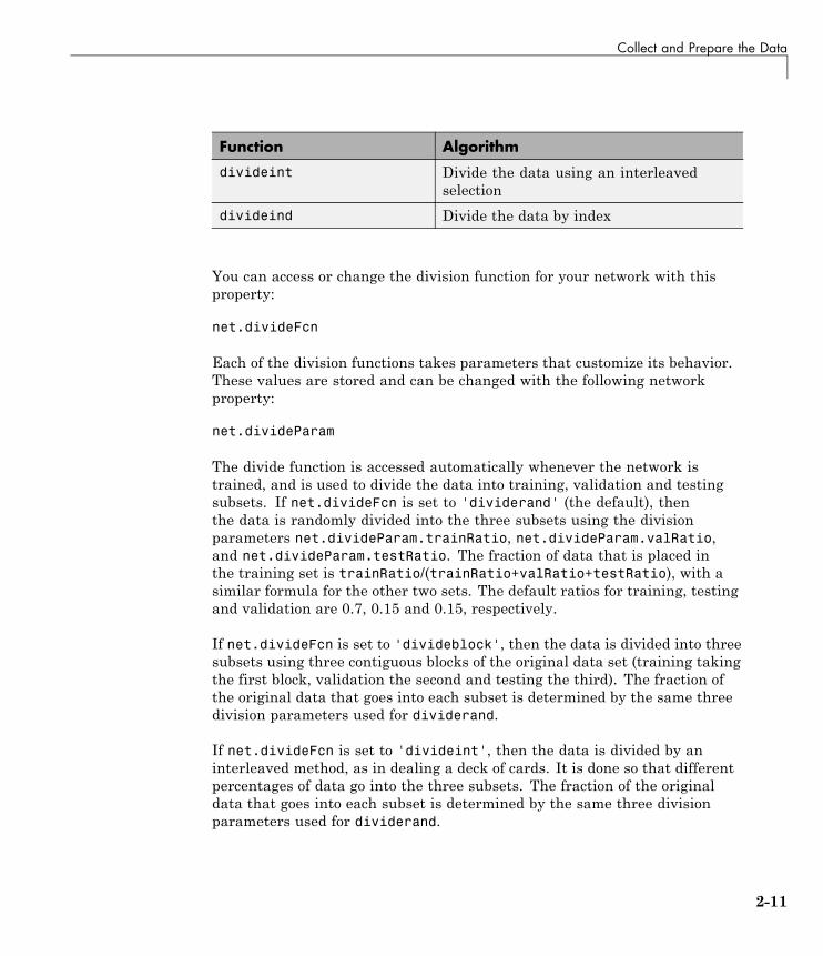
Collect and Prepare the Data
Function Algorithm
divideint Divide the data using an interleavedselection
divideind Divide the data by index
You can access or change the division function for your network with thisproperty:
net.divideFcn
Each of the division functions takes parameters that customize its behavior.These values are stored and can be changed with the following networkproperty:
net.divideParam
The divide function is accessed automatically whenever the network istrained, and is used to divide the data into training, validation and testingsubsets. If net.divideFcn is set to 'dividerand' (the default), thenthe data is randomly divided into the three subsets using the divisionparameters net.divideParam.trainRatio, net.divideParam.valRatio,and net.divideParam.testRatio. The fraction of data that is placed inthe training set is trainRatio/(trainRatio+valRatio+testRatio), with asimilar formula for the other two sets. The default ratios for training, testingand validation are 0.7, 0.15 and 0.15, respectively.
If net.divideFcn is set to 'divideblock', then the data is divided into threesubsets using three contiguous blocks of the original data set (training takingthe first block, validation the second and testing the third). The fraction ofthe original data that goes into each subset is determined by the same threedivision parameters used for dividerand.
If net.divideFcn is set to 'divideint', then the data is divided by aninterleaved method, as in dealing a deck of cards. It is done so that differentpercentages of data go into the three subsets. The fraction of the originaldata that goes into each subset is determined by the same three divisionparameters used for dividerand.
2-11

2 Multilayer Networks and Backpropagation Training
When net.divideFcn is set to 'divideind', the data is divided byindex. The indices for the three subsets are defined by the divisionparameters net.divideParam.trainInd, net.divideParam.valInd andnet.divideParam.testInd. The default assignment for these indices is thenull array, so you must set the indices when using this option.
2-12
Create, Configure, and Initialize the Network
Create, Configure, and Initialize the NetworkAfter the data has be collected, the next step in training a network is tocreate the network object. The function feedforwardnet creates a multilayerfeedforward network. If this function is invoked with no input arguments,then a default network object is created that has not been configured. Theresulting network can then be configured with the configure command.
As an example, the file housing.mat contains a predefined set of input andtarget vectors. The input vectors define data regarding real-estate propertiesand the target values define relative values of the properties. Load the datausing the following command:
load house_dataset
Loading this file creates two variables. The input matrix houseInputsconsists of 506 column vectors of 13 real estate variables for 506 differenthouses. The target matrix houseTargets consists of the corresponding 506relative valuations.
The next step is to create the network. The following call to feedforwardnetcreates a two-layer network with 10 neurons in the hidden layer. (During theconfiguration step, the number of neurons in the output layer is set to one,which is the number of elements in each vector of targets.)
net = feedforwardnet;net = configure(net,houseInputs,houseTargets);
Optional arguments can be provided to feedforwardnet. For instance, thefirst argument is an array containing the number of neurons in each hiddenlayer. (The default setting is 10, which means one hidden layer with 10neurons. One hidden layer generally produces excellent results, but youmay want to try two hidden layers, if the results with one are not adequate.Increasing the number of neurons in the hidden layer increases the power ofthe network, but requires more computation and is more likely to produceoverfitting.) The second argument contains the name of the training functionto be used. If no arguments are supplied, the default number of layers is2, the default number of neurons in the hidden layer is 10, and the defaulttraining function is trainlm. The default transfer function for hidden layersis tansig and the default for the output layer is purelin.
2-13
2 Multilayer Networks and Backpropagation Training
The configure command configures the network object and also initializesthe weights and biases of the network; therefore the network is ready fortraining. There are times when you might want to reinitialize the weights,or to perform a custom initialization. “Initializing Weights (init)” on page2-14 explains the details of the initialization process. You can also skipthe configuration step and go directly to training the network. The traincommand will automatically configure the network and initialize the weights.
Other Related ArchitecturesWhile two-layer feedforward networks can potentially learn virtually anyinput-output relationship, feedforward networks with more layers mightlearn complex relationships more quickly. For most problems, it is best tostart with two layers, and then increase to three layers, if the performancewith two layers is not satisfactory.
The function cascadeforwardnet creates cascade-forward networks. Theseare similar to feedforward networks, but include a weight connection from theinput to each layer, and from each layer to the successive layers. For example,a three-layer network has connections from layer 1 to layer 2, layer 2 to layer3, and layer 1 to layer 3. The three-layer network also has connections fromthe input to all three layers. The additional connections might improve thespeed at which the network learns the desired relationship.
The function patternnet creates a network that is very similar tofeedforwardnet, except that it uses the tansig transfer function in the lastlayer. This network is generally used for pattern recognition. Other networkscan learn dynamic or time-series relationships.
Initializing Weights (init)Before training a feedforward network, you must initialize the weights andbiases. The configure command automatically initializes the weights, butyou might want to reinitialize them. You do this with the init command.This function takes a network object as input and returns a network objectwith all weights and biases initialized. Here is how a network is initialized(or reinitialized):
net = init(net);
2-14
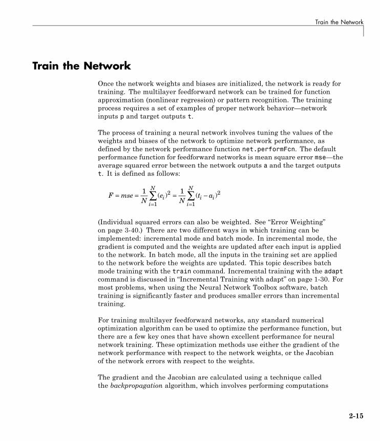
Train the Network
Train the NetworkOnce the network weights and biases are initialized, the network is ready fortraining. The multilayer feedforward network can be trained for functionapproximation (nonlinear regression) or pattern recognition. The trainingprocess requires a set of examples of proper network behavior—networkinputs p and target outputs t.
The process of training a neural network involves tuning the values of theweights and biases of the network to optimize network performance, asdefined by the network performance function net.performFcn. The defaultperformance function for feedforward networks is mean square error mse—theaverage squared error between the network outputs a and the target outputst. It is defined as follows:
F mseN
eN
t aii
N
i ii
N= = = −
= =∑ ∑1 12
1
2
1
( ) ( )
(Individual squared errors can also be weighted. See “Error Weighting”on page 3-40.) There are two different ways in which training can beimplemented: incremental mode and batch mode. In incremental mode, thegradient is computed and the weights are updated after each input is appliedto the network. In batch mode, all the inputs in the training set are appliedto the network before the weights are updated. This topic describes batchmode training with the train command. Incremental training with the adaptcommand is discussed in “Incremental Training with adapt” on page 1-30. Formost problems, when using the Neural Network Toolbox software, batchtraining is significantly faster and produces smaller errors than incrementaltraining.
For training multilayer feedforward networks, any standard numericaloptimization algorithm can be used to optimize the performance function, butthere are a few key ones that have shown excellent performance for neuralnetwork training. These optimization methods use either the gradient of thenetwork performance with respect to the network weights, or the Jacobianof the network errors with respect to the weights.
The gradient and the Jacobian are calculated using a technique calledthe backpropagation algorithm, which involves performing computations
2-15
2 Multilayer Networks and Backpropagation Training
backward through the network. The backpropagation computation is derivedusing the chain rule of calculus and is described in Chapters 11 (for thegradient) and 12 (for the Jacobian) of [HDB96].
Training AlgorithmsAs an illustration of how the training works, consider the simplestoptimization algorithm — gradient descent. It updates the network weightsand biases in the direction in which the performance function decreases mostrapidly, the negative of the gradient. One iteration of this algorithm canbe written as
x x gk k k k+ = −1
where xk is a vector of current weights and biases, gk is the current gradient,and αk is the learning rate. This equation is iterated until the networkconverges.
A list of the training algorithms that are available in the Neural NetworkToolbox software and that use gradient- or Jacobian-based methods, is shownin the following table.
For a detailed description of several of these techniques, see also Hagan,M.T., H.B. Demuth, and M.H. Beale, Neural Network Design, Boston, MA:PWS Publishing, 1996, Chapters 11 and 12.
Function Algorithm
trainlm Levenberg-Marquardt
trainbr Bayesian Regularization
trainbfg BFGS Quasi-Newton
trainrp Resilient Backpropagation
trainscg Scaled Conjugate Gradient
traincgb Conjugate Gradient with Powell/BealeRestarts
traincgf Fletcher-Powell Conjugate Gradient
traincgp Polak-Ribiére Conjugate Gradient
2-16
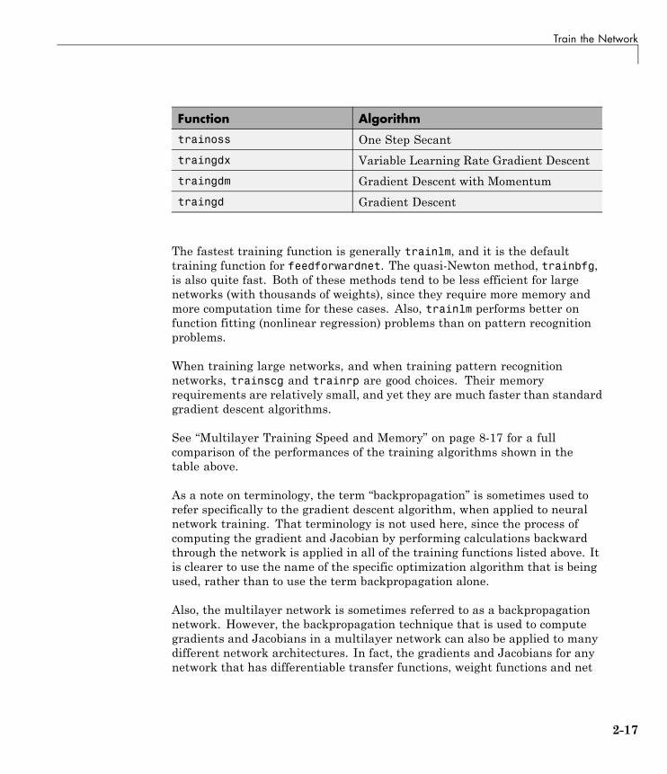
Train the Network
Function Algorithm
trainoss One Step Secant
traingdx Variable Learning Rate Gradient Descent
traingdm Gradient Descent with Momentum
traingd Gradient Descent
The fastest training function is generally trainlm, and it is the defaulttraining function for feedforwardnet. The quasi-Newton method, trainbfg,is also quite fast. Both of these methods tend to be less efficient for largenetworks (with thousands of weights), since they require more memory andmore computation time for these cases. Also, trainlm performs better onfunction fitting (nonlinear regression) problems than on pattern recognitionproblems.
When training large networks, and when training pattern recognitionnetworks, trainscg and trainrp are good choices. Their memoryrequirements are relatively small, and yet they are much faster than standardgradient descent algorithms.
See “Multilayer Training Speed and Memory” on page 8-17 for a fullcomparison of the performances of the training algorithms shown in thetable above.
As a note on terminology, the term “backpropagation” is sometimes used torefer specifically to the gradient descent algorithm, when applied to neuralnetwork training. That terminology is not used here, since the process ofcomputing the gradient and Jacobian by performing calculations backwardthrough the network is applied in all of the training functions listed above. Itis clearer to use the name of the specific optimization algorithm that is beingused, rather than to use the term backpropagation alone.
Also, the multilayer network is sometimes referred to as a backpropagationnetwork. However, the backpropagation technique that is used to computegradients and Jacobians in a multilayer network can also be applied to manydifferent network architectures. In fact, the gradients and Jacobians for anynetwork that has differentiable transfer functions, weight functions and net
2-17
2 Multilayer Networks and Backpropagation Training
input functions can be computed using the Neural Network Toolbox softwarethrough a backpropagation process. You can even create your own customnetworks and then train them using any of the training functions in the tableabove. The gradients and Jacobians will be automatically computed for you.
Efficiency and Memory ReductionThere are some network parameters that are helpful when training largenetworks or using large data sets. For example, the parameter
net.efficiency.memoryReduction
can be used to reduce the amount of memory that you use while trainingor simulating the network. If this parameter is set to 1 (the default), themaximum memory is used, and the fastest training times will be achieved.If this parameter is set to 2, then the data is divided into two parts. Allcalculations (like gradients and Jacobians) are done first on part one, andthen later on part two. Any intermediate variables used in part 1 are releasedbefore the part 2 calculations are done. This can save significant memory,especially for the trainlm training function. If memoryReduction is set to N,then the data is divided into N parts, which are computed separately. Thelarger the value of N, the larger the reduction in memory use, although theamount of reduction diminishes as N is increased.
There is a drawback to using memory reduction. A computational overhead isassociated with computing the Jacobian and gradient in submatrices. If youhave enough memory available, then it is better to leave memoryReductionset to 1 and to compute the full Jacobian or gradient in one step. If you have alarge training set, and you are running out of memory, then you should setmemoryReduction to 2 and try again. If you still run out of memory, continueto increase memoryReduction.
GeneralizationProperly trained multilayer networks tend to give reasonable answers whenpresented with inputs that they have never seen. Typically, a new input leadsto an accurate ouput, if the new input is similar to inputs used in the trainingset. This generalization property makes it possible to train a network on arepresentative set of input/target pairs and get good results without trainingthe network on all possible input/output pairs. There are two features of
2-18
Train the Network
the Neural Network Toolbox software that are designed to improve networkgeneralization: regularization and early stopping. These features and theiruse are discussed in detail in “Improving Generalization” on page 8-34. A fewcomments on using these techniques are given in the following.
The default generalization feature for the multilayer feedforward network isearly stopping. Data are automatically divided into training, validation andtest sets, as described in “Dividing the Data” on page 2-10. The error on thevalidation set is monitored during training, and the training is stopped whenthe validation increases over net.trainParam.max_fail iterations. If youwish to disable early stopping, you can assign no data to the validation set.This can be done by setting net.divideParam.valRatio to zero.
An alternative method for improving generalization is regularization.Regularization can be done automatically by using the Bayesianregularization training function trainbr. This can be done by settingnet.trainFcn to 'trainbr'. This will also automatically move any data inthe validation set to the training set.
Training ExampleTo illustrate the training process, execute the following commands:
load house_datasetnet = feedforwardnet(20);[net,tr] = train(net,houseInputs,houseTargets);
Notice that you did not need to issue the configure command, because theconfiguration is done automatically by the train function. The trainingwindow will appear during training, as shown in the following figure. (Ifyou do not want to have this window displayed during training, you can setthe parameter net.trainParam.showWindow to false. If you want traininginformation displayed in the command line, you can set the parameternet.trainParam.showCommandLine to true.)
This window shows that the data has been divided using the dividerandfunction, and the Levenberg-Marquardt (trainlm) training method has beenused with the mean square error performance function. Recall that these arethe default settings for feedforwardnet.
2-19
2 Multilayer Networks and Backpropagation Training
During training, the progress is constantly updated in the training window.Of most interest are the performance, the magnitude of the gradient ofperformance and the number of validation checks. The magnitude of thegradient and the number of validation checks are used to terminate thetraining. The gradient will become very small as the training reaches aminimum of the performance. If the magnitude of the gradient is lessthan 1e-5, the training will stop. This limit can be adjusted by settingthe parameter net.trainParam.min_grad. The number of validationchecks represents the number of successive iterations that the validationperformance fails to decrease. If this number reaches 6 (the default value),the training will stop. In this run, you can see that the training did stopbecause of the number of validation checks. You can change this criterion bysetting the parameter net.trainParam.max_fail. (Note that your resultsmay be different than those shown in the following figure, because of therandom setting of the initial weights and biases.)
2-20
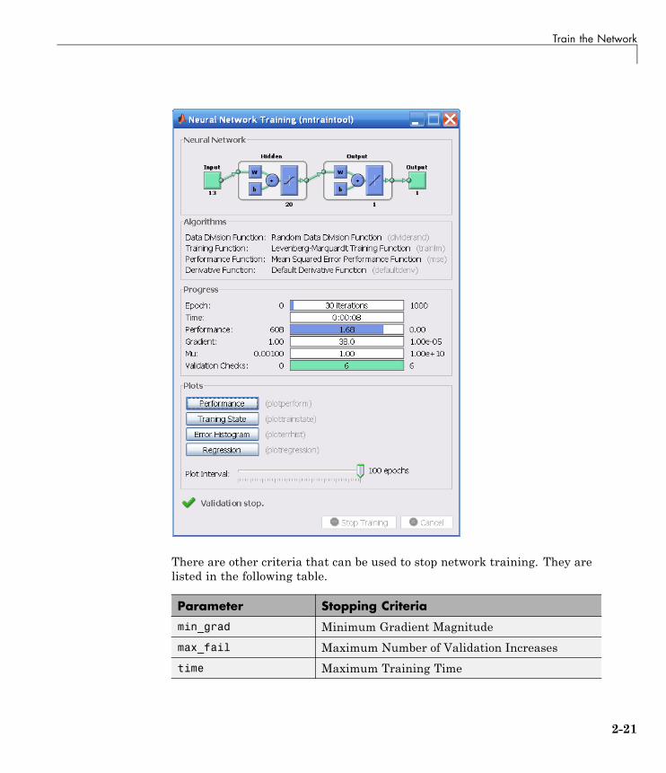
Train the Network
There are other criteria that can be used to stop network training. They arelisted in the following table.
Parameter Stopping Criteria
min_grad Minimum Gradient Magnitude
max_fail Maximum Number of Validation Increases
time Maximum Training Time
2-21
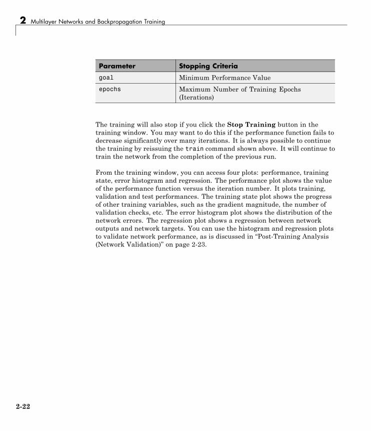
2 Multilayer Networks and Backpropagation Training
Parameter Stopping Criteria
goal Minimum Performance Value
epochs Maximum Number of Training Epochs(Iterations)
The training will also stop if you click the Stop Training button in thetraining window. You may want to do this if the performance function fails todecrease significantly over many iterations. It is always possible to continuethe training by reissuing the train command shown above. It will continue totrain the network from the completion of the previous run.
From the training window, you can access four plots: performance, trainingstate, error histogram and regression. The performance plot shows the valueof the performance function versus the iteration number. It plots training,validation and test performances. The training state plot shows the progressof other training variables, such as the gradient magnitude, the number ofvalidation checks, etc. The error histogram plot shows the distribution of thenetwork errors. The regression plot shows a regression between networkoutputs and network targets. You can use the histogram and regression plotsto validate network performance, as is discussed in “Post-Training Analysis(Network Validation)” on page 2-23.
2-22
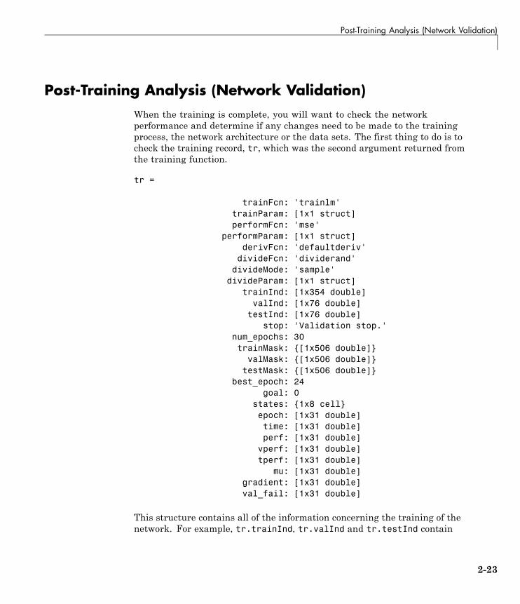
Post-Training Analysis (Network Validation)
Post-Training Analysis (Network Validation)When the training is complete, you will want to check the networkperformance and determine if any changes need to be made to the trainingprocess, the network architecture or the data sets. The first thing to do is tocheck the training record, tr, which was the second argument returned fromthe training function.
tr =
trainFcn: 'trainlm'trainParam: [1x1 struct]performFcn: 'mse'
performParam: [1x1 struct]derivFcn: 'defaultderiv'
divideFcn: 'dividerand'divideMode: 'sample'
divideParam: [1x1 struct]trainInd: [1x354 double]
valInd: [1x76 double]testInd: [1x76 double]
stop: 'Validation stop.'num_epochs: 30trainMask: {[1x506 double]}
valMask: {[1x506 double]}testMask: {[1x506 double]}
best_epoch: 24goal: 0
states: {1x8 cell}epoch: [1x31 double]time: [1x31 double]perf: [1x31 double]
vperf: [1x31 double]tperf: [1x31 double]
mu: [1x31 double]gradient: [1x31 double]val_fail: [1x31 double]
This structure contains all of the information concerning the training of thenetwork. For example, tr.trainInd, tr.valInd and tr.testInd contain
2-23
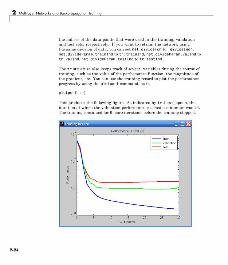
2 Multilayer Networks and Backpropagation Training
the indices of the data points that were used in the training, validationand test sets, respectively. If you want to retrain the network usingthe same division of data, you can set net.divideFcn to 'divideInd',net.divideParam.trainInd to tr.trainInd, net.divideParam.valInd totr.valInd, net.divideParam.testInd to tr.testInd.
The tr structure also keeps track of several variables during the course oftraining, such as the value of the performance function, the magnitude ofthe gradient, etc. You can use the training record to plot the performanceprogress by using the plotperf command, as in
plotperf(tr)
This produces the following figure. As indicated by tr.best_epoch, theiteration at which the validation performance reached a minimum was 24.The training continued for 6 more iterations before the training stopped.
2-24
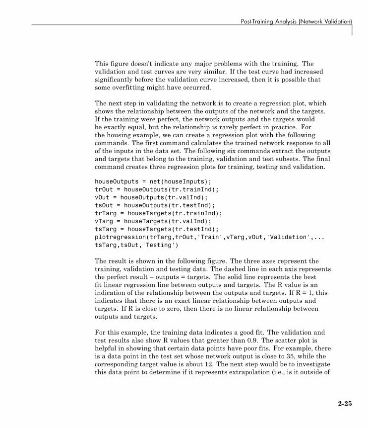
Post-Training Analysis (Network Validation)
This figure doesn’t indicate any major problems with the training. Thevalidation and test curves are very similar. If the test curve had increasedsignificantly before the validation curve increased, then it is possible thatsome overfitting might have occurred.
The next step in validating the network is to create a regression plot, whichshows the relationship between the outputs of the network and the targets.If the training were perfect, the network outputs and the targets wouldbe exactly equal, but the relationship is rarely perfect in practice. Forthe housing example, we can create a regression plot with the followingcommands. The first command calculates the trained network response to allof the inputs in the data set. The following six commands extract the outputsand targets that belong to the training, validation and test subsets. The finalcommand creates three regression plots for training, testing and validation.
houseOutputs = net(houseInputs);trOut = houseOutputs(tr.trainInd);vOut = houseOutputs(tr.valInd);tsOut = houseOutputs(tr.testInd);trTarg = houseTargets(tr.trainInd);vTarg = houseTargets(tr.valInd);tsTarg = houseTargets(tr.testInd);plotregression(trTarg,trOut,'Train',vTarg,vOut,'Validation',...tsTarg,tsOut,'Testing')
The result is shown in the following figure. The three axes represent thetraining, validation and testing data. The dashed line in each axis representsthe perfect result – outputs = targets. The solid line represents the bestfit linear regression line between outputs and targets. The R value is anindication of the relationship between the outputs and targets. If R = 1, thisindicates that there is an exact linear relationship between outputs andtargets. If R is close to zero, then there is no linear relationship betweenoutputs and targets.
For this example, the training data indicates a good fit. The validation andtest results also show R values that greater than 0.9. The scatter plot ishelpful in showing that certain data points have poor fits. For example, thereis a data point in the test set whose network output is close to 35, while thecorresponding target value is about 12. The next step would be to investigatethis data point to determine if it represents extrapolation (i.e., is it outside of
2-25
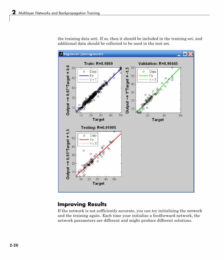
2 Multilayer Networks and Backpropagation Training
the training data set). If so, then it should be included in the training set, andadditional data should be collected to be used in the test set.
Improving ResultsIf the network is not sufficiently accurate, you can try initializing the networkand the training again. Each time your initialize a feedforward network, thenetwork parameters are different and might produce different solutions.
2-26
Post-Training Analysis (Network Validation)
net = init(net);net = train(net,houseInputs,houseTargets);
As a second approach, you can increase the number of hidden neurons above20. Larger numbers of neurons in the hidden layer give the network moreflexibility because the network has more parameters it can optimize. (Increasethe layer size gradually. If you make the hidden layer too large, you mightcause the problem to be under-characterized and the network must optimizemore parameters than there are data vectors to constrain these parameters.)
A third option is to try a different training function. Bayesian regularizationtraining with trainbr, for example, can sometimes produce bettergeneralization capability than using early stopping.
Finally, try using additional training data. Providing additional data for thenetwork is more likely to produce a network that generalizes well to new data.
2-27
2 Multilayer Networks and Backpropagation Training
Use the NetworkAfter the network is trained and validated, the network object can be used tocalculate the network response to any input. For example, if you want to findthe network response to the fifth input vector in the building data set, youcan use the following
a = net(houseInputs(:,5))a =
34.3922
If you try this command, your output might be different, depending on thestate of your random number generator when the network was initialized.Below, the network object is called to calculate the outputs for a concurrentset of all the input vectors in the housing data set. This is the batch modeform of simulation, in which all the input vectors are placed in one matrix.This is much more efficient than presenting the vectors one at a time.
a = net(houseInputs);
2-28
Automatic Code Generation
Automatic Code GenerationIt is often easiest to learn how to use the Neural Network Toolbox software bystarting with some example code and modifying it to suit your problem. It isvery simple to create example code by using the GUIs described in “GettingStarted with Neural Network Toolbox”. In particular, to generate somesample code to reproduce the function fitting examples shown in this topic,you can run the neural fitting GUI, nftool. Select the house pricing data fromthe GUI, and after you have trained the network, click the Advanced Scriptbutton on the final pane of the GUI. This will automatically generate codethat will show most of the options that are available to you when followingthe general network design process for function fitting problems. You cancustomize the generated script to fit your needs.
If you are interested in using a multilayer neural network for patternrecognition, use the pattern recognition GUI, nprtool. It will lead youthrough a similar set of design steps for pattern recognition problems, andcan then generate example code showing the options that are available forpattern recognition networks.
2-29
2 Multilayer Networks and Backpropagation Training
Limitations and CautionsYou would normally use Levenberg-Marquardt training for small and mediumsize networks, if you have enough memory available. If memory is a problem,then there are a variety of other fast algorithms available. For large networksyou will probably want to use trainscg or trainrp.
Multilayer networks are capable of performing just about any linear ornonlinear computation, and they can approximate any reasonable functionarbitrarily well. However, while the network being trained might theoreticallybe capable of performing correctly, backpropagation and its variations mightnot always find a solution. See page 12-8 of [HDB96] for a discussion ofconvergence to local minimum points.
The error surface of a nonlinear network is more complex than the errorsurface of a linear network. To understand this complexity, see the figureson pages 12-5 to 12-7 of [HDB96], which show three different error surfacesfor a multilayer network. The problem is that nonlinear transfer functions inmultilayer networks introduce many local minima in the error surface. Asgradient descent is performed on the error surface, depending on the initialstarting conditions, it is possible for the network solution to become trappedin one of these local minima. Settling in a local minimum can be good or baddepending on how close the local minimum is to the global minimum and howlow an error is required. In any case, be cautioned that although a multilayerbackpropagation network with enough neurons can implement just about anyfunction, backpropagation does not always find the correct weights for theoptimum solution. You might want to reinitialize the network and retrainseveral times to guarantee that you have the best solution.
Networks are also sensitive to the number of neurons in their hidden layers.Too few neurons can lead to underfitting. Too many neurons can contribute tooverfitting, in which all training points are well fitted, but the fitting curveoscillates wildly between these points. Ways of dealing with various of theseissues are discussed in “Improving Generalization” on page 8-34. This topic isalso discussed starting on page 11-21 of [HDB96].
2-30
3
Dynamic Networks
• “Introduction” on page 3-2
• “Focused Time-Delay Neural Network (timedelaynet)” on page 3-13
• “Preparing Data (preparets)” on page 3-18
• “Distributed Time-Delay Neural Network (distdelaynet)” on page 3-20
• “NARX Network (narxnet, closeloop)” on page 3-23
• “Layer-Recurrent Network (layrecnet)” on page 3-29
• “Training Custom Networks” on page 3-31
• “Multiple Sequences, Time-Series Utilities, and Error Weighting” on page3-37
3 Dynamic Networks
IntroductionNeural networks can be classified into dynamic and static categories. Static(feedforward) networks have no feedback elements and contain no delays; theoutput is calculated directly from the input through feedforward connections.In dynamic networks, the output depends not only on the current input to thenetwork, but also on the current or previous inputs, outputs, or states ofthe network.
The training of dynamic networks is very similar to the training ofstatic feedforward networks, as discussed in “Multilayer Networks andBackpropagation Training” on page 2-2. As described in that topic, the workflow for the general neural network design process has seven primary steps.(Data collection in step 1, while important, generally occurs outside theMATLAB environment.)
1 Collect data
2 Create the network
3 Configure the network
4 Initialize the weights and biases
5 Train the network
6 Validate the network (post-training analysis)
7 Use the network
These design steps, and all of the training methods discussed in “MultilayerNetworks and Backpropagation Training” on page 2-2, can also be used fordynamic networks. The main differences in the design process occur becausethe inputs to the dynamic networks are time sequences. (See “Simulation withSequential Inputs in a Dynamic Network” on page 1-25 and “Batch Trainingwith Dynamic Networks” on page 1-35 for discussions of simulation andtraining of dynamic networks.) This results in some additional initializationprocedures prior to training or simulating a dynamic network. There are alsospecial validation procedures that can be used for dynamic networks. (Thesewere discussed in “Time Series Prediction”.)
3-2
Introduction
This topic begins by explaining how dynamic networks operate and by givingexamples of applications for dynamic networks. Then it introduces thegeneral framework for representing dynamic networks in the toolbox. Thisallows you to design your own specialized dynamic networks, which can thenbe trained using existing toolbox training functions. Next, the topic describesseveral standard dynamic network architectures that you can create with asingle command. Each is shown with a practical application. Finally, thetopic provides an example of creating and training a custom network.
Examples of Dynamic NetworksDynamic networks can be divided into two categories: those thathave only feedforward connections, and those that have feedback, orrecurrent, connections. To understand the differences between static,feedforward-dynamic, and recurrent-dynamic networks, create some networksand see how they respond to an input sequence. (First, you might want toreview “Simulation with Sequential Inputs in a Dynamic Network” on page1-25.)
The following command creates a pulse input sequence and plots it:
p = {0 0 1 1 1 1 0 0 0 0 0 0};stem(cell2mat(p))
The next figure show the resulting pulse.
3-3
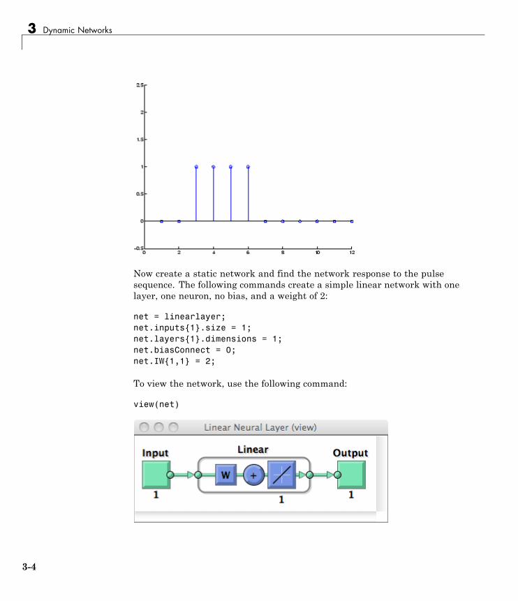
3 Dynamic Networks
Now create a static network and find the network response to the pulsesequence. The following commands create a simple linear network with onelayer, one neuron, no bias, and a weight of 2:
net = linearlayer;net.inputs{1}.size = 1;net.layers{1}.dimensions = 1;net.biasConnect = 0;net.IW{1,1} = 2;
To view the network, use the following command:
view(net)
3-4
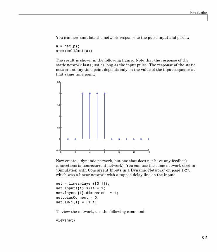
Introduction
You can now simulate the network response to the pulse input and plot it:
a = net(p);stem(cell2mat(a))
The result is shown in the following figure. Note that the response of thestatic network lasts just as long as the input pulse. The response of the staticnetwork at any time point depends only on the value of the input sequence atthat same time point.
Now create a dynamic network, but one that does not have any feedbackconnections (a nonrecurrent network). You can use the same network used in“Simulation with Concurrent Inputs in a Dynamic Network” on page 1-27,which was a linear network with a tapped delay line on the input:
net = linearlayer([0 1]);net.inputs{1}.size = 1;net.layers{1}.dimensions = 1;net.biasConnect = 0;net.IW{1,1} = [1 1];
To view the network, use the following command:
view(net)
3-5
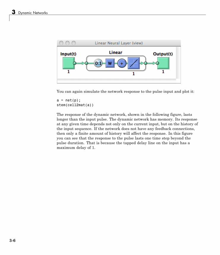
3 Dynamic Networks
You can again simulate the network response to the pulse input and plot it:
a = net(p);stem(cell2mat(a))
The response of the dynamic network, shown in the following figure, lastslonger than the input pulse. The dynamic network has memory. Its responseat any given time depends not only on the current input, but on the history ofthe input sequence. If the network does not have any feedback connections,then only a finite amount of history will affect the response. In this figureyou can see that the response to the pulse lasts one time step beyond thepulse duration. That is because the tapped delay line on the input has amaximum delay of 1.
3-6
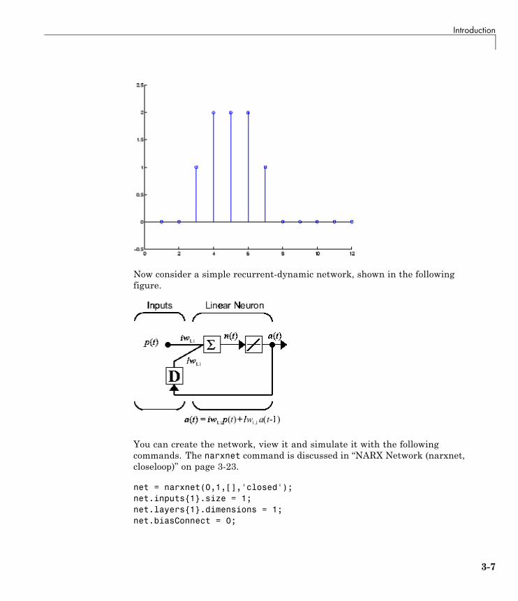
Introduction
Now consider a simple recurrent-dynamic network, shown in the followingfigure.
You can create the network, view it and simulate it with the followingcommands. The narxnet command is discussed in “NARX Network (narxnet,closeloop)” on page 3-23.
net = narxnet(0,1,[],'closed');net.inputs{1}.size = 1;net.layers{1}.dimensions = 1;net.biasConnect = 0;
3-7
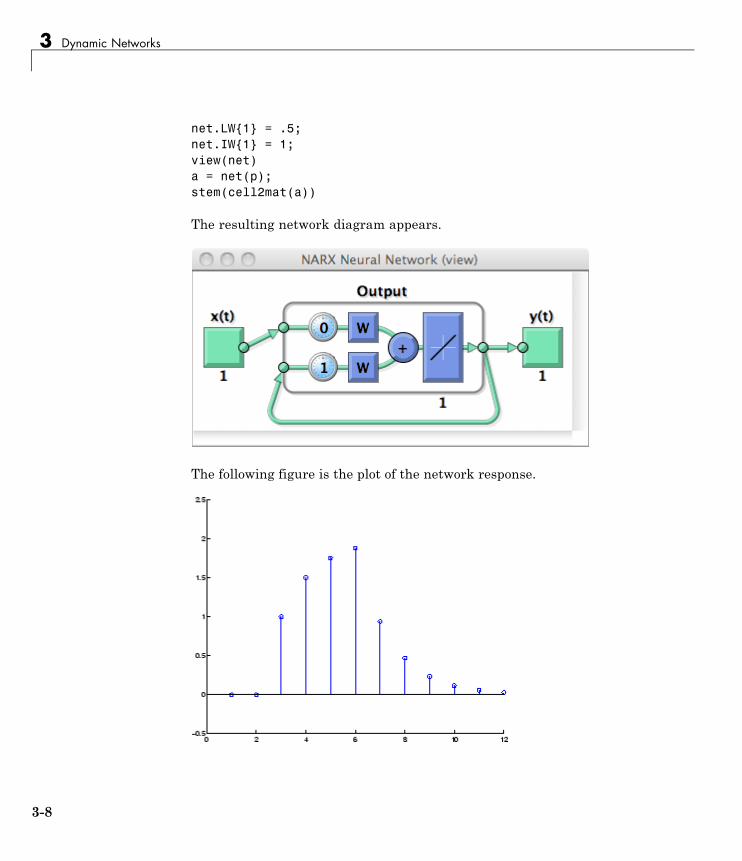
3 Dynamic Networks
net.LW{1} = .5;net.IW{1} = 1;view(net)a = net(p);stem(cell2mat(a))
The resulting network diagram appears.
The following figure is the plot of the network response.
3-8
Introduction
Notice that recurrent-dynamic networks typically have a longer response thanfeedforward-dynamic networks. For linear networks, feedforward-dynamicnetworks are called finite impulse response (FIR), because the response toan impulse input will become zero after a finite amount of time. Linearrecurrent-dynamic networks are called infinite impulse response (IIR),because the response to an impulse can decay to zero (for a stable network),but it will never become exactly equal to zero. An impulse response for anonlinear network cannot be defined, but the ideas of finite and infiniteresponses do carry over.
Applications of Dynamic NetworksDynamic networks are generally more powerful than static networks(although somewhat more difficult to train). Because dynamic networks havememory, they can be trained to learn sequential or time-varying patterns.This has applications in such disparate areas as prediction in financialmarkets [RoJa96], channel equalization in communication systems [FeTs03],phase detection in power systems [KaGr96], sorting [JaRa04], fault detection[ChDa99], speech recognition [Robin94], and even the prediction of proteinstructure in genetics [GiPr02]. You can find a discussion of many moredynamic network applications in [MeJa00].
One principal application of dynamic neural networks is in control systems.This application is discussed in detail in “Neural Network Control Systems”.Dynamic networks are also well suited for filtering. You will see the use ofsome linear dynamic networks for filtering in and some of those ideas areextended in this topic, using nonlinear dynamic networks.
Dynamic Network StructuresThe Neural Network Toolbox software is designed to train a class of networkcalled the Layered Digital Dynamic Network (LDDN). Any network that canbe arranged in the form of an LDDN can be trained with the toolbox. Hereis a basic description of the LDDN.
Each layer in the LDDN is made up of the following parts:
• Set of weight matrices that come into that layer (which can connect fromother layers or from external inputs), associated weight function rule used
3-9
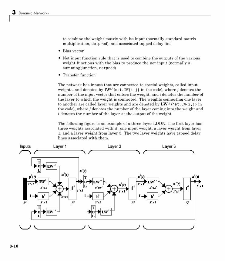
3 Dynamic Networks
to combine the weight matrix with its input (normally standard matrixmultiplication, dotprod), and associated tapped delay line
• Bias vector
• Net input function rule that is used to combine the outputs of the variousweight functions with the bias to produce the net input (normally asumming junction, netprod)
• Transfer function
The network has inputs that are connected to special weights, called inputweights, and denoted by IWi,j (net.IW{i,j} in the code), where j denotes thenumber of the input vector that enters the weight, and i denotes the number ofthe layer to which the weight is connected. The weights connecting one layerto another are called layer weights and are denoted by LWi,j (net.LW{i,j} inthe code), where j denotes the number of the layer coming into the weight andi denotes the number of the layer at the output of the weight.
The following figure is an example of a three-layer LDDN. The first layer hasthree weights associated with it: one input weight, a layer weight from layer1, and a layer weight from layer 3. The two layer weights have tapped delaylines associated with them.
3-10
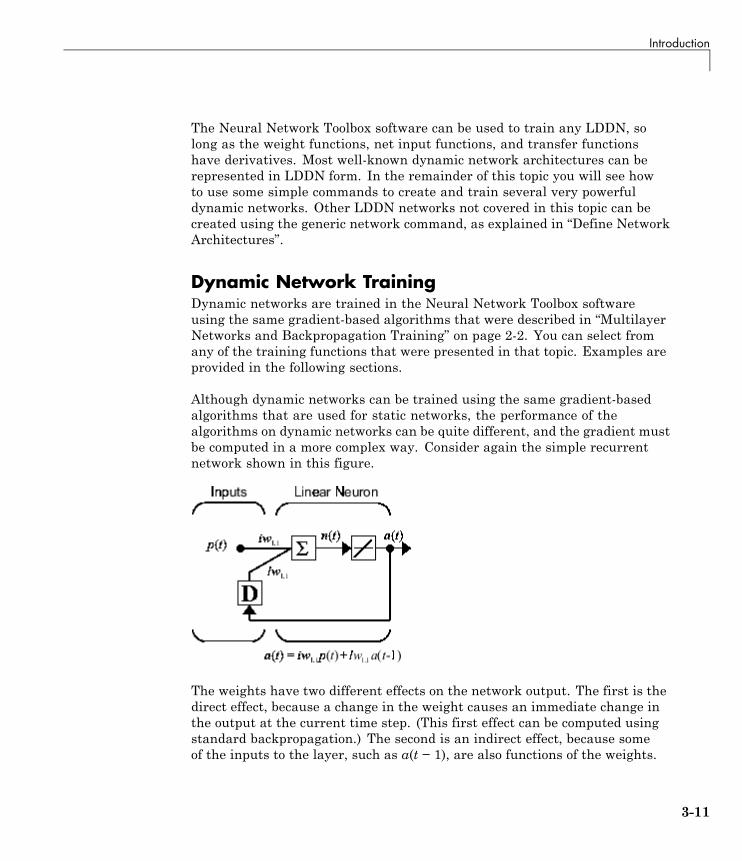
Introduction
The Neural Network Toolbox software can be used to train any LDDN, solong as the weight functions, net input functions, and transfer functionshave derivatives. Most well-known dynamic network architectures can berepresented in LDDN form. In the remainder of this topic you will see howto use some simple commands to create and train several very powerfuldynamic networks. Other LDDN networks not covered in this topic can becreated using the generic network command, as explained in “Define NetworkArchitectures”.
Dynamic Network TrainingDynamic networks are trained in the Neural Network Toolbox softwareusing the same gradient-based algorithms that were described in “MultilayerNetworks and Backpropagation Training” on page 2-2. You can select fromany of the training functions that were presented in that topic. Examples areprovided in the following sections.
Although dynamic networks can be trained using the same gradient-basedalgorithms that are used for static networks, the performance of thealgorithms on dynamic networks can be quite different, and the gradient mustbe computed in a more complex way. Consider again the simple recurrentnetwork shown in this figure.
The weights have two different effects on the network output. The first is thedirect effect, because a change in the weight causes an immediate change inthe output at the current time step. (This first effect can be computed usingstandard backpropagation.) The second is an indirect effect, because someof the inputs to the layer, such as a(t − 1), are also functions of the weights.
3-11
3 Dynamic Networks
To account for this indirect effect, you must use dynamic backpropagationto compute the gradients, which is more computationally intensive. (See[DeHa01a], [DeHa01b] and [DeHa07].) Expect dynamic backpropagation totake more time to train, in part for this reason. In addition, the error surfacesfor dynamic networks can be more complex than those for static networks.Training is more likely to be trapped in local minima. This suggests that youmight need to train the network several times to achieve an optimal result.See [DHH01] and [HDH09] for some discussion on the training of dynamicnetworks.
The remaining sections of this topic show how to create, train, and applycertain dynamic networks to modeling, detection, and forecasting problems.Some of the networks require dynamic backpropagation for computing thegradients and others do not. As a user, you do not need to decide whether ornot dynamic backpropagation is needed. This is determined automatically bythe software, which also decides on the best form of dynamic backpropagationto use. You just need to create the network and then invoke the standardtrain command.
3-12
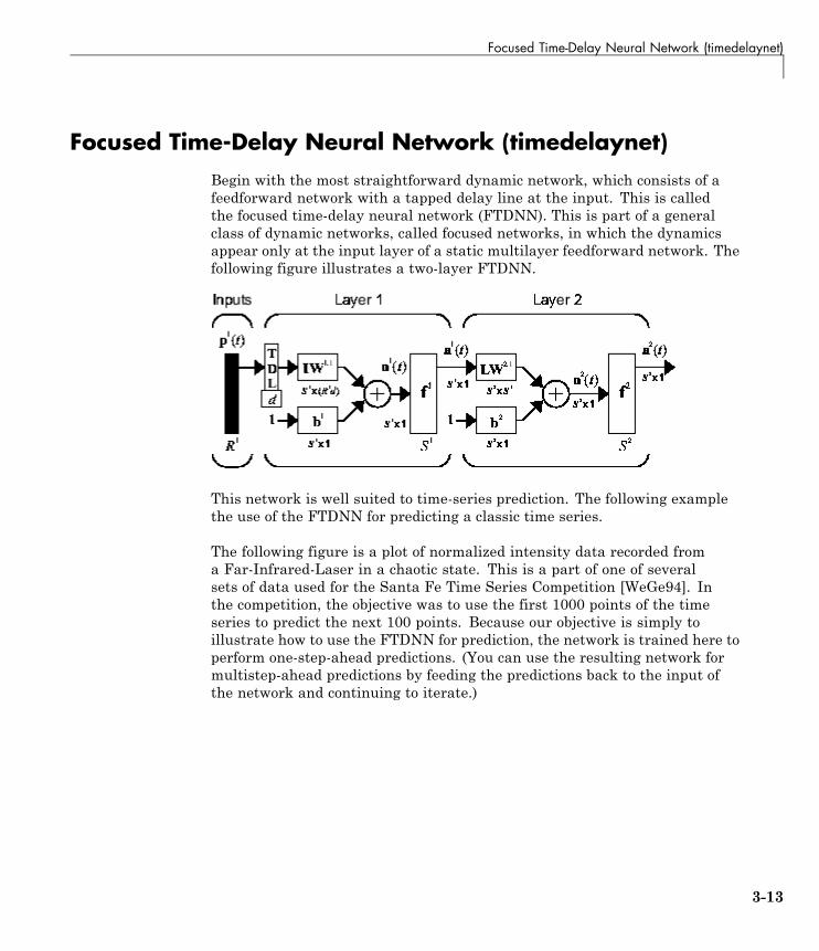
Focused Time-Delay Neural Network (timedelaynet)
Focused Time-Delay Neural Network (timedelaynet)Begin with the most straightforward dynamic network, which consists of afeedforward network with a tapped delay line at the input. This is calledthe focused time-delay neural network (FTDNN). This is part of a generalclass of dynamic networks, called focused networks, in which the dynamicsappear only at the input layer of a static multilayer feedforward network. Thefollowing figure illustrates a two-layer FTDNN.
This network is well suited to time-series prediction. The following examplethe use of the FTDNN for predicting a classic time series.
The following figure is a plot of normalized intensity data recorded froma Far-Infrared-Laser in a chaotic state. This is a part of one of severalsets of data used for the Santa Fe Time Series Competition [WeGe94]. Inthe competition, the objective was to use the first 1000 points of the timeseries to predict the next 100 points. Because our objective is simply toillustrate how to use the FTDNN for prediction, the network is trained here toperform one-step-ahead predictions. (You can use the resulting network formultistep-ahead predictions by feeding the predictions back to the input ofthe network and continuing to iterate.)
3-13
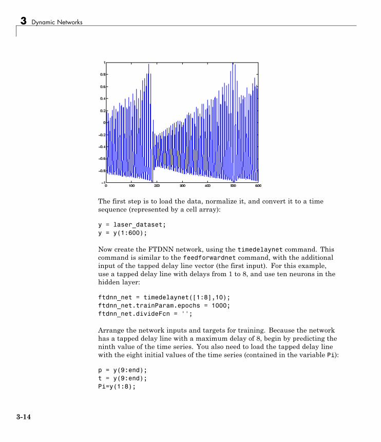
3 Dynamic Networks
The first step is to load the data, normalize it, and convert it to a timesequence (represented by a cell array):
y = laser_dataset;y = y(1:600);
Now create the FTDNN network, using the timedelaynet command. Thiscommand is similar to the feedforwardnet command, with the additionalinput of the tapped delay line vector (the first input). For this example,use a tapped delay line with delays from 1 to 8, and use ten neurons in thehidden layer:
ftdnn_net = timedelaynet([1:8],10);ftdnn_net.trainParam.epochs = 1000;ftdnn_net.divideFcn = '';
Arrange the network inputs and targets for training. Because the networkhas a tapped delay line with a maximum delay of 8, begin by predicting theninth value of the time series. You also need to load the tapped delay linewith the eight initial values of the time series (contained in the variable Pi):
p = y(9:end);t = y(9:end);Pi=y(1:8);
3-14
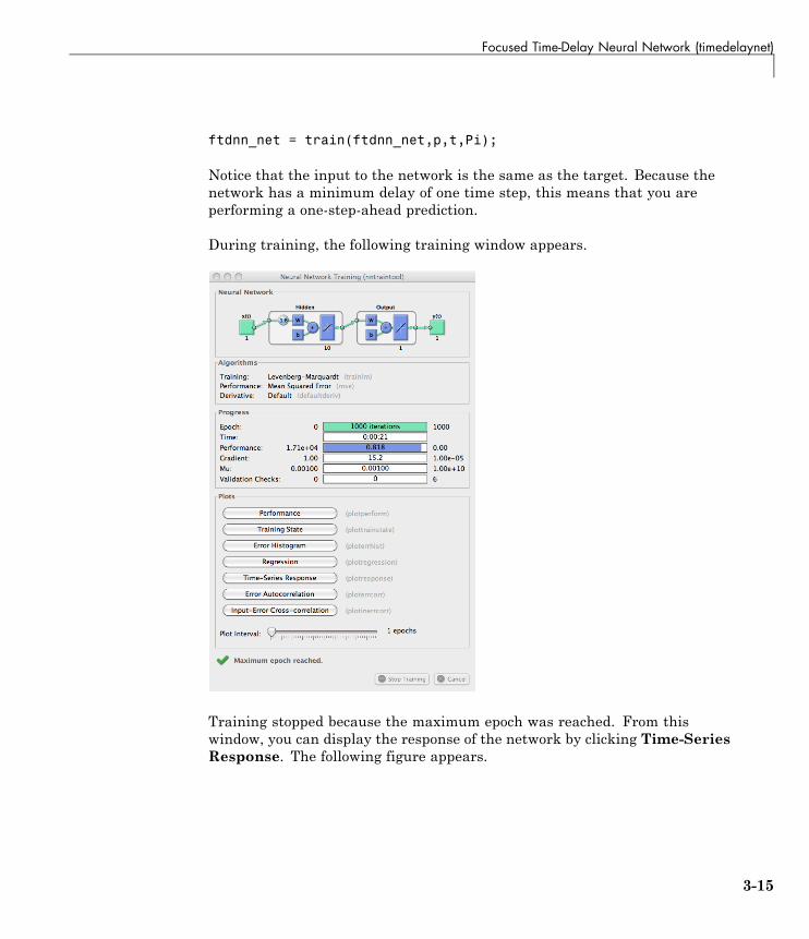
Focused Time-Delay Neural Network (timedelaynet)
ftdnn_net = train(ftdnn_net,p,t,Pi);
Notice that the input to the network is the same as the target. Because thenetwork has a minimum delay of one time step, this means that you areperforming a one-step-ahead prediction.
During training, the following training window appears.
Training stopped because the maximum epoch was reached. From thiswindow, you can display the response of the network by clicking Time-SeriesResponse. The following figure appears.
3-15
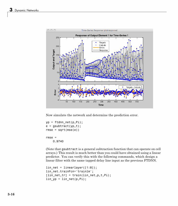
3 Dynamic Networks
Now simulate the network and determine the prediction error.
yp = ftdnn_net(p,Pi);e = gsubtract(yp,t);rmse = sqrt(mse(e))
rmse =0.9740
(Note that gsubtract is a general subtraction function that can operate on cellarrays.) This result is much better than you could have obtained using a linearpredictor. You can verify this with the following commands, which design alinear filter with the same tapped delay line input as the previous FTDNN.
lin_net = linearlayer([1:8]);lin_net.trainFcn='trainlm';[lin_net,tr] = train(lin_net,p,t,Pi);lin_yp = lin_net(p,Pi);
3-16
Focused Time-Delay Neural Network (timedelaynet)
lin_e = gsubtract(lin_yp,t);lin_rmse = sqrt(mse(lin_e))
lin_rmse =21.1386
The rms error is 21.1386 for the linear predictor, but 0.9740 for the nonlinearFTDNN predictor.
One nice feature of the FTDNN is that it does not require dynamicbackpropagation to compute the network gradient. This is because the tappeddelay line appears only at the input of the network, and contains no feedbackloops or adjustable parameters. For this reason, you will find that thisnetwork trains faster than other dynamic networks.
If you have an application for a dynamic network, try the linear network first(linearlayer) and then the FTDNN (timedelaynet). If neither networkis satisfactory, try one of the more complex dynamic networks discussed inthe remainder of this topic.
3-17
3 Dynamic Networks
Preparing Data (preparets)You will notice in the last section that for dynamic networks there is asignificant amount of data preparation that is required before training orsimulating the network. This is because the tapped delay lines in the networkneed to be filled with initial conditions, which requires that part of theoriginal data set be removed and shifted. (You can see the steps for doing this.) There is a toolbox function that facilitates the data preparation for dynamic(time series) networks - preparets. For example, the following lines:
p = y(9:end);t = y(9:end);Pi = y(1:8);
can be replaced with
[p,Pi,Ai,t] = preparets(ftdnn_net,y,y);
The preparets function uses the network object to determine how to fill thetapped delay lines with initial conditions, and how to shift the data to createthe correct inputs and targets to use in training or simulating the network.The general form for invoking preparets is
[X,Xi,Ai,T,EW,shift] = preparets(net,inputs,targets,feedback,EW)
The input arguments for preparets are the network object (net), theexternal (non-feedback) input to the network (inputs), the non-feedbacktarget (targets), the feedback target (feedback), and the error weights (EW)(see “Error Weighting” on page 3-40). The difference between external andfeedback signals will become clearer when the NARX network is described in“NARX Network (narxnet, closeloop)” on page 3-23. For the FTDNN network,there is no feedback signal.
The return arguments for preparets are the time shift between networkinputs and outputs (shift), the network input for training and simulation (X),the initial inputs (Xi) for loading the tapped delay lines for input weights, theinitial layer outputs (Ai) for loading the tapped delay lines for layer weights,the training targets (T), and the error weights (EW).
3-18

Preparing Data (preparets)
Using preparets eliminates the need to manually shift inputs and targets andload tapped delay lines. This is especially useful for more complex networks.
3-19
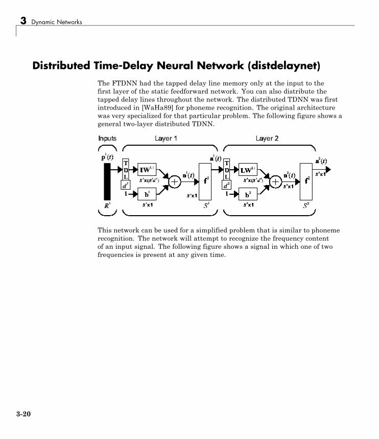
3 Dynamic Networks
Distributed Time-Delay Neural Network (distdelaynet)The FTDNN had the tapped delay line memory only at the input to thefirst layer of the static feedforward network. You can also distribute thetapped delay lines throughout the network. The distributed TDNN was firstintroduced in [WaHa89] for phoneme recognition. The original architecturewas very specialized for that particular problem. The following figure shows ageneral two-layer distributed TDNN.
This network can be used for a simplified problem that is similar to phonemerecognition. The network will attempt to recognize the frequency contentof an input signal. The following figure shows a signal in which one of twofrequencies is present at any given time.
3-20
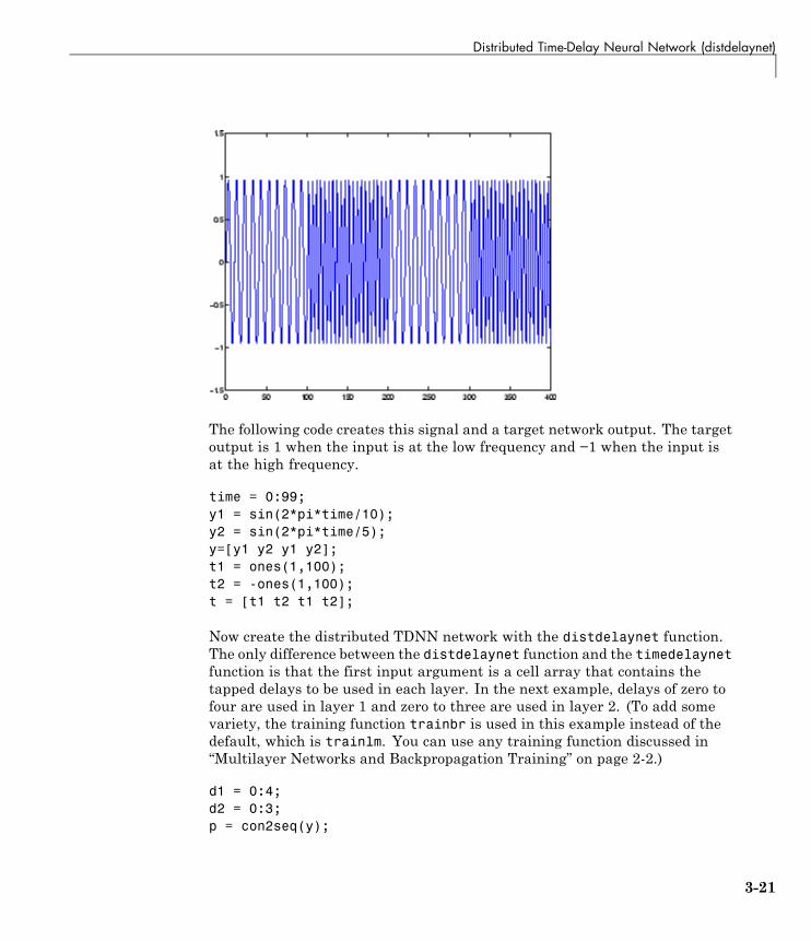
Distributed Time-Delay Neural Network (distdelaynet)
The following code creates this signal and a target network output. The targetoutput is 1 when the input is at the low frequency and −1 when the input isat the high frequency.
time = 0:99;y1 = sin(2*pi*time/10);y2 = sin(2*pi*time/5);y=[y1 y2 y1 y2];t1 = ones(1,100);t2 = -ones(1,100);t = [t1 t2 t1 t2];
Now create the distributed TDNN network with the distdelaynet function.The only difference between the distdelaynet function and the timedelaynetfunction is that the first input argument is a cell array that contains thetapped delays to be used in each layer. In the next example, delays of zero tofour are used in layer 1 and zero to three are used in layer 2. (To add somevariety, the training function trainbr is used in this example instead of thedefault, which is trainlm. You can use any training function discussed in“Multilayer Networks and Backpropagation Training” on page 2-2.)
d1 = 0:4;d2 = 0:3;p = con2seq(y);
3-21
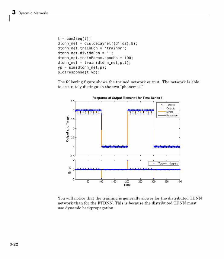
3 Dynamic Networks
t = con2seq(t);dtdnn_net = distdelaynet({d1,d2},5);dtdnn_net.trainFcn = 'trainbr';dtdnn_net.divideFcn = '';dtdnn_net.trainParam.epochs = 100;dtdnn_net = train(dtdnn_net,p,t);yp = sim(dtdnn_net,p);plotresponse(t,yp);
The following figure shows the trained network output. The network is ableto accurately distinguish the two “phonemes.”
You will notice that the training is generally slower for the distributed TDNNnetwork than for the FTDNN. This is because the distributed TDNN mustuse dynamic backpropagation.
3-22
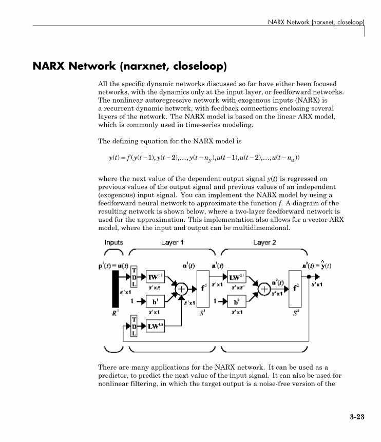
NARX Network (narxnet, closeloop)
NARX Network (narxnet, closeloop)All the specific dynamic networks discussed so far have either been focusednetworks, with the dynamics only at the input layer, or feedforward networks.The nonlinear autoregressive network with exogenous inputs (NARX) isa recurrent dynamic network, with feedback connections enclosing severallayers of the network. The NARX model is based on the linear ARX model,which is commonly used in time-series modeling.
The defining equation for the NARX model is
y t f y t y t y t n u t u t u t ny u( ) ( ( ), ( ), , ( ), ( ), ( ), , ( ))= − − − − − −1 2 1 2
where the next value of the dependent output signal y(t) is regressed onprevious values of the output signal and previous values of an independent(exogenous) input signal. You can implement the NARX model by using afeedforward neural network to approximate the function f. A diagram of theresulting network is shown below, where a two-layer feedforward network isused for the approximation. This implementation also allows for a vector ARXmodel, where the input and output can be multidimensional.
There are many applications for the NARX network. It can be used as apredictor, to predict the next value of the input signal. It can also be used fornonlinear filtering, in which the target output is a noise-free version of the
3-23
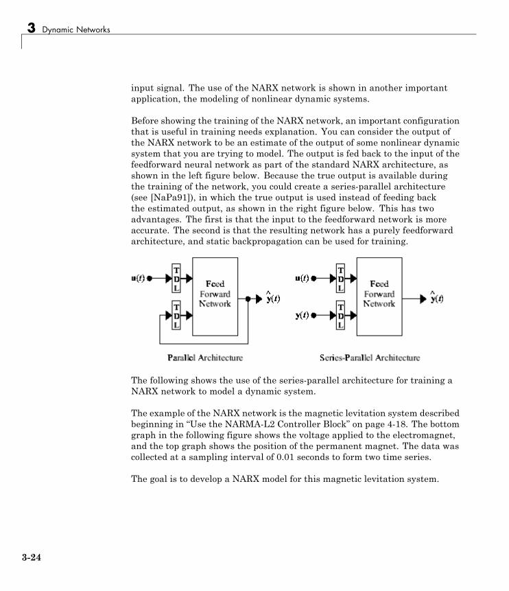
3 Dynamic Networks
input signal. The use of the NARX network is shown in another importantapplication, the modeling of nonlinear dynamic systems.
Before showing the training of the NARX network, an important configurationthat is useful in training needs explanation. You can consider the output ofthe NARX network to be an estimate of the output of some nonlinear dynamicsystem that you are trying to model. The output is fed back to the input of thefeedforward neural network as part of the standard NARX architecture, asshown in the left figure below. Because the true output is available duringthe training of the network, you could create a series-parallel architecture(see [NaPa91]), in which the true output is used instead of feeding backthe estimated output, as shown in the right figure below. This has twoadvantages. The first is that the input to the feedforward network is moreaccurate. The second is that the resulting network has a purely feedforwardarchitecture, and static backpropagation can be used for training.
The following shows the use of the series-parallel architecture for training aNARX network to model a dynamic system.
The example of the NARX network is the magnetic levitation system describedbeginning in “Use the NARMA-L2 Controller Block” on page 4-18. The bottomgraph in the following figure shows the voltage applied to the electromagnet,and the top graph shows the position of the permanent magnet. The data wascollected at a sampling interval of 0.01 seconds to form two time series.
The goal is to develop a NARX model for this magnetic levitation system.
3-24
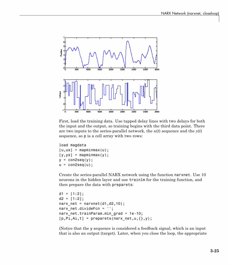
NARX Network (narxnet, closeloop)
First, load the training data. Use tapped delay lines with two delays for boththe input and the output, so training begins with the third data point. Thereare two inputs to the series-parallel network, the u(t) sequence and the y(t)sequence, so p is a cell array with two rows:
load magdata[u,us] = mapminmax(u);[y,ys] = mapminmax(y);y = con2seq(y);u = con2seq(u);
Create the series-parallel NARX network using the function narxnet. Use 10neurons in the hidden layer and use trainlm for the training function, andthen prepare the data with preparets:
d1 = [1:2];d2 = [1:2];narx_net = narxnet(d1,d2,10);narx_net.divideFcn = '';narx_net.trainParam.min_grad = 1e-10;[p,Pi,Ai,t] = preparets(narx_net,u,{},y);
(Notice that the y sequence is considered a feedback signal, which is an inputthat is also an output (target). Later, when you close the loop, the appropriate
3-25
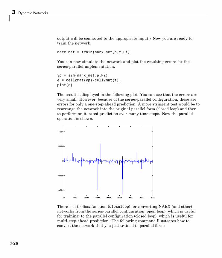
3 Dynamic Networks
output will be connected to the appropriate input.) Now you are ready totrain the network.
narx_net = train(narx_net,p,t,Pi);
You can now simulate the network and plot the resulting errors for theseries-parallel implementation.
yp = sim(narx_net,p,Pi);e = cell2mat(yp)-cell2mat(t);plot(e)
The result is displayed in the following plot. You can see that the errors arevery small. However, because of the series-parallel configuration, these areerrors for only a one-step-ahead prediction. A more stringent test would be torearrange the network into the original parallel form (closed loop) and thento perform an iterated prediction over many time steps. Now the paralleloperation is shown.
There is a toolbox function (closeloop) for converting NARX (and other)networks from the series-parallel configuration (open loop), which is usefulfor training, to the parallel configuration (closed loop), which is useful formulti-step-ahead prediction. The following command illustrates how toconvert the network that you just trained to parallel form:
3-26
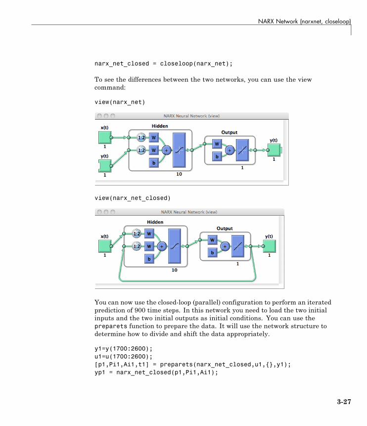
NARX Network (narxnet, closeloop)
narx_net_closed = closeloop(narx_net);
To see the differences between the two networks, you can use the viewcommand:
view(narx_net)
view(narx_net_closed)
You can now use the closed-loop (parallel) configuration to perform an iteratedprediction of 900 time steps. In this network you need to load the two initialinputs and the two initial outputs as initial conditions. You can use thepreparets function to prepare the data. It will use the network structure todetermine how to divide and shift the data appropriately.
y1=y(1700:2600);u1=u(1700:2600);[p1,Pi1,Ai1,t1] = preparets(narx_net_closed,u1,{},y1);yp1 = narx_net_closed(p1,Pi1,Ai1);
3-27
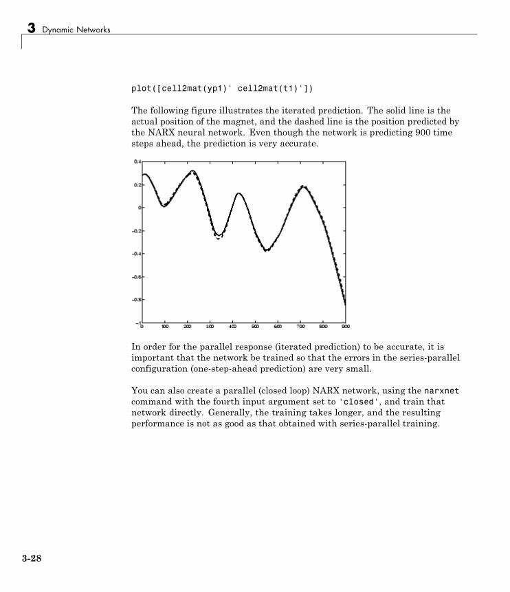
3 Dynamic Networks
plot([cell2mat(yp1)' cell2mat(t1)'])
The following figure illustrates the iterated prediction. The solid line is theactual position of the magnet, and the dashed line is the position predicted bythe NARX neural network. Even though the network is predicting 900 timesteps ahead, the prediction is very accurate.
In order for the parallel response (iterated prediction) to be accurate, it isimportant that the network be trained so that the errors in the series-parallelconfiguration (one-step-ahead prediction) are very small.
You can also create a parallel (closed loop) NARX network, using the narxnetcommand with the fourth input argument set to 'closed', and train thatnetwork directly. Generally, the training takes longer, and the resultingperformance is not as good as that obtained with series-parallel training.
3-28
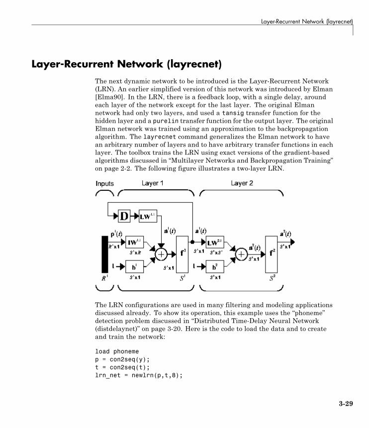
Layer-Recurrent Network (layrecnet)
Layer-Recurrent Network (layrecnet)The next dynamic network to be introduced is the Layer-Recurrent Network(LRN). An earlier simplified version of this network was introduced by Elman[Elma90]. In the LRN, there is a feedback loop, with a single delay, aroundeach layer of the network except for the last layer. The original Elmannetwork had only two layers, and used a tansig transfer function for thehidden layer and a purelin transfer function for the output layer. The originalElman network was trained using an approximation to the backpropagationalgorithm. The layrecnet command generalizes the Elman network to havean arbitrary number of layers and to have arbitrary transfer functions in eachlayer. The toolbox trains the LRN using exact versions of the gradient-basedalgorithms discussed in “Multilayer Networks and Backpropagation Training”on page 2-2. The following figure illustrates a two-layer LRN.
The LRN configurations are used in many filtering and modeling applicationsdiscussed already. To show its operation, this example uses the “phoneme”detection problem discussed in “Distributed Time-Delay Neural Network(distdelaynet)” on page 3-20. Here is the code to load the data and to createand train the network:
load phonemep = con2seq(y);t = con2seq(t);lrn_net = newlrn(p,t,8);
3-29
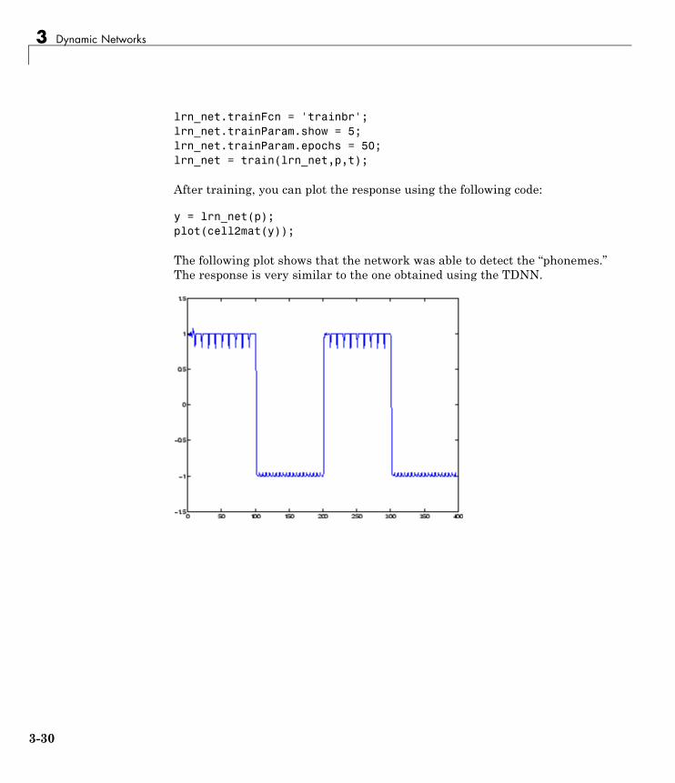
3 Dynamic Networks
lrn_net.trainFcn = 'trainbr';lrn_net.trainParam.show = 5;lrn_net.trainParam.epochs = 50;lrn_net = train(lrn_net,p,t);
After training, you can plot the response using the following code:
y = lrn_net(p);plot(cell2mat(y));
The following plot shows that the network was able to detect the “phonemes.”The response is very similar to the one obtained using the TDNN.
3-30
Training Custom Networks
Training Custom NetworksSo far, this topic has described the training procedures for several specificdynamic network architectures. However, any network that can be createdin the toolbox can be trained using the training functions described in“Multilayer Networks and Backpropagation Training” on page 2-2 so longas the components of the network are differentiable. This section givesan example of how to create and train a custom architecture. The customarchitecture you will use is the model reference adaptive control (MRAC)system that is described in detail in “Model Reference Control” on page 4-23.
As you can see in “Model Reference Control” on page 4-23, the model referencecontrol architecture has two subnetworks. One subnetwork is the model ofthe plant that you want to control. The other subnetwork is the controller.You will begin by training a NARX network that will become the plant modelsubnetwork. For this example, you will use the robot arm to represent theplant, as described in “Model Reference Control” on page 4-23. The followingcode will load data collected from the robot arm and create and train a NARXnetwork. For this simple problem, you do not need to preprocess the data, andall of the data can be used for training, so no data division is needed.
[u,y] = robotarm_dataset;d1 = [1:2];d2 = [1:2];S1 = 5;narx_net = narxnet(d1,d2,S1);narx_net.divideFcn = '';narx_net.inputs{1}.processFcns = {};narx_net.inputs{2}.processFcns = {};narx_net.outputs{2}.processFcns = {};narx_net.trainParam.min_grad = 1e-10;[p,Pi,Ai,t] = preparets(narx_net,u,{},y);narx_net = train(narx_net,p,t,Pi);narx_net_closed = closeloop(narx_net);view(narx_net_closed)
The resulting network is shown in the following figure.
3-31
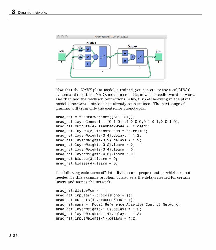
3 Dynamic Networks
Now that the NARX plant model is trained, you can create the total MRACsystem and insert the NARX model inside. Begin with a feedforward network,and then add the feedback connections. Also, turn off learning in the plantmodel subnetwork, since it has already been trained. The next stage oftraining will train only the controller subnetwork.
mrac_net = feedforwardnet([S1 1 S1]);mrac_net.layerConnect = [0 1 0 1;1 0 0 0;0 1 0 1;0 0 1 0];mrac_net.outputs{4}.feedbackMode = 'closed';mrac_net.layers{2}.transferFcn = 'purelin';mrac_net.layerWeights{3,4}.delays = 1:2;mrac_net.layerWeights{3,2}.delays = 1:2;mrac_net.layerWeights{3,2}.learn = 0;mrac_net.layerWeights{3,4}.learn = 0;mrac_net.layerWeights{4,3}.learn = 0;mrac_net.biases{3}.learn = 0;mrac_net.biases{4}.learn = 0;
The following code turns off data division and preprocessing, which are notneeded for this example problem. It also sets the delays needed for certainlayers and names the network.
mrac_net.divideFcn = '';mrac_net.inputs{1}.processFcns = {};mrac_net.outputs{4}.processFcns = {};mrac_net.name = 'Model Reference Adaptive Control Network';mrac_net.layerWeights{1,2}.delays = 1:2;mrac_net.layerWeights{1,4}.delays = 1:2;mrac_net.inputWeights{1}.delays = 1:2;
3-32
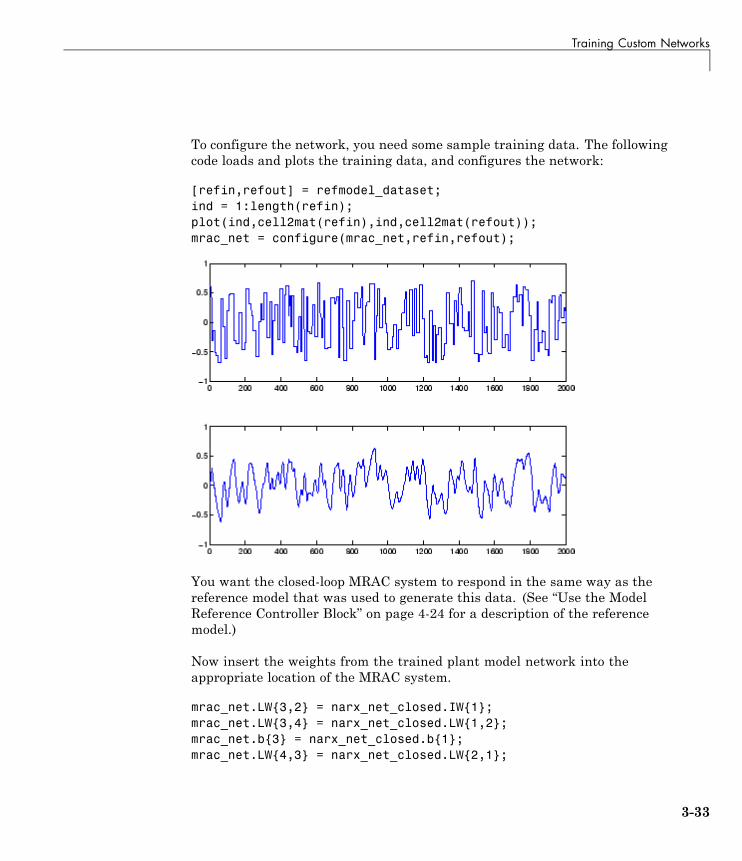
Training Custom Networks
To configure the network, you need some sample training data. The followingcode loads and plots the training data, and configures the network:
[refin,refout] = refmodel_dataset;ind = 1:length(refin);plot(ind,cell2mat(refin),ind,cell2mat(refout));mrac_net = configure(mrac_net,refin,refout);
You want the closed-loop MRAC system to respond in the same way as thereference model that was used to generate this data. (See “Use the ModelReference Controller Block” on page 4-24 for a description of the referencemodel.)
Now insert the weights from the trained plant model network into theappropriate location of the MRAC system.
mrac_net.LW{3,2} = narx_net_closed.IW{1};mrac_net.LW{3,4} = narx_net_closed.LW{1,2};mrac_net.b{3} = narx_net_closed.b{1};mrac_net.LW{4,3} = narx_net_closed.LW{2,1};
3-33
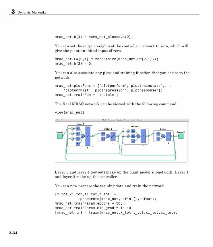
3 Dynamic Networks
mrac_net.b{4} = narx_net_closed.b{2};
You can set the output weights of the controller network to zero, which willgive the plant an initial input of zero.
mrac_net.LW{2,1} = zeros(size(mrac_net.LW{2,1}));mrac_net.b{2} = 0;
You can also associate any plots and training function that you desire to thenetwork.
mrac_net.plotFcns = {'plotperform','plottrainstate',...'ploterrhist','plotregression','plotresponse'};
mrac_net.trainFcn = 'trainlm';
The final MRAC network can be viewed with the following command:
view(mrac_net)
Layer 3 and layer 4 (output) make up the plant model subnetwork. Layer 1and layer 2 make up the controller.
You can now prepare the training data and train the network.
[x_tot,xi_tot,ai_tot,t_tot] = ...preparets(mrac_net,refin,{},refout);
mrac_net.trainParam.epochs = 50;mrac_net.trainParam.min_grad = 1e-10;[mrac_net,tr] = train(mrac_net,x_tot,t_tot,xi_tot,ai_tot);
3-34
Training Custom Networks
Note Notice that you are using the trainlm training function here, butany of the training functions discussed in “Multilayer Networks andBackpropagation Training” on page 2-2 could be used as well. Any networkthat you can create in the toolbox can be trained with any of those trainingfunctions. The only limitation is that all of the parts of the network mustbe differentiable.
You will find that the training of the MRAC system takes much longerthat the training of the NARX plant model. This is because the network isrecurrent and dynamic backpropagation must be used. This is determinedautomatically by the toolbox software and does not require any userintervention. There are several implementations of dynamic backpropagation(see [DeHa07]), and the toolbox software automatically determines the mostefficient one for the selected network architecture and training algorithm.
After the network has been trained, you can test the operation by applying atest input to the MRAC network. The following code creates a skyline inputfunction, which is a series of steps of random height and width, and applies itto the trained MRAC network.
testin = skyline(1000,50,200,-.7,.7);testinseq = con2seq(testin);testoutseq = mrac_net(testinseq);testout = cell2mat(testoutseq);figure;plot([testin' testout'])
From the figure below, you can see that the plant model output does followthe reference input with the correct critically damped response, even thoughthe input sequence was not the same as the input sequence in the trainingdata. The steady state response is not perfect for each step, but this could beimproved with a larger training set and perhaps more hidden neurons.
The purpose of this example was to show that you can create your own customdynamic network and train it using the standard toolbox training functionswithout any modifications. Any network that you can create in the toolbox canbe trained with the standard training functions, as long as each component ofthe network has a defined derivative.
3-35
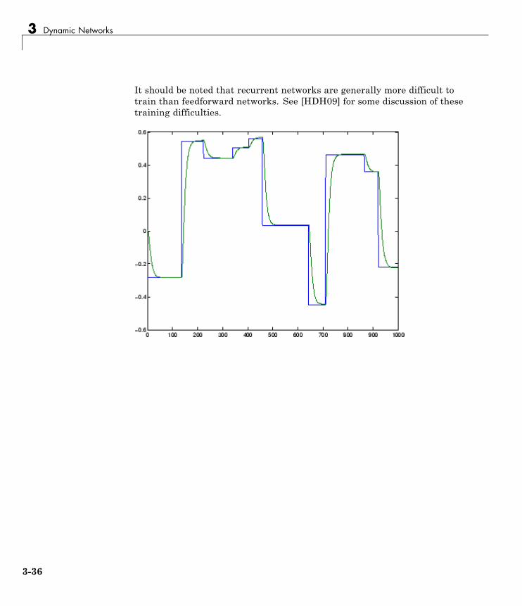
3 Dynamic Networks
It should be noted that recurrent networks are generally more difficult totrain than feedforward networks. See [HDH09] for some discussion of thesetraining difficulties.
3-36
Multiple Sequences, Time-Series Utilities, and Error Weighting
Multiple Sequences, Time-Series Utilities, and ErrorWeighting
There are a number of utility functions available in the toolbox formanipulating time series data sets. This section describes some of thesefunctions, as well as a technique for weighting errors.
Multiple SequencesThere are times when time-series data is not available in one long sequence,but rather as several shorter sequences. When dealing with static networksand concurrent batches of static data, you can simply append data setstogether to form one large concurrent batch. However, you would notgenerally want to append time sequences together, since that would cause adiscontinuity in the sequence. For these cases, you can create a concurrent setof sequences, as described in “Data Structures” on page 1-24.
When training a network with a concurrent set of sequences, it is requiredthat each sequence be of the same length. If this is not the case, then theshorter sequence inputs and targets should be padded with NaNs, in order tomake all sequences the same length. The targets that are assigned values ofNaN will be ignored during the calculation of network performance.
The following code illustrates the use of the function catsamples to combineseveral sequences together to form a concurrent set of sequences, while at thesame time padding the shorter sequences.
load magmulseqy_mul = catsamples(y1,y2,y3,'pad');u_mul = catsamples(u1,u2,u3,'pad');d1 = [1:2];d2 = [1:2];narx_net = narxnet(d1,d2,10);narx_net.divideFcn = '';narx_net.trainParam.min_grad = 1e-10;[p,Pi,Ai,t] = preparets(narx_net,u_mul,{},y_mul);narx_net = train(narx_net,p,t,Pi);
3-37
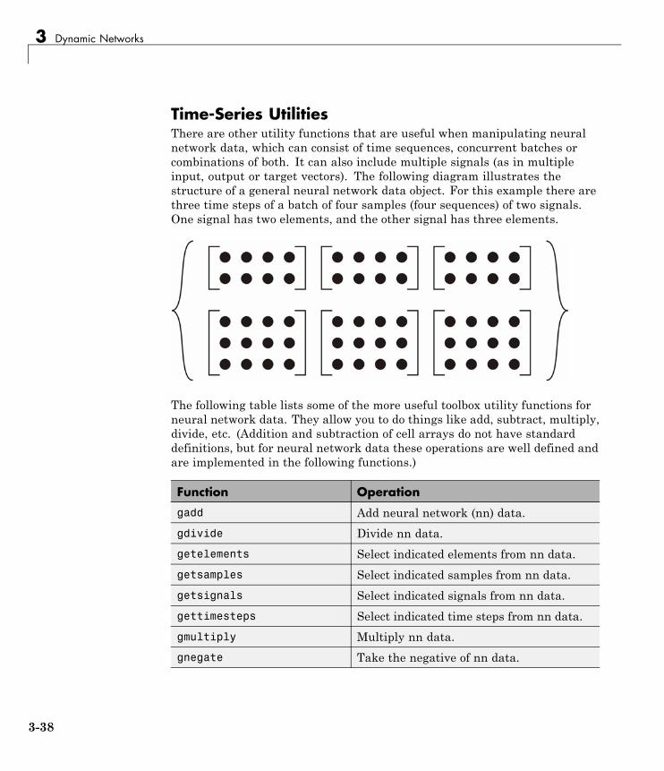
3 Dynamic Networks
Time-Series UtilitiesThere are other utility functions that are useful when manipulating neuralnetwork data, which can consist of time sequences, concurrent batches orcombinations of both. It can also include multiple signals (as in multipleinput, output or target vectors). The following diagram illustrates thestructure of a general neural network data object. For this example there arethree time steps of a batch of four samples (four sequences) of two signals.One signal has two elements, and the other signal has three elements.
The following table lists some of the more useful toolbox utility functions forneural network data. They allow you to do things like add, subtract, multiply,divide, etc. (Addition and subtraction of cell arrays do not have standarddefinitions, but for neural network data these operations are well defined andare implemented in the following functions.)
Function Operation
gadd Add neural network (nn) data.
gdivide Divide nn data.
getelements Select indicated elements from nn data.
getsamples Select indicated samples from nn data.
getsignals Select indicated signals from nn data.
gettimesteps Select indicated time steps from nn data.
gmultiply Multiply nn data.
gnegate Take the negative of nn data.
3-38

Multiple Sequences, Time-Series Utilities, and Error Weighting
Function Operation
gsubtract Subtract nn data.
nndata Create an nn data object of specified size,where values are assigned randomly or toa constant.
nnsize Return number of elements, samples, timesteps and signals in an nn data object.
numelements Return the number of elements in nn data.
numsamples Return the number of samples in nn data.
numsignals Return the number of signals in nn data.
numtimesteps Return the number of time steps in nndata.
setelements Set specified elements of nn data.
setsamples Set specified samples of nn data.
setsignals Set specified signals of nn data.
settimesteps Set specified time steps of nn data.
There are also some useful plotting and analysis functions for dynamicnetworks that are listed in the following table. There are examples of usingthese functions in the “Getting Started with Neural Network Toolbox”.
Function Operation
ploterrcorr Plot the autocorrelation function of theerror.
plotinerrcorr Plot the crosscorrelation between the errorand the input.
plotresponse Plot network output and target versustime.
3-39
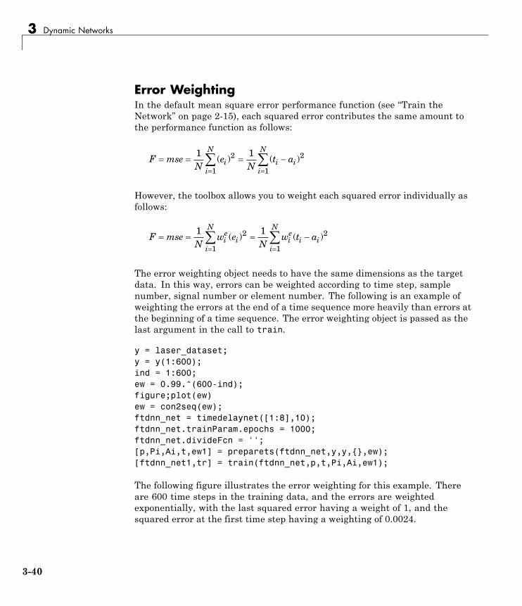
3 Dynamic Networks
Error WeightingIn the default mean square error performance function (see “Train theNetwork” on page 2-15), each squared error contributes the same amount tothe performance function as follows:
F mseN
eN
t aii
N
i ii
N
1 12
1
2
1( ) ( )
However, the toolbox allows you to weight each squared error individually asfollows:
F mseN
w eN
w t aie
ii
N
ie
i ii
N
1 12
1
2
1( ) ( )
The error weighting object needs to have the same dimensions as the targetdata. In this way, errors can be weighted according to time step, samplenumber, signal number or element number. The following is an example ofweighting the errors at the end of a time sequence more heavily than errors atthe beginning of a time sequence. The error weighting object is passed as thelast argument in the call to train.
y = laser_dataset;y = y(1:600);ind = 1:600;ew = 0.99.^(600-ind);figure;plot(ew)ew = con2seq(ew);ftdnn_net = timedelaynet([1:8],10);ftdnn_net.trainParam.epochs = 1000;ftdnn_net.divideFcn = '';[p,Pi,Ai,t,ew1] = preparets(ftdnn_net,y,y,{},ew);[ftdnn_net1,tr] = train(ftdnn_net,p,t,Pi,Ai,ew1);
The following figure illustrates the error weighting for this example. Thereare 600 time steps in the training data, and the errors are weightedexponentially, with the last squared error having a weight of 1, and thesquared error at the first time step having a weighting of 0.0024.
3-40
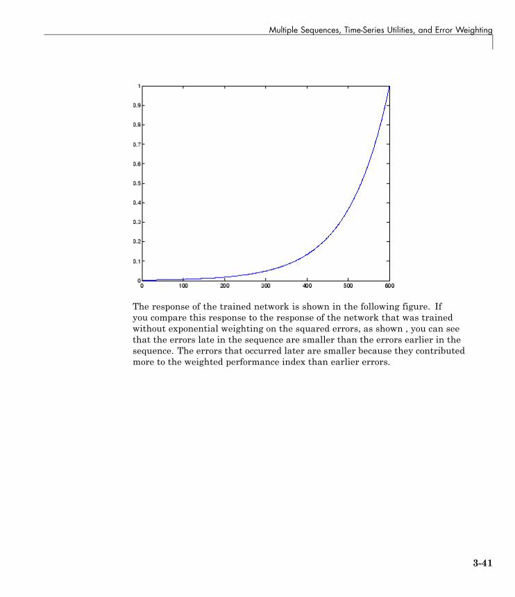
Multiple Sequences, Time-Series Utilities, and Error Weighting
The response of the trained network is shown in the following figure. Ifyou compare this response to the response of the network that was trainedwithout exponential weighting on the squared errors, as shown , you can seethat the errors late in the sequence are smaller than the errors earlier in thesequence. The errors that occurred later are smaller because they contributedmore to the weighted performance index than earlier errors.
3-41
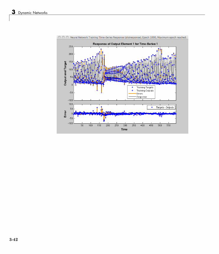
3 Dynamic Networks
3-42

4
Control Systems
• “Introduction to System Control” on page 4-2
• “NN Predictive Control” on page 4-4
• “NARMA-L2 (Feedback Linearization) Control” on page 4-14
• “Model Reference Control” on page 4-23
• “Import and Export” on page 4-31
4 Control Systems
Introduction to System ControlNeural networks have been applied successfully in the identification andcontrol of dynamic systems. The universal approximation capabilities of themultilayer perceptron make it a popular choice for modeling nonlinear systemsand for implementing general-purpose nonlinear controllers [HaDe99]. Thischapter introduces three popular neural network architectures for predictionand control that have been implemented in the Neural Network Toolboxsoftware:
• Model Predictive Control
• NARMA-L2 (or Feedback Linearization) Control
• Model Reference Control
This chapter presents brief descriptions of each of these architectures andshows how you can use them.
There are typically two steps involved when using neural networks for control:
1 System identification
2 Control design
In the system identification stage, you develop a neural network model ofthe plant that you want to control. In the control design stage, you use theneural network plant model to design (or train) the controller. In each of thethree control architectures described in this chapter, the system identificationstage is identical. The control design stage, however, is different for eacharchitecture:
• For model predictive control, the plant model is used to predict futurebehavior of the plant, and an optimization algorithm is used to select thecontrol input that optimizes future performance.
• For NARMA-L2 control, the controller is simply a rearrangement of theplant model.
• For model reference control, the controller is a neural network that istrained to control a plant so that it follows a reference model. The neuralnetwork plant model is used to assist in the controller training.
4-2
Introduction to System Control
The next three sections of this chapter discuss model predictive control,NARMA-L2 control, and model reference control. Each section consists of abrief description of the control concept, followed by an example of the use ofthe appropriate Neural Network Toolbox function. These three controllersare implemented as Simulink® blocks, which are contained in the NeuralNetwork Toolbox blockset.
To assist you in determining the best controller for your application, thefollowing list summarizes the key controller features. Each controller has itsown strengths and weaknesses. No single controller is appropriate for everyapplication.
• Model Predictive Control — This controller uses a neural networkmodel to predict future plant responses to potential control signals. Anoptimization algorithm then computes the control signals that optimizefuture plant performance. The neural network plant model is trainedoffline, in batch form. (This is true for all three control architectures.) Thecontroller, however, requires a significant amount of online computation,because an optimization algorithm is performed at each sample time tocompute the optimal control input.
• NARMA-L2 Control— This controller requires the least computation ofthese three architectures. The controller is simply a rearrangement of theneural network plant model, which is trained offline, in batch form. Theonly online computation is a forward pass through the neural networkcontroller. The drawback of this method is that the plant must either bein companion form, or be capable of approximation by a companion formmodel. (“Identification of the NARMA-L2 Model” on page 4-14 describesthe companion form model.)
• Model Reference Control— The online computation of this controller,like NARMA-L2, is minimal. However, unlike NARMA-L2, the modelreference architecture requires that a separate neural network controllerbe trained offline, in addition to the neural network plant model. Thecontroller training is computationally expensive, because it requires theuse of dynamic backpropagation [HaJe99]. On the positive side, modelreference control applies to a larger class of plant than does NARMA-L2control.
4-3
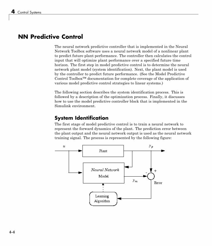
4 Control Systems
NN Predictive ControlThe neural network predictive controller that is implemented in the NeuralNetwork Toolbox software uses a neural network model of a nonlinear plantto predict future plant performance. The controller then calculates the controlinput that will optimize plant performance over a specified future timehorizon. The first step in model predictive control is to determine the neuralnetwork plant model (system identification). Next, the plant model is usedby the controller to predict future performance. (See the Model PredictiveControl Toolbox™ documentation for complete coverage of the application ofvarious model predictive control strategies to linear systems.)
The following section describes the system identification process. This isfollowed by a description of the optimization process. Finally, it discusseshow to use the model predictive controller block that is implemented in theSimulink environment.
System IdentificationThe first stage of model predictive control is to train a neural network torepresent the forward dynamics of the plant. The prediction error betweenthe plant output and the neural network output is used as the neural networktraining signal. The process is represented by the following figure:
4-4
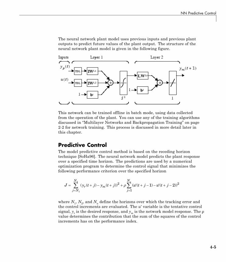
NN Predictive Control
The neural network plant model uses previous inputs and previous plantoutputs to predict future values of the plant output. The structure of theneural network plant model is given in the following figure.
This network can be trained offline in batch mode, using data collectedfrom the operation of the plant. You can use any of the training algorithmsdiscussed in “Multilayer Networks and Backpropagation Training” on page2-2 for network training. This process is discussed in more detail later inthis chapter.
Predictive ControlThe model predictive control method is based on the receding horizontechnique [SoHa96]. The neural network model predicts the plant responseover a specified time horizon. The predictions are used by a numericaloptimization program to determine the control signal that minimizes thefollowing performance criterion over the specified horizon
J y t j y t j u t j u t jr mj
N
j N
N u
( ( ) ( )) ( ( ) ( ))2 2
11 2
1
2
where N1, N2, and Nu define the horizons over which the tracking error andthe control increments are evaluated. The u′ variable is the tentative controlsignal, yr is the desired response, and ym is the network model response. The ρvalue determines the contribution that the sum of the squares of the controlincrements has on the performance index.
4-5
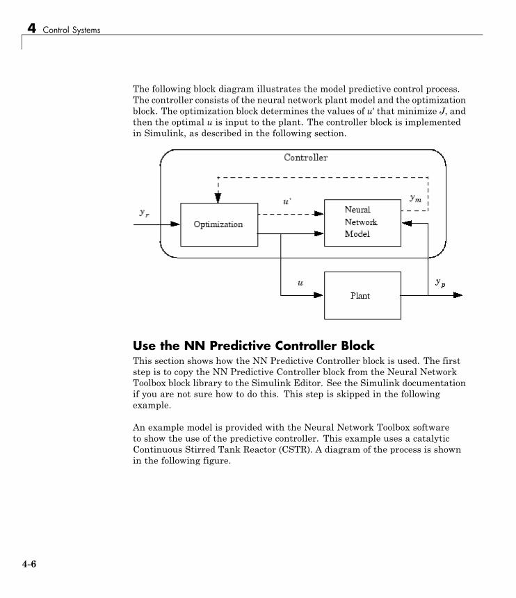
4 Control Systems
The following block diagram illustrates the model predictive control process.The controller consists of the neural network plant model and the optimizationblock. The optimization block determines the values of u′ that minimize J, andthen the optimal u is input to the plant. The controller block is implementedin Simulink, as described in the following section.
Use the NN Predictive Controller BlockThis section shows how the NN Predictive Controller block is used. The firststep is to copy the NN Predictive Controller block from the Neural NetworkToolbox block library to the Simulink Editor. See the Simulink documentationif you are not sure how to do this. This step is skipped in the followingexample.
An example model is provided with the Neural Network Toolbox softwareto show the use of the predictive controller. This example uses a catalyticContinuous Stirred Tank Reactor (CSTR). A diagram of the process is shownin the following figure.
4-6
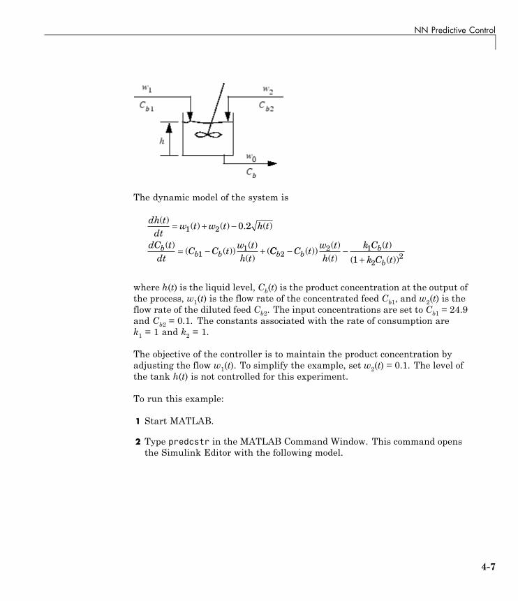
NN Predictive Control
The dynamic model of the system is
dh tdt
w t w t h t
dC tdt
C C tw th t
bb b
( )( ) ( ) . ( )
( )( ( ))
( )( )
(
= + −
= − +
1 2
11
0 2
CC C tw th t
k C t
k C tb b
b
b2
2 1
221
− −+
( ))( )
( )( )
( ( ))
where h(t) is the liquid level, Cb(t) is the product concentration at the output ofthe process, w1(t) is the flow rate of the concentrated feed Cb1, and w2(t) is theflow rate of the diluted feed Cb2. The input concentrations are set to Cb1 = 24.9and Cb2 = 0.1. The constants associated with the rate of consumption arek1 = 1 and k2 = 1.
The objective of the controller is to maintain the product concentration byadjusting the flow w1(t). To simplify the example, set w2(t) = 0.1. The level ofthe tank h(t) is not controlled for this experiment.
To run this example:
1 Start MATLAB.
2 Type predcstr in the MATLAB Command Window. This command opensthe Simulink Editor with the following model.
4-7
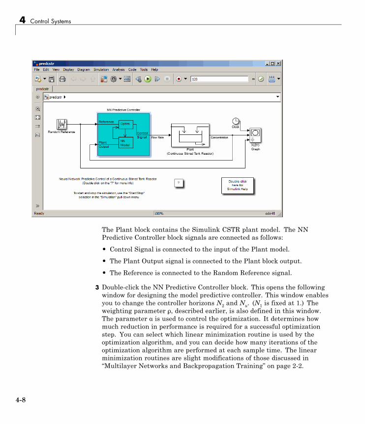
4 Control Systems
The Plant block contains the Simulink CSTR plant model. The NNPredictive Controller block signals are connected as follows:
• Control Signal is connected to the input of the Plant model.
• The Plant Output signal is connected to the Plant block output.
• The Reference is connected to the Random Reference signal.
3 Double-click the NN Predictive Controller block. This opens the followingwindow for designing the model predictive controller. This window enablesyou to change the controller horizons N2 and Nu. (N1 is fixed at 1.) Theweighting parameter ρ, described earlier, is also defined in this window.The parameter α is used to control the optimization. It determines howmuch reduction in performance is required for a successful optimizationstep. You can select which linear minimization routine is used by theoptimization algorithm, and you can decide how many iterations of theoptimization algorithm are performed at each sample time. The linearminimization routines are slight modifications of those discussed in“Multilayer Networks and Backpropagation Training” on page 2-2.
4-8
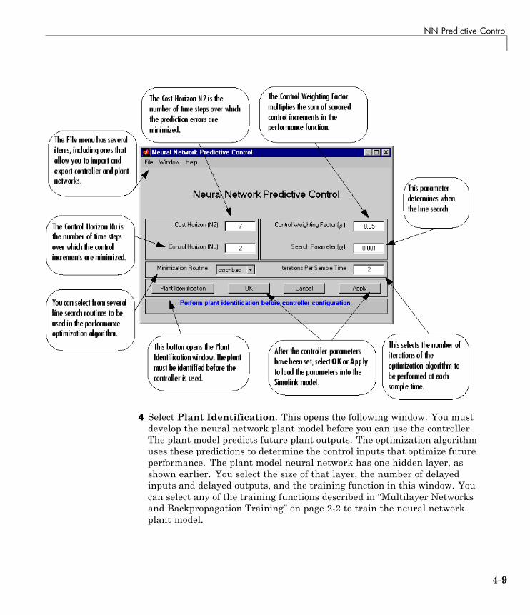
NN Predictive Control
4 Select Plant Identification. This opens the following window. You mustdevelop the neural network plant model before you can use the controller.The plant model predicts future plant outputs. The optimization algorithmuses these predictions to determine the control inputs that optimize futureperformance. The plant model neural network has one hidden layer, asshown earlier. You select the size of that layer, the number of delayedinputs and delayed outputs, and the training function in this window. Youcan select any of the training functions described in “Multilayer Networksand Backpropagation Training” on page 2-2 to train the neural networkplant model.
4-9
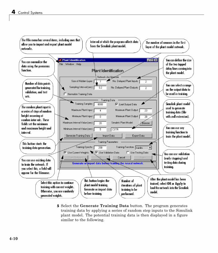
4 Control Systems
5 Select the Generate Training Data button. The program generatestraining data by applying a series of random step inputs to the Simulinkplant model. The potential training data is then displayed in a figuresimilar to the following.
4-10
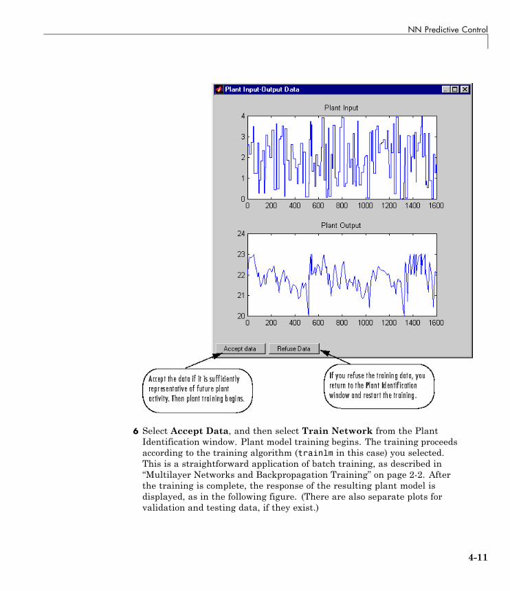
NN Predictive Control
6 Select Accept Data, and then select Train Network from the PlantIdentification window. Plant model training begins. The training proceedsaccording to the training algorithm (trainlm in this case) you selected.This is a straightforward application of batch training, as described in“Multilayer Networks and Backpropagation Training” on page 2-2. Afterthe training is complete, the response of the resulting plant model isdisplayed, as in the following figure. (There are also separate plots forvalidation and testing data, if they exist.)
4-11
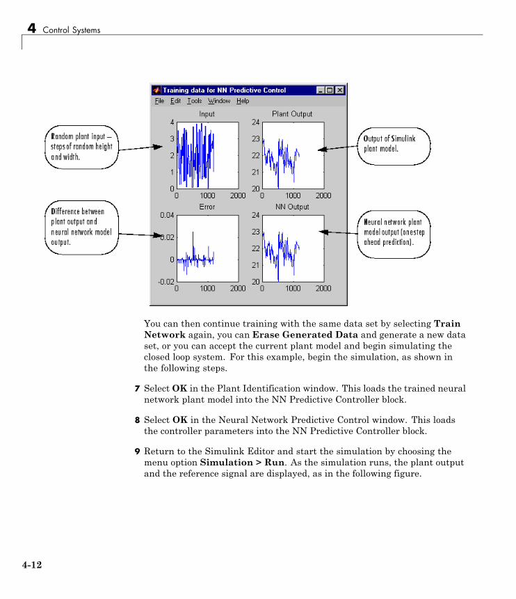
4 Control Systems
You can then continue training with the same data set by selecting TrainNetwork again, you can Erase Generated Data and generate a new dataset, or you can accept the current plant model and begin simulating theclosed loop system. For this example, begin the simulation, as shown inthe following steps.
7 Select OK in the Plant Identification window. This loads the trained neuralnetwork plant model into the NN Predictive Controller block.
8 Select OK in the Neural Network Predictive Control window. This loadsthe controller parameters into the NN Predictive Controller block.
9 Return to the Simulink Editor and start the simulation by choosing themenu option Simulation > Run. As the simulation runs, the plant outputand the reference signal are displayed, as in the following figure.
4-12
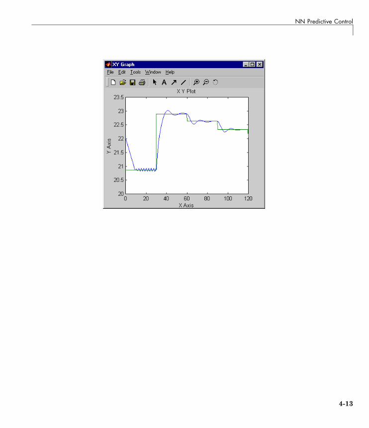
NN Predictive Control
4-13
4 Control Systems
NARMA-L2 (Feedback Linearization) ControlThe neurocontroller described in this section is referred to by two differentnames: feedback linearization control and NARMA-L2 control. It is referredto as feedback linearization when the plant model has a particular form(companion form). It is referred to as NARMA-L2 control when the plantmodel can be approximated by the same form. The central idea of this type ofcontrol is to transform nonlinear system dynamics into linear dynamics bycanceling the nonlinearities. This section begins by presenting the companionform system model and showing how you can use a neural network to identifythis model. Then it describes how the identified neural network model canbe used to develop a controller. This is followed by an example of how to usethe NARMA-L2 Control block, which is contained in the Neural NetworkToolbox blockset.
Identification of the NARMA-L2 ModelAs with model predictive control, the first step in using feedback linearization(or NARMA-L2) control is to identify the system to be controlled. You traina neural network to represent the forward dynamics of the system. Thefirst step is to choose a model structure to use. One standard model that isused to represent general discrete-time nonlinear systems is the nonlinearautoregressive-moving average (NARMA) model:
y k d N y k y k y k n u k u k u k n( ) [ ( ), ( ), , ( ), ( ), ( ), , ( )]+ = − − + − − +1 1 1 1
where u(k) is the system input, and y(k) is the system output. For theidentification phase, you could train a neural network to approximate thenonlinear function N. This is the identification procedure used for the NNPredictive Controller.
If you want the system output to follow some reference trajectoryy(k + d) = yr(k + d), the next step is to develop a nonlinear controller of theform:
u k G y k y k y k n y k d u k u k mr( ) [ ( ), ( ), , ( ), ( ), ( ), , ( )]= − − + + − − +1 1 1 1
The problem with using this controller is that if you want to train a neuralnetwork to create the function G to minimize mean square error, you need
4-14
NARMA-L2 (Feedback Linearization) Control
to use dynamic backpropagation ([NaPa91] or [HaJe99]). This can be quiteslow. One solution, proposed by Narendra and Mukhopadhyay [NaMu97], isto use approximate models to represent the system. The controller used inthis section is based on the NARMA-L2 approximate model:
ˆ( ) [ ( ), ( ), , ( ), ( ), , ( )][ ( )
y k d f y k y k y k n u k u k mg y k
1 1 1 1
,, ( ), , ( ), ( ), , ( )] ( )y k y k n u k u k m u k 1 1 1 1
This model is in companion form, where the next controller input u(k) is notcontained inside the nonlinearity. The advantage of this form is that youcan solve for the control input that causes the system output to follow thereference y(k + d) = yr(k + d). The resulting controller would have the form
u ky k d f y k y k y k n u k u k n
gr( )( ) [ ( ), ( ), , ( ), ( ), , ( )]
[= + − − − + − − +1 1 1 1
yy k y k y k n u k u k n( ), ( ), , ( ), ( ), , ( )]− − + − − +1 1 1 1
Using this equation directly can cause realization problems, because youmust determine the control input u(k) based on the output at the same time,y(k). So, instead, use the model
y k d f y k y k y k n u k u k u k ng
( ) [ ( ), ( ), , ( ), ( ), ( ), , ( )][
1 1 1 1
yy k y k n u k u k n u k( ), , ( ), ( ), , ( )] ( ) 1 1 1
where d ≥ 2. The following figure shows the structure of a neural networkrepresentation.
4-15
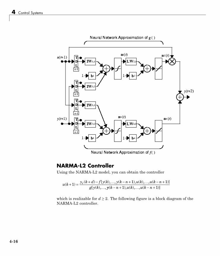
4 Control Systems
NARMA-L2 ControllerUsing the NARMA-L2 model, you can obtain the controller
u ky k d f y k y k n u k u k n
g y kr( )( ) [ ( ), , ( ), ( ), , ( )]
[ ( ), ,+ = + − − + − +
11 1
yy k n u k u k n( ), ( ), , ( )]− + − +1 1
which is realizable for d ≥ 2. The following figure is a block diagram of theNARMA-L2 controller.
4-16
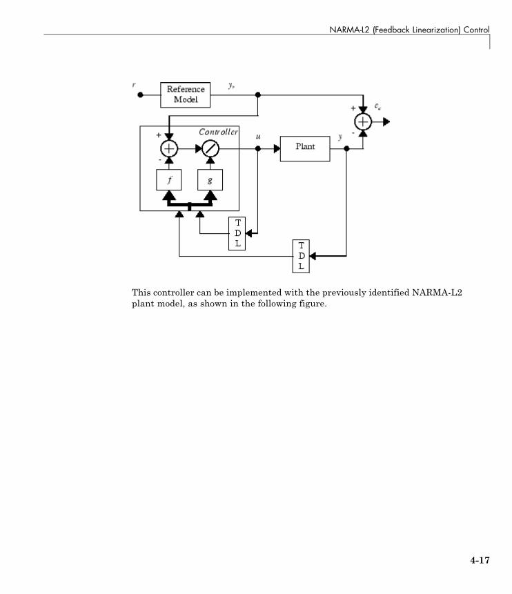
NARMA-L2 (Feedback Linearization) Control
This controller can be implemented with the previously identified NARMA-L2plant model, as shown in the following figure.
4-17
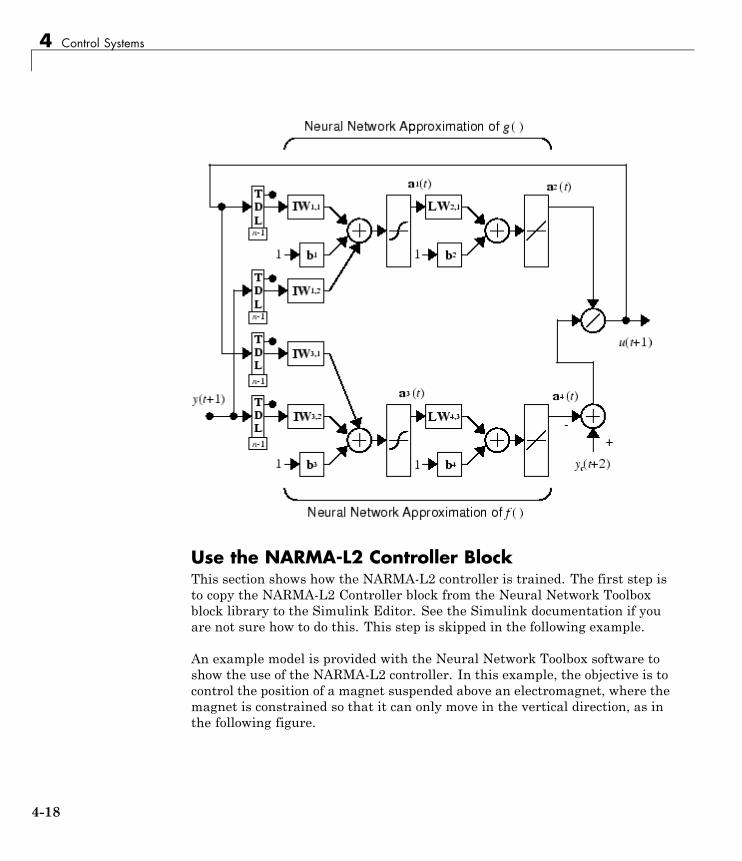
4 Control Systems
Use the NARMA-L2 Controller BlockThis section shows how the NARMA-L2 controller is trained. The first step isto copy the NARMA-L2 Controller block from the Neural Network Toolboxblock library to the Simulink Editor. See the Simulink documentation if youare not sure how to do this. This step is skipped in the following example.
An example model is provided with the Neural Network Toolbox software toshow the use of the NARMA-L2 controller. In this example, the objective is tocontrol the position of a magnet suspended above an electromagnet, where themagnet is constrained so that it can only move in the vertical direction, as inthe following figure.
4-18
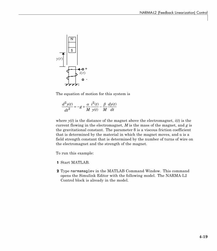
NARMA-L2 (Feedback Linearization) Control
The equation of motion for this system is
d y t
dtg
Mi ty t M
dy tdt
2
2
2( ) ( )( )
( )= − + −
where y(t) is the distance of the magnet above the electromagnet, i(t) is thecurrent flowing in the electromagnet, M is the mass of the magnet, and g isthe gravitational constant. The parameter β is a viscous friction coefficientthat is determined by the material in which the magnet moves, and α is afield strength constant that is determined by the number of turns of wire onthe electromagnet and the strength of the magnet.
To run this example:
1 Start MATLAB.
2 Type narmamaglev in the MATLAB Command Window. This commandopens the Simulink Editor with the following model. The NARMA-L2Control block is already in the model.
4-19
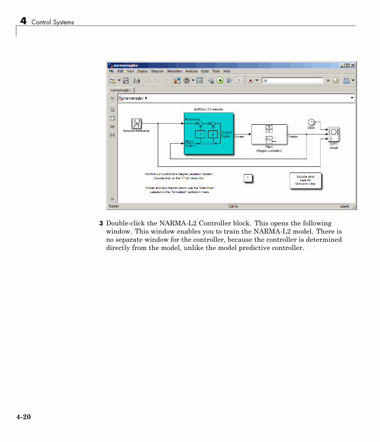
4 Control Systems
3 Double-click the NARMA-L2 Controller block. This opens the followingwindow. This window enables you to train the NARMA-L2 model. There isno separate window for the controller, because the controller is determineddirectly from the model, unlike the model predictive controller.
4-20
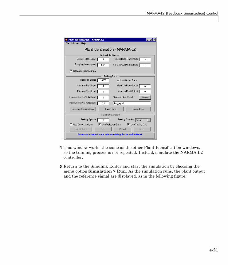
NARMA-L2 (Feedback Linearization) Control
4 This window works the same as the other Plant Identification windows,so the training process is not repeated. Instead, simulate the NARMA-L2controller.
5 Return to the Simulink Editor and start the simulation by choosing themenu option Simulation > Run. As the simulation runs, the plant outputand the reference signal are displayed, as in the following figure.
4-21
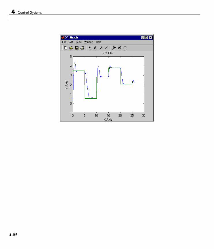
4 Control Systems
4-22
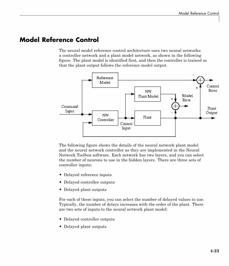
Model Reference Control
Model Reference ControlThe neural model reference control architecture uses two neural networks:a controller network and a plant model network, as shown in the followingfigure. The plant model is identified first, and then the controller is trained sothat the plant output follows the reference model output.
The following figure shows the details of the neural network plant modeland the neural network controller as they are implemented in the NeuralNetwork Toolbox software. Each network has two layers, and you can selectthe number of neurons to use in the hidden layers. There are three sets ofcontroller inputs:
• Delayed reference inputs
• Delayed controller outputs
• Delayed plant outputs
For each of these inputs, you can select the number of delayed values to use.Typically, the number of delays increases with the order of the plant. Thereare two sets of inputs to the neural network plant model:
• Delayed controller outputs
• Delayed plant outputs
4-23
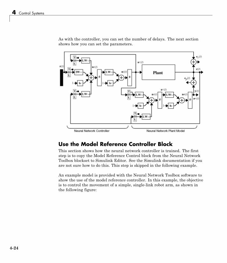
4 Control Systems
As with the controller, you can set the number of delays. The next sectionshows how you can set the parameters.
Use the Model Reference Controller BlockThis section shows how the neural network controller is trained. The firststep is to copy the Model Reference Control block from the Neural NetworkToolbox blockset to Simulink Editor. See the Simulink documentation if youare not sure how to do this. This step is skipped in the following example.
An example model is provided with the Neural Network Toolbox software toshow the use of the model reference controller. In this example, the objectiveis to control the movement of a simple, single-link robot arm, as shown inthe following figure:
4-24
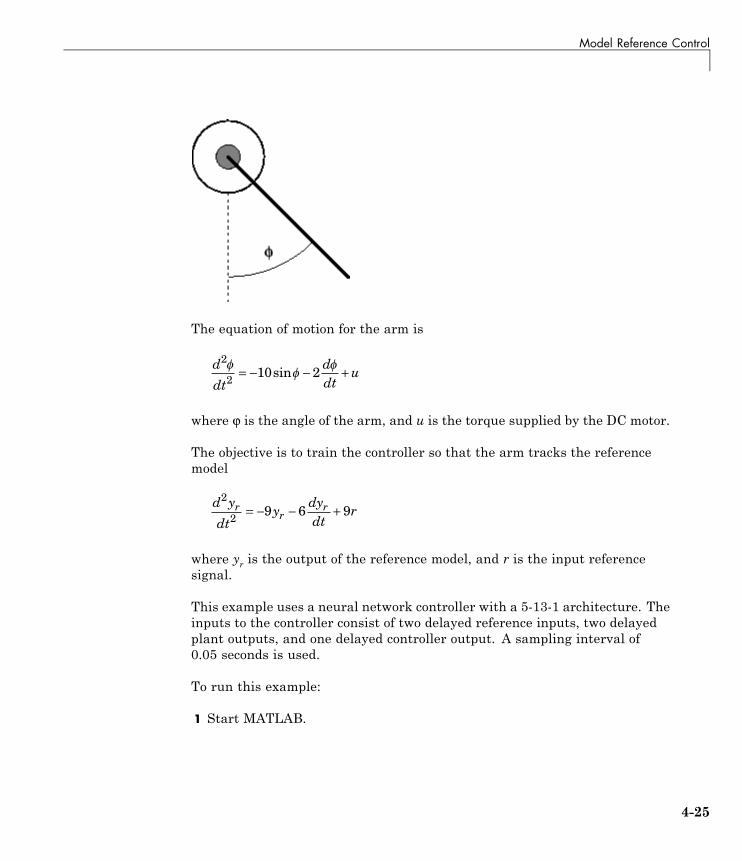
Model Reference Control
The equation of motion for the arm is
d
dt
ddt
u2
210 2
= − − +sin
where ϕ is the angle of the arm, and u is the torque supplied by the DC motor.
The objective is to train the controller so that the arm tracks the referencemodel
d y
dty
dydt
rrr
r2
29 6 9= − − +
where yr is the output of the reference model, and r is the input referencesignal.
This example uses a neural network controller with a 5-13-1 architecture. Theinputs to the controller consist of two delayed reference inputs, two delayedplant outputs, and one delayed controller output. A sampling interval of0.05 seconds is used.
To run this example:
1 Start MATLAB.
4-25
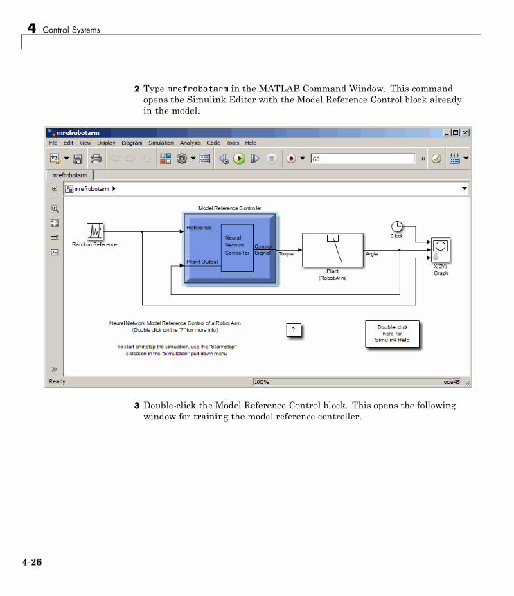
4 Control Systems
2 Type mrefrobotarm in the MATLAB Command Window. This commandopens the Simulink Editor with the Model Reference Control block alreadyin the model.
3 Double-click the Model Reference Control block. This opens the followingwindow for training the model reference controller.
4-26
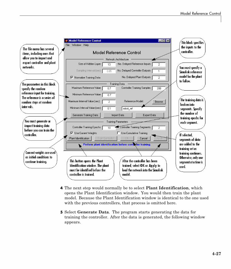
Model Reference Control
4 The next step would normally be to select Plant Identification, whichopens the Plant Identification window. You would then train the plantmodel. Because the Plant Identification window is identical to the one usedwith the previous controllers, that process is omitted here.
5 Select Generate Data. The program starts generating the data fortraining the controller. After the data is generated, the following windowappears.
4-27
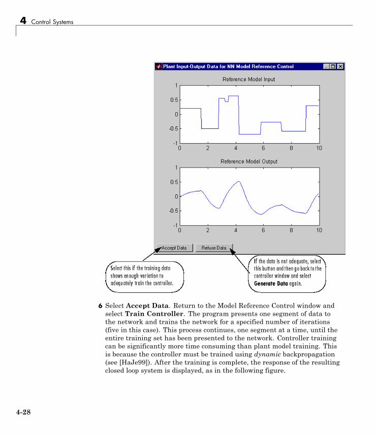
4 Control Systems
6 Select Accept Data. Return to the Model Reference Control window andselect Train Controller. The program presents one segment of data tothe network and trains the network for a specified number of iterations(five in this case). This process continues, one segment at a time, until theentire training set has been presented to the network. Controller trainingcan be significantly more time consuming than plant model training. Thisis because the controller must be trained using dynamic backpropagation(see [HaJe99]). After the training is complete, the response of the resultingclosed loop system is displayed, as in the following figure.
4-28
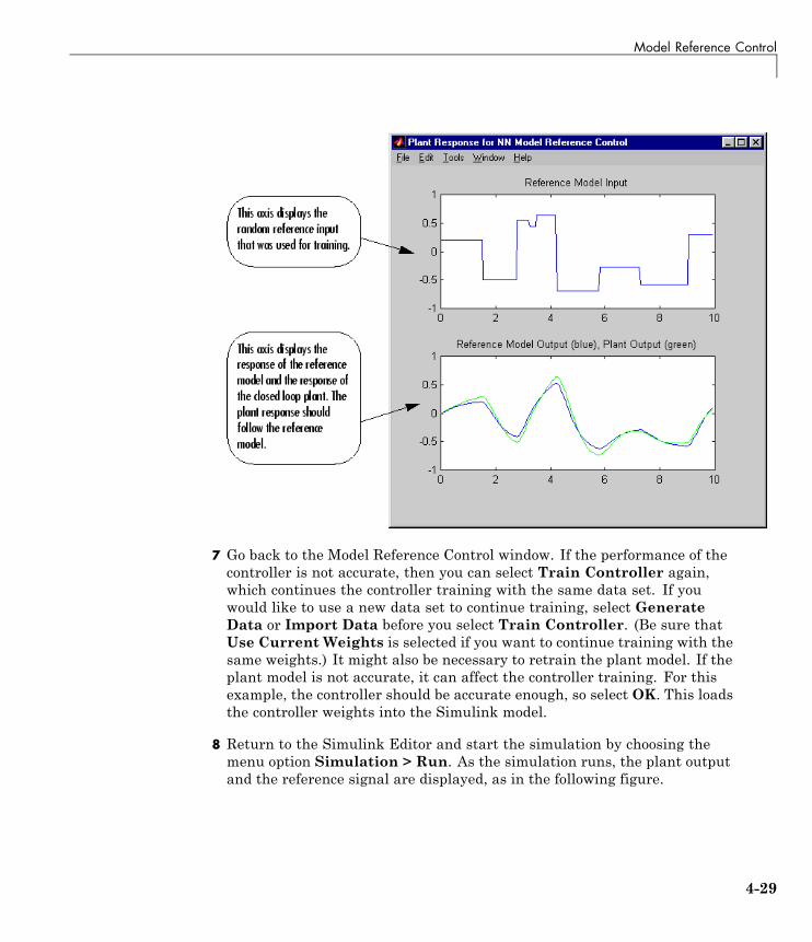
Model Reference Control
7 Go back to the Model Reference Control window. If the performance of thecontroller is not accurate, then you can select Train Controller again,which continues the controller training with the same data set. If youwould like to use a new data set to continue training, select GenerateData or Import Data before you select Train Controller. (Be sure thatUse Current Weights is selected if you want to continue training with thesame weights.) It might also be necessary to retrain the plant model. If theplant model is not accurate, it can affect the controller training. For thisexample, the controller should be accurate enough, so select OK. This loadsthe controller weights into the Simulink model.
8 Return to the Simulink Editor and start the simulation by choosing themenu option Simulation > Run. As the simulation runs, the plant outputand the reference signal are displayed, as in the following figure.
4-29
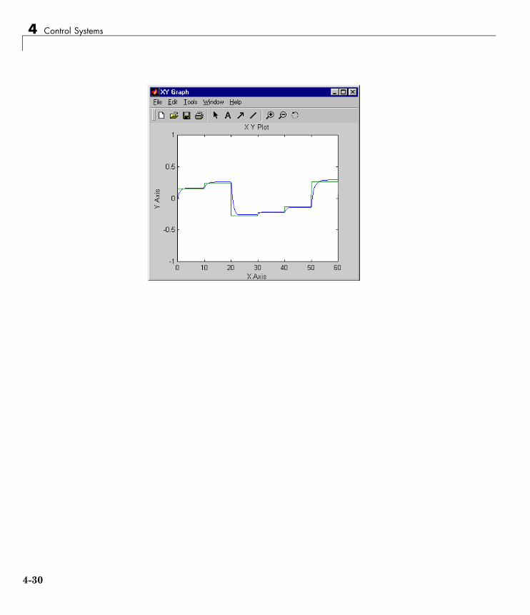
4 Control Systems
4-30

Import and Export
Import and Export
Import and Export NetworksThe controller and plant model networks that you develop are stored withinSimulink controller blocks. At some point you might want to transfer thenetworks into other applications, or you might want to transfer a networkfrom one controller block to another. You can do this by using the ImportNetwork and Export Network menu options. The following example leadsyou through the export and import processes. (The NARMA-L2 window isused for this example, but the same procedure applies to all the controllers.)
1 Repeat the first three steps of the NARMA-L2 example in “Use theNARMA-L2 Controller Block” on page 4-18. The NARMA-L2 PlantIdentification window should now be open.
2 Select File > Export Network, as shown below.
This opens the following window.
4-31
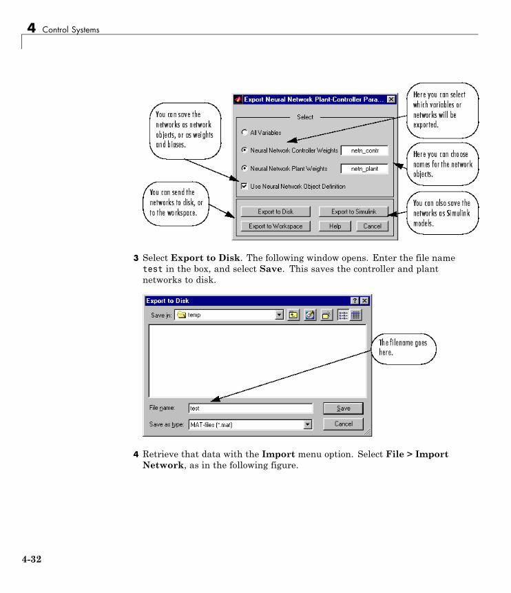
4 Control Systems
3 Select Export to Disk. The following window opens. Enter the file nametest in the box, and select Save. This saves the controller and plantnetworks to disk.
4 Retrieve that data with the Import menu option. Select File > ImportNetwork, as in the following figure.
4-32

Import and Export
This causes the following window to appear. Follow the steps indicated toretrieve the data that you previously exported. Once the data is retrieved,you can load it into the controller block by clicking OK or Apply. Noticethat the window only has an entry for the plant model, even thoughyou saved both the plant model and the controller. This is because theNARMA-L2 controller is derived directly from the plant model, so you donot need to import both networks.
4-33
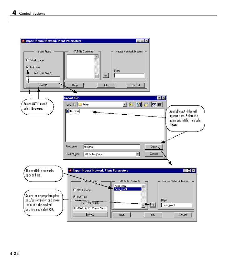
4 Control Systems
4-34
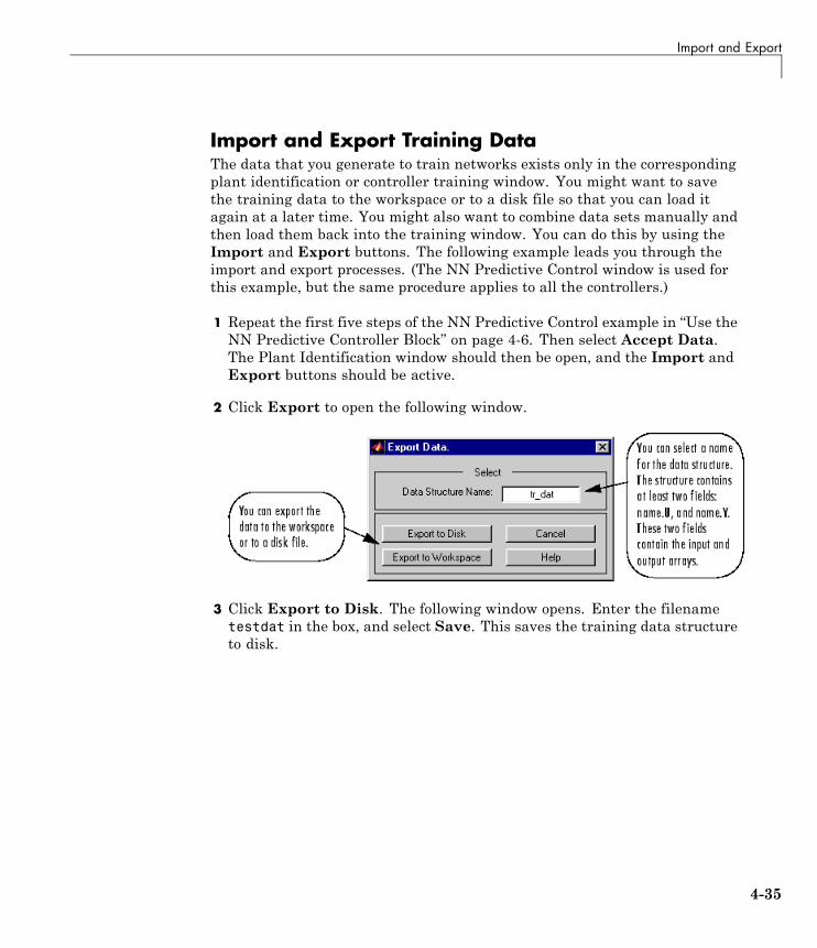
Import and Export
Import and Export Training DataThe data that you generate to train networks exists only in the correspondingplant identification or controller training window. You might want to savethe training data to the workspace or to a disk file so that you can load itagain at a later time. You might also want to combine data sets manually andthen load them back into the training window. You can do this by using theImport and Export buttons. The following example leads you through theimport and export processes. (The NN Predictive Control window is used forthis example, but the same procedure applies to all the controllers.)
1 Repeat the first five steps of the NN Predictive Control example in “Use theNN Predictive Controller Block” on page 4-6. Then select Accept Data.The Plant Identification window should then be open, and the Import andExport buttons should be active.
2 Click Export to open the following window.
3 Click Export to Disk. The following window opens. Enter the filenametestdat in the box, and select Save. This saves the training data structureto disk.
4-35
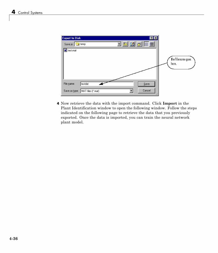
4 Control Systems
4 Now retrieve the data with the import command. Click Import in thePlant Identification window to open the following window. Follow the stepsindicated on the following page to retrieve the data that you previouslyexported. Once the data is imported, you can train the neural networkplant model.
4-36
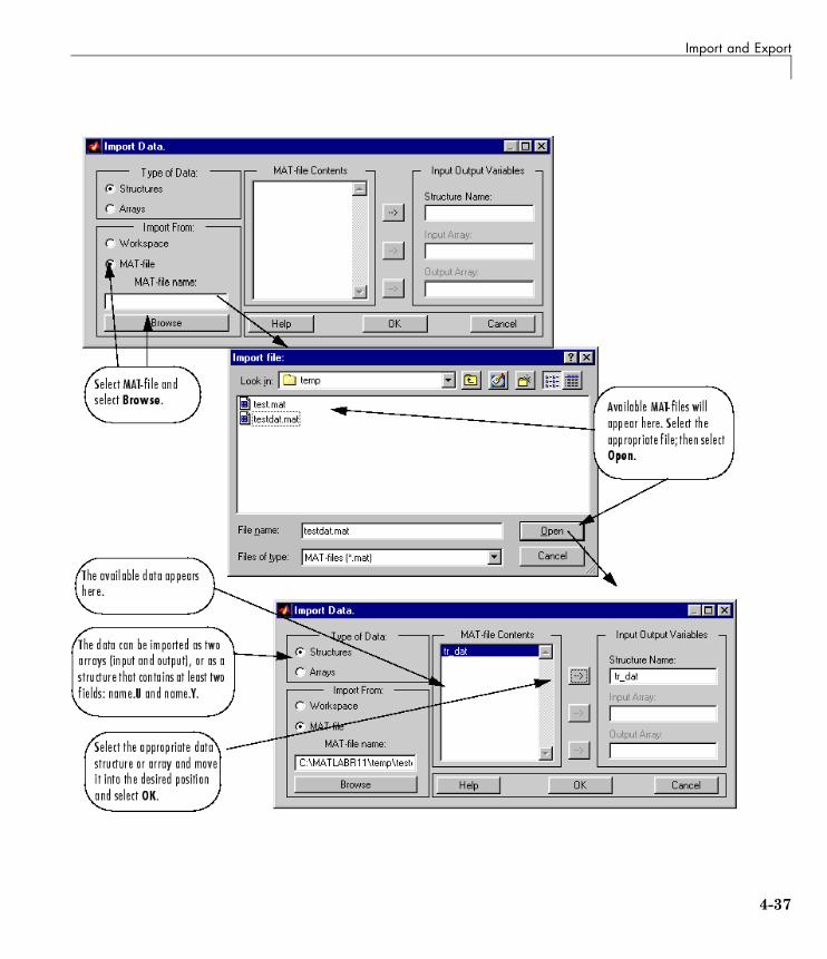
Import and Export
4-37

4 Control Systems
4-38

5
Radial Basis Networks
• “Introduction” on page 5-2
• “Radial Basis Functions” on page 5-3
• “Probabilistic Neural Networks” on page 5-10
• “Generalized Regression Networks” on page 5-13
5 Radial Basis Networks
IntroductionRadial basis networks can require more neurons than standard feedforwardbackpropagation networks, but often they can be designed in a fraction of thetime it takes to train standard feedforward networks. They work best whenmany training vectors are available.
You might want to consult the following paper on this subject: Chen,S., C.F.N. Cowan, and P.M. Grant, “Orthogonal Least Squares LearningAlgorithm for Radial Basis Function Networks,” IEEE Transactions onNeural Networks, Vol. 2, No. 2, March 1991, pp. 302–309.
This chapter discusses two variants of radial basis networks, generalizedregression networks (GRNN) and probabilistic neural networks (PNN). Youcan read about them in P.D. Wasserman, Advanced Methods in NeuralComputing, New York: Van Nostrand Reinhold, 1993, on pp. 155–61 andpp. 35–55, respectively.
Important Radial Basis FunctionsRadial basis networks can be designed with either newrbe or newrb. GRNNsand PNNs can be designed with newgrnn and newpnn, respectively.
5-2
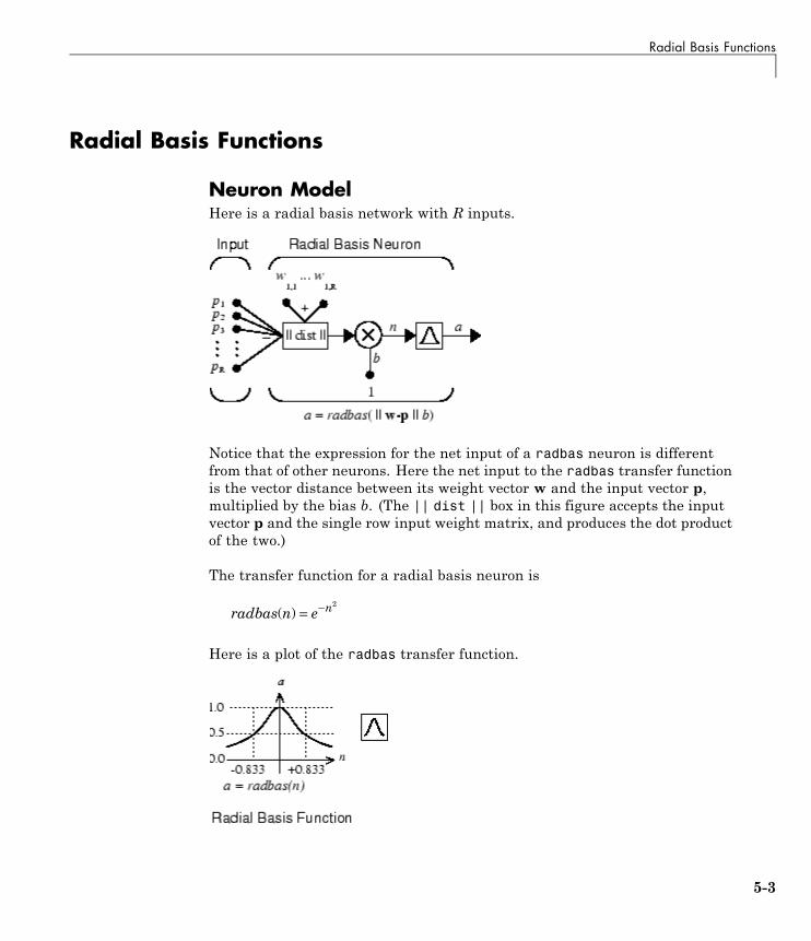
Radial Basis Functions
Radial Basis Functions
Neuron ModelHere is a radial basis network with R inputs.
Notice that the expression for the net input of a radbas neuron is differentfrom that of other neurons. Here the net input to the radbas transfer functionis the vector distance between its weight vector w and the input vector p,multiplied by the bias b. (The || dist || box in this figure accepts the inputvector p and the single row input weight matrix, and produces the dot productof the two.)
The transfer function for a radial basis neuron is
radbas n e n( ) = − 2
Here is a plot of the radbas transfer function.
5-3
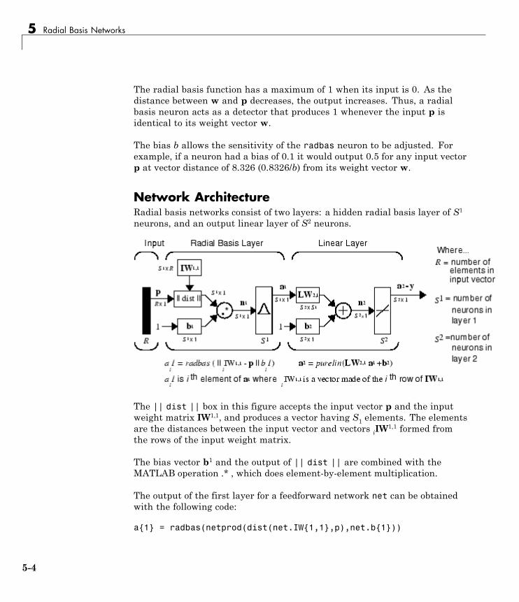
5 Radial Basis Networks
The radial basis function has a maximum of 1 when its input is 0. As thedistance between w and p decreases, the output increases. Thus, a radialbasis neuron acts as a detector that produces 1 whenever the input p isidentical to its weight vector w.
The bias b allows the sensitivity of the radbas neuron to be adjusted. Forexample, if a neuron had a bias of 0.1 it would output 0.5 for any input vectorp at vector distance of 8.326 (0.8326/b) from its weight vector w.
Network ArchitectureRadial basis networks consist of two layers: a hidden radial basis layer of S1
neurons, and an output linear layer of S2 neurons.
The || dist || box in this figure accepts the input vector p and the inputweight matrix IW1,1, and produces a vector having S1 elements. The elementsare the distances between the input vector and vectors iIW
1,1 formed fromthe rows of the input weight matrix.
The bias vector b1 and the output of || dist || are combined with theMATLAB operation .* , which does element-by-element multiplication.
The output of the first layer for a feedforward network net can be obtainedwith the following code:
a{1} = radbas(netprod(dist(net.IW{1,1},p),net.b{1}))
5-4

Radial Basis Functions
Fortunately, you won’t have to write such lines of code. All the details ofdesigning this network are built into design functions newrbe and newrb, andyou can obtain their outputs with sim.
You can understand how this network behaves by following an input vector pthrough the network to the output a2. If you present an input vector to such anetwork, each neuron in the radial basis layer will output a value according tohow close the input vector is to each neuron’s weight vector.
Thus, radial basis neurons with weight vectors quite different from the inputvector p have outputs near zero. These small outputs have only a negligibleeffect on the linear output neurons.
In contrast, a radial basis neuron with a weight vector close to the input vectorp produces a value near 1. If a neuron has an output of 1, its output weightsin the second layer pass their values to the linear neurons in the second layer.
In fact, if only one radial basis neuron had an output of 1, and all others hadoutputs of 0s (or very close to 0), the output of the linear layer would be theactive neuron’s output weights. This would, however, be an extreme case.Typically several neurons are always firing, to varying degrees.
Now look in detail at how the first layer operates. Each neuron’s weightedinput is the distance between the input vector and its weight vector, calculatedwith dist. Each neuron’s net input is the element-by-element product of itsweighted input with its bias, calculated with netprod. Each neuron’s outputis its net input passed through radbas. If a neuron’s weight vector is equal tothe input vector (transposed), its weighted input is 0, its net input is 0, andits output is 1. If a neuron’s weight vector is a distance of spread from theinput vector, its weighted input is spread, its net input is sqrt(−log(.5)) (or0.8326), therefore its output is 0.5.
Exact Design (newrbe)You can design radial basis networks with the function newrbe. This functioncan produce a network with zero error on training vectors. It is called inthe following way:
net = newrbe(P,T,SPREAD)
5-5
5 Radial Basis Networks
The function newrbe takes matrices of input vectors P and target vectorsT, and a spread constant SPREAD for the radial basis layer, and returns anetwork with weights and biases such that the outputs are exactly T whenthe inputs are P.
This function newrbe creates as many radbas neurons as there are inputvectors in P, and sets the first-layer weights to P'. Thus, there is a layer ofradbas neurons in which each neuron acts as a detector for a different inputvector. If there are Q input vectors, then there will be Q neurons.
Each bias in the first layer is set to 0.8326/SPREAD. This gives radial basisfunctions that cross 0.5 at weighted inputs of +/− SPREAD. This determinesthe width of an area in the input space to which each neuron responds. IfSPREAD is 4, then each radbas neuron will respond with 0.5 or more to anyinput vectors within a vector distance of 4 from their weight vector. SPREADshould be large enough that neurons respond strongly to overlapping regionsof the input space.
The second-layer weights IW 2,1 (or in code, IW{2,1}) and biases b2 (or in code,b{2}) are found by simulating the first-layer outputs a1 (A{1}), and thensolving the following linear expression:
[W{2,1} b{2}] * [A{1}; ones(1,Q)] = T
You know the inputs to the second layer (A{1}) and the target (T), and thelayer is linear. You can use the following code to calculate the weights andbiases of the second layer to minimize the sum-squared error.
Wb = T/[A{1}; ones(1,Q)]
Here Wb contains both weights and biases, with the biases in the last column.The sum-squared error is always 0, as explained below.
There is a problem with C constraints (input/target pairs) and each neuronhas C +1 variables (the C weights from the C radbas neurons, and a bias). Alinear problem with C constraints and more than C variables has an infinitenumber of zero error solutions.
5-6
Radial Basis Functions
Thus, newrbe creates a network with zero error on training vectors. The onlycondition required is to make sure that SPREAD is large enough that the activeinput regions of the radbas neurons overlap enough so that several radbasneurons always have fairly large outputs at any given moment. This makesthe network function smoother and results in better generalization for newinput vectors occurring between input vectors used in the design. (However,SPREAD should not be so large that each neuron is effectively responding inthe same large area of the input space.)
The drawback to newrbe is that it produces a network with as many hiddenneurons as there are input vectors. For this reason, newrbe does not returnan acceptable solution when many input vectors are needed to properly definea network, as is typically the case.
More Efficient Design (newrb)The function newrb iteratively creates a radial basis network one neuron ata time. Neurons are added to the network until the sum-squared error fallsbeneath an error goal or a maximum number of neurons has been reached.The call for this function is
net = newrb(P,T,GOAL,SPREAD)
The function newrb takes matrices of input and target vectors P and T, anddesign parameters GOAL and SPREAD, and returns the desired network.
The design method of newrb is similar to that of newrbe. The difference isthat newrb creates neurons one at a time. At each iteration the input vectorthat results in lowering the network error the most is used to create a radbasneuron. The error of the new network is checked, and if low enough newrbis finished. Otherwise the next neuron is added. This procedure is repeateduntil the error goal is met or the maximum number of neurons is reached.
As with newrbe, it is important that the spread parameter be large enoughthat the radbas neurons respond to overlapping regions of the input space,but not so large that all the neurons respond in essentially the same manner.
Why not always use a radial basis network instead of a standard feedforwardnetwork? Radial basis networks, even when designed efficiently with newrbe,
5-7
5 Radial Basis Networks
tend to have many times more neurons than a comparable feedforwardnetwork with tansig or logsig neurons in the hidden layer.
This is because sigmoid neurons can have outputs over a large region of theinput space, while radbas neurons only respond to relatively small regionsof the input space. The result is that the larger the input space (in terms ofnumber of inputs, and the ranges those inputs vary over) the more radbasneurons required.
On the other hand, designing a radial basis network often takes much lesstime than training a sigmoid/linear network, and can sometimes result infewer neurons’ being used, as can be seen in the next example.
ExamplesThe example demorb1 shows how a radial basis network is used to fit afunction. Here the problem is solved with only five neurons.
Examples demorb3 and demorb4 examine how the spread constant affects thedesign process for radial basis networks.
In demorb3, a radial basis network is designed to solve the same problem asin demorb1. However, this time the spread constant used is 0.01. Thus, eachradial basis neuron returns 0.5 or lower for any input vector with a distanceof 0.01 or more from its weight vector.
Because the training inputs occur at intervals of 0.1, no two radial basisneurons have a strong output for any given input.
demorb3 showed that having too small a spread constant can result in asolution that does not generalize from the input/target vectors used in thedesign. Example demorb4 shows the opposite problem. If the spread constantis large enough, the radial basis neurons will output large values (near 1.0)for all the inputs used to design the network.
If all the radial basis neurons always output 1, any information presented tothe network becomes lost. No matter what the input, the second layer outputs1’s. The function newrb will attempt to find a network, but cannot because ofnumerical problems that arise in this situation.
5-8

Radial Basis Functions
The moral of the story is, choose a spread constant larger than the distancebetween adjacent input vectors, so as to get good generalization, but smallerthan the distance across the whole input space.
For this problem that would mean picking a spread constant greater than0.1, the interval between inputs, and less than 2, the distance between theleftmost and rightmost inputs.
5-9
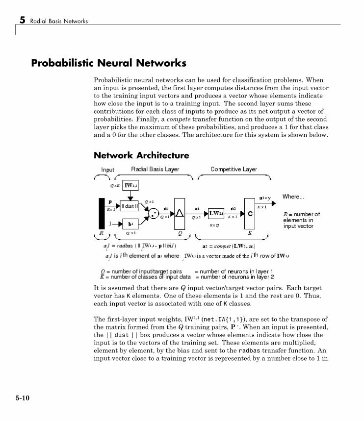
5 Radial Basis Networks
Probabilistic Neural NetworksProbabilistic neural networks can be used for classification problems. Whenan input is presented, the first layer computes distances from the input vectorto the training input vectors and produces a vector whose elements indicatehow close the input is to a training input. The second layer sums thesecontributions for each class of inputs to produce as its net output a vector ofprobabilities. Finally, a compete transfer function on the output of the secondlayer picks the maximum of these probabilities, and produces a 1 for that classand a 0 for the other classes. The architecture for this system is shown below.
Network Architecture
It is assumed that there are Q input vector/target vector pairs. Each targetvector has K elements. One of these elements is 1 and the rest are 0. Thus,each input vector is associated with one of K classes.
The first-layer input weights, IW1,1 (net.IW{1,1}), are set to the transpose ofthe matrix formed from the Q training pairs, P'. When an input is presented,the || dist || box produces a vector whose elements indicate how close theinput is to the vectors of the training set. These elements are multiplied,element by element, by the bias and sent to the radbas transfer function. Aninput vector close to a training vector is represented by a number close to 1 in
5-10
Probabilistic Neural Networks
the output vector a1. If an input is close to several training vectors of a singleclass, it is represented by several elements of a1 that are close to 1.
The second-layer weights, LW1,2 (net.LW{2,1}), are set to the matrix T oftarget vectors. Each vector has a 1 only in the row associated with thatparticular class of input, and 0s elsewhere. (Use function ind2vec to createthe proper vectors.) The multiplication Ta1 sums the elements of a1 dueto each of the K input classes. Finally, the second-layer transfer function,compet, produces a 1 corresponding to the largest element of n2, and 0selsewhere. Thus, the network classifies the input vector into a specific K classbecause that class has the maximum probability of being correct.
Design (newpnn)You can use the function newpnn to create a PNN. For instance, suppose thatseven input vectors and their corresponding targets are
P = [0 0;1 1;0 3;1 4;3 1;4 1;4 3]'
which yields
P =0 1 0 1 3 4 40 1 3 4 1 1 3
Tc = [1 1 2 2 3 3 3]
which yields
Tc =1 1 2 2 3 3 3
You need a target matrix with 1s in the right places. You can get it with thefunction ind2vec. It gives a matrix with 0s except at the correct spots. Soexecute
T = ind2vec(Tc)
which gives
T =(1,1) 1
5-11
5 Radial Basis Networks
(1,2) 1(2,3) 1(2,4) 1(3,5) 1(3,6) 1(3,7) 1
Now you can create a network and simulate it, using the input P to make surethat it does produce the correct classifications. Use the function vec2ind toconvert the output Y into a row Yc to make the classifications clear.
net = newpnn(P,T);Y = sim(net,P);Yc = vec2ind(Y)
This produces
Yc =1 1 2 2 3 3 3
You might try classifying vectors other than those that were used to designthe network. Try to classify the vectors shown below in P2.
P2 = [1 4;0 1;5 2]'P2 =
1 0 54 1 2
Can you guess how these vectors will be classified? If you run the simulationand plot the vectors as before, you get
Yc =2 1 3
These results look good, for these test vectors were quite close to membersof classes 2, 1, and 3, respectively. The network has managed to generalizeits operation to properly classify vectors other than those used to design thenetwork.
You might want to try demopnn1. It shows how to design a PNN, and how thenetwork can successfully classify a vector not used in the design.
5-12
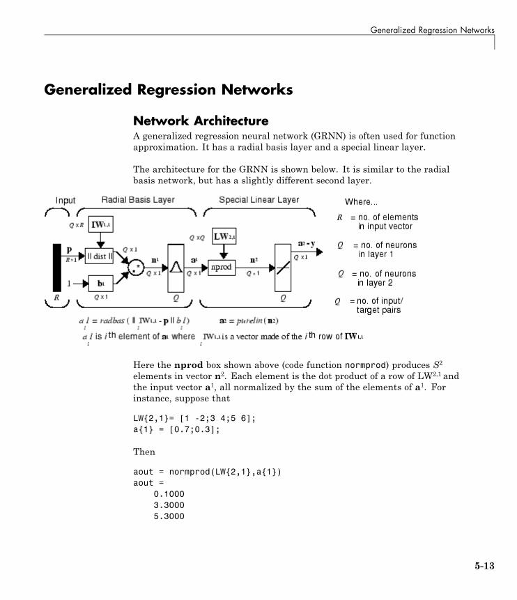
Generalized Regression Networks
Generalized Regression Networks
Network ArchitectureA generalized regression neural network (GRNN) is often used for functionapproximation. It has a radial basis layer and a special linear layer.
The architecture for the GRNN is shown below. It is similar to the radialbasis network, but has a slightly different second layer.
Here the nprod box shown above (code function normprod) produces S2
elements in vector n2. Each element is the dot product of a row of LW2,1 andthe input vector a1, all normalized by the sum of the elements of a1. Forinstance, suppose that
LW{2,1}= [1 -2;3 4;5 6];a{1} = [0.7;0.3];
Then
aout = normprod(LW{2,1},a{1})aout =
0.10003.30005.3000
5-13
5 Radial Basis Networks
The first layer is just like that for newrbe networks. It has as many neuronsas there are input/ target vectors in P. Specifically, the first-layer weightsare set to P'. The bias b1 is set to a column vector of 0.8326/SPREAD. Theuser chooses SPREAD, the distance an input vector must be from a neuron’sweight vector to be 0.5.
Again, the first layer operates just like the newrbe radial basis layer describedpreviously. Each neuron’s weighted input is the distance between the inputvector and its weight vector, calculated with dist. Each neuron’s net inputis the product of its weighted input with its bias, calculated with netprod.Each neuron’s output is its net input passed through radbas. If a neuron’sweight vector is equal to the input vector (transposed), its weighted input willbe 0, its net input will be 0, and its output will be 1. If a neuron’s weightvector is a distance of spread from the input vector, its weighted input willbe spread, and its net input will be sqrt(−log(.5)) (or 0.8326). Therefore itsoutput will be 0.5.
The second layer also has as many neurons as input/target vectors, but hereLW{2,1} is set to T.
Suppose you have an input vector p close to pi, one of the input vectors amongthe input vector/target pairs used in designing layer 1 weights. This input pproduces a layer 1 ai output close to 1. This leads to a layer 2 output close toti, one of the targets used to form layer 2 weights.
A larger spread leads to a large area around the input vector where layer 1neurons will respond with significant outputs. Therefore if spread is smallthe radial basis function is very steep, so that the neuron with the weightvector closest to the input will have a much larger output than other neurons.The network tends to respond with the target vector associated with thenearest design input vector.
As spread becomes larger the radial basis function’s slope becomes smootherand several neurons can respond to an input vector. The network then actsas if it is taking a weighted average between target vectors whose designinput vectors are closest to the new input vector. As spread becomes largermore and more neurons contribute to the average, with the result that thenetwork function becomes smoother.
5-14
Generalized Regression Networks
Design (newgrnn)You can use the function newgrnn to create a GRNN. For instance, supposethat three input and three target vectors are defined as
P = [4 5 6];T = [1.5 3.6 6.7];
You can now obtain a GRNN with
net = newgrnn(P,T);
and simulate it with
P = 4.5;v = sim(net,P);
You might want to try demogrn1. It shows how to approximate a functionwith a GRNN.
Function Description
compet Competitive transfer function.
dist Euclidean distance weight function.
dotprod Dot product weight function.
ind2vec Convert indices to vectors.
negdist Negative Euclidean distance weight function.
netprod Product net input function.
newgrnn Design a generalized regression neural network.
newpnn Design a probabilistic neural network.
newrb Design a radial basis network.
newrbe Design an exact radial basis network.
normprod Normalized dot product weight function.
radbas Radial basis transfer function.
vec2ind Convert vectors to indices.
5-15

5 Radial Basis Networks
5-16

6
Self-Organizing andLearning VectorQuantization Nets
• “Introduction” on page 6-2
• “Competitive Learning” on page 6-3
• “Self-Organizing Feature Maps” on page 6-10
• “Learning Vector Quantization Networks” on page 6-37
6 Self-Organizing and Learning Vector Quantization Nets
IntroductionSelf-organizing in networks is one of the most fascinating topics in the neuralnetwork field. Such networks can learn to detect regularities and correlationsin their input and adapt their future responses to that input accordingly.The neurons of competitive networks learn to recognize groups of similarinput vectors. Self-organizing maps learn to recognize groups of similar inputvectors in such a way that neurons physically near each other in the neuronlayer respond to similar input vectors. Self-organizing maps do not havetarget vectors, since their purpose is to divide the input vectors into clustersof similar vectors. There is no desired output for these types of networks.
Learning vector quantization (LVQ) is a method for training competitivelayers in a supervised manner (with target outputs). A competitive layerautomatically learns to classify input vectors. However, the classes thatthe competitive layer finds are dependent only on the distance betweeninput vectors. If two input vectors are very similar, the competitive layerprobably will put them in the same class. There is no mechanism in a strictlycompetitive layer design to say whether or not any two input vectors are inthe same class or different classes.
LVQ networks, on the other hand, learn to classify input vectors into targetclasses chosen by the user.
You might consult the following reference: Kohonen, T., Self-Organizationand Associative Memory, 2nd Edition, Berlin: Springer-Verlag, 1987.
Important Self-Organizing and LVQ FunctionsYou can create competitive layers and self-organizing maps with competlayerand selforgmap, respectively.
You can create an LVQ network with the function newlvq.
6-2
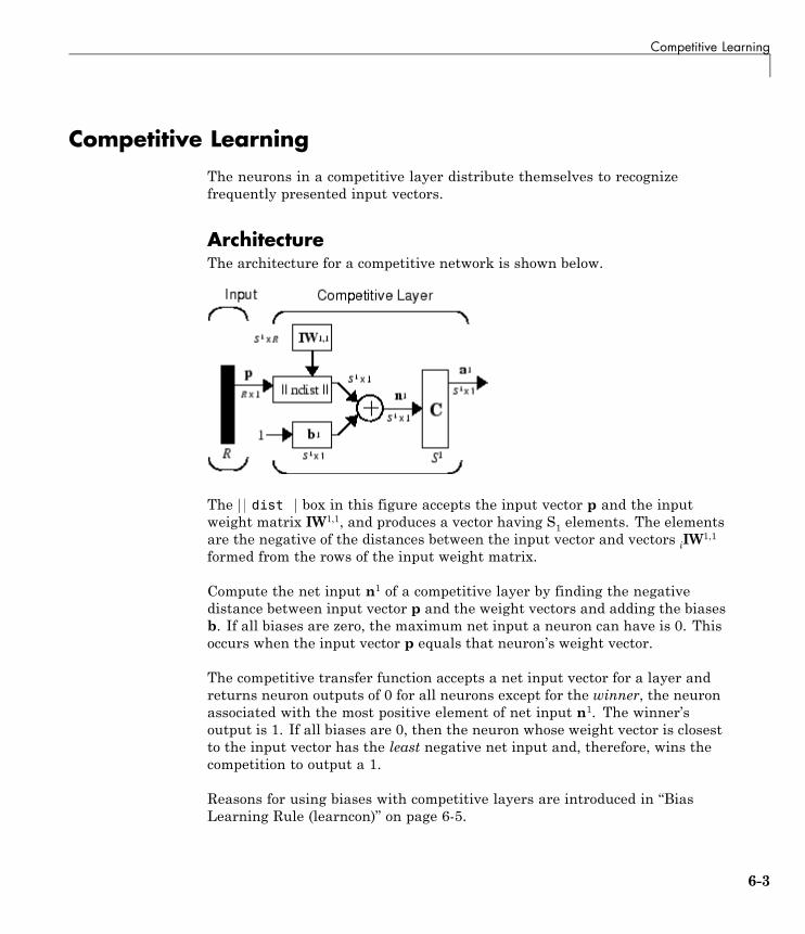
Competitive Learning
Competitive LearningThe neurons in a competitive layer distribute themselves to recognizefrequently presented input vectors.
ArchitectureThe architecture for a competitive network is shown below.
The dist box in this figure accepts the input vector p and the inputweight matrix IW1,1, and produces a vector having S1 elements. The elementsare the negative of the distances between the input vector and vectors iIW
1,1
formed from the rows of the input weight matrix.
Compute the net input n1 of a competitive layer by finding the negativedistance between input vector p and the weight vectors and adding the biasesb. If all biases are zero, the maximum net input a neuron can have is 0. Thisoccurs when the input vector p equals that neuron’s weight vector.
The competitive transfer function accepts a net input vector for a layer andreturns neuron outputs of 0 for all neurons except for the winner, the neuronassociated with the most positive element of net input n1. The winner’soutput is 1. If all biases are 0, then the neuron whose weight vector is closestto the input vector has the least negative net input and, therefore, wins thecompetition to output a 1.
Reasons for using biases with competitive layers are introduced in “BiasLearning Rule (learncon)” on page 6-5.
6-3
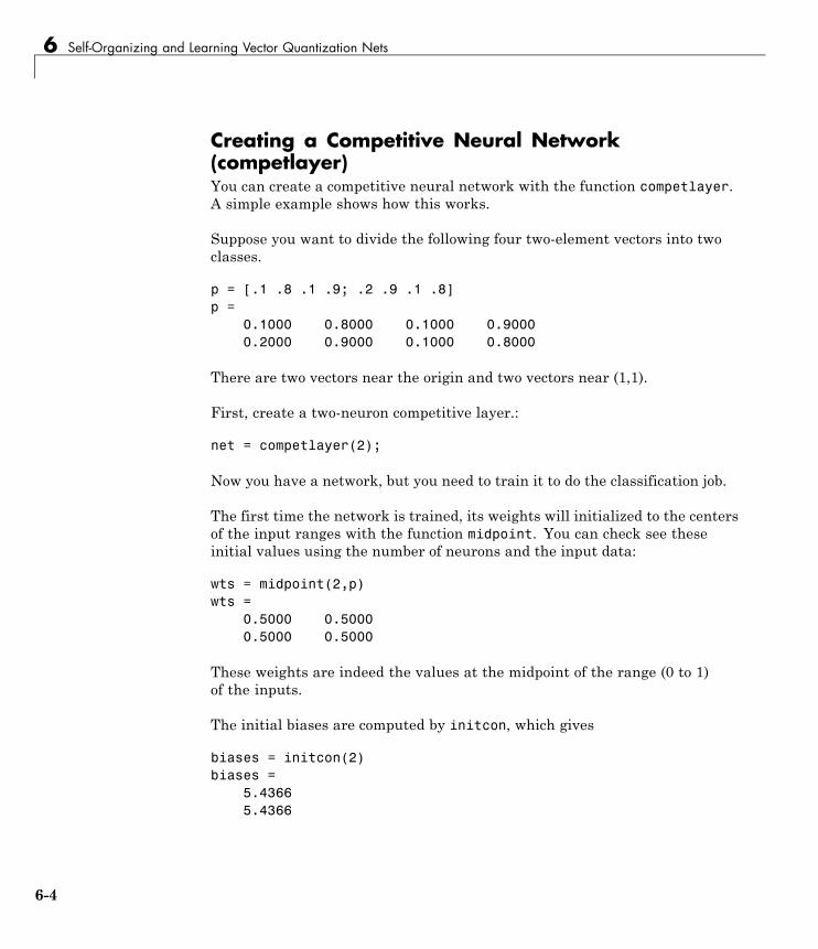
6 Self-Organizing and Learning Vector Quantization Nets
Creating a Competitive Neural Network(competlayer)You can create a competitive neural network with the function competlayer.A simple example shows how this works.
Suppose you want to divide the following four two-element vectors into twoclasses.
p = [.1 .8 .1 .9; .2 .9 .1 .8]p =
0.1000 0.8000 0.1000 0.90000.2000 0.9000 0.1000 0.8000
There are two vectors near the origin and two vectors near (1,1).
First, create a two-neuron competitive layer.:
net = competlayer(2);
Now you have a network, but you need to train it to do the classification job.
The first time the network is trained, its weights will initialized to the centersof the input ranges with the function midpoint. You can check see theseinitial values using the number of neurons and the input data:
wts = midpoint(2,p)wts =
0.5000 0.50000.5000 0.5000
These weights are indeed the values at the midpoint of the range (0 to 1)of the inputs.
The initial biases are computed by initcon, which gives
biases = initcon(2)biases =
5.43665.4366
6-4
Competitive Learning
Recall that each neuron competes to respond to an input vector p. If the biasesare all 0, the neuron whose weight vector is closest to p gets the highest netinput and, therefore, wins the competition, and outputs 1. All other neuronsoutput 0. You want to adjust the winning neuron so as to move it closer to theinput. A learning rule to do this is discussed in the next section.
Kohonen Learning Rule (learnk)The weights of the winning neuron (a row of the input weight matrix) areadjusted with the Kohonen learning rule. Supposing that the ith neuronwins, the elements of the ith row of the input weight matrix are adjustedas shown below.
i i iq q q qIW IW p IW1 1 1 1 1 11 1, , ,( ) ( ) ( ( ) ( ))= − + − −
The Kohonen rule allows the weights of a neuron to learn an input vector, andbecause of this it is useful in recognition applications.
Thus, the neuron whose weight vector was closest to the input vector isupdated to be even closer. The result is that the winning neuron is morelikely to win the competition the next time a similar vector is presented, andless likely to win when a very different input vector is presented. As moreand more inputs are presented, each neuron in the layer closest to a groupof input vectors soon adjusts its weight vector toward those input vectors.Eventually, if there are enough neurons, every cluster of similar input vectorswill have a neuron that outputs 1 when a vector in the cluster is presented,while outputting a 0 at all other times. Thus, the competitive network learnsto categorize the input vectors it sees.
The function learnk is used to perform the Kohonen learning rule in thistoolbox.
Bias Learning Rule (learncon)One of the limitations of competitive networks is that some neurons mightnot always be allocated. In other words, some neuron weight vectors mightstart out far from any input vectors and never win the competition, no matterhow long the training is continued. The result is that their weights do not get
6-5
6 Self-Organizing and Learning Vector Quantization Nets
to learn and they never win. These unfortunate neurons, referred to as deadneurons, never perform a useful function.
To stop this, use biases to give neurons that only win the competition rarely(if ever) an advantage over neurons that win often. A positive bias, added tothe negative distance, makes a distant neuron more likely to win.
To do this job a running average of neuron outputs is kept. It is equivalent tothe percentages of times each output is 1. This average is used to update thebiases with the learning function learncon so that the biases of frequentlyactive neurons become smaller, and biases of infrequently active neuronsbecome larger.
As the biases of infrequently active neurons increase, the input space towhich those neurons respond increases. As that input space increases, theinfrequently active neuron responds and moves toward more input vectors.Eventually, the neuron responds to the same number of vectors as otherneurons.
This has two good effects. First, if a neuron never wins a competition becauseits weights are far from any of the input vectors, its bias eventually becomeslarge enough so that it can win. When this happens, it moves toward somegroup of input vectors. Once the neuron’s weights have moved into a group ofinput vectors and the neuron is winning consistently, its bias will decrease to0. Thus, the problem of dead neurons is resolved.
The second advantage of biases is that they force each neuron to classifyroughly the same percentage of input vectors. Thus, if a region of the inputspace is associated with a larger number of input vectors than another region,the more densely filled region will attract more neurons and be classified intosmaller subsections.
The learning rates for learncon are typically set an order of magnitude ormore smaller than for learnk to make sure that the running average isaccurate.
TrainingNow train the network for 500 epochs. You can use either train or adapt.
6-6
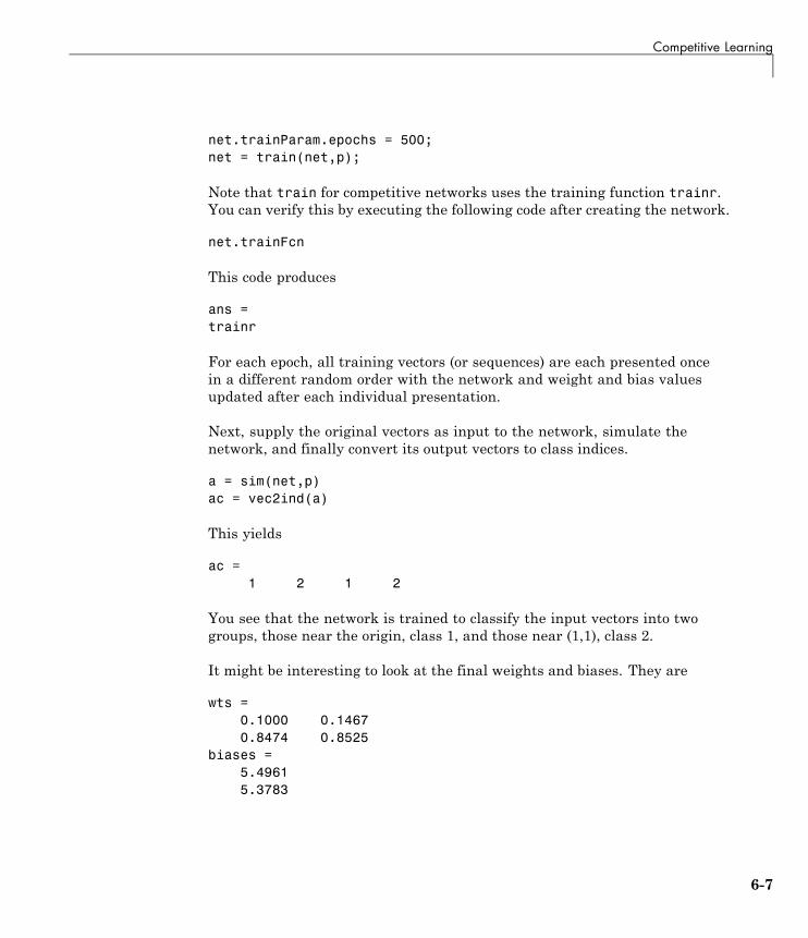
Competitive Learning
net.trainParam.epochs = 500;net = train(net,p);
Note that train for competitive networks uses the training function trainr.You can verify this by executing the following code after creating the network.
net.trainFcn
This code produces
ans =trainr
For each epoch, all training vectors (or sequences) are each presented oncein a different random order with the network and weight and bias valuesupdated after each individual presentation.
Next, supply the original vectors as input to the network, simulate thenetwork, and finally convert its output vectors to class indices.
a = sim(net,p)ac = vec2ind(a)
This yields
ac =1 2 1 2
You see that the network is trained to classify the input vectors into twogroups, those near the origin, class 1, and those near (1,1), class 2.
It might be interesting to look at the final weights and biases. They are
wts =0.1000 0.14670.8474 0.8525
biases =5.49615.3783
6-7
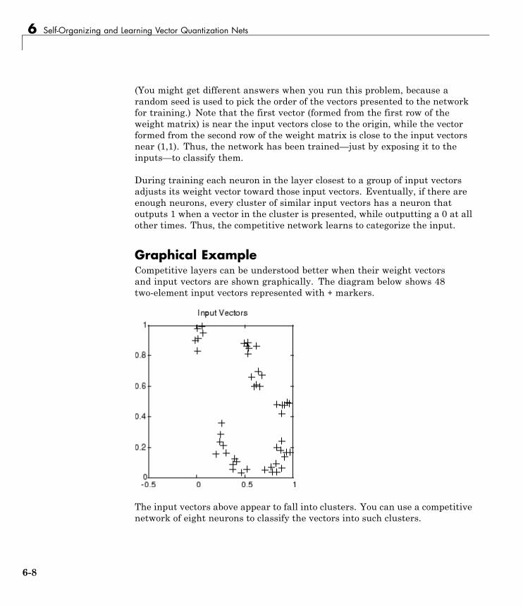
6 Self-Organizing and Learning Vector Quantization Nets
(You might get different answers when you run this problem, because arandom seed is used to pick the order of the vectors presented to the networkfor training.) Note that the first vector (formed from the first row of theweight matrix) is near the input vectors close to the origin, while the vectorformed from the second row of the weight matrix is close to the input vectorsnear (1,1). Thus, the network has been trained—just by exposing it to theinputs—to classify them.
During training each neuron in the layer closest to a group of input vectorsadjusts its weight vector toward those input vectors. Eventually, if there areenough neurons, every cluster of similar input vectors has a neuron thatoutputs 1 when a vector in the cluster is presented, while outputting a 0 at allother times. Thus, the competitive network learns to categorize the input.
Graphical ExampleCompetitive layers can be understood better when their weight vectorsand input vectors are shown graphically. The diagram below shows 48two-element input vectors represented with + markers.
The input vectors above appear to fall into clusters. You can use a competitivenetwork of eight neurons to classify the vectors into such clusters.
6-8

Competitive Learning
Try democ1 to see a dynamic example of competitive learning.
6-9
6 Self-Organizing and Learning Vector Quantization Nets
Self-Organizing Feature MapsSelf-organizing feature maps (SOFM) learn to classify input vectors accordingto how they are grouped in the input space. They differ from competitivelayers in that neighboring neurons in the self-organizing map learn torecognize neighboring sections of the input space. Thus, self-organizing mapslearn both the distribution (as do competitive layers) and topology of the inputvectors they are trained on.
The neurons in the layer of an SOFM are arranged originally in physicalpositions according to a topology function. The function gridtop, hextop, orrandtop can arrange the neurons in a grid, hexagonal, or random topology.Distances between neurons are calculated from their positions with a distancefunction. There are four distance functions, dist, boxdist, linkdist, andmandist. Link distance is the most common. These topology and distancefunctions are described in “Topologies (gridtop, hextop, randtop)” on page 6-11and “Distance Functions (dist, linkdist, mandist, boxdist)” on page 6-15.
Here a self-organizing feature map network identifies a winning neuron i*using the same procedure as employed by a competitive layer. However,instead of updating only the winning neuron, all neurons within a certainneighborhood Ni* (d) of the winning neuron are updated, using the Kohonenrule. Specifically, all such neurons i Ni* (d) are adjusted as follows:
i i iq q q qw w p w( ) ( ) ( ( ) ( ))= − + − −1 1
or
i iq q qw w p( ) ( ) ( ) ( )= − − +1 1
Here the neighborhood Ni* (d) contains the indices for all of the neurons thatlie within a radius d of the winning neuron i*.
N d j d di ij( ) ,= ≤{ }
Thus, when a vector p is presented, the weights of the winning neuron andits close neighbors move toward p. Consequently, after many presentations,neighboring neurons have learned vectors similar to each other.
6-10
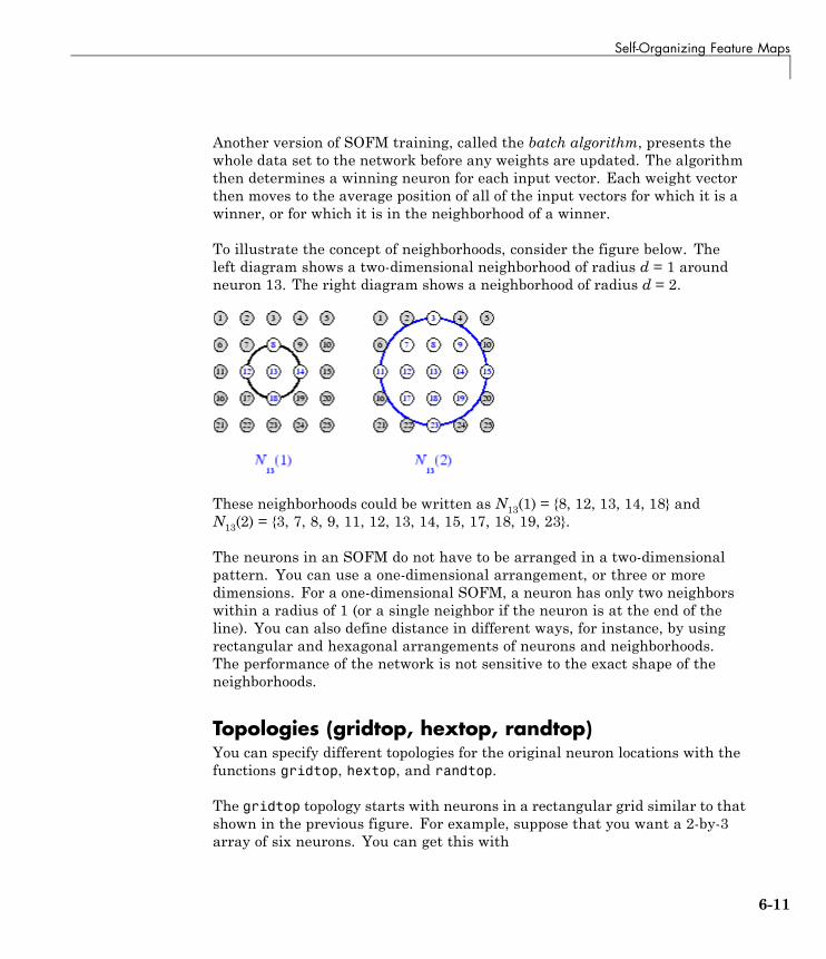
Self-Organizing Feature Maps
Another version of SOFM training, called the batch algorithm, presents thewhole data set to the network before any weights are updated. The algorithmthen determines a winning neuron for each input vector. Each weight vectorthen moves to the average position of all of the input vectors for which it is awinner, or for which it is in the neighborhood of a winner.
To illustrate the concept of neighborhoods, consider the figure below. Theleft diagram shows a two-dimensional neighborhood of radius d = 1 aroundneuron 13. The right diagram shows a neighborhood of radius d = 2.
These neighborhoods could be written as N13(1) = {8, 12, 13, 14, 18} andN13(2) = {3, 7, 8, 9, 11, 12, 13, 14, 15, 17, 18, 19, 23}.
The neurons in an SOFM do not have to be arranged in a two-dimensionalpattern. You can use a one-dimensional arrangement, or three or moredimensions. For a one-dimensional SOFM, a neuron has only two neighborswithin a radius of 1 (or a single neighbor if the neuron is at the end of theline). You can also define distance in different ways, for instance, by usingrectangular and hexagonal arrangements of neurons and neighborhoods.The performance of the network is not sensitive to the exact shape of theneighborhoods.
Topologies (gridtop, hextop, randtop)You can specify different topologies for the original neuron locations with thefunctions gridtop, hextop, and randtop.
The gridtop topology starts with neurons in a rectangular grid similar to thatshown in the previous figure. For example, suppose that you want a 2-by-3array of six neurons. You can get this with
6-11
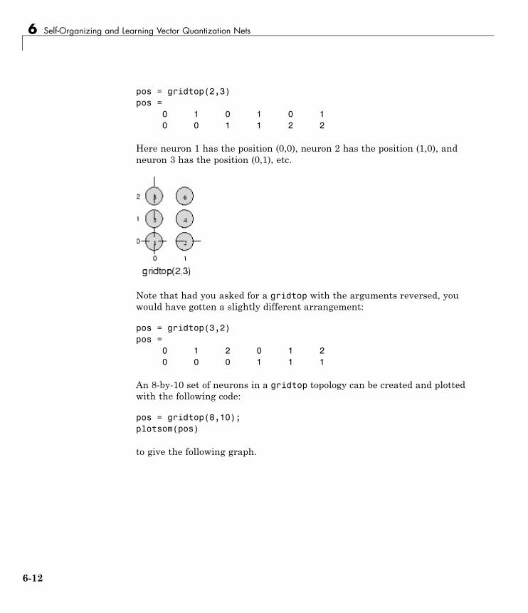
6 Self-Organizing and Learning Vector Quantization Nets
pos = gridtop(2,3)pos =
0 1 0 1 0 10 0 1 1 2 2
Here neuron 1 has the position (0,0), neuron 2 has the position (1,0), andneuron 3 has the position (0,1), etc.
Note that had you asked for a gridtop with the arguments reversed, youwould have gotten a slightly different arrangement:
pos = gridtop(3,2)pos =
0 1 2 0 1 20 0 0 1 1 1
An 8-by-10 set of neurons in a gridtop topology can be created and plottedwith the following code:
pos = gridtop(8,10);plotsom(pos)
to give the following graph.
6-12

Self-Organizing Feature Maps
As shown, the neurons in the gridtop topology do indeed lie on a grid.
The hextop function creates a similar set of neurons, but they are in ahexagonal pattern. A 2-by-3 pattern of hextop neurons is generated as follows:
pos = hextop(2,3)pos =
0 1.0000 0.5000 1.5000 0 1.00000 0 0.8660 0.8660 1.7321 1.7321
Note that hextop is the default pattern for SOM networks generated withselforgmap.
You can create and plot an 8-by-10 set of neurons in a hextop topology withthe following code:
6-13
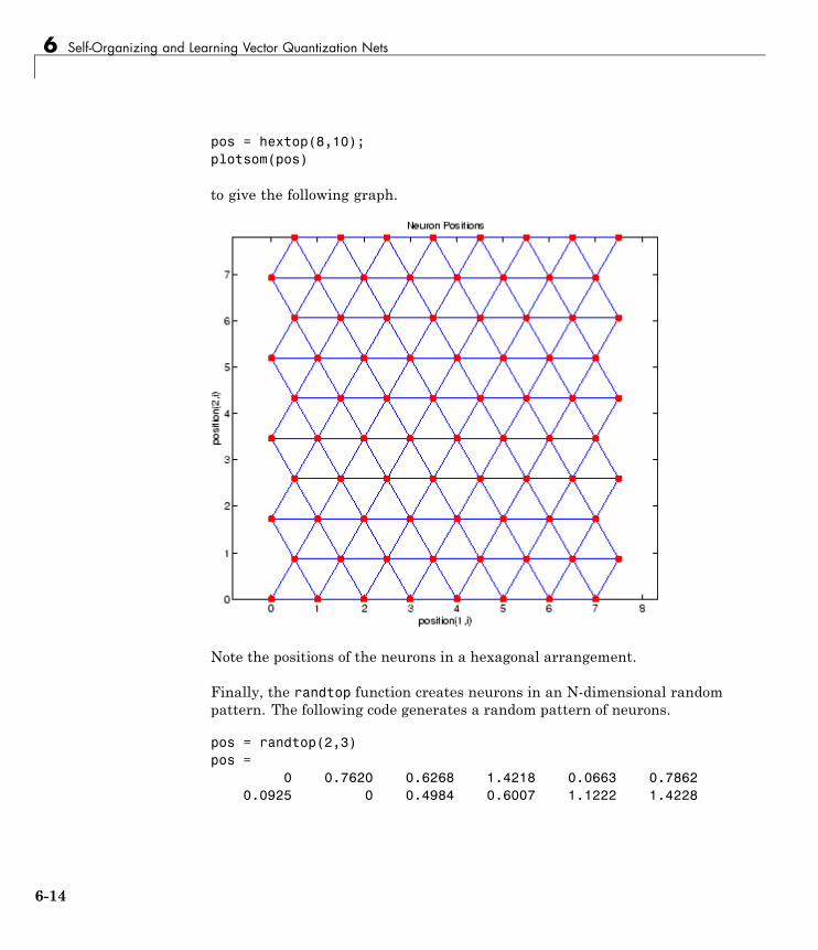
6 Self-Organizing and Learning Vector Quantization Nets
pos = hextop(8,10);plotsom(pos)
to give the following graph.
Note the positions of the neurons in a hexagonal arrangement.
Finally, the randtop function creates neurons in an N-dimensional randompattern. The following code generates a random pattern of neurons.
pos = randtop(2,3)pos =
0 0.7620 0.6268 1.4218 0.0663 0.78620.0925 0 0.4984 0.6007 1.1222 1.4228
6-14
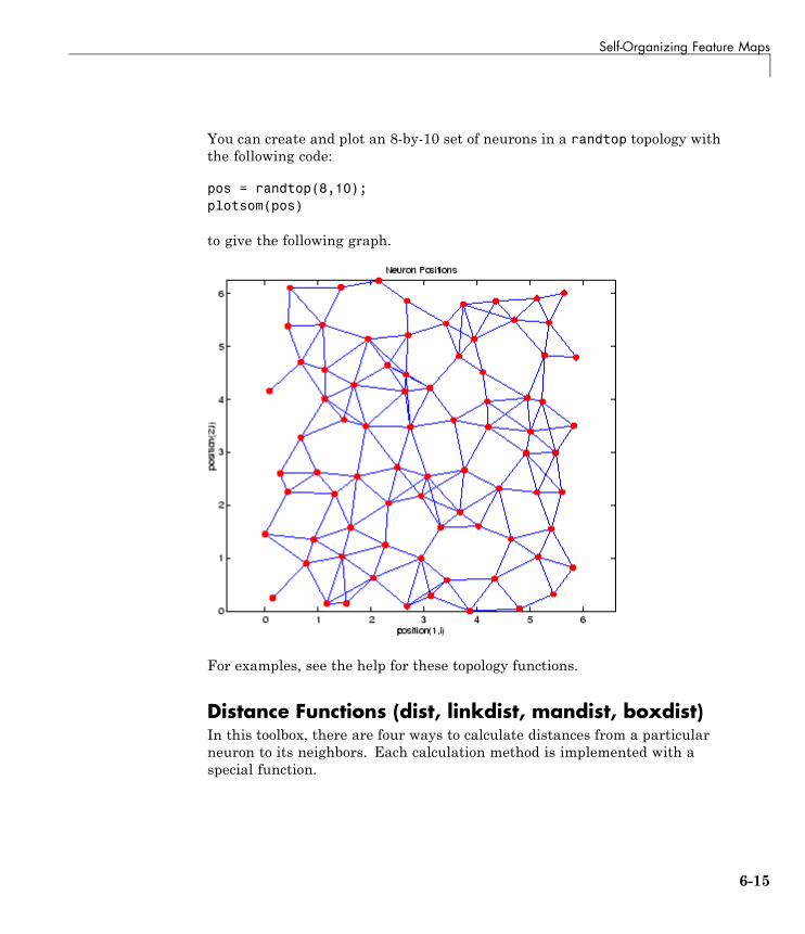
Self-Organizing Feature Maps
You can create and plot an 8-by-10 set of neurons in a randtop topology withthe following code:
pos = randtop(8,10);plotsom(pos)
to give the following graph.
For examples, see the help for these topology functions.
Distance Functions (dist, linkdist, mandist, boxdist)In this toolbox, there are four ways to calculate distances from a particularneuron to its neighbors. Each calculation method is implemented with aspecial function.
6-15
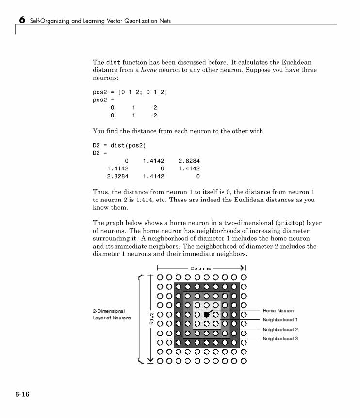
6 Self-Organizing and Learning Vector Quantization Nets
The dist function has been discussed before. It calculates the Euclideandistance from a home neuron to any other neuron. Suppose you have threeneurons:
pos2 = [0 1 2; 0 1 2]pos2 =
0 1 20 1 2
You find the distance from each neuron to the other with
D2 = dist(pos2)D2 =
0 1.4142 2.82841.4142 0 1.41422.8284 1.4142 0
Thus, the distance from neuron 1 to itself is 0, the distance from neuron 1to neuron 2 is 1.414, etc. These are indeed the Euclidean distances as youknow them.
The graph below shows a home neuron in a two-dimensional (gridtop) layerof neurons. The home neuron has neighborhoods of increasing diametersurrounding it. A neighborhood of diameter 1 includes the home neuronand its immediate neighbors. The neighborhood of diameter 2 includes thediameter 1 neurons and their immediate neighbors.
6-16
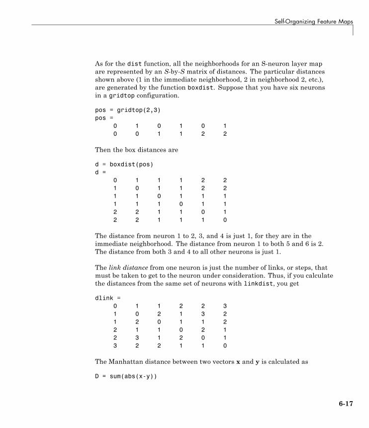
Self-Organizing Feature Maps
As for the dist function, all the neighborhoods for an S-neuron layer mapare represented by an S-by-S matrix of distances. The particular distancesshown above (1 in the immediate neighborhood, 2 in neighborhood 2, etc.),are generated by the function boxdist. Suppose that you have six neuronsin a gridtop configuration.
pos = gridtop(2,3)pos =
0 1 0 1 0 10 0 1 1 2 2
Then the box distances are
d = boxdist(pos)d =
0 1 1 1 2 21 0 1 1 2 21 1 0 1 1 11 1 1 0 1 12 2 1 1 0 12 2 1 1 1 0
The distance from neuron 1 to 2, 3, and 4 is just 1, for they are in theimmediate neighborhood. The distance from neuron 1 to both 5 and 6 is 2.The distance from both 3 and 4 to all other neurons is just 1.
The link distance from one neuron is just the number of links, or steps, thatmust be taken to get to the neuron under consideration. Thus, if you calculatethe distances from the same set of neurons with linkdist, you get
dlink =0 1 1 2 2 31 0 2 1 3 21 2 0 1 1 22 1 1 0 2 12 3 1 2 0 13 2 2 1 1 0
The Manhattan distance between two vectors x and y is calculated as
D = sum(abs(x-y))
6-17

6 Self-Organizing and Learning Vector Quantization Nets
Thus if you have
W1 = [1 2; 3 4; 5 6]W1 =
1 23 45 6
and
P1 = [1;1]P1 =
11
then you get for the distances
Z1 = mandist(W1,P1)Z1 =
159
The distances calculated with mandist do indeed follow the mathematicalexpression given above.
ArchitectureThe architecture for this SOFM is shown below.
6-18
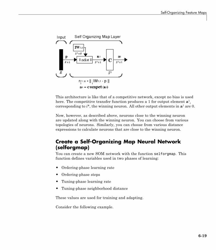
Self-Organizing Feature Maps
This architecture is like that of a competitive network, except no bias is usedhere. The competitive transfer function produces a 1 for output element a1icorresponding to i*, the winning neuron. All other output elements in a1 are 0.
Now, however, as described above, neurons close to the winning neuronare updated along with the winning neuron. You can choose from varioustopologies of neurons. Similarly, you can choose from various distanceexpressions to calculate neurons that are close to the winning neuron.
Create a Self-Organizing Map Neural Network(selforgmap)You can create a new SOM network with the function selforgmap. Thisfunction defines variables used in two phases of learning:
• Ordering-phase learning rate
• Ordering-phase steps
• Tuning-phase learning rate
• Tuning-phase neighborhood distance
These values are used for training and adapting.
Consider the following example.
6-19
6 Self-Organizing and Learning Vector Quantization Nets
Suppose that you want to create a network having input vectors with twoelements, and that you want to have six neurons in a hexagonal 2-by-3network. The code to obtain this network is
net = selforgmap([2,3]);
Suppose that the vectors to train on are
P = [.1 .3 1.2 1.1 1.8 1.7 .1 .3 1.2 1.1 1.8 1.7;...0.2 0.1 0.3 0.1 0.3 0.2 1.8 1.8 1.9 1.9 1.7 1.8]
You can configure the network to input the data and plot all of this with
net = configure(net,P);plotsompos(net,P);
to give
6-20
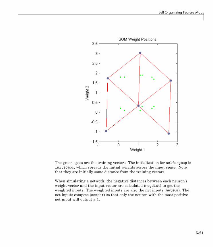
Self-Organizing Feature Maps
The green spots are the training vectors. The initialization for selforgmap isinitsompc, which spreads the initial weights across the input space. Notethat they are initially some distance from the training vectors.
When simulating a network, the negative distances between each neuron’sweight vector and the input vector are calculated (negdist) to get theweighted inputs. The weighted inputs are also the net inputs (netsum). Thenet inputs compete (compet) so that only the neuron with the most positivenet input will output a 1.
6-21
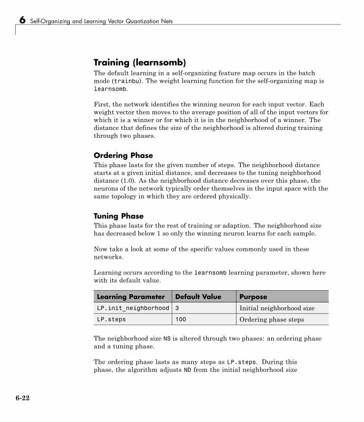
6 Self-Organizing and Learning Vector Quantization Nets
Training (learnsomb)The default learning in a self-organizing feature map occurs in the batchmode (trainbu). The weight learning function for the self-organizing map islearnsomb.
First, the network identifies the winning neuron for each input vector. Eachweight vector then moves to the average position of all of the input vectors forwhich it is a winner or for which it is in the neighborhood of a winner. Thedistance that defines the size of the neighborhood is altered during trainingthrough two phases.
Ordering PhaseThis phase lasts for the given number of steps. The neighborhood distancestarts at a given initial distance, and decreases to the tuning neighborhooddistance (1.0). As the neighborhood distance decreases over this phase, theneurons of the network typically order themselves in the input space with thesame topology in which they are ordered physically.
Tuning PhaseThis phase lasts for the rest of training or adaption. The neighborhood sizehas decreased below 1 so only the winning neuron learns for each sample.
Now take a look at some of the specific values commonly used in thesenetworks.
Learning occurs according to the learnsomb learning parameter, shown herewith its default value.
Learning Parameter Default Value Purpose
LP.init_neighborhood 3 Initial neighborhood size
LP.steps 100 Ordering phase steps
The neighborhood size NS is altered through two phases: an ordering phaseand a tuning phase.
The ordering phase lasts as many steps as LP.steps. During thisphase, the algorithm adjusts ND from the initial neighborhood size
6-22
Self-Organizing Feature Maps
LP.init_neighborhood down to 1. It is during this phase that neuronweights order themselves in the input space consistent with the associatedneuron positions.
During the tuning phase, ND is less than 1. During this phase, the weights areexpected to spread out relatively evenly over the input space while retainingtheir topological order found during the ordering phase.
Thus, the neuron’s weight vectors initially take large steps all togethertoward the area of input space where input vectors are occurring. Then as theneighborhood size decreases to 1, the map tends to order itself topologicallyover the presented input vectors. Once the neighborhood size is 1, the networkshould be fairly well ordered. The training continues in order to give theneurons time to spread out evenly across the input vectors.
As with competitive layers, the neurons of a self-organizing map will orderthemselves with approximately equal distances between them if input vectorsappear with even probability throughout a section of the input space. If inputvectors occur with varying frequency throughout the input space, the featuremap layer tends to allocate neurons to an area in proportion to the frequencyof input vectors there.
Thus, feature maps, while learning to categorize their input, also learn boththe topology and distribution of their input.
You can train the network for 1000 epochs with
net.trainParam.epochs = 1000;net = train(net,P);plotsompos(net,P);
6-23
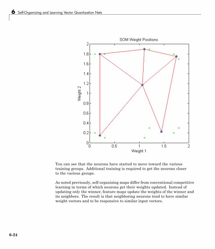
6 Self-Organizing and Learning Vector Quantization Nets
You can see that the neurons have started to move toward the varioustraining groups. Additional training is required to get the neurons closerto the various groups.
As noted previously, self-organizing maps differ from conventional competitivelearning in terms of which neurons get their weights updated. Instead ofupdating only the winner, feature maps update the weights of the winner andits neighbors. The result is that neighboring neurons tend to have similarweight vectors and to be responsive to similar input vectors.
6-24
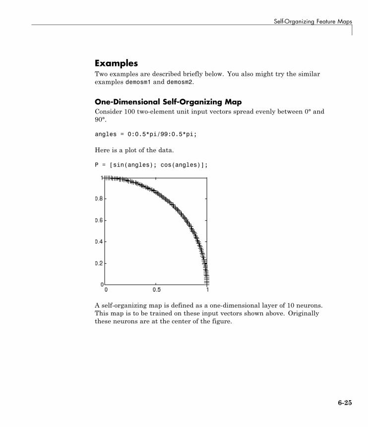
Self-Organizing Feature Maps
ExamplesTwo examples are described briefly below. You also might try the similarexamples demosm1 and demosm2.
One-Dimensional Self-Organizing MapConsider 100 two-element unit input vectors spread evenly between 0° and90°.
angles = 0:0.5*pi/99:0.5*pi;
Here is a plot of the data.
P = [sin(angles); cos(angles)];
A self-organizing map is defined as a one-dimensional layer of 10 neurons.This map is to be trained on these input vectors shown above. Originallythese neurons are at the center of the figure.
6-25
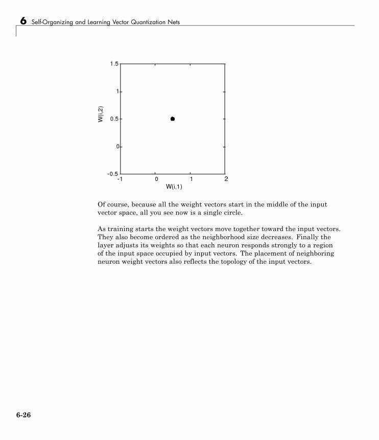
6 Self-Organizing and Learning Vector Quantization Nets
Of course, because all the weight vectors start in the middle of the inputvector space, all you see now is a single circle.
As training starts the weight vectors move together toward the input vectors.They also become ordered as the neighborhood size decreases. Finally thelayer adjusts its weights so that each neuron responds strongly to a regionof the input space occupied by input vectors. The placement of neighboringneuron weight vectors also reflects the topology of the input vectors.
6-26
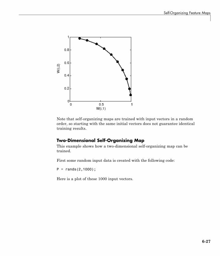
Self-Organizing Feature Maps
Note that self-organizing maps are trained with input vectors in a randomorder, so starting with the same initial vectors does not guarantee identicaltraining results.
Two-Dimensional Self-Organizing MapThis example shows how a two-dimensional self-organizing map can betrained.
First some random input data is created with the following code:
P = rands(2,1000);
Here is a plot of these 1000 input vectors.
6-27
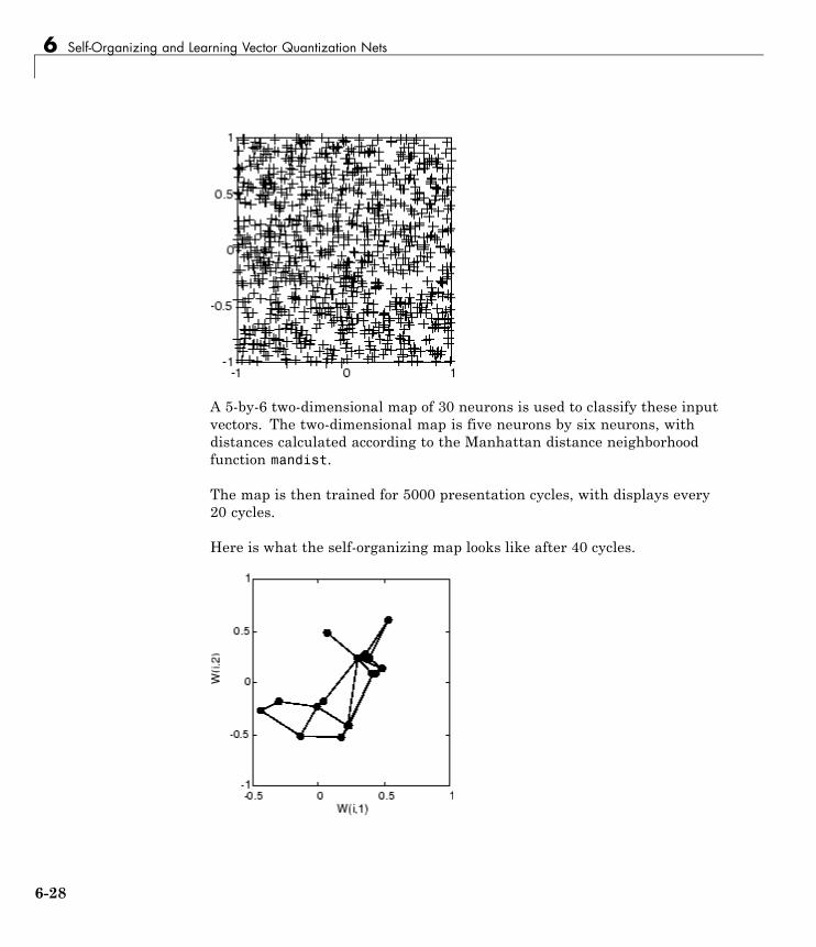
6 Self-Organizing and Learning Vector Quantization Nets
A 5-by-6 two-dimensional map of 30 neurons is used to classify these inputvectors. The two-dimensional map is five neurons by six neurons, withdistances calculated according to the Manhattan distance neighborhoodfunction mandist.
The map is then trained for 5000 presentation cycles, with displays every20 cycles.
Here is what the self-organizing map looks like after 40 cycles.
6-28
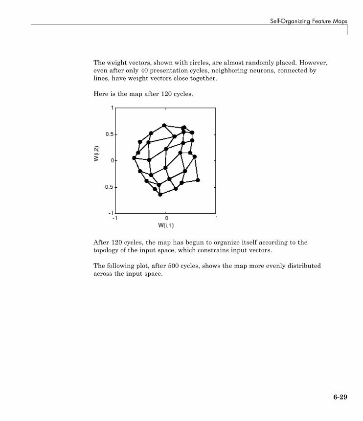
Self-Organizing Feature Maps
The weight vectors, shown with circles, are almost randomly placed. However,even after only 40 presentation cycles, neighboring neurons, connected bylines, have weight vectors close together.
Here is the map after 120 cycles.
After 120 cycles, the map has begun to organize itself according to thetopology of the input space, which constrains input vectors.
The following plot, after 500 cycles, shows the map more evenly distributedacross the input space.
6-29
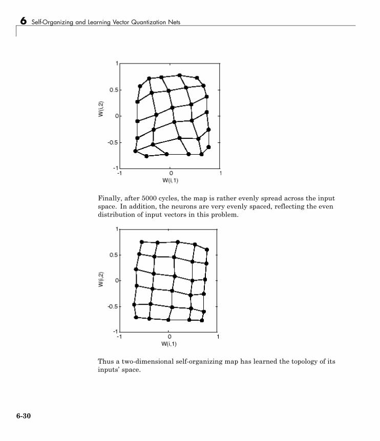
6 Self-Organizing and Learning Vector Quantization Nets
Finally, after 5000 cycles, the map is rather evenly spread across the inputspace. In addition, the neurons are very evenly spaced, reflecting the evendistribution of input vectors in this problem.
Thus a two-dimensional self-organizing map has learned the topology of itsinputs’ space.
6-30
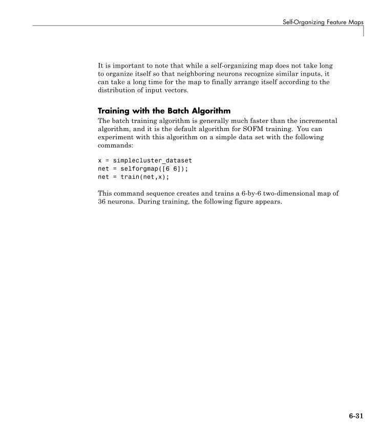
Self-Organizing Feature Maps
It is important to note that while a self-organizing map does not take longto organize itself so that neighboring neurons recognize similar inputs, itcan take a long time for the map to finally arrange itself according to thedistribution of input vectors.
Training with the Batch AlgorithmThe batch training algorithm is generally much faster than the incrementalalgorithm, and it is the default algorithm for SOFM training. You canexperiment with this algorithm on a simple data set with the followingcommands:
x = simplecluster_datasetnet = selforgmap([6 6]);net = train(net,x);
This command sequence creates and trains a 6-by-6 two-dimensional map of36 neurons. During training, the following figure appears.
6-31
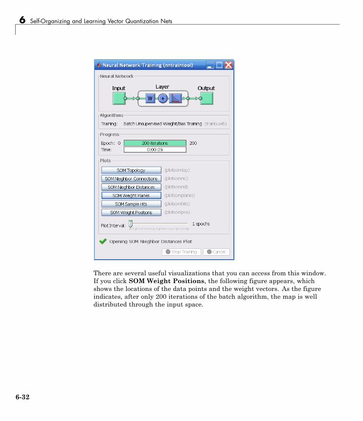
6 Self-Organizing and Learning Vector Quantization Nets
There are several useful visualizations that you can access from this window.If you click SOM Weight Positions, the following figure appears, whichshows the locations of the data points and the weight vectors. As the figureindicates, after only 200 iterations of the batch algorithm, the map is welldistributed through the input space.
6-32
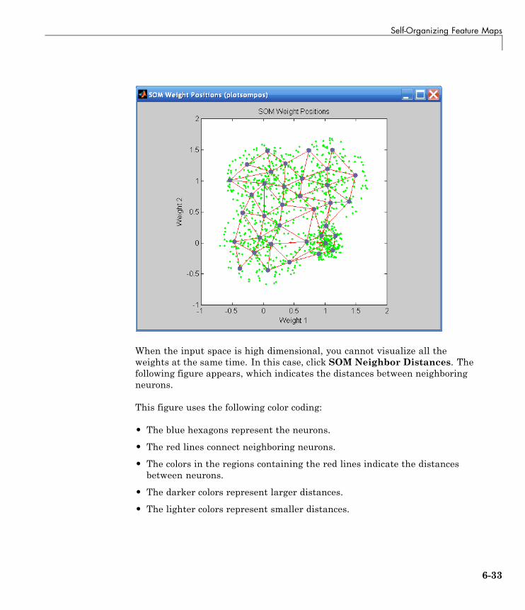
Self-Organizing Feature Maps
When the input space is high dimensional, you cannot visualize all theweights at the same time. In this case, click SOM Neighbor Distances. Thefollowing figure appears, which indicates the distances between neighboringneurons.
This figure uses the following color coding:
• The blue hexagons represent the neurons.
• The red lines connect neighboring neurons.
• The colors in the regions containing the red lines indicate the distancesbetween neurons.
• The darker colors represent larger distances.
• The lighter colors represent smaller distances.
6-33
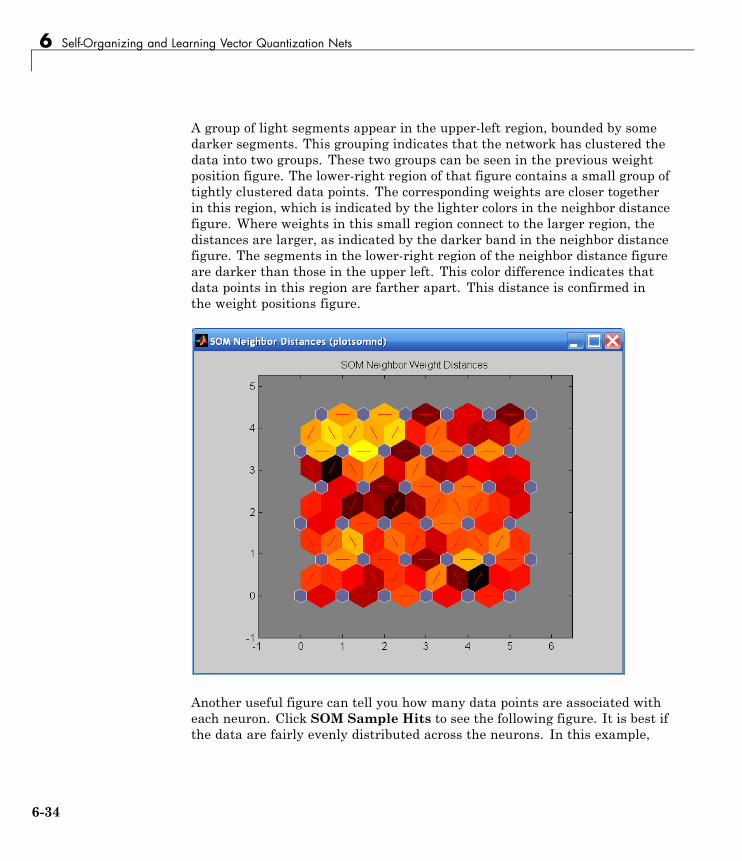
6 Self-Organizing and Learning Vector Quantization Nets
A group of light segments appear in the upper-left region, bounded by somedarker segments. This grouping indicates that the network has clustered thedata into two groups. These two groups can be seen in the previous weightposition figure. The lower-right region of that figure contains a small group oftightly clustered data points. The corresponding weights are closer togetherin this region, which is indicated by the lighter colors in the neighbor distancefigure. Where weights in this small region connect to the larger region, thedistances are larger, as indicated by the darker band in the neighbor distancefigure. The segments in the lower-right region of the neighbor distance figureare darker than those in the upper left. This color difference indicates thatdata points in this region are farther apart. This distance is confirmed inthe weight positions figure.
Another useful figure can tell you how many data points are associated witheach neuron. Click SOM Sample Hits to see the following figure. It is best ifthe data are fairly evenly distributed across the neurons. In this example,
6-34
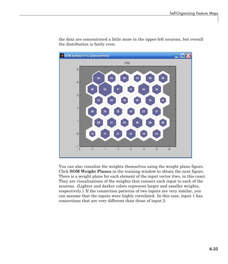
Self-Organizing Feature Maps
the data are concentrated a little more in the upper-left neurons, but overallthe distribution is fairly even.
You can also visualize the weights themselves using the weight plane figure.Click SOM Weight Planes in the training window to obtain the next figure.There is a weight plane for each element of the input vector (two, in this case).They are visualizations of the weights that connect each input to each of theneurons. (Lighter and darker colors represent larger and smaller weights,respectively.) If the connection patterns of two inputs are very similar, youcan assume that the inputs were highly correlated. In this case, input 1 hasconnections that are very different than those of input 2.
6-35
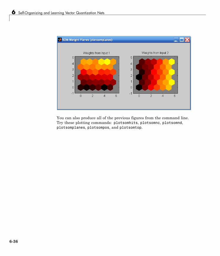
6 Self-Organizing and Learning Vector Quantization Nets
You can also produce all of the previous figures from the command line.Try these plotting commands: plotsomhits, plotsomnc, plotsomnd,plotsomplanes, plotsompos, and plotsomtop.
6-36
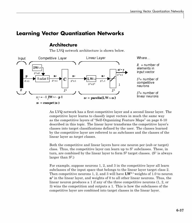
Learning Vector Quantization Networks
Learning Vector Quantization Networks
ArchitectureThe LVQ network architecture is shown below.
An LVQ network has a first competitive layer and a second linear layer. Thecompetitive layer learns to classify input vectors in much the same wayas the competitive layers of “Self-Organizing Feature Maps” on page 6-10described in this topic. The linear layer transforms the competitive layer’sclasses into target classifications defined by the user. The classes learnedby the competitive layer are referred to as subclasses and the classes of thelinear layer as target classes.
Both the competitive and linear layers have one neuron per (sub or target)class. Thus, the competitive layer can learn up to S1 subclasses. These, inturn, are combined by the linear layer to form S2 target classes. (S1 is alwayslarger than S2.)
For example, suppose neurons 1, 2, and 3 in the competitive layer all learnsubclasses of the input space that belongs to the linear layer target class 2.Then competitive neurons 1, 2, and 3 will have LW2,1 weights of 1.0 to neuronn2 in the linear layer, and weights of 0 to all other linear neurons. Thus, thelinear neuron produces a 1 if any of the three competitive neurons (1, 2, or3) wins the competition and outputs a 1. This is how the subclasses of thecompetitive layer are combined into target classes in the linear layer.
6-37
6 Self-Organizing and Learning Vector Quantization Nets
In short, a 1 in the ith row of a1 (the rest to the elements of a1 will be zero)effectively picks the ith column of LW2,1 as the network output. Each suchcolumn contains a single 1, corresponding to a specific class. Thus, subclass1s from layer 1 are put into various classes by the LW2,1a1 multiplication inlayer 2.
You know ahead of time what fraction of the layer 1 neurons should beclassified into the various class outputs of layer 2, so you can specify theelements of LW2,1 at the start. However, you have to go through a trainingprocedure to get the first layer to produce the correct subclass output for eachvector of the training set. This training is discussed in “Training” on page 6-6.First, consider how to create the original network.
Creating an LVQ NetworkYou can create an LVQ network with the function newlvq,
net = newlvq(PR,S1,PC,LR,LF)
where
• PR is an R-by-2 matrix of minimum and maximum values for R inputelements.
• S1 is the number of first-layer hidden neurons.
• PC is an S2-element vector of typical class percentages.
• LR is the learning rate (default 0.01).
• LF is the learning function (default is learnlv1).
Suppose you have 10 input vectors. Create a network that assigns each ofthese input vectors to one of four subclasses. Thus, there are four neurons inthe first competitive layer. These subclasses are then assigned to one of twooutput classes by the two neurons in layer 2. The input vectors and targetsare specified by
P = [-3 -2 -2 0 0 0 0 2 2 3; 0 1 -1 2 1 -1 -2 1 -1 0];
and
Tc = [1 1 1 2 2 2 2 1 1 1];
6-38
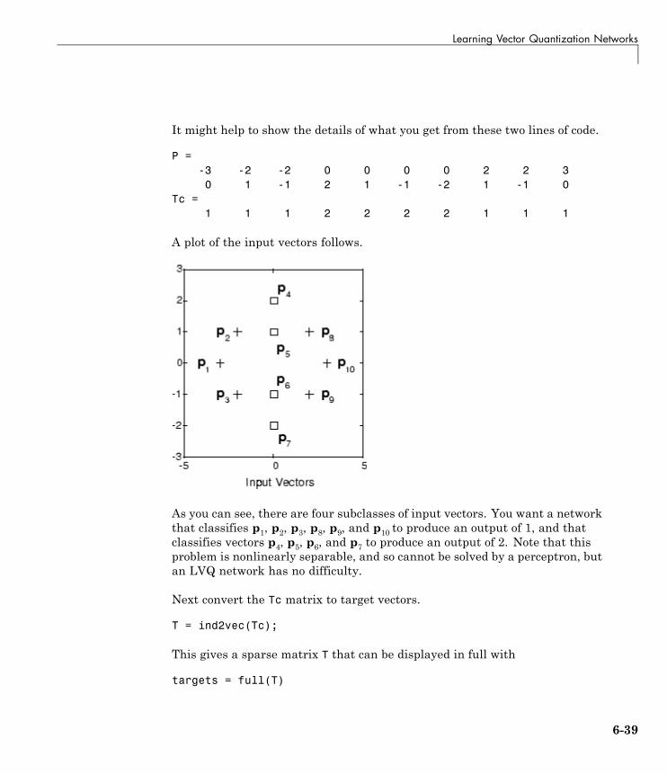
Learning Vector Quantization Networks
It might help to show the details of what you get from these two lines of code.
P =-3 -2 -2 0 0 0 0 2 2 30 1 -1 2 1 -1 -2 1 -1 0
Tc =1 1 1 2 2 2 2 1 1 1
A plot of the input vectors follows.
As you can see, there are four subclasses of input vectors. You want a networkthat classifies p1, p2, p3, p8, p9, and p10 to produce an output of 1, and thatclassifies vectors p4, p5, p6, and p7 to produce an output of 2. Note that thisproblem is nonlinearly separable, and so cannot be solved by a perceptron, butan LVQ network has no difficulty.
Next convert the Tc matrix to target vectors.
T = ind2vec(Tc);
This gives a sparse matrix T that can be displayed in full with
targets = full(T)
6-39
6 Self-Organizing and Learning Vector Quantization Nets
which gives
targets =1 1 1 0 0 0 0 1 1 10 0 0 1 1 1 1 0 0 0
This looks right. It says, for instance, that if you have the first column of Pas input, you should get the first column of targets as an output; and thatoutput says the input falls in class 1, which is correct. Now you are ready tocall newlvq.
Call newlvq with the proper arguments so that it creates a network with fourneurons in the first layer and two neurons in the second layer. The first-layerweights are initialized to the centers of the input ranges with the functionmidpoint. The second-layer weights have 60% (6 of the 10 in Tc above) of itscolumns with a 1 in the first row, (corresponding to class 1), and 40% of itscolumns will have a 1 in the second row (corresponding to class 2).
net = newlvq(P,4,[.6 .4]);
Confirm the initial values of the first-layer weight matrix.
net.IW{1,1}ans =
0 00 00 00 0
These zero weights are indeed the values at the midpoint of the ranges (−3 to+3) of the inputs, as you would expect when using midpoint for initialization.
You can look at the second-layer weights with
net.LW{2,1}ans =
1 1 0 00 0 1 1
6-40
Learning Vector Quantization Networks
This makes sense too. It says that if the competitive layer produces a 1 as thefirst or second element, the input vector is classified as class 1; otherwise itis a class 2.
You might notice that the first two competitive neurons are connected tothe first linear neuron (with weights of 1), while the second two competitiveneurons are connected to the second linear neuron. All other weights betweenthe competitive neurons and linear neurons have values of 0. Thus, eachof the two target classes (the linear neurons) is, in fact, the union of twosubclasses (the competitive neurons).
You can simulate the network with sim. Use the original P matrix as inputjust to see what you get.
Y = sim(net,P);Yc = vec2ind(Y)Yc =
1 1 1 1 1 1 1 1 1 1
The network classifies all inputs into class 1. Because this is not what youwant, you have to train the network (adjusting the weights of layer 1 only),before you can expect a good result. The next two sections discuss two LVQlearning rules and the training process.
LVQ1 Learning Rule (learnlv1)LVQ learning in the competitive layer is based on a set of input/target pairs.
p t p t p t1 1 2 2, , , , ,{ } { } { } Q Q
Each target vector has a single 1. The rest of its elements are 0. The 1 tellsthe proper classification of the associated input. For instance, consider thefollowing training pair.
p t1 1
21
0
0010
= −⎡
⎣
⎢⎢⎢
⎤
⎦
⎥⎥⎥
=
⎡
⎣
⎢⎢⎢⎢
⎤
⎦
⎥⎥⎥⎥
⎧
⎨⎪⎪
⎩⎪⎪
⎫
⎬⎪⎪
⎭⎪⎪
,
6-41
6 Self-Organizing and Learning Vector Quantization Nets
Here there are input vectors of three elements, and each input vector is tobe assigned to one of four classes. The network is to be trained so that itclassifies the input vector shown above into the third of four classes.
To train the network, an input vector p is presented, and the distance from pto each row of the input weight matrix IW1,1 is computed with the functionnegdist. The hidden neurons of layer 1 compete. Suppose that the ithelement of n1 is most positive, and neuron i* wins the competition. Thenthe competitive transfer function produces a 1 as the i*th element of a1. Allother elements of a1 are 0.
When a1 is multiplied by the layer 2 weights LW2,1, the single 1 in a1 selectsthe class k* associated with the input. Thus, the network has assigned theinput vector p to class k* and α2k* will be 1. Of course, this assignment can bea good one or a bad one, for tk* can be 1 or 0, depending on whether the inputbelonged to class k* or not.
Adjust the i*th row of IW1,1 in such a way as to move this row closer to theinput vector p if the assignment is correct, and to move the row away from pif the assignment is incorrect. If p is classified correctly,
k kt∗ ∗= =( )2 1
compute the new value of the i*th row of IW1,1 as
i i iq q q q∗ ∗ ∗= − + − −IW IW p IW1 1 1 1 1 11 1, , ,( ) ( ) ( ( ) ( ))
On the other hand, if p is classified incorrectly,
k kt∗ ∗= ≠ =( )2 1 0
compute the new value of the i*th row of IW1,1 as
i i iq q q q∗ ∗ ∗= − − − −IW IW p IW1 1 1 1 1 11 1, , ,( ) ( ) ( ( ) ( ))
6-42
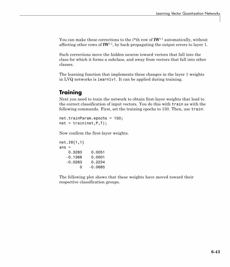
Learning Vector Quantization Networks
You can make these corrections to the i*th row of IW1,1 automatically, withoutaffecting other rows of IW1,1, by back-propagating the output errors to layer 1.
Such corrections move the hidden neuron toward vectors that fall into theclass for which it forms a subclass, and away from vectors that fall into otherclasses.
The learning function that implements these changes in the layer 1 weightsin LVQ networks is learnlv1. It can be applied during training.
TrainingNext you need to train the network to obtain first-layer weights that lead tothe correct classification of input vectors. You do this with train as with thefollowing commands. First, set the training epochs to 150. Then, use train:
net.trainParam.epochs = 150;net = train(net,P,T);
Now confirm the first-layer weights.
net.IW{1,1}ans =
0.3283 0.0051-0.1366 0.0001-0.0263 0.2234
0 -0.0685
The following plot shows that these weights have moved toward theirrespective classification groups.
6-43
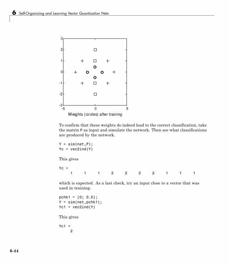
6 Self-Organizing and Learning Vector Quantization Nets
To confirm that these weights do indeed lead to the correct classification, takethe matrix P as input and simulate the network. Then see what classificationsare produced by the network.
Y = sim(net,P);Yc = vec2ind(Y)
This gives
Yc =1 1 1 2 2 2 2 1 1 1
which is expected. As a last check, try an input close to a vector that wasused in training.
pchk1 = [0; 0.5];Y = sim(net,pchk1);Yc1 = vec2ind(Y)
This gives
Yc1 =2
6-44
Learning Vector Quantization Networks
This looks right, because pchk1 is close to other vectors classified as 2.Similarly,
pchk2 = [1; 0];Y = sim(net,pchk2);Yc2 = vec2ind(Y)
gives
Yc2 =1
This looks right too, because pchk2 is close to other vectors classified as 1.
You might want to try the example program demolvq1. It follows thediscussion of training given above.
Supplemental LVQ2.1 Learning Rule (learnlv2)The following learning rule is one that might be applied after first applyingLVQ1. It can improve the result of the first learning. This particular versionof LVQ2 (referred to as LVQ2.1 in the literature [Koho97]) is embodied in thefunction learnlv2. Note again that LVQ2.1 is to be used only after LVQ1has been applied.
Learning here is similar to that in learnlv2 except now two vectors of layer 1that are closest to the input vector can be updated, provided that one belongsto the correct class and one belongs to a wrong class, and further providedthat the input falls into a “window” near the midplane of the two vectors.
The window is defined by
min ,dd
d
dsi
j
j
i
⎛
⎝⎜⎜
⎞
⎠⎟⎟ >
where
6-45
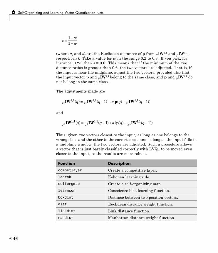
6 Self-Organizing and Learning Vector Quantization Nets
sww
≡ −+
11
(where di and dj are the Euclidean distances of p from i*IW1,1 and j*IW
1,1,respectively). Take a value for w in the range 0.2 to 0.3. If you pick, forinstance, 0.25, then s = 0.6. This means that if the minimum of the twodistance ratios is greater than 0.6, the two vectors are adjusted. That is, ifthe input is near the midplane, adjust the two vectors, provided also thatthe input vector p and j*IW
1,1 belong to the same class, and p and i*IW1,1 do
not belong in the same class.
The adjustments made are
i i iq q q q∗ ∗ ∗= − − − −IW IW p IW1 1 1 1 1 11 1, , ,( ) ( ) ( ( ) ( ))
and
j j jq q q q∗ ∗ ∗= − + − −IW IW p IW1 1 1 1 1 11 1, , ,( ) ( ) ( ( ) ( ))
Thus, given two vectors closest to the input, as long as one belongs to thewrong class and the other to the correct class, and as long as the input falls ina midplane window, the two vectors are adjusted. Such a procedure allowsa vector that is just barely classified correctly with LVQ1 to be moved evencloser to the input, so the results are more robust.
Function Description
competlayer Create a competitive layer.
learnk Kohonen learning rule.
selforgmap Create a self-organizing map.
learncon Conscience bias learning function.
boxdist Distance between two position vectors.
dist Euclidean distance weight function.
linkdist Link distance function.
mandist Manhattan distance weight function.
6-46
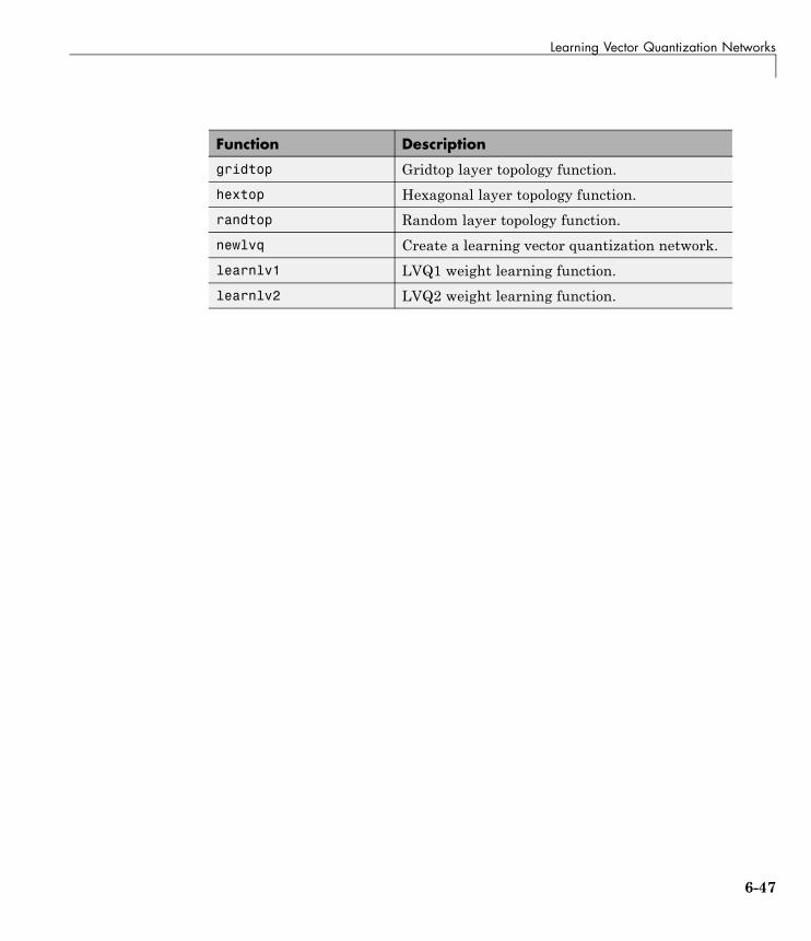
Learning Vector Quantization Networks
Function Description
gridtop Gridtop layer topology function.
hextop Hexagonal layer topology function.
randtop Random layer topology function.
newlvq Create a learning vector quantization network.
learnlv1 LVQ1 weight learning function.
learnlv2 LVQ2 weight learning function.
6-47

6 Self-Organizing and Learning Vector Quantization Nets
6-48

7
Adaptive Filters andAdaptive Training
• “Introduction” on page 7-2
• “Linear Neuron Model” on page 7-3
• “Adaptive Linear Network Architecture” on page 7-4
• “Least Mean Square Error” on page 7-8
• “LMS Algorithm (learnwh)” on page 7-9
• “Adaptive Filtering (adapt)” on page 7-10
7 Adaptive Filters and Adaptive Training
IntroductionThe ADALINE (adaptive linear neuron) networks discussed in this chapterare similar to the perceptron, but their transfer function is linear rather thanhard-limiting. This allows their outputs to take on any value, whereas theperceptron output is limited to either 0 or 1. Both the ADALINE and theperceptron can only solve linearly separable problems. However, here theLMS (least mean squares) learning rule, which is much more powerful thanthe perceptron learning rule, is used. The LMS, or Widrow-Hoff, learning ruleminimizes the mean square error and thus moves the decision boundaries asfar as it can from the training patterns.
In this chapter, you design an adaptive linear system that responds to changesin its environment as it is operating. Linear networks that are adjusted ateach time step based on new input and target vectors can find weights andbiases that minimize the network’s sum-squared error for recent input andtarget vectors. Networks of this sort are often used in error cancelation, signalprocessing, and control systems.
The pioneering work in this field was done by Widrow and Hoff, who gave thename ADALINE to adaptive linear elements. The basic reference on thissubject is Widrow, B., and S.D. Sterns, Adaptive Signal Processing, New York,Prentice-Hall, 1985.
The adaptive training of self-organizing and competitive networks is alsoconsidered in this chapter.
Important Adaptive FunctionsThis chapter introduces the function adapt, which changes the weights andbiases of a network incrementally during training.
You can type help linnet to see a list of linear and adaptive networkfunctions, examples, and applications.
7-2
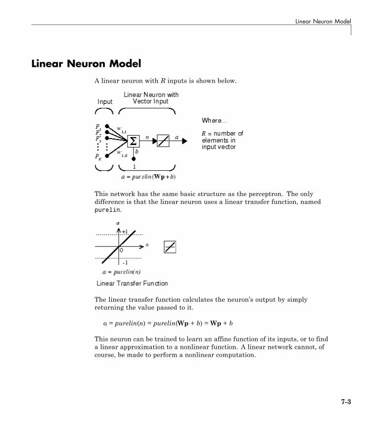
Linear Neuron Model
Linear Neuron ModelA linear neuron with R inputs is shown below.
This network has the same basic structure as the perceptron. The onlydifference is that the linear neuron uses a linear transfer function, namedpurelin.
The linear transfer function calculates the neuron’s output by simplyreturning the value passed to it.
α = purelin(n) = purelin(Wp + b) = Wp + b
This neuron can be trained to learn an affine function of its inputs, or to finda linear approximation to a nonlinear function. A linear network cannot, ofcourse, be made to perform a nonlinear computation.
7-3
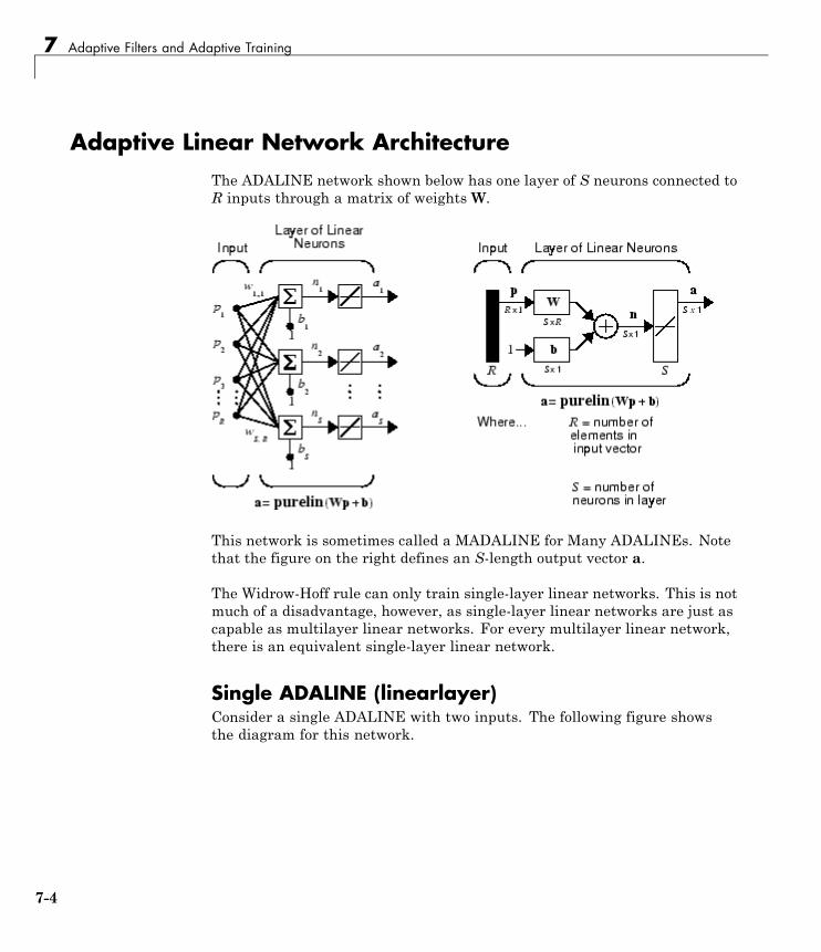
7 Adaptive Filters and Adaptive Training
Adaptive Linear Network ArchitectureThe ADALINE network shown below has one layer of S neurons connected toR inputs through a matrix of weights W.
This network is sometimes called a MADALINE for Many ADALINEs. Notethat the figure on the right defines an S-length output vector a.
The Widrow-Hoff rule can only train single-layer linear networks. This is notmuch of a disadvantage, however, as single-layer linear networks are just ascapable as multilayer linear networks. For every multilayer linear network,there is an equivalent single-layer linear network.
Single ADALINE (linearlayer)Consider a single ADALINE with two inputs. The following figure showsthe diagram for this network.
7-4
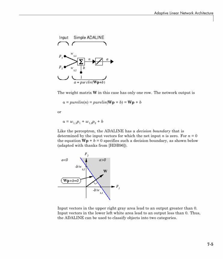
Adaptive Linear Network Architecture
The weight matrixW in this case has only one row. The network output is
α = purelin(n) = purelin(Wp + b) = Wp + b
or
α = w1,1p1 + w1,2p2 + b
Like the perceptron, the ADALINE has a decision boundary that isdetermined by the input vectors for which the net input n is zero. For n = 0the equation Wp + b = 0 specifies such a decision boundary, as shown below(adapted with thanks from [HDB96]).
Input vectors in the upper right gray area lead to an output greater than 0.Input vectors in the lower left white area lead to an output less than 0. Thus,the ADALINE can be used to classify objects into two categories.
7-5
7 Adaptive Filters and Adaptive Training
However, ADALINE can classify objects in this way only when the objectsare linearly separable. Thus, ADALINE has the same limitation as theperceptron.
You can create a network similar to the one shown using this command:
net = linearlayer;net = configure(net,[0;0],[0]);
The sizes of the two arguments to configure indicate that the layer is to havetwo inputs and one output. Normally train does this configuration for you,but this allows us to inspect the weights before training.
The network weights and biases are set to zero, by default. You can see thecurrent values using the commands:
W = net.IW{1,1}W =
0 0
and
b = net.b{1}b =
0
You can also assign arbitrary values to the weights and bias, such as 2 and 3for the weights and −4 for the bias:
net.IW{1,1} = [2 3];net.b{1} = -4;
You can simulate the ADAPLINE for a particular input vector.
p = [5; 6];a = sim(net,p)a =
24
7-6

Adaptive Linear Network Architecture
To summarize, you can create an ADALINE network with newlin, adjust itselements as you want, and simulate it with sim. You can find more aboutnewlin by typing help newlin.
7-7
7 Adaptive Filters and Adaptive Training
Least Mean Square ErrorLike the perceptron learning rule, the least mean square error (LMS)algorithm is an example of supervised training, in which the learning rule isprovided with a set of examples of desired network behavior.
p t p t p t1 1 2 2, , , , ,{ } { } { } Q Q
Here pq is an input to the network, and tq is the corresponding target output.As each input is applied to the network, the network output is comparedto the target. The error is calculated as the difference between the targetoutput and the network output. The goal is to minimize the average of thesum of these errors.
mseQ
e kQ
t k kk
Q
k
Q= = −
= =∑ ∑1 12
1
2
1
( ) ( ) ( ))
The LMS algorithm adjusts the weights and biases of the ADALINE so asto minimize this mean square error.
Fortunately, the mean square error performance index for the ADALINEnetwork is a quadratic function. Thus, the performance index will either haveone global minimum, a weak minimum, or no minimum, depending on thecharacteristics of the input vectors. Specifically, the characteristics of theinput vectors determine whether or not a unique solution exists.
You can learn more about this topic in Chapter 10 of [HDB96].
7-8
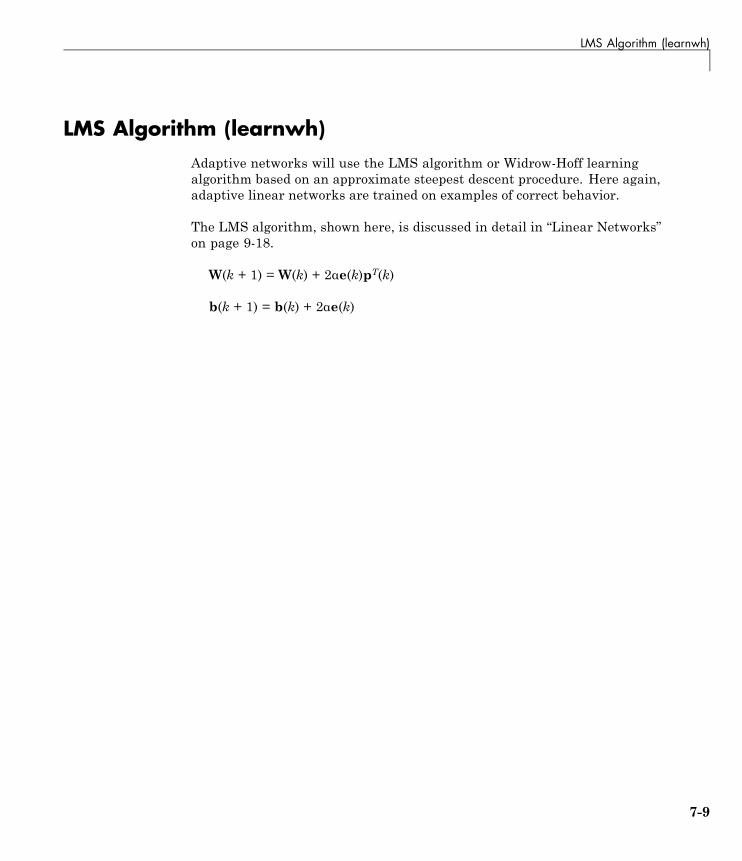
LMS Algorithm (learnwh)
LMS Algorithm (learnwh)Adaptive networks will use the LMS algorithm or Widrow-Hoff learningalgorithm based on an approximate steepest descent procedure. Here again,adaptive linear networks are trained on examples of correct behavior.
The LMS algorithm, shown here, is discussed in detail in “Linear Networks”on page 9-18.
W(k + 1) = W(k) + 2αe(k)pT(k)
b(k + 1) = b(k) + 2αe(k)
7-9
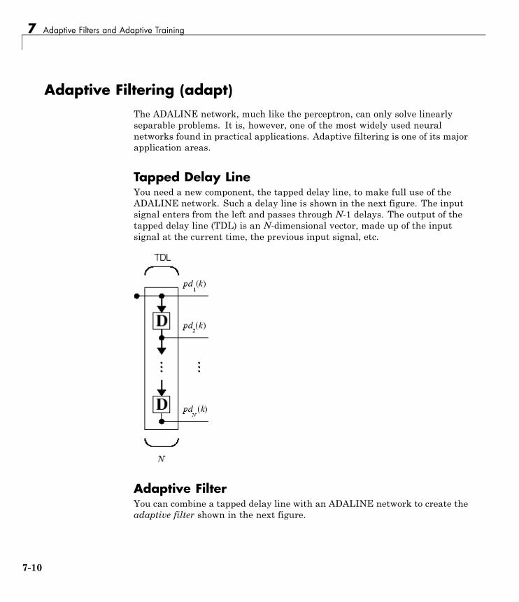
7 Adaptive Filters and Adaptive Training
Adaptive Filtering (adapt)The ADALINE network, much like the perceptron, can only solve linearlyseparable problems. It is, however, one of the most widely used neuralnetworks found in practical applications. Adaptive filtering is one of its majorapplication areas.
Tapped Delay LineYou need a new component, the tapped delay line, to make full use of theADALINE network. Such a delay line is shown in the next figure. The inputsignal enters from the left and passes through N-1 delays. The output of thetapped delay line (TDL) is an N-dimensional vector, made up of the inputsignal at the current time, the previous input signal, etc.
Adaptive FilterYou can combine a tapped delay line with an ADALINE network to create theadaptive filter shown in the next figure.
7-10
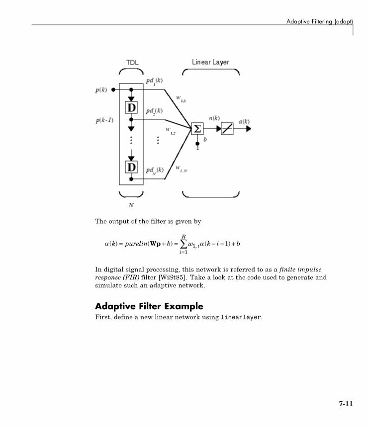
Adaptive Filtering (adapt)
The output of the filter is given by
( ) ( ) ( ),k purelin b w k i bii
R= + = − + +
=∑Wp 1
1
1
In digital signal processing, this network is referred to as a finite impulseresponse (FIR) filter [WiSt85]. Take a look at the code used to generate andsimulate such an adaptive network.
Adaptive Filter ExampleFirst, define a new linear network using linearlayer.
7-11
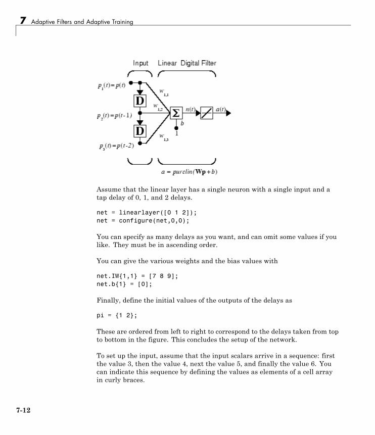
7 Adaptive Filters and Adaptive Training
Assume that the linear layer has a single neuron with a single input and atap delay of 0, 1, and 2 delays.
net = linearlayer([0 1 2]);net = configure(net,0,0);
You can specify as many delays as you want, and can omit some values if youlike. They must be in ascending order.
You can give the various weights and the bias values with
net.IW{1,1} = [7 8 9];net.b{1} = [0];
Finally, define the initial values of the outputs of the delays as
pi = {1 2};
These are ordered from left to right to correspond to the delays taken from topto bottom in the figure. This concludes the setup of the network.
To set up the input, assume that the input scalars arrive in a sequence: firstthe value 3, then the value 4, next the value 5, and finally the value 6. Youcan indicate this sequence by defining the values as elements of a cell arrayin curly braces.
7-12
Adaptive Filtering (adapt)
p = {3 4 5 6};
Now, you have a network and a sequence of inputs. Simulate the network tosee what its output is as a function of time.
[a,pf] = sim(net,p,pi)
This simulation yields an output sequence
a[46] [70] [94] [118]
and final values for the delay outputs of
pf[5] [6]
The example is sufficiently simple that you can check it without a calculatorto make sure that you understand the inputs, initial values of the delays, etc.
The network just defined can be trained with the function adapt to producea particular output sequence. Suppose, for instance, you want the networkto produce the sequence of values 10, 20, 30, 40.
t = {10 20 30 40};
You can train the defined network to do this, starting from the initial delayconditions used above. Specify 10 passes through the input sequence with
net.adaptParam.passes = 10;
Then let the network adapt for 10 passes over the data.
for i=1:10[net,y,E,pf,af] = adapt(net,p,t,pi);
end
This code returns the final weights, bias, and output sequence shown here.
wts = net.IW{1,1}wts =
7-13
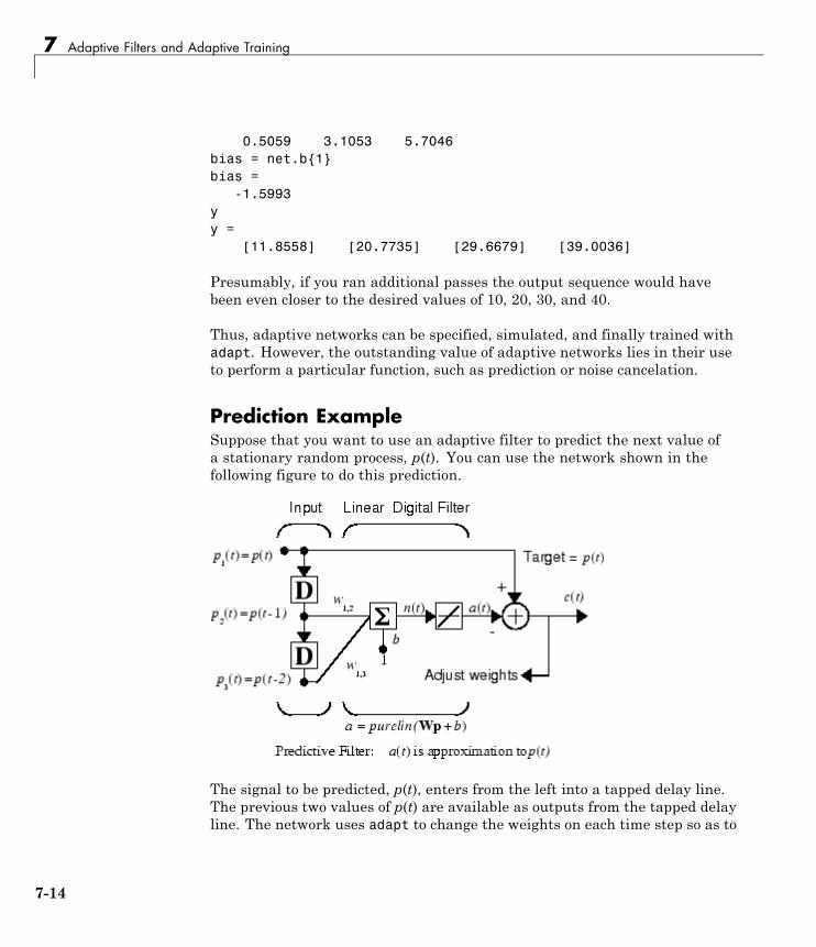
7 Adaptive Filters and Adaptive Training
0.5059 3.1053 5.7046bias = net.b{1}bias =
-1.5993yy =
[11.8558] [20.7735] [29.6679] [39.0036]
Presumably, if you ran additional passes the output sequence would havebeen even closer to the desired values of 10, 20, 30, and 40.
Thus, adaptive networks can be specified, simulated, and finally trained withadapt. However, the outstanding value of adaptive networks lies in their useto perform a particular function, such as prediction or noise cancelation.
Prediction ExampleSuppose that you want to use an adaptive filter to predict the next value ofa stationary random process, p(t). You can use the network shown in thefollowing figure to do this prediction.
The signal to be predicted, p(t), enters from the left into a tapped delay line.The previous two values of p(t) are available as outputs from the tapped delayline. The network uses adapt to change the weights on each time step so as to
7-14
Adaptive Filtering (adapt)
minimize the error e(t) on the far right. If this error is 0, the network outputa(t) is exactly equal to p(t), and the network has done its prediction properly.
Given the autocorrelation function of the stationary random process p(t),you can calculate the error surface, the maximum learning rate, and theoptimum values of the weights. Commonly, of course, you do not havedetailed information about the random process, so these calculations cannotbe performed. This lack does not matter to the network. After it is initializedand operating, the network adapts at each time step to minimize the errorand in a relatively short time is able to predict the input p(t).
Chapter 10 of [HDB96] presents this problem, goes through the analysis, andshows the weight trajectory during training. The network finds the optimumweights on its own without any difficulty whatsoever.
You also can try the example nnd10nc to see an adaptive noise cancelationprogram example in action. This example allows you to pick a learning rateand momentum (see “Multilayer Networks and Backpropagation Training” onpage 2-2), and shows the learning trajectory, and the original and cancelationsignals versus time.
Noise Cancelation ExampleConsider a pilot in an airplane. When the pilot speaks into a microphone, theengine noise in the cockpit combines with the voice signal. This additionalnoise makes the resultant signal heard by passengers of low quality. The goalis to obtain a signal that contains the pilot’s voice, but not the engine noise.You can cancel the noise with an adaptive filter if you obtain a sample of theengine noise and apply it as the input to the adaptive filter.
7-15
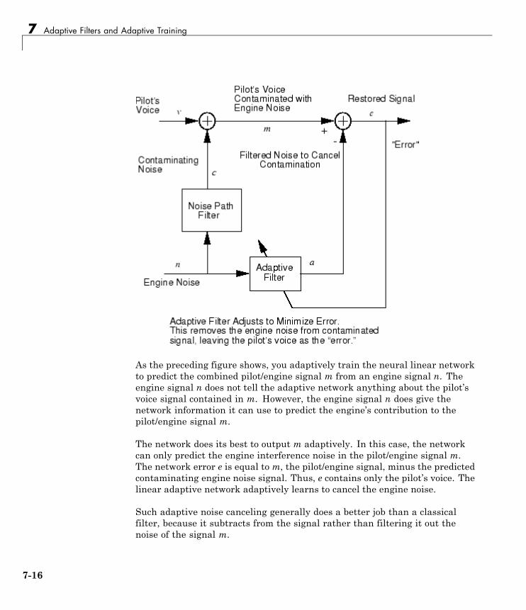
7 Adaptive Filters and Adaptive Training
As the preceding figure shows, you adaptively train the neural linear networkto predict the combined pilot/engine signal m from an engine signal n. Theengine signal n does not tell the adaptive network anything about the pilot’svoice signal contained in m. However, the engine signal n does give thenetwork information it can use to predict the engine’s contribution to thepilot/engine signal m.
The network does its best to output m adaptively. In this case, the networkcan only predict the engine interference noise in the pilot/engine signal m.The network error e is equal to m, the pilot/engine signal, minus the predictedcontaminating engine noise signal. Thus, e contains only the pilot’s voice. Thelinear adaptive network adaptively learns to cancel the engine noise.
Such adaptive noise canceling generally does a better job than a classicalfilter, because it subtracts from the signal rather than filtering it out thenoise of the signal m.
7-16
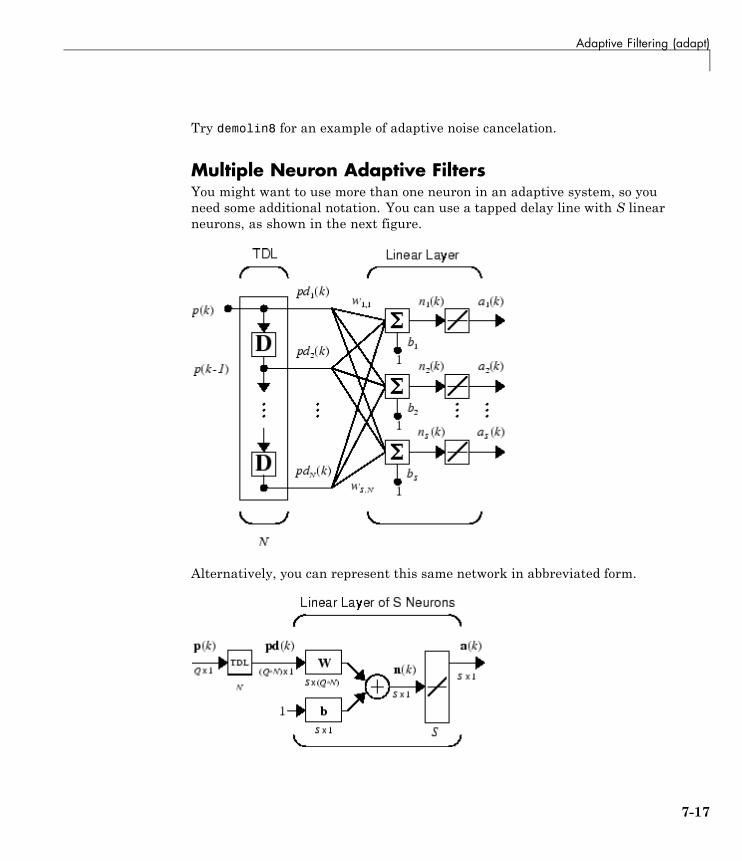
Adaptive Filtering (adapt)
Try demolin8 for an example of adaptive noise cancelation.
Multiple Neuron Adaptive FiltersYou might want to use more than one neuron in an adaptive system, so youneed some additional notation. You can use a tapped delay line with S linearneurons, as shown in the next figure.
Alternatively, you can represent this same network in abbreviated form.
7-17
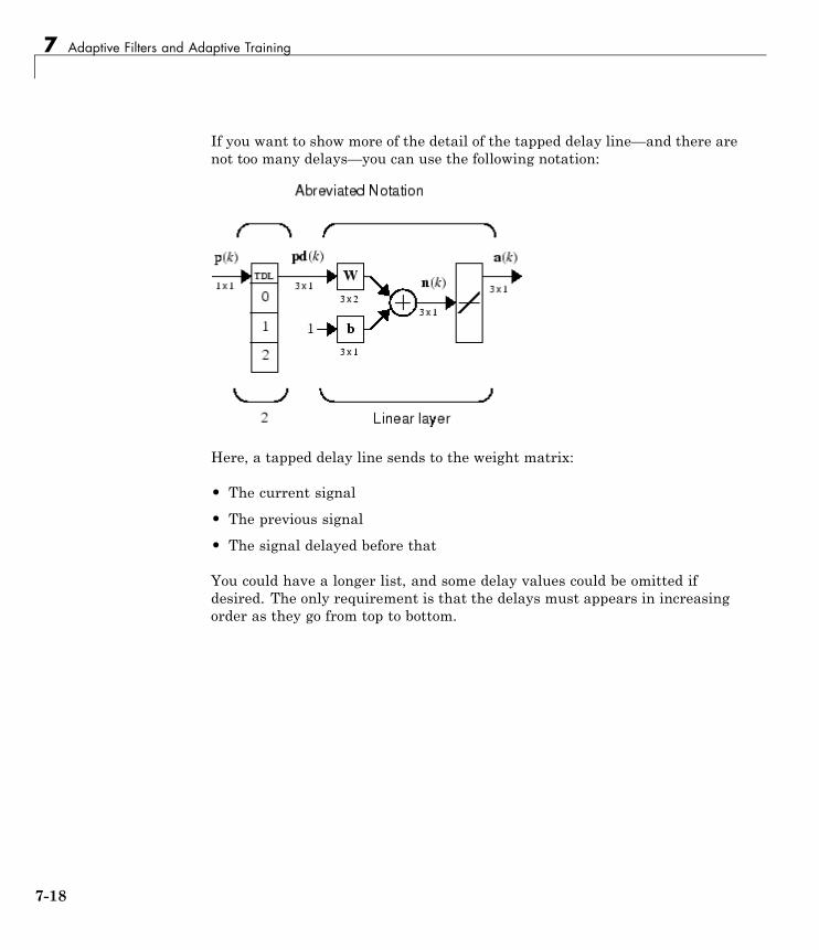
7 Adaptive Filters and Adaptive Training
If you want to show more of the detail of the tapped delay line—and there arenot too many delays—you can use the following notation:
Here, a tapped delay line sends to the weight matrix:
• The current signal
• The previous signal
• The signal delayed before that
You could have a longer list, and some delay values could be omitted ifdesired. The only requirement is that the delays must appears in increasingorder as they go from top to bottom.
7-18

8
Advanced Topics
• “Parallel and GPU Computing” on page 8-2
• “Speed and Memory Optimizations” on page 8-14
• “Multilayer Training Speed and Memory” on page 8-17
• “Improving Generalization” on page 8-34
• “Custom Networks” on page 8-46
• “Additional Toolbox Functions” on page 8-60
• “Custom Functions” on page 8-61
8 Advanced Topics
Parallel and GPU Computing
In this section...
“Modes of Parallelism” on page 8-2
“Distributed Computing” on page 8-3
“Single GPU Computing” on page 8-6
“Distributed GPU Computing” on page 8-9
“Parallel Time Series” on page 8-11
“Parallel Availability, Fallbacks, and Feedback” on page 8-11
Modes of ParallelismNeural networks are inherently very parallel algorithms. This parallelismcan be taken advantage of by multicore CPUs, graphical processing units(GPUs), and clusters of computers with multiple CPUs and GPUs.
Parallel Computing Toolbox™, when used in conjunction with NeuralNetwork Toolbox, allows neural network training and simulation to takeadvantage of each mode of parallelism.
Here is a standard single-threaded training and simulation session:
[x,t] = house_dataset;net1 = feedforwardnet(10);net2 = train(net1,x,t);y = net2(x);
The two steps that can be parallelized in this session are the call to train andthe implicit call to sim (where the network net2 is called as a function).
The form that parallelism in Neural Network Toolbox takes is that any data,such as x and t in the previous code, can be divided across samples. If x and tcontain only one sample each, there is no parallelism. But if x and t containhundreds or thousands of samples, parallelism can provide both speed andproblem size benefits.
8-2
Parallel and GPU Computing
Distributed ComputingParallel Computing Toolbox allows neural network training and simulation torun across multiple CPU cores on a single PC, or across multiple CPUs onmultiple computers on a network using MATLAB Distributed ComputingServer™.
Using multiple cores can speed up calculations. Using multiple computers canallow problems to be solved using datasets far too big to fit within the RAM ofany single computer. The only limit to problem size is the total quantity ofRAM available across all computers.
To manage cluster configurations, open the Cluster Profile Manager from theMATLAB Home tab Environment menu Parallel > Manage ClusterProfiles.
To open a pool of MATLAB workers using the default cluster profile, which isusually the local CPU cores, enter this command:
matlabpool open
Starting matlabpool using the 'local' profile ... connected to 4 labs.
When matlabpool open runs, it displays the number of workers available inthe pool. Another way to determine the number of workers is to query the pool:
poolSize = matlabpool('size')
poolSize =
4
Now the neural network can be trained and simulated with data splitby sample across all the workers. Do this by setting the train and simparameter 'useParallel' to 'yes'.
net2 = train(net1,x,t,'useParallel','yes')y = net2(x,'useParallel','yes')
Use the 'showResources' option to verify that the calculations really didrun across multiple workers.
8-3
8 Advanced Topics
net2 = train(net1,x,t,'useParallel','yes','showResources','yes')y = net2(x,'useParallel','yes','showResources','yes')
On a typical system, each line of code prints something like this:
Computing Resources:Parallel Workers
Worker 1 on MyComputer, MEX on PCWIN64Worker 2 on MyComputer, MEX on PCWIN64Worker 3 on MyComputer, MEX on PCWIN64Worker 4 on MyComputer, MEX on PCWIN64
When train and sim are called, the matrix or cell array data providedas input arguments are divided into distributed Composite values beforetraining and simulation. When sim has calculated a Composite output, it isconverted back to the same matrix or cell array form before being returned.
However, you might want to perform this data division manually for at leasttwo reasons. If the problem size is too large for the host computer, manuallydefining the elements of Composite values sequentially allows much biggerproblems to be defined.
Also, if it is known that some workers are on computers that are faster orhave more memory than others, you might want to distribute the data withdiffering numbers of samples per worker. This is called load balancing.
The following code sequentially creates a series of random datasets and savesthem to separate files:
for i=1:matlabpool('size')x = rand(2,1000);save(['inputs' num2str(i)],'x');t = x(1,:) .* x(2,:) + 2 * (x(1,:) + x(2,:));save(['targets' num2str(i)],'t');clear x t
end
Note that because the data was defined sequentially, it would be possible todefine a total dataset larger than could fit in the host PC memory. Only eachsub-dataset needs to be able to fit into memory at one time.
8-4
Parallel and GPU Computing
Now you can load the datasets sequentially across parallel workers, andtrain and simulate a network on the Composite data. When train or sim iscalled with Composite data, the 'useParallel' option is automatically set to'yes'. When using Composite data, the network’s input and outputs mustbe configured to match one of the datasets manually with the configurefunction before training.
xc = Composite;tc = Composite;for i=1:matlabpool('size')
data = load(['inputs' num2str(i)],'x');xc{i} = data.x;data = load(['targets' num2str(i)],'t');tc{i} = data.t;clear data
endnet2 = configure(net2,xc{1},tc{1});net2 = train(net2,xc,tc);yc = net2(xc);
To convert the Composite output returned by sim, you can access each of itselements, separately if concerned about memory limitations.
for i=1:matlabpool('size')yi = yc{i}
end
Or combined the Composite value into one local value if you are not concernedabout memory limitations.
y = {yc{:}};
When load balancing, the same process happens, but, instead of each datasethaving the same number of samples (1000 in the previous example), thenumbers of samples can be adjusted to best take advantage of the memoryand speed differences of the worker host computers.
It is not required that each worker have data. If element i of a Compositevalue is undefined, worker i will not be used in the computation.
8-5
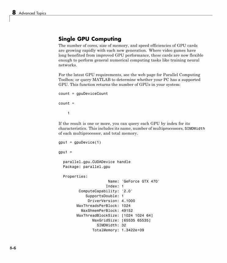
8 Advanced Topics
Single GPU ComputingThe number of cores, size of memory, and speed efficiencies of GPU cardsare growing rapidly with each new generation. Where video games havelong benefited from improved GPU performance, these cards are now flexibleenough to perform general numerical computing tasks like training neuralnetworks.
For the latest GPU requirements, see the web page for Parallel ComputingToolbox; or query MATLAB to determine whether your PC has a supportedGPU. This function returns the number of GPUs in your system:
count = gpuDeviceCount
count =
1
If the result is one or more, you can query each GPU by index for itscharacteristics. This includes its name, number of multiprocessors, SIMDWidthof each multiprocessor, and total memory.
gpu1 = gpuDevice(1)
gpu1 =
parallel.gpu.CUDADevice handlePackage: parallel.gpu
Properties:Name: 'GeForce GTX 470'
Index: 1ComputeCapability: '2.0'
SupportsDouble: 1DriverVersion: 4.1000
MaxThreadsPerBlock: 1024MaxShmemPerBlock: 49152
MaxThreadBlockSize: [1024 1024 64]MaxGridSize: [65535 65535]
SIMDWidth: 32TotalMemory: 1.3422e+09
8-6
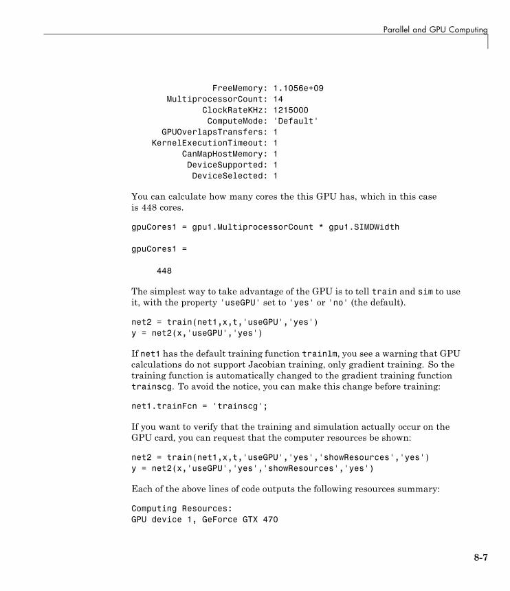
Parallel and GPU Computing
FreeMemory: 1.1056e+09MultiprocessorCount: 14
ClockRateKHz: 1215000ComputeMode: 'Default'
GPUOverlapsTransfers: 1KernelExecutionTimeout: 1
CanMapHostMemory: 1DeviceSupported: 1DeviceSelected: 1
You can calculate how many cores the this GPU has, which in this caseis 448 cores.
gpuCores1 = gpu1.MultiprocessorCount * gpu1.SIMDWidth
gpuCores1 =
448
The simplest way to take advantage of the GPU is to tell train and sim to useit, with the property 'useGPU' set to 'yes' or 'no' (the default).
net2 = train(net1,x,t,'useGPU','yes')y = net2(x,'useGPU','yes')
If net1 has the default training function trainlm, you see a warning that GPUcalculations do not support Jacobian training, only gradient training. So thetraining function is automatically changed to the gradient training functiontrainscg. To avoid the notice, you can make this change before training:
net1.trainFcn = 'trainscg';
If you want to verify that the training and simulation actually occur on theGPU card, you can request that the computer resources be shown:
net2 = train(net1,x,t,'useGPU','yes','showResources','yes')y = net2(x,'useGPU','yes','showResources','yes')
Each of the above lines of code outputs the following resources summary:
Computing Resources:GPU device 1, GeForce GTX 470
8-7
8 Advanced Topics
When a GPU is used in the previous examples, train and sim take MATLABmatrices or cell arrays and convert them to GPU arrays before training andsimulation. sim then takes the GPU array result and converts it back to amatrix or cell array before returning it.
An alternative is to supply the data arguments as values already converted toGPU arrays. The Parallel Computing Toolbox command for creating a GPUarray from a matrix is named accordingly.
xg = gpuArray(x)
To get the value back from the GPU use gather.
x2 = gather(xg)
However, for neural network calculations on a GPU to be efficient, matricesneed to be transposed and the columns padded so that the first element ineach column aligneds properly in the GPU memory. Do this with the functionnndata2gpu.
xg = nndata2gpu(x);tg = nndata2gpu(t);
Now you can train, simulate the network, and convert the returned GPU arrayback to MATLAB with the complement function gpu2nndata. When trainingwith gpuArray data, the network’s input and outputs must be configuredmanually with regular matrices using the configure function before training.
net2 = configure(net1,x,t);net2 = train(net2,xg,tg);yg = net2(xg);y = gpu2nndata(yg);
On GPUs and other hardware where you might want to deploy your neuralnetworks, it is often the case that the exponential function exp is notimplemented with hardware, but with a software library. This can slowdown neural networks that use the tansig sigmoid transfer function. Analternative function is the Elliot sigmoid function whose expression does notinclude a call to any higher order functions:
(equation) a = n / (1 + abs(n))
8-8
Parallel and GPU Computing
Before training, the network’s tansig layers can be converted to elliotsiglayers as follows:
for i=1:net.numLayersif strcmp(net.layers{i}.transferFcn,'tansig')
net.layers{i}.transferFcn = 'elliotsig';end
end
Now training and simulation might be faster on the GPU and simplerdeployment hardware.
Distributed GPU ComputingDistributed and GPU computing can be combined to run calculations acrossmultiple GPUs and/or CPUs on a single PC or clusters of PCs with MATLABDistributed Computing Server.
The simplest way to do this is to direct train and sim to do so, after openingmatlabpool with the cluster profile you want. The 'useResources' option isespecially recommended in this case, to verify that the expected hardware isbeing employed.
net2 = train(net1,x,t,'useParallel','yes','useGPU','yes','showResources','yes')
y = net2(x,'useParallel','yes','useGPU','yes','showResources','yes')
The above lines of code use all available workers. One worker for each uniqueGPU employs that GPU, while other workers operate as CPUs. In some cases,it might be faster to use only GPUs. For instance, if a single computer hasthree GPUs and four workers each, the three workers that are accelerated bythe three GPUs might be speed limited by the fourth CPU worker. In thesecases, you can direct train and sim to use only workers with unique GPUs.
net2 = train(net1,x,t,'useParallel','yes','useGPU','only','showResources','yes')
y = net2(x,'useParallel','yes','useGPU','only','showResources','yes')
As with simple distributed computing, distributed GPU computing can benefitfrom manually created Composite values. Defining the Composite valuesyourself lets you indicate which workers to use, how many samples to assignto each worker, and which workers use GPUs.
8-9
8 Advanced Topics
For instance, if you have four workers and only three GPUs, you can definelarger datasets for the GPU workers. Here, a random dataset is created withdifferent sample loads per Composite element:
numSamples = [1000 1000 1000 300];xc = Composite;tc = Composite;for i=1:4
xi = rand(2,numSamples(i));ti = xi(1,:).^2 + 3*xi(2,:);xc{i} = xi;tc{i} = ti;
end
You can now specify that train and sim use the three GPUs available:
net2 = configure(net1,xc{1},tc{1});net2 = train(net2,xc,tc,'useGPU','yes','showResources','yes');yc = net2(xc,'showResources','yes');
To ensure that the GPUs get used by the first three workers, you canmanually indicate that by converting each worker’s Composite elements togpuArrays. Each worker performs this transformation within a parallelexecuting spmd block.
spmdif labindex <= 3
xc = nndata2gpu(xc);tc = nndata2gpu(tc);
endend
Now the data specifies when to use GPUs, so you do not need to tell trainand sim to do so.
net2 = configure(net1,xc{1},tc{1});net2 = train(net2,xc,tc,'showResources','yes');yc = net2(xc,'showResources','yes');
Ensure that each GPU is used by only one worker, so that the computationsare most efficient. If multiple workers assign gpuArray data on the same
8-10
Parallel and GPU Computing
GPU, the computation will still work but will be slower, because the GPU willoperate on the multiple workers’ data sequentially.
Parallel Time SeriesAll the previous parallel computing schemes apply to time series neuralnetworks as well as static networks. For time series networks, simply use cellarray values for x and t, and optionally include initial input delay states xiand initial layer delay states ai, as required.
net2 = train(net1,x,t,xi,ai,'useGPU','yes')y = net2(x,xi,ai,,'useParallel','yes','useGPU','yes')
net2 = train(net1,x,t,xi,ai,'useParallel','yes')y = net2(x,xi,ai,,'useParallel','yes','useGPU','only')
net2 = train(net1,x,t,xi,ai,'useParallel','yes','useGPU','only')y = net2(x,xi,ai,,'useParallel','yes','useGPU','only')
Note that parallelism happens across samples, or in the case of time seriesacross different series. However, if the network has only input delays, withno layer delays, the delayed inputs can be precalculated so that for thepurposes of computation, the time steps become different samples and canbe parallelized. This is the case for networks such as timedelaynet andopen-loop versions of narxnet and narnet. If a network has layer delays, thentime cannot be “flattened” for purposes of computation, and so single seriesdata cannot be parallelized. This is the case for networks such as layrecnetand closed-loop versions of narxnet and narnet. However, if the data consistsof multiple sequences, it can be parallelized across the separate sequences.
Parallel Availability, Fallbacks, and FeedbackAs mentioned previously, you can query MATLAB to discover the currentparallel resources that are available.
To see what GPUs are available on the host computer:
gpuCount = gpuDeviceCountfor i=1:gpuCount
gpuDevice(i)end
8-11
8 Advanced Topics
To see how many parallel workers are running in the current MATLAB pool:
poolSize = matlabpool('size')
To see what GPUs are available across a MATLAB pool running on a PCcluster using MATLAB Distributed Computing Server:
spmdworker.index = labindex;worker.name = system('hostname');worker.gpuCount = gpuDeviceCount;try
worker.gpuInfo = gpuDevice;catch
worker.gpuInfo = [];endworker
end
You might wonder what happens when 'useParallel' and/or 'useGPU' areset to 'yes', but parallel or GPU workers are unavailable. The conventionis that when resources are requested, they are used if available, but thecomputation is performed without error even if they are not. This process offalling back from requested resources to actual resources happens as follows:
1 If 'useParallel' is 'yes' but Parallel Computing Toolbox is unavailable,or a MATLAB pool is not open, then computation reverts to single-threadedMATLAB.
2 If 'useGPU' is 'yes' but the gpuDevice for the current MATLAB session isunassigned or not supported, then computation reverts to the CPU.
3 If 'useParallel' and 'useGPU' are 'yes', then each worker with a uniqueGPU uses that GPU, and other workers revert to CPU.
4 If 'useParallel' is 'yes' and 'useGPU' is 'only', then workers withunique GPUs are used. Other workers are not used, unless no workershave GPUs. In the case with no GPUs, all workers use CPUs.
When unsure about what hardware is actually being employed, checkgpuDeviceCount, gpuDevice, and matlabpool('size') to ensure the desired
8-12

Parallel and GPU Computing
hardware is available, and call train and sim with 'showResources' set to'yes' to verify what resources were actually used.
8-13
8 Advanced Topics
Speed and Memory Optimizations
In this section...
“Memory Reduction” on page 8-14
“Fast Elliot Sigmoid” on page 8-14
Memory ReductionDepending on the particular neural network, simulation and gradientcalculations can occur in MATLAB or MEX. MEX is more memory efficient,but MATLAB can be made more memory efficient in exchange for time.
To determine whether MATLAB or MEX is being used, use the'showResources' option, as shown in this general form of the syntax:
net2 = train(net1,x,t,'showResources','yes')
If MATLAB is being used and memory limitations are a problem, the amountof temporary storage needed can be reduced by a factor of N, in exchangefor performing the computations N times sequentially on each of N subsetsof the data.
net2 = train(net1,x,t,'reduction',N);
This is called memory reduction.
Fast Elliot SigmoidSome simple computing hardware might not support the exponential functiondirectly, and software implementations can be slow. The Elliot sigmoidelliotsig function performs the same role as the symmetric sigmoid tansigfunction, but avoids the exponential function.
Here is a plot of the Elliot sigmoid:
n = -10:0.01:10;a = elliotsig(n);plot(n,a)
8-14
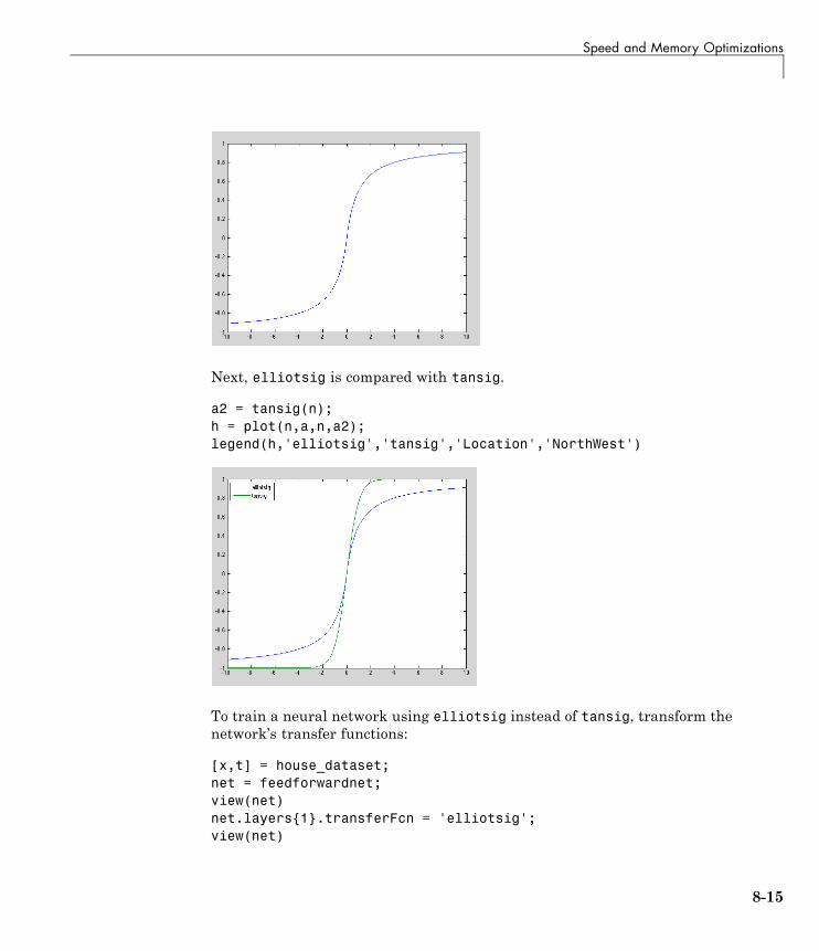
Speed and Memory Optimizations
Next, elliotsig is compared with tansig.
a2 = tansig(n);h = plot(n,a,n,a2);legend(h,'elliotsig','tansig','Location','NorthWest')
To train a neural network using elliotsig instead of tansig, transform thenetwork’s transfer functions:
[x,t] = house_dataset;net = feedforwardnet;view(net)net.layers{1}.transferFcn = 'elliotsig';view(net)
8-15
8 Advanced Topics
net = train(net,x,t);y = net(x)
Here, the times to execute elliotsig and tansig are compared. elliotsigis approximately four times faster on the test system.
n = rand(1000,1000);tic,for i=1:100,a=tansig(n); end, tansigTime = toc;tic,for i=1:100,a=elliotsig(n); end, elliotTime = toc;speedup = tansigTime / elliotTime
speedup =
4.1406
However, while simulation is faster with elliotsig, training is notguaranteed to be faster, due to the different shapes of the two transferfunctions. Here, 10 networks are each trained for tansig and elliotsig, buttraining times vary significantly even on the same problem with the samenetwork.
[x,t] = house_dataset;tansigNet = feedforwardnet;tansigNet.trainParam.showWindow = false;elliotNet = tansigNet;elliotNet.layers{1}.transferFcn = 'elliotsig';for i=1:10, tic, net = train(tansigNet,x,t); tansigTime = toc, endfor i=1:10, tic, net = train(elliotNet,x,t), elliotTime = toc, end
8-16
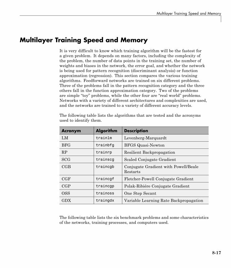
Multilayer Training Speed and Memory
Multilayer Training Speed and MemoryIt is very difficult to know which training algorithm will be the fastest fora given problem. It depends on many factors, including the complexity ofthe problem, the number of data points in the training set, the number ofweights and biases in the network, the error goal, and whether the networkis being used for pattern recognition (discriminant analysis) or functionapproximation (regression). This section compares the various trainingalgorithms. Feedforward networks are trained on six different problems.Three of the problems fall in the pattern recognition category and the threeothers fall in the function approximation category. Two of the problemsare simple “toy” problems, while the other four are “real world” problems.Networks with a variety of different architectures and complexities are used,and the networks are trained to a variety of different accuracy levels.
The following table lists the algorithms that are tested and the acronymsused to identify them.
Acronym Algorithm Description
LM trainlm Levenberg-Marquardt
BFG trainbfg BFGS Quasi-Newton
RP trainrp Resilient Backpropagation
SCG trainscg Scaled Conjugate Gradient
CGB traincgb Conjugate Gradient with Powell/BealeRestarts
CGF traincgf Fletcher-Powell Conjugate Gradient
CGP traincgp Polak-Ribiére Conjugate Gradient
OSS trainoss One Step Secant
GDX traingdx Variable Learning Rate Backpropagation
The following table lists the six benchmark problems and some characteristicsof the networks, training processes, and computers used.
8-17
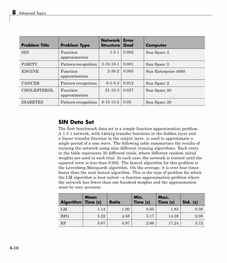
8 Advanced Topics
Problem Title Problem TypeNetworkStructure
ErrorGoal Computer
SIN Functionapproximation
1-5-1 0.002 Sun Sparc 2
PARITY Pattern recognition 3-10-10-1 0.001 Sun Sparc 2
ENGINE Functionapproximation
2-30-2 0.005 Sun Enterprise 4000
CANCER Pattern recognition 9-5-5-2 0.012 Sun Sparc 2
CHOLESTEROL Functionapproximation
21-15-3 0.027 Sun Sparc 20
DIABETES Pattern recognition 8-15-15-2 0.05 Sun Sparc 20
SIN Data SetThe first benchmark data set is a simple function approximation problem.A 1-5-1 network, with tansig transfer functions in the hidden layer anda linear transfer function in the output layer, is used to approximate asingle period of a sine wave. The following table summarizes the results oftraining the network using nine different training algorithms. Each entryin the table represents 30 different trials, where different random initialweights are used in each trial. In each case, the network is trained until thesquared error is less than 0.002. The fastest algorithm for this problem isthe Levenberg-Marquardt algorithm. On the average, it is over four timesfaster than the next fastest algorithm. This is the type of problem for whichthe LM algorithm is best suited—a function approximation problem wherethe network has fewer than one hundred weights and the approximationmust be very accurate.
AlgorithmMeanTime (s) Ratio
Min.Time (s)
Max.Time (s) Std. (s)
LM 1.14 1.00 0.65 1.83 0.38
BFG 5.22 4.58 3.17 14.38 2.08
RP 5.67 4.97 2.66 17.24 3.72
8-18
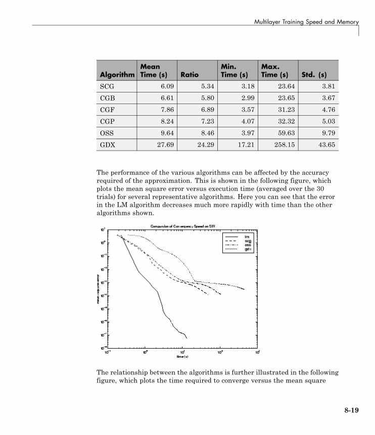
Multilayer Training Speed and Memory
AlgorithmMeanTime (s) Ratio
Min.Time (s)
Max.Time (s) Std. (s)
SCG 6.09 5.34 3.18 23.64 3.81
CGB 6.61 5.80 2.99 23.65 3.67
CGF 7.86 6.89 3.57 31.23 4.76
CGP 8.24 7.23 4.07 32.32 5.03
OSS 9.64 8.46 3.97 59.63 9.79
GDX 27.69 24.29 17.21 258.15 43.65
The performance of the various algorithms can be affected by the accuracyrequired of the approximation. This is shown in the following figure, whichplots the mean square error versus execution time (averaged over the 30trials) for several representative algorithms. Here you can see that the errorin the LM algorithm decreases much more rapidly with time than the otheralgorithms shown.
The relationship between the algorithms is further illustrated in the followingfigure, which plots the time required to converge versus the mean square
8-19
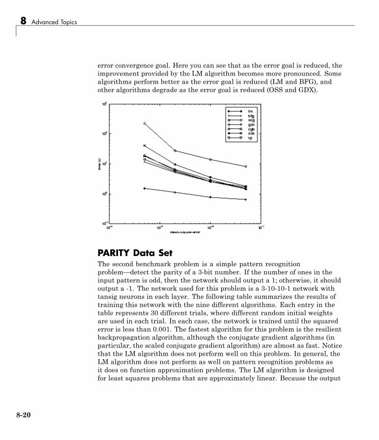
8 Advanced Topics
error convergence goal. Here you can see that as the error goal is reduced, theimprovement provided by the LM algorithm becomes more pronounced. Somealgorithms perform better as the error goal is reduced (LM and BFG), andother algorithms degrade as the error goal is reduced (OSS and GDX).
PARITY Data SetThe second benchmark problem is a simple pattern recognitionproblem—detect the parity of a 3-bit number. If the number of ones in theinput pattern is odd, then the network should output a 1; otherwise, it shouldoutput a -1. The network used for this problem is a 3-10-10-1 network withtansig neurons in each layer. The following table summarizes the results oftraining this network with the nine different algorithms. Each entry in thetable represents 30 different trials, where different random initial weightsare used in each trial. In each case, the network is trained until the squarederror is less than 0.001. The fastest algorithm for this problem is the resilientbackpropagation algorithm, although the conjugate gradient algorithms (inparticular, the scaled conjugate gradient algorithm) are almost as fast. Noticethat the LM algorithm does not perform well on this problem. In general, theLM algorithm does not perform as well on pattern recognition problems asit does on function approximation problems. The LM algorithm is designedfor least squares problems that are approximately linear. Because the output
8-20
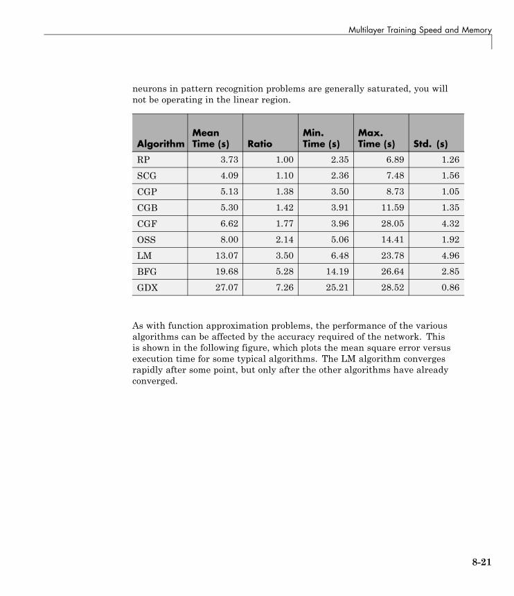
Multilayer Training Speed and Memory
neurons in pattern recognition problems are generally saturated, you willnot be operating in the linear region.
AlgorithmMeanTime (s) Ratio
Min.Time (s)
Max.Time (s) Std. (s)
RP 3.73 1.00 2.35 6.89 1.26
SCG 4.09 1.10 2.36 7.48 1.56
CGP 5.13 1.38 3.50 8.73 1.05
CGB 5.30 1.42 3.91 11.59 1.35
CGF 6.62 1.77 3.96 28.05 4.32
OSS 8.00 2.14 5.06 14.41 1.92
LM 13.07 3.50 6.48 23.78 4.96
BFG 19.68 5.28 14.19 26.64 2.85
GDX 27.07 7.26 25.21 28.52 0.86
As with function approximation problems, the performance of the variousalgorithms can be affected by the accuracy required of the network. Thisis shown in the following figure, which plots the mean square error versusexecution time for some typical algorithms. The LM algorithm convergesrapidly after some point, but only after the other algorithms have alreadyconverged.
8-21
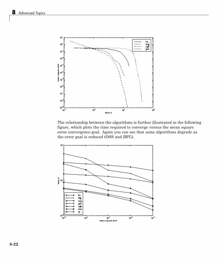
8 Advanced Topics
The relationship between the algorithms is further illustrated in the followingfigure, which plots the time required to converge versus the mean squareerror convergence goal. Again you can see that some algorithms degrade asthe error goal is reduced (OSS and BFG).
8-22
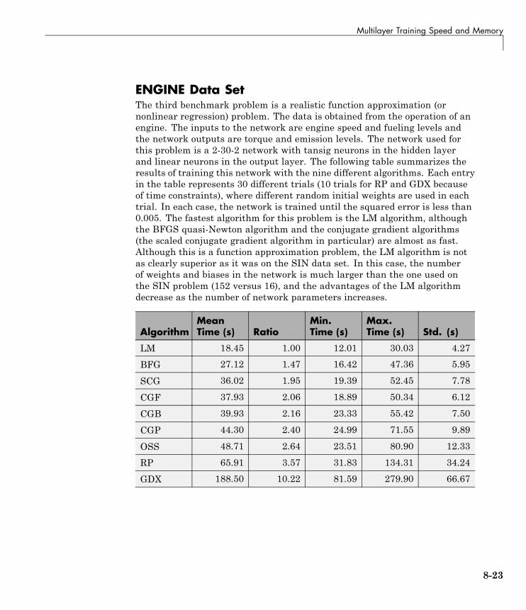
Multilayer Training Speed and Memory
ENGINE Data SetThe third benchmark problem is a realistic function approximation (ornonlinear regression) problem. The data is obtained from the operation of anengine. The inputs to the network are engine speed and fueling levels andthe network outputs are torque and emission levels. The network used forthis problem is a 2-30-2 network with tansig neurons in the hidden layerand linear neurons in the output layer. The following table summarizes theresults of training this network with the nine different algorithms. Each entryin the table represents 30 different trials (10 trials for RP and GDX becauseof time constraints), where different random initial weights are used in eachtrial. In each case, the network is trained until the squared error is less than0.005. The fastest algorithm for this problem is the LM algorithm, althoughthe BFGS quasi-Newton algorithm and the conjugate gradient algorithms(the scaled conjugate gradient algorithm in particular) are almost as fast.Although this is a function approximation problem, the LM algorithm is notas clearly superior as it was on the SIN data set. In this case, the numberof weights and biases in the network is much larger than the one used onthe SIN problem (152 versus 16), and the advantages of the LM algorithmdecrease as the number of network parameters increases.
AlgorithmMeanTime (s) Ratio
Min.Time (s)
Max.Time (s) Std. (s)
LM 18.45 1.00 12.01 30.03 4.27
BFG 27.12 1.47 16.42 47.36 5.95
SCG 36.02 1.95 19.39 52.45 7.78
CGF 37.93 2.06 18.89 50.34 6.12
CGB 39.93 2.16 23.33 55.42 7.50
CGP 44.30 2.40 24.99 71.55 9.89
OSS 48.71 2.64 23.51 80.90 12.33
RP 65.91 3.57 31.83 134.31 34.24
GDX 188.50 10.22 81.59 279.90 66.67
8-23
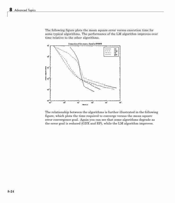
8 Advanced Topics
The following figure plots the mean square error versus execution time forsome typical algorithms. The performance of the LM algorithm improves overtime relative to the other algorithms.
The relationship between the algorithms is further illustrated in the followingfigure, which plots the time required to converge versus the mean squareerror convergence goal. Again you can see that some algorithms degrade asthe error goal is reduced (GDX and RP), while the LM algorithm improves.
8-24
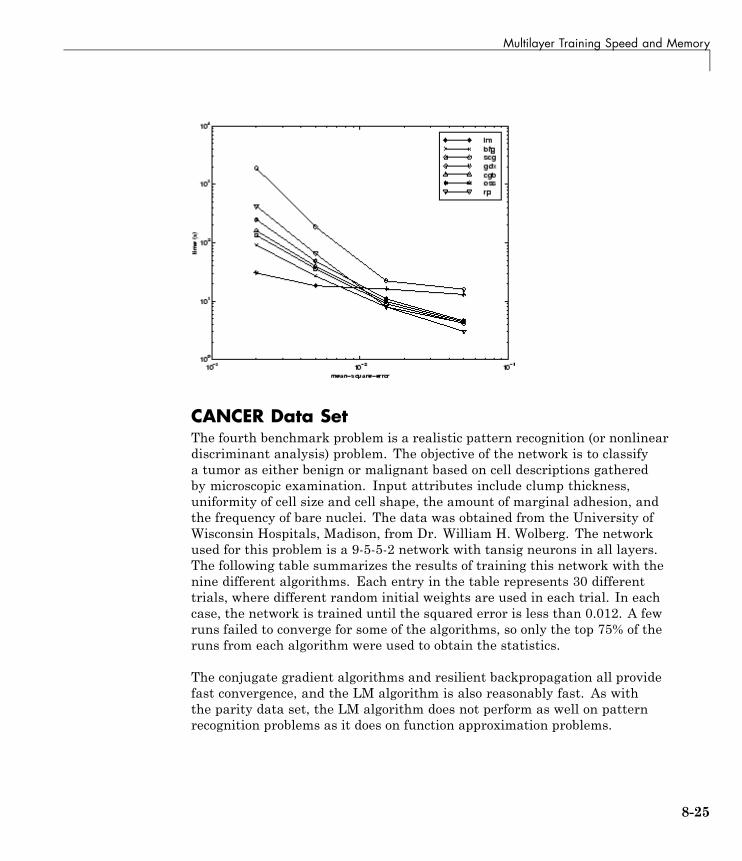
Multilayer Training Speed and Memory
CANCER Data SetThe fourth benchmark problem is a realistic pattern recognition (or nonlineardiscriminant analysis) problem. The objective of the network is to classifya tumor as either benign or malignant based on cell descriptions gatheredby microscopic examination. Input attributes include clump thickness,uniformity of cell size and cell shape, the amount of marginal adhesion, andthe frequency of bare nuclei. The data was obtained from the University ofWisconsin Hospitals, Madison, from Dr. William H. Wolberg. The networkused for this problem is a 9-5-5-2 network with tansig neurons in all layers.The following table summarizes the results of training this network with thenine different algorithms. Each entry in the table represents 30 differenttrials, where different random initial weights are used in each trial. In eachcase, the network is trained until the squared error is less than 0.012. A fewruns failed to converge for some of the algorithms, so only the top 75% of theruns from each algorithm were used to obtain the statistics.
The conjugate gradient algorithms and resilient backpropagation all providefast convergence, and the LM algorithm is also reasonably fast. As withthe parity data set, the LM algorithm does not perform as well on patternrecognition problems as it does on function approximation problems.
8-25
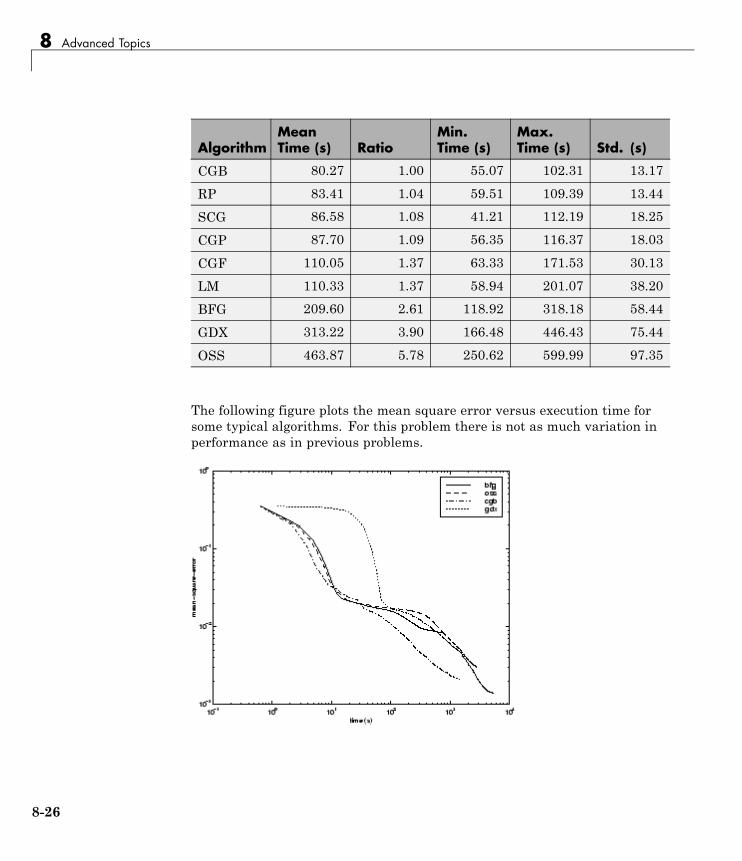
8 Advanced Topics
AlgorithmMeanTime (s) Ratio
Min.Time (s)
Max.Time (s) Std. (s)
CGB 80.27 1.00 55.07 102.31 13.17
RP 83.41 1.04 59.51 109.39 13.44
SCG 86.58 1.08 41.21 112.19 18.25
CGP 87.70 1.09 56.35 116.37 18.03
CGF 110.05 1.37 63.33 171.53 30.13
LM 110.33 1.37 58.94 201.07 38.20
BFG 209.60 2.61 118.92 318.18 58.44
GDX 313.22 3.90 166.48 446.43 75.44
OSS 463.87 5.78 250.62 599.99 97.35
The following figure plots the mean square error versus execution time forsome typical algorithms. For this problem there is not as much variation inperformance as in previous problems.
8-26
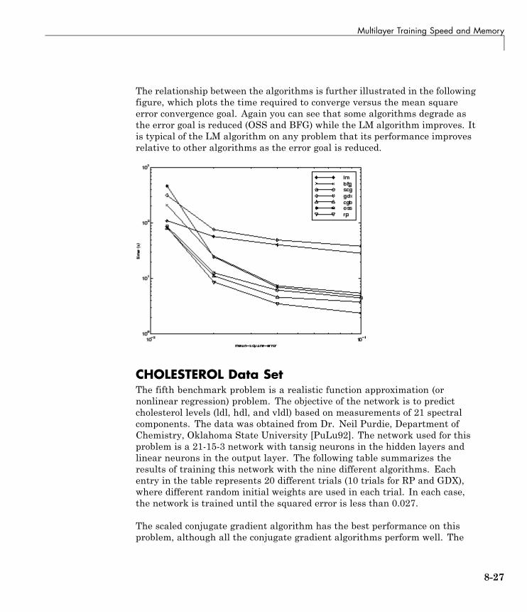
Multilayer Training Speed and Memory
The relationship between the algorithms is further illustrated in the followingfigure, which plots the time required to converge versus the mean squareerror convergence goal. Again you can see that some algorithms degrade asthe error goal is reduced (OSS and BFG) while the LM algorithm improves. Itis typical of the LM algorithm on any problem that its performance improvesrelative to other algorithms as the error goal is reduced.
CHOLESTEROL Data SetThe fifth benchmark problem is a realistic function approximation (ornonlinear regression) problem. The objective of the network is to predictcholesterol levels (ldl, hdl, and vldl) based on measurements of 21 spectralcomponents. The data was obtained from Dr. Neil Purdie, Department ofChemistry, Oklahoma State University [PuLu92]. The network used for thisproblem is a 21-15-3 network with tansig neurons in the hidden layers andlinear neurons in the output layer. The following table summarizes theresults of training this network with the nine different algorithms. Eachentry in the table represents 20 different trials (10 trials for RP and GDX),where different random initial weights are used in each trial. In each case,the network is trained until the squared error is less than 0.027.
The scaled conjugate gradient algorithm has the best performance on thisproblem, although all the conjugate gradient algorithms perform well. The
8-27
8 Advanced Topics
LM algorithm does not perform as well on this function approximationproblem as it did on the other two. That is because the number of weightsand biases in the network has increased again (378 versus 152 versus 16).As the number of parameters increases, the computation required in the LMalgorithm increases geometrically.
AlgorithmMeanTime (s) Ratio
Min.Time (s)
Max.Time (s) Std. (s)
SCG 99.73 1.00 83.10 113.40 9.93
CGP 121.54 1.22 101.76 162.49 16.34
CGB 124.06 1.2 107.64 146.90 14.62
CGF 136.04 1.36 106.46 167.28 17.67
LM 261.50 2.62 103.52 398.45 102.06
OSS 268.55 2.69 197.84 372.99 56.79
BFG 550.92 5.52 471.61 676.39 46.59
RP 1519.00 15.23 581.17 2256.10 557.34
GDX 3169.50 31.78 2514.90 4168.20 610.52
The following figure plots the mean square error versus execution timefor some typical algorithms. For this problem, you can see that the LMalgorithm is able to drive the mean square error to a lower level than theother algorithms. The SCG and RP algorithms provide the fastest initialconvergence.
8-28
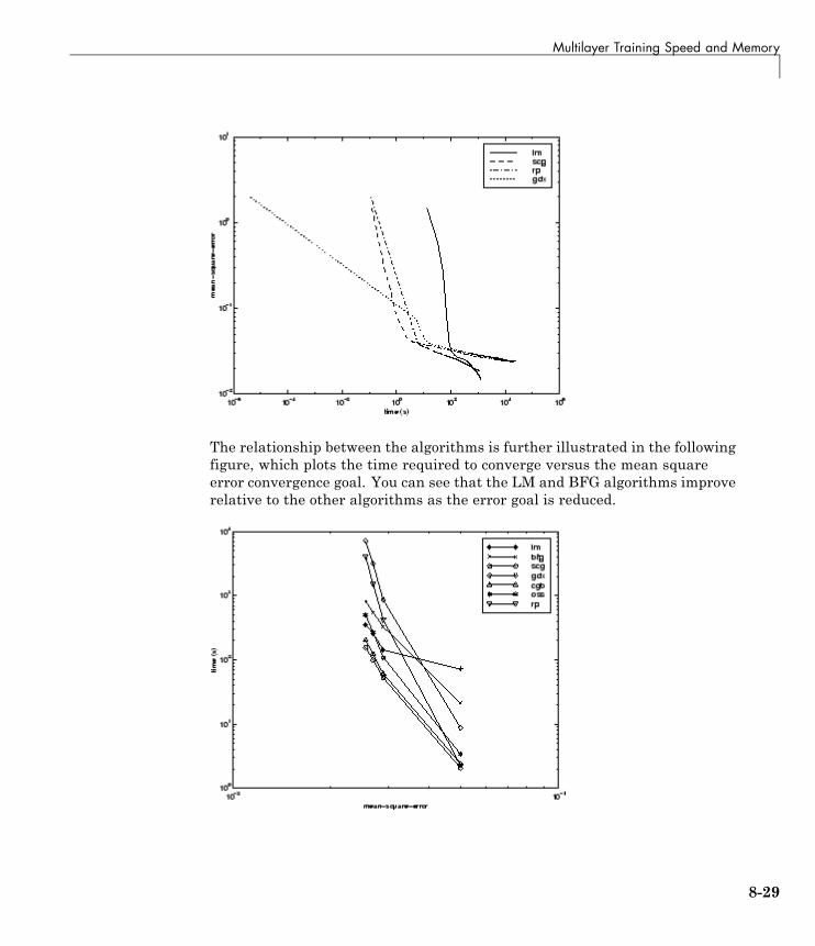
Multilayer Training Speed and Memory
The relationship between the algorithms is further illustrated in the followingfigure, which plots the time required to converge versus the mean squareerror convergence goal. You can see that the LM and BFG algorithms improverelative to the other algorithms as the error goal is reduced.
8-29
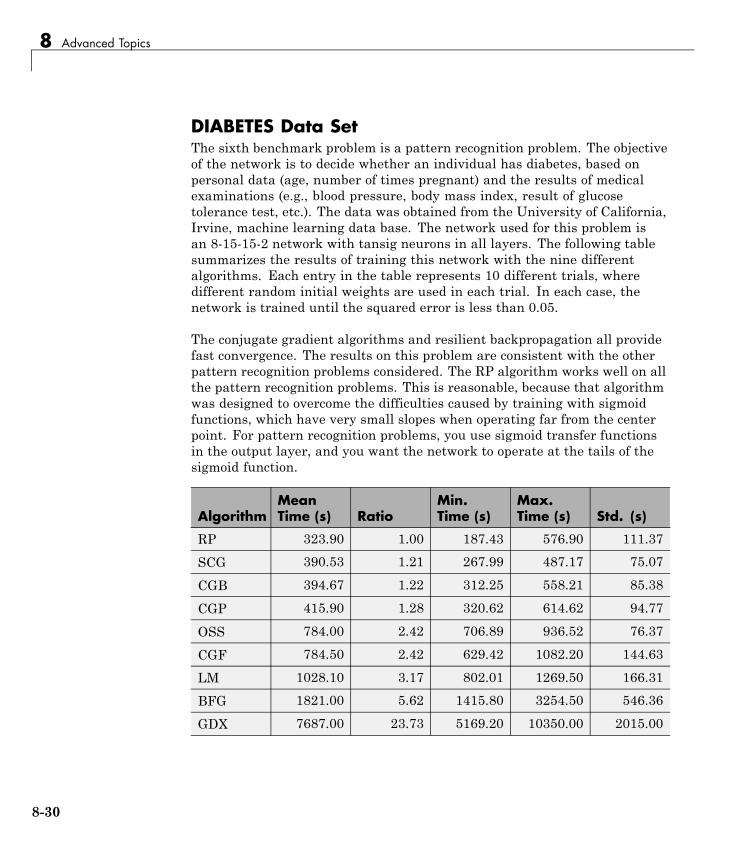
8 Advanced Topics
DIABETES Data SetThe sixth benchmark problem is a pattern recognition problem. The objectiveof the network is to decide whether an individual has diabetes, based onpersonal data (age, number of times pregnant) and the results of medicalexaminations (e.g., blood pressure, body mass index, result of glucosetolerance test, etc.). The data was obtained from the University of California,Irvine, machine learning data base. The network used for this problem isan 8-15-15-2 network with tansig neurons in all layers. The following tablesummarizes the results of training this network with the nine differentalgorithms. Each entry in the table represents 10 different trials, wheredifferent random initial weights are used in each trial. In each case, thenetwork is trained until the squared error is less than 0.05.
The conjugate gradient algorithms and resilient backpropagation all providefast convergence. The results on this problem are consistent with the otherpattern recognition problems considered. The RP algorithm works well on allthe pattern recognition problems. This is reasonable, because that algorithmwas designed to overcome the difficulties caused by training with sigmoidfunctions, which have very small slopes when operating far from the centerpoint. For pattern recognition problems, you use sigmoid transfer functionsin the output layer, and you want the network to operate at the tails of thesigmoid function.
AlgorithmMeanTime (s) Ratio
Min.Time (s)
Max.Time (s) Std. (s)
RP 323.90 1.00 187.43 576.90 111.37
SCG 390.53 1.21 267.99 487.17 75.07
CGB 394.67 1.22 312.25 558.21 85.38
CGP 415.90 1.28 320.62 614.62 94.77
OSS 784.00 2.42 706.89 936.52 76.37
CGF 784.50 2.42 629.42 1082.20 144.63
LM 1028.10 3.17 802.01 1269.50 166.31
BFG 1821.00 5.62 1415.80 3254.50 546.36
GDX 7687.00 23.73 5169.20 10350.00 2015.00
8-30
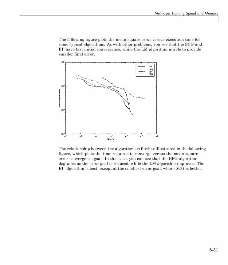
Multilayer Training Speed and Memory
The following figure plots the mean square error versus execution time forsome typical algorithms. As with other problems, you see that the SCG andRP have fast initial convergence, while the LM algorithm is able to providesmaller final error.
The relationship between the algorithms is further illustrated in the followingfigure, which plots the time required to converge versus the mean squareerror convergence goal. In this case, you can see that the BFG algorithmdegrades as the error goal is reduced, while the LM algorithm improves. TheRP algorithm is best, except at the smallest error goal, where SCG is better.
8-31
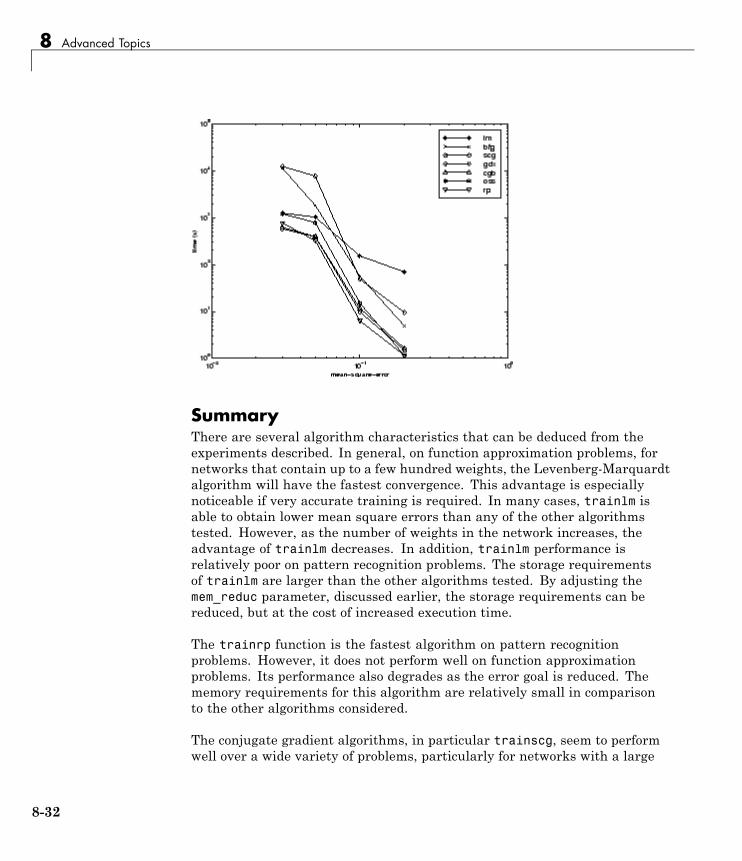
8 Advanced Topics
SummaryThere are several algorithm characteristics that can be deduced from theexperiments described. In general, on function approximation problems, fornetworks that contain up to a few hundred weights, the Levenberg-Marquardtalgorithm will have the fastest convergence. This advantage is especiallynoticeable if very accurate training is required. In many cases, trainlm isable to obtain lower mean square errors than any of the other algorithmstested. However, as the number of weights in the network increases, theadvantage of trainlm decreases. In addition, trainlm performance isrelatively poor on pattern recognition problems. The storage requirementsof trainlm are larger than the other algorithms tested. By adjusting themem_reduc parameter, discussed earlier, the storage requirements can bereduced, but at the cost of increased execution time.
The trainrp function is the fastest algorithm on pattern recognitionproblems. However, it does not perform well on function approximationproblems. Its performance also degrades as the error goal is reduced. Thememory requirements for this algorithm are relatively small in comparisonto the other algorithms considered.
The conjugate gradient algorithms, in particular trainscg, seem to performwell over a wide variety of problems, particularly for networks with a large
8-32
Multilayer Training Speed and Memory
number of weights. The SCG algorithm is almost as fast as the LM algorithmon function approximation problems (faster for large networks) and is almostas fast as trainrp on pattern recognition problems. Its performance doesnot degrade as quickly as trainrp performance does when the error isreduced. The conjugate gradient algorithms have relatively modest memoryrequirements.
The performance of trainbfg is similar to that of trainlm. It does not requireas much storage as trainlm, but the computation required does increasegeometrically with the size of the network, because the equivalent of a matrixinverse must be computed at each iteration.
The variable learning rate algorithm traingdx is usually much slower thanthe other methods, and has about the same storage requirements as trainrp,but it can still be useful for some problems. There are certain situations inwhich it is better to converge more slowly. For example, when using earlystopping you can have inconsistent results if you use an algorithm thatconverges too quickly. You might overshoot the point at which the error onthe validation set is minimized.
8-33
8 Advanced Topics
Improving GeneralizationOne of the problems that occur during neural network training is calledoverfitting. The error on the training set is driven to a very small value, butwhen new data is presented to the network the error is large. The networkhas memorized the training examples, but it has not learned to generalize tonew situations.
The following figure shows the response of a 1-20-1 neural network thathas been trained to approximate a noisy sine function. The underlying sinefunction is shown by the dotted line, the noisy measurements are given by the+ symbols, and the neural network response is given by the solid line. Clearlythis network has overfitted the data and will not generalize well.
One method for improving network generalization is to use a network that isjust large enough to provide an adequate fit. The larger network you use, themore complex the functions the network can create. If you use a small enoughnetwork, it will not have enough power to overfit the data. Run the NeuralNetwork Design example nnd11gn [HDB96] to investigate how reducing thesize of a network can prevent overfitting.
8-34
Improving Generalization
Unfortunately, it is difficult to know beforehand how large a network shouldbe for a specific application. There are two other methods for improvinggeneralization that are implemented in Neural Network Toolbox software:regularization and early stopping. The next sections describe these twotechniques and the routines to implement them.
Note that if the number of parameters in the network is much smaller thanthe total number of points in the training set, then there is little or no chanceof overfitting. If you can easily collect more data and increase the size of thetraining set, then there is no need to worry about the following techniques toprevent overfitting. The rest of this section only applies to those situations inwhich you want to make the most of a limited supply of data.
Early StoppingThe default method for improving generalization is called early stopping.This technique is automatically provided for all of the supervised networkcreation functions, including the backpropagation network creation functionssuch as newff.
In this technique the available data is divided into three subsets. Thefirst subset is the training set, which is used for computing the gradientand updating the network weights and biases. The second subset is thevalidation set. The error on the validation set is monitored during thetraining process. The validation error normally decreases during the initialphase of training, as does the training set error. However, when the networkbegins to overfit the data, the error on the validation set typically begins torise. When the validation error increases for a specified number of iterations(net.trainParam.max_fail), the training is stopped, and the weights andbiases at the minimum of the validation error are returned.
The test set error is not used during training, but it is used to comparedifferent models. It is also useful to plot the test set error during the trainingprocess. If the error in the test set reaches a minimum at a significantlydifferent iteration number than the validation set error, this might indicate apoor division of the data set.
There are four functions provided for dividing data into training, validationand test sets. They are dividerand (the default), divideblock, divideint,
8-35
8 Advanced Topics
and divideind. You can access or change the division function for yournetwork with this property:
net.divideFcn
Each of these functions takes parameters that customize its behavior. Thesevalues are stored and can be changed with the following network property:
net.divideParam
Index Data Division (divideind)Create a simple test problem. For the full data set, generate a noisy sine wavewith 201 input points ranging from −1 to 1 at steps of 0.01:
p = [-1:0.01:1];t = sin(2*pi*p)+0.1*randn(size(p));
Divide the data by index so that successive samples are assigned to thetraining set, validation set, and test set successively:
trainInd = 1:3:201valInd = 2:3:201;testInd = 3:3:201;[trainP,valP,testP] = divideind(p,trainInd,valInd,testInd);[trainT,valT,testT] = divideind(t,trainInd,valInd,testInd);
Random Data Division (dividerand)You can divide the input data randomly so that 60% of the samples areassigned to the training set, 20% to the validation set, and 20% to the testset, as follows:
[trainP,valP,testP,trainInd,valInd,testInd] = dividerand(p);
This function not only divides the input data, but also returns indices so thatyou can divide the target data accordingly using divideind:
[trainT,valT,testT] = divideind(t,trainInd,valInd,testInd);
8-36
Improving Generalization
Block Data Division (divideblock)You can also divide the input data randomly such that the first 60% of thesamples are assigned to the training set, the next 20% to the validation set,and the last 20% to the test set, as follows:
[trainP,valP,testP,trainInd,valInd,testInd] = divideblock(p);
Divide the target data accordingly using divideind:
[trainT,valT,testT] = divideind(t,trainInd,valInd,testInd);
Interleaved Data Division (divideint)Another way to divide the input data is to cycle samples between the trainingset, validation set, and test set according to percentages. You can interleave60% of the samples to the training set, 20% to the validation set and 20% tothe test set as follows:
[trainP,valP,testP,trainInd,valInd,testInd] = divideint(p);
Divide the target data accordingly using divideind.
[trainT,valT,testT] = divideind(t,trainInd,valInd,testInd);
RegularizationAnother method for improving generalization is called regularization. Thisinvolves modifying the performance function, which is normally chosen to bethe sum of squares of the network errors on the training set. The next sectionexplains how the performance function can be modified, and the followingsection describes a routine that automatically sets the optimal performancefunction to achieve the best generalization.
Modified Performance FunctionThe typical performance function used for training feedforward neuralnetworks is the mean sum of squares of the network errors.
F mseN
eN
tii
N
i ii
N= = = −
= =∑ ∑1 12
1
2
1
( ) ( )
8-37
8 Advanced Topics
It is possible to improve generalization if you modify the performance functionby adding a term that consists of the mean of the sum of squares of thenetwork weights and biases msereg = γmse + (1 − γ)msw,
where γ is the performance ratio, and
mswn
wjj
n=
=∑1 2
1
Using this performance function causes the network to have smaller weightsand biases, and this forces the network response to be smoother and lesslikely to overfit.
The following code reinitializes the previous network and retrains it usingthe BFGS algorithm with the regularized performance function. Here theperformance ratio is set to 0.5, which gives equal weight to the mean squareerrors and the mean square weights. (Data division is cancelled by settingnet.divideFcn so that the effects of msereg are isolated from early stopping.)
p = [-1 -1 2 2;0 5 0 5];t = [-1 -1 1 1];net=newff(p,t,3,{},'trainbfg');net.divideFcn = '';net.performFcn = 'msereg';net.performParam.ratio = 0.5;net.trainParam.show = 5;net.trainParam.epochs = 300;net.trainParam.goal = 1e-5;[net,tr]=train(net,p,t);
The problem with regularization is that it is difficult to determine theoptimum value for the performance ratio parameter. If you make thisparameter too large, you might get overfitting. If the ratio is too small, thenetwork does not adequately fit the training data. The next section describesa routine that automatically sets the regularization parameters.
8-38
Improving Generalization
Automated Regularization (trainbr)It is desirable to determine the optimal regularization parameters in anautomated fashion. One approach to this process is the Bayesian frameworkof David MacKay [MacK92]. In this framework, the weights and biases of thenetwork are assumed to be random variables with specified distributions. Theregularization parameters are related to the unknown variances associatedwith these distributions. You can then estimate these parameters usingstatistical techniques.
A detailed discussion of Bayesian regularization is beyond the scope of thisuser guide. A detailed discussion of the use of Bayesian regularization, incombination with Levenberg-Marquardt training, can be found in [FoHa97].
Bayesian regularization has been implemented in the function trainbr.The following code shows how you can train a 1-20-1 network usingthis function to approximate the noisy sine wave shown in the figure in“Improving Generalization” on page 8-34. (Data division is cancelled bysetting net.divideFcn so that the effects of trainbr are isolated from earlystopping.)
p = [-1:.05:1];t = sin(2*pi*p)+0.1*randn(size(p));net=newff(p,t,20,{},'trainbr');net.divideFcn ='';net.trainParam.show = 10;net.trainParam.epochs = 50;randn('seed',192736547);net = init(net);[net,tr]=train(net,p,t);
One feature of this algorithm is that it provides a measure of how manynetwork parameters (weights and biases) are being effectively used by thenetwork. In this case, the final trained network uses approximately 12parameters (indicated by #Par in the printout) out of the 61 total weightsand biases in the 1-20-1 network. This effective number of parametersshould remain approximately the same, no matter how large the number ofparameters in the network becomes. (This assumes that the network has beentrained for a sufficient number of iterations to ensure convergence.)
8-39
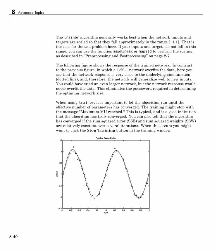
8 Advanced Topics
The trainbr algorithm generally works best when the network inputs andtargets are scaled so that they fall approximately in the range [−1,1]. That isthe case for the test problem here. If your inputs and targets do not fall in thisrange, you can use the function mapminmax or mapstd to perform the scaling,as described in “Preprocessing and Postprocessing” on page 2-7.
The following figure shows the response of the trained network. In contrastto the previous figure, in which a 1-20-1 network overfits the data, here yousee that the network response is very close to the underlying sine function(dotted line), and, therefore, the network will generalize well to new inputs.You could have tried an even larger network, but the network response wouldnever overfit the data. This eliminates the guesswork required in determiningthe optimum network size.
When using trainbr, it is important to let the algorithm run until theeffective number of parameters has converged. The training might stop withthe message "Maximum MU reached." This is typical, and is a good indicationthat the algorithm has truly converged. You can also tell that the algorithmhas converged if the sum squared error (SSE) and sum squared weights (SSW)are relatively constant over several iterations. When this occurs you mightwant to click the Stop Training button in the training window.
8-40

Improving Generalization
Summary and Discussion of Early Stopping andRegularizationEarly stopping and regularization can ensure network generalization whenyou apply them properly.
For early stopping, you must be careful not to use an algorithm that convergestoo rapidly. If you are using a fast algorithm (like trainlm), set the trainingparameters so that the convergence is relatively slow. For example, set muto a relatively large value, such as 1, and set mu_dec and mu_inc to valuesclose to 1, such as 0.8 and 1.5, respectively. The training functions trainscgand trainbr usually work well with early stopping.
With early stopping, the choice of the validation set is also important. Thevalidation set should be representative of all points in the training set.
When you use Bayesian regularization, it is important to train the networkuntil it reaches convergence. The sum-squared error, the sum-squaredweights, and the effective number of parameters should reach constant valueswhen the network has converged.
With both early stopping and regularization, it is a good idea to train thenetwork starting from several different initial conditions. It is possible foreither method to fail in certain circumstances. By testing several differentinitial conditions, you can verify robust network performance.
When the data set is small and you are training function approximationnetworks, Bayesian regularization provides better generalization performancethan early stopping. This is because Bayesian regularization does not requirethat a validation data set be separate from the training data set; it uses allthe data.
To provide some insight into the performance of the algorithms, both earlystopping and Bayesian regularization were tested on several benchmark datasets, which are listed in the following table.
8-41
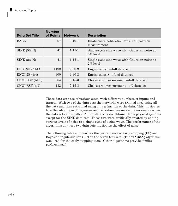
8 Advanced Topics
Data Set TitleNumberof Points Network Description
BALL 67 2-10-1 Dual-sensor calibration for a ball positionmeasurement
SINE (5% N) 41 1-15-1 Single-cycle sine wave with Gaussian noise at5% level
SINE (2% N) 41 1-15-1 Single-cycle sine wave with Gaussian noise at2% level
ENGINE (ALL) 1199 2-30-2 Engine sensor—full data set
ENGINE (1/4) 300 2-30-2 Engine sensor—1/4 of data set
CHOLEST (ALL) 264 5-15-3 Cholesterol measurement—full data set
CHOLEST (1/2) 132 5-15-3 Cholesterol measurement—1/2 data set
These data sets are of various sizes, with different numbers of inputs andtargets. With two of the data sets the networks were trained once using allthe data and then retrained using only a fraction of the data. This illustrateshow the advantage of Bayesian regularization becomes more noticeable whenthe data sets are smaller. All the data sets are obtained from physical systemsexcept for the SINE data sets. These two were artificially created by addingvarious levels of noise to a single cycle of a sine wave. The performance of thealgorithms on these two data sets illustrates the effect of noise.
The following table summarizes the performance of early stopping (ES) andBayesian regularization (BR) on the seven test sets. (The trainscg algorithmwas used for the early stopping tests. Other algorithms provide similarperformance.)
8-42
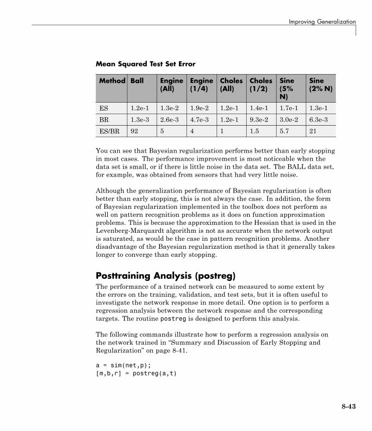
Improving Generalization
Mean Squared Test Set Error
Method Ball Engine(All)
Engine(1/4)
Choles(All)
Choles(1/2)
Sine(5%N)
Sine(2% N)
ES 1.2e-1 1.3e-2 1.9e-2 1.2e-1 1.4e-1 1.7e-1 1.3e-1
BR 1.3e-3 2.6e-3 4.7e-3 1.2e-1 9.3e-2 3.0e-2 6.3e-3
ES/BR 92 5 4 1 1.5 5.7 21
You can see that Bayesian regularization performs better than early stoppingin most cases. The performance improvement is most noticeable when thedata set is small, or if there is little noise in the data set. The BALL data set,for example, was obtained from sensors that had very little noise.
Although the generalization performance of Bayesian regularization is oftenbetter than early stopping, this is not always the case. In addition, the formof Bayesian regularization implemented in the toolbox does not perform aswell on pattern recognition problems as it does on function approximationproblems. This is because the approximation to the Hessian that is used in theLevenberg-Marquardt algorithm is not as accurate when the network outputis saturated, as would be the case in pattern recognition problems. Anotherdisadvantage of the Bayesian regularization method is that it generally takeslonger to converge than early stopping.
Posttraining Analysis (postreg)The performance of a trained network can be measured to some extent bythe errors on the training, validation, and test sets, but it is often useful toinvestigate the network response in more detail. One option is to perform aregression analysis between the network response and the correspondingtargets. The routine postreg is designed to perform this analysis.
The following commands illustrate how to perform a regression analysis onthe network trained in “Summary and Discussion of Early Stopping andRegularization” on page 8-41.
a = sim(net,p);[m,b,r] = postreg(a,t)
8-43
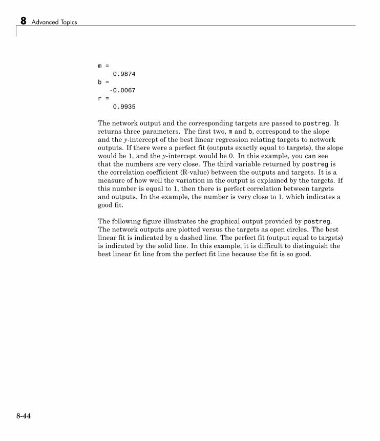
8 Advanced Topics
m =0.9874
b =-0.0067
r =0.9935
The network output and the corresponding targets are passed to postreg. Itreturns three parameters. The first two, m and b, correspond to the slopeand the y-intercept of the best linear regression relating targets to networkoutputs. If there were a perfect fit (outputs exactly equal to targets), the slopewould be 1, and the y-intercept would be 0. In this example, you can seethat the numbers are very close. The third variable returned by postreg isthe correlation coefficient (R-value) between the outputs and targets. It is ameasure of how well the variation in the output is explained by the targets. Ifthis number is equal to 1, then there is perfect correlation between targetsand outputs. In the example, the number is very close to 1, which indicates agood fit.
The following figure illustrates the graphical output provided by postreg.The network outputs are plotted versus the targets as open circles. The bestlinear fit is indicated by a dashed line. The perfect fit (output equal to targets)is indicated by the solid line. In this example, it is difficult to distinguish thebest linear fit line from the perfect fit line because the fit is so good.
8-44
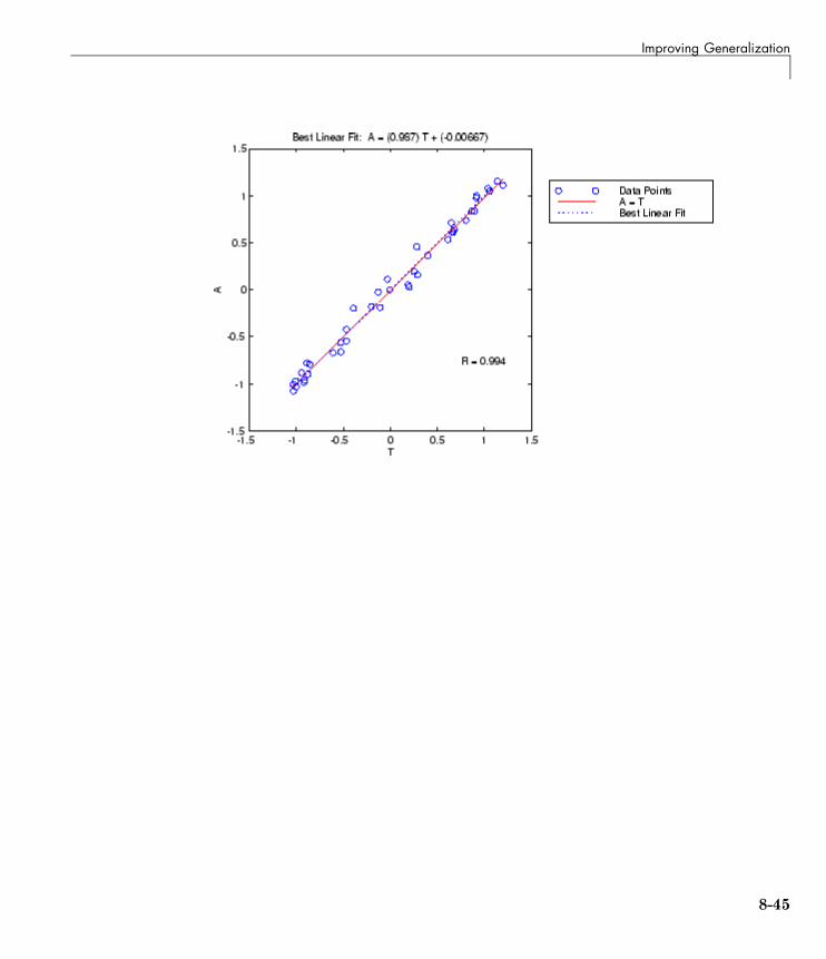
Improving Generalization
8-45
8 Advanced Topics
Custom NetworksNeural Network Toolbox software provides a flexible network object type thatallows many kinds of networks to be created and then used with functionssuch as init, sim, and train.
Type the following to see all the network creation functions in the toolbox.
help nnnetwork
This flexibility is possible because networks have an object-orientedrepresentation. The representation allows you to define various architecturesand assign various algorithms to those architectures.
To create custom networks, start with an empty network (obtained with thenetwork function) and set its properties as desired.
net = network
The network object consists of many properties that you can set to specify thestructure and behavior of your network.
The following sections show how to create a custom network by using theseproperties.
Custom NetworkBefore you can build a network you need to know what it looks like. Fordramatic purposes (and to give the toolbox a workout) this section leads youthrough the creation of the wild and complicated network shown below.
8-46
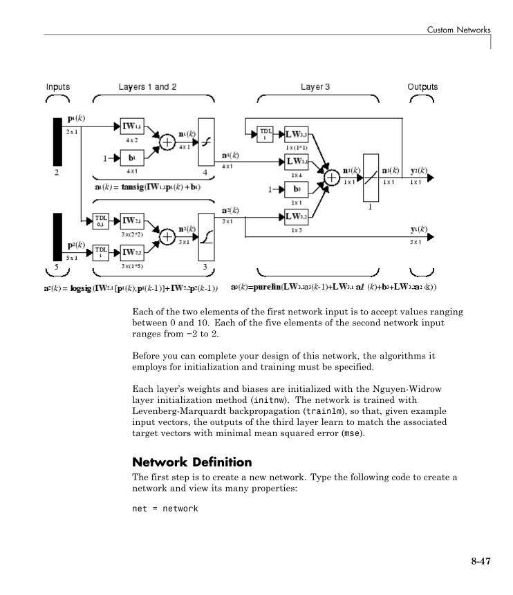
Custom Networks
Each of the two elements of the first network input is to accept values rangingbetween 0 and 10. Each of the five elements of the second network inputranges from −2 to 2.
Before you can complete your design of this network, the algorithms itemploys for initialization and training must be specified.
Each layer’s weights and biases are initialized with the Nguyen-Widrowlayer initialization method (initnw). The network is trained withLevenberg-Marquardt backpropagation (trainlm), so that, given exampleinput vectors, the outputs of the third layer learn to match the associatedtarget vectors with minimal mean squared error (mse).
Network DefinitionThe first step is to create a new network. Type the following code to create anetwork and view its many properties:
net = network
8-47
8 Advanced Topics
Architecture PropertiesThe first group of properties displayed is labeled architecture properties.These properties allow you to select the number of inputs and layers andtheir connections.
Number of Inputs and Layers. The first two properties displayed arenumInputs and numLayers. These properties allow you to select how manyinputs and layers you want the network to have.
net =Neural Network object:architecture:
numInputs: 0numLayers: 0...
Note that the network has no inputs or layers at this time.
Change that by setting these properties to the number of inputs and numberof layers in the custom network diagram.
net.numInputs = 2;net.numLayers = 3;
net.numInputs is the number of input sources, not the number of elements inan input vector (net.inputs{i}.size).
Bias Connections. Type net and press Enter to view its properties again.The network now has two inputs and three layers.
net =Neural Network object:architecture:
numInputs: 2numLayers: 3
Examine the next four properties:
biasConnect: [0; 0; 0]inputConnect: [0 0; 0 0; 0 0]layerConnect: [0 0 0; 0 0 0; 0 0 0]
8-48
Custom Networks
outputConnect: [0 0 0]
These matrices of 1s and 0s represent the presence and absence of bias, inputweight, layer weight, and output connections. They are currently all zeros,indicating that the network does not have any such connections.
The bias connection matrix is a 3-by-1 vector. To create a bias connection tothe ith layer you can set net.biasConnect(i) to 1. Specify that the firstand third layers are to have bias connections, as the diagram indicates, bytyping the following code:
net.biasConnect(1) = 1;net.biasConnect(3) = 1;
You could also define those connections with a single line of code.
net.biasConnect = [1; 0; 1];
Input and Layer Weight Connections. The input connectionmatrix is 3-by-2, representing the presence of connections from twosources (the two inputs) to three destinations (the three layers). Thus,net.inputConnect(i,j) represents the presence of an input weightconnection going to the ith layer from the jth input.
To connect the first input to the first and second layers, and the second inputto the second layer (as indicated by the custom network diagram), type
net.inputConnect(1,1) = 1;net.inputConnect(2,1) = 1;net.inputConnect(2,2) = 1;
or this single line of code:
net.inputConnect = [1 0; 1 1; 0 0];
Similarly, net.layerConnect(i.j) represents the presence of a layer-weightconnection going to the ith layer from the jth layer. Connect layers 1, 2, and 3to layer 3 as follows:
net.layerConnect = [0 0 0; 0 0 0; 1 1 1];
8-49
8 Advanced Topics
Output Connections. The output connections are a 1-by-3 matrix, indicatingthat they connect to one destination (the external world) from three sources(the three layers).
To connect layers 2 and 3 to the network output, type
net.outputConnect = [0 1 1];
Number of OutputsType net and press Enter to view the updated properties. The final threearchitecture properties are read-only values, which means their values aredetermined by the choices made for other properties. The first read-onlyproperty is the number of outputs:
numOutputs: 2 (read-only)
By defining output connection from layers 2 and 3, you specified that thenetwork has two outputs.
Subobject PropertiesThe next group of properties is
subobject structures:inputs: {2x1 cell} of inputslayers: {3x1 cell} of layers
outputs: {1x3 cell} containing 1 outputbiases: {3x1 cell} containing 2 biases
inputWeights: {3x2 cell} containing 3 input weightslayerWeights: {3x3 cell} containing 3 layer weights
InputsWhen you set the number of inputs (net.numInputs) to 2, the inputs propertybecomes a cell array of two input structures. Each ith input structure(net.inputs{i}) contains additional properties associated with the ith input.
To see how the input structures are arranged, type
8-50
Custom Networks
net.inputsans =
[1x1 struct][1x1 struct]
To see the properties associated with the first input, type
net.inputs{1}
The properties appear as follows:
ans =exampleInput: [0 1]processFcns: {}
processParams: {}processSettings: {}processedRange: [0 1]processedSize: 1
range: [0 1]size: 1
userdata: [1x1 struct]
If you set the exampleInput property, the range, size, processedSize,and processedRange properties will automatically be updated to match theproperties of the value of exampleInput.
Set the exampleInput property as follows:
net.inputs{1}.exampleInput = [0 10 5; 0 3 10];
If you examine the structure of the first input again, you see that it now hasnew values.
The property processFcns can be set to one or more processing functions.Type help nnprocess to see a list of these functions.
Set the second input vector ranges to be from −2 to 2 for five elements asfollows:
net.inputs{1}.processFcns = {'removeconstantrows','mapminmax'};
8-51
8 Advanced Topics
View the new input properties. You will see that processParams,processSettings, processedRange and processedSize have all beenupdated to reflect that inputs will be processed using removeconstantrowsand mapminmax before being given to the network when the network issimulated or trained. The property processParams contains the defaultparameters for each processing function. You can alter these values, if youlike. See the reference page for each processing function to learn more abouttheir parameters.
You can set the size of an input directly when no processing functions are used:
net.inputs{2}.size = 5;
Layers. When you set the number of layers (net.numLayers) to 3, the layersproperty becomes a cell array of three-layer structures. Type the followingline of code to see the properties associated with the first layer.
net.layers{1}ans =
dimensions: 1distanceFcn: 'dist'
distances: 0initFcn: 'initwb'
netInputFcn: 'netsum'netInputParam: [1x1 struct]
positions: 0size: 1
topologyFcn: 'hextop'transferFcn: 'purelin'
transferParam: [1x1 struct]userdata: [1x1 struct]
Type the following three lines of code to change the first layer’s size to 4neurons, its transfer function to tansig, and its initialization function to theNguyen-Widrow function, as required for the custom network diagram.
net.layers{1}.size = 4;net.layers{1}.transferFcn = 'tansig';net.layers{1}.initFcn = 'initnw';
8-52
Custom Networks
The second layer is to have three neurons, the logsig transfer function, andbe initialized with initnw. Set the second layer’s properties to the desiredvalues as follows:
net.layers{2}.size = 3;net.layers{2}.transferFcn = 'logsig';net.layers{2}.initFcn = 'initnw';
The third layer’s size and transfer function properties don’t need to bechanged, because the defaults match those shown in the network diagram.You only need to set its initialization function, as follows:
net.layers{3}.initFcn = 'initnw';
Outputs. Look at how the outputs property is arranged with this line of code.
net.outputsans =
[] [1x1 struct] [1x1 struct]
Note that outputs contains two output structures, one for layer 2 and one forlayer 3. This arrangement occurs automatically when net.outputConnectis set to [0 1 1].
View the second layer’s output structure with the following expression:
net.outputs{2}ans =
exampleOutput: []processFcns: {}
processParams: {}processSettings: {}processedRange: []processedSize: 1
range: []size: 3
userdata: [1x1 struct]
The size is automatically set to 3 when the second layer’s size(net.layers{2}.size) is set to that value. Look at the third layer’s outputstructure if you want to verify that it also has the correct size.
8-53
8 Advanced Topics
Outputs have processing properties that are automatically applied to targetvalues before they are used by the network during training. The sameprocessing settings are applied in reverse on layer output values before theyare returned as network output values during network simulation or training.
Similar to input-processing properties, setting the exampleOutput propertyautomatically causes size, range, processedSize and processedRange tobe updated. Setting processFcns to a cell array list of processing functionnames causes processParams, processSettings, processedRange to beupdated.You can then alter the processParam values, if you like.
Biases, Input Weights, and Layer Weights. Enter the followingcommands to see how bias and weight structures are arranged:
net.biasesnet.inputWeightsnet.layerWeights
Here are the results of typing net.biases:
ans =[1x1 struct]
[][1x1 struct]
Each contains a structure where the corresponding connections(net.biasConnect, net.inputConnect, and net.layerConnect) contain a 1.
Look at their structures with these lines of code:
net.biases{1}net.biases{3}net.inputWeights{1,1}net.inputWeights{2,1}net.inputWeights{2,2}net.layerWeights{3,1}net.layerWeights{3,2}net.layerWeights{3,3}
For example, typing net.biases{1} results in the following output:
8-54
Custom Networks
ans =initFcn: ''
learn: 1learnFcn: ''
learnParam: ''size: 4
userdata: [1x1 struct]
Specify the weights’ tap delay lines in accordance with the network diagramby setting each weight’s delays property:
net.inputWeights{2,1}.delays = [0 1];net.inputWeights{2,2}.delays = 1;net.layerWeights{3,3}.delays = 1;
Network FunctionsType net and press Return again to see the next set of properties.
functions:adaptFcn: (none)
divideFcn: (none)gradientFcn: (none)
initFcn: (none)performFcn: (none)plotFcns: {}trainFcn: (none)
Each of these properties defines a function for a basic network operation.
Set the initialization function to initlay so the network initializes itselfaccording to the layer initialization functions already set to initnw, theNguyen-Widrow initialization function.
net.initFcn = 'initlay';
This meets the initialization requirement of the network.
8-55
8 Advanced Topics
Set the performance function to mse (mean squared error) and the trainingfunction to trainlm (Levenberg-Marquardt backpropagation) to meet thefinal requirement of the custom network.
net.performFcn = 'mse';net.trainFcn = 'trainlm';
Set the divide function to dividerand (divide training data randomly).
net.divideFcn = 'dividerand';
During supervised training, the input and target data are randomly dividedinto training, test, and validation data sets. The network is trained on thetraining data until its performance begins to decrease on the validationdata, which signals that generalization has peaked. The test data provides acompletely independent test of network generalization.
Set the plot functions to plotperform (plot training, validation and testperformance) and plottrainstate (plot the state of the training algorithmwith respect to epochs).
net.plotFcns = {'plotperform','plottrainstate'};
Weight and Bias ValuesBefore initializing and training the network, look at the final group of networkproperties (aside from the userdata property).
weight and bias values:IW: {3x2 cell} containing 3 input weight matricesLW: {3x3 cell} containing 3 layer weight matricesb: {3x1 cell} containing 2 bias vectors
These cell arrays contain weight matrices and bias vectors in thesame positions that the connection properties (net.inputConnect,net.layerConnect, net.biasConnect) contain 1s and the subobjectproperties (net.inputWeights, net.layerWeights, net.biases) containstructures.
8-56
Custom Networks
Evaluating each of the following lines of code reveals that all the bias vectorsand weight matrices are set to zeros.
net.IW{1,1}, net.IW{2,1}, net.IW{2,2}net.LW{3,1}, net.LW{3,2}, net.LW{3,3}net.b{1}, net.b{3}
Each input weight net.IW{i,j}, layer weight net.LW{i,j}, and bias vectornet.b{i} has as many rows as the size of the ith layer (net.layers{i}.size).
Each input weight net.IW{i,j} has as many columns as the size of the jthinput (net.inputs{j}.size) multiplied by the number of its delay values(length(net.inputWeights{i,j}.delays)).
Likewise, each layer weight has as many columns as the size of the jthlayer (net.layers{j}.size) multiplied by the number of its delay values(length(net.layerWeights{i,j}.delays)).
Network Behavior
InitializationInitialize your network with the following line of code:
net = init(net);
Check the network’s biases and weights again to see how they have changed:
net.IW{1,1}, net.IW{2,1}, net.IW{2,2}net.LW{3,1}, net.LW{3,2}, net.LW{3,3}net.b{1}, net.b{3}
For example,
net.IW{1,1}ans =
-0.3040 0.4703-0.5423 -0.13950.5567 0.06040.2667 0.4924
8-57
8 Advanced Topics
TrainingDefine the following cell array of two input vectors (one with two elements,one with five) for two time steps (i.e., two columns).
X = {[0; 0] [2; 0.5]; [2; -2; 1; 0; 1] [-1; -1; 1; 0; 1]};
You want the network to respond with the following target sequences for thesecond layer, which has three neurons, and the third layer with one neuron:
T = {[1; 1; 1] [0; 0; 0]; 1 -1};
Before training, you can simulate the network to see whether the initialnetwork’s response Y is close to the target T.
Y = sim(net,X)Y =
[3x1 double] [3x1 double][ 1.7148] [ 2.2726]
The cell array Y is the output sequence of the network, which is also theoutput sequence of the second and third layers. The values you got for thesecond row can differ from those shown because of different initial weightsand biases. However, they will almost certainly not be equal to targets T,which is also true of the values shown.
The next task is optional. On some occasions you may wish to alter thetraining parameters before training. The following line of code displays thedefault Levenberg-Marquardt training parameters (defined when you setnet.trainFcn to trainlm).
net.trainParam
The following properties should be displayed.
ans =epochs: 100
goal: 0max_fail: 5
8-58
Custom Networks
mem_reduc: 1min_grad: 1.0000e-10
mu: 1.0000e-03mu_dec: 0.1000mu_inc: 10mu_max: 1.0000e+10
show: 25time: \xb0
You will not often need to modify these values. See the documentation forthe training function for information about what each of these mean. Theyhave been initialized with default values that work well for a large range ofproblems, so we will not change them here.
Next, train the network with the following call:
net = train(net,X,T);
Training launches the neural network training window. To open theperformance and training state plots, click the plot buttons.
After training, you can simulate the network to see if it has learned torespond correctly:
Y = sim(net,X)
[3x1 double] [3x1 double][ 1.0000] [ -1.0000]
The second network output (i.e., the second row of the cell array Y), which isalso the third layer’s output, matches the target sequence T.
8-59
8 Advanced Topics
Additional Toolbox FunctionsMost toolbox functions are explained in topics dealing with networks that usethem. However, some functions are not used by toolbox networks, but areincluded because they might be useful to you in creating custom networks.
For instance, satlin and softmax are two transfer functions not used byany standard network in the toolbox, but which you can use in your customnetworks.
8-60

Custom Functions
Custom FunctionsThe toolbox allows you to create and use your own custom functions. Thisgives you a great deal of control over the algorithms used to initialize,simulate, and train your networks.
Be aware, however, that custom functions may need updating to remaincompatible with future versions of the software. Backward compatibility ofcustom functions cannot be guaranteed.
Template functions are available for you to copy, rename and customize, tocreate your own versions of these kinds of functions. You can see the list of alltemplate functions by typing the following:
help nncustom
Each template is a simple version of a different type of function that you canuse with your own custom networks.
For instance, make a copy of the file tansig.m with the new namemytransfer.m. Start editing the new file by changing the function name athe top from tansig to mytransfer.
You can now edit each of the sections of code that make up a transfer function,using the help comments in each of those sections to guide you.
Once you are done, store the new function in your working folder, and assignthe name of your transfer function to the transferFcn property of any layerof any network object to put it to use.
8-61

8 Advanced Topics
8-62

9
Historical Networks
• “Introduction” on page 9-2
• “Perceptron Networks” on page 9-3
• “Linear Networks” on page 9-18
• “Hopfield Network” on page 9-34
• “Summary” on page 9-41
9 Historical Networks
IntroductionThis chapter covers networks that are of historical interest, but that are notas actively used today as networks presented in earlier chapters. Two of thenetworks are single-layer networks that were the first neural networks forwhich practical training algorithms were developed: perceptron networks andADALINE networks. This chapter also covers recurrent Hopfield networks.
The perceptron network is single-layer network whose weights and biasescan be trained to produce a correct target vector when presented with thecorresponding input vector. This perceptron rule was the first trainingalgorithm developed for neural networks. The original book on the perceptronis Rosenblatt, F., Principles of Neurodynamics, Washington D.C., SpartanPress, 1961 [Rose61].
At about the same time that Rosenblatt developed the perceptron network,Widrow and Hoff developed a single-layer linear network and associatedlearning rule, which they called the ADALINE (Adaptive Linear Neuron).This network was used to implement adaptive filters, which are still activelyused today. The original paper describing this network is Widrow, B., andM.E. Hoff, “Adaptive switching circuits,” 1960 IRE WESCON ConventionRecord, New York IRE, 1960, pp. 96–104.
The Hopfield network is used to store one or more stable target vectors. Thesestable vectors can be viewed as memories that the network recalls whenprovided with similar vectors that act as a cue to the network memory. Youmight want to peruse a basic paper in this field:
Li, J., A.N. Michel, and W. Porod, “Analysis and synthesis of a class ofneural networks: linear systems operating on a closed hypercube,” IEEETransactions on Circuits and Systems, Vol. 36, No. 11, November 1989, pp.1405–1422.
9-2
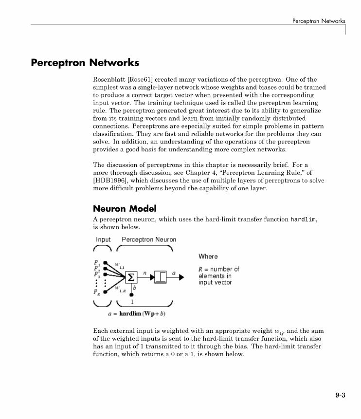
Perceptron Networks
Perceptron NetworksRosenblatt [Rose61] created many variations of the perceptron. One of thesimplest was a single-layer network whose weights and biases could be trainedto produce a correct target vector when presented with the correspondinginput vector. The training technique used is called the perceptron learningrule. The perceptron generated great interest due to its ability to generalizefrom its training vectors and learn from initially randomly distributedconnections. Perceptrons are especially suited for simple problems in patternclassification. They are fast and reliable networks for the problems they cansolve. In addition, an understanding of the operations of the perceptronprovides a good basis for understanding more complex networks.
The discussion of perceptrons in this chapter is necessarily brief. For amore thorough discussion, see Chapter 4, “Perceptron Learning Rule,” of[HDB1996], which discusses the use of multiple layers of perceptrons to solvemore difficult problems beyond the capability of one layer.
Neuron ModelA perceptron neuron, which uses the hard-limit transfer function hardlim,is shown below.
Each external input is weighted with an appropriate weight w1j, and the sumof the weighted inputs is sent to the hard-limit transfer function, which alsohas an input of 1 transmitted to it through the bias. The hard-limit transferfunction, which returns a 0 or a 1, is shown below.
9-3
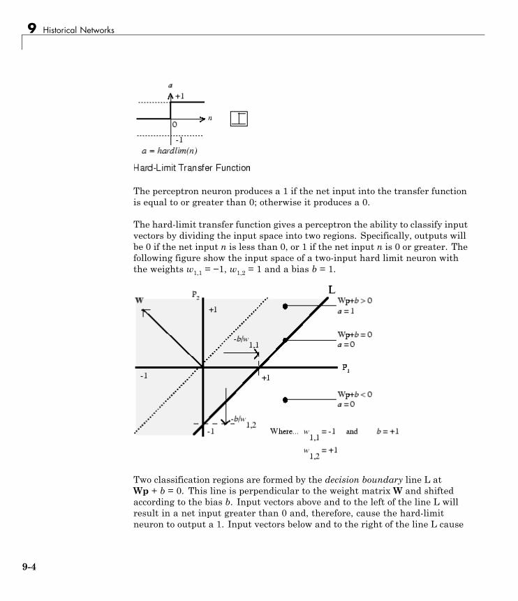
9 Historical Networks
The perceptron neuron produces a 1 if the net input into the transfer functionis equal to or greater than 0; otherwise it produces a 0.
The hard-limit transfer function gives a perceptron the ability to classify inputvectors by dividing the input space into two regions. Specifically, outputs willbe 0 if the net input n is less than 0, or 1 if the net input n is 0 or greater. Thefollowing figure show the input space of a two-input hard limit neuron withthe weights w1,1 = −1, w1,2 = 1 and a bias b = 1.
Two classification regions are formed by the decision boundary line L atWp + b = 0. This line is perpendicular to the weight matrix W and shiftedaccording to the bias b. Input vectors above and to the left of the line L willresult in a net input greater than 0 and, therefore, cause the hard-limitneuron to output a 1. Input vectors below and to the right of the line L cause
9-4
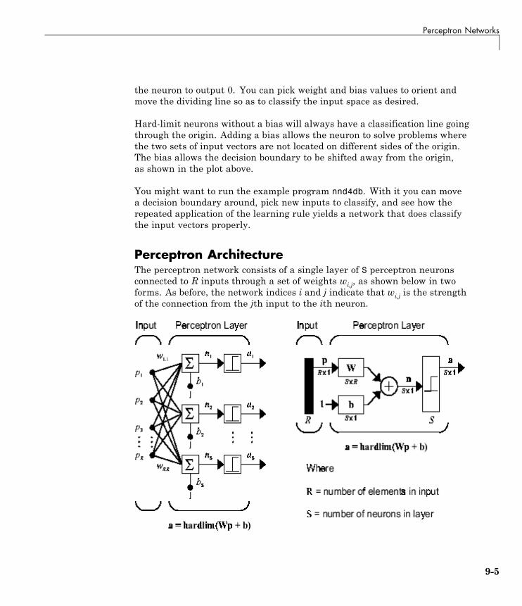
Perceptron Networks
the neuron to output 0. You can pick weight and bias values to orient andmove the dividing line so as to classify the input space as desired.
Hard-limit neurons without a bias will always have a classification line goingthrough the origin. Adding a bias allows the neuron to solve problems wherethe two sets of input vectors are not located on different sides of the origin.The bias allows the decision boundary to be shifted away from the origin,as shown in the plot above.
You might want to run the example program nnd4db. With it you can movea decision boundary around, pick new inputs to classify, and see how therepeated application of the learning rule yields a network that does classifythe input vectors properly.
Perceptron ArchitectureThe perceptron network consists of a single layer of S perceptron neuronsconnected to R inputs through a set of weights wi,j, as shown below in twoforms. As before, the network indices i and j indicate that wi,j is the strengthof the connection from the jth input to the ith neuron.
9-5
9 Historical Networks
The perceptron learning rule described shortly is capable of training onlya single layer. Thus only one-layer networks are considered here. Thisrestriction places limitations on the computation a perceptron can perform.The types of problems that perceptrons are capable of solving are discussed in“Limitations and Cautions” on page 9-16.
Create a PerceptronYou can create a perceptron with the following:
net = perceptron;net = configure(net,P,T);
where input arguments are as follows:
• P is an R-by-Q matrix of Q input vectors of R elements each.
• T is an S-by-Q matrix of Q target vectors of S elements each.
Commonly, the hardlim function is used in perceptrons, so it is the default.
The following commands create a perceptron network with a singleone-element input vector with the values 0 and 2, and one neuron withoutputs that can be either 0 or 1:
P = [0 2];T = [0 1];net = perceptron;net = configure(net,P,T);
You can see what network has been created by executing the followingcommand:
inputweights = net.inputweights{1,1}
which yields
inputweights =delays: 0
initFcn: 'initzero'learn: true
9-6
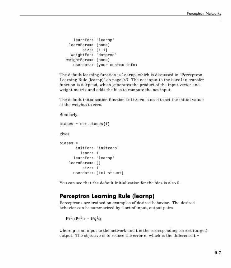
Perceptron Networks
learnFcn: 'learnp'learnParam: (none)
size: [1 1]weightFcn: 'dotprod'
weightParam: (none)userdata: (your custom info)
The default learning function is learnp, which is discussed in “PerceptronLearning Rule (learnp)” on page 9-7. The net input to the hardlim transferfunction is dotprod, which generates the product of the input vector andweight matrix and adds the bias to compute the net input.
The default initialization function initzero is used to set the initial valuesof the weights to zero.
Similarly,
biases = net.biases{1}
gives
biases =initFcn: 'initzero'
learn: 1learnFcn: 'learnp'
learnParam: []size: 1
userdata: [1x1 struct]
You can see that the default initialization for the bias is also 0.
Perceptron Learning Rule (learnp)Perceptrons are trained on examples of desired behavior. The desiredbehavior can be summarized by a set of input, output pairs
p t p t p t1 1 2 1, , , Q Q
where p is an input to the network and t is the corresponding correct (target)output. The objective is to reduce the error e, which is the difference t −
9-7
9 Historical Networks
a between the neuron response a and the target vector t. The perceptronlearning rule learnp calculates desired changes to the perceptron’s weightsand biases, given an input vector p and the associated error e. The targetvector t must contain values of either 0 or 1, because perceptrons (withhardlim transfer functions) can only output these values.
Each time learnp is executed, the perceptron has a better chance of producingthe correct outputs. The perceptron rule is proven to converge on a solution ina finite number of iterations if a solution exists.
If a bias is not used, learnp works to find a solution by altering only theweight vector w to point toward input vectors to be classified as 1 and awayfrom vectors to be classified as 0. This results in a decision boundary that isperpendicular to w and that properly classifies the input vectors.
There are three conditions that can occur for a single neuron once an inputvector p is presented and the network’s response a is calculated:
CASE 1. If an input vector is presented and the output of the neuron iscorrect (a = t and e = t – a = 0), then the weight vector w is not altered.
CASE 2. If the neuron output is 0 and should have been 1 (a = 0 and t = 1,and e = t – a = 1), the input vector p is added to the weight vector w. Thismakes the weight vector point closer to the input vector, increasing the chancethat the input vector will be classified as a 1 in the future.
CASE 3. If the neuron output is 1 and should have been 0 (a = 1 and t = 0, ande = t – a = –1), the input vector p is subtracted from the weight vector w. Thismakes the weight vector point farther away from the input vector, increasingthe chance that the input vector will be classified as a 0 in the future.
The perceptron learning rule can be written more succinctly in terms of theerror e = t – a and the change to be made to the weight vector Δw:
CASE 1. If e = 0, then make a change Δw equal to 0.
CASE 2. If e = 1, then make a change Δw equal to pT.
CASE 3. If e = –1, then make a change Δw equal to –pT.
9-8
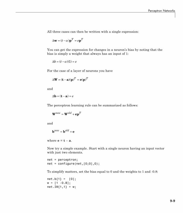
Perceptron Networks
All three cases can then be written with a single expression:
Δw p p= − =( )t eT T
You can get the expression for changes in a neuron’s bias by noting that thebias is simply a weight that always has an input of 1:
Δb t e= − =( )( ) 1
For the case of a layer of neurons you have
ΔW t a p e p= − =( )( ) ( )T T
and
Δb t a= − =( ) e
The perceptron learning rule can be summarized as follows:
W W epnew old T= +
and
b b enew old= +
where e = t – a.
Now try a simple example. Start with a single neuron having an input vectorwith just two elements.
net = perceptron;net = configure(net,[0;0],0);
To simplify matters, set the bias equal to 0 and the weights to 1 and -0.8:
net.b{1} = [0];w = [1 -0.8];net.IW{1,1} = w;
9-9
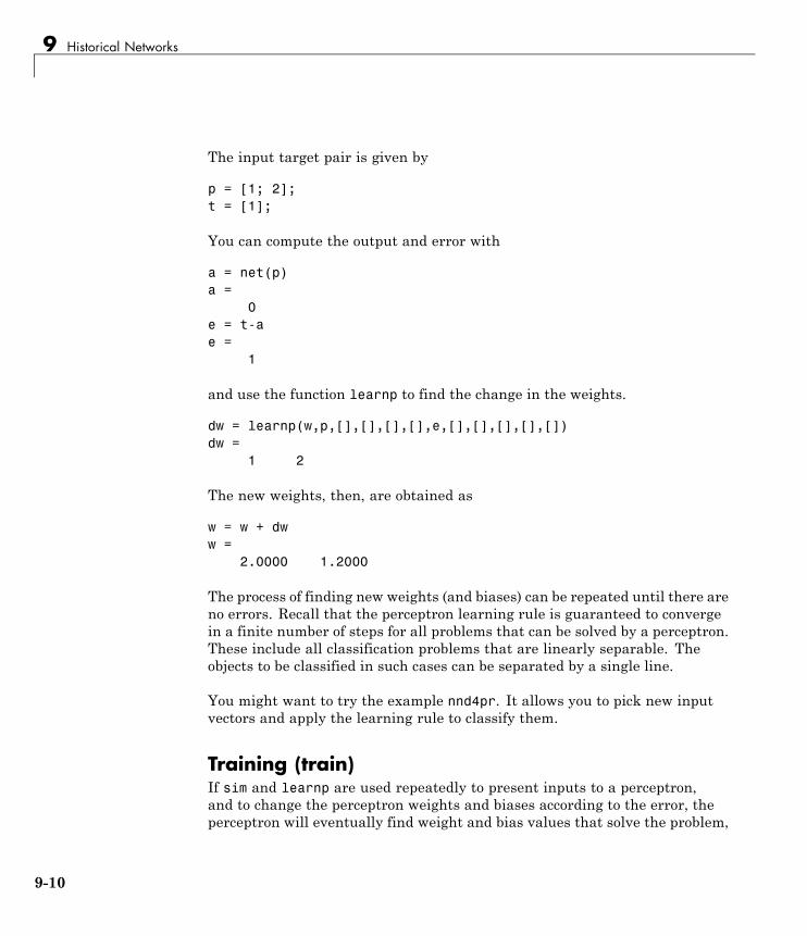
9 Historical Networks
The input target pair is given by
p = [1; 2];t = [1];
You can compute the output and error with
a = net(p)a =
0e = t-ae =
1
and use the function learnp to find the change in the weights.
dw = learnp(w,p,[],[],[],[],e,[],[],[],[],[])dw =
1 2
The new weights, then, are obtained as
w = w + dww =
2.0000 1.2000
The process of finding new weights (and biases) can be repeated until there areno errors. Recall that the perceptron learning rule is guaranteed to convergein a finite number of steps for all problems that can be solved by a perceptron.These include all classification problems that are linearly separable. Theobjects to be classified in such cases can be separated by a single line.
You might want to try the example nnd4pr. It allows you to pick new inputvectors and apply the learning rule to classify them.
Training (train)If sim and learnp are used repeatedly to present inputs to a perceptron,and to change the perceptron weights and biases according to the error, theperceptron will eventually find weight and bias values that solve the problem,
9-10
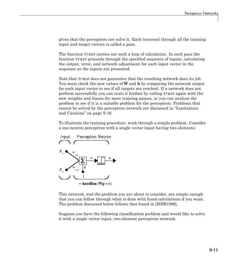
Perceptron Networks
given that the perceptron can solve it. Each traversal through all the traininginput and target vectors is called a pass.
The function train carries out such a loop of calculation. In each pass thefunction train proceeds through the specified sequence of inputs, calculatingthe output, error, and network adjustment for each input vector in thesequence as the inputs are presented.
Note that train does not guarantee that the resulting network does its job.You must check the new values ofW and b by computing the network outputfor each input vector to see if all targets are reached. If a network does notperform successfully you can train it further by calling train again with thenew weights and biases for more training passes, or you can analyze theproblem to see if it is a suitable problem for the perceptron. Problems thatcannot be solved by the perceptron network are discussed in “Limitationsand Cautions” on page 9-16.
To illustrate the training procedure, work through a simple problem. Considera one-neuron perceptron with a single vector input having two elements:
This network, and the problem you are about to consider, are simple enoughthat you can follow through what is done with hand calculations if you want.The problem discussed below follows that found in [HDB1996].
Suppose you have the following classification problem and would like to solveit with a single vector input, two-element perceptron network.
9-11
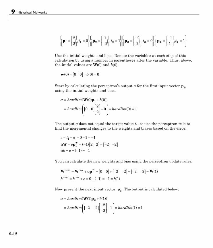
9 Historical Networks
p p p1 1 2 2 322
012
12
2
, ,t t
, ,t t3 4 40
11
1p
Use the initial weights and bias. Denote the variables at each step of thiscalculation by using a number in parentheses after the variable. Thus, above,the initial values are W(0) and b(0).
w( ) ( )0 0 0 0 0= [ ] =b
Start by calculating the perceptron’s output a for the first input vector p1,using the initial weights and bias.
= +
= [ ]⎡
⎣⎢
⎤
⎦⎥ +
⎛
⎝⎜
⎞
⎠⎟ =
hardlim b
hardlim hardlim
( ( ) ( ))W p0 0
0 022
0
1
(( )0 1=
The output a does not equal the target value t1, so use the perceptron rule tofind the incremental changes to the weights and biases based on the error.
e t
e
b e
T
= − = − = −
= = − [ ] = − −[ ]= = − = −
1
1
0 1 1
1 2 2 2 2
1 1
ΔΔ
W p ( )
( )
You can calculate the new weights and bias using the perceptron update rules.
W W ep Wnew old T
new oldb b e
= + = [ ] + − −[ ] = − −[ ] =
= + = + − = −
0 0 2 2 2 2 1
0 1 1
( )
( ) == b( )1
Now present the next input vector, p2. The output is calculated below.
= +
= − −[ ] −−
⎡
⎣⎢
⎤
⎦⎥ −
⎛
⎝⎜
⎞
⎠⎟ =
hardlim b
hardlim har
( ( ) ( ))W p1 1
2 222
1
2
ddlim( )1 1=
9-12
Perceptron Networks
On this occasion, the target is 1, so the error is zero. Thus there are nochanges in weights or bias, soW(2) =W(1) = [−2 −2] and p(2) = p(1) = −1.
You can continue in this fashion, presenting p3 next, calculating an outputand the error, and making changes in the weights and bias, etc. After makingone pass through all of the four inputs, you get the valuesW(4) = [−3 −1] andb(4) = 0. To determine whether a satisfactory solution is obtained, make onepass through all input vectors to see if they all produce the desired targetvalues. This is not true for the fourth input, but the algorithm does convergeon the sixth presentation of an input. The final values are
W(6) = [−2 −3] and b(6) = 1.
This concludes the hand calculation. Now, how can you do this using thetrain function?
The following code defines a perceptron.
net = perceptron;
Consider the application of a single input
p = [2; 2];
having the target
t = [0];
Set epochs to 1, so that train goes through the input vectors (only one here)just one time.
net.trainParam.epochs = 1;net = train(net,p,t);
The new weights and bias are
w = net.iw{1,1}, b = net.b{1}w =
-2 -2b =
-1
9-13
9 Historical Networks
Thus, the initial weights and bias are 0, and after training on only the firstvector, they have the values [−2 −2] and −1, just as you hand calculated.
Now apply the second input vector p2. The output is 1, as it will be until theweights and bias are changed, but now the target is 1, the error will be 0, andthe change will be zero. You could proceed in this way, starting from theprevious result and applying a new input vector time after time. But you cando this job automatically with train.
Apply train for one epoch, a single pass through the sequence of all fourinput vectors. Start with the network definition.
net = perceptron;net.trainParam.epochs = 1;
The input vectors and targets are
p = [[2;2] [1;-2] [-2;2] [-1;1]]t = [0 1 0 1]
Now train the network with
net = train(net,p,t);
The new weights and bias are
w = net.iw{1,1}, b = net.b{1}w =
-3 -1b =
0
This is the same result as you got previously by hand.
Finally, simulate the trained network for each of the inputs.
a = net(p)a =
0 0 1 1
9-14
Perceptron Networks
The outputs do not yet equal the targets, so you need to train the network formore than one pass. Try more epochs. This run gives a mean absolute errorperformance of 0 after two epochs:
net.trainParam.epochs = 1000;net = train(net,p,t);
Thus, the network was trained by the time the inputs were presented on thethird epoch. (As you know from hand calculation, the network converges onthe presentation of the sixth input vector. This occurs in the middle of thesecond epoch, but it takes the third epoch to detect the network convergence.)The final weights and bias are
w = net.iw{1,1}, b = net.b{1}w =
-2 -3b =
1
The simulated output and errors for the various inputs are
a = net(p)a =
0 1 0 1error = a-terror =
0 0 0 0
You confirm that the training procedure is successful. The network convergesand produces the correct target outputs for the four input vectors.
The default training function for networks created with newp is trainc. (Youcan find this by executing net.trainFcn.) This training function applies theperceptron learning rule in its pure form, in that individual input vectors areapplied individually, in sequence, and corrections to the weights and bias aremade after each presentation of an input vector. Thus, perceptron trainingwith train will converge in a finite number of steps unless the problempresented cannot be solved with a simple perceptron.
9-15
9 Historical Networks
The function train can be used in various ways by other networks as well.Type help train to read more about this basic function.
You might want to try various example programs. For instance, demop1illustrates classification and training of a simple perceptron.
Limitations and CautionsPerceptron networks should be trained with adapt, which presents theinput vectors to the network one at a time and makes corrections to thenetwork based on the results of each presentation. Use of adapt in this wayguarantees that any linearly separable problem is solved in a finite number oftraining presentations.
As noted in the previous pages, perceptrons can also be trained with thefunction train. Commonly when train is used for perceptrons, it presentsthe inputs to the network in batches, and makes corrections to the networkbased on the sum of all the individual corrections. Unfortunately, there isno proof that such a training algorithm converges for perceptrons. On thataccount the use of train for perceptrons is not recommended.
Perceptron networks have several limitations. First, the output valuesof a perceptron can take on only one of two values (0 or 1) because of thehard-limit transfer function. Second, perceptrons can only classify linearlyseparable sets of vectors. If a straight line or a plane can be drawn to separatethe input vectors into their correct categories, the input vectors are linearlyseparable. If the vectors are not linearly separable, learning will never reacha point where all vectors are classified properly. However, it has been proventhat if the vectors are linearly separable, perceptrons trained adaptively willalways find a solution in finite time. You might want to try demop6. It showsthe difficulty of trying to classify input vectors that are not linearly separable.
It is only fair, however, to point out that networks with more than oneperceptron can be used to solve more difficult problems. For instance, supposethat you have a set of four vectors that you would like to classify into distinctgroups, and that two lines can be drawn to separate them. A two-neuronnetwork can be found such that its two decision boundaries classify the inputsinto four categories. For additional discussion about perceptrons and toexamine more complex perceptron problems, see [HDB1996].
9-16
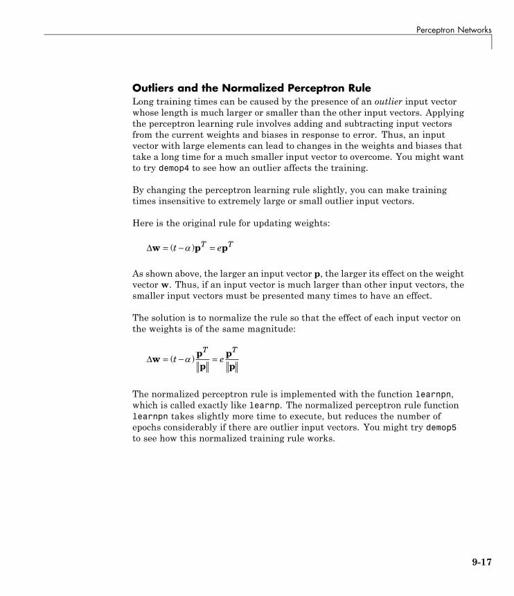
Perceptron Networks
Outliers and the Normalized Perceptron RuleLong training times can be caused by the presence of an outlier input vectorwhose length is much larger or smaller than the other input vectors. Applyingthe perceptron learning rule involves adding and subtracting input vectorsfrom the current weights and biases in response to error. Thus, an inputvector with large elements can lead to changes in the weights and biases thattake a long time for a much smaller input vector to overcome. You might wantto try demop4 to see how an outlier affects the training.
By changing the perceptron learning rule slightly, you can make trainingtimes insensitive to extremely large or small outlier input vectors.
Here is the original rule for updating weights:
Δw p p= − =( )t eT T
As shown above, the larger an input vector p, the larger its effect on the weightvector w. Thus, if an input vector is much larger than other input vectors, thesmaller input vectors must be presented many times to have an effect.
The solution is to normalize the rule so that the effect of each input vector onthe weights is of the same magnitude:
Δwpp
pp
= − =( )t eT T
The normalized perceptron rule is implemented with the function learnpn,which is called exactly like learnp. The normalized perceptron rule functionlearnpn takes slightly more time to execute, but reduces the number ofepochs considerably if there are outlier input vectors. You might try demop5to see how this normalized training rule works.
9-17
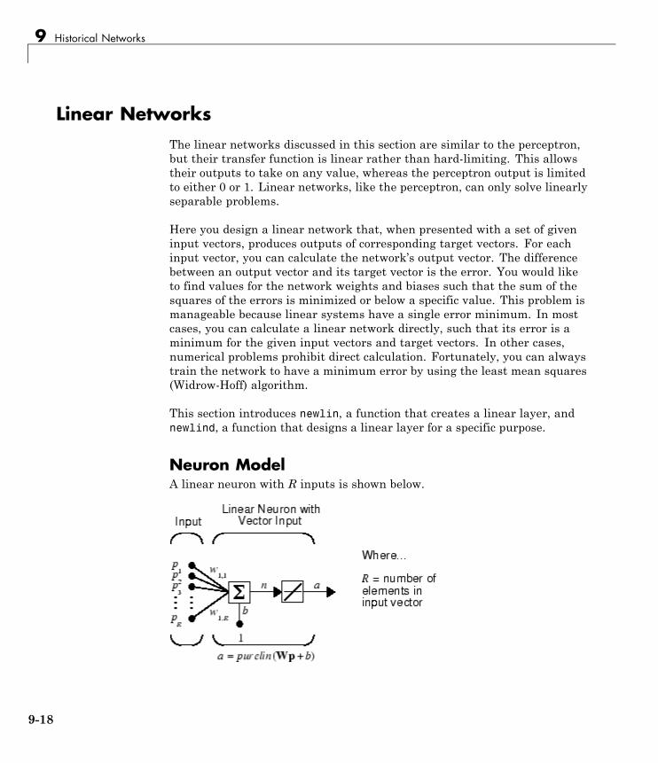
9 Historical Networks
Linear NetworksThe linear networks discussed in this section are similar to the perceptron,but their transfer function is linear rather than hard-limiting. This allowstheir outputs to take on any value, whereas the perceptron output is limitedto either 0 or 1. Linear networks, like the perceptron, can only solve linearlyseparable problems.
Here you design a linear network that, when presented with a set of giveninput vectors, produces outputs of corresponding target vectors. For eachinput vector, you can calculate the network’s output vector. The differencebetween an output vector and its target vector is the error. You would liketo find values for the network weights and biases such that the sum of thesquares of the errors is minimized or below a specific value. This problem ismanageable because linear systems have a single error minimum. In mostcases, you can calculate a linear network directly, such that its error is aminimum for the given input vectors and target vectors. In other cases,numerical problems prohibit direct calculation. Fortunately, you can alwaystrain the network to have a minimum error by using the least mean squares(Widrow-Hoff) algorithm.
This section introduces newlin, a function that creates a linear layer, andnewlind, a function that designs a linear layer for a specific purpose.
Neuron ModelA linear neuron with R inputs is shown below.
9-18
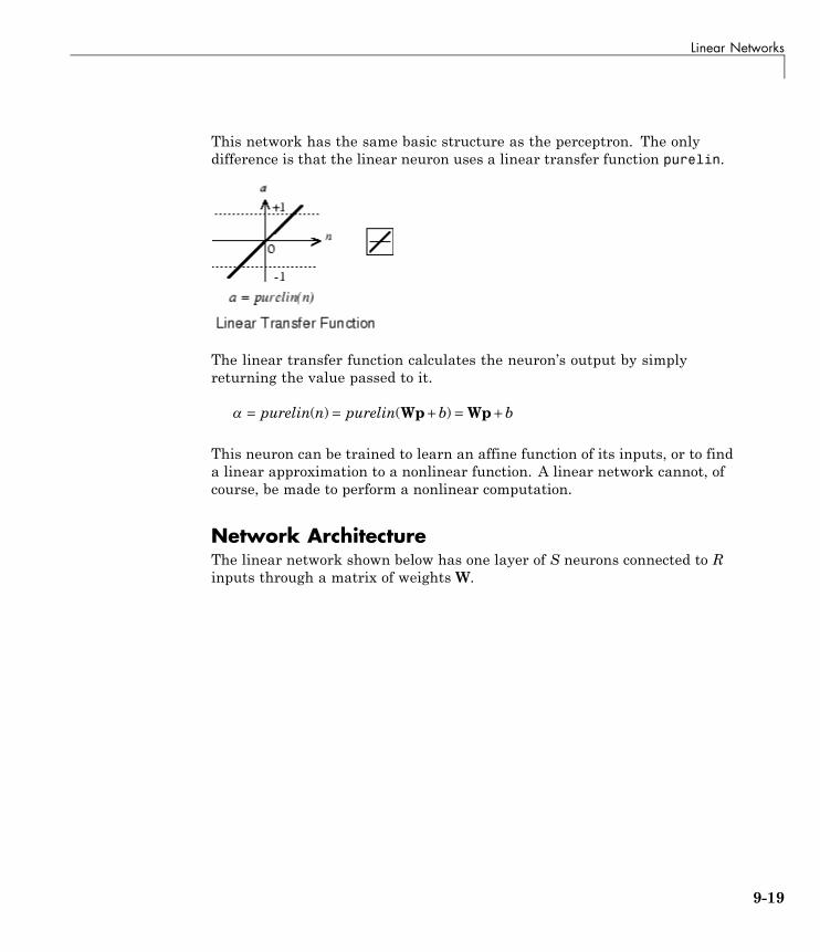
Linear Networks
This network has the same basic structure as the perceptron. The onlydifference is that the linear neuron uses a linear transfer function purelin.
The linear transfer function calculates the neuron’s output by simplyreturning the value passed to it.
= = + = +purelin n purelin b b( ) ( )Wp Wp
This neuron can be trained to learn an affine function of its inputs, or to finda linear approximation to a nonlinear function. A linear network cannot, ofcourse, be made to perform a nonlinear computation.
Network ArchitectureThe linear network shown below has one layer of S neurons connected to Rinputs through a matrix of weights W.
9-19
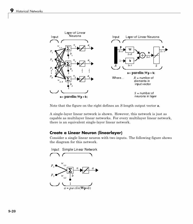
9 Historical Networks
Note that the figure on the right defines an S-length output vector a.
A single-layer linear network is shown. However, this network is just ascapable as multilayer linear networks. For every multilayer linear network,there is an equivalent single-layer linear network.
Create a Linear Neuron (linearlayer)Consider a single linear neuron with two inputs. The following figure showsthe diagram for this network.
9-20
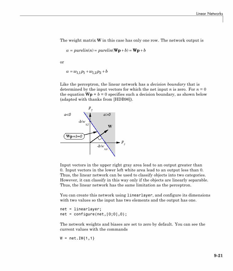
Linear Networks
The weight matrixW in this case has only one row. The network output is
= = + = +purelin n purelin b b( ) ( )Wp Wp
or
= + +w p w p b1 1 1 1 2 2, ,
Like the perceptron, the linear network has a decision boundary that isdetermined by the input vectors for which the net input n is zero. For n = 0the equation Wp + b = 0 specifies such a decision boundary, as shown below(adapted with thanks from [HDB96]).
Input vectors in the upper right gray area lead to an output greater than0. Input vectors in the lower left white area lead to an output less than 0.Thus, the linear network can be used to classify objects into two categories.However, it can classify in this way only if the objects are linearly separable.Thus, the linear network has the same limitation as the perceptron.
You can create this network using linearlayer, and configure its dimensionswith two values so the input has two elements and the output has one.
net = linearlayer;net = configure(net,[0;0],0);
The network weights and biases are set to zero by default. You can see thecurrent values with the commands
W = net.IW{1,1}
9-21
9 Historical Networks
W =0 0
and
b= net.b{1}b =
0
However, you can give the weights any values that you want, such as 2 and3, respectively, with
net.IW{1,1} = [2 3];W = net.IW{1,1}W =
2 3
You can set and check the bias in the same way.
net.b{1} = [-4];b = net.b{1}b =
-4
You can simulate the linear network for a particular input vector. Try
p = [5;6];
You can find the network output with the function sim.
a = net(p)a =
24
To summarize, you can create a linear network with newlin, adjust itselements as you want, and simulate it with sim. You can find more aboutnewlin by typing help newlin.
9-22

Linear Networks
Least Mean Square ErrorLike the perceptron learning rule, the least mean square error (LMS)algorithm is an example of supervised training, in which the learning rule isprovided with a set of examples of desired network behavior:
p t p t p t1 1 2 2, , , , ,{ } { } { } Q Q
Here pq is an input to the network, and tq is the corresponding target output.As each input is applied to the network, the network output is comparedto the target. The error is calculated as the difference between the targetoutput and the network output. The goal is to minimize the average of thesum of these errors.
mseQ
e kQ
t k kk
Q
k
Q= = −
= =∑ ∑1 12
1
2
1
( ) ( ( ) ( ))
The LMS algorithm adjusts the weights and biases of the linear network so asto minimize this mean square error.
Fortunately, the mean square error performance index for the linear networkis a quadratic function. Thus, the performance index will either have oneglobal minimum, a weak minimum, or no minimum, depending on thecharacteristics of the input vectors. Specifically, the characteristics of theinput vectors determine whether or not a unique solution exists.
You can find more about this topic in Chapter 10 of [HDB96].
Linear System Design (newlind)Unlike most other network architectures, linear networks can be designeddirectly if input/target vector pairs are known. You can obtain specificnetwork values for weights and biases to minimize the mean square error byusing the function newlind.
Suppose that the inputs and targets are
P = [1 2 3];T= [2.0 4.1 5.9];
9-23
9 Historical Networks
Now you can design a network.
net = newlind(P,T);
You can simulate the network behavior to check that the design was doneproperly.
Y = net(P)Y =
2.0500 4.0000 5.9500
Note that the network outputs are quite close to the desired targets.
You might try demolin1. It shows error surfaces for a particular problem,illustrates the design, and plots the designed solution.
You can also use the function newlind to design linear networks havingdelays in the input. Such networks are discussed in “Linear Networks withDelays” on page 9-24. First, however, delays must be discussed.
Linear Networks with Delays
Tapped Delay LineYou need a new component, the tapped delay line, to make full use of thelinear network. Such a delay line is shown below. There the input signalenters from the left and passes through N-1 delays. The output of the tappeddelay line (TDL) is an N-dimensional vector, made up of the input signal atthe current time, the previous input signal, etc.
9-24
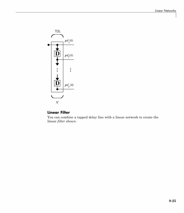
Linear Networks
Linear FilterYou can combine a tapped delay line with a linear network to create thelinear filter shown.
9-25
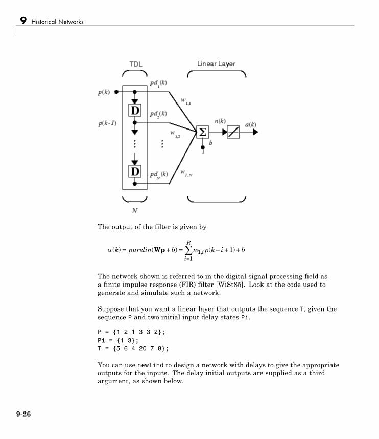
9 Historical Networks
The output of the filter is given by
( ) ( ) ( ),k purelin b w p k i bii
R= + = − + +
=∑Wp 1
1
1
The network shown is referred to in the digital signal processing field asa finite impulse response (FIR) filter [WiSt85]. Look at the code used togenerate and simulate such a network.
Suppose that you want a linear layer that outputs the sequence T, given thesequence P and two initial input delay states Pi.
P = {1 2 1 3 3 2};Pi = {1 3};T = {5 6 4 20 7 8};
You can use newlind to design a network with delays to give the appropriateoutputs for the inputs. The delay initial outputs are supplied as a thirdargument, as shown below.
9-26
Linear Networks
net = newlind(P,T,Pi);
You can obtain the output of the designed network with
Y = net(P,Pi)
to give
Y = [2.7297] [10.5405] [5.0090] [14.9550] [10.7838] [5.9820]
As you can see, the network outputs are not exactly equal to the targets, butthey are close and the mean square error is minimized.
LMS Algorithm (learnwh)The LMS algorithm, or Widrow-Hoff learning algorithm, is based on anapproximate steepest descent procedure. Here again, linear networks aretrained on examples of correct behavior.
Widrow and Hoff had the insight that they could estimate the mean squareerror by using the squared error at each iteration. If you take the partialderivative of the squared error with respect to the weights and biases at thekth iteration, you have
∂∂
= ∂∂
e kw
e ke kwj j
2
1 12
( )( )
( )
, ,
for j = 1,2,…,R and
∂∂
= ∂∂
e kb
e ke kb
22
( )( )
( )
Next look at the partial derivative with respect to the error.
∂∂
= ∂ −∂
= ∂∂
− +e kw
t k kw w
t k k bj j j
( ) [ ( ) ( )][ ( ) ( ( ) )]
, , ,1 1 1
Wp
or
9-27
9 Historical Networks
∂∂
= ∂∂
− +⎛
⎝⎜⎜
⎞
⎠⎟⎟
⎡
⎣⎢⎢
⎤
⎦⎥⎥=
∑e kw w
t k w p k bj j
i ii
R( )( ) ( )
, ,,
1 11
1
Here pi(k) is the ith element of the input vector at the kth iteration.
This can be simplified to
∂∂
= −e kw
p kj
j( )
( ),1
and
∂∂
= −e kb( )
1
Finally, change the weight matrix, and the bias will be
2αe(k)p(k)
and
2αe(k)
These two equations form the basis of the Widrow-Hoff (LMS) learningalgorithm.
These results can be extended to the case of multiple neurons, and writtenin matrix form as
W W e pb b e
( ) ( ) ( ) ( )( ) ( ) ( )
k k k kk k k
T+ = ++ = +
1 21 2
Here the error e and the bias b are vectors, and α is a learning rate. If α islarge, learning occurs quickly, but if it is too large it can lead to instabilityand errors might even increase. To ensure stable learning, the learning ratemust be less than the reciprocal of the largest eigenvalue of the correlationmatrix pTp of the input vectors.
9-28
Linear Networks
You might want to read some of Chapter 10 of [HDB96] for more informationabout the LMS algorithm and its convergence.
Fortunately, there is a toolbox function, learnwh, that does all the calculationfor you. It calculates the change in weights as
dw = lr*e*p'
and the bias change as
db = lr*e
The constant 2, shown a few lines above, has been absorbed into the codelearning rate lr. The function maxlinlr calculates this maximum stablelearning rate lr as 0.999 * P'*P.
Type help learnwh and help maxlinlr for more details about these twofunctions.
Linear Classification (train)Linear networks can be trained to perform linear classification with thefunction train. This function applies each vector of a set of input vectorsand calculates the network weight and bias increments due to each of theinputs according to learnp. Then the network is adjusted with the sum ofall these corrections. Each pass through the input vectors is called an epoch.This contrasts with adapt which adjusts weights for each input vector as itis presented.
Finally, train applies the inputs to the new network, calculates the outputs,compares them to the associated targets, and calculates a mean square error.If the error goal is met, or if the maximum number of epochs is reached,the training is stopped, and train returns the new network and a trainingrecord. Otherwise train goes through another epoch. Fortunately, the LMSalgorithm converges when this procedure is executed.
A simple problem illustrates this procedure. Consider the linear networkintroduced earlier.
9-29
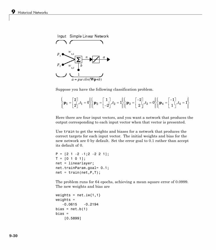
9 Historical Networks
Suppose you have the following classification problem.
p p p1 1 2 2 322
012
12
2
, ,t t
, ,t t3 4 40
11
1p
Here there are four input vectors, and you want a network that produces theoutput corresponding to each input vector when that vector is presented.
Use train to get the weights and biases for a network that produces thecorrect targets for each input vector. The initial weights and bias for thenew network are 0 by default. Set the error goal to 0.1 rather than acceptits default of 0.
P = [2 1 -2 -1;2 -2 2 1];T = [0 1 0 1];net = linearlayer;net.trainParam.goal= 0.1;net = train(net,P,T);
The problem runs for 64 epochs, achieving a mean square error of 0.0999.The new weights and bias are
weights = net.iw{1,1}weights =
-0.0615 -0.2194bias = net.b(1)bias =
[0.5899]
9-30
Linear Networks
You can simulate the new network as shown below.
A = net(P)A =
0.0282 0.9672 0.2741 0.4320
You can also calculate the error.
err = T - sim(net,P)err =
-0.0282 0.0328 -0.2741 0.5680
Note that the targets are not realized exactly. The problem would have runlonger in an attempt to get perfect results had a smaller error goal beenchosen, but in this problem it is not possible to obtain a goal of 0. The networkis limited in its capability. See “Limitations and Cautions” on page 9-31 forexamples of various limitations.
This example program, demolin2, shows the training of a linear neuron andplots the weight trajectory and error during training.
You might also try running the example program nnd10lc. It addresses aclassic and historically interesting problem, shows how a network can betrained to classify various patterns, and shows how the trained networkresponds when noisy patterns are presented.
Limitations and CautionsLinear networks can only learn linear relationships between input and outputvectors. Thus, they cannot find solutions to some problems. However, even ifa perfect solution does not exist, the linear network will minimize the sumof squared errors if the learning rate lr is sufficiently small. The networkwill find as close a solution as is possible given the linear nature of thenetwork’s architecture. This property holds because the error surface of alinear network is a multidimensional parabola. Because parabolas have onlyone minimum, a gradient descent algorithm (such as the LMS rule) mustproduce a solution at that minimum.
9-31
9 Historical Networks
Linear networks have various other limitations. Some of them are discussedbelow.
Overdetermined SystemsConsider an overdetermined system. Suppose that you have a network tobe trained with four one-element input vectors and four targets. A perfectsolution to wp + b = t for each of the inputs might not exist, for there are fourconstraining equations, and only one weight and one bias to adjust. However,the LMS rule still minimizes the error. You might try demolin4 to see howthis is done.
Underdetermined SystemsConsider a single linear neuron with one input. This time, in demolin5, trainit on only one one-element input vector and its one-element target vector:
P = [1.0];T = [0.5];
Note that while there is only one constraint arising from the singleinput/target pair, there are two variables, the weight and the bias. Havingmore variables than constraints results in an underdetermined problem withan infinite number of solutions. You can try demolin5 to explore this topic.
Linearly Dependent VectorsNormally it is a straightforward job to determine whether or not a linearnetwork can solve a problem. Commonly, if a linear network has at leastas many degrees of freedom (S *R + S = number of weights and biases) asconstraints (Q = pairs of input/target vectors), then the network can solve theproblem. This is true except when the input vectors are linearly dependentand they are applied to a network without biases. In this case, as shownwith the example demolin6, the network cannot solve the problem with zeroerror. You might want to try demolin6.
Too Large a Learning RateYou can always train a linear network with the Widrow-Hoff rule to find theminimum error solution for its weights and biases, as long as the learningrate is small enough. Example demolin7 shows what happens when a
9-32

Linear Networks
neuron with one input and a bias is trained with a learning rate larger thanthat recommended by maxlinlr. The network is trained with two differentlearning rates to show the results of using too large a learning rate.
9-33
9 Historical Networks
Hopfield Network
FundamentalsThe goal here is to design a network that stores a specific set of equilibriumpoints such that, when an initial condition is provided, the network eventuallycomes to rest at such a design point. The network is recursive in that theoutput is fed back as the input, once the network is in operation. Hopefully,the network output will settle on one of the original design points.
The design method presented is not perfect in that the designed network canhave spurious undesired equilibrium points in addition to the desired ones.However, the number of these undesired points is made as small as possibleby the design method. Further, the domain of attraction of the designedequilibrium points is as large as possible.
The design method is based on a system of first-order linear ordinarydifferential equations that are defined on a closed hypercube of the statespace. The solutions exist on the boundary of the hypercube. These systemshave the basic structure of the Hopfield model, but are easier to understandand design than the Hopfield model.
The material in this section is based on the following paper: Jian-Hua Li,Anthony N. Michel, and Wolfgang Porod, “Analysis and synthesis of a classof neural networks: linear systems operating on a closed hypercube,” IEEETrans. on Circuits and Systems, Vol. 36, No. 11, November 1989, pp. 1405–22.
For further information on Hopfield networks, read Chapter 18 of theHopfield Network [HDB96].
ArchitectureThe architecture of the Hopfield network follows.
9-34
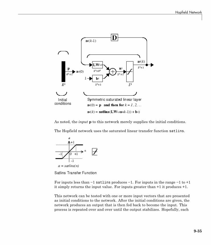
Hopfield Network
As noted, the input p to this network merely supplies the initial conditions.
The Hopfield network uses the saturated linear transfer function satlins.
For inputs less than −1 satlins produces −1. For inputs in the range −1 to +1it simply returns the input value. For inputs greater than +1 it produces +1.
This network can be tested with one or more input vectors that are presentedas initial conditions to the network. After the initial conditions are given, thenetwork produces an output that is then fed back to become the input. Thisprocess is repeated over and over until the output stabilizes. Hopefully, each
9-35
9 Historical Networks
output vector eventually converges to one of the design equilibrium pointvectors that is closest to the input that provoked it.
Design (newhop)Li et al. [LiMi89] have studied a system that has the basic structure of theHopfield network but is, in Li’s own words, “easier to analyze, synthesize, andimplement than the Hopfield model.” The authors are enthusiastic aboutthe reference article, as it has many excellent points and is one of the mostreadable in the field. However, the design is mathematically complex, andeven a short justification of it would burden this guide. Thus the Li designmethod is presented, with thanks to Li et al., as a recipe that is found inthe function newhop.
Given a set of target equilibrium points represented as a matrix T of vectors,newhop returns weights and biases for a recursive network. The network isguaranteed to have stable equilibrium points at the target vectors, but itcould contain other spurious equilibrium points as well. The number of theseundesired points is made as small as possible by the design method.
Once the network has been designed, it can be tested with one or more inputvectors. Hopefully those input vectors close to target equilibrium points willfind their targets. As suggested by the network figure, an array of inputvectors is presented one at a time or in a batch. The network proceeds to giveoutput vectors that are fed back as inputs. These output vectors can be can becompared to the target vectors to see how the solution is proceeding.
The ability to run batches of trial input vectors quickly allows you to checkthe design in a relatively short time. First you might check to see that thetarget equilibrium point vectors are indeed contained in the network. Thenyou could try other input vectors to determine the domains of attraction of thetarget equilibrium points and the locations of spurious equilibrium points ifthey are present.
Consider the following design example. Suppose that you want to design anetwork with two stable points in a three-dimensional space.
T = [-1 -1 1; 1 -1 1]'T =
-1 1
9-36
Hopfield Network
-1 -11 1
You can execute the design with
net = newhop(T);
Next, check to make sure that the designed network is at these two points,as follows. Because Hopfield networks have no inputs, the second argumentto the network is an empty cell array whose columns indicate the numberof time steps.
Ai = {T};[Y,Pf,Af] = net(cell(1,2),{},Ai);Y{2}
This gives you
-1 1-1 -11 1
Thus, the network has indeed been designed to be stable at its design points.Next you can try another input condition that is not a design point, such as
Ai = {[-0.9; -0.8; 0.7]};
This point is reasonably close to the first design point, so you might anticipatethat the network would converge to that first point. To see if this happens,run the following code.
[Y,Pf,Af] = net(cell(1,5),{},Ai);Y{end}
This produces
-1-11
Thus, an original condition close to a design point did converge to that point.
9-37
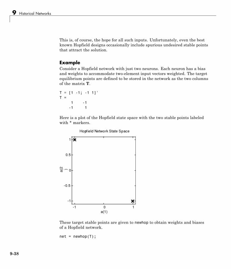
9 Historical Networks
This is, of course, the hope for all such inputs. Unfortunately, even the bestknown Hopfield designs occasionally include spurious undesired stable pointsthat attract the solution.
ExampleConsider a Hopfield network with just two neurons. Each neuron has a biasand weights to accommodate two-element input vectors weighted. The targetequilibrium points are defined to be stored in the network as the two columnsof the matrix T.
T = [1 -1; -1 1]'T =
1 -1-1 1
Here is a plot of the Hopfield state space with the two stable points labeledwith * markers.
These target stable points are given to newhop to obtain weights and biasesof a Hopfield network.
net = newhop(T);
9-38
Hopfield Network
The design returns a set of weights and a bias for each neuron. The resultsare obtained from
W = net.LW{1,1}
which gives
W =0.6925 -0.4694
-0.4694 0.6925
and from
b = net.b{1,1}
which gives
b =00
Next test the design with the target vectors T to see if they are stored in thenetwork. The targets are used as inputs for the simulation function sim.
Ai = {T};[Y,Pf,Af] = net(cell(1,2),{},Ai);Y = Y{end}ans =
1 -1-1 1
As hoped, the new network outputs are the target vectors. The solution staysat its initial conditions after a single update and, therefore, will stay therefor any number of updates.
Now you might wonder how the network performs with various random inputvectors. Here is a plot showing the paths that the network took through itsstate space to arrive at a target point.
9-39
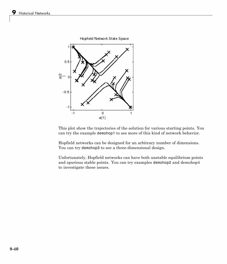
9 Historical Networks
This plot show the trajectories of the solution for various starting points. Youcan try the example demohop1 to see more of this kind of network behavior.
Hopfield networks can be designed for an arbitrary number of dimensions.You can try demohop3 to see a three-dimensional design.
Unfortunately, Hopfield networks can have both unstable equilibrium pointsand spurious stable points. You can try examples demohop2 and demohop4to investigate these issues.
9-40
Summary
SummaryHopfield networks can act as error correction or vector categorizationnetworks. Input vectors are used as the initial conditions to the network,which recurrently updates until it reaches a stable output vector.
Hopfield networks are interesting from a theoretical standpoint, but areseldom used in practice. Even the best Hopfield designs may have spuriousstable points that lead to incorrect answers. More efficient and reliable errorcorrection techniques, such as backpropagation, are available.
FunctionsThis chapter introduces the following functions:
Function Description
newhop Create a Hopfield recurrent network.
satlins Symmetric saturating linear transfer function.
9-41

9 Historical Networks
9-42

10
Network Object Reference
• “Network Properties” on page 10-2
• “Subobject Properties” on page 10-15
10 Network Object Reference
Network PropertiesThese properties define the basic features of a network. “Subobject Properties”on page 10-15 describes properties that define network details.
GeneralHere are the general properties of neural networks.
net.nameThis property consists of a string defining the network name. Networkcreation functions, such as feedforwardnet, define this appropriately. But itcan be set to any string as desired.
net.userdataThis property provides a place for users to add custom information to anetwork object. Only one field is predefined. It contains a secret message toall Neural Network Toolbox users:
net.userdata.note
EfficiencyHere are the efficiency properties of neural networks.
net.efficiency.cacheDelayedInputThis property can be set to true (the default) or false. If true then the delayedinputs of each input weight are calculated once during training and reused,instead of recalculated each time they are needed. This results in fastertraining, but at the expense of memory efficiency. For greater memoryefficiency set this property to false.
net.efficiency.flattenTimeThis property can be set to true (the default) or false. If true then time seriesdata used to train static networks will be reformatted as static data beforetraining. This results in faster training at the expense of memory efficiency.
10-2
Network Properties
For greater memory efficiency, either only use static data for static networks,or set this property to false.
net.efficiency.memoryReductionThis property can be set to 1 (the default) or any integer greater than 1. If setto an integer N, then simulation and error gradient and Jacobian calculationswill be split in time into N subcalculations by groups of samples. This willresult in greater time overhead but result in reduced memory requirementsfor storing intermediate values. For greater memory efficiency, set this tohigher values.
ArchitectureThese properties determine the number of network subobjects (which includeinputs, layers, outputs, targets, biases, and weights), and how they areconnected.
net.numInputsThis property defines the number of inputs a network receives. It can beset to 0 or a positive integer.
Clarification. The number of network inputs and the size of a networkinput are not the same thing. The number of inputs defines how many setsof vectors the network receives as input. The size of each input (i.e., thenumber of elements in each input vector) is determined by the input size(net.inputs{i}.size).
Most networks have only one input, whose size is determined by the problem.
Side Effects. Any change to this property results in a change in the size ofthe matrix defining connections to layers from inputs, (net.inputConnect)and the size of the cell array of input subobjects (net.inputs).
net.numLayersThis property defines the number of layers a network has. It can be set to 0or a positive integer.
10-3

10 Network Object Reference
Side Effects. Any change to this property changes the size of each of theseBoolean matrices that define connections to and from layers:
net.biasConnectnet.inputConnectnet.layerConnectnet.outputConnect
and changes the size of each cell array of subobject structures whose sizedepends on the number of layers:
net.biasesnet.inputWeightsnet.layerWeightsnet.outputs
and also changes the size of each of the network’s adjustable parameter’sproperties:
net.IWnet.LWnet.b
net.biasConnectThis property defines which layers have biases. It can be set to any N-by-1matrix of Boolean values, where Nl is the number of network layers(net.numLayers). The presence (or absence) of a bias to the ith layer isindicated by a 1 (or 0) at
net.biasConnect(i)
Side Effects. Any change to this property alters the presence or absence ofstructures in the cell array of biases (net.biases) and, in the presence orabsence of vectors in the cell array, of bias vectors (net.b).
net.inputConnectThis property defines which layers have weights coming from inputs.
10-4
Network Properties
It can be set to any Nl × Ni matrix of Boolean values, where Nl is the numberof network layers (net.numLayers), and Ni is the number of network inputs(net.numInputs). The presence (or absence) of a weight going to the ith layerfrom the jth input is indicated by a 1 (or 0) at net.inputConnect(i,j).
Side Effects. Any change to this property alters the presence or absence ofstructures in the cell array of input weight subobjects (net.inputWeights)and the presence or absence of matrices in the cell array of input weightmatrices (net.IW).
net.layerConnectThis property defines which layers have weights coming from other layers. Itcan be set to any Nl × Nl matrix of Boolean values, where Nl is the number ofnetwork layers (net.numLayers). The presence (or absence) of a weight goingto the ith layer from the jth layer is indicated by a 1 (or 0) at
net.layerConnect(i,j)
Side Effects. Any change to this property alters the presence or absence ofstructures in the cell array of layer weight subobjects (net.layerWeights)and the presence or absence of matrices in the cell array of layer weightmatrices (net.LW).
net.outputConnectThis property defines which layers generate network outputs. It can be set toany 1 × Nlmatrix of Boolean values, where Nl is the number of network layers(net.numLayers). The presence (or absence) of a network output from the ithlayer is indicated by a 1 (or 0) at net.outputConnect(i).
Side Effects. Any change to this property alters the number of networkoutputs (net.numOutputs) and the presence or absence of structures in thecell array of output subobjects (net.outputs).
net.numOutputs (read only)This property indicates how many outputs the network has. It is always equalto the number of 1s in net.outputConnect.
10-5
10 Network Object Reference
net.numInputDelays (read only)This property indicates the number of time steps of past inputs that must besupplied to simulate the network. It is always set to the maximum delayvalue associated with any of the network’s input weights:
numInputDelays = 0;for i=1:net.numLayers
for j=1:net.numInputsif net.inputConnect(i,j)
numInputDelays = max( ...[numInputDelays net.inputWeights{i,j}.delays]);
endend
end
net.numLayerDelays (read only)This property indicates the number of time steps of past layer outputs thatmust be supplied to simulate the network. It is always set to the maximumdelay value associated with any of the network’s layer weights:
numLayerDelays = 0;for i=1:net.numLayers
for j=1:net.numLayersif net.layerConnect(i,j)
numLayerDelays = max( ...[numLayerDelays net.layerWeights{i,j}.delays]);
endend
end
net.numWeightElements (read only)This property indicates the number of weight and bias values in the network.It is the sum of the number of elements in the matrices stored in the twocell arrays:
net.IWnew.b
10-6
Network Properties
Subobject StructuresThese properties consist of cell arrays of structures that define each of thenetwork’s inputs, layers, outputs, targets, biases, and weights.
The properties for each kind of subobject are described in “SubobjectProperties” on page 10-15.
net.inputsThis property holds structures of properties for each of the network’s inputs.It is always an Ni × 1 cell array of input structures, where Ni is the numberof network inputs (net.numInputs).
The structure defining the properties of the ith network input is located at
net.inputs{i}
Input Properties. See “Inputs” on page 10-15 for descriptions of inputproperties.
net.layersThis property holds structures of properties for each of the network’s layers.It is always an Nl × 1 cell array of layer structures, where Nl is the numberof network layers (net.numLayers).
The structure defining the properties of the ith layer is located atnet.layers{i}.
Layer Properties. See “Layers” on page 10-17 for descriptions of layerproperties.
net.outputsThis property holds structures of properties for each of the network’s outputs.It is always a 1 × Nl cell array, where Nl is the number of network outputs(net.numOutputs).
10-7
10 Network Object Reference
The structure defining the properties of the output from the ith layer (or a nullmatrix []) is located at net.outputs{i} if net.outputConnect(i) is 1 (or 0).
Output Properties. See “Outputs” on page 10-23 for descriptions of outputproperties.
net.biasesThis property holds structures of properties for each of the network’s biases.It is always an Nl × 1 cell array, where Nl is the number of network layers(net.numLayers).
The structure defining the properties of the bias associated with the ith layer(or a null matrix []) is located at net.biases{i} if net.biasConnect(i) is1 (or 0).
Bias Properties. See “Biases” on page 10-25 for descriptions of biasproperties.
net.inputWeightsThis property holds structures of properties for each of the network’s inputweights. It is always an Nl × Ni cell array, where Nl is the number ofnetwork layers (net.numLayers), and Ni is the number of network inputs(net.numInputs).
The structure defining the properties of the weight going to the ith layer fromthe jth input (or a null matrix []) is located at net.inputWeights{i,j} ifnet.inputConnect(i,j) is 1 (or 0).
Input Weight Properties. See “Input Weights” on page 10-26 fordescriptions of input weight properties.
net.layerWeightsThis property holds structures of properties for each of the network’s layerweights. It is always an Nl ×Nl cell array, where Nl is the number of networklayers (net.numLayers).
10-8
Network Properties
The structure defining the properties of the weight going to the ith layer fromthe jth layer (or a null matrix []) is located at net.layerWeights{i,j} ifnet.layerConnect(i,j) is 1 (or 0).
Layer Weight Properties. See “Layer Weights” on page 10-28 fordescriptions of layer weight properties.
FunctionsThese properties define the algorithms to use when a network is to adapt, isto be initialized, is to have its performance measured, or is to be trained.
net.adaptFcnThis property defines the function to be used when the network adapts. It canbe set to the name of any network adapt function. The network adapt functionis used to perform adaption whenever adapt is called.
[net,Y,E,Pf,Af] = adapt(NET,P,T,Pi,Ai)
For a list of functions, type help nntrain.
Side Effects. Whenever this property is altered, the network’s adaptionparameters (net.adaptParam) are set to contain the parameters and defaultvalues of the new function.
net.adaptParamThis property defines the parameters and values of the current adaptfunction. Call help on the current adapt function to get a description of whateach field means:
help(net.adaptFcn)
net.derivFcnThis property defines the derivative function to be used to calculate errorgradients and Jacobians when the network is trained using a supervisedalgorithm, such as backpropagation. You can set this property to the name ofany derivative function.
10-9

10 Network Object Reference
For a list of functions, type help nnderivative.
net.divideFcnThis property defines the data division function to be used when the networkis trained using a supervised algorithm, such as backpropagation. You can setthis property to the name of a division function.
For a list of functions, type help nndivision.
Side Effects. Whenever this property is altered, the network’s adaptionparameters (net.divideParam) are set to contain the parameters and defaultvalues of the new function.
net.divideParamThis property defines the parameters and values of the current data-divisionfunction. To get a description of what each field means, type the followingcommand:
help(net.divideParam)
net.divideModeThis property defines the target data dimensions which to divide up whenthe data division function is called. Its default value is 'sample' forstatic networks and 'time' for dynamic networks. It may also be set to'sampletime' to divide targets by both sample and timestep, 'all' to divideup targets by every scalar value, or 'none' to not divide up data at all (inwhich case all data is used for training, none for validation or testing).
net.initFcnThis property defines the function used to initialize the network’s weightmatrices and bias vectors. . The initialization function is used to initializethe network whenever init is called:
net = init(net)
10-10
Network Properties
Side Effects. Whenever this property is altered, the network’s initializationparameters (net.initParam) are set to contain the parameters and defaultvalues of the new function.
net.initParamThis property defines the parameters and values of the current initializationfunction. Call help on the current initialization function to get a descriptionof what each field means:
help(net.initFcn)
net.performFcnThis property defines the function used to measure the network’s performance.The performance function is used to calculate network performance duringtraining whenever train is called.
[net,tr] = train(NET,P,T,Pi,Ai)
For a list of functions, type help nnperformance.
Side Effects. Whenever this property is altered, the network’s performanceparameters (net.performParam) are set to contain the parameters anddefault values of the new function.
net.performParamThis property defines the parameters and values of the current performancefunction. Call help on the current performance function to get a description ofwhat each field means:
help(net.performFcn)
net.plotFcnsThis property consists of a row cell array of strings, defining the plot functionsassociated with a network. The neural network training window, which isopened by the train function, shows a button for each plotting function. Clickthe button during or after training to open the desired plot.
10-11
10 Network Object Reference
net.plotParamsThis property consists of a row cell array of structures, defining theparameters and values of each plot function in net.plotFcns. Call help onthe each plot function to get a description of what each field means:
help(net.plotFcns{i})
net.trainFcnThis property defines the function used to train the network. It can be set tothe name of any of the “Fitting Functions and Data”. The training function isused to train the network whenever train is called.
[net,tr] = train(NET,P,T,Pi,Ai)
For a list of functions, type help nntrain.
Side Effects. Whenever this property is altered, the network’s trainingparameters (net.trainParam) are set to contain the parameters and defaultvalues of the new function.
net.trainParamThis property defines the parameters and values of the current trainingfunction. Call help on the current training function to get a description ofwhat each field means:
help(net.trainFcn)
Weight and Bias ValuesThese properties define the network’s adjustable parameters: its weightmatrices and bias vectors.
net.IWThis property defines the weight matrices of weights going to layers fromnetwork inputs. It is always an Nl × Ni cell array, where Nl is the numberof network layers (net.numLayers), and Ni is the number of network inputs(net.numInputs).
10-12
Network Properties
The weight matrix for the weight going to the ith layer from the jth input (ora null matrix []) is located at net.IW{i,j} if net.inputConnect(i,j) is1 (or 0).
The weight matrix has as many rows as the size of the layer it goes to(net.layers{i}.size). It has as many columns as the product of the inputsize with the number of delays associated with the weight:
net.inputs{j}.size * length(net.inputWeights{i,j}.delays)
These dimensions can also be obtained from the input weight properties:
net.inputWeights{i,j}.size
net.LWThis property defines the weight matrices of weights going to layers fromother layers. It is always an Nl × Nl cell array, where Nl is the number ofnetwork layers (net.numLayers).
The weight matrix for the weight going to the ith layer from the jth layer (ora null matrix []) is located at net.LW{i,j} if net.layerConnect(i,j) is1 (or 0).
The weight matrix has as many rows as the size of the layer it goes to(net.layers{i}.size). It has as many columns as the product of the size ofthe layer it comes from with the number of delays associated with the weight:
net.layers{j}.size * length(net.layerWeights{i,j}.delays)
These dimensions can also be obtained from the layer weight properties:
net.layerWeights{i,j}.size
net.bThis property defines the bias vectors for each layer with a bias. It is always anNl × 1 cell array, where Nl is the number of network layers (net.numLayers).
10-13

10 Network Object Reference
The bias vector for the ith layer (or a null matrix []) is located at net.b{i}if net.biasConnect(i) is 1 (or 0).
The number of elements in the bias vector is always equal to the size of thelayer it is associated with (net.layers{i}.size).
This dimension can also be obtained from the bias properties:
net.biases{i}.size
10-14
Subobject Properties
Subobject PropertiesThese properties define the details of a network’s inputs, layers, outputs,targets, biases, and weights.
InputsThese properties define the details of each ith network input.
net.inputs{1}.nameThis property consists of a string defining the input name. Network creationfunctions, such as feedforwardnet, define this appropriately. But it can beset to any string as desired.
net.inputs{i}.feedbackInput (read only)If this network is associated with an open-loop feedback output, then thisproperty will indicate the index of that output. Otherwise it will be an emptymatrix.
net.inputs{i}.processFcnsThis property defines a row cell array of processing function names to be usedby ith network input. The processing functions are applied to input valuesbefore the network uses them.
Side Effects. Whenever this property is altered, the input processParamsare set to default values for the given processing functions, processSettings,processedSize, and processedRange are defined by applying the processfunctions and parameters to exampleInput.
For a list of processing functions, type help nnprocess.
net.inputs{i}.processParamsThis property holds a row cell array of processing function parameters to beused by ith network input. The processing parameters are applied by theprocessing functions to input values before the network uses them.
10-15
10 Network Object Reference
Side Effects. Whenever this property is altered, the input processSettings,processedSize, and processedRange are defined by applying the processfunctions and parameters to exampleInput.
net.inputs{i}.processSettings (read only)This property holds a row cell array of processing function settings to beused by ith network input. The processing settings are found by applyingthe processing functions and parameters to exampleInput and then used toprovide consistent results to new input values before the network uses them.
net.inputs{i}.processedRange (read only)This property defines the range of exampleInput values after they have beenprocessed with processingFcns and processingParams.
net.inputs{i}.processedSize (read only)This property defines the number of rows in the exampleInput values afterthey have been processed with processingFcns and processingParams.
net.inputs{i}.rangeThis property defines the range of each element of the ith network input.
It can be set to any Ri × 2 matrix, where Ri is the number of elements inthe input (net.inputs{i}.size), and each element in column 1 is less thanthe element next to it in column 2.
Each jth row defines the minimum and maximum values of the jth inputelement, in that order:
net.inputs{i}(j,:)
Uses. Some initialization functions use input ranges to find appropriateinitial values for input weight matrices.
Side Effects. Whenever the number of rows in this property is altered,the input size, processedSize, and processedRange change to remainconsistent. The sizes of any weights coming from this input and thedimensions of the weight matrices also change.
10-16
Subobject Properties
net.inputs{i}.sizeThis property defines the number of elements in the ith network input. Itcan be set to 0 or a positive integer.
Side Effects. Whenever this property is altered, the input range,processedRange, and processedSize are updated. Any associated inputweights change size accordingly.
net.inputs{i}.userdataThis property provides a place for users to add custom information to theith network input.
LayersThese properties define the details of each ith network layer.
net.layers{i}.nameThis property consists of a string defining the layer name. Network creationfunctions, such as feedforwardnet, define this appropriately. But it can beset to any string as desired.
net.layers{i}.dimensionsThis property defines the physical dimensions of the ith layer’s neurons.Being able to arrange a layer’s neurons in a multidimensional manner isimportant for self-organizing maps.
It can be set to any row vector of 0 or positive integer elements, where theproduct of all the elements becomes the number of neurons in the layer(net.layers{i}.size).
Uses. Layer dimensions are used to calculate the neuron positions withinthe layer (net.layers{i}.positions) using the layer’s topology function(net.layers{i}.topologyFcn).
10-17
10 Network Object Reference
Side Effects. Whenever this property is altered, the layer’s size(net.layers{i}.size) changes to remain consistent. The layer’s neuronpositions (net.layers{i}.positions) and the distances between the neurons(net.layers{i}.distances) are also updated.
net.layers{i}.distanceFcnThis property defines which of the distance functions is used to calculatedistances between neurons in the ith layer from the neuron positions.Neuron distances are used by self-organizing maps. It can be set to the nameof any distance function.
For a list of functions, type help nndistance.
Side Effects. Whenever this property is altered, the distances between thelayer’s neurons (net.layers{i}.distances) are updated.
net.layers{i}.distances (read only)This property defines the distances between neurons in the ith layer. Thesedistances are used by self-organizing maps:
net.layers{i}.distances
It is always set to the result of applying the layer’s distance function(net.layers{i}.distanceFcn) to the positions of the layer’s neurons(net.layers{i}.positions).
net.layers{i}.initFcnThis property defines which of the layer initialization functions are used toinitialize the ith layer, if the network initialization function (net.initFcn)is initlay. If the network initialization is set to initlay, then the functionindicated by this property is used to initialize the layer’s weights and biases.
net.layers{i}.netInputFcnThis property defines which of the net input functions is used to calculatethe ith layer’s net input, given the layer’s weighted inputs and bias duringsimulating and training.
10-18

Subobject Properties
For a list of functions, type help nnnetinput.
net.layers{i}.netInputParamThis property defines the parameters of the layer’s net input function. Callhelp on the current net input function to get a description of each field:
help(net.layers{i}.netInputFcn)
net.layers{i}.positions (read only)This property defines the positions of neurons in the ith layer. These positionsare used by self-organizing maps.
It is always set to the result of applying the layer’s topology function(net.layers{i}.topologyFcn) to the positions of the layer’s dimensions(net.layers{i}.dimensions).
Plotting. Use plotsom to plot the positions of a layer’s neurons.
For instance, if the first-layer neurons of a network are arranged withdimensions (net.layers{1}.dimensions) of [4 5], and the topology function(net.layers{1}.topologyFcn) is hextop, the neurons’ positions can beplotted as follows:
plotsom(net.layers{1}.positions)
10-19
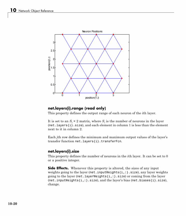
10 Network Object Reference
net.layers{i}.range (read only)This property defines the output range of each neuron of the ith layer.
It is set to an Si × 2 matrix, where Si is the number of neurons in the layer(net.layers{i}.size), and each element in column 1 is less than the elementnext to it in column 2.
Each jth row defines the minimum and maximum output values of the layer’stransfer function net.layers{i}.transferFcn.
net.layers{i}.sizeThis property defines the number of neurons in the ith layer. It can be set to 0or a positive integer.
Side Effects. Whenever this property is altered, the sizes of any inputweights going to the layer (net.inputWeights{i,:}.size), any layer weightsgoing to the layer (net.layerWeights{i,:}.size) or coming from the layer(net.inputWeights{i,:}.size), and the layer’s bias (net.biases{i}.size),change.
10-20
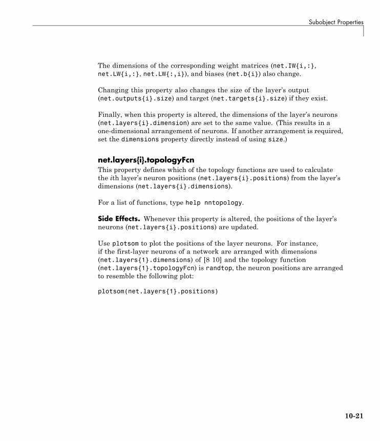
Subobject Properties
The dimensions of the corresponding weight matrices (net.IW{i,:},net.LW{i,:}, net.LW{:,i}), and biases (net.b{i}) also change.
Changing this property also changes the size of the layer’s output(net.outputs{i}.size) and target (net.targets{i}.size) if they exist.
Finally, when this property is altered, the dimensions of the layer’s neurons(net.layers{i}.dimension) are set to the same value. (This results in aone-dimensional arrangement of neurons. If another arrangement is required,set the dimensions property directly instead of using size.)
net.layers{i}.topologyFcnThis property defines which of the topology functions are used to calculatethe ith layer’s neuron positions (net.layers{i}.positions) from the layer’sdimensions (net.layers{i}.dimensions).
For a list of functions, type help nntopology.
Side Effects. Whenever this property is altered, the positions of the layer’sneurons (net.layers{i}.positions) are updated.
Use plotsom to plot the positions of the layer neurons. For instance,if the first-layer neurons of a network are arranged with dimensions(net.layers{1}.dimensions) of [8 10] and the topology function(net.layers{1}.topologyFcn) is randtop, the neuron positions are arrangedto resemble the following plot:
plotsom(net.layers{1}.positions)
10-21
10 Network Object Reference
net.layers{i}.transferFcnThis function defines which of the transfer functions is used to calculate theith layer’s output, given the layer’s net input, during simulation and training.
For a list of functions, type help nntransfer.
net.layers{i}.transferParamThis property defines the parameters of the layer’s transfer function. Callhelp on the current transfer function to get a description of what each fieldmeans:
help(net.layers{i}.transferFcn)
net.layers{i}.userdataThis property provides a place for users to add custom information to theith network layer.
10-22
Subobject Properties
Outputs
net.outputs{i}.nameThis property consists of a string defining the output name. Network creationfunctions, such as feedforwardnet, define this appropriately. But it can beset to any string as desired.
net.outputs{i}.feedbackInputIf the output implements open-loop feedback (net.outputs{i}.feedbackMode= 'open'), then this property indicates the index of the associated feedbackinput, otherwise it will be an empty matrix.
net.outputs{i}.feedbackDelayThis property defines the timestep difference between this output andnetwork inputs. Input-to-output network delays can be removed and addedwith removedelay and adddelay functions resulting in this property beingincremented or decremented respectively. The difference in timing betweeninputs and outputs is used by preparets to properly format simulation andtraining data, and used by closeloop to add the correct number of delayswhen closing an open-loop output, and openloop to remove delays whenopening a closed loop.
net.outputs{i}.feedbackModeThis property is set to the string 'none' for non-feedback outputs. Forfeedback outputs it can either be set to 'open' or 'closed'. If it is set to'open', then the output will be associated with a feedback input, with theproperty feedbackInput indicating the input’s index.
net.outputs{i}.processFcnsThis property defines a row cell array of processing function names to be usedby the ith network output. The processing functions are applied to targetvalues before the network uses them, and applied in reverse to layer outputvalues before being returned as network output values.
10-23
10 Network Object Reference
Side Effects. When you change this property, you also affect the followingsettings: the output parameters processParams are modified to thedefault values of the specified processing functions; processSettings,processedSize, and processedRange are defined using the results ofapplying the process functions and parameters to exampleOutput; the ithlayer size is updated to match the processedSize.
For a list of functions, type help nnprocess.
net.outputs{i}.processParamsThis property holds a row cell array of processing function parameters to beused by ith network output on target values. The processing parametersare applied by the processing functions to input values before the networkuses them.
Side Effects. Whenever this property is altered, the output processSettings,processedSize and processedRange are defined by applying the processfunctions and parameters to exampleOutput. The ith layer’s size is alsoupdated to match processedSize.
net.outputs{i}.processSettings (read only)This property holds a row cell array of processing function settings to be usedby ith network output. The processing settings are found by applying theprocessing functions and parameters to exampleOutput and then used toprovide consistent results to new target values before the network uses them.The processing settings are also applied in reverse to layer output valuesbefore being returned by the network.
net.outputs{i}.processedRange (read only)This property defines the range of exampleOutput values after they have beenprocessed with processingFcns and processingParams.
net.outputs{i}.processedSize (read only)This property defines the number of rows in the exampleOutput values afterthey have been processed with processingFcns and processingParams.
10-24

Subobject Properties
net.outputs{i}.size (read only)This property defines the number of elements in the ith layer’s output. It isalways set to the size of the ith layer (net.layers{i}.size).
net.outputs{i}.userdataThis property provides a place for users to add custom information to theith layer’s output.
Biases
net.biases{i}.initFcnThis property defines the weight and bias initialization functions used to setthe ith layer’s bias vector (net.b{i}) if the network initialization function isinitlay and the ith layer’s initialization function is initwb.
net.biases{i}.learnThis property defines whether the ith bias vector is to be altered duringtraining and adaption. It can be set to 0 or 1.
It enables or disables the bias’s learning during calls to adapt and train.
net.biases{i}.learnFcnThis property defines which of the learning functions is used to update theith layer’s bias vector (net.b{i}) during training, if the network trainingfunction is trainb, trainc, or trainr, or during adaption, if the networkadapt function is trains.
For a list of functions, type help nnlearn.
Side Effects. Whenever this property is altered, the biases learningparameters (net.biases{i}.learnParam) are set to contain the fields anddefault values of the new function.
10-25
10 Network Object Reference
net.biases{i}.learnParamThis property defines the learning parameters and values for the currentlearning function of the ith layer’s bias. The fields of this property depend onthe current learning function. Call help on the current learning function toget a description of what each field means.
net.biases{i}.size (read only)This property defines the size of the ith layer’s bias vector. It is always setto the size of the ith layer (net.layers{i}.size).
net.biases{i}.userdataThis property provides a place for users to add custom information to theith layer’s bias.
Input Weights
net.inputWeights{i,j}.delaysThis property defines a tapped delay line between the jth input and its weightto the ith layer. It must be set to a row vector of increasing values. Theelements must be either 0 or positive integers.
Side Effects. Whenever this property is altered, the weight’s size(net.inputWeights{i,j}.size) and the dimensions of its weight matrix(net.IW{i,j}) are updated.
net.inputWeights{i,j}.initFcnThis property defines which of the Weight and Bias Initialization Functions isused to initialize the weight matrix (net.IW{i,j}) going to the ith layer fromthe jth input, if the network initialization function is initlay, and the ithlayer’s initialization function is initwb. This function can be set to the nameof any weight initialization function.
10-26
Subobject Properties
net.inputWeights{i,j}.initSettings (read only)This property is set to values useful for initializing the weight as part of theconfiguration process that occurs automatically the first time a network istrained, or when the function configure is called on a network directly.
net.inputWeights{i,j}.learnThis property defines whether the weight matrix to the ith layer from the jthinput is to be altered during training and adaption. It can be set to 0 or 1.
net.inputWeights{i,j}.learnFcnThis property defines which of the learning functions is used to update theweight matrix (net.IW{i,j}) going to the ith layer from the jth input duringtraining, if the network training function is trainb, trainc, or trainr, orduring adaption, if the network adapt function is trains. It can be set to thename of any weight learning function.
For a list of functions, type help nnlearn.
net.inputWeights{i,j}.learnParamThis property defines the learning parameters and values for the currentlearning function of the ith layer’s weight coming from the jth input.
The fields of this property depend on the current learning function(net.inputWeights{i,j}.learnFcn). Evaluate the above reference to see thefields of the current learning function.
Call help on the current learning function to get a description of what eachfield means.
net.inputWeights{i,j}.size (read only)This property defines the dimensions of the ith layer’s weight matrix from thejth network input. It is always set to a two-element row vector indicating thenumber of rows and columns of the associated weight matrix (net.IW{i,j}).The first element is equal to the size of the ith layer (net.layers{i}.size).The second element is equal to the product of the length of the weight’s delayvectors and the size of the jth input:
10-27
10 Network Object Reference
length(net.inputWeights{i,j}.delays) * net.inputs{j}.size
net.inputWeights{i,j}.userdataThis property provides a place for users to add custom information to the(i,j)th input weight.
net.inputWeights{i,j}.weightFcnThis property defines which of the weight functions is used to apply the ithlayer’s weight from the jth input to that input. It can be set to the name ofany weight function. The weight function is used to transform layer inputsduring simulation and training.
For a list of functions, type help nnweight.
net.inputWeights{i,j}.weightParamThis property defines the parameters of the layer’s net input function. Callhelp on the current net input function to get a description of each field.
Layer Weights
net.layerWeights{i,j}.delaysThis property defines a tapped delay line between the jth layer and its weightto the ith layer. It must be set to a row vector of increasing values. Theelements must be either 0 or positive integers.
net.layerWeights{i,j}.initFcnThis property defines which of the weight and bias initialization functions isused to initialize the weight matrix (net.LW{i,j}) going to the ith layer fromthe jth layer, if the network initialization function is initlay, and the ithlayer’s initialization function is initwb. This function can be set to the nameof any weight initialization function.
10-28
Subobject Properties
net.layerWeights{i,j}.initSettings (read only)This property is set to values useful for initializing the weight as part of theconfiguration process that occurs automatically the first time a network istrained, or when the function configure is called on a network directly.
net.layerWeights{i,j}.learnThis property defines whether the weight matrix to the ith layer from the jthlayer is to be altered during training and adaption. It can be set to 0 or 1.
net.layerWeights{i,j}.learnFcnThis property defines which of the learning functions is used to update theweight matrix (net.LW{i,j}) going to the ith layer from the jth layer duringtraining, if the network training function is trainb, trainc, or trainr, orduring adaption, if the network adapt function is trains. It can be set to thename of any weight learning function.
For a list of functions, type help nnlearn.
net.layerWeights{i,j}.learnParamThis property defines the learning parameters fields and values for thecurrent learning function of the ith layer’s weight coming from the jth layer.The fields of this property depend on the current learning function. Call helpon the current net input function to get a description of each field.
net.layerWeights{i,j}.size (read only)This property defines the dimensions of the ith layer’s weight matrix from thejth layer. It is always set to a two-element row vector indicating the numberof rows and columns of the associated weight matrix (net.LW{i,j}). Thefirst element is equal to the size of the ith layer (net.layers{i}.size). Thesecond element is equal to the product of the length of the weight’s delayvectors and the size of the jth layer.
net.layerWeights{i,j}.userdataThis property provides a place for users to add custom information to the(i,j)th layer weight.
10-29

10 Network Object Reference
net.layerWeights{i,j}.weightFcnThis property defines which of the weight functions is used to apply the ithlayer’s weight from the jth layer to that layer’s output. It can be set to thename of any weight function. The weight function is used to transform layerinputs when the network is simulated.
For a list of functions, type help nnweight.
net.layerWeights{i,j}.weightParamThis property defines the parameters of the layer’s net input function. Callhelp on the current net input function to get a description of each field.
10-30

11
Bibliography
11 Bibliography
Bibliography[Batt92] Battiti, R., “First and second order methods for learning: Betweensteepest descent and Newton’s method,” Neural Computation, Vol. 4, No.2, 1992, pp. 141–166.
[Beal72] Beale, E.M.L., “A derivation of conjugate gradients,” in F.A.Lootsma, Ed., Numerical methods for nonlinear optimization, London:Academic Press, 1972.
[Bren73] Brent, R.P., Algorithms for Minimization Without Derivatives,Englewood Cliffs, NJ: Prentice-Hall, 1973.
[Caud89] Caudill, M., Neural Networks Primer, San Francisco, CA: MillerFreeman Publications, 1989.
This collection of papers from the AI Expert Magazine gives an excellentintroduction to the field of neural networks. The papers use a minimum ofmathematics to explain the main results clearly. Several good suggestions forfurther reading are included.
[CaBu92] Caudill, M., and C. Butler, Understanding Neural Networks:Computer Explorations, Vols. 1 and 2, Cambridge, MA: The MIT Press, 1992.
This is a two-volume workbook designed to give students “hands on”experience with neural networks. It is written for a laboratory course at thesenior or first-year graduate level. Software for IBM PC and Apple Macintoshcomputers is included. The material is well written, clear, and helpful inunderstanding a field that traditionally has been buried in mathematics.
[Char92] Charalambous, C.,“Conjugate gradient algorithm for efficienttraining of artificial neural networks,” IEEE Proceedings, Vol. 139, No. 3,1992, pp. 301–310.
[ChCo91] Chen, S., C.F.N. Cowan, and P.M. Grant, “Orthogonal least squareslearning algorithm for radial basis function networks,” IEEE Transactions onNeural Networks, Vol. 2, No. 2, 1991, pp. 302–309.
11-2
Bibliography
This paper gives an excellent introduction to the field of radial basis functions.The papers use a minimum of mathematics to explain the main resultsclearly. Several good suggestions for further reading are included.
[ChDa99] Chengyu, G., and K. Danai, “Fault diagnosis of the IFACBenchmark Problem with a model-based recurrent neural network,”Proceedings of the 1999 IEEE International Conference on ControlApplications, Vol. 2, 1999, pp. 1755–1760.
[DARP88] DARPA Neural Network Study, Lexington, MA: M.I.T. LincolnLaboratory, 1988.
This book is a compendium of knowledge of neural networks as they wereknown to 1988. It presents the theoretical foundations of neural networksand discusses their current applications. It contains sections on associativememories, recurrent networks, vision, speech recognition, and robotics.Finally, it discusses simulation tools and implementation technology.
[DeHa01a] De Jesús, O., and M.T. Hagan, “Backpropagation Through Timefor a General Class of Recurrent Network,” Proceedings of the InternationalJoint Conference on Neural Networks, Washington, DC, July 15–19, 2001,pp. 2638–2642.
[DeHa01b] De Jesús, O., and M.T. Hagan, “Forward Perturbation Algorithmfor a General Class of Recurrent Network,” Proceedings of the InternationalJoint Conference on Neural Networks, Washington, DC, July 15–19, 2001,pp. 2626–2631.
[DeHa07] De Jesús, O., and M.T. Hagan, “Backpropagation Algorithms for aBroad Class of Dynamic Networks,” IEEE Transactions on Neural Networks,Vol. 18, No. 1, January 2007, pp. 14 -27.
This paper provides detailed algorithms for the calculation of gradientsand Jacobians for arbitrarily-connected neural networks. Both thebackpropagation-through-time and real-time recurrent learning algorithmsare covered.
[DeSc83] Dennis, J.E., and R.B. Schnabel, Numerical Methods forUnconstrained Optimization and Nonlinear Equations, Englewood Cliffs, NJ:Prentice-Hall, 1983.
11-3
11 Bibliography
[DHH01] De Jesús, O., J.M. Horn, and M.T. Hagan, “Analysis of RecurrentNetwork Training and Suggestions for Improvements,” Proceedings of theInternational Joint Conference on Neural Networks, Washington, DC, July15–19, 2001, pp. 2632–2637.
[Elma90] Elman, J.L., “Finding structure in time,” Cognitive Science, Vol.14, 1990, pp. 179–211.
This paper is a superb introduction to the Elman networks described inChapter 10, “Recurrent Networks.”
[FeTs03] Feng, J., C.K. Tse, and F.C.M. Lau, “A neural-network-basedchannel-equalization strategy for chaos-based communication systems,”IEEE Transactions on Circuits and Systems I: Fundamental Theory andApplications, Vol. 50, No. 7, 2003, pp. 954–957.
[FlRe64] Fletcher, R., and C.M. Reeves, “Function minimization by conjugategradients,” Computer Journal, Vol. 7, 1964, pp. 149–154.
[FoHa97] Foresee, F.D., and M.T. Hagan, “Gauss-Newton approximationto Bayesian regularization,” Proceedings of the 1997 International JointConference on Neural Networks, 1997, pp. 1930–1935.
[GiMu81] Gill, P.E., W. Murray, and M.H. Wright, Practical Optimization,New York: Academic Press, 1981.
[GiPr02] Gianluca, P., D. Przybylski, B. Rost, P. Baldi, “Improving theprediction of protein secondary structure in three and eight classes usingrecurrent neural networks and profiles,” Proteins: Structure, Function, andGenetics, Vol. 47, No. 2, 2002, pp. 228–235.
[Gros82] Grossberg, S., Studies of the Mind and Brain, Drodrecht, Holland:Reidel Press, 1982.
This book contains articles summarizing Grossberg’s theoreticalpsychophysiology work up to 1980. Each article contains a preface explainingthe main points.
11-4
Bibliography
[HaDe99] Hagan, M.T., and H.B. Demuth, “Neural Networks for Control,”Proceedings of the 1999 American Control Conference, San Diego, CA, 1999,pp. 1642–1656.
[HaJe99] Hagan, M.T., O. De Jesus, and R. Schultz, “Training RecurrentNetworks for Filtering and Control,” Chapter 12 in Recurrent NeuralNetworks: Design and Applications, L. Medsker and L.C. Jain, Eds., CRCPress, pp. 311–340.
[HaMe94] Hagan, M.T., and M. Menhaj, “Training feed-forward networkswith the Marquardt algorithm,” IEEE Transactions on Neural Networks, Vol.5, No. 6, 1999, pp. 989–993, 1994.
This paper reports the first development of the Levenberg-Marquardtalgorithm for neural networks. It describes the theory and application of thealgorithm, which trains neural networks at a rate 10 to 100 times faster thanthe usual gradient descent backpropagation method.
[HaRu78] Harrison, D., and Rubinfeld, D.L., “Hedonic prices and the demandfor clean air,” J. Environ. Economics & Management, Vol. 5, 1978, pp. 81-102.
This data set was taken from the StatLib library, which is maintained atCarnegie Mellon University.
[HDB96] Hagan, M.T., H.B. Demuth, and M.H. Beale, Neural NetworkDesign, Boston, MA: PWS Publishing, 1996.
This book provides a clear and detailed survey of basic neural networkarchitectures and learning rules. It emphasizes mathematical analysis ofnetworks, methods of training networks, and application of networks topractical engineering problems. It has example programs, an instructor’sguide, and transparency overheads for teaching.
[HDH09] Horn, J.M., O. De Jesús and M.T. Hagan, “Spurious Valleys inthe Error Surface of Recurrent Networks - Analysis and Avoidance,” IEEETransactions on Neural Networks, Vol. 20, No. 4, pp. 686-700, April 2009.
This paper describes spurious valleys that appear in the error surfaces ofrecurrent networks. It also explains how training algorithms can be modifiedto avoid becoming stuck in these valleys.
11-5
11 Bibliography
[Hebb49] Hebb, D.O., The Organization of Behavior, New York: Wiley, 1949.
This book proposed neural network architectures and the first learning rule.The learning rule is used to form a theory of how collections of cells mightform a concept.
[Himm72] Himmelblau, D.M., Applied Nonlinear Programming, New York:McGraw-Hill, 1972.
[HuSb92] Hunt, K.J., D. Sbarbaro, R. Zbikowski, and P.J. Gawthrop, NeuralNetworks for Control System — A Survey,” Automatica, Vol. 28, 1992,pp. 1083–1112.
[JaRa04] Jayadeva and S.A.Rahman, “A neural network with O(N) neuronsfor ranking N numbers in O(1/N) time,” IEEE Transactions on Circuits andSystems I: Regular Papers, Vol. 51, No. 10, 2004, pp. 2044–2051.
[Joll86] Jolliffe, I.T., Principal Component Analysis, New York:Springer-Verlag, 1986.
[KaGr96] Kamwa, I., R. Grondin, V.K. Sood, C. Gagnon, Van Thich Nguyen,and J. Mereb, “Recurrent neural networks for phasor detection and adaptiveidentification in power system control and protection,” IEEE Transactions onInstrumentation and Measurement, Vol. 45, No. 2, 1996, pp. 657–664.
[Koho87] Kohonen, T., Self-Organization and Associative Memory, 2ndEdition, Berlin: Springer-Verlag, 1987.
This book analyzes several learning rules. The Kohonen learning rule isthen introduced and embedded in self-organizing feature maps. Associativenetworks are also studied.
[Koho97] Kohonen, T., Self-Organizing Maps, Second Edition, Berlin:Springer-Verlag, 1997.
This book discusses the history, fundamentals, theory, applications, andhardware of self-organizing maps. It also includes a comprehensive literaturesurvey.
11-6
Bibliography
[LiMi89] Li, J., A.N. Michel, and W. Porod, “Analysis and synthesis of a classof neural networks: linear systems operating on a closed hypercube,” IEEETransactions on Circuits and Systems, Vol. 36, No. 11, 1989, pp. 1405–1422.
This paper discusses a class of neural networks described by first-orderlinear differential equations that are defined on a closed hypercube. Thesystems considered retain the basic structure of the Hopfield model but areeasier to analyze and implement. The paper presents an efficient method fordetermining the set of asymptotically stable equilibrium points and the set ofunstable equilibrium points. Examples are presented. The method of Li et.al. is implemented in Advanced Topics in the User’s Guide.
[Lipp87] Lippman, R.P., “An introduction to computing with neural nets,”IEEE ASSP Magazine, 1987, pp. 4–22.
This paper gives an introduction to the field of neural nets by reviewing sixneural net models that can be used for pattern classification. The paper showshow existing classification and clustering algorithms can be performed usingsimple components that are like neurons. This is a highly readable paper.
[MacK92] MacKay, D.J.C., “Bayesian interpolation,” Neural Computation,Vol. 4, No. 3, 1992, pp. 415–447.
[McPi43] McCulloch, W.S., and W.H. Pitts, “A logical calculus of ideasimmanent in nervous activity,” Bulletin of Mathematical Biophysics, Vol.5, 1943, pp. 115–133.
A classic paper that describes a model of a neuron that is binary and has afixed threshold. A network of such neurons can perform logical operations.
[MeJa00] Medsker, L.R., and L.C. Jain, Recurrent neural networks: designand applications, Boca Raton, FL: CRC Press, 2000.
[Moll93] Moller, M.F., “A scaled conjugate gradient algorithm for fastsupervised learning,” Neural Networks, Vol. 6, 1993, pp. 525–533.
[MuNe92] Murray, R., D. Neumerkel, and D. Sbarbaro, “Neural Networksfor Modeling and Control of a Non-linear Dynamic System,” Proceedings ofthe 1992 IEEE International Symposium on Intelligent Control, 1992, pp.404–409.
11-7
11 Bibliography
[NaMu97] Narendra, K.S., and S. Mukhopadhyay, “Adaptive Control UsingNeural Networks and Approximate Models,” IEEE Transactions on NeuralNetworks, Vol. 8, 1997, pp. 475–485.
[NaPa91] Narendra, Kumpati S. and Kannan Parthasarathy, “LearningAutomata Approach to Hierarchical Multiobjective Analysis,” IEEETransactions on Systems, Man and Cybernetics, Vol. 20, No. 1,January/February 1991, pp. 263–272.
[NgWi89] Nguyen, D., and B. Widrow, “The truck backer-upper: An exampleof self-learning in neural networks,” Proceedings of the International JointConference on Neural Networks, Vol. 2, 1989, pp. 357–363.
This paper describes a two-layer network that first learned the truckdynamics and then learned how to back the truck to a specified position at aloading dock. To do this, the neural network had to solve a highly nonlinearcontrol systems problem.
[NgWi90] Nguyen, D., and B. Widrow, “Improving the learning speed of2-layer neural networks by choosing initial values of the adaptive weights,”Proceedings of the International Joint Conference on Neural Networks, Vol. 3,1990, pp. 21–26.
Nguyen and Widrow show that a two-layer sigmoid/linear network canbe viewed as performing a piecewise linear approximation of any learnedfunction. It is shown that weights and biases generated with certainconstraints result in an initial network better able to form a functionapproximation of an arbitrary function. Use of the Nguyen-Widrow (insteadof purely random) initial conditions often shortens training time by morethan an order of magnitude.
[Powe77] Powell, M.J.D., “Restart procedures for the conjugate gradientmethod,” Mathematical Programming, Vol. 12, 1977, pp. 241–254.
[Pulu92] Purdie, N., E.A. Lucas, and M.B. Talley, “Direct measure of totalcholesterol and its distribution among major serum lipoproteins,” ClinicalChemistry, Vol. 38, No. 9, 1992, pp. 1645–1647.
11-8
Bibliography
[RiBr93] Riedmiller, M., and H. Braun, “A direct adaptive method for fasterbackpropagation learning: The RPROP algorithm,” Proceedings of the IEEEInternational Conference on Neural Networks, 1993.
[Robin94] Robinson, A.J., “An application of recurrent nets to phoneprobability estimation,” IEEE Transactions on Neural Networks, Vol. 5 ,No. 2, 1994.
[RoJa96] Roman, J., and A. Jameel, “Backpropagation and recurrent neuralnetworks in financial analysis of multiple stock market returns,” Proceedingsof the Twenty-Ninth Hawaii International Conference on System Sciences,Vol. 2, 1996, pp. 454–460.
[Rose61] Rosenblatt, F., Principles of Neurodynamics, Washington, D.C.:Spartan Press, 1961.
This book presents all of Rosenblatt’s results on perceptrons. In particular, itpresents his most important result, the perceptron learning theorem.
[RuHi86a] Rumelhart, D.E., G.E. Hinton, and R.J. Williams, “Learninginternal representations by error propagation,” in D.E. Rumelhart and J.L.McClelland, Eds., Parallel Data Processing, Vol. 1, Cambridge, MA: TheM.I.T. Press, 1986, pp. 318–362.
This is a basic reference on backpropagation.
[RuHi86b] Rumelhart, D.E., G.E. Hinton, and R.J. Williams, “Learningrepresentations by back-propagating errors,” Nature, Vol. 323, 1986, pp.533–536.
[RuMc86] Rumelhart, D.E., J.L. McClelland, and the PDP Research Group,Eds., Parallel Distributed Processing, Vols. 1 and 2, Cambridge, MA: TheM.I.T. Press, 1986.
These two volumes contain a set of monographs that present a technicalintroduction to the field of neural networks. Each section is written bydifferent authors. These works present a summary of most of the research inneural networks to the date of publication.
11-9
11 Bibliography
[Scal85] Scales, L.E., Introduction to Non-Linear Optimization, New York:Springer-Verlag, 1985.
[SoHa96] Soloway, D., and P.J. Haley, “Neural Generalized PredictiveControl,” Proceedings of the 1996 IEEE International Symposium onIntelligent Control, 1996, pp. 277–281.
[VoMa88] Vogl, T.P., J.K. Mangis, A.K. Rigler, W.T. Zink, and D.L. Alkon,“Accelerating the convergence of the backpropagation method,” BiologicalCybernetics, Vol. 59, 1988, pp. 256–264.
Backpropagation learning can be speeded up and made less sensitive to smallfeatures in the error surface such as shallow local minima by combiningtechniques such as batching, adaptive learning rate, and momentum.
[WaHa89] Waibel, A., T. Hanazawa, G. Hilton, K. Shikano, and K. J. Lang,“Phoneme recognition using time-delay neural networks,” IEEE Transactionson Acoustics, Speech, and Signal Processing, Vol. 37, 1989, pp. 328–339.
[Wass93] Wasserman, P.D., Advanced Methods in Neural Computing, NewYork: Van Nostrand Reinhold, 1993.
[WeGe94] Weigend, A. S., and N. A. Gershenfeld, eds., Time SeriesPrediction: Forecasting the Future and Understanding the Past, Reading,MA: Addison-Wesley, 1994.
[WiHo60]Widrow, B., and M.E. Hoff, “Adaptive switching circuits,” 1960 IREWESCON Convention Record, New York IRE, 1960, pp. 96–104.
[WiSt85] Widrow, B., and S.D. Sterns, Adaptive Signal Processing, NewYork: Prentice-Hall, 1985.
This is a basic paper on adaptive signal processing.
11-10
A
Mathematical Notation
• “Mathematical Notation for Equations and Figures” on page A-2
• “Mathematics and Code Equivalents” on page A-4
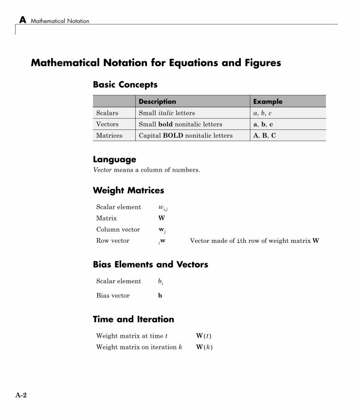
A Mathematical Notation
Mathematical Notation for Equations and Figures
Basic Concepts
Description Example
Scalars Small italic letters a, b, c
Vectors Small bold nonitalic letters a, b, c
Matrices Capital BOLD nonitalic letters A, B, C
LanguageVector means a column of numbers.
Weight Matrices
Scalar element wi,j
Matrix W
Column vector wj
Row vector iw Vector made of ith row of weight matrixW
Bias Elements and Vectors
Scalar element bi
Bias vector b
Time and Iteration
Weight matrix at time t W(t)
Weight matrix on iteration k W(k)
A-2
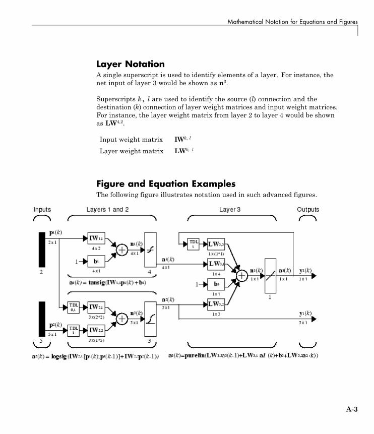
Mathematical Notation for Equations and Figures
Layer NotationA single superscript is used to identify elements of a layer. For instance, thenet input of layer 3 would be shown as n3.
Superscripts k, l are used to identify the source (l) connection and thedestination (k) connection of layer weight matrices and input weight matrices.For instance, the layer weight matrix from layer 2 to layer 4 would be shownas LW4,2.
Input weight matrix IWk, l
Layer weight matrix LWk, l
Figure and Equation ExamplesThe following figure illustrates notation used in such advanced figures.
A-3
A Mathematical Notation
Mathematics and Code EquivalentsThe transition from mathematics to code or vice versa can be made with theaid of a few rules. They are listed here for reference.
Mathematics Notation to MATLAB NotationTo change from mathematics notation to MATLAB notation:
• Change superscripts to cell array indices. For example,
p p1 1→ { }
• Change subscripts to indices within parentheses. For example,
p p2 2→ ( )
and
p p21 1 2→ { }( )
• Change indices within parentheses to a second cell array index. Forexample,
p k p k1 1 1 1( ) { , }− → −
• Change mathematics operators to MATLAB operators and toolboxfunctions. For example,
ab a b→ ∗
Figure NotationThe following equations illustrate the notation used in figures.
n w p w p p bR R= + + + +1 1 1 1 2 2 12, , ,...
A-4
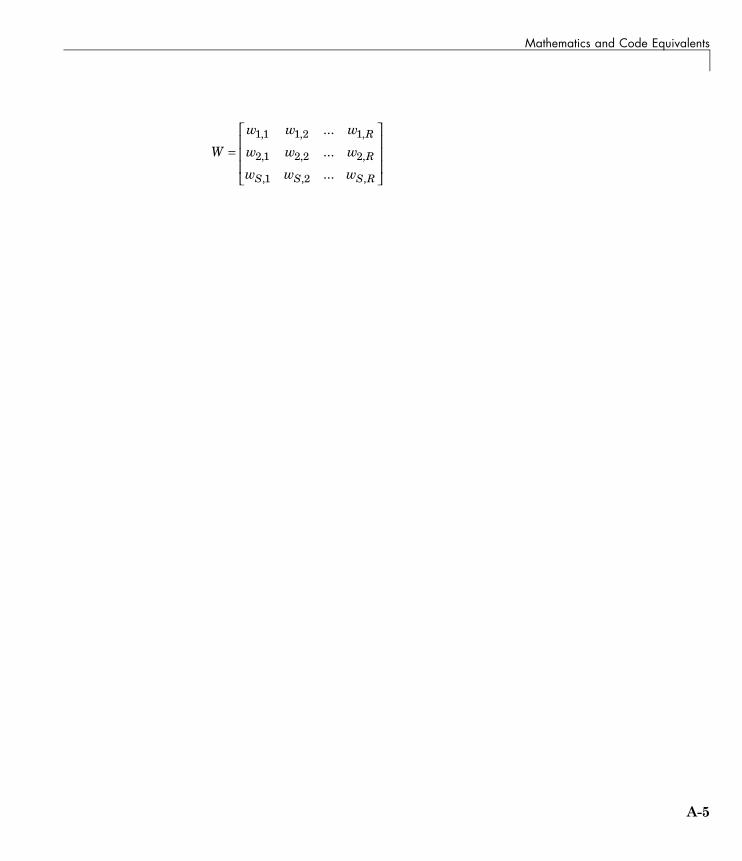
Mathematics and Code Equivalents
W
w w w
w w w
w w w
R
R
S S S R
=⎡
⎣
⎢⎢⎢
⎤
⎦
⎥⎥⎥
1 1 1 2 1
2 1 2 2 2
1 2
, , ,
, , ,
, , ,
...
...
...
A-5

A Mathematical Notation
A-6
B
Blocks for the SimulinkEnvironment
• “Block Library” on page B-2
• “Block Generation” on page B-5
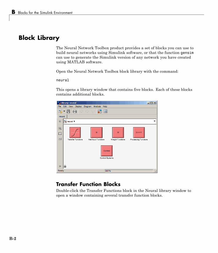
B Blocks for the Simulink Environment
Block LibraryThe Neural Network Toolbox product provides a set of blocks you can use tobuild neural networks using Simulink software, or that the function gensimcan use to generate the Simulink version of any network you have createdusing MATLAB software.
Open the Neural Network Toolbox block library with the command:
neural
This opens a library window that contains five blocks. Each of these blockscontains additional blocks.
Transfer Function BlocksDouble-click the Transfer Functions block in the Neural library window toopen a window containing several transfer function blocks.
B-2
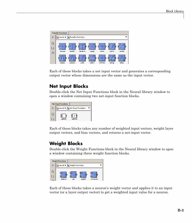
Block Library
Each of these blocks takes a net input vector and generates a correspondingoutput vector whose dimensions are the same as the input vector.
Net Input BlocksDouble-click the Net Input Functions block in the Neural library window toopen a window containing two net-input function blocks.
Each of these blocks takes any number of weighted input vectors, weight layeroutput vectors, and bias vectors, and returns a net-input vector.
Weight BlocksDouble-click the Weight Functions block in the Neural library window to opena window containing three weight function blocks.
Each of these blocks takes a neuron’s weight vector and applies it to an inputvector (or a layer output vector) to get a weighted input value for a neuron.
B-3
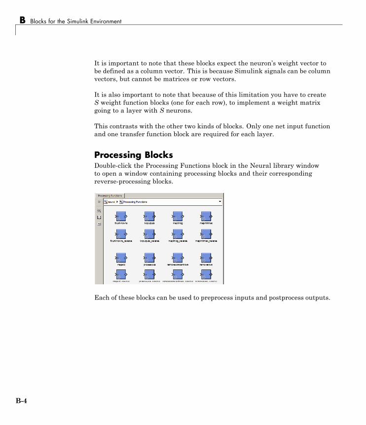
B Blocks for the Simulink Environment
It is important to note that these blocks expect the neuron’s weight vector tobe defined as a column vector. This is because Simulink signals can be columnvectors, but cannot be matrices or row vectors.
It is also important to note that because of this limitation you have to createS weight function blocks (one for each row), to implement a weight matrixgoing to a layer with S neurons.
This contrasts with the other two kinds of blocks. Only one net input functionand one transfer function block are required for each layer.
Processing BlocksDouble-click the Processing Functions block in the Neural library windowto open a window containing processing blocks and their correspondingreverse-processing blocks.
Each of these blocks can be used to preprocess inputs and postprocess outputs.
B-4
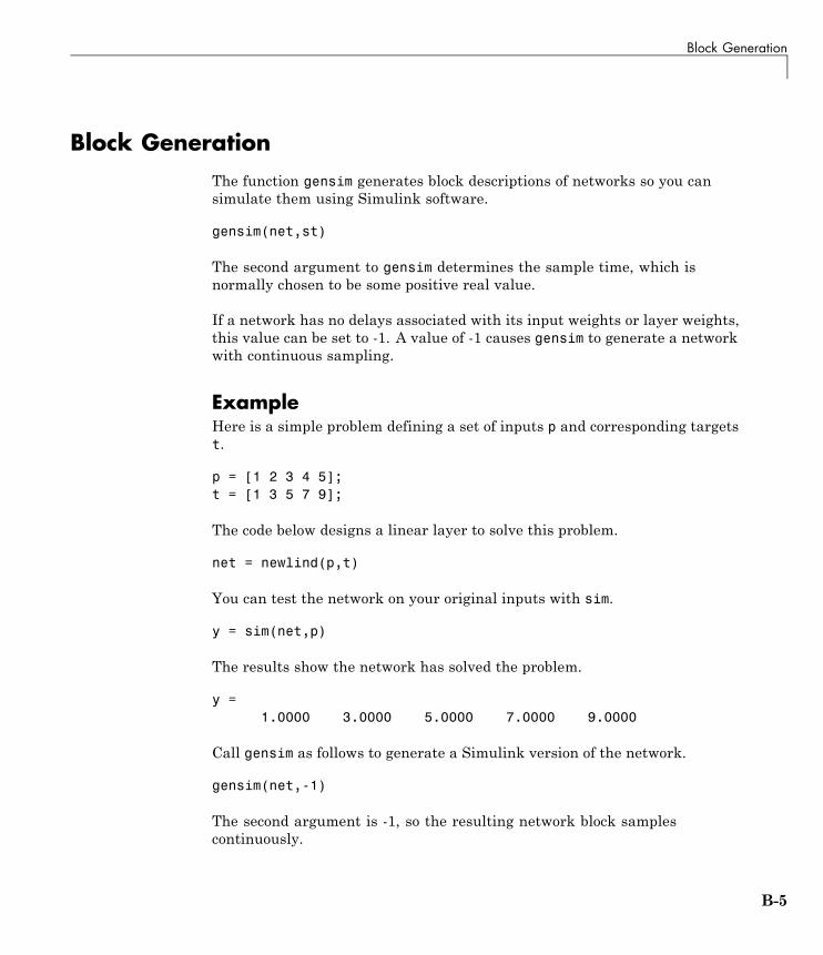
Block Generation
Block GenerationThe function gensim generates block descriptions of networks so you cansimulate them using Simulink software.
gensim(net,st)
The second argument to gensim determines the sample time, which isnormally chosen to be some positive real value.
If a network has no delays associated with its input weights or layer weights,this value can be set to -1. A value of -1 causes gensim to generate a networkwith continuous sampling.
ExampleHere is a simple problem defining a set of inputs p and corresponding targetst.
p = [1 2 3 4 5];t = [1 3 5 7 9];
The code below designs a linear layer to solve this problem.
net = newlind(p,t)
You can test the network on your original inputs with sim.
y = sim(net,p)
The results show the network has solved the problem.
y =1.0000 3.0000 5.0000 7.0000 9.0000
Call gensim as follows to generate a Simulink version of the network.
gensim(net,-1)
The second argument is -1, so the resulting network block samplescontinuously.
B-5
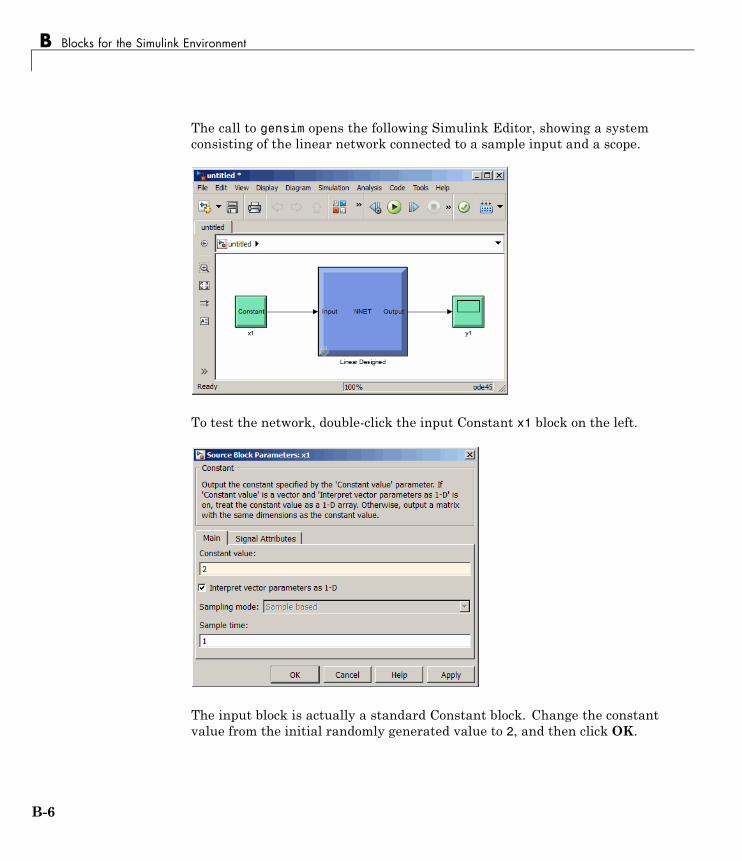
B Blocks for the Simulink Environment
The call to gensim opens the following Simulink Editor, showing a systemconsisting of the linear network connected to a sample input and a scope.
To test the network, double-click the input Constant x1 block on the left.
The input block is actually a standard Constant block. Change the constantvalue from the initial randomly generated value to 2, and then click OK.
B-6
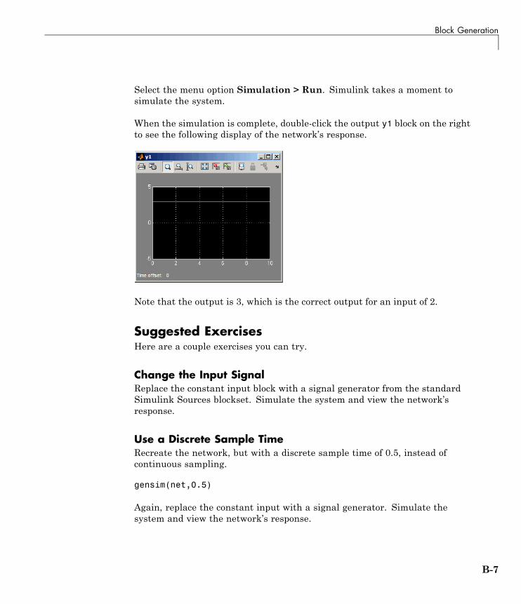
Block Generation
Select the menu option Simulation > Run. Simulink takes a moment tosimulate the system.
When the simulation is complete, double-click the output y1 block on the rightto see the following display of the network’s response.
Note that the output is 3, which is the correct output for an input of 2.
Suggested ExercisesHere are a couple exercises you can try.
Change the Input SignalReplace the constant input block with a signal generator from the standardSimulink Sources blockset. Simulate the system and view the network’sresponse.
Use a Discrete Sample TimeRecreate the network, but with a discrete sample time of 0.5, instead ofcontinuous sampling.
gensim(net,0.5)
Again, replace the constant input with a signal generator. Simulate thesystem and view the network’s response.
B-7

B Blocks for the Simulink Environment
B-8
C
Code Notes
• “Dimensions” on page C-2
• “Variables” on page C-3
• “Functions” on page C-6
• “Code Efficiency” on page C-7
• “Argument Checking” on page C-8
C Code Notes
DimensionsThe following code dimensions are used in describing both the network signalsthat users commonly see, and those used by the utility functions:
Ni = Number of network inputs = net.numInputs
Ri = Number of elements in input i = net.inputs{i}.size
Nl = Number of layers = net.numLayers
Si = Number of neurons in layer i = net.layers{i}.size
Nt = Number of targets
Vi = Number of elements in targeti, equal to Sj, where j is the ithlayer with a target. (A layer n has atarget if net.targets(n) == 1.)
No = Number of network outputs
Ui = Number of elements in outputi, equal to Sj, where j is the ithlayer with an output (A layer n hasan output if net.outputs(n) == 1.)
ID = Number of input delays = net.numInputDelays
LD = Number of layer delays = net.numLayerDelays
TS = Number of time steps
Q = Number of concurrent vectorsor sequences
C-2
Variables
VariablesThe variables a user commonly uses when defining a simulation or trainingsession are
P Network inputs Ni-by-TS cell array, where each elementP{i,ts} is an Ri-by-Q matrix
Pi Initial input delayconditions
Ni-by-ID cell array, where each elementPi{i,k} is an Ri-by-Q matrix
Ai Initial layer delayconditions
Nl-by-LD cell array, where each elementAi{i,k} is an Si-by-Q matrix
T Network targets Nt-by-TS cell array, where each elementP{i,ts} is a Vi-by-Q matrix
These variables are returned by simulation and training calls:
Y Network outputs No-by-TS cell array, where each elementY{i,ts} is a Ui-by-Q matrix
E Network errors Nt-by-TS cell array, where each elementP{i,ts} is a Vi-by-Q matrix
perf Networkperformance
C-3
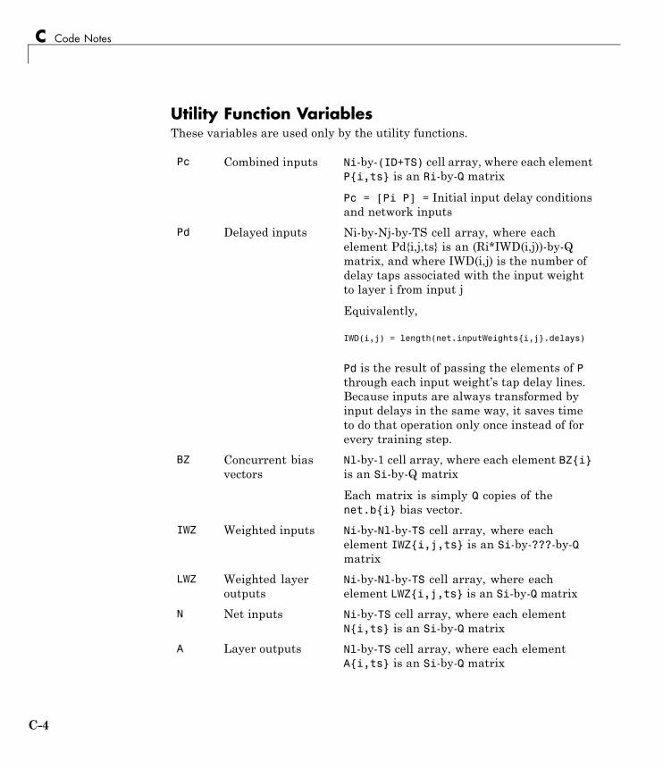
C Code Notes
Utility Function VariablesThese variables are used only by the utility functions.
Pc Combined inputs Ni-by-(ID+TS) cell array, where each elementP{i,ts} is an Ri-by-Q matrix
Pc = [Pi P] = Initial input delay conditionsand network inputs
Pd Delayed inputs Ni-by-Nj-by-TS cell array, where eachelement Pd{i,j,ts} is an (Ri*IWD(i,j))-by-Qmatrix, and where IWD(i,j) is the number ofdelay taps associated with the input weightto layer i from input j
Equivalently,
IWD(i,j) = length(net.inputWeights{i,j}.delays)
Pd is the result of passing the elements of Pthrough each input weight’s tap delay lines.Because inputs are always transformed byinput delays in the same way, it saves timeto do that operation only once instead of forevery training step.
BZ Concurrent biasvectors
Nl-by-1 cell array, where each element BZ{i}is an Si-by-Q matrix
Each matrix is simply Q copies of thenet.b{i} bias vector.
IWZ Weighted inputs Ni-by-Nl-by-TS cell array, where eachelement IWZ{i,j,ts} is an Si-by-???-by-Qmatrix
LWZ Weighted layeroutputs
Ni-by-Nl-by-TS cell array, where eachelement LWZ{i,j,ts} is an Si-by-Q matrix
N Net inputs Ni-by-TS cell array, where each elementN{i,ts} is an Si-by-Q matrix
A Layer outputs Nl-by-TS cell array, where each elementA{i,ts} is an Si-by-Q matrix
C-4
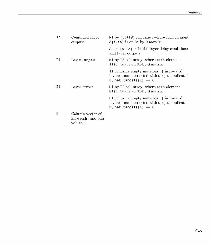
Variables
Ac Combined layeroutputs
Nl-by-(LD+TS) cell array, where each elementA{i,ts} is an Si-by-Q matrix
Ac = [Ai A] = Initial layer delay conditionsand layer outputs.
Tl Layer targets Nl-by-TS cell array, where each elementTl{i,ts} is an Si-by-Q matrix
Tl contains empty matrices [] in rows oflayers i not associated with targets, indicatedby net.targets(i) == 0.
El Layer errors Nl-by-TS cell array, where each elementEl{i,ts} is an Si-by-Q matrix
El contains empty matrices [] in rows oflayers i not associated with targets, indicatedby net.targets(i) == 0.
X Column vector ofall weight and biasvalues
C-5
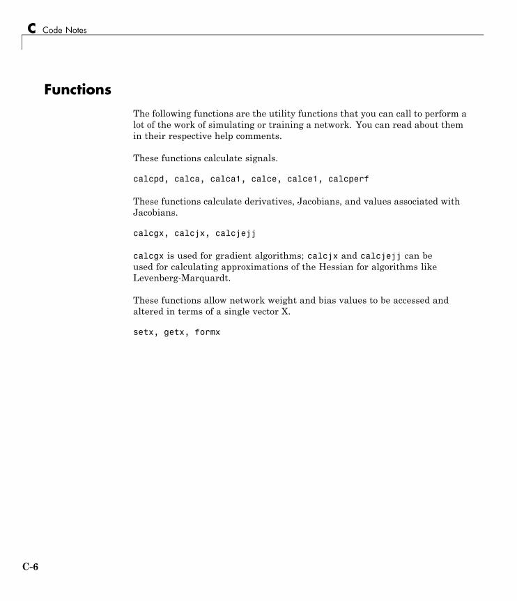
C Code Notes
FunctionsThe following functions are the utility functions that you can call to perform alot of the work of simulating or training a network. You can read about themin their respective help comments.
These functions calculate signals.
calcpd, calca, calca1, calce, calce1, calcperf
These functions calculate derivatives, Jacobians, and values associated withJacobians.
calcgx, calcjx, calcjejj
calcgx is used for gradient algorithms; calcjx and calcjejj can beused for calculating approximations of the Hessian for algorithms likeLevenberg-Marquardt.
These functions allow network weight and bias values to be accessed andaltered in terms of a single vector X.
setx, getx, formx
C-6
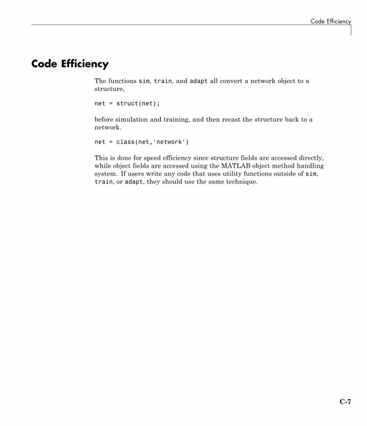
Code Efficiency
Code EfficiencyThe functions sim, train, and adapt all convert a network object to astructure,
net = struct(net);
before simulation and training, and then recast the structure back to anetwork.
net = class(net,'network')
This is done for speed efficiency since structure fields are accessed directly,while object fields are accessed using the MATLAB object method handlingsystem. If users write any code that uses utility functions outside of sim,train, or adapt, they should use the same technique.
C-7

C Code Notes
Argument CheckingThese functions are only recommended for advanced users.
None of the utility functions do any argument checking, which means thatthe only feedback you get from calling them with incorrectly sized argumentsis an error.
The lack of argument checking allows these functions to run as fast aspossible.
For “safer” simulation and training, use sim, train, and adapt.
C-8
Index
IndexAADALINE networks
decision boundary 9-21adapt 1-30adaptFcn
function property 10-9adaptive filters
example 7-11noise cancelation example 7-15prediction example 7-14training 1-30
adaptive linear networks 7-2adaptParam
function property 10-9applications
adaptive filtering 7-10architecture
bias connection 8-48input connection 8-49layer connection 8-49number of inputs 8-48number of layers 8-48number of outputs 8-50number of targets 8-50output connection 8-50target connection 8-50
architecture properties 10-3
Bb
bias vector property 10-13backpropagation
algorithm 2-15batch algorithm 6-11batch training
compared 1-30definition 1-33dynamic networks 1-35static networks 1-33
batch training algorithm 6-31Bayesian framework 8-39benchmark data sets 8-41biasConnect
architecture property 10-4biases
connection 8-48definition 1-4subobject 8-54subobject and network object 10-25subobject property 10-8value 8-56
box distance 6-17
CcachDelayedInputs efficiency property 10-2cell arrays
bias vectors 8-56input P 1-28input vectors 8-58inputs 1-32inputs property 8-50layers property 8-52matrix of concurrent vectors 1-28matrix of sequential vectors 1-31sequence of outputs 1-27sequential inputs 1-26targets 1-32weight matrices 8-56
classificationinput vectors 9-4linear 9-29regions 9-4using probabilistic neural networks 5-10
competitive layers 6-3competitive neural networks
creating 6-4example 6-8
competitive transfer functions 6-3
Index-1
Index
concurrent inputscompared 1-24
configuration settingsdefinition 1-22
configuredefinition 1-21
continuous stirred tank reactor example 4-6control
control design 4-2electromagnet 4-18feedback linearization 4-14feedback linearization (NARMA-L2) 4-3model predictive 4-3model predictive control 4-5model reference 4-3NARMA-L2 4-14plant 4-23plant for predictive control 4-2robot arm 4-24time horizon 4-5training data 4-10
controllerNARMA-L2 controller 4-16
CSTR 4-6custom neural networks 8-46
Ddata
test 2-10training 2-10validation 2-10
dead neurons 6-6decision boundary 9-21
definition 9-4delays
input weight property 10-26layer weight property 10-28
derivFcnfunction property 10-9
dimensionslayer property 10-17
distance 6-10box 6-17Euclidean 6-16link 6-17Manhattan 6-17tuning phase 6-19
distance functions 6-15distanceFcn
layer property 10-18distances
layer property 10-18divideFcn
function property 10-10divideMode
function property 10-10divideParam
function property 10-10dynamic networks
concurrent inputs 1-27sequential inputs 1-25training
batch 1-35incremental 1-32
Eearly stopping
improving generalization 8-35electromagnet example 4-18error weighting 3-40Euclidean distance 6-16examples
continuous stirred tank reactor 4-6demohop1 9-40demohop2 9-40demorb4 5-8electromagnet 4-18nnd10lc 9-31
Index-2
Index
nnd11gn 8-34robot arm 4-24
exporting networks 4-31exporting training data 4-35
Ffeedback linearization 4-2
companion form model 4-14See also NARMA-L2
feedbackDelay output property 10-23feedbackInput output property 10-23feedbackMode output property 10-23feedforward networks 2-5finite impulse response filters
example 9-26flattenTime efficiency property 10-2
Ggeneralization
improving 8-34regularization 8-37
generalized regression networks 5-13gridtop topology 6-11
Hhard limit transfer function
hardlim 9-3hextop topology 6-13hidden layers
definition 1-13home neuron 6-16Hopfield networks
architecture 9-34design equilibrium point 9-36solution trajectories 9-40spurious equilibrium points 9-36stable equilibrium point 9-36target equilibrium points 9-36
horizon 4-5
Iimporting networks 4-31importing training data 4-35incremental training 1-30
static networks 1-30initFcn
bias property 10-25function property 10-10input weight property 10-26layer property 10-18layer weight property 10-28
initParamfunction property 10-11parameter property 10-9
initSettingsinput weight property 10-27layer weight property 10-29
input vectorsclassification 9-4distance 6-10outlier 9-17topology 6-10
input weightsdefinition 1-12subobject 10-26
inputConnectarchitecture property 10-4
inputsconcurrent 1-24connection 8-49input property 10-15number 8-48sequential 1-24subobject 8-50subobject property 10-7
inputWeightssubobject property 10-8
Index-3
Index
IWweight property 10-12
KKohonen learning rule 6-5
Llayer weights
definition 1-12subobject 10-28
layerConnectarchitecture property 10-5
layersconnection 8-49number 8-48subobject 8-52subobject property 10-7
layers property 10-17layerWeights
subobject property 10-8learn
bias property 10-25input weight property 10-27layer weight property 10-29
learnFcnbias property 10-25input weight property 10-27layer weight property 10-29
learning ratesmaximum stable 9-29ordering phase 6-19too large 9-32tuning phase 6-19
learning rulesKohonen 6-5LMS 7-2
See also Widrow-Hoff learning ruleLVQ1 6-41
LVQ2.1 6-45perceptron 9-3Widrow-Hoff 9-27
learning vector quantizationcreation 6-38learning rule 6-45
LVQ1 6-41LVQ network 6-37subclasses 6-37supervised training 6-2target classes 6-37union of two subclasses 6-41
learnParambias property 10-26input weight property 10-27layer weight property 10-29
least mean square error learning rule 7-8linear networks
design 9-23linear transfer functions 9-19linearly dependent vectors 9-32link distance 6-17log-sigmoid transfer function
logsig 2-3log-sigmoid transfer functions 1-5LVQ networks 6-37LW
weight property 10-13
MMADALINE networks 7-4magnet 4-18Manhattan distance 6-17mean square error function 2-15
least 7-8memory reduction 2-18memoryReduction efficiency property 10-3model predictive control 4-5model reference control 4-2
Index-4
Index
Model Reference Control block 4-24
Nname input property 10-15name layer property 10-17name network property 10-2name output property 10-23NARMA-L2 control 4-14NARMA-L2 controller 4-16NARMA-L2 Controller block 4-18neighbor distances plot 6-33neighborhood 6-10net input function
definition 1-4netInputFcn
layer property 10-18netInputParam
layer property 10-19network functions 8-55network layers
competitive 6-3definition 1-8
networksdefinition 8-47dynamic
concurrent inputs 1-27sequential inputs 1-25
static 1-24neural networks
adaptive linear 7-2competitive 6-4custom 8-46feedforward 2-5generalized regression 5-13one-layer 1-10
figure 9-19probabilistic 5-10radial basis 5-2self-organizing 6-2
self-organizing feature map 6-10neurons 1-4
dead (not allocated) 6-5definition 1-4home 6-16See also distance, topologies
NN Predictive Control block 4-6notation
abbreviated 1-7layer 1-13transfer function symbols 1-6
numInputDelaysarchitecture property 10-6
numInputsarchitecture property 10-3
numLayerDelaysarchitecture property 10-6
numLayersarchitecture property 10-3
numOutputsarchitecture property 10-5
numWeightElementsarchitecture property 10-6
Oordering phase learning rate 6-19outlier input vectors 9-17output layers
definition 1-13linear 2-5
outputConnectarchitecture property 10-5
outputsconnection 8-50number 8-50subobject 8-53subobject properties 10-23subobject property 10-7
overdetermined systems 9-32
Index-5
Index
overfitting 8-34
Ppass
definition 9-11perceptron learning rule 9-3
learnp 9-8normalized 9-17
perceptron networklimitations 9-16
perceptron networksintroduction 9-3
performance functionsmodifying 8-37
performFcnfunction property 10-11
performParamfunction property 10-11
plant 4-23plant identification 4-23
NARMA-L2 model 4-14Plant Identification window 4-9plant model 4-2
in model predictive control 4-3plotFcns
function property 10-11plotParams
function property 10-12positions
layer property 10-19posttraining analysis 8-43predictive control 4-5preprocessing 2-7probabilistic neural networks 5-10
design 5-11process parameters
definition 1-22properties that determine algorithms 10-9
Rradial basis
design 5-15efficient network 5-7function 5-2networks 5-2
radial basis transfer function 5-4randtop topology 6-14range
layer property 10-20recurrent networks 9-2regularization 8-37
automated 8-39robot arm example 4-24
Ssample hits plot 6-34self-organizing feature map (SOFM)
networks 6-10batch algorithm 6-11neighbor distances plot 6-33neighborhood 6-10one-dimensional example 6-25sample hits plot 6-34two-dimensional example 6-27weight planes plot 6-35weight positions plot 6-32
self-organizing networks 6-2sequential inputs 1-24simulation 2-28Simulink
generating networks B-5Neural Network Toolbox block library
simulation B-2NNT blockset code C-2
sizebias property 10-26bias vector property 10-26input property 10-17
Index-6
Index
input weight property 10-27layer property 10-20layer weight property 10-29output property 10-25
spread constant 5-6static networks
batch training 1-33concurrent inputs 1-24defined 1-24incremental training 1-30
subobject properties 10-15network definition 8-50
subobject structure properties 10-7subobjects
bias code 8-54bias definition 10-25input 8-50input weight properties 10-26layer 8-52layer weight properties 10-28output code 8-53output definition 10-23target code 8-53weight code 8-54weight definition 10-25
symbolstransfer function representation 1-6
system identification 4-4
Ttan-sigmoid transfer function 2-3tapped delay lines 9-24targets
connection 8-50number 8-50subobject 8-53
time horizon 4-5topologies
self-organizing feature map 6-10
topologies for SOFM neuron locationsgridtop 6-11hextop 6-13randtop 6-14
topologyFcnlayer property 10-21
trainFcnfunction property 10-12
trainingbatch 1-30competitive networks 6-7definition 1-5efficient 2-7incremental 1-30ordering phase 6-22posttraining analysis 8-43self-organizing feature map 6-22styles 1-30tuning phase 6-22
training data 4-10training record 2-23training styles 1-30trainParam
function property 10-12transfer functions
competitive 6-3definition 1-4hard limit in perceptron 9-3linear 9-19log-sigmoid 1-5log-sigmoid in backpropagation 2-3radial basis 5-4tan-sigmoid 2-3
transferFcnlayer property 10-22
transferParamlayer property 10-22
tuning phase learning rate 6-19tuning phase neighborhood distance 6-19
Index-7
Index
Uunderdetermined systems 9-32userdata network property 10-2
Vvectors
linearly dependent 9-32
Wweight and bias value properties 10-12weight function
definition 1-4weight matrix
definition 1-10weight planes plot 6-35
weight positions plot 6-32weightFcn
input weight property 10-28layer weight property 10-30
weightParaminput weight property 10-28layer weight property 10-30
weightsdefinition 1-4subobject code 8-54subobject definition 10-25value 8-56
Widrow-Hoff learning rule 9-27adaptive networks 7-9and mean square error 7-2
Index-8