nested stochastic simulation algorithms for chemical ...eve2/nssa_jcompphys.pdf · nested...

Nested stochastic simulation algorithms for chemicalkinetic systems with multiple time scales

Weinan E a, Di Liu b,*, Eric Vanden-Eijnden c

a Department of Mathematics and PACM, Princeton University, Princeton, NJ 08544, USAb Department of Mathematics, Michigan State University, East Lansing, MI 48824, USA

c Courant Institute of Mathematical Sciences, New York University, New York, NY 10012, USA

Received 24 October 2005; received in revised form 4 April 2006; accepted 7 June 2006

Abstract

We present an e!cient numerical algorithm for simulating chemical kinetic systems with multiple time scales. This algo-rithm is an improvement of the traditional stochastic simulation algorithm (SSA), also known as Gillespie’s algorithm. It isin the form of a nested SSA and uses an outer SSA to simulate the slow reactions with rates computed from realizations ofinner SSAs that simulate the fast reactions. The algorithm itself is quite general and seamless, and it amounts to a smallmodification of the original SSA. Our analysis of such multi-scale chemical kinetic systems allows us to identify the slowvariables in the system, derive e"ective dynamics on the slow time scale, and provide error estimates for the nested SSA.E!ciency of the nested SSA is discussed using these error estimates, and illustrated through several numerical examples.! 2006 Elsevier Inc. All rights reserved.

Keywords: Kinetic Monte-Carlo; Continuous-time Markov chains; Chemical master equations; Stochastic Petri nets; Gillespie algorithm;Averaging theorems; Multiscale numerical methods; Homogenization; Stochastic modeling; Multi-scale computation; Chemical kineticsystems

1. Introduction

The stochastic simulation algorithm (SSA in short), also known as the Gillespie algorithm and originallyintroduced in the context of chemical kinetic systems, has found a wide range of applications in many di"erentfields, including computational biology, chemistry, combustion, and communication networks [20,10,11].Besides being an e"ective numerical algorithm, SSA is also a model for chemical kinetic systems that takes intoaccount the discreteness and finiteness of the molecular numbers as well as stochastic e"ects. This feature makesit an attractive alternative to the approach of using systems of deterministic ODEs, particularly in situationswhen the stochastic e"ects are important [9]. In addition, since SSA uses less modeling assumptions and is there-fore closer to the first principle models, it is often easier to determine the parameters in the model. In fact, themain modeling parameters are the rate functions which can in principle be computed using the rate theories [21].

0021-9991/$ - see front matter ! 2006 Elsevier Inc. All rights reserved.doi:10.1016/j.jcp.2006.06.019

* Corresponding author. Tel.: +1 517 353 8143; fax: +1 517 432 1562.E-mail address: [email protected] (D. Liu).

Journal of Computational Physics xxx (2006) xxx–xxx

www.elsevier.com/locate/jcp

ARTICLE IN PRESS

Please cite this article as: Weinan E et al., Nested stochastic simulation algorithms for chemical ..., Journal of Compu-tational Physics (2006), doi:10.1016/j.jcp.2006.06.019.

mailto:[email protected]

The disadvantage of SSA is that it is computationally more expensive to handle than the systems of ODEs.Besides being stochastic in nature, the system often involves many disparate time scales. This is easy to appre-ciate, since chemical reaction rates often depend exponentially on the activation energy. For a deterministicsystem of ODEs, this results in the sti"ness of the ODEs, for which many e!cient numerical methods havebeen developed [12]. However, the situation for SSA is much less satisfactory.

In recent years, this issue has received a great deal of attention and some important progress has beenmade. The main idea, pursued in di"erent forms by many people, is to model the e"ective dynamics on theslow time scale, by assuming that the fast processes are in quasi-equilibrium [13,25,22,3,4]. In [13], a multi-scale simulation method was proposed in which the slow and fast reactions are simulated di"erently. The slowreactions are simulated using Gillespie algorithm and the fast reactions are simulated using Langevin dynam-ics. In [25], a similar multi-scale scheme is proposed in which the fast dynamics is simulated using deterministicODEs. Both the approaches in [13,25] require that the volume of the system be su!ciently large in addition tohaving well-separated rates. [22] proposes a scheme based on the quasi-equilibrium assumption by assumingthat the probability densities of the fast species conditioned on the slow species is known exactly or can beapproximated, e.g. by normal distributions. The same quasi-equilibrium assumption is used in [3,4], exceptthat the probability density of the fast species conditioned on the slow species is computed via a modified pro-cess called the virtual fast process.

The method proposed in [3,4] is more general than previous methods, but it still has limitations. It assumesthe equilibrium distributions of the fast processes can be approximated by simple functions and the fast speciesare independent of each other at equilibrium. Moreover, the rate functions of the slow processes are alsoassumed to be of special forms and are approximated empirically by solving a system of algebraic equations.These limitations are removed in the recent work, [7], in which a nested SSA is proposed to deal with the timescale issue. This work relies only on the disparity of the rates, and makes no a priori assumption on what theslow and fast variables are, or the analytic form of the rate functions. The recent work in [23] is much closer toour work in spirit. It also adopted a nested structure with inner loop on the fast reactions and the outer loopon the slow reactions. However, the outer loop algorithm is significantly di"erent from ours, without faithfullycapturing the e"ective dynamics on the slow time scale. In particular, they also resort to a partition into slowand fast species, a partition that is avoided in our work.

It is worthwhile to emphasize that, as we will see in Section 3, the algorithm proposed in [7] is quite generaland seamless. In particular, it makes no explicit mentioning of the fast and slow variables. At a first sight, thismight seem surprising, since there are counterexamples showing that algorithms of the same spirit do not workfor deterministic ODEs with separated time scales [8] if the slow variables are not explicitly identified andmade use of. But in the present context, the slow variables are linear functions of the original variables, asa consequence of the fact that the state change vectors {mj}s are constant vectors, and this is the reasonwhy the seamless algorithm works.

However, unlike the original SSA which is exact, the nested SSA is approximate and to understand theerrors in the nested SSA, it is important to understand what the slow and fast variables are and what the e"ec-tive process is on the slow time scale. These issues were dealt with briefly in [7], and one main purpose of thepresent paper is to study them in more detail. This will allow us to estimate the optimal numerical parametersand the overall cost of the algorithm. In addition, we will discuss various extensions of the nested SSA, as wellas important implementation issues such as adaptively determining slow and fast processes.

The paper is organized as follows. In Section 2, we define the slow variables and derive the e"ective dynam-ics on the slow time scale for chemical kinetic systems with two disparate time scales. Section 3 introduces thenested SSA for the special case when the system has two disparate time scales. Error estimates for the nestedSSA are proved and illustrated through numerical examples. We also elaborate on why the nested SSA algo-rithm is seamless, and when a similar seamless algorithm can be developed in the context of ordinary di"er-ential equation such as, for instance, the ones that arises from the chemical kinetic system in the large volumelimit. Then in Section 4, we show how to adaptively determine the partition of the system into slow and fastreactions during the simulation. Finally, in Section 5, we discuss the e"ective dynamics and nested SSA forsystem with multiple (more than two) well-separated time scales. In this case, both the averaging principleand the nested SSA can be applied iteratively, similar to the case in iterated homogenization [1]. We also studythe system over the di"usive time scale.

2 W. E et al. / Journal of Computational Physics xxx (2006) xxx–xxx

ARTICLE IN PRESS


2. Chemical kinetic systems with two disparate time scales

We will discuss first the case when the chemical kinetic system has two well-separated time scales. Systemswith multiple (more than two) disparate time scales will be discussed in later sections.

2.1. The general setting

Let us first fix some notations. We will consider the time evolution of an isothermal, spatially homogeneousmixture of chemically reacting molecules contained in a fixed volume V. Suppose there are NS species of mol-ecules Si!1;...;NS involved, with MR reactions Rj!1;...;MR . Let xi be the number of molecules of species Si. Then thestate-space of the system is given by

X " NNS #1$and we will denote the elements in this state-space by x ! #x1; . . . ; xNS $ 2 X. Each reaction Rj can be charac-terized by a rate function aj(x) and a state change (or stoichiometric) vector mj which satisfies x% mj 2 X for allx 2 X such that aj(x) 6! 0. We write

Rj ! #aj; mj$; R ! fR1; . . . ;RMRg: #2$Given state x, the occurrences of the reactions on an infinitesimal time interval dt are independent of eachother and the probability for reaction Rj to happen during this time interval is given by aj(x)dt. The stateof the system after reaction Rj is x + mj. We assume that the state space is finite, as is the case for all chemicalreactions in real life. The rate functions usually take the form of polynomials of x.

Consider the observable u#x; t$ ! Exf #X t$, where Xt is the state variable at time t, and Ex denotes expecta-tion conditional on Xt=0 = x. u(x, t) satisfies the following backward Kolmogorov equation:

ou#x; t$ot

!X

j

aj#x$#u#x% mj; t$ & u#x; t$$ !: #Lu$#x; t$: #3$

The operator L is the infinitesimal generator of the Markov process associated with the chemical kineticsystem.

Now we turn to chemical kinetic systems with two disparate time scales. Assume that the rate function of achemical kinetic system R = {(a,m)} has the following form:

a#x$ ! #as#x$; !&1af#x$$; #4$where !' 1 represents the ratio of time scales of the system. The corresponding reactions and the associatedstate change vectors can be grouped accordingly:

Rs ! f#as; ms$g; Rf ! 1

!af ; mf

! "# $: #5$

We call Rs the slow reactions and Rf the fast reactions.To illustrate these definitions, consider the following simple example system that we will investigate in more

detail later:

S1 ¢a1

a2S2; S2 ¢

a3

a4S3; S3 ¢

a5

a6S4: #6$

The reaction rates and the state change vectors are

a1 ! 105x1; m1 ! #&1;%1; 0; 0$;a2 ! 105x2; m2 ! #%1;&1; 0; 0$;a3 ! x2; m3 ! #0;&1;%1; 0$;a4 ! x3; m4 ! #0;%1;&1; 0$;a5 ! 105x3; m5 ! #0; 0;&1;%1$;a6 ! 105x4; m6 ! #0; 0;%1;&1$:

#7$

W. E et al. / Journal of Computational Physics xxx (2006) xxx–xxx 3

ARTICLE IN PRESS


For this system, there are four species of molecules (NS = 4) and six reactions channels (MR = 6). From thereaction rates, it can be seen that the first and the third isomerization reactions are faster than the second isom-erization reaction. We can partition the reactions into fast and slow groups:

Rs ! f#a3; m3$; #a4; m4$g; Rf ! f#a1; m1$; #a2; m2$; #a5; m5$; #a6; m6$g: #8$

If the initial values of the xis are of O(1), the ratio of the time scales is of the order ! = 10&5. Notice that everyvariable xi, i = 1, 2, 3, 4, is involved in at least one fast reaction so there is no slow species. On the other hand,the variables y1 = x1 + x2 and y2 = x3 + x4 are conserved during the fast reactions. In other words, each xi,i = 1, 2, 3, 4, evolves over the fast time scale of O(!) whereas yi, i = 1, 2 evolves over the slow time scale ofO(1). Fig. 1 gives the time evolution of y1 = x1 + x2 and x3 on an intermediate time scale of O(10&3) startingfrom the initial value (x1,x2,x3,x4) = (13,3,3,3). It can been seen that x3 changes its value many times while y1keeps unchanged on this intermediate time scale.

2.2. E!ective dynamics on the slow time scale

For the kind of systems discussed above, very often we are interested mostly in the e"ective dynamics overthe slow time scale. In this section we will derive the model for this e"ective dynamics.

The analysis is built upon the perturbation theory developed in [17,19,14–16]. First we need to understandwhat the slow variables are in the system. Let v be a function of the state variable x, which we call an obser-vable. We say v(x) is a slow observable if it does not change during the fast reactions, i.e. if for any x and anystate change vector mfj associated with the fast reactions one has

v x% mfj% &

! v#x$: #9$

This is equivalent to saying that the slow observables are conserved quantities for the fast process Rf defined in(5). A general representation of such observables is given by special slow observables which are linear func-tions satisfying (9). We call such slow observables slow variables. It is easy to see that v(x) = b Æ x is a slowvariable if

b ( mfj ! 0; #10$

for all fmfjgs. The set of such vectors form a linear subspace in RNS . Let b1, b2, . . . ,bJ be a set of basis vectors ofthis subspace, and let

yj ! bj ( x for j ! 1; . . . ; J ; #11$

0 0.5 1 1.5

x 10–3

0

2

4

6

8

10

12

14

16

18

Time

Mol

ecul

es

x1+x

2

x3

Fig. 1. Evolution of slow variable y1 = x1 + x2 and fast variable x3 on the intermediate timescale.


ARTICLE IN PRESS


then y1, y2, . . . ,yJ defines a complete set of slow variables, i.e. all slow observables can be expressed as func-tions of y1, y2, . . . ,yJ. We define the slow variable y as

y ! #y1; ( ( ( ; yJ $ #12$

and we will denote by Y the space over which y is defined. The state exchange vectors associated with the slowvariables are naturally defined as:

!msi ! #b1 ( msi ; . . . ; bJ ( msi $; i ! 1; . . . ;Ns: #13$

We will also adopt the notion of virtual fast process, defined in [3]. This is an auxiliary process that containsthe fast reactions only, assuming, as we do now, that the set of fast and slow reactions do not change overtime. This turns out to be a quite restrictive assumption and in later sections we will discuss the modificationsneeded when this assumption is no longer satisfied. Now we derive the e"ective dynamics on the slow timescale using singular perturbation theory. We assume that, for each fixed value of the slow variable y, the vir-tual fast process admits a unique equilibrium distribution ly(x) in the state space. We define a projection oper-ator P by

#Pv$#y$ !X

x2Xly#x$v#x$: #14$

By this definition, for any v : X ! R, Pv depends only on the slow variable y, i.e. Pv : Y ! R.The backward Kolmogorov equation for the multi-scale chemical kinetic system with reaction channels as

in (5) reads:

ouot

! L0u%1

!L1u: #15$

where L0 and L1/! are the infinitesimal generators associated with the slow and fast reactions, respectively: forany f : X ! R,

#L0f $#x$ !XM s

j!1

asj#x$#f #x% msj$ & f #x$$;

#L1f $#x$ !XM f

j!1

afj#x$#f #x% mfj$ & f #x$$;#16$

where Ms is the number of slow reactions in Rs and Mf is the number of fast reactions in Rf. Look for a solu-tion of (15) in the form of

u ! u0 % !u1 % !2u2 % ( ( ( #17$

Inserting this into (15) and equating the coe!cients, we arrive at the hierarchy of equations:

L1u0 ! 0;

L1u1 ! ou0ot & L0u0;

L1u2 ! ( ( (

8><

>:#18$

The first equation implies that u0 belongs to the null-space of L1, which by the ergodicity assumption of thefast process, is equivalent to

u0#x; t$ ! U#b ( x; t$ ) U#y; t$; #19$for some U yet to be determined. Inserting (19) into the second equation in (18), gives (using the explicitexpression for L0)

L1u1#x; t$ !oU#b ( x; t$

ot&XM s

i!1

asi #x$#U#b ( #x% msi $; t$ & U#b ( x; t$$

! oU#y; t$ot

&XM s

i!1

asi #x$#U#y % !msi ; t$ & U#y; t$$: #20$


ARTICLE IN PRESS


This equation requires a solvability condition, namely that the right-hand side be perpendicular to the leftnull-space of L1. By the ergodicity assumption of the fast process, this amounts to requiring that

oUot

!XM s

i!1

!asi #y$#U#y % !msi$ & U#y$$; #21$

where

!asi #y$ ! #Pasi $#y$ !X

x

asi #x$ly#x$: #22$

(21) is the e"ective dynamics on the slow time scale, and the e"ective reaction kinetics on this time scale aregiven in terms of the slow variable by

R ! #!as#y$;!ms$: #23$

The accuracy of the approximation of u by u0 can be estimated as follows. From (18) and (21), it follows that

oot

& L0 &1

!L1

! "#u& u0 & !u1$ ! L0 %

1

!L1 &

oot

! "#u0 % !u1$ ! ! L0 &

oot

! "u1; #24$

where u1 is to be obtained by solving (20). Assuming that u(x, 0) = u0(x, 0) = f(b Æ x), the above equality meansthat on fixed time-intervals

u& u0 ! O#!$: #25$

2.3. Seamless form of the limiting theorem

The limiting dynamics in (21) can be reformulated on the original state space X. Indeed, it is easy to checkthat (21) is equivalent to

ou0ot

!XM s

i!1

!asi#b ( x$#u0#x% msi $ & u0#x$$; #26$

in the sense that if u0(x, t = 0) = f(b Æ x), then

u0#x; t$ ! U#b ( x; t$; #27$

where U#y; t$ solves (21) with the initial condition U#y; 0$ ! f #y$. The fact that (21) can be reformulated as(26) is the key reason why the nested SSA presented in Section 3 is a seamless algorithm that does not requireto explicitly determine what the slow variables y = b Æ x are.

2.4. The example revisited

We now go back to the example (6) to illustrate these constructions. The fast reactions Rf ! f#1! af ; mf$g have

the following form:

af1 ! 105x1; mf1 ! #&1;%1; 0; 0$;af2 ! 105x2; mf2 ! #%1;&1; 0; 0$;af5 ! 105x3; mf5 ! #0; 0;&1;%1$;af6 ! 105x4; mf6 ! #0; 0;%1;&1$:

#28$

The slow reactions Rs = {(as,ms)} are

as3 ! x2; ms3 ! #0;&1;%1; 0$;as4 ! x3; ms4 ! #0;%1;&1; 0$:

#29$


ARTICLE IN PRESS


The slow variables are

y1 ! x1 % x2; y2 ! x3 % x4: #30$

Notice that for each fixed set of values (y1,y2), the virtual fast process has a unique equilibrium distribution lygiven by:

ly1;y2#x1; x2; x3; x4$ !

y1!y2!x1!x2!x3!x4!

#1=2$y1#1=2$y2dx1%x2!y1dx3%x4!y2 : #31$

The e"ective dynamics on the slow time scale is given by the slow reactions with rate functions averaged withrespect to these distributions

!as3 ! Px2 !x1 % x2

2! y1

2; !ms3 ! #&1;%1$;

!as4 ! Px3 !x3 % x4

2! y2

2; !ms4 ! #%1;&1$:

#32$

3. The nested stochastic simulation algorithm

In this section, we introduce a nested stochastic simulation algorithm for chemical kinetic systems with twodisparate rates. We discuss the convergence and e!ciency of the scheme and illustrate them through an exam-ple of a virus infection model.

3.1. The stochastic simulation algorithm (SSA)

First, let us review briefly the standard stochastic simulation algorithm for chemical kinetic systems, pro-posed in [10,11] (see also [2]), also known as the Gillespie algorithm. Suppose we are given a chemical kineticsystem with reaction channels Rj = (aj,mj), j = 1, 2, . . ., MR. Let

a#x$ !XMR

j!1

aj#x$: #33$

Assume that the current time is tn, and the system is at state Xn. We perform the following steps:

(1) Generate independent random numbers r1 and r2 with uniform distribution on the unit interval (0,1]. Let

dtn%1 ! & ln r1a#Xn$

; #34$

and kn+1 be the natural number such that

1

a#Xn$Xkn%1&1

j!0

aj#Xn$ < r2 61

a#Xn$Xkn%1

j!0

aj#Xn$; #35$

where a(0) = 0 by convention.(2) Update the time and the state of the system by

tn%1 ! tn % dtn%1; Xn%1 ! Xn % mkn%1: #36$

Then repeat.

3.2. Nested SSA for system with two separated time scales

In [7], a modified SSA with a nested structure is proposed to simulate the chemical kinetic systems withmultiple time scales. The process at each level of the time scale is simulated with an SSA with some possiblymodified rates. Results from simulations on fast time scales are used to compute the rates for the SSA atslower time scale. For simple systems with only two time scales, the nested SSA consists of two SSAs


ARTICLE IN PRESS


organized with one nested in the other: An outer SSA for the slow reactions only, but with modified slow rateswhich are computed in an inner SSA modeling fast reactions only. Let tn, Xn be the current time and state ofthe system, respectively. The nested SSA for systems with two time scales does the following:

(1) Inner SSA: Run N independent replicas of SSA with the fast reactions Rf = {(!&1 af,mf})} only, for a timeinterval of T0 + Tf. During this calculation, compute the modified slow rates for j = 1,. . .,Ms

~asj !1

N

XN

k!1

1

T f

Z T f%T 0

T 0

asj#Xks$ds; #37$

where X ks is the result of the kth replica of this auxiliary virtual fast process at virtual time s whose initial

value is X kt!0 ! Xn, and T0 is a parameter we choose in order to minimize the e"ect of the transients to

the equilibrium in the virtual fast process.(2) Outer SSA: Run one step of SSA for the modified slow reactions ~Rs ! #~as; ms$ to generate (tn+1,Xn+1)

from (tn,Xn).Then repeat.

Let us note that the algorithm as presented is completely seamless and general. We do not need to knowwhat the slow and fast variables are and certainly we do not need to make empirical approximations to getthe e"ective slow rates. The reason why the algorithm works stems from (26), which shows that the e"ectiveequation for the slow variables living in Y can in fact be reformulated on the original state space X. However,it is worth noting that this conclusion is specific to SSA and, it would in general not be true for systemsdescribed by (ordinary or stochastic) di"erential equation rather than a Markov chain. We elaborate on thispoint in Section 3.6.

Without fully realizing the e"ective dynamics (21), in the nested SSA proposed in [23], the outer SSA isadvanced by picking up the next slow reaction using rates without being averaged with respect to the fast reac-tions, which will definitely induce a significant error in the scheme.

In the HMM (heterogeneous multi-scale method) [5] language, the macro-scale solver is the outer SSA, thedata that need to be estimated is the e"ective rates for the slow reactions. These data are obtained by simu-lating the virtual fast process which plays the role of micro-scale solvers here.

3.3. Convergence of the nested SSA

The original SSA is an exact realization of the chemical kinetic system. The nested SSA, on the other hand,is an approximation. The errors in the nested SSA can be analyzed using the same strategy as in [6].

To begin with, since the state space is finite, it is easy to show that the virtual fast process is u-irreducibleand satisfies the stability condition in [18]. Hence for any test function g : X ! R, there exist positive con-stants R and a such that

supx2X

#eL1tg$#x$ & #Pg$#b ( x$'' '' 6 Re&at: #38$

Denote by ~X t the solution of the nested SSA. Consider the observable v#x; t$ ! Exf #b ( ~X t$ where the expecta-tion for f is with respect to the randomness in the outer SSA only. v(x, t) satisfies a backward Kolmogorovequation similar to (26), in which the averaged rate !asj in (22) are replaced by the random rates ~asj obtainedfrom (37) in the current realization of the inner SSA:

ov#x; t$ot

! ~Lv#x; t$; #39$

where

~Lv#x; t$ !XM s

j!1

~asj#b ( x$#v#x% msj$ & v#x$$: #40$

Let u(x, t) be the solution of the system (15) with u(x, 0) = f(b Æ x). We have the following theorem:


ARTICLE IN PRESS


Theorem 3.1. For any T > 0, there exist constants C and a independent of (N,T0,Tf) such that,

sup06t6T ;x2X

Ejv#x; t$ & u#x; t$j 6 C !% e&aT 0=!

1% T f=!% 1(((((((((((((((((((((((((

N#1% T f=!$p

!

: #41$

Proof. Let X kt be the kth realization at the virtual time t in the inner SSA. We have

Ej~as#x$ & !as#x$j2 ! 1

N 2 Ex1

T f

X

k

Z T 0%T f

T 0

#as#Xkt $ & !as#x$$dt

'''''

'''''

2

! 1

T 2fN

2

X

k

Ex

Z T 0%T f

T 0


''''

''''2

% 1

T 2fN

2

X

k 6!l

Ex

Z T 0%T f

T 0

#as#Xkt $

& !as#x$$dtZ T 0%T f

T 0

#as#X lt0$ & !as#x$$dt0

!: A1 % A2: #42$

where Ex denotes expectation conditional on Xkt!0 ! x. Using (38), we get the following estimate

A1 !2

T 2fN

2

X

k

Ex

Z T 0%T f

T 0

#as#X kt $ & !as#x$$ * EXk

t

Z T 0%T f

t#as#X k

s$ & !as#x$$dsdt! "

6 2

T 2fN

2

X

k

Ex

Z T 0%T f

T 0

jas#X kt $ & !as#x$j

Z T 0%T f

tRjasje&a#s&t$=! dsdt

6 4Rjasj2 e&aT f=! & 1% aT f=!) *

N#aT f=!$26 C

N#1% T f=!$: #43$

At the same time, we have from (38)

A2 61

T 2fN

2

X

k 6!l

Ex

Z T 0%T f

T 0


Z T 0%T f

T 0

#as#X lt0$ & !as#x$$dt0

''''

''''

6 1

T 2f

E

Z T 0%T f

T 0

#as#X kt $ & !as#x$$dt

''''

''''2

6 R2jasj2e&2aT 0=!#1& e&aT f=!$2

#aT f=!$26 Ce&2aT 0=!

#1% T f=!$2: #44$

Hence we have

Ej~as#x$ & !as#x$j2 6 Ce&2aT 0=!

#1% T f=!$2% 1

N#1% T f=!$

!

; #45$

which implies that

Ek~L& PL0Pk 6 C0 e&aT 0=!

1% T f=!% 1(((((((((((((((((((((((((

N#1% T f=!$p

!

: #46$

The finiteness of the state space implies the boundedness of v. Let w(x, t) be the solution of the effective Eq.(21) with w(x, 0) = f(x). We have

dEjv& wjdt

! Ej#~L& PL0P $v% PL0P#v& w$j 6 CEjv& wj% Ce&aT 0=!

1% T f=!% 1(((((((((((((((((((((((((

N#1% T f=!$p

!

; #47$

which, together with (25), gives (41). h


ARTICLE IN PRESS


3.4. E"ciency of the nested SSA

Now we discuss the e!ciency of the nested SSA based on the error estimate (41). Given a chemical kineticsystem with R = {(aj,mj)}, we assume that the total rate a#x$ !

Paj#x$ does not fluctuate a lot in time. Given

an error tolerance k, we choose the parameters in the nested SSA such that each term in (41) is less than O(k).One possible choice of the parameters is

T 0 ! 0; N ! 1% !&1T f !1

k: #48$

The total cost for the nested SSA over a time interval of O(1) is

cost ! O#N#1% T 0=!% T f=!$$ ! O1

k2

! ": #nested SSA$ #49$

The cost of the direct SSA is

cost ! O1

!

! "; #direct SSA$ #50$

since the time step size is of order !. When ! ' k2, the nested SSA is much more e!cient than the directSSA.

Next we discuss the influence of the other numerical parameters on the e!ciency. The parameter T0 whichplays the role of numerical relaxation time does not influence much the e!ciency. Given the same error tol-erance k, for the last term in the error estimate (41) to be less than O(k), we need to have

N#1% !&1T f$ P O1

k2

! ": #51$

This implies that the cost satisfies

cost P O#N#1% !&1T f$$ ! O1

k2

! "; #nested SSA$ #52$

!which is the same as (50) regardless the value of T0. The above argument also implies that the cost of O(1/k2)is optimal for the nested SSA to achieve an error tolerance of k.

We then move to the e"ect of parameter N, the number of realizations for inner SSA. Suppose we takeN = 1, i.e. only one realization of the fast process in the inner SSA. For the error estimate (41) to satisfythe same error tolerance k, we have to choose

1% !&1T f !1

k2: #53$

The cost of the nested SSA is given by

cost ! O#N#1% !&1T f$$ ! O1

k2

! "; #nested SSA$ #54$

which is the minimum cost of SSA for error tolerance k as discussed above. This implies that using multi-ple realizations in the inner SSA does not increase the e!ciency of the overall scheme either. But usingmultiple realizations allows us to speed up the computation on parallel computers. Suppose we use Mprocessors to simulate independent copies of the fast processes, then the computing time on each proces-sor reduces to

cost ! O1

Mk2

! "; #nested SSA per processor$ #55$

for simulating the inner SSA. Another technique for speeding up the computation of the nested scheme is toestablish an on-the-fly chart for ~as#y$ and re-use the same data of ~as#y$ whenever the slow process revisit thesame slow state y. This is especially e"ective when the state space is small.


ARTICLE IN PRESS


3.5. A numerical example: A virus infection model

A virus infection model was proposed in [24] as an example of the failure of modeling genetic reacting net-works with deterministic dynamics. The model is studied in [13] as an example of reactions with disparaterates. The reactions considered in this model (MR = 6) are listed in Table 1. The reacting species that needto be modeled are genome, struct, template and virus (Ns = 4). Genome is the vehicle of the viral genetic infor-mation which can take the form of DNA, positive-strand RNA, negative-strand RNA, or some other variants.Struct represents the structural proteins making up the virus. Template refers to the form of the nucleic acidthat is transcribed and involved in catalytically synthesizing every viral component. The nucleotides andamino acids are assumed to be available at constant concentrations.

When template > 0, the production and degradation of struct, which are the third and fifth reactionsmarked with * in Table 1, are faster than the others. From the reaction rates, we can see that the ratio of timescales is about ! = 10&3. In the system that consists of only the fast reactions, struct has an equilibrium mea-sure of a Poisson distribution with the parameter k = 500 · template such that

Ptemplate#struct ! n$ ! #500* template$n

n!exp#&500* template$: #56$

Notice that struct only shows up in the last slow reaction. The reduced dynamics in the form of the slow reac-tions (a1,2,4,6) with the rates averaged with respect to the quasi-equilibrium of the fast reactions (a3,5) can begiven as a system with four reactions given in Table 2.

To test the convergence and e!ciency of the nested SSA and compare it with the direct SSA, we use themean value and the variance of template at time T = 20 as a benchmark. The initial condition is chosen to be:

#struct; genome; template; virus$ ! #0; 0; 10; 0$: #57$

A computation of this average by a direct SSA using N0 = 106 realizations led to

template ! 3:7170+ 0:005; var#template$ ! 4:9777+ 0:005: #58$

This calculation took 34806.39 s of CPU time on our machine. For the nested SSA, we make a series of sim-ulations in which we choose the size of the ensemble and the simulation time of the inner SSA according to

#N ; T 0; T =!$ ! #1; 0; 22k$; #59$

for di"erent values of k = 0, 1, 2, 3, . . .. The error estimate in (41) then implies that the error d should decaywith rate:

d ! O#2&k$: #60$

Table 3 gives the total CPU time and the obtained values of template and var(template) with the parameters ofinner SSA chosen according to (59) and using N0 = 106 realizations of the outer SSA (same as in the directSSA). The relative errors on template is shown in Fig. 2.

Table 1Reaction channels of the virus infection model

Nucleotides !a1!1:*templategenome

Nucleotides % genome !a2!:025*genometemplate

Nucleotides % aminoacids !a3!1000*templatestruct,

Template !a4!:25*templatedegraded

Struct !a5!1:9985*structdegraded=secreted,

Genome % struct !a6!7:5d&6&genome*structvirus


ARTICLE IN PRESS


3.6. Some remarks on the large volume limit

As explained in Section 2.3, because the limiting equation on the slow time scale can be written as (26)on the original state space X, the nested SSA presented in Section 2.3 always works in the context ofchemical kinetic systems. This is somewhat surprising since similar statements do not hold in the caseof ordinary or stochastic di"erential equations with multiple time scales. Here we make some remarks con-cerning this.

Consider the ordinary di"erential equation

_X t !1

ef #X t$ % g#X t$; #61$

for some variable X t 2 Rn. Assume that there exists a vector valued function u : Rn ! Rm#m < n$ such that:

(1) We have

f #x$ (ru#x$ ! 0; #62$

(2) For each fixed y 2 Rm, the dynamics

_X ft ! f #X f

t $; #63$

is ergodic on the level set u(x) = y with respect to the equilibrium distribution dly(x) (which might not beatomic).

Then Yt = u(Xt) are slow variables satisfying the following equation:

_Y t ! H#Y t$; #64$

where

H#y$ !Z

Rng#x$ (ru#x$dly#x$: #65$

(64) holds provided that conditions (1) and (2) are satisfied and the expectation in (65) is finite. The existenceof a limiting dynamics has been exploited in [26] to construct e!cient algorithms for the simulation of (61)when ! ' 1. However, these algorithms cannot, in general, be put in a seamless form because the mappingu defining the slow variable is usually nonlinear, in contrast to what happens in the context of chemical kineticsystems. In particular, it is easy to see that the equation

Table 2The reduced virus infection model

Nucleotides !a1!1:*templategenome

Nucleotides % genome !a2!:025*genometemplate

Template !a4!:25*templatedegraded

Genome % struct !a6!3:75d&3*genome2*structvirus

Table 3E!ciency of the nested SSA for the virus infection model

Tf/! 1 4 16 64

CPU 154.8 461.3 2068.2 9190.9template 4.027 3.947 3.796 3.757var (template) 5.401 5.254 5.007 4.882


ARTICLE IN PRESS


_X t ! G#u#X t$$; #66$

where

G#y$ !Z

Rng#x$dly#x$; #67$

will in general not be equivalent to (64) (in the sense that u#X t$ 6! Y t), unless $u(x) is a function of y only, i.e.

ru#x$ ! J#u#x$$; #68$

for some J : Rm ! Rn * Rm. Only if (68) is satisfied do we have H(y) = G(y)J(y) and u#X t$ ! Y t.Condition (68) is rather restrictive. Quite remarkably, however, it is satisfied for the system of ordinary dif-

ferential equations that arise from (15) in the large volume limit. Indeed, assuming that the number of mol-ecules of each species is large, and after appropriate rescaling of the variables, it is well known that (15) leadsto

_X t !1

!

XM f

j!1

afj#X t$mfj %XM s

j!1

asj#X t$msj: #69$

These equations are in the form of (61), and it is easy to see that if (b1, . . . ,bm) is a basis of vector satisfyingbi ( mfj, then

uj#x$ ! bj ( x; #70$

satisfy (62) and (68) (with J being the constant matrix with rows consisting of the vector bj). This suggests that,in the limit as !! 0, the solution of (69) converges to the solution of

_X t !XM s

j!1

!asj#b ( X t$msj: #71$

Here

!asj#y$ !Z

Rnasj#x$dly#x$; #72$

where dly(x) is the equilibrium of the fast process

_X ft !

1

!

XM f

j!1

afj#Xft $m

fj: #73$

1 2 3 4102

101

k

Err

or

-

-

Fig. 2. Relative errors of template using the nested SSA for the virus infection model.


ARTICLE IN PRESS


Since (72) can be approximated by

~as !1

T f

Z T f

0

asj#Xft $dt; #74$

for some appropriate Tf, this naturally leads to a very simple and seamless nested algorithm for simulating (69)for small !: The inner loop solves the virtual fast system (63) for some time Tf; the outer loop solves (71), with!asJ approximated by !asj#y$ ! asj#X f

T f$.

For instance, in the large volume limit, the ODEs corresponding to the simple example treated in Section2.4 are

_X 1 ! 105#&X 1 % X 2$;_X 2 ! 105#X 1 & X 2$ & X 2 % X 3;_X 3 ! 105#&X 3 % X 4$ & X 3 % X 2;_X 4 ! 105#X 3 & X 4$:

8>>><

>>>:#75$

In this case, the slow variables are Y1 = X1 + X2 and Y2 = X3 + X4, and it is easy to see that the fast processdrives the variables toward the fixed point

X f1 ! X f

2 ! Y 1=2; X f3 ! X f

4 ! Y 2=2; #76$

meaning that dly(x) is atomic in this case

dly#x$ ! d#x1 & y1=2$d#x2 & y1=2$d#x3 & y2=2$d#x4 & y2=2$dx1 dx2 dx3 dx4: #77$

Hence from (64), the limiting dynamics is

_Y 1 ! &X 2 % X 3 ! #&Y 1 % Y 2$=2;_Y 2 ! &X 3 % X 2 ! #Y 1 & Y 2$=2;

(

#78$

which from (71), can also be written in terms of the original variables as

_X 1 ! 0;_X 2 ! #&X 2 % X 3$;_X 3 ! #&X 2 % X 3$;_X 4 ! 0:

8>>><

>>>:#79$

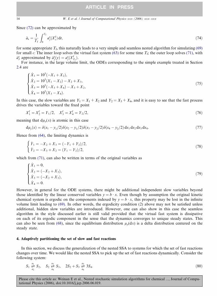
However, in general for the ODE systems, there might be additional independent slow variables beyondthose identified by the linear conserved variables y = b Æ x. Even though by assumption the original kineticchemical system is ergodic on the components indexed by y = b Æ x, this property may be lost in the infinitevolume limit leading to (69). In other words, the ergodicity condition (2) above may not be satisfied unlessadditional, hidden slow variables are introduced. However, one can also show in this case the seamlessalgorithm in the style discussed earlier is still valid provided that the virtual fast system is dissipativeon each of its ergodic component in the sense that the dynamics converges to unique steady states. Thiscan also be seen from (68), since the equilibrium distribution ly(dx) is a delta distribution centered on thesteady state.

4. Adaptively partitioning the set of slow and fast reactions

In this section, we discuss the generalization of the nested SSA to systems for which the set of fast reactionschanges over time. We would like the nested SSA to pick up the set of fast reactions dynamically. Consider thefollowing system:

S1 ¢a1

a2S2; S2 ¢

a3

a4S3; 2S2 % S3 ¢

a5

a63S4: #80$


ARTICLE IN PRESS


The reaction rates and the state change vectors are

a1 ! x1; m1 ! #&1;%1; 0; 0$;a2 ! x2; m2 ! #%1;&1; 0; 0$;a3 ! 104x2; m3 ! #0;&1;%1; 0$;a4 ! 104x3; m4 ! #0;%1;&1; 0$;a5 ! 2x2#x2 & 1$x3; m5 ! #0;&2;&1;%3$;a6 ! 2x4#x4 & 1$#x4 & 2$; m6 ! #0;%2;%1;&3$:

#81$

Suppose that we start with the following initial condition:

#x1; x2; x3; x3$ ! #100; 3; 3; 3$: #82$

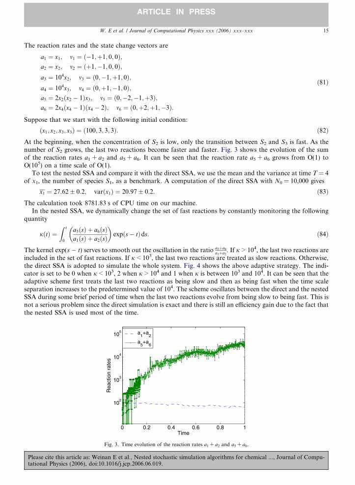
At the beginning, when the concentration of S2 is low, only the transition between S2 and S3 is fast. As thenumber of S2 grows, the last two reactions become faster and faster. Fig. 3 shows the evolution of the sumof the reaction rates a1 + a2 and a5 + a6. It can be seen that the reaction rate a5 + a6 grows from O(1) toO(105) on a time scale of O(1).

To test the nested SSA and compare it with the direct SSA, we use the mean and the variance at time T = 4of x1, the number of species S1, as a benchmark. A computation of the direct SSA with N0 = 10,000 gives

x1 ! 27:62+ 0:2; var#x1$ ! 20:97+ 0:2: #83$

The calculation took 8781.83 s of CPU time on our machine.In the nested SSA, we dynamically change the set of fast reactions by constantly monitoring the following

quantity

j#t$ !Z t

0

a5#s$ % a6#s$a1#s$ % a2#s$

! "exp#s& t$ds: #84$

The kernel exp(s & t) serves to smooth out the oscillation in the ratio a5%a6a1%a2

. If j > 104, the last two reactions areincluded in the set of fast reactions. If j < 103, the last two reactions are treated as slow reactions. Otherwise,the direct SSA is adopted to simulate the whole system. Fig. 4 shows the above adaptive strategy. The indi-cator is set to be 0 when j < 103, 2 when j > 104 and 1 when j is between 103 and 104. It can be seen that theadaptive scheme first treats the last two reactions as being slow and then as being fast when the time scaleseparation increases to the predetermined value of 104. The scheme oscillates between the direct and the nestedSSA during some brief period of time when the last two reactions evolve from being slow to being fast. This isnot a serious problem since the direct simulation is exact and there is still an e!ciency gain due to the fact thatthe nested SSA is used most of the time.

0 0.2 0.4 0.6 0.8 1

102

103

104

105

Time

Rea

ctio

n ra

tes

a1+a

2

a5+a

6

Fig. 3. Time evolution of the reaction rates a1 + a2 and a5 + a6.


ARTICLE IN PRESS


To test the nested SSA, we conduct a series of simulations in which the size of the ensemble and simulationtime of the inner SSA in the nested SSA scheme are chosen to be

#N ; T f$ ! #1; 2k * 10&5$; #85$

for di"erent values of k = 0, 1, 2, . . .. The error should be

k ! O#2k=2$: #86$

Table 4 gives the CPU time and the values of the mean and variance of x1 using N0 = 10,000. The sum of therelative errors of the mean and the variance is shown in Fig. 5.

0 1 2 3 4

0

0.5

1

1.5

2

Time

Fig. 4. Adaptive mechanism of the nested SSA.

0 1 2 3 4 5 610

–3

10–2

10–1

k

Fig. 5. Accuracy of the adaptive nested SSA.

Table 4E!ciency and accuracy of the adaptive nested SSA

Tf/10&5 1 2 4 8 16 32 64

CPU 13.6 18.6 28.0 47.2 86.2 163.0 316.2x1 27.50 27.55 27.44 27.51 27.55 27.55 27.61var(x1) 20.58 20.65 20.82 20.57 20.84 20.58 21.01


ARTICLE IN PRESS


The strategy for adaptively determining the set of fast and slow reactions may not be the best one. Furtherwork in this direction is clearly needed.

5. Nested SSA for systems with multiple time scales

Now we discuss chemical kinetic systems with multiple (more that two) well separated time scales. For sim-plicity, we focus on the instance when there are only three di"erent time scales. The general case can be studiedsimilarly. We will provide the asymptotic analysis for the e"ective dynamics on slow time scales and presentthe modified nested SSA for systems of this type.

5.1. E!ective dynamics for systems with multiple time scales

Suppose we are given a chemical kinetic system with R = {(aj,mj)} in which the rates aj(x) fall into threegroups: One group corresponding to the ultra-fast processes with rates of order 1/!2; one group correspondingto fast processes with rates of order 1/!; and one group corresponding to slow processes with rates of order 1:

a#x$ ! as#x$; 1!af#x$; 1

!2auf#x$

! ": #87$

The corresponding reactions and the associated state change vectors can then be grouped accordingly:

Rs ! f#as; ms$g; Rf ! 1

!af ; mf

! "; Ruf ! 1

!2auf ; muf

! ": #88$

The backward Kolmogorov equation for the observable u#x; t$ ! Exf #X t$ is then of the form:

ouot

! L0u%1

!L1u%

1

!2L2u; #89$

where L0, L1/! and L2/!2 are the generators of the Markov processes associated with Rs, Rf and Ruf. As before,

we can define a set of variables y which are slow compared with ultra-fast processes and are independent linearfunctions conserved during the ultra-fast reaction Ruf. As in Section 2.2, we shall denote these variables by

yj ! bj ( x #90$

where (b1, . . . ,bJ) are a basis of the subspace of vectors such that b ( mufj ! 0 for all mufj . Similarly, we can nowdefined slow variables z compared to both the fast and ultra-fast reaction as being independent linear func-tions conserved during the fast and ultra-fast reactions (Rf,Ruf). It is convenient to define the z variables aslinear combinations of the y:

zj ! cj ( y #91$

where (c1, . . . ,cK) are a basis of the subspace of vectors in RJ such that c ( !mfj ! 0 for all !mfj ! #b1 ( mfj; . . . ; bJ ( mfj$.To derive the e"ective dynamics, let us expand u as

u ! u0 % !u1 % !2u2 % ( ( ( ; #92$

and insert this expansion in (89). This leads to

L2u0 ! 0;

L2u1 ! &L1u0;

L2u2 ! ou0ot & L1u1 & L0u0:

8><

>:#93$

The first equation means that u0 belongs to the null-space of L2, i.e. u0#x; t$ ! U#b ( x; t$ for some U#y; t$ yet tobe determined. Inserting this expression into the second equation in (93) and looking for the solvability con-dition for the resulting equation, we arrive at

0 ! PL1U !XM f

i!1

!afi #y$ U#y % !mfi $ & U#y$) *

: #94$


ARTICLE IN PRESS


Here !mfi ! b ( mfi and

!afi #y$ !X

x2Xafi #x$ly#x$: #95$

where ly(x) is the equilibrium distribution of the fast process on the ergodic component indexed by y. (94)implies that U belongs to the null-space of the following generator defined on function f : Y ! R:

#L1f $#y$ !XM f

i!1

!afi #y$ f #y % !mi$ & f #y$# $: #96$

Assuming that the corresponding process generated by L1 is ergodic, with ergodic component indexed by z, i.e.it means that U#y$ is in fact a function of z = c Æ y, i.e.

U#y; t$ ! U#c ( y; t$; #97$

for some U#z; t$ to be determined. Let us denote by !lz#y$ the equilibrium distribution of the process generatedby (96) on the ergodic component indexed by z. Associated with lz(y) there is a projection operator Q definedas follows: for any v : Y ! R, it gives Qv : Z ! R as

#Qv$#z$ !X

y2Y!lz#y$v#y$: #98$

The equation for U is obtained from the solvability condition for the third equation in (93), which is obtainedby projection this equation first by P, then by Q. It reads

oUot

! QPL1U !XM s

i!1

!!asi#z$ U#z% !msi $ & U#z$% &

: #99$

Here !!msi ! c ( #b ( msi$ and!!asi #z$ !

X

y2X

X

x2Xasi #x$ly#x$!lz#y$: #100$

Notice that (99) is equivalent to following equation for !!u#x; t$ on the original state-space X,

o!!uot

!XM s

i!1

!!asi#c ( #b ( x$$ !!u#x% msi $ & !!u#x$) *

#101$

in the sense that if we solve (101) with the initial condition !!u#x; t ! 0$ ! f #c ( #b ( x$$, then !!u#x; t$ !U#c ( #b ( x$; t$ where U solves (99) with the initial condition U#z; t ! 0$ ! f #z$. We will make use of (101)in the following section. Notice also what we did above is an iterated averaging, a technique that has beendeveloped in the context of homogenization [1].

5.2. Multi-level nested SSA

When the assumptions for iteratively averaged dynamics (101) hold, we can generalize the nested SSA withtwo levels proposed in Section 3 straightforwardly to handle multi-scale system (88) by using a nested SSAwith more than two levels. Here we consider three levels. The innermost SSA uses only the ultra-fast ratesand serves to compute the averaged fast and slow rates using formulas similar to (37). This will give us thedynamics on the ultra-fast time scale and the following quantities

~as - Pas; ~af - Paf : #102$

The inner SSA uses only the above averaged fast rates ~af and the results are used again to compute the aver-aged slow rates (which are already averaged with respect to the ultra-fast reactions) as in (37):

as - QPas: #103$


ARTICLE IN PRESS


Finally, the outer SSA uses only the above averaged slow rates. The cost of such a nested SSA is independentof !, and as before, precise error estimates can be given in the same form of (41) in terms of Tuf – (the timeinterval over which the Innermost SSA is run and #~as; ~af$ is averaged), Nuf (the number of replicas in the Inner-most SSA), Tf (the time interval over which the Inner SSA is run and as is averaged), and Nf (the number ofreplicas in the Inner SSA):

error 6 C !% 1

1% T f=!% 1

1% T uf=!2% 1(((((((((((((((((((((((((((

N f#1% T f=!$p % 1((((((((((((((((((((((((((((((((

N uf#1% T uf=!2$p

!

: #104$

Let us take a look at an example. Consider the following system

S1 ¢a1

a2S2; S2 ¢

a3

a4S3; S3 ¢

a5

a6S4: #105$

with the reaction rates and state change vectors

a1 ! 2* 1010x1; m1 ! #&1;%1; 0; 0$;a2 ! 1010x2; m2 ! #%1;&1; 0; 0$;a3 ! 105x2; m3 ! #0;&1;%1; 0$;a4 ! 2* 105x3; m4 ! #0;%1;&1; 0$;a5 ! x3; m5 ! #0; 0;&1;%1$;a6 ! x4; m6 ! #0; 0;%1;&1$:

#106$

In this system, the first isomerization is ultra-fast, the second one is fast, the third one is slow, and ! = 10&5.The fast variables conserved during ultra-fast reactions are

#y1; y2; y3$ ! #x1 % x2; x3; x4$: #107$

The slow variables conserved during fast and ultra-fast reactions are

#z1; z2$ ! #y1 % y2; y3$ ! #x1 % x2 % x3; x4$: #108$

For each fast variable y, the ultra-fast reaction has an equilibrium distribution:

ly#x1; x2$ !y1!

x1!x2!#1=3$x1#2=3$x2dx1%x2!y1dx3!y2dx4!y3 : #109$

So the e"ective rates on the fast time scale are

!af3 ! P #105x2$ !2* 105

3y1; !mf3 ! #&1;%1; 0$;

!af4 ! P #105x3$ ! 2* 105y2; !mf4 ! #%1;&1; 0$:#110$

For each slow variable z1, the above reaction admits a unique equilibrium in the space of fast variable y:

!lz#y1; y2$ !z1!

y1!y2!#3=4$y1#1=4$y2dy1%y2!z1dy3!z2 : #111$

The e"ective rates on the slow time scale are:

!!as5 ! QP #x3$ ! Q#y2$ !z14; !!ms5 ! #&1;%1$;

!!as6 ! QP #x4$ ! Q#y3$ ! z2; !!ms6 ! #%1;&1$:#112$

Suppose that we take the total number of molecules in the system to be N = 1. Then when the whole system isat equilibrium on the slow timescale, the overall equilibrium distribution is

l ! #:2; :4; :2; :2$: #113$


ARTICLE IN PRESS


To test the convergence and e!ciency of the nested SSA, we take the following initial values

#x1; x2; x3; x4$ ! #1; 0; 0; 0$; #114$

and run the nested SSA to some long time on the slow time scale, say T = 104 using the parameters:

#N f ;Nuf ; T f ; T uf$ ! #1; 1; 10&2; 10&7$: #115$

We estimate the average equilibrium values of xi by recording the visiting frequency of the states. With theabove parameters, we obtain the following results:

l ! #:1999; :3994; :1991; :2017$: #three-level nested SSA$ #116$

The maximum error is about 0.0085 compared with the exact values given by (113). In contrast, it is almostimpossible to run the direct SSA to T = 104. To compare the e!ciency of the nested SSA with the direct SSA,we fix the total number of iterations in the calculations. The calculation with the nested SSA with the param-eters in (115) requires O(1010) iterations. With the same number of iterations, the direct SSA only advanced upto time T 0

0 ! O#1$, which is way too small to produce an accurate estimate for the equilibrium distribution.Fig. 6 shows this result. It can be seen that result from direct SSA is far from being accurate.

5.3. Nested SSA for the di!usive limit

In this section, we discuss the situation where the following centering condition holds

PL1U ! 0; #117$

which means that (94) is trivially satisfied. In this case, there is no need to introduce z variable as the slowdynamics on the O(1) time scale involves the y variables themselves. If (117) is satisfied, the second equationin (93) can be formally solved as

u1 ! &L&12 L1U : #118$

Inserting this expression into the third equation in (93), and looking for the solvability condition for the result-ing equation, we arrive at the following equation for U :

oUot

! PL0U & PL1L&12 L1U : #119$

The generators at the left hand side of this equation can be expressed more explicitly. The first one is simply

PL0U !XM s

j!1

!asj#y$ U#y % !msj; t$ & U#y; t$% &

; #120$

x1 x2 x3 x4

0

0.2

0.4

0.6

0.8

1

Em

piric

al d

istr

ibut

ion

Nested SSA

Direct SSA

Fig. 6. Empirical distributions obtained by nested SSA and direct SSA at the same cost. The distribution produced by nested SSA is nearlyexact, whereas the one produced by direct SSA is totally inaccurate.


ARTICLE IN PRESS


where !msj ! b ( msj and

!asj#y$ !X

x2Xasj#x$ly#x$: #121$

As for the second term in (119), let us denote by X ufx;t a sampling path of the process involving only the ultra-fast

reactions associated with L2 starting from x. Then for any v : X ! R such thatP

x2Xv#x$ly#x$ ! 0, we have

#&L&12 v$#x$ !

Z 1

0

#eL2tv$#x$dt !Z 1

0

E v#X ufx;t$dt: #122$

Using this expression together with condition (117), after some algebra one arrives at

&PL1L&12 L1U !

XM f

j!1

Aj#y$ U#y % !mfj; t$ & U#y; t$% &

; #123$

where !mfj ! b ( mfj and

Aj#y$ !X

x2Xly#x$

XM f

i!1

afi #x$Z 1

0

E afj#Xufx%mfi ;t

$ & afj#Xufx;t$

% &dt: #124$

(119) is equivalent to the following equation for !u#x; t$ on the original state-space X

o!uot

!XM s

j!1

!asj#b ( x$ !u#x% msj; t$ & !u#x; t$% &

%XM f

j!1

Aj#b ( x$#!u#x% mfj; t$ & !u#x; t$$; #125$

in the sense that the solution of (125) with the initial condition !u#x; 0$ ! f #b ( x$ is U#y; t$, the solution of (119)with the initial condition U#y; 0$ ! f #y$. (125) is a chemical kinetic system with the following reactionchannels

R ! ##!as; ms$; #A; mf$$: #126$

Based on the e"ective dynamics (125), a nested SSA for di"usive limit can be formulated. The nested SSA stillconsists of two levels of SSA. The inner level runs the ultra-fast reactions and the outer level runs the fast andslow reactions with modified rates estimated from the ultra-fast simulations using the following estimator for!asj and Aj:

~asj !1

N

XN

k!1

1

T uf

Z T uf

0

asj X ks

) *ds;

~Aj !1

N

XN

k!1

1

T uf

Z T uf

0

XM f

i!1

afi #Xks$Z T 0

uf

0

afj Y ks%x

) *& afj#X

ks%x$

% odxds;

#127$

where #X ks; Y

k;is%x$ is the kth replica of the virtual ultra-fast process Ruf with initial values X k

s!0 ! Xn (the currentstate in the e"ective dynamics) and Y k;i

0 ! X k0 % mfi . T

0uf is the virtual time we use to truncate the integral in

(122). We can also obtain an error estimate for this scheme:

error 6 C !% 1

1% T uf=!2% 1(((((((((((((((((((((((((((

N#1% T f=!2$p % e&aT 0

uf=!2

!

: #128$

For an explicit example, consider the following system

S1 ¢a1

a2S2; S2 !

a3 S3: #129$

with the reaction rates and state change vectors

a1 ! 105x1; m1 ! #&1;%1; 0$;a2 ! 1010x2; m2 ! #%1;&1; 0$;a3 ! 105x2; m3 ! #0;&1;%1$:

#130$


ARTICLE IN PRESS


For the above system, L0 = 0 and ! = 10&5. We can eliminate variable x1 by the conservation of the total num-ber of molecules x1 + x2 + x3 =M0 hence the ultra-fast variable is (x2,x3). The fast variable that keeps con-stant in the ultra-fast reaction is y1 = x3. The equilibrium distribution of x2 for the virtual ultra-fast process isthat of a one direction birth-death process such that

Prob#x2 ! 0$ ! 1: #131$

The action of P is then simply taking x2 = 0. The solvability condition (117) is satisfied since

PL1U ! P #x1#U#y1; t$ & U#y1; t$$ % x2#U#y1 % 1; t$ & U#y1; t$$$ ! 0: #132$

The solution of &L2v = x2 is v ! &L&12 x2 ! x2, which leads to

A3#y$ ! P #M0 & x2 & x3$ ! M0 & y1: #133$

Thus the only reaction channel in the di"usive limit is

R ! #M0 & x3; m3$; #134$

which is also a one direction birth-death process. For the nested SSA, we choose the parameters:

#N ; T uf ; T 0uf$ ! #1; 2* 10&9; T extinct$; #135$

where T 0uf ! T extinct means x2 is run till extinction in the ultra-fast simulation. Fig. 7 shows the time evolution

of the slow variable x3 on the slow time scale obtained by the nested and direct SSA simulations. The meanrelative error for the nth jumping time of x3 is less than 0.067. The computation of the direct SSA takes 131.2 sof CPU time while the nested SSA takes only 0.37 s.

6. Conclusion

We analyzed a nested stochastic simulation algorithm proposed in [7] for multi-scale chemical kinetic sys-tems. Convergence and e!ciency are proved and illustrated through examples. Generalizations to systemswith dynamic partition and multiple time scales of the fast and slow reactions are discussed.

Acknowledgments

The work of E is partially supported by NSF via Grant DMS01-30107. Liu is partially supported by NSFvia Grant DMS97-29992. Vanden-Eijnden is partially supported by NSF via Grants DMS02-09959 andDMS02-39625. We thank Princeton Institute for Computational Science and Engineering (PicSCie) for pro-viding the computing resources.

0 1 2 3 4 5 6 7 8 90

500

1000

1500

2000

2500

Time

x 3

Nested SSADirect SSA

Fig. 7. Time evolution of the slow variable y1 = x3 on the di"usive timescale.


ARTICLE IN PRESS


References

[1] A. Bensoussan, J.-L. Lions, G.C. Papanicolaou, Asymptotic analysis for periodic structuresStudies in Mathematics and ItsApplications, vol. 5, Elsevier, North-Holland, New York, 1978.

[2] A.B. Bortz, M.H. Kalos, J.L. Lebowitz, A new algorithm for Monte Carlo simulation of Ising spin systems, J. Comp. Phys. 17 (1975)10–18.

[3] Y. Cao, D. Gillespie, L. Petzold, The slow scale stochastic simulation algorithm, J. Chem. Phys. 122 (2005) 014116.[4] Y. Cao, D. Gillespie, L. Petzold, Multiscale stochastic simulation algorithm with stochastic partial equilibrium assumption for

chemically reacting systems, J. Comp. Phys. 206 (2005) 395–411.[5] W. E, B. Engquist, X. Li, W. Ren, E. Vanden-Eijnden, The heterogeneous multiscale method: A review, preprint, 2005.[6] W. E, D. Liu, E. Vanden-Eijnden, Analysis of multiscale methods for stochastic di"erential equations, Comm. Pure Appl. Math. 58

(2005) 1544–1585.[7] W. E, D. Liu, E. Vanden-Eijnden, Nested stochastic simulation algorithm for chemical kinetic systems with disparate rates, J. Chem.

Phys. 123 (2005) 194107.[8] B. Engquist, Y.-H. Tsai, The heterogeneous multiscale methods for a class of sti" ODEs, Math. Comp. 74 (2005) 1707–1742.[9] N. Fedoro", W. Fontana, Small numbers of big molecules, Science 297 (2002) 1129–1131.[10] D.T. Gillespie, A general method for numerically simulating the stochastic time evolution of coupled chemical reactions, J. Comp.

Phys. 22 (1976) 403–434.[11] D.T. Gillespie, Exact stochastic simulation of coupled chemical reactions, J. Phys. Chem. 81 (1977) 2340–2361.[12] E. Hairer, G. Wanner, Solving ordinary di"erential equations II: sti" and di"erential-algebraic problems, second ed. Springer Series in

Computational Mathematics, Springer, 2004.[13] E.L. Haseltine, J.B. Rawlings, Approximate simulation of coupled fast and slow reactions for stochastic kinetics, J. Chem. Phys. 117

(2002) 6959–6969.[14] R.Z. Khasminskii, On stochastic processes defined by di"erential equations with a small parameter, Theory Prob. Appl. 11 (1966)

211–228.[15] R.Z. Khasminskii, A limit theorem for the solutions of di"erential equations with random right-hand sides, Theory Prob. Appl. 11

(1966) 390–406.[16] R.Z. Khasminskii, G. Yin, Q. Zhang, Constructing asymptotic series for probability distributions of Markov chains with weak and

strong interactions, Quart. Appl. Math. 55 (1997) 177–200.[17] T.G. Kurtz, A limit theorem for perturbed operator semigroups with applications for random evolutions, J. Funct. Anal. 12 (1973)

55–67.[18] S.P. Meyn, R.L. Tweedie, Stability of markov processes, I, II, and III, Adv. Appl. Prob. 24 (1992) 542–574, and 25, 518–548, 1993.[19] G.C. Papanicolaou, Introduction to the asymptotic analysis of stochastic di"erential equations, in: R.C. DiPrima (Ed.), Lectures in

Applied Mathematics, vol. 16, American Mathematical Society, Providence, R.I., 1977.[20] C.A. Petri, Kommunikation mit Automaten, Institut fur Instru- mentelle Mathematik, Bonn, Schriften des IIM Nr. 2, 1962.[21] R.D. Present, Kinetic Theory of Gases, McGraw-Hill, 1958 (Chapter 8).[22] C.V. Rao, A.P. Arkin, Stochastic chemical kinetics and the quasi-steady-state assumption: application to the Gillespie algorithm, J.

Chem. Phys. 118 (2003) 4999–5010.[23] A. Samant, D.G. Vlachos, Overcoming sti"ness in stochastic simulation stemming from partial equilibrium: a multiscale Monte Carlo

algorithm, J. Chem. Phys. 123 (2005) 144114.[24] R. Srivastava, L. You, J. Summers, J. Yin, Stochastic vs. deterministic modeling of intracellular viral kinetics, J. Theor. Biol. 218

(2002) 309–321.[25] K. Takahashi, K. Kaizu, B. Hu, M. Tomita, A multi-algorithm, multi-timescale method for cell simulation, Bioinformatics 20 (2004)

538–546.[26] E. Vanden-Eijnden, Numerical techniques for multiscale dynamical systems with stochastic e"ects, Comm. Math. Sci. 1 (2003) 385–

391.


ARTICLE IN PRESS


nested stochastic simulation algorithms for chemical ...eve2/nssa_jcompphys.pdf · nested...

Documents