NBER WORKING PAPER SERIES

FREIGHT RATES AND PRODUCTIVITY GAINS IN BRITISH TRAMP SHIPPING 1869-1950

Saif I. Shah MohammedJeffrey G. Williamson

Working Paper 9531http://www.nber.org/papers/w9531

NATIONAL BUREAU OF ECONOMIC RESEARCH1050 Massachusetts Avenue

Cambridge, MA 02138February 2003

We are grateful for the advice given by Knick Harley, Michael Murray and Kevin O’Rourke, as well as fordata from David Hummels. Williamson also acknowledges with pleasure financial support from the NationalScience Foundation SES-0001362. The views expressed herein are those of the author and not necessarilythose of the National Bureau of Economic Research.

©2003 by Saif I. Shah Mohammed and Jeffrey G. Williamson. All rights reserved. Short sections of text notto exceed two paragraphs, may be quoted without explicit permission provided that full credit including©notice, is given to the source.

Freight Rates and Productivity Gains in British Tramp Shipping 1869-1950Saif I. Shah Mohammed and Jeffrey G. WilliamsonNBER Working Paper No. 9531February 2003JEL No. F1, N7, O3

ABSTRACT

The standard source for pre-WWII global freight rate trends is the Isserlis British tramp

shipping index. We think it is flawed, and that its sources offer vastly more information than the

Isserlis aggregate contains. The new data confirm the precipitous decline in nominal freight rates

before the World War I, but it also extends the series to the 1940s. Furthermore, our new series is

linked to the post-World War II era (documented by David Hummels), so that we can be more

precise about what has happened over the very long run. We also create route-specific deflators by

using the prices of commodities transported. Previous scholars have deflated their nominal freight

rate indices by a price index that includes tradables not carried on all routes and non-tradables not

carried on any route. Our deflated indices offer a more effective measure of the contribution of

declining freight rates to commodity-price convergence across trading regions. Using the pricedual

method and new indices for factor prices, we then calculate total factor productivity growth pre-war

and interwar for five global routes. Finally, we identify the sources of the total factor productivity

growth.

Saif I. Shah Mohammed Jeffrey G. WilliamsonCornerstone Research Department of EconomicsBoston, MA 02115 Harvard Universitysaifism@post.harvard.edu Cambridge, MA 02138

and NBER and Center for International Developmentjwilliam@kuznets.fas.harvard.edu

- 1 -

I. Introduction

The period between 1850 and the First World War saw increasingly integrated global

commodity markets. Economists commonly use the trade-to-GDP share to demonstrate this trend

(Maddison 1995), but this index can be very misleading. After all, outward shifts in import

demand or export supply can also lead to trade expansion even in an anti-global policy

environment. A better measure is the narrowing of price differentials between markets. That pre-

war agricultural and non-agricultural prices did indeed converge within Atlantic markets, within

non-Atlantic markets, and between them has been shown in a number of recent works (Harley

1980; O’Rourke and Williamson 1999; Williamson 2002; Findlay and O’Rourke 2002). While

integration was hindered by tariff barriers, world markets were far better integrated just before the

First World War than ever before.

Economists have mistakenly concentrated on trade policy to explain this globalization

trend prior to the First World War. Albert Imlah (1958), for example, started his account of Pax

Britannica by attributing the world trade boom to British leadership in adopting a liberal trade

policy, and historical accounts have always laid great emphasis on the repeal of the Corn Laws in

1846. Indeed, that date has often been designated as a marker for the beginning of a free trade

movement as liberal trade policies spread across Europe. However, the movement met resistance

after the 1870s as countries on the Continent retreated from openness, and tariffs were raised to

far higher levels in the European periphery, Latin America and the rich English-speaking

offshoots (Coatsworth and Williamson 2002). Bairoch (1989: pp. 55-8) and others have shown

that the rise in European tariffs was a defensive response to competition in local markets

increasingly integrated into world markets by a fall in transport costs on land due to railroads and

on sea due to shipping.

- 2 -

This paper focuses on the developments in the British tramp shipping industry up to the

Second World War. There is already enough published material to show that freight rates

declined precipitously before the First World War (Isserlis 1938; North 1958, 1965, 1968;

Stemmer 1989; Harley 1980, 1988, 1989; Fischer and Nordvik 1986; Yasuba 1978). This paper

fills in some of the gaps from a well-known source (Angiers) that has been incompletely mined. It

also replaces the famous but, we think, flawed Isserlis (1938) global tramp shipping index, the

standard source on global freight rate trends. In addition, the paper also fills a gap in the shipping

literature for the 1920s, 1930s and 1940s, decades that saw policy-induced de-globalization.

Finally, our global index is linked to that of David Hummels (1999) on shipping freights in the

post-World War II era, so that we can say something about the very long run.

We also create route-specific deflators by using the prices of commodities transported on

the route. Previous scholars have deflated their nominal freight rate indices by the Sauerbeck-

Statist British price index, an index that includes tradables not carried on all routes and non-

tradables not carried on any route. Our deflated indices offer a more effective measure of the

contribution of declining freight rates to commodity-price convergence across trading regions.

The first half of this paper documents our new freight rate indices for the period between

1869 and 1950. The second half explores the sources of that decline. This is a debate with an

impressive pedigree. Douglass North’s (1958, 1968) productivity gains calculations in shipping

surprisingly revealed that larger productivity gains took place before the introduction of the major

shipping innovations of the 19th century. North thus concluded that improvements in management

and industrial organization drove the fall in freight rates, and that technological change was only

secondary. Knick Harley (1988) challenged this long-accepted view by showing that there were

significant problems with the North freight rate index. Basically, the early part of the 19th century

saw a sharp decline in the stowage factor (i.e. space occupied per ton) of cotton. The packing of

cotton bales improved considerably with the introduction of the screw press followed by the

steam press, both allowing more cotton to be crammed into holds (Harley 1988: pp. 856-9). This

- 3 -

led to a steep fall in cotton freight rates in the first half of the 19th century. Since North’s freight

rate index was heavily weighted by cotton, it did not represent general shipping trends.

Conducting a productivity gains calculation on a revised index, Harley concluded that the more

significant productivity gains took place after 1869, and were attributable to the introduction of

the steam engine and improvements in hull technology. The conventional history was reclaimed.

While Harley appeared to have settled one debate,1 he created another by noting that the

shipping industry was marked by joint-production on different legs of journeys (Harley 1985;

1988; 1989; 1990). Calculating TFP gains without taking into account joint-production could lead

to a significant measurement bias the size and direction of which would depend on the shipping

route. After analyzing the joint-production issue, we revisit Harley’s measurement of TFP gains

between 1870 and 1896. Using the price-dual method and new indices for factor prices, we

calculate productivity gains for this period anew, not only for the Bombay-UK route examined by

Harley but also for four other routes. We then move on to calculate TFP growth for the period

between the early 1890s and the First World War, as well as that between the two World Wars,

the latter having received relatively little attention in the shipping literature.2 Finally, we explore

the sources of that productivity experience.

1 Harley has not been alone. Yasukichi Yasuba (1978) calculated productivity gains in Japanese pre-WWIItramp and liner shipping using quantities of outputs and inputs, and Walter Knauerhause (1968) did thesame for labor productivity on German liners in the 1870s and 1880s.2Data limitations force us to restrict our calculations to the British tramp shipping industry, almost entirelyignoring the liner shipping industry. Liners, unlike tramps, operate on fixed time schedules on fixed routes.Tramps are hired to carry either restricted (i.e. specified in the contract) or unrestricted cargoes betweennegotiated ports, and unless a fixed time charter is negotiated, no time schedule or route is fixed. Trampshipping dominated trade in commodities. In 1909, a Royal commission found that tramps made up 70-80% of total tonnage, so that liners could not have been more than one-third of the total (Pollard andRobertson 1979: p. 20). Liners did not operate on full capacity, and carried high value articles that wereless bulky. Tramps carried the high bulk, low value staples.

- 4 -

II. Freight Rate Indices

The Need for New Indices

It is surprising that the Isserlis global freight rate index has remained the standard source

on global freight rates for 1869-1936 given that its construction is flawed. The flaws are more

than those pointed out by Yasukichi Yasuba who argued that there is an upward bias in the

Isserlis index since “declining rates were quoted only after the number of contracts reaches a

certain level, and rising rates for the old established routes tend to remain in the list longer than

they deserve” (Yasuba 1978: p. 13). Isserlis took his data from Angier’s annual reports on British

shipping, and it is true that Angier’s choice of which freight rates to report was somewhat ad hoc.

The more troubling problem with the Isserlis index, however, lies with the way the data were

aggregated3 and with the deflator used to convert from nominal rates. We think it is time to return

to Isserlis’ original source and reconstruct the global index.

The Angier Data

Isserlis reports in an appendix the ratio of the simple average of the highest and lowest

freight rates for a commodity-route in that year to the same average for that commodity-route in

the immediately previous year. This ratio is not available for all routes and for all years, and the

number of gaps in the Isserlis data far outnumber the number of observations. In fact, for almost

every commodity-route, it is impossible to judge the level of freight rates relative to 1869. To do

so, we would need the nominal freight rates themselves, and while they are not in Isserlis, they

can be found in Isserlis’ sources. The Angier annual reports included tables of highest and lowest

British tramp shipping freight rates for various commodity-routes, and these were compiled in

3 Isserlis used Angier’s data to form the ratio of the freight rate on each commodity-route to the freight rateon that commodity-route in the immediately previous year. He then took the arithmetic average of allavailable freight rate ratios for each pair of years, using them to form his global freight chain index. He

- 5 -

Fifty Year Freights (Angier 1920). From the 1880s onwards, they were published annually in a

January edition of Fairplay magazine, a leading British shipping journal. While Isserlis stops

with 1936, the Angier-based freight index can be extended to 1950, which we do in this paper.

Furthermore, while the Angier reports end there, Fairplay included its own reports on tramp

shipping, at least until 1962. These data make it possible to link our index to the modern era

(Hummels 1999).

Mining these sources, we were able to find freight rates for over 500 commodity-routes

from all over the world, but mostly for trade between Europe and the rest of the world, on both

homeward and outbound routes. True to the nature of tramp shipping, the freight rates reported

are for low-value bulk commodities. Most of the rates were reported in shillings/pence per ton.4

Nowhere does Angier make clear why he decided to report certain commodity-routes,

though in some cases he does mention that not enough charter parties were reported to him to be

able to note the highest and lowest freight rates for the year. We are left to guess that Angier

reported only the commodity-routes he thought were important to British tramp shipping.

Finally, we note what Angier almost entirely left out: the short range trade between

Britain and continental Europe, and shipping between non-European ports. Thus, we cannot be

certain that any index based upon this database is representative of global shipping. At best, the

index documents trends in freight rates on bulk commodities between the European center and the

periphery.

rebased this chain index in a single year, 1869. There are significant problems with this method ofconstruction. See Appendix 1.4 There are over 8,000 observations. For some commodities, freight rates were reported per 40 cubic feet,though in early years, their freight rates were reported per ton. Where freight rates were not reported perton, we were able to turn to sources on stowage factors (i.e., the space occupied per ton) from the period tostandardize these freight rates. For some commodity-routes (particularly Black Sea grain routes, Newcastlecoal routes in the early years, or the timber routes, freight rates were reported in region-specific or trade-specific unites. These too were standardized by combing through Angier’s reports, the contemporaryshipping literature, and the Oxford dictionary.

- 6 -

Construction of the New Indices

Given that the commodity-routes included in Angier keep changing, and that the series

have intermittent gaps, it is impossible to aggregate these data directly to form an index of long

distance tramp shipping freight rates, but an indirect strategy seems to work: construct indices for

outbound and homeward trade between Europe and individual regions, and then aggregate these

indices into a final “global” index. These route indices are, of course, themselves useful for

analyzing the development of trade between various parts of the periphery and Europe.

Before describing the construction of these route indices, we need to say a word about a

technological constraint that must be taken into account in the construction of our freight indices.

Harley (1990: pp. 157-8) describes this best:

“Ships float by displacing water. Seawater weighs sixty-four pounds per cubic foot or

displaces thirty-five cubic feet per ton. Since the ship itself has some weight, cargoes

such as coal and heavy grain (wheat, rye and corn), which occupy forty cubic feet per

ton, simultaneously fill up a ship and exhaust its buoyancy. Light cargoes, such as cotton,

tend to leave a ship with excess buoyancy for optimal navigation. Consequently, a ship

carrying primarily cotton will be willing to take heavy cargoes at low rates. Alternatively,

a heavy cargo such as iron or ore will exhaust a ship’s buoyancy while it still has empty

space. If this is the primary cargo, then light cargo will be sought to fill available space,

and low rates will be offered.”

Thus, freight rates for commodities with different stowage factors behaved very differently, and

they responded very differently to changes in shipping technology. Because the tramp shipping

industry was competitive and because the time charter party was part of it (e.g. shippers could

take any commodity the ship would carry), freight rates for commodities with similar stowage

factors behaved similarly. Thus, we construct our regional indices from commodities with similar

stowage factors.

- 7 -

Our global index of long distance tramp freight rates between Europe and the rest of the

world is constructed weighting the different regional indices according to the importance of trade

to and from that region. We use the Board of Trade data (taken from Mitchell 1992) to compute

the ratio of trade to Britain being carried to the individual regions to the total trade carried to all

the regions in the database. These ratios formed the weights for the homeward routes. Outbound

coal freight indices for the various routes were weighted by the ratio of coal carried to these

regions to the total for all the regions in the database. The results are plotted in Figures 1A and

1B.5

Nominal Freight Rate Indices

The new freight rate indices confirm what has long been known about pre-First World

War shipping costs: nominal freight rates declined along all routes. In the interwar period,

however, freight rates recovered their low pre-war levels only in the mid-1930s, for reasons that

will be explored in the next section. Replacing the Isserlis index with our new Global Index

makes a difference. The new index (Figures 1A and 1B) falls faster than the Isserlis index before

and after 1884, suggesting that Isserlis understated the fall in freight rates. After the War, Isserlis

again understates the fall in global tramp freights.

Important differences in the behavior of tramp freights in different regions emerge when

the regional freight rate indices are examined. The Atlantic routes exhibit a wide variety across

different regions and commodities. Timber freights on the eastern North America and Baltic

routes fell much more slowly than did grain freights on the same routes before the First World

War. This is to be expected because of joint-production. Timber did not exhaust both buoyancy

and space, and thus could not take advantage of the increases in ship sizes that were to drive

5 Details on the construction of the route and “global” indices are supplied in Appendix 2.

- 8 -

productivity gains before the War. On the other hand, freight rates on ore carried from the

western Mediterranean, heavier than grain, fell as fast as rates for transatlantic grain cargoes.

Freight rates on grain from the Gulf Coast of North America (GNA) and the East Coast of North

America (ENA) seem to have followed each other closely, at least between 1884 and 1913,

falling by about 25-40% in this period. The fall in grain freights from ENA was slightly sharper

than that for GNA in this period. Baltic and ENA rates both fell by about 40% between 1874 and

1884, though Baltic freights fell more slowly thereafter. Freight rates for grain from East Coast of

Latin America (ELA) fell much slower than for either of these regions between 1869 and 1884,

barely dropping by 10% in this period. Between 1884 and 1913, however, the ELA grain index

matches the performance of GNA and ENA grain freight indices in this period. Freight rate series

for the west coast of North America (WLA: grain) and Latin America (WLA: nitrates) are also

presented in Table 1. These routes were dominated by sailing vessels. Rates fell steeply for the

WNA grain route before 1884. For WLA, however, freight rates fall only after 1884.

The behavior of Latin American freights cannot be explained by the diffusion of new

shipping technologies or distance. WLA, for example, was closer to Europe than WNA, and yet

rates fell faster for the latter route. Harley (1989: p. 327) remarks upon the complexity of the

relationship between outbound and inbound freights in Latin America. The next section examines

how freight rates on various legs of voyages were not determined independently. Demand for

inbound and outbound shipping fluctuated erratically for Latin America. Before 1884, coal

freights for the East Coast of Latin America were falling quicker than freights for coal carried to

most other regions (Table 1). Coal freights for ELA were certainly falling much faster than

outbound grain freights. The explanation for the behavior of Latin American freights likely lies

with shipping demand in these regions.

- 9 -

The First World War saw freight rates peak for the Atlantic routes. They fell only slowly

in the interwar period. It was only around 1933/4 that nominal freight rates fell to their pre-war

levels, but they rose again with the onset of the Second World War.

Coal freight rates (Table 1) do not seem to have been correlated with distance either.

Bombay coal freights, for example, fell much faster than Colombo coal freight rates before 1884,

even though Colombo was only slightly farther away from Britain than Bombay. Outbound coal

freights from Britain seem to have fallen drastically in the interwar period, unlike homeward

freight rates.

Homeward freight rates for non-Atlantic routes (Table 2) fell precipitously between 1869

and 1884. Particularly noteworthy were grain freights from Black Sea ports, that fell by over

60%. Freight rates for western Indian and Bay of Bengal ports fell by over 40% in this period.

Unlike timber on the Atlantic routes, freight rates on lighter commodities that did not exhaust

both buoyancy and space actually fared better that freight rates for commodities with stowage

factors similar to grain. Freight indices for lighter cargoes such as jute transported from the Bay

of Bengal fell by over 65%, although it is unclear how much of this fall was actually caused by

better packing. For Southeast Asia, where the diffusion of steam technology in shipping was

slower because of distance, freight rates fell much more slowly than for India. After 1884,

however, the freight indices for these routes mirror each other for similar types of commodities.

Freight rates fell by up to 25% before the First World War. As in the Atlantic homeward routes,

freight rates fell gradually from their wartime heights in the interwar period.

Real Freight Rate Indices

In order to deflate these nominal indices, we, like other scholars, turn first to the

Sauerbeck index. But the Sauerbeck index is imperfect for our purposes since it includes non-

tradables and many tradables not carried on all routes. As an alternative, we constructed route-

- 10 -

specific deflators by taking the unweighted average of the prices of the commodities included in

the commodity-routes. Both our preferred real indices and the Sauerbeck deflated indices are

discussed in Appendix 3.

Figures 2A and 2B illustrate the impact of the deflators by plotting both for two cases: the

American wheat trade and the Calcutta jute trade. The Calcutta nominal freight rate index

deflated by jute prices fell faster after 1873 than the same index deflated by Sauerbeck. Deflating

by Sauerbeck thus understates the fall in real transport costs. The difference is less pronounced in

the ENA-grain route, perhaps because wheat prices get a large weight in the Sauerbeck index.

Extending the Global Index to 1997

Looking at the modern era, David Hummels (1999) reports the Norwegian Shipping

News global freight rate index for tramp charters starting in 1947. Figure 3 and Table 3 use this to

link our series with that of Hummels, making it possible to plot global nominal freight rates for

the 127-year period between 1870 and 1997.6 The nominal freight rates seem to trace out a U-

shaped pattern: while the pre-World War I decades saw a continuous fall in nominal freight rates,

the trend was reversed during the war years; and while the pre-war nominal freight rates were

briefly recovered by the middle of the great depression, they have traced out a trend rise ever

since. However, these nominal series need to be deflated by commodity prices. We do so in

Figure 4 where the trend in real tramp freight rates is documented for over the 127-years. The

period between 1870 and 1914 saw an almost uninterrupted fall in shipping costs relative to the

prices of the commodities carried along almost all routes; the war and interwar years were ones of

great instability and little downward trend; and the half century since were years of stability and

no downward trend.

6 Appendix 2 explains exactly how these indices are linked.

- 11 -

Hummels (1999: p. 12) blames the post-World War II increase in nominal freight rates on

the rise in factor prices. The sharp rise in the 1970s (Figure 3) was, no doubt, related to the

dramatic quadrupling in oil prices at that time, but other major inputs also recorded a 10-30%

rise. A 1977 UNCTAD report claimed that even port costs were rising due to mushrooming labor

costs and other cost pressures (Hummels 1999: p. 13). Of course, tramp shipping had to deal with

rising input costs before 1950 too, and the real indices in Figure 4 are, after all, deflated by

commodity prices. The key, therefore, to long run trends in freight rates was and is total factor

productivity growth. Any retardation in the fall in freight rates plotted in Figure 4 must reflect a

slow down in the rate of productivity advance.

III. Total Factor Productivity Growth

The Problem of Joint Production

The assumption of long run Marshallian competitive equilibrium, whereby the average

freight charge is equal to the average cost of the journey, allowed North to write total factor

productivity growth as

A* = Pi* – Pf* = Q* – Qi* (3.1)

where A is total factor productivity, Pi is an index of factor prices weighted by factor shares, Pf is

the freight rate index, Q is the quantity index of outputs (i.e. amount of goods carried), and Qi is

an index of the quantities of various inputs weighted by factor input shares, and the * superscript

denotes rates of change.

North’s assumption is not unreasonable, given the competitive nature of tramp shipping.

The fact that shipping and ship building were relatively small players in the markets for labor,

capital, metal and machinery also supports the assumption that factor prices were exogenous to

this industry. However, and following Harley’s suggestions (1988; 1985; 1989; 1990), we depart

- 12 -

from North’s assumption that joint production along outward and homeward routes did not

matter. Since freight rates carried on each leg were often interdependent, average freight rates did

not always equal average total costs on individual legs of journeys. Productivity gains calculated

only on a single leg are likely, therefore, to be incorrect.

The existence of shipping capacity in one direction automatically creates shipping

capacity in the other since ships have to return to their homeports for repairs and to return their

crews. The simplest case is where demand and marginal cost are the same on both legs. Given the

competitive conditions of the tramp shipping industry on any route,

Ph = MCh = ATCh (3.2)

Po = MCo = ATCo (3.3)

where P is the freight rate, MC is the marginal cost of undertaking the voyage, ATC is the

average total cost for each unit space or weight of the carried good, h denotes the homeward

journey, and o the outbound journey. It is not necessarily true that the more full the ship, the

lower the average total cost. Filling a ship beyond a certain level may undermine stability or

increase the average fuel cost, and this level may be defined as full capacity. Of course, in

competitive equilibrium, ships would be filled to this full capacity. Given all of these

assumptions, freight rates in both directions would be equal, and to the marginal cost along each

leg.

Now suppose that the demand for shipping in the two directions is different, as would be

the marginal costs of the voyage. In the 19th and early-20th centuries, Britain was the primary

supplier of much of the world’s coal used as bunker fuel, and the cost of bunker coal thus

increased the farther one was from Britain. Fuel costs on the voyage back to Britain were higher

than on the outbound voyage. Marginal costs could also have been different because crew costs

were different in the two directions. Lewis Fischer (1989) has claimed that the markets for able-

bodied seamen in northern European ports were not well-integrated, and that seamen earned more

if they were hired at major ports, such as Liverpool. There is also ample evidence that Indian

- 13 -

seamen on British ships earned less than their European counterparts. Indian seamen formed a

substantial portion of the British shipping labor force, as high as 20%. Potentially, ships could

lower marginal costs by hiring in lower-wage ports en route to or at their destination. Likewise

ships and crewmembers could agree to part company at low-wage ports of call along the journey.

If freight rates in the two directions were determined separately, we would expect that

competitive pressures would have driven freight rates on each leg to the point where they would

equal marginal cost per unit space or weight (and average total costs) for that leg. The demand

and freight rate for shipping on the two legs would have been equal only by chance. Assuming

that the demand for shipping on the homeward leg exceeded the demand on the outbound leg, one

of two cases would have arisen, given that the supply of shipping in the both directions had to be

equal. If the entire demand for shipping on the homeward leg was met by supply (at some

competitive freight rate), then there would excess supply available on the outbound leg. Thus,

some, if not all, ships plying the homeward route would be filled to less than full capacity, and

the cost of carrying these goods would not be covered for these ships. In long run competitive

equilibrium, ships making losses would leave the route. Then, the entire demand on the

homeward route would not be met, and there would be a shortage of shipping space in the

outbound route. Alternatively, suppose the entire demand was supplied by shipping space on the

outbound route. In this case, there would be a shortage of shipping in the homeward direction,

and we would see shippers bidding freight rates up. Freight rates would exceed the marginal cost

of making that leg of the voyage. Thus ships on the homeward route would be making excess

profits.

However, barriers to entry on any route were insignificant in the long run. Ships setting

freight rates on the two legs jointly could still earn profits on the journey as a whole. If x were the

profit per unit earned by the ships on the homeward direction, a profit could be earned by setting

freight rates in the following manner:

Ph = MCh + ax a<1 (3.4)

- 14 -

Po = MCo - abx b<1 (3.5)

Ships setting freights separately would have to lower rates to get any cargo. Again, given

the absence of barriers to entry, ships could take away all business on the outbound route from

these ships charging rates according to (3.5) by further lowering the freight rate by setting a new

b, denoted b* such that 1<b*<b in equation 3.5. The argument can be repeated so that in the

competitive equilibrium, b will in fact equal 1. Thus Po = MCo – ax.

As long as demand for shipping in one direction is greater than demand in the other, ships

will continue to face inelastic demand on the voyage leg with greater demand. The argument

above can be repeated, until at the combination of rates Ph* and Po* where the demand in both

directions will be equal. By the argument here,

Ph* = MCh + x* (3.6)

Po* = MCo – x* (3.7)

Obviously, Ph* + Po* = MCh + MCo, which will be equal to the average total cost of the journey

taken as a whole. No profits are earned for the journey taken as whole and marginal costs on both

legs are just covered even though the freight rates do not equal marginal (and average total) costs

on either leg of the journey.

Finally, there is a possibility that demand on the outbound leg will be lower than demand

on the homeward route no matter what the freight rates are. When the freight rate is zero on the

outbound route, demand for shipping is infinite. Ships have the option of either taking the cargo

for free, or undertaking the outbound voyage in ballast. Since there are costs associated with

loading and unloading cargo, ships may prefer to travel in ballast, since loading and unloading

ballast was generally less expensive than handling cargo. If some ships do decide to take cargo on

the outbound route, freight rates for the outbound cargo would equal the average cost of

collecting, carrying and unloading them. Freight rates on the homeward cargo would equal the

average total cost of the roundtrip voyage less the marginal cost of carrying outbound cargo.

Total costs of the journey still equal total revenue.

- 15 -

Two minor adjustments complete the analysis. First, in the long run, owners will want to

use their ships with “optimal” qualities fitting the specification of the trade and the route so that

the cost of operation is minimized. Costs included the interest paid on the price of the ship.

Larger, faster and more specialized ships were more expensive to build. This tradeoff saw tramp

ship owners purchasing ships that were not entirely top-of-the-line, but of medium sizes and

moderate speeds, with few or no special fittings for particular trades. The ship-building industry,

itself an extremely competitive industry, contributed to this trend by churning out medium-sized

steamers in anticipation of demand, and these were sold at prices much lower than those of made-

to-order vessels (Pollard and Robertson 1979: p. 20). It was thus possible by the 1930s for the

tramp ship owner to describe an “ideal” tramp ship as a medium-sized, moderate speed

nondescript jack-of-all trades steamer with no special fittings for any particular type of trade

(Sturmey 1962: p. 35).

The second adjustment is only cosmetic, and it has to do with our assumption that all

ships originated from a single homeport. The competitive conditions still hold even if ships

originate at different homeports at the two ends of the shipping route, given the need for ships to

return to their origins. The sum of the freight rates on the different legs will still equal the sum of

marginal costs. Thus, changing this assumption would only require changing the wording of the

exposition here.

The analysis can of course be extended to journeys with more than one leg, as long as the

condition holds that the supply of shipping space in one leg implies a supply of shipping space in

another leg of the journey. Thus, economic profits on a tramp journey from Britain, dropping off

coal at Suez, traveling in ballast over the Red Sea and the Arabian Sea to Bombay, and traveling

back to Britain with a cargo of general goods would be zero in long run competitive equilibrium,

just as they would be zero if the coal were to be carried through Suez and dropped off in Bombay

instead. The freight rate on the homeward route from Bombay would have to be the same no

- 16 -

matter which route was taken to get there. The freight rate on coal to Suez and the average cost of

traveling in ballast from Suez to Bombay would have to equal the freight rate on coal to Bombay.

There was another kind of joint production relevant in this period (Harley 1990). Freight

rates were determined jointly not only on the different legs of the journey, but also for different

commodities carried on any single leg of a voyage. This jointness arose because of the disparity

between bulk and weight of different commodities and the limitations of navigational technology

in this period that required buoyancy to be filled.

Freight rate, and thus productivity gain, calculations should control for a mixture of

commodities as well as for a mixture of legs (Harley 1990: p. 158). Calculations of productivity

gains that do not take into account both types of jointness of production could be misleading. If

the index for a particular leg of a voyage were used in calculating productivity gains, and if

freight rates on that leg fell faster than freight rates on the journey taken as a whole, productivity

gains would be overstated. Similarly, if freight rates on the individual good fell much faster than

on other commodities, productivity gains would be overstated.

It is difficult to adjust for the second kind of joint production simply because the

interrelationships among different cargoes were so complex. Luckily, on the routes where freight

rates for different commodities were interrelated, we are often able to isolate time series of freight

rates that were determined independently. In the case of the North Atlantic trade, where joint

production of the second kind were particularly important, Angier’s data present us with a series

of charter party freight rates charged by tramp steamers that carried only grain to Europe. No

adjustment is necessary in this case for the second type of joint production. Our productivity

gains results for the Baltic, however, require the disclaimer that joint-production of grain freights

with timber freights were not taken into account.

The first type of joint production between different legs of the journey is easy to

accommodate. As our analysis above demonstrates, as long as there is no joint production of the

second type, the sum of freight rates per unit weight or space would equal the sum of marginal

- 17 -

costs of the different legs of the journey. Thus, even though the individual freight rates on

individual legs of the journey do not equal the marginal cost associated with undertaking the

voyage on that leg, freight rates on the voyage taken as a whole do equal the average total cost of

the voyage. We add outbound coal freights (per ton) to the freight rate (per ton) on the homeward

journey on that route for a commodity with stowage factors similar to grain. This sum should

equal the average total cost of the journey in long run competitive equilibrium.

Total Factor Productivity Growth

Harley (1988) calculates productivity gains on the UK-Bombay route for the outbound

coal trade and the inbound general goods trade and thus implicitly confronts the joint-production

problem raised above.7 First, we redid Harley’s calculations for the period between 1871-3 and

1887-9 using much improved factor price data, in particular new wage and coal price data

(Appendix 3). Second, we extended the calculations to 1909-11. Third, and in order to increase

generality, we added TFP growth measurements for three other routes – UK-East Coast of North

America, UK-Alexandria and UK-Riga – again using data for outbound coal freights and inbound

bulk commodities with stowage factors similar to that of grain. The pre-war TFP growth results

are summarized in Table 4.

Between 1871/3 and 1887/9, 50-65% of the fall in freight rates can be explained by the

decline in factor prices. Falling ship prices, driven by the introduction of cheap iron hulls and

productivity gains in the shipbuilding industry, resulted in around 25-35% of the fall in freight

rates. Productivity gains in the coal industry no doubt contributed to the fall in coal prices, but the

decline in shipping costs also meant that Welsh bunker coal picked up at non-British ports was

7 His TFP growth calculations are taken from his 1972 Ph.D. dissertation (although Harley does notmention joint-production in the thesis).

- 18 -

getting cheaper. Productivity gains in the shipping industry account for the rest of the fall in

freight rates (35-50%).

These productivity estimates differ from Harley’s. Harley estimates annual TFP growth

for the Bombay route between 1873/4 and 1890/1 to have been 3.1%, while we estimate a more

modest, and perhaps more plausible, 1.6%. Part of the difference can be attributed to the fact that

our freight rate index falls less steeply, and this fact can be explained mainly by his inclusion of

the unusual years 1874 and 1890 in the calculation. We elected to choose less unusual end point

years since 1874 saw freight rates spike upward to a half-decade high, while 1890 saw freight

rates collapse to their lowest.

Productivity growth rates on our other three sampled routes were lower than those on the

Bombay route. TFP growth along the ENA and Alexandria routes were the lowest of the four

presented in Table 4. The probable explanation is that these two routes had already absorbed the

new changes in steam technology and thus they are likely to have recorded higher TFP growth

rates in the 1860s and early 1870s; after all, steam technology was well established in the

transatlantic trade by the early 1870s. Alexandria also had been early in adopting the steamship

since the new technology was not susceptible to variable Mediterranean winds. In contrast, the

Bombay route introduced the steamship only with the construction of the Suez Canal in 1869.

Naturally, the adoption of the new technology saw higher subsequent productivity gains along the

route.

The Riga route, though closer to Britain, was slower in adopting the new shipping

technology than were either the ENA and Alexandria routes. The route had long been known as a

backwater for older and slower vessels, but the gap between the mean age of the British fleet and

the age of British ships in the Baltic was narrowing in the 1870s and 1880s, and by the start of the

1880s, the majority of the Baltic timber trade was carried on steamships (Fischer and Nordvik

1987: pp. 103-5). Thus steam technology came on in a rush during the 1870s and 1880s, and this

- 19 -

fact contributed to the rapid TFP gains along the Riga route, much like those along the Bombay

route.

Average export prices for British coal were increasing between 1887/9 and 1909/11, and

on the shorter routes such as the Baltic and the Mediterranean, coal freight rates did not fall

quickly enough to override the rise in “world” coal prices. The cost of bunker fuel at foreign ports

along these routes thus increased, retarding the fall in freight rates especially on the Riga and

Alexandria routes. For the ENA and Bombay routes, coal freights fell fast enough to overcome

the rise in “world” coal prices. Along the Bombay route, the fall in the price of bunker fuel

contributed to about 10% of the fall in freight rates. Along the ENA route, the effect of coal

prices was negligible.

Declining ship prices induced a similar fall in freight rates in both periods. During this

second period, however, there is also a wider variation of TFP growth among routes. Continued

high productivity in the Baltic can partially be explained by continued diffusion of steam

technology along the route: while other routes had gone over to steam almost entirely by the

1890s, about 20% of Baltic ships trading in timber were still powered by sail even at the turn of

the century (Fischer and Nordvik 1987: p. 105). For other routes, it is more difficult to make the

argument that these big productivity gains were a function of the diffusion of steam technology.

The old transatlantic route underwent an acceleration in TFP growth between 1871/3-1887/9 and

1887/9-1909/11, achieving TFP growth rates similar to those along the Bombay route, where

rates had been maintained.

The availability of outbound coal freight rates for Alexandria and North America make it

possible to extend these calculations up to 1932-4, immediately prior to the introduction of

government regulations in 1935 that aimed at limiting competition in tramp shipping (Sturmey

1962: p. 110). In order to exclude the effect of the First World War, we conduct two calculations:

the first is for the period between 1909/11 and 1932/4, and the second for the period between

1923/5 and 1932/4. The results are summarized in Table 5.

- 20 -

Factor prices jumped during the First World War, and even by 1923/5 wages, ship prices

and fuel prices were still about double those in 1909/11. Thus, even though post-war nominal

factor prices declined, they never recovered their pre-war levels in the 1920s. It was the inflated

factor prices that prevented freight rates from falling, not slow productivity advance. Indeed,

interwar TFP growth rates were at least as high as pre-war: TFP growth rates for ENA actually

doubled after 1909/11, those for Alexandria also rose, and only those for Bombay fell.

TFP growth rates between 1923/5 and 1932/4 were much smaller for all three routes than

they were between 1909/11 and 1932/4, implying that the First World War induced substantial –

but temporary -- improvements in productivity, no doubt due to full capacity demands in wartime.

IV. Explaining Productivity Gains

The revolution in shipping technology has been recounted many times (e.g. Pollard and

Robertson 1979: pp. 9-24). This revolution rested on two developments: the decrease in iron, and

later steel, prices that made economical the introduction of new metallic hulls in ship construction

in the second half of the 19th century, and the advances in engine technology that saw vast

increases in fuel efficiency. These changes were related to changes in the metallurgical, chemical

and engineering sciences that spilled over into the shipbuilding industry. The results were lower

ship prices for larger and faster ships allowing British firms to wrest leadership in shipping from

the Americans by the 1860s. Britain maintained this leadership unchallenged until the First World

War, when British ship owners rejected the more efficient diesel engine for the older, trusted

steam engine.

How did changes in shipping technology affect the industry? We are told (e.g. Pollard

and Robertson 1979) that iron and steel allowed for larger ships with bigger steam engines that

reduced coal consumption and increased speeds. These changes also made it possible to reduce

- 21 -

crew sizes, and to take advantage of economies of scale. Given all these benefits, why the big

differences in adoption and diffusion between routes?

We have the input data for the period between 1869 and 1913 that will help us seek

answers to these questions. Much of the data documenting the quantity of labor used, time spent

at sea and in port, the size of vessels and engines on various routes come from the impressive

Atlantic Canada Shipping Project (ACSP) dataset constructed at the Memorial University of

Newfoundland. The ACSP data come from the British Agreements and Accounts of Crews,

official documents that had to be filled by any British ship whenever a crewmember joined its

ranks. The data includes a 1% random sample of all voyages by British ships between 1863 and

1914. The rest of the pre-1890 data utilized here, particularly the coal consumption data mainly

come from Harley, and we have extended these series up to 1913 by scouring contemporary

shipping sources. We have much less information about the interwar period, though Sturmey’s

(1962) study of British shipping was quite useful.

Cargo Capacity (Hull Weight)

Using ship, steel and iron price data, Harley (1972: p. 311) estimates that average hull weight fell

by about 10% between 1870 and 1890. Pollard and Robertson (1979: p. 14) report that the

introduction of steel, largely after 1890, reduced hull weights by 15%. Most new ships

constructed on the Clyde in 1890 were made of steel. Allowing for the diffusion of steel in the

tramp shipping industry, as well as the slight increase in cargo capacity generated by the

improvement in coal consumption, it seems likely that two-thirds of this 15% increase in cargo

capacity took place between 1890 and the First World War, while the rest took place in the

interwar period.

- 22 -

Crew Size

Harley (1972: p. 255) admits that his crew size data are suspect.8 Using the ACSP data, we can do

better. The ACSP reports the number of crewmembers that ships intended to hire for over 4500

individual journeys between 1869 and 1913. After dividing the prewar years into nine five-year

periods, we regressed the intended number of crewmembers per gross registered tonnage on the

period, the square of the period, the gross tonnage (to take into account ship size) and horsepower

per gross tonnage (to take into account the size of engines). The results are statistically significant

at the 99% confidence interval. The number of crewmembers per gross registered ton decreased

over time, though this fall gradually leveled off. Having more powerful engines increased crew

size, possibly because more firemen and coal trimmers were required. The coefficient on gross

tonnage is also statistically significant, and negative, telling us that ship operators took advantage

of economies of scale by shedding labor per tonnage. We use these regressions results to calculate

crew sizes along all routes between 1869 and 1913.9

Ship Size

We also use the ACSP data to estimate the increase in ship size along various routes. Again

dividing the period between 1869 and 1913 into 9 five-year periods, we regress ship size on

period, controlling for regions. The regional coefficients on all but West Africa are statistically

significant. Furthermore, average ship size increased over time on all routes. There were, of

course, pronounced regional differences, with the largest ships being used in the North Atlantic

8 Using figures for total tonnage and total employment in the British merchant fleet taken from the Tradeand Navigational Returns, he finds average employment per gross registered ton for every year. He thenuses these figures in his productivity calculations. His method does not control for the size of ships andengines, both of which varied by route.

9 Crew sizes differed somewhat by route, as contemporary accounts inform us. Certainly the composition ofthe crew differed by route. A large segment of the British tramp ship labor force was comprised of Asians(known as “lascars” in contemporary accounts) from South and Southeast Asia, hired primarily on Indianocean routes because they were better able to withstand the tropical heat. However, a crew size regressionwith regional controls was not statistically significant.

- 23 -

trade.10 Larger ships were also used along South African and Australian routes. In the Baltic and

Spanish trades, smaller vessels were used, lending support to the contemporary literature’s

description of the former as a backwater for older vessels.

Coal Consumption

Harley (1972: p. 273) uses well-respected contemporary engineering sources to conclude that

coal consumption was reduced from 2.1 to 1.6 lbs per Indicated Horse Power per hour (IHP)

between 1871 and 1885. Henning and Trace (1975: p. 365) tell us that coal consumption fell more

slowly thereafter, to about 1 lb per IHP hour in the late 1930s. The quadruple compound engine

had not been introduced in 1885, but when it was, it resulted in a significant reduction in coal

consumption, to about 1.25 lbs per IHP per hour in 1914 (Pollard and Robertson: p. 20). Harley

(1972: p. 261) also provides estimates for the ratio of IHP to Net Horse Power (NHP). NHP was a

statistic of engine volume, and the ratio is needed to insure comparability across periods.

According to Harley, the ratio increased from 5 in 1875 to 6 in 1885. Cage (1997: pp. 150-60)

reports that “typical” tramp steamers of around 4000 gross registered tons bought by Burrell &

Sons of Glasgow around 1910 carried engines of about 300-320 NHP. The Hughes (1917: p. 310)

handbook, a well-respected shipping manual of the period, estimates that the IHP on the typical

ship was around 2000. All of this implies that the ratio of IHP to NHP stood at a bit less than 7 in

1913.

Engine volume for 1869-1913 can also be estimated from the ACSP data by regressing it

on gross tonnage, period and square of period. The results are statistically significant at the 99%

confidence interval. Engine volumes decreased over time, but increased with ship size, implying

that improved engine technology and fuel efficiency allowed a tradeoff between smaller engines

and larger ships.

10 Harley (1989: pp. 153-4) tells us that North Atlantic tramps competed fiercely with large liners for grainfreights, explaining the larger tramp ship sizes along this route.

- 24 -

Time Spent at Sea

ACSP data reporting days at sea per gross ton were regressed on period, period squared, gross

tonnage, horsepower per gross ton and the number of ports visited along the way. The results

showed that days at sea per gross ton fell with increasing ship size, implying economies of scale.

However, time spent at sea was not falling, holding ship size constant. Along the ENA route, the

coefficient on the period variable was positive and significant. Along the Alexandria route, the

positive coefficient on the period-squared variable was so large that days at sea per gross ton

actually increased by the second period. For the Riga and Bombay routes, the positive coefficient

on the period-squared variable was large enough for days spent at sea per gross ton to be

increasing up to 1914. Days spent at sea per gross ton would have been decreasing over time only

if speed was chosen over ship size. For a route such as ENA, where tramp ships would have to

compete with larger liner vessels, it seems that larger ships were always chosen. Voyage charter

parties did not stipulate fixed routes or schedules for hired tramp vessels. This implies that there

was no premium for speed in the tramp shipping business, which carried mostly low value

commodities. Clearly, ship owners would lean toward size rather than speed, as the data confirm

for the other routes.

Port Turnaround Times

The ACSP data was also used to determine by regression time at port. Days in port per gross ton

decreased with increasing ship size, implying economies of scale. However, for the port of

Antwerp, the coefficient on the period variable was positive. For Bombay, Alexandria and Riga,

the period-squared variable was positive, and large enough for time at port per gross ton to be

increasing by the fourth period, implying that technology may not have kept up with the

increasing volume of trade at every port.

- 25 -

Explaining TFP Growth in the Age of Steam

The ACSP data allow us to say something about the components of productivity growth

during the age of steam. True, the total factor productivity growth implied by the ACSP data in

Table 6 does not always reproduce the calculations of the previous section, but we only use Table

6 to identify which forces accounted for most of the pre-war productivity advance along four

major routes, not to get another estimate of aggregate TFP growth.

In the first two decades (1871/3-1887/9), increasing ship size contributed significantly to

total factor productivity growth, ranging from about a quarter along the Bombay route to about a

third along the ENA and Alexandria routes. Increasing ship size contributed to about half of TFP

growth along the Riga route. We have already alluded to the increase in vessel size along Baltic

routes as ship size converged to the British fleet average, and Table 6 confirms its importance to

TFP growth. The increase in load capacity contributed about the same to the increase in

productivity. This was particularly true of the ENA route (60.9%), where vessels were so much

larger. Scale economies made possible reductions in crew size, a force that accounted for a tenth

to almost a third of productivity growth. As predicted, the strongest effect (33.6%) was along the

ENA route, plied as it was by the largest ships.

There seems to have been a tradeoff between size and speed along some routes,

particularly ENA. For Bombay, the sharp decline in voyage time was no doubt facilitated by

faster passages through the Suez Canal. The fact that coal consumption decreased along this

route, supports this hypothesis. Had speeds increased at the rate that would have created the

observed drop in voyage time, coal consumption would likely have increased. Decreasing coal

consumption on all routes contributed to about a tenth of the productivity increases in this period.

In any case, the big surprise is the major decrease in port turnaround times. For the Bombay and

Alexandria routes, its contribution to productivity growth was almost as high as the direct effect

of the increase in ship size.

- 26 -

For the second two decades (1887/9–1909/11), the causes of TFP growth are less

uniform, although rising ship sizes and load capacity are still dominant forces. Indeed, the

increase in ship size contributed even more to the growth on three routes: for Riga and Alexandria

they contributed between 76 and 86% of the increase in TFP, and for Bombay about half. The

effect along the ENA route decreased only a little, from 30 to 28%. The contribution of improved

load capacity was similar to the previous periods, except along the ENA route. Gains from

improved fuel efficiency fell between the first and second periods before the War. In the shorter

Baltic route, coal consumption still managed to fall due to improvements in engines. In the longer

routes like Alexandria and Bombay, however, the tradeoff between coal consumption and ship

size favored the latter. Ship speeds seem to have decreased considerably as well. On the Baltic

and Bombay routes, increased ship sizes led to increases in port turnaround times. On the other

routes, it seems that ports were able to keep up with the demands placed upon them by larger

ships carrying larger loads. Labor savings did not contribute prominently to TFP growth.

The results for the period immediately before the First World War suggest explanations

for the discrepancy between the ENA and Alexandria interwar TFP growth (Table 5). Perhaps the

port of Alexandria could not keep up with increasing ship size. Improvements in steam engine

technology had slowed down by the First World War, and as we have seen, even before the War,

steam technology could not keep up with increased ship sizes on some routes. The new diesel

technology held promise, but British ship owners were slow in adopting the more efficient diesel

engine for reasons that are hotly debated in the shipping history literature. Griffiths (1995: p. 318)

has drawn a connection between negative perceptions of the diesel engines by many industry

leaders and their sympathies for the faltering giant coaling industry. He notes that industry leaders

believed that British domination of long-range coal exports contributed significantly to its pre-

war dominance in long distance shipping. Griffiths than argues that prior dependence on cheap

coal freights led to a slow adoption of diesel technology. If Griffith’s argument is correct, ship

owners on the ENA route would let go of their old ways more easily since that route was less

- 27 -

dependent upon the transportation of coal (Harley 1972: p. 318). Tramp ships along the ENA

route had to compete fiercely with liner companies for freights on bulk commodities. These

conditions, not prevalent elsewhere, may have forced ship owners on the ENA route to adopt

faster and larger ships as well as diesel engine technology.

The big gap between the lower TFP growth rates over the years 1923/5 to 1932/4 and the

higher rates over the longer period 1909/11 to 1932/4 need explanation. The discrepancy implies

that the First World War saw very sharp increases in TFP growth, and that these transitory rates

were not only unsustainable, but even reversed in the interwar period. Sturmey (1962: p. 51)

informs us that war profits in tramp shipping were high, even taking into account higher

insurance and replacement costs. The need for quick delivery of war material implied a push for

fast turnaround times, a price the market was willing to pay in a wartime cost-plus environment.

Faster and larger ships would also have minimized the time spent at sea exposed to enemy attack

and to maximize the amount that could be carried per journey. The ship’s capacity would also be

pressed beyond free-market optimal levels during wartime when governments were willing to pay

very high prices for the fastest delivery possible. The influx of speculative capital (Sturmey 1962:

p. 53) would have allowed ship owners to purchase more advanced steam technology, when

previously they had opted for less advanced but cheaper ships. The collapse of speculative profits

at the end of the war, and in the decline of global trade in the interwar period reversed the

productivity advances of the war period. With the break in ship prices in 1920, British ship

owners over-invested in second-hand ships, hoping that the boom in freights would continue

(Sturmey 1962: p. 58). The interwar period was “troubled” (Sturmey 1962: pp. 61-97) by idle

tonnage. These low-capacity handicaps were imposed by nationalistic policies of foreign

competitors, by the inability of British ship owners to take advantage of new trades -- such as

tankers, and by their inability to exploit new technologies -- such as diesel engines, either due to

lack of capital or to technological conservatism.

- 28 -

V. Conclusion

Revisiting the Isserlis index confirms that nominal tramp shipping freights did fall

drastically in the period between 1869 and 1913. Indeed, the Isserlis index understates the fall in

freight rates in both this and the interwar period. Our new global index however masks wide

regional variation in the behavior of freight rates in the age of steam. Differences can be

explained by joint production of shipping freights, among journey-legs and commodities carried

on routes. Freight rates did fall globally, but the exact behavior of rates depends on these route-

specific factors, not just distance.

Deflating regional indices constructed here by actual commodities carried on these routes

rather than by the Sauerbeck index that includes non-tradables and tradables not carried on these

routes also makes a difference. The Sauerbeck-deflated indices often understate the fall in real

transport costs in this period.

Linking with David Hummels’ (1999) research on post-Second World War shipping, we

are for the first time able to take a long-run view of oceanic transport costs. The decline in

nominal freight rates in the pre- First World War period slowed down in the interwar period, and

is actually reversed after the Second World War. Hummels (1999) has shown that even though

real freights fall sharply over the half century following 1950 when deflated by a GDP deflator,

commodity-deflated real freight rates hardly fall at all. In short, the fall in freight rates during the

age of steam has not been matched since.

Our TFP calculations, explicitly taking into account joint-production, corroborate the

results of previous research and confirm that the decline in global freight rates was not driven just

by falling input prices. Indeed, while ship prices did fall throughout the pre-First World War

period, coal prices and wages actually rose after the mid-1880’s. Rapid technological change

drove the steep fall in real freight rates before the First World War, and a marked slow down in

technological change contributed to the stability in those rates during the interwar years. The

- 29 -

intensity of this technological experience varied across routes, based, no doubt, upon different

rates of diffusion of new steam technologies.

Not all types of technological change in the shipping industry were equal in their impact.

Nor did these changes have a uniform impact across routes. Ship-owners tried to balance the

tradeoff between increasing ship size and capacity, increased speeds, lower coal consumption and

smaller crew sizes, and route-specific factors determined their decisions. Port turnaround times

affected TFP growth as well, and not always positively, since ports did not always keep up with

increasing ship sizes and capacities. The literature on the port development and costs is virtually

non-existent, and it needs attention.

While David Hummels has examined the post-World War II period in some detail, we

feel that more work needs to be done on the interwar period. While the interwar years saw a slow-

down in TFP growth in British tramp shipping, the paucity of compiled data on factor costs and

quantities has limited our ability to examine the causes of the slow down. Why British tramp

shipping – for so long at the forefront of technological innovation – failed to embrace the

emerging diesel technology in this period is a question that requires further examination. If the

rapid fall in shipping costs, whose causes we have examined here, lies at the heart of pre-First

World War globalization, then the interwar deceleration in the fall of freight rates can perhaps

help shed more light on the contrasting interwar retreat from globalization.

- 30 -

Appendix 1: Construction of the Isserlis Index

Implicitly, Isserlis assumes the following statistical process for the movement of any

commodity-routes freight rates:

Fxn/Fxn-1 = A(x,n) + Uxn (A1.1)

where Fxn and Fxn-1 are freight rates in the nth and n-1th year respectively for route x. A(x,n) is

some route- and time-specific function formed from the set of conditions that caused freight rates

to change year to year. Uxn is a random error term distributed around 0 and it is introduced

because Isserlis Fxn and Fxn-1 are really the simple arithmetic averages of the highest and lowest

freight rates made available to Isserlis from the Angier data.

Isserlis then takes the average of all the commodity-route chain indices available for each

year. Thus the global freight rate chain index for the year n+1 relative to the year n is:

Gn+1 = [ΣA(x,n) + Uxn]/k (A1.2)

where k is the number of commodity-route ratios that are available for that year. Isserlis then

implicitly uses large sample averages to claim that ΣUxn goes to zero. He is thus left with:

Gn+1 = ΣA(x,n)/k (A1.3)

To derive an index based in the first year in the dataset, one would of course use the following:

In+1 = Π Gi (A1.4)

where In+1 is the index entry for the year n+1 based on the level of freight rates in the year 1.

The index can then be rebased in any single year.

A number of problems with this method of construction are immediately obvious. First,

for Gn+1 to be representative of the level of global freight rates relative to rates in the previous

year, the sample of commodity-routes included in the years average will have to be representative

of the distribution of global trade in shipping. Isserlis makes no attempt to confirm this. Second,

Isserlis’ implicit invocation of large sample properties seems inappropriate. The largest number

- 31 -

of observations Angier has in any year is around seventy (not all of whom have corresponding

entries in the previous years). In early years, sample sizes are around thirty. In some years,

sample sizes are around fifteen or twenty. For the First World War years, sample sizes hover

around ten.

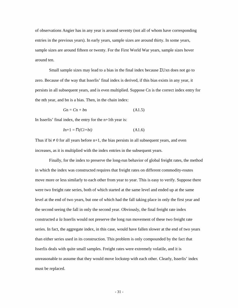
Small sample sizes may lead to a bias in the final index because ΣUxn does not go to

zero. Because of the way that Isserlis’ final index is derived, if this bias exists in any year, it

persists in all subsequent years, and is even multiplied. Suppose Cn is the correct index entry for

the nth year, and bn is a bias. Then, in the chain index:

Gn = Cn + bn (A1.5)

In Isserlis’ final index, the entry for the n+1th year is:

In+1 = Π(Ci+bi) (A1.6)

Thus if bi ≠ 0 for all years before n+1, the bias persists in all subsequent years, and even

increases, as it is multiplied with the index entries in the subsequent years.

Finally, for the index to preserve the long-run behavior of global freight rates, the method

in which the index was constructed requires that freight rates on different commodity-routes

move more or less similarly to each other from year to year. This is easy to verify. Suppose there

were two freight rate series, both of which started at the same level and ended up at the same

level at the end of two years, but one of which had the fall taking place in only the first year and

the second seeing the fall in only the second year. Obviously, the final freight rate index

constructed a la Isserlis would not preserve the long run movement of these two freight rate

series. In fact, the aggregate index, in this case, would have fallen slower at the end of two years

than either series used in its construction. This problem is only compounded by the fact that

Isserlis deals with quite small samples. Freight rates were extremely volatile, and it is

unreasonable to assume that they would move lockstep with each other. Clearly, Isserlis’ index

must be replaced.

- 32 -

Appendix 2: Construction of the Regional and Global Freight Rate Indices

Angiers 1869-1950

The Angier dataset was broken up into smaller regional datasets based upon the location

of ports and the availability of data. Wherever possible, ports that were included in a region were

not separated from each other by more than 10% of the distance from Europe.11 We also

separated outbound from homeward routes. Consulting contemporary sources that reported

commodity stowage factors, we identified commodities with similar stowage factors for each

region.

Starting with the first year in this restricted regional dataset, we took a segment of the

dataset covering all years in which the freight rates for the same commodity-routes were quoted.

We then took the simple average of these quoted freight rates for each year, and formed an index

from these averages. We then took the year that immediately followed the last year in the first

segment, and formed a new segment covering all years which contained the same commodity-

routes. Again, we took the simple average of the freight rates quoted for each year, and formed an

index from these averages. If the first and second segments had some commodity-routes in

common, we linked them in the following manner: We first take the simple average of the freight

rates on the shared commodity-routes in the last year of the first segment in which this overlap

takes place. We mark this as A. We then take the simple average of the freight rates on the shared

commodity-routes in the first year of the second segment in which this overlap takes place. We

mark this as B. We rebase the second segment index in Bs year. We form the ratio of B to A. We

multiply all the entries in the rebased second index with this ratio. This rebased second segment is

then grafted to the first segment to form an index covering the full period.

11 For two regions out of seventeen – East Asia (comprising of the Philippines, Japan and China) and WestAfrica – data limitations forced us to violate this condition.

- 33 -

If the first and second segment have no commodity-routes in common, we form a third

segment with all years where the freight rates of exactly the same commodity-routes as the year

immediately following the last year of the second segment were quoted. We form a index for this

segment in the same manner described above. We then see if the segment shared commodity-

routes with the first segment. If so, we link the first and third index in the manner described in the

last paragraph. To link this combination index formed from the first and third segment indices

(“first-third combination index”) to the second segment index we first link the second and third

indices in the manner described in the last paragraph (to form the “second-third combination

index”). We rebase the second-third combination index in the year (call it year X) in the third

segment that was used for linking the third segment to the second segment. We then multiply all

entries in this rebased second-third combination index with the entry for year X in the first-third

combination index.

Obviously, if the first, second and third segments do not share commodity-routes, the

procedure can be repeated until segments with some overlapping commodity-routes are found. Of

course, the procedure does not guarantee that each segment with have overlapping commodity-

routes with some other segment. If this happens, we are forced to find new freight rate data that

will allow us to carry out the linking.

Note that it does not matter what year within segments is taken as the base year. The ratio

of the average of nominal freight rates at any year to the average of nominal freight rates at

another year within the segment is preserved independent of the choice of base year. We are thus

able to rebase segments at the linking years and not introduce any biases. To link across

segments, it is assumed that had Angier been consistent in his choices of commodity-routes, the

missing data would not substantially change the ratio of the average nominal freight rate in one

segment’s linking year to the average nominal freight rate for another segment’s linking year

from the ratio calculated from the incomplete data. The competitive nature of the tramp shipping

- 34 -

industry and the fact that we are including routes where only commodities with comparable

stowage factors were carried allow us to feel somewhat comfortable with this assumption.

Our global index of long distance tramp freight rates between Europe and the rest of the

world requires us to weight the different regional indices according to the importance of trade to

and from that region. We use the Board of Trade figures (Mitchell 1992) to compute the value of

trade between Britain and the different regions in the dataset, and find the percentage of total

trade to these regions to Britain being carried from individual regions. These percentages formed

the weights for the homeward routes. For outbound coal freights on various routes, the limitations

of the Angier data forced us to take the simple average of available indices of coal freights along

the routes. The outbound coal freight and the homeward freight indices were then aggregated

taking their simple average.

Linking Angiers with the Post-WW II Era

The Norwegian Shipping News (NSN) index for tramp voyage charter party freight rates

reported by Hummels (1999) is based in 1947, but has a gap between 1947 and 1952. Since our

Angiers-based global freight rate index has an entry for 1945-49, the NSN index can be easily

linked to it. To fill the gap between 1947 and 1952, the Italian freight index reported by Sturmey

(1962: p. 179) is used.

Even though the three indices used here relate to tramp shipping from different countries

and are weighted up differently, they are highly correlated. Hummels (1999: p. 27) reports a

correlation of 0.87 between British and Norwegian charters rates, and we computed a correlation

of 0.99 between the Italian and Norwegian indices.

Appendix 3: Deflated Regional Freight Rate Indices

Table A3A: Non-Atlantic Routes Deflated by the Sauerbeck Index

Table A3B: Atlantic Routes Deflated by the Sauerbeck Index

- 35 -

Table A3C: Non-Atlantic Routes Deflated by Commodity Prices in Britain

Table A3D: Atlantic Routes Deflated by Commodity Prices in Britain

Appendix 4: Productivity Growth Calculations

Wages

Nearly a century after they were compiled, Bowley’s indices of income and wages

remain standard sources for the late-19th and early-20th century Britain.12 Bowley included in his

work a wage index for British able-bodies seamen (ABS) covering the years between 1870 and

1890. The information is taken from 11 voyages started each from year from each of the major

ports in Great Britain. Harley used this index in his productivity gains calculations. For the period

between 1890 and 1913, the Board of Trade collected wage rates for various classes of seamen. It

is easy to construct an index of wage rates for seamen by taking unweighted averages (i.e., fixed

weights) of wage rates for various classes of seamen.

However, crew composition must have changed drastically in this period. Due to

economies of scale and increasing steam engine efficiency, the number of ABS, firemen and coal

trimmers would have decreased. The share of officers in the crew would thus have increased, as

the number of officers would have remained more or less fixed. Given the fact that officers were

paid more than ABS, Bowley’s index would have overstated the fall in average crew wages. It is

easy to see that taking an unweighted average of wage rates for the various classes of mariners

does precisely the same thing.

The Atlantic Canada Shipping Project (ACSP) at the Memorial University of

Newfoundland has compiled a 1% random sample of British Agreements and Accounts of Crews

between 1863 and 1913. These were official documents mandated by law and were required to be

completed whenever a crew signed onto a ship, regardless of the port. The documents included

such information as ship and voyage details, as well as rank and personal information of

- 36 -

individual crewmembers, including the wage rates agreed upon by them. Overall, we have

information on about 80,000 seamen of all ranks in this sample. Taking the simple average of

wage rates for all seamen – regardless of rank – in a particular year and forming an index from

these averages improves upon Bowley’s and Feinstein’s in two ways.

First, the index does not depend solely upon wages quoted in major British ports. True,

the crew on British vessels was mostly hired in Britain, and hiring most of the necessary crew in

one location was more efficient than stopping at a number of ports to add crewmembers and

incurring associated costs. Large ports like Liverpool and London were also centers of the

shipping labor market, but expanding the wage estimates to include non-British seamen hired in

non-British ports is a significant improvement. Second, taking a simple average of wage rates for

all seamen takes into account changing crew composition. As crew composition changes, the

number of observations for each rank relative to the total number of observations for that year in

our sample also changes. In effect, the simple average of wage rates is weighted, according to

crew composition. The wage rate index created does not have a fixed-weight bias toward the

wages for a particular rank

The ACSP sample ends in 1913. For the period between the two World Wars, we turn to

Chapman’s average earnings data collected from the Annual Yearbook of the National Maritime

Board (summary of Agreement) and the quinquennial censuses of seamen. This index is a

weighted average of monthly rates for various ranks of seamen, and controls for different sizes of

vessels. The wage rates reported do not include overtime pay.

Cost of Capital

The cost of capital in each period was calculated from the following formula:

CKt = PKt (r + d)

12 Feinstein (1972) improved on these data recently by revisiting Bowley’s sources.

- 37 -

where CKt is the cost of capital in time t; r is the interest rate; d is the rate of depreciation; PK is

the price of the ship per gross ton in that period. As has been standard in the literature, we assume

that r and d remain unchanged in this period.

A number of studies have examined ship prices in the age of steam. We use data from

Harley (1972: pp. 250-57) to estimate average ship price per ton for the period between 1871 and

1889. Pollard and Robertson use data from Fairplay magazine to trace the price of

“representative” ships in the period between 1887 and 1913. It is unclear to what degree the

Pollard-Robertson index controls for increasing vessel size, but we assume that it represents ship

prices per gross ton, with a standard engine attached, allowing for changes in engine quality. For

the interwar period, we use the Maywald index of British ship prices, also used by Feinstein

(1972: p. T137) in his construction of an index of British capital expenditure.13

Price of Coal

Ideally, we would have liked to have taken into account the price of coal at bunker

(refueling) ports on each route. However, reliable bunker coal price series are unavailable.

Instead, we construct a bunker coal price index in two steps. First, we take the sum of the freight

rate for coal shipped to the destination and the average price of British exported coal (reported by

Sauerbeck) as a initial proxy for the price of bunker coal. Second, the initial bunker coal proxy

price index is then multiplied by 1.25 to take into account port costs during refueling.

Port Charges

Urquhart published a review of charges and dues in non-British ports regularly in the

second half of the 19th century. This work was continued by Ritherdon in the first half of the 20th

century. While these publications suggest that port charges per gross registered ton may have

13 Both Pollard-Robertson and Harley note serious problems with this index, especially since it does notcontrol for the increasing complexity of navy ships whose prices Maywald used to construct the index.

- 38 -

fallen over the period, it is difficult to say by how much. Therefore port charges are ignored in

our TFP calculations.

Factor Shares

We use Harley’s (1972: p. 312) estimates of factor shares for the period between 1869

to1890. These were mined from contemporary sources. Roberts (1947: p. 297) presents the shares

of various inputs in coal-burning steamers in the early 1920s. These factor share estimates are

comparable to Harley’s for the late 19th century. Griffiths’ (1995: pp. 323-26) reports of operating

costs in 1922 and 1926 agree with this assessment. Fayle’s comparative figures for a ship voyage

from Cardiff, to Algiers, New Orleans and Rotterdam in 1913 and 1920 also suggest that it is

reasonable to use Harley’s factor share estimates for the period between 1890 and 1913 as well as

for the 1920s. These factor share estimates are presented in table following:

Factor Shares (%)Capital Costs (interest, depreciation, repairs) 40Fuel Costs (Coal) 20Labor Costs (Wages + Provisions) 10Port Charges 25Others 5

These factor shares are used as fixed weights for the entire period in the productivity calculations.

Appendix 5: Explanation of the TFP Growth Calculation

The explanation for TFP growth using quantities of factors used is derived as follows:

A* = Pi* – Pf* = Q* – Qi*

where A* is the percentage change in total factor productivity, Pi* is the percentage change in the

index of factor prices weighted by factor shares, Pf* is the percentage change in the freight index,

Q* is the percentage change in the quantity of goods carried, and Qi* is the percentage change in

the index of quantities of inputs weighted by factor shares. The percentage change in quantity of

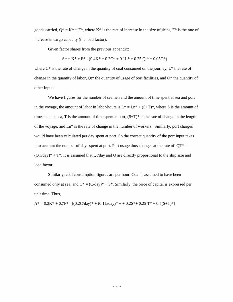
- 39 -

goods carried, Q* = K* + F*, where K* is the rate of increase in the size of ships, F* is the rate of

increase in cargo capacity (the load factor).

Given factor shares from the previous appendix:

A* = K* + F* - (0.4K* + 0.2C* + 0.1L* + 0.25 Qt* + 0.05O*)

where C* is the rate of change in the quantity of coal consumed on the journey, L* the rate of

change in the quantity of labor, Qt* the quantity of usage of port facilities, and O* the quantity of

other inputs.

We have figures for the number of seamen and the amount of time spent at sea and port

in the voyage, the amount of labor in labor-hours is L* = Ln* + (S+T)*, where S is the amount of

time spent at sea, T is the amount of time spent at port, (S+T)* is the rate of change in the length

of the voyage, and Ln* is the rate of change in the number of workers. Similarly, port charges

would have been calculated per day spent at port. So the correct quantity of the port input takes

into account the number of days spent at port. Port usage thus changes at the rate of QT* =

(QT/day)* + T*. It is assumed that Qt/day and O are directly proportional to the ship size and

load factor.

Similarly, coal consumption figures are per hour. Coal is assumed to have been

consumed only at sea, and C* = (C/day)* + S*. Similarly, the price of capital is expressed per

unit time. Thus,

A* = 0.3K* + 0.7F* - [(0.2C/day)* + (0.1L/day)* + + 0.2S*+ 0.25 T* + 0.5(S+T)*]

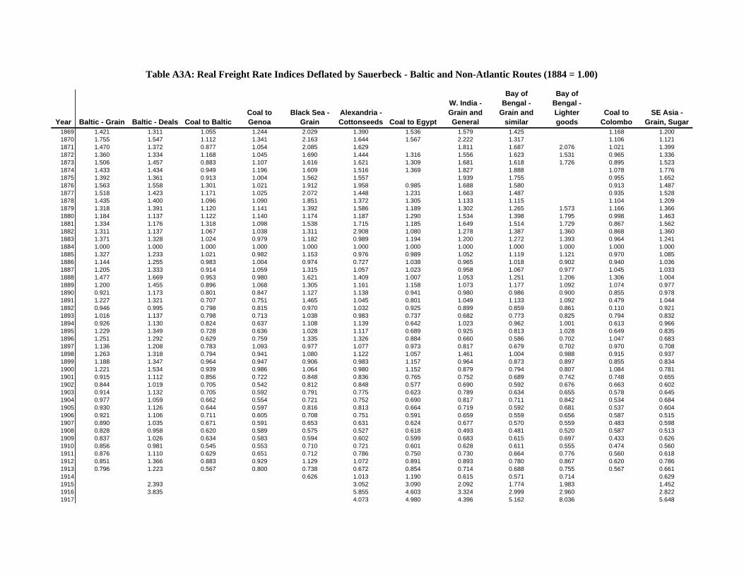
Table A3A: Real Freight Rate Indices Deflated by Sauerbeck - Baltic and Non-Atlantic Routes (1884 = 1.00)

Year Baltic - Grain Baltic - Deals Coal to BalticCoal to Genoa

Black Sea - Grain

Alexandria - Cottonseeds Coal to Egypt

W. India - Grain and General

Bay of Bengal -

Grain and similar

Bay of Bengal - Lighter goods

Coal to Colombo

SE Asia - Grain, Sugar

1869 1.421 1.311 1.055 1.244 2.029 1.390 1.536 1.579 1.425 1.168 1.2001870 1.755 1.547 1.112 1.341 2.163 1.644 1.567 2.222 1.317 1.106 1.1211871 1.470 1.372 0.877 1.054 2.085 1.629 1.811 1.687 2.076 1.021 1.3991872 1.360 1.334 1.168 1.045 1.690 1.444 1.316 1.556 1.623 1.531 0.965 1.3361873 1.506 1.457 0.883 1.107 1.616 1.621 1.309 1.681 1.618 1.726 0.895 1.5231874 1.433 1.434 0.949 1.196 1.609 1.516 1.369 1.827 1.888 1.078 1.7761875 1.392 1.361 0.913 1.004 1.562 1.557 1.939 1.755 0.955 1.6521876 1.563 1.558 1.301 1.021 1.912 1.958 0.985 1.688 1.580 0.913 1.4871877 1.518 1.423 1.171 1.025 2.072 1.448 1.231 1.663 1.487 0.935 1.5281878 1.435 1.400 1.096 1.090 1.851 1.372 1.305 1.133 1.115 1.104 1.2091879 1.318 1.391 1.120 1.141 1.392 1.586 1.189 1.302 1.265 1.573 1.166 1.3661880 1.184 1.137 1.122 1.140 1.174 1.187 1.290 1.534 1.398 1.795 0.998 1.4631881 1.334 1.176 1.318 1.098 1.538 1.715 1.185 1.649 1.514 1.729 0.867 1.5621882 1.311 1.137 1.067 1.038 1.311 2.908 1.080 1.278 1.387 1.360 0.868 1.3601883 1.371 1.328 1.024 0.979 1.182 0.989 1.194 1.200 1.272 1.393 0.964 1.2411884 1.000 1.000 1.000 1.000 1.000 1.000 1.000 1.000 1.000 1.000 1.000 1.0001885 1.327 1.233 1.021 0.982 1.153 0.976 0.989 1.052 1.119 1.121 0.970 1.0851886 1.144 1.255 0.983 1.004 0.974 0.727 1.038 0.965 1.018 0.902 0.940 1.0361887 1.205 1.333 0.914 1.059 1.315 1.057 1.023 0.958 1.067 0.977 1.045 1.0331888 1.477 1.669 0.953 0.980 1.621 1.409 1.007 1.053 1.251 1.206 1.306 1.0041889 1.200 1.455 0.896 1.068 1.305 1.161 1.158 1.073 1.177 1.092 1.074 0.9771890 0.921 1.173 0.801 0.847 1.127 1.138 0.941 0.980 0.986 0.900 0.855 0.9781891 1.227 1.321 0.707 0.751 1.465 1.045 0.801 1.049 1.133 1.092 0.479 1.0441892 0.946 0.995 0.798 0.815 0.970 1.032 0.925 0.899 0.859 0.861 0.110 0.9211893 1.016 1.137 0.798 0.713 1.038 0.983 0.737 0.682 0.773 0.825 0.794 0.8321894 0.926 1.130 0.824 0.637 1.108 1.139 0.642 1.023 0.962 1.001 0.613 0.9661895 1.229 1.349 0.728 0.636 1.028 1.117 0.689 0.925 0.813 1.028 0.649 0.8351896 1.251 1.292 0.629 0.759 1.335 1.326 0.884 0.660 0.586 0.702 1.047 0.6831897 1.136 1.208 0.783 1.093 0.977 1.077 0.973 0.817 0.679 0.702 0.970 0.7081898 1.263 1.318 0.794 0.941 1.080 1.122 1.057 1.461 1.004 0.988 0.915 0.9371899 1.188 1.347 0.964 0.947 0.906 0.983 1.157 0.964 0.873 0.897 0.855 0.8341900 1.221 1.534 0.939 0.986 1.064 0.980 1.152 0.879 0.794 0.807 1.084 0.7811901 0.915 1.112 0.856 0.722 0.848 0.836 0.765 0.752 0.689 0.742 0.748 0.6551902 0.844 1.019 0.705 0.542 0.812 0.848 0.577 0.690 0.592 0.676 0.663 0.6021903 0.914 1.132 0.705 0.592 0.791 0.775 0.623 0.789 0.634 0.655 0.578 0.6451904 0.977 1.059 0.662 0.554 0.721 0.752 0.690 0.817 0.711 0.842 0.534 0.6841905 0.930 1.126 0.644 0.597 0.816 0.813 0.664 0.719 0.592 0.681 0.537 0.6041906 0.921 1.106 0.711 0.605 0.708 0.751 0.591 0.659 0.559 0.656 0.587 0.5151907 0.890 1.035 0.671 0.591 0.653 0.631 0.624 0.677 0.570 0.559 0.483 0.5981908 0.828 0.958 0.620 0.589 0.575 0.527 0.618 0.493 0.481 0.520 0.587 0.5131909 0.837 1.026 0.634 0.583 0.594 0.602 0.599 0.683 0.615 0.697 0.433 0.6261910 0.856 0.981 0.545 0.553 0.710 0.721 0.601 0.628 0.611 0.555 0.474 0.5601911 0.876 1.110 0.629 0.651 0.712 0.786 0.750 0.730 0.664 0.776 0.560 0.6181912 0.851 1.366 0.883 0.929 1.129 1.072 0.891 0.893 0.780 0.867 0.620 0.7861913 0.796 1.223 0.567 0.800 0.738 0.672 0.854 0.714 0.688 0.755 0.567 0.6611914 0.626 1.013 1.190 0.615 0.571 0.714 0.6291915 2.393 3.052 3.090 2.092 1.774 1.983 1.4521916 3.835 5.855 4.603 3.324 2.999 2.960 2.8221917 4.073 4.980 4.396 5.162 8.036 5.648

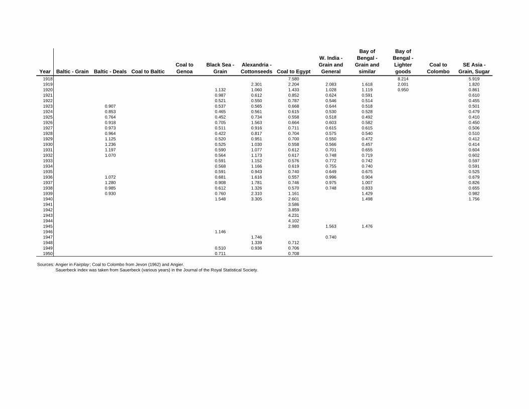
Year Baltic - Grain Baltic - Deals Coal to BalticCoal to Genoa

Black Sea - Grain

Alexandria - Cottonseeds Coal to Egypt

W. India - Grain and General

Bay of Bengal -

Grain and similar

Bay of Bengal - Lighter goods

Coal to Colombo

SE Asia - Grain, Sugar

1918 7.580 8.214 5.9191919 2.301 2.204 2.083 1.618 2.001 1.8201920 1.132 1.060 1.433 1.028 1.119 0.950 0.8611921 0.987 0.612 0.852 0.624 0.591 0.6101922 0.521 0.550 0.787 0.546 0.514 0.4551923 0.907 0.537 0.565 0.668 0.644 0.518 0.5011924 0.853 0.465 0.561 0.615 0.530 0.528 0.4791925 0.764 0.452 0.734 0.558 0.518 0.492 0.4101926 0.918 0.705 1.563 0.664 0.603 0.582 0.4501927 0.973 0.511 0.916 0.711 0.615 0.615 0.5061928 0.964 0.422 0.817 0.704 0.575 0.540 0.5101929 1.125 0.520 0.951 0.700 0.550 0.472 0.4121930 1.236 0.525 1.030 0.558 0.566 0.457 0.4141931 1.197 0.590 1.077 0.612 0.701 0.655 0.6041932 1.070 0.564 1.173 0.617 0.748 0.719 0.6021933 0.591 1.152 0.576 0.772 0.742 0.5971934 0.568 1.166 0.619 0.755 0.740 0.5911935 0.591 0.943 0.740 0.649 0.675 0.5251936 1.072 0.681 1.616 0.557 0.996 0.904 0.6791937 1.280 0.908 1.781 0.746 0.975 1.007 0.8261938 0.985 0.612 1.326 0.570 0.748 0.833 0.6551939 0.930 0.760 2.310 1.161 1.429 0.9821940 1.548 3.305 2.601 1.498 1.7561941 3.5861942 3.8591943 4.2311944 4.1021945 2.980 1.563 1.4761946 1.1461947 1.746 0.7401948 1.339 0.7121949 0.510 0.936 0.7061950 0.711 0.708

Sources: Angier in Fairplay ; Coal to Colombo from Jevon (1962) and Angier. Sauerbeck index was taken from Sauerbeck (various years) in the Journal of the Royal Statistical Society.

Table A3B: Real Freight Rate Indices Deflated by Sauerbeck - Atlantic Routes (1884 = 1.00)

Year

E. Latin America -

Grain

W. Latin America -

NitrateCoal to E.

Latin AmericaCoal to W.

Latin America

E. North America -

Timber

E. North America -

Grain

W. North America -

Grain

N. America Gulf Coast -

Cotton

N. America Gulf Coast -

Timber

N. America Gulf Coast -

Grain

Western Mediterranean

- Ore1869 0.875 0.792 1.073 1.668 1.129 1.374 1.398 0.9751870 0.749 0.943 0.965 1.136 1.131 1.314 1.255 0.9681871 0.890 1.087 0.976 1.137 1.127 1.359 1.059 0.937 1.3281872 0.857 1.036 0.979 1.180 1.091 3.134 1.459 0.9251873 0.894 1.108 1.084 1.082 1.399 1.421 1.619 1.191 1.6861874 0.915 1.236 1.008 1.179 1.539 1.393 1.569 1.2191875 0.982 1.110 0.882 0.728 1.554 1.1631876 0.920 1.037 0.855 0.830 1.347 1.342 1.4511877 0.862 0.984 0.838 0.808 1.367 0.969 1.3231878 0.854 0.830 0.904 0.797 1.475 1.112 1.1331879 0.871 0.918 0.976 0.869 1.355 1.341 1.146 1.0341880 0.933 0.958 0.933 0.848 1.211 1.493 0.989 1.2111881 0.989 1.109 0.921 0.810 1.010 2.034 0.9461882 1.000 1.253 0.985 0.863 1.181 1.465 1.074 1.2311883 0.905 0.953 1.013 0.914 1.197 1.120 1.107 1.000 1.1361884 1.000 1.000 1.000 1.000 1.000 1.000 1.000 1.000 1.000 1.000 1.0001885 0.986 0.787 0.933 1.046 1.021 0.984 1.013 1.122 1.048 1.0231886 0.914 0.768 0.892 1.049 0.973 1.168 0.961 0.971 1.170 1.015 1.0441887 1.130 0.892 0.987 1.100 0.973 0.969 0.877 0.997 0.961 0.927 1.2921888 1.078 0.925 1.223 1.616 1.279 1.256 0.947 1.177 1.126 1.163 1.5261889 1.218 0.984 1.508 1.486 1.407 1.425 0.995 1.184 1.496 1.247 1.3571890 1.343 1.057 1.122 1.400 0.987 1.242 1.161 0.875 1.242 1.068 1.3551891 1.628 0.872 0.856 0.629 0.926 1.222 1.105 0.931 1.068 1.003 1.2881892 1.395 0.446 0.818 0.695 1.002 1.248 0.819 0.824 1.145 1.030 1.1341893 1.226 0.816 0.783 0.883 0.962 0.992 0.799 0.927 1.159 0.852 1.2251894 1.390 0.821 0.662 0.749 1.006 1.188 0.895 1.036 1.234 1.016 1.4781895 1.221 0.707 0.639 0.742 1.038 1.158 1.067 0.902 1.254 1.175 1.3971896 1.103 0.671 0.814 0.908 1.070 1.422 0.868 0.917 1.274 1.247 1.6831897 1.014 0.907 0.840 0.894 1.022 1.303 1.017 0.869 1.207 1.180 1.5021898 1.258 0.990 0.869 0.995 1.141 1.380 0.962 0.970 1.470 1.426 1.6361899 1.507 0.964 0.614 0.937 1.046 1.116 1.132 0.865 1.265 1.228 1.3891900 1.168 1.020 0.798 0.813 1.191 1.224 1.218 0.881 1.228 1.365 1.5641901 0.982 0.851 0.631 0.858 0.962 0.835 1.246 0.658 1.071 0.977 1.2391902 0.904 0.648 0.555 0.536 0.836 0.673 0.902 0.566 0.919 0.879 1.3221903 1.037 0.492 0.469 0.810 0.906 0.760 0.603 0.597 0.926 0.839 1.2711904 1.108 0.655 0.413 0.558 0.797 0.835 0.718 0.541 0.920 0.791 1.1641905 0.841 0.609 0.488 0.543 0.789 0.854 0.763 0.585 0.855 0.846 1.2591906 0.743 0.536 0.581 0.554 0.692 0.770 0.769 0.540 0.802 0.702 1.1781907 0.756 0.435 0.551 0.966 0.762 0.655 0.976 0.525 0.779 0.709 1.0751908 0.749 0.482 0.477 0.817 0.596 0.853 0.507 0.810 0.714 1.0341909 0.640 0.541 0.474 0.713 0.587 0.828 0.562 0.750 0.628 1.0381910 0.608 0.540 0.649 0.699 0.529 0.819 0.549 0.750 0.662 1.0821911 0.642 0.556 0.736 0.905 0.705 0.939 0.761 0.648 1.1141912 1.112 0.677 0.803 1.016 0.944 1.130 1.070 0.983 1.2771913 0.944 0.702 0.677 1.031 0.804 1.130 0.902 0.826 1.1001914 1.174 0.639 0.607 1.293 0.980 0.852 0.767 1.0171915 2.469 1.330 1.024 1.827 2.737 1.788 1.798 1.595 0.602 2.1451916 3.492 2.044 1.399 3.313 3.267 2.477 2.834 0.580 2.3871917 7.096 2.006 2.231 4.841 3.672

Year

E. Latin America -

Grain

W. Latin America -

NitrateCoal to E.

Latin AmericaCoal to W.

Latin America

E. North America -

Timber

E. North America -

Grain

W. North America -

Grain

N. America Gulf Coast -

Cotton

N. America Gulf Coast -

Timber

N. America Gulf Coast -

Grain

Western Mediterranean

- Ore1918 4.567 2.539 0.920 2.6991919 3.831 2.199 0.683 2.249 1.506 1.374 3.442 1.7411920 1.805 0.757 0.230 1.509 1.057 1.182 0.899 0.944 1.8651921 0.905 0.731 0.337 1.235 0.520 0.987 0.963 0.765 1.0841922 0.848 0.523 0.353 0.816 0.613 0.655 0.786 0.532 1.0571923 0.696 0.521 0.453 0.813 0.550 0.626 0.776 0.479 1.0671924 0.761 0.408 0.294 0.770 0.570 0.580 0.732 0.487 0.9421925 0.582 0.384 0.291 0.716 0.475 0.578 0.715 0.428 0.8981926 1.037 0.422 0.378 0.756 0.909 0.640 0.612 0.482 1.2041927 0.897 0.532 0.348 0.897 0.536 0.647 0.830 0.495 0.9261928 0.776 0.442 0.249 0.803 0.631 0.599 0.719 0.453 0.9351929 0.680 0.447 0.250 1.011 0.505 0.563 0.779 0.437 1.0531930 0.670 0.477 0.307 1.064 0.422 0.490 0.857 0.375 1.0211931 0.907 0.567 0.347 0.987 0.500 0.635 0.872 0.436 1.0781932 0.860 0.572 0.349 0.988 0.551 0.602 0.651 1.1241933 0.815 0.557 0.380 0.964 0.483 0.563 0.644 1.2191934 0.789 0.467 0.440 0.976 0.439 0.540 0.605 1.1751935 0.785 0.471 0.450 0.953 0.511 0.500 0.610 1.2231936 1.048 0.422 0.586 1.084 0.567 0.645 0.689 1.6551937 1.225 1.142 1.370 0.937 0.827 0.811 2.1941938 1.114 1.453 1.103 0.807 0.672 0.634 1.7091939 1.626 1.741 1.667 1.993 0.954 1.350 4.4661940 3.280 1.531 3.575 2.484 1.651 2.335 7.8191941 1.3831942 1.117194319441945 0.527 1.767 1.515 1.605 4.5651946 0.729 1.416 1.166 1.425 3.9081947 0.877 0.606 1.195 0.962 1.250 2.9461948 0.682 0.879 0.776 0.971 2.3251949 0.588 0.785 0.564 1.152 1.9321950 0.364 0.773 0.663 0.768 1.855

Sources: Angier in Fairplay ; W. Latin America Nitrate before 1890 from Stemmer (1989); E. Latin America Grain before 1880 from Harley (1989); Coal to Latin America from Jevons (1962) and Angier. Sauerbeck index was taken from Sauerbeck (various years) in the Journal of the Royal Statistical Society.

Table A3C: Real Commodity Deflated Freight Rate Indices - Baltic and Non-Atlantic Routes (1884 = 1.00)

Year Baltic - Grain Baltic - Deals Coal to BalticCoal to Genoa

Black Sea - Grain

Alexandria - Cottonseeds Coal to Egypt

W. India - Grain and General

Bay of Bengal -Grain and

similar

Bay of Bengal -Lighter goods

(Jute)Coal to

ColomboSE Asia -

Grain, Sugar1869 1.384 1.516 1.307 1.540 1.926 0.720 1.901 1.499 1.475 1.446 1.0421870 1.804 1.719 1.346 1.624 2.070 1.001 1.897 2.126 1.336 1.339 0.9531871 1.358 1.794 1.087 1.307 1.716 1.443 1.491 1.721 1.559 1.266 1.1981872 1.412 1.782 0.975 0.872 1.505 1.079 1.099 1.386 1.771 1.435 0.806 1.2601873 1.505 1.566 0.569 0.713 1.423 1.494 0.843 1.481 1.892 1.875 0.577 1.5541874 1.280 1.353 0.683 0.861 1.375 1.499 0.985 1.561 1.930 0.776 1.6811875 1.304 1.405 0.802 0.882 1.550 1.541 1.923 2.050 0.839 1.6571876 1.500 1.591 1.375 1.080 1.837 2.131 1.041 1.622 1.674 0.965 1.3911877 1.301 1.389 1.316 1.152 1.603 1.353 1.384 1.286 1.403 1.052 1.2461878 1.308 1.470 1.228 1.221 1.623 1.248 1.462 0.993 0.975 1.237 1.0091879 1.247 1.622 1.293 1.317 1.234 1.361 1.372 1.154 1.103 1.403 1.346 1.1361880 1.146 1.161 1.343 1.365 1.090 1.027 1.545 1.424 1.362 1.491 1.195 1.2781881 1.269 1.207 1.523 1.269 1.350 1.722 1.369 1.447 1.554 1.407 1.002 1.3401882 1.235 1.109 1.196 1.163 1.143 2.928 1.210 1.115 1.581 1.350 0.972 1.2371883 1.219 1.370 1.096 1.047 1.091 1.083 1.277 1.108 1.299 1.373 1.031 1.0891884 1.000 1.000 1.000 1.000 1.000 1.000 1.000 1.000 1.000 1.000 1.000 1.0001885 1.283 1.179 0.992 0.954 1.172 0.846 0.961 1.069 1.147 1.180 0.943 1.0621886 1.136 1.205 0.970 0.990 1.006 0.721 1.024 0.996 1.064 0.951 0.927 1.1111887 1.244 1.291 0.903 1.046 1.277 1.033 1.010 0.930 1.059 0.952 1.032 1.0631888 1.563 1.588 0.958 0.985 1.653 1.303 1.013 1.074 1.232 1.119 1.314 0.9951889 1.314 1.279 0.763 0.910 1.464 1.038 0.986 1.204 1.165 0.920 0.915 0.9001890 0.952 1.098 0.552 0.584 1.179 1.065 0.648 1.025 0.976 0.858 0.589 1.0081891 1.134 1.323 0.506 0.537 1.322 1.185 0.573 0.946 1.027 1.061 0.343 1.0191892 0.916 0.920 0.594 0.606 1.011 1.199 0.689 0.938 0.760 0.685 0.082 0.8511893 1.080 1.076 0.657 0.587 1.244 0.961 0.607 0.817 0.850 0.758 0.654 0.8221894 1.024 0.969 0.599 0.462 1.420 1.402 0.466 1.311 1.038 0.887 0.445 1.0251895 1.456 1.194 0.586 0.511 1.283 1.292 0.554 1.155 0.916 1.019 0.522 0.9621896 1.360 1.074 0.525 0.634 1.447 1.342 0.737 0.715 0.579 0.615 0.874 0.7151897 1.091 0.955 0.654 0.913 0.933 1.118 0.813 0.780 0.623 0.695 0.811 0.7581898 1.130 1.075 0.620 0.734 0.944 1.472 0.825 1.277 0.895 1.011 0.714 0.9721899 1.348 1.118 0.739 0.726 1.113 1.245 0.887 1.185 0.826 0.857 0.656 0.9031900 1.485 1.244 0.514 0.540 1.392 0.910 0.631 1.150 0.820 0.755 0.594 0.9151901 1.004 0.895 0.522 0.441 1.030 0.864 0.467 0.912 0.730 0.715 0.457 0.8091902 0.850 0.825 0.478 0.368 0.925 0.812 0.391 0.786 0.661 0.669 0.449 0.8381903 1.027 0.865 0.502 0.422 0.946 0.664 0.444 0.944 0.602 0.588 0.412 0.7711904 1.112 0.869 0.503 0.421 0.826 0.539 0.524 0.936 0.754 0.739 0.406 0.8211905 1.032 0.950 0.530 0.491 0.918 0.721 0.546 0.809 0.630 0.465 0.442 0.7021906 1.100 0.937 0.614 0.522 0.905 0.623 0.510 0.843 0.598 0.381 0.507 0.6871907 1.047 0.878 0.514 0.453 0.800 0.588 0.478 0.830 0.556 0.378 0.370 0.7411908 0.883 0.789 0.428 0.406 0.608 0.457 0.427 0.522 0.461 0.430 0.405 0.5911909 0.828 0.852 0.508 0.467 0.559 0.474 0.480 0.643 0.649 0.705 0.347 0.7521910 1.007 0.812 0.443 0.450 0.820 0.485 0.488 0.726 0.662 0.521 0.386 0.6741911 1.013 0.941 0.538 0.556 0.843 0.542 0.641 0.865 0.655 0.544 0.479 0.6971912 0.933 1.168 0.721 0.758 1.293 0.908 0.727 1.022 0.661 0.622 0.506 0.8431913 0.970 0.996 0.421 0.594 0.924 0.519 0.635 0.895 0.721 0.429 0.421 0.8741914 0.462 0.976 0.903 0.454 0.537 0.397 0.7201915 1.647 3.874 2.387 1.801 1.448 1.787 1.4631916 2.117 5.870 3.093 2.789 2.434 2.297 2.7111917 2.765 3.909 4.940 3.597 6.323 5.019

Year Baltic - Grain Baltic - Deals Coal to BalticCoal to Genoa

Black Sea - Grain

Alexandria - Cottonseeds Coal to Egypt

W. India - Grain and General

Bay of Bengal -Grain and

similar

Bay of Bengal -Lighter goods

(Jute)Coal to

ColomboSE Asia -

Grain, Sugar1918 5.783 7.010 5.4671919 1.654 1.193 2.750 1.293 1.451 1.6741920 2.769 1.002 0.547 2.517 0.673 0.940 0.5811921 1.692 0.839 0.460 1.069 0.498 0.6751922 0.649 0.465 0.520 0.680 0.456 0.5531923 0.539 0.621 0.377 0.418 0.745 0.453 0.5071924 0.585 0.613 0.365 0.445 0.698 0.440 0.5111925 0.510 0.551 0.468 0.460 0.631 0.420 0.5241926 0.653 0.781 1.313 0.549 0.668 0.454 0.5271927 0.661 0.582 0.693 0.590 0.701 0.471 0.5641928 6.215 0.528 0.581 0.653 0.718 0.431 0.6101929 0.721 0.659 0.727 0.605 0.698 0.381 0.5231930 0.706 0.693 1.005 0.395 0.748 0.342 0.5101931 0.722 0.956 1.005 0.388 1.136 0.566 0.8081932 0.689 0.845 1.001 0.370 1.121 0.600 0.8011933 0.958 1.040 0.346 1.253 0.762 0.9461934 1.082 1.030 0.385 1.438 0.797 1.0041935 1.048 0.756 0.465 1.151 0.646 0.8131936 0.722 0.911 1.434 0.352 1.333 0.889 1.0841937 0.761 1.080 1.948 0.485 1.159 0.988 1.2731938 0.566 0.890 1.678 0.293 1.089 0.712 0.9121939 0.491 1.558 2.539 0.628 1.217 1.3011940 2.165 3.492 1.491 1.251 2.3831941 1.9221942 2.0301943 2.1571944 2.0321945 1.472 1.930 0.8921946 1.5661947 1.272 1.1091948 1.010 0.3051949 0.656 0.645 0.3231950 0.972 0.379

Sources: Angier in Fairplay ; Coal to Colombo from Jevon (1962) and Angier.Note: All UK commodity prices are taken from Sauerbeck (various years) from the Journal of the Royal Statistical Society. Alexandria - Cottonseeds has been deflated by Cotton (Fair Dhollerah) prices for data availability. Baltic - Grain has been deflated by average of oat and wheat prices. All other routes carrying grain are deflated by wheat prices.

Table A3D: Real Freight Rate Indices Deflated by Commodity Prices - Atlantic Routes (1884 = 1.00)

Year

E. Latin America -

Grain

W. Latin America -

NitrateCoal to E.

Latin AmericaCoal to W.

Latin America

E. North America -

Timber

E. North America -

Grain

W. North America -

Grain

N. America Gulf Coast -

Cotton

N. America Gulf Coast -

Timber

N. America Gulf Coast -

Grain

Western Mediterranean

- Ore1869 0.863 0.613 1.328 2.066 1.305 1.355 1.378 1.1271870 0.744 0.692 1.169 1.376 1.257 1.305 1.247 1.0761871 0.761 0.831 1.210 1.409 1.474 1.162 0.905 1.225 1.1671872 0.756 0.875 0.818 0.985 1.458 2.767 1.288 1.2361873 0.752 0.984 0.698 0.696 1.503 1.196 1.363 1.280 1.0011874 0.783 1.278 0.725 0.849 1.453 1.192 1.343 1.1501875 0.940 1.082 0.776 0.640 1.489 1.1141876 0.872 1.065 0.904 0.877 1.277 1.273 1.2761877 0.706 0.821 0.942 0.909 1.120 0.793 1.2361878 0.743 0.600 1.013 0.893 1.283 0.968 1.2661879 0.723 0.633 1.126 1.003 1.126 1.114 1.187 1.0041880 0.773 0.677 1.118 1.016 1.002 1.237 0.987 1.0611881 0.776 0.810 1.064 0.936 0.793 1.597 0.9841882 0.830 0.991 1.104 0.967 0.980 1.217 1.073 1.1131883 0.792 0.867 1.083 0.978 1.236 0.981 0.970 1.124 1.0901884 1.000 1.000 1.000 1.000 1.000 1.000 1.000 1.000 1.000 1.000 1.0001885 0.965 0.667 0.906 1.016 0.977 0.963 0.992 1.073 1.026 1.0061886 0.858 0.655 0.881 1.035 0.934 1.096 0.901 1.020 1.123 0.953 1.0381887 1.077 0.789 0.975 1.087 0.943 0.923 0.835 0.962 0.931 0.883 1.2661888 0.971 0.800 1.230 1.624 1.217 1.131 0.853 1.155 1.072 1.047 1.4601889 1.192 0.921 1.285 1.265 1.236 1.395 0.974 1.119 1.314 1.220 1.0421890 1.296 1.106 0.773 0.964 0.924 1.198 1.120 0.819 1.163 1.030 1.0201891 1.394 0.886 0.612 0.449 0.928 1.046 0.947 1.115 1.070 0.859 1.0981892 1.368 0.429 0.609 0.517 0.926 1.224 0.803 1.044 1.059 1.011 0.9351893 1.443 0.741 0.644 0.727 0.910 1.167 0.941 1.064 1.097 1.004 1.1111894 1.776 0.692 0.480 0.544 0.863 1.518 1.144 1.338 1.059 1.298 1.2751895 1.415 0.658 0.514 0.596 0.918 1.343 1.237 1.138 1.109 1.362 0.7341896 1.106 0.633 0.679 0.758 0.889 1.427 0.870 1.007 1.059 1.251 1.3711897 0.869 0.898 0.702 0.747 0.808 1.117 0.871 1.078 0.954 1.011 1.1841898 1.037 1.012 0.678 0.776 0.930 1.138 0.793 1.464 1.199 1.176 1.2711899 1.626 1.045 0.471 0.718 0.869 1.205 1.222 1.288 1.050 1.325 0.8691900 1.340 1.196 0.437 0.445 0.966 1.404 1.397 0.954 0.996 1.566 0.8791901 1.090 0.818 0.385 0.523 0.775 0.927 1.383 0.756 0.863 1.084 0.8891902 0.974 0.566 0.376 0.364 0.677 0.725 0.971 0.629 0.744 0.947 0.9931903 1.099 0.430 0.334 0.577 0.693 0.805 0.639 0.533 0.708 0.889 0.9361904 1.102 0.553 0.313 0.424 0.654 0.831 0.714 0.448 0.755 0.786 0.8861905 0.847 0.492 0.402 0.447 0.666 0.860 0.769 0.645 0.722 0.852 0.9291906 0.847 0.458 0.501 0.479 0.586 0.878 0.877 0.552 0.680 0.801 0.8431907 0.808 0.386 0.422 0.740 0.646 0.700 1.043 0.505 0.661 0.758 0.7721908 0.694 0.414 0.329 0.564 0.552 0.790 0.505 0.667 0.661 0.7451909 0.550 0.488 0.379 0.572 0.504 0.712 0.519 0.623 0.540 0.7971910 0.626 0.540 0.527 0.568 0.544 0.843 0.423 0.620 0.681 0.8751911 0.705 0.556 0.629 0.774 0.775 1.033 0.646 0.713 0.9421912 1.195 0.638 0.655 0.829 1.014 1.214 0.915 1.056 0.9901913 1.058 0.647 0.504 0.766 0.901 1.267 0.735 0.926 0.8111914 1.195 0.623 0.461 1.317 0.998 0.678 0.781 0.8301915 2.130 1.411 0.791 1.258 2.361 1.542 2.592 1.098 0.519 1.4761916 3.370 1.936 0.940 1.829 3.153 2.391 1.564 0.560 1.5851917 7.159 1.749 1.751 4.885 3.141

Year

E. Latin America -

Grain

W. Latin America -

NitrateCoal to E.

Latin AmericaCoal to W.

Latin America

E. North America -

Timber

E. North America -

Grain

W. North America -

Grain

N. America Gulf Coast -

Cotton

N. America Gulf Coast -

Timber

N. America Gulf Coast -

Grain

Western Mediterranean

- Ore1918 5.345 2.224 0.702 2.4831919 5.044 2.261 0.370 1.198 1.983 0.732 4.532 1.2431920 2.349 0.954 0.088 0.870 1.375 1.538 0.518 1.228 1.1071921 0.910 0.742 0.182 0.734 0.523 0.992 0.572 0.769 0.5891922 1.008 0.595 0.233 0.548 0.728 0.778 0.529 0.632 0.8091923 0.913 0.623 0.284 0.483 0.721 0.820 0.460 0.628 0.7791924 0.878 0.518 0.213 0.528 0.657 0.669 0.502 0.562 0.7031925 0.609 0.486 0.240 0.478 0.497 0.604 0.478 0.448 0.6911926 1.069 0.500 0.313 0.538 0.937 0.660 0.435 0.496 0.8871927 0.896 0.639 0.288 0.610 0.535 0.647 0.564 0.494 0.6711928 0.874 0.598 0.231 5.179 0.710 0.674 4.639 0.510 0.7541929 0.728 0.622 0.216 0.648 0.541 0.603 0.499 0.468 0.8311930 0.845 0.584 0.217 0.608 0.532 0.618 0.490 0.473 0.6661931 1.442 0.644 0.220 0.595 0.795 1.010 0.526 0.693 0.5961932 1.207 0.683 0.209 0.636 0.774 0.845 0.913 0.6061933 1.210 0.659 0.228 0.609 0.717 0.837 0.957 0.6691934 1.111 0.612 0.274 0.609 0.618 0.760 0.851 0.6801935 1.019 0.647 0.283 0.661 0.664 0.650 0.791 0.7181936 1.262 0.594 0.370 0.730 0.683 0.776 0.829 0.9611937 1.205 0.743 0.814 0.923 0.814 0.798 1.2171938 1.226 0.747 0.635 0.888 0.739 0.697 0.7801939 2.435 0.943 0.880 2.984 1.428 2.021 2.2771940 6.019 0.877 1.625 4.559 3.030 4.285 4.7021941 0.7411942 0.587194319441945 0.260 2.048 1.756 1.861 2.7831946 0.337 1.915 1.577 1.927 2.4861947 1.404 0.357 1.914 1.541 2.003 2.2261948 1.118 1.496 1.321 1.652 1.9131949 0.978 1.168 0.840 1.715 1.7781950 0.675 1.114 0.955 1.107 2.017

Sources: Angier in Fairplay ; W. Latin America Nitrate before 1890 from Stemmer (1989); E. Latin America Grain before 1880 from Harley (1989); Coal to Latin America from Jevons (1962) and Angier.Note: All UK commodity prices are taken from Sauerbeck (various years) from the Journal of the Royal Statistical Society. Mediterranean Ore route has been deflated by iron bar prices in UK for lack of data.

- 40 -

References

Angier, E. A. V. (1920), Fifty Year Freights. London: Fairplay.

Angier, E. A. V. (1921-1951), “Angier’s Steam Shipping Report.” In Fairplay, January

issues. London: Fairplay.

Bairoch, P. (1989), “European Trade Policy, 1815-1914.” In P. Mathias and S. Pollard

(eds.), The Cambridge Economic History of Europe vol. III. Cambridge:

Cambridge University Press.

Cage, R. A. (1997), A Tramp Shipping Dynasty - Burrell and Sons of Glasgow, 1850-

1939. Westport, Conn.: Greenwood Press.

Coatsworth, J. H. and J. G. Williamson (2002), “The Roots of Latin American

Protectionism: Looking Before the Great Depression.” NBER Working Paper

8999, National Bureau of Economic Research, Cambridge, Mass. (June).

Findlay, R. and K. H. O’Rourke (2002), “Commodity Market Integration, 1500-2000.” In

M. D. Bordo, A. M. Taylor and J. G. Williamson (eds.), Globalization in

Historical Perspective. Chicago: University of Chicago Press.

Fischer, L. R. (1989), “Around the Rim: Seamen’s Wages in North Sea Ports, 1863-

1900.” In The Baltic as Trade Route: Timber Trade in the Baltic Area –

Competition between Steam and Sails. Porvoo: Uusimaa Oy.

Fischer, L. R. and H. W. Nordvik (1986), “Maritime Transport and the Interaction of the

North Atlantic Economy, 1850-1914.” In W. Fischer et al. (eds.), The Emergence

of a World Economy 1500-1914. Wiesbaden.

Fischer, L. R. and H. W. Nordvik (1987), “Myth and Reality in Baltic Shipping: the

Wood Trade to Britain, 1863-1908.” Scandinavian Journal of History 12, 99-116.

- 41 -

Griffiths, D. (1995), “British Shipping and the Diesel Engine: The Early Years.” The

Mariner’s Mirror 81(3), 313-331.

Harley, C. K. (1972), Shipping and Shipbuilding in the Late Nineteenth Century. Harvard

University Ph.D. thesis, Cambridge, Mass.

Harley, C. K. (1980), “Transportation, the World Wheat Trade, and the Kuznets Cycle,

1850-1913.” Explorations in Economic History 17, 218-250.

Harley, C. K. (1985), “Aspects of the Economics of Shipping, 1850-1913.” In L. R.

Fischer and G. E. Panting (eds.), Change and Adaptation in Maritime History:

The North Atlantic Fleets in the Nineteenth Century. St. John’s, Newfoundland:

Memorial University of Newfoundland.

Harley, C. K. (1988), “Ocean Freight Rates and Productivity, 1740-1913: The Primacy of

Mechanical Invention Reaffirmed.” Journal of Economic History 48, 851-876.

Harley, C. K. (1989), “Coal Exports and British Shipping, 1850-1913.” Explorations in

Economic History 26: 311-338.

Harley, C. K. (1990), “North Atlantic Shipping in the Late Nineteenth Century Freight

Rates and the Interrelationship of Cargoes.” In L. R. Fischer and H. W. Nordvik

(eds.), Shipping and Trade, 1750-1950: Essays in International Maritime

Economic History. Pontefract, England: Lofthouse.

Henning, G. R. and K. Trace (1975), “Britain and the Motorship: A Case of Delayed

Adoption of New Technology?” Journal of Economic History 35, 353-385.

Hughes, C. H. (1917), Handbook of Ship Calculations. New York: D. Appleton and

Company.

- 42 -

Hummels, D. (1999), “Have International Transportation Costs Declined?” Mimeo.,

University of Chicago (November).

Imlah, J. A. H. (1958), Economic Elements in Pax Britannica: Studies in British Foreign

Trade in the Nineteenth Century. Cambridge, Mass.: Harvard University Press.

Isserliss, L. (1938), “Tramp Shipping Cargoes and Freights.” Journal of Royal Statistical

Society 101 (Part 1), 304-417.

Maddison, A. (1995), Monitoring the World Economy, 1820-1992. Paris: OECD

Development Centre Studies.

Mitchell, B. R. (1992), Abstract of British Historical Statistics. Cambridge: Cambridge

University Press.

North, D. C. (1958), “Ocean Freight Rates and Economic Development 1750-1913.”

Journal of Economic History 18: 537-55.

North, D. C. (1965), “The Role of Transportation in the Economic Development of North

America.” In Les Grandes voies maritimes dans le monde, XV-XIX siecles. Paris.

North D. C. (1968), “Sources of Productivity Change in Ocean Shipping, 1600-1850.”

Journal of Political Economy 76, 953-970.

O’Rourke, K. H. and J. G. Williamson (1999), Globalization and History: The Evolution

of a Nineteenth Century Atlantic Economy. Cambridge, Mass.: MIT Press.

Pollard, S and Robertson, P. (1979), The British Shipbuilding Industry 1870-1914.

Cambridge, Mass.: Harvard University Press.

Roberts, R. O. (1947), “Comparative Shipping and Shipbuilding Costs.” Economica

14(56), 296-309.

- 43 -

Sauerbeck, A. (various years), “Wholesale Price Index.” Journal of the Royal Statistical

Society.

Stemmer, J. E. O. (1989), “Freight Rates in the Trade between Europe and South

America 1840-1914.” Journal of Latin American Studies 21, 23-59.

Sturmey, S. G. (1962), British Shipping and World Competition. London: Athlone Press.

Williamson, J. G. (2002), “Land, Labor and Globalization in the Third World 1870-

1940.” Journal of Economic History 62 (1), 55-85.

Yasuba, Y. (1978), “Freight Rates and Productivity in Ocean Transportation for Japan,

1875-1943.” Explorations in Economic History 15, 11-39.

Table 1: Nominal Freight Rate Indices - Baltic and Non-Atlantic Routes (1884 = 1.00)

Year Baltic - Grain Baltic - Deals Coal to Baltic Coal to GenoaBlack Sea -

GrainAlexandria - Cottonseeds Coal to Egypt

W. India - Grain and General

Bay of Bengal -Grain and

similarBay of Bengal -Lighter goods

Coal to Colombo

SE Asia - Grain, Sugar

1869 1.822 1.681 1.353 1.595 2.602 1.783 1.969 2.025 1.827 1.497 1.5391870 2.205 1.944 1.397 1.685 2.718 2.065 1.969 2.792 1.655 1.389 1.4081871 1.922 1.794 1.147 1.378 2.726 2.130 2.369 2.207 2.714 1.335 1.8291872 1.935 1.898 1.662 1.486 2.406 2.054 1.873 2.214 2.310 2.179 1.373 1.9021873 2.182 2.111 1.279 1.604 2.341 2.348 1.897 2.436 2.345 2.500 1.297 2.2061874 1.911 1.912 1.265 1.595 2.146 2.022 1.825 2.436 2.517 1.438 2.3691875 1.749 1.710 1.147 1.261 1.962 1.957 2.436 2.206 1.200 2.0761876 1.943 1.937 1.618 1.270 2.378 2.435 1.224 2.099 1.965 1.135 1.8491877 1.868 1.751 1.441 1.261 2.550 1.783 1.515 2.047 1.830 1.151 1.8811878 1.637 1.598 1.250 1.243 2.112 1.565 1.489 1.293 1.272 1.259 1.3791879 1.436 1.516 1.221 1.243 1.517 1.728 1.296 1.419 1.378 1.714 1.270 1.4891880 1.366 1.312 1.294 1.315 1.355 1.370 1.488 1.770 1.613 2.071 1.151 1.6881881 1.488 1.312 1.471 1.225 1.716 1.913 1.321 1.839 1.689 1.929 0.968 1.7421882 1.446 1.254 1.176 1.144 1.445 3.207 1.190 1.409 1.529 1.500 0.957 1.5001883 1.476 1.430 1.103 1.054 1.272 1.065 1.286 1.292 1.370 1.500 1.038 1.3361884 1.000 1.000 1.000 1.000 1.000 1.000 1.000 1.000 1.000 1.000 1.000 1.0001885 1.242 1.154 0.956 0.919 1.079 0.913 0.926 0.984 1.047 1.049 0.908 1.0161886 1.027 1.126 0.882 0.901 0.874 0.652 0.932 0.866 0.914 0.810 0.843 0.9301887 1.066 1.179 0.809 0.937 1.163 0.935 0.905 0.847 0.944 0.864 0.924 0.9141888 1.344 1.519 0.868 0.892 1.475 1.283 0.917 0.959 1.139 1.098 1.189 0.9141889 1.124 1.362 0.838 1.000 1.221 1.087 1.083 1.004 1.102 1.022 1.005 0.9141890 0.862 1.098 0.750 0.793 1.055 1.065 0.881 0.917 0.923 0.842 0.800 0.9151891 1.148 1.236 0.662 0.703 1.371 0.978 0.750 0.981 1.061 1.022 0.449 0.9771892 0.837 0.880 0.706 0.721 0.858 0.913 0.818 0.795 0.760 0.761 0.097 0.8151893 0.899 1.006 0.706 0.631 0.919 0.870 0.652 0.603 0.684 0.730 0.703 0.7361894 0.760 0.927 0.676 0.523 0.909 0.935 0.527 0.839 0.790 0.822 0.503 0.7921895 0.992 1.090 0.588 0.514 0.830 0.902 0.557 0.747 0.657 0.830 0.524 0.6751896 0.994 1.027 0.500 0.604 1.062 1.054 0.702 0.524 0.466 0.558 0.832 0.5431897 0.917 0.976 0.632 0.883 0.789 0.870 0.786 0.660 0.548 0.567 0.784 0.5721898 1.053 1.098 0.662 0.784 0.900 0.935 0.881 1.218 0.837 0.823 0.762 0.7801899 1.051 1.191 0.853 0.838 0.801 0.870 1.024 0.853 0.772 0.793 0.757 0.7381900 1.205 1.514 0.926 0.973 1.051 0.967 1.137 0.868 0.784 0.797 1.070 0.7711901 0.833 1.012 0.779 0.658 0.772 0.761 0.696 0.684 0.627 0.675 0.681 0.5961902 0.758 0.915 0.632 0.486 0.729 0.761 0.518 0.619 0.532 0.607 0.595 0.5411903 0.821 1.016 0.632 0.532 0.710 0.696 0.560 0.708 0.569 0.588 0.519 0.5791904 0.890 0.964 0.603 0.505 0.656 0.685 0.628 0.743 0.647 0.766 0.486 0.6221905 0.871 1.054 0.603 0.559 0.764 0.761 0.621 0.673 0.554 0.637 0.503 0.5651906 0.933 1.120 0.721 0.613 0.717 0.761 0.598 0.667 0.566 0.664 0.595 0.5211907 0.936 1.088 0.706 0.622 0.686 0.663 0.656 0.712 0.599 0.588 0.508 0.6291908 0.785 0.909 0.588 0.559 0.545 0.500 0.586 0.468 0.456 0.493 0.557 0.4871909 0.816 1.000 0.618 0.568 0.578 0.587 0.583 0.666 0.599 0.679 0.422 0.6101910 0.878 1.006 0.559 0.568 0.728 0.739 0.616 0.644 0.626 0.569 0.486 0.5741911 0.921 1.166 0.662 0.685 0.749 0.826 0.789 0.768 0.698 0.816 0.589 0.6501912 0.950 1.524 0.985 1.036 1.259 1.196 0.994 0.996 0.870 0.968 0.692 0.8771913 0.888 1.364 0.632 0.892 0.823 0.750 0.952 0.796 0.768 0.842 0.632 0.7371914 0.698 1.130 1.327 0.686 0.637 0.797 0.7021915 3.375 4.304 4.357 2.950 2.502 2.796 2.0471916 6.833 10.435 8.202 5.924 5.345 5.274 5.0301917 9.348 11.429 10.088 11.847 18.441 12.9611918 19.048 20.642 14.8741919 6.196 5.935 5.609 4.357 5.388 4.9011920 3.714 3.478 4.702 3.376 3.674 3.119 2.8261921 2.000 1.239 1.726 1.264 1.196 1.236

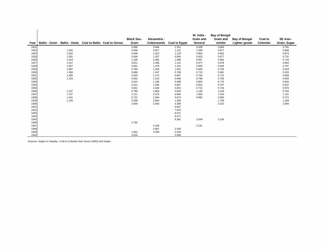
Year Baltic - Grain Baltic - Deals Coal to Baltic Coal to GenoaBlack Sea -

GrainAlexandria - Cottonseeds Coal to Egypt

W. India - Grain and General

Bay of Bengal -Grain and

similarBay of Bengal -Lighter goods

Coal to Colombo

SE Asia - Grain, Sugar

1922 0.896 0.946 1.351 0.938 0.883 0.7811923 1.535 0.908 0.957 1.131 1.090 0.877 0.8481924 1.552 0.846 1.022 1.119 0.964 0.962 0.8731925 1.361 0.806 1.307 0.994 0.923 0.877 0.7311926 1.519 1.166 2.585 1.098 0.997 0.962 0.7441927 1.547 0.812 1.456 1.131 0.977 0.978 0.8041928 1.507 0.661 1.278 1.101 0.900 0.844 0.7971929 1.687 0.780 1.426 1.051 0.825 0.709 0.6181930 1.569 0.666 1.307 0.708 0.719 0.581 0.5261931 1.305 0.643 1.174 0.667 0.764 0.714 0.6581932 1.125 0.592 1.233 0.649 0.786 0.756 0.6331933 0.614 1.196 0.598 0.802 0.770 0.6201934 0.612 1.255 0.667 0.813 0.797 0.6371935 0.651 1.040 0.815 0.715 0.744 0.5791936 1.237 0.785 1.864 0.643 1.149 1.043 0.7841937 1.707 1.211 2.375 0.994 1.300 1.343 1.1011938 1.161 0.721 1.564 0.673 0.883 0.983 0.7721939 1.145 0.936 2.844 1.429 1.759 1.2091940 2.600 5.550 4.369 2.515 2.9491941 6.6671942 7.6191943 8.5711944 8.5711945 6.381 3.346 3.1591946 2.7921947 5.259 2.2311948 4.567 2.4291949 1.831 3.359 2.5361950 3.016 3.006

Sources: Angier in Fairplay ; Coal to Colombo from Jevon (1962) and Angier.

Table 2: Nominal Freight Rate Indices - Atlantic Routes (1884 = 1.00)

Year

E. Latin America -

Grain

W. Latin America -

NitrateCoal to E.

Latin AmericaCoal to W.

Latin America

E. North America -

Timber

E. North America -

Grain

W. North America -

Grain

N. America Gulf Coast -

Cotton

N. America Gulf Coast -

Timber

N. America Gulf Coast -

Grain

Western Mediterranean

- Ore1869 1.122 1.016 1.376 2.139 1.447 1.762 1.792 1.250 1870 0.941 1.184 1.213 1.428 1.421 1.651 1.577 1.217 1871 1.164 1.421 1.276 1.487 1.474 1.778 1.385 1.225 1.7371872 1.219 1.474 1.394 1.679 1.553 4.460 2.077 1.317 1873 1.295 1.605 1.570 1.567 2.026 2.058 2.346 1.725 2.4431874 1.219 1.647 1.344 1.572 2.053 1.857 2.092 1.625 1875 1.233 1.395 1.109 0.914 1.952 1.462 1876 1.144 1.289 1.063 1.032 1.675 1.669 1.8051877 1.061 1.211 1.032 0.995 1.683 1.192 1.6281878 0.974 0.947 1.032 0.909 1.683 1.269 1.292 1879 0.949 1.000 1.063 0.947 1.476 1.462 1.249 1.1261880 1.077 1.105 1.077 0.979 1.397 1.723 1.142 1.3981881 1.103 1.237 1.027 0.904 1.127 2.269 1.055 1882 1.103 1.382 1.086 0.952 1.302 1.615 1.185 1.3571883 0.974 1.026 1.090 0.984 1.289 1.206 1.192 1.077 1.2231884 1.000 1.000 1.000 1.000 1.000 1.000 1.000 1.000 1.000 1.000 1.0001885 0.923 0.737 0.873 0.979 0.956 0.921 0.948 1.050 0.981 0.9571886 0.821 0.689 0.801 0.941 0.873 1.048 0.862 0.872 1.050 0.911 0.9371887 1.000 0.789 0.873 0.973 0.861 0.857 0.776 0.882 0.850 0.820 1.1431888 0.981 0.842 1.113 1.471 1.165 1.143 0.862 1.071 1.025 1.058 1.3891889 1.140 0.921 1.412 1.390 1.316 1.334 0.931 1.108 1.400 1.167 1.2701890 1.257 0.989 1.050 1.310 0.924 1.162 1.086 0.819 1.163 0.999 1.2681891 1.523 0.816 0.801 0.588 0.867 1.143 1.034 0.872 1.000 0.938 1.2051892 1.234 0.395 0.724 0.615 0.886 1.104 0.724 0.729 1.013 0.912 1.0041893 1.084 0.722 0.692 0.781 0.851 0.877 0.707 0.820 1.025 0.754 1.0841894 1.140 0.674 0.543 0.615 0.826 0.975 0.734 0.850 1.013 0.833 1.2131895 0.986 0.571 0.516 0.599 0.838 0.936 0.862 0.729 1.013 0.949 1.1281896 0.877 0.533 0.647 0.722 0.851 1.131 0.690 0.729 1.013 0.991 1.3381897 0.819 0.732 0.679 0.722 0.826 1.053 0.821 0.702 0.975 0.953 1.2131898 1.049 0.825 0.724 0.829 0.951 1.150 0.801 0.808 1.225 1.189 1.3641899 1.333 0.852 0.543 0.829 0.926 0.988 1.002 0.765 1.119 1.086 1.2291900 1.153 1.007 0.787 0.802 1.176 1.208 1.202 0.870 1.213 1.347 1.5431901 0.894 0.775 0.575 0.781 0.876 0.760 1.134 0.599 0.975 0.889 1.1281902 0.811 0.581 0.498 0.481 0.751 0.604 0.809 0.508 0.825 0.789 1.1861903 0.931 0.442 0.421 0.727 0.813 0.682 0.541 0.536 0.831 0.753 1.1411904 1.008 0.597 0.376 0.508 0.726 0.760 0.654 0.492 0.838 0.720 1.0591905 0.787 0.570 0.457 0.508 0.738 0.799 0.714 0.547 0.800 0.792 1.1781906 0.752 0.542 0.588 0.561 0.701 0.780 0.779 0.547 0.813 0.711 1.1931907 0.794 0.457 0.579 1.016 0.801 0.689 1.026 0.552 0.819 0.745 1.1301908 0.711 0.457 0.452 0.775 0.565 0.809 0.481 0.769 0.678 0.9811909 0.624 0.527 0.462 0.695 0.572 0.807 0.547 0.731 0.612 1.0111910 0.624 0.554 0.665 0.717 0.543 0.840 0.564 0.769 0.679 1.1101911 0.674 0.585 0.774 0.952 0.741 0.988 0.800 0.681 1.1711912 1.241 0.756 0.896 1.134 1.053 1.261 1.194 1.096 1.4241913 1.053 0.783 0.756 1.150 0.897 1.261 1.006 0.921 1.2271914 1.309 0.713 0.677 1.442 1.093 0.950 0.856 1.1341915 3.482 1.875 1.444 2.577 3.859 2.521 2.536 2.250 0.849 3.0251916 6.222 3.642 2.493 5.904 5.823 4.414 5.050 1.034 4.2541917 16.285 4.604 5.120 11.110 8.428

Year

E. Latin America -

Grain

W. Latin America -

NitrateCoal to E.

Latin AmericaCoal to W.

Latin America

E. North America -

Timber

E. North America -

Grain

W. North America -

Grain

N. America Gulf Coast -

Cotton

N. America Gulf Coast -

Timber

N. America Gulf Coast -

Grain

Western Mediterranean

- Ore1918 11.477 6.379 2.312 6.7831919 10.314 5.919 1.838 6.054 4.054 3.700 9.266 4.6881920 5.926 2.486 0.756 4.954 3.470 3.880 2.950 3.099 6.1221921 1.834 1.480 0.682 2.502 1.054 1.999 1.950 1.549 2.1971922 1.457 0.898 0.606 1.401 1.053 1.126 1.350 0.913 1.8151923 1.178 0.881 0.767 1.376 0.930 1.059 1.313 0.811 1.8061924 1.385 0.743 0.536 1.401 1.037 1.055 1.333 0.887 1.7141925 1.038 0.684 0.519 1.276 0.846 1.029 1.275 0.763 1.6011926 1.715 0.697 0.626 1.251 1.504 1.059 1.013 0.796 1.9911927 1.426 0.845 0.553 1.426 0.852 1.029 1.319 0.787 1.4721928 1.214 0.691 0.389 1.256 0.987 0.937 1.125 0.708 1.4631929 1.020 0.671 0.375 1.516 0.758 0.844 1.169 0.656 1.5801930 0.851 0.605 0.389 1.351 0.536 0.622 1.088 0.476 1.2961931 0.988 0.618 0.378 1.076 0.545 0.692 0.950 0.475 1.1751932 0.904 0.602 0.367 1.038 0.580 0.633 0.684 1.1821933 0.846 0.579 0.395 1.001 0.501 0.585 0.669 1.2651934 0.850 0.503 0.474 1.051 0.473 0.581 0.651 1.2651935 0.865 0.520 0.496 1.051 0.564 0.552 0.672 1.3491936 1.209 0.487 0.677 1.251 0.655 0.744 0.795 1.9101937 1.633 1.523 1.826 1.250 1.103 1.081 2.9251938 1.314 1.714 1.301 0.952 0.792 0.748 2.0161939 2.001 2.143 2.052 2.453 1.174 1.662 5.4971940 5.509 2.571 6.004 4.173 2.773 3.922 13.1321941 2.571 1942 2.205 1943 1944 1945 1.128 3.782 3.243 3.437 9.7731946 1.776 3.449 2.840 3.471 9.5201947 2.641 1.827 3.599 2.898 3.766 8.8771948 2.325 2.998 2.647 3.310 7.9301949 2.111 2.816 2.025 4.135 6.9371950 1.546 3.280 2.812 3.258 7.870

Sources: Angier in Fairplay ; W. Latin America Nitrate before 1890 from Stemmer (1989); E. Latin America Grain before 1880 from Harley (1989); Coal to Latin America from Jevons (1962) and Angier.

Table 3: Global Nominal and Real Freight Rate Indices (1884 = 1.00)

Year Nominal IndexDeflated by

Sauerbeck/RPIDeflated by

Commodities1870-1874 1.88 1.29 1.231875-1879 1.53 1.22 1.241880-1884 1.24 1.09 1.15

1884 1.00 1.00 1.001885-1889 1.05 1.12 1.111890-1894 0.87 0.93 0.821895-1899 0.87 1.00 0.921900-1904 0.81 0.82 0.691905-1909 0.74 0.67 0.651910-1914 0.94 0.78 0.761915-1919 6.79 2.85 2.281920-1924 1.89 0.75 0.601925-1929 1.05 0.58 0.591930-1934 0.78 0.63 0.551935-1939 1.27 0.97 0.771940-1944 2.98 2.49 1.001945-1949 2.41 0.95 0.571950-1954 2.21 0.63 0.361955-1959 2.72 0.60 0.551960-1964 2.00 0.39 0.431965-1969 2.03 0.33 0.431970-1974 2.84 0.33 0.441975-1979 3.16 0.18 0.361980-1984 3.95 0.13 0.371985-1989 3.90 0.10 0.451990-1994 4.32 0.08 0.411995-1997 4.44 0.08 NA

Sources: Data for 1870-1950 from Angier. Fairplay;Rates after 1950 from Hummels (1999). For construction of Global Index, see text. Real Indices deflated by Sauerbeck-Statist Index till 1950, by UK RPI thereafter.

Table 4: TFP Growth before World War IENA Alexandria Riga Bombay

Distancefrom UK

1871/3 – 1887/9Average ChangeIn NominalFreight Rates -2.23% -2.56% -2.93% -3.03%

Contribution of:Wages 2.16% 1.88% 1.64% 1.59%Ship Prices 33.1% 28.8% 25.1% 24.3%Coal Prices 30.2% 25.4% 24.5% 20%

Average TFP change 0.76% 1.12% 1.43% 1.64%

1887/9 – 1909/11

Average ChangeIn NominalFreight Rates -1.92% -1% -1.63% -2.12%

Contribution of:Wages -3.5% -6.76% -4.2% -3.2%Ship Prices 23.1% 44.3% 27.4% 21%Coal Prices -1.4% -20.8% -10.2% 9%

Average TFP change 1.58% 0.84% 1.94% 1.55%

Sources: Appendix 4 for Factor Prices. Factor shares are as follows: Coal 28.6%, Capital costs 57.1%,Wages 14.3%. Port costs and other factors have not been included for lack of data. See Appendix 4.

Table 5: TFP Growth in the Interwar PeriodENA Alexandria

Distancefrom UK

1909/11-1932/4Average Change In NominalFreight Rates -1.39% 1%

Contribution of:Wages -100.84% 54.55%Ship Prices -268.9% 145%Coal Prices -53.4% 27.1%

Average TFP change 2.83% 1.27%

1923/5-1932/4

Average ChangeIn NominalFreight Rates -3.61% -1.39%

Contribution of:Wages 1.98% 5.17%Ship Prices 48% 124%Coal Prices 23.43% 72.3%

Average TFP change 0.96% -1.4%

Sources: Appendix 4 for Factor Prices. Factor shares are as follows: Coal 28.6%, Capital costs 57.1%,Wages 14.3%. Port costs and other factors have not been included for lack of data. See Appendix 4.

Table 6: Explaining TFP Growth before World War IENA Alexandria Riga Bombay

Distancefrom UK

A. 1871/3 – 1887/9

Contribution toTFP Growth:

Ship Size 30.8% 32.5% 59.4% 25.9%Load Capacity 60.9% 39.0% 30.55% 28.57%Coal Consumed 13.4% 12.37% 15.93% 11.68%No. of Seamen 33.6% 18.01% 9.6% 12.31%Time at Sea -19.34% 2.01% 15.44% 75.91%Time at Port 14.7% 27.34% 19.7% 38.1%

Percentage of TFPExplained 133.5% 131.2% 150% 192.4%

B. 1887/9 – 1909/11

Contribution toTFP Growth:

Ship Size 28.4% 76.1% 86.62% 47.98%Load Capacity 21.5% 37.9% 22.48% 21.94%Coal Consumed -3.45% -20.97% 34.93% -11.33%No. of Seamen 4.9% -2.01% -19.03% -1.53%Time at Sea -7.86% -18.37% 7.89% -38.62%Time at Port 33.1% 29.76% -18.39% -10.38%

Percentage of TFPExplained 76.7% 101.57% 114.5% 7.95%

Sources, see text. For calculations, see Appendix 5.

Figure 1A: Nominal Freight Rate Indices 1869-1913(1884=1.00)

0.6

0.8

1

1.2

1.4

1.6

1.8

1869 1874 1879 1884 1889 1894 1899 1904 1909 1914

Global

Isserlis

Isserlis 5-year avg

Sources: Table 3 and Isserlis (1938).

Index

Figure 1B: Nominal Freight Rate Indices 1920-1937(1884=1.00)

0

1

2

3

4

5

6

7

8

9

10

11

12

1917 1919 1921 1923 1925 1927 1929 1931 1933 1935 1937

Global Index

Isserlis

Isserlis 5-year avg

Sources: Table 3 and Isserlis (1938).

Index

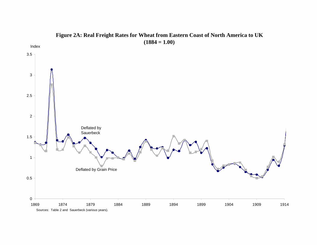
0

0.5

1

1.5

2

2.5

3

3.5

1869 1874 1879 1884 1889 1894 1899 1904 1909 1914

Figure 2A: Real Freight Rates for Wheat from Eastern Coast of North America to UK (1884 = 1.00)

Sources: Table 2 and Sauerbeck (various years).

Index

Deflated by Grain Price

Deflated by Sauerbeck

0

0.5

1

1.5

2

2.5

1869 1874 1879 1884 1889 1894 1899 1904 1909 1914

Deflated by Sauerbeck

Deflated by Jute Price

Figure 2B: Real Freight Rates for Jute from Calcutta to UK (1884=1.00)

Sources: Table 1 and Sauerbeck (various years)

Index

Figure 3: Global Nominal Freight Rates 1870-1997(1884 = 1.00)

0

1

2

3

4

5

6

7

1870 1880 1890 1900 1910 1920 1930 1940 1950 1960 1970 1980 1990 2000Sources: Table 3 and Hummels (1999).

Index

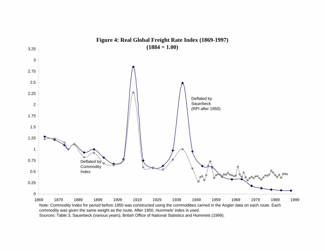
Figure 4: Real Global Freight Rate Index (1869-1997)(1884 = 1.00)

0

0.25

0.5

0.75

1

1.25

1.5

1.75

2

2.25

2.5

2.75

3

3.25

1869 1879 1889 1899 1909 1919 1929 1939 1949 1959 1969 1979 1989 1999Note: Commodity Index for period before 1950 was constructed using the commodities carried in the Angier data on each route. Each commodity was given the same weight as the route. After 1950, Hummels' index is used.Sources: Table 3, Sauerbeck (various years), British Office of National Statistics and Hummels (1999).

Deflated by Commodity Index

Deflated by Sauerbeck (RPI after 1950)