natural neighbour petrov-galerkinmethod for shape design ... · natural neighbour...

Copyright c© 2008 Tech Science Press CMES, vol.26, no.2, pp.107-121, 2008

Natural neighbour Petrov-Galerkin Method for Shape DesignSensitivity Analysis

Kai Wang1, Shenjie Zhou1,2, Zhifeng Nie1 and Shengli Kong1

Abstract: The natural neighbour Petrov-Galerkin method (NNPG) is one of the spe-cial cases of the generalized meshless localPetrov-Galerkin method (MLPG). This paperdemonstrates the NNPG can be successfully usedin design sensitivity analysis in 2D elasticity.The design sensitivity analysis method based onthe local weak form (DSA-LWF) in the NNPGcontext is proposed. In the DSA-LWF, the localweak form of governing equation is directlydifferentiated with respect to design variablesand discretized with NNPG to obtain the sensi-tivities of structural responds. The calculationof derivatives of shape functions with respectto design variables is avoided. No backgroundmeshes are needed to integrate the weak form, noassembly process is needed to generate the globalstiffness matrix and no user-defined parametersare used as well. Three numerical examples aresolved using DSA-LWF and the results show theproposed method gives very accurate solutionsfor these problems.

Keyword: shape design sensitivity analysis;meshless method; Petrov-Galerkin method; nat-ural neighbour interpolation

1 Introduction

Gradient-based methods are widely used in shapeoptimization problems. In these methods, theshape design sensitivity analysis (DSA) is con-cerned with finding the variation of structural re-sponses (displacement, stresses, etc.) with respectto design variables, which describe the geome-try of the domain [Lacroix and Bouillard (2003)].

1 School of Mechanical Engineering, Shandong University,No.73 Jingshi Road, Jinan, 250061, P. R. China

2 Corresponding author. Email: [email protected]

These sensitivities are needed in order to providethe gradients of the objective function or con-straints. An accurate computation of sensitivityinformation plays a critical role in the shape opti-mization and can reduce the computational costs[Kim, Choi and Botkin (2003)].

There are several methods which can be employedin design sensitivity analysis. Generally, there arefour different types, namely finite difference, dis-crete, continuum, and computational derivatives.Among these methods, the continuum-based DSAmethod is widely used in design sensitivity anal-ysis and shape optimization problems [Lacroixand Boouillard (2003); Kim, Choi and Botkin(2003); Bobaru and Mukherjee (2001); Bobaruand Mukherjee (2002); Grindeanu, Kim, Choi andChen (2002); Kim, Yi and Choi (2002); Chang,Choi, Tsai, Chen, Choi and Yu (1995)]. In thiskind of method, the continuous deformation of thestructure is simulated and the material derivativeconcept is used to define the sensitivities of struc-tural responds.

The finite element methods (FEMs) have becomethe most popular numerical approach in variousengineering applications. However, the FEMs arenot convenient for shape optimization problemsdue to the use of mesh. Firstly, the remeshing pro-cess is often inevitable in optimization iterationswhen the mesh gets distorted too much. Secondly,it is necessary to modify the geometry and to gen-erate a new mesh in order to compute the sensi-tivities. Unfortunately, for most of the existingmethods, a restriction is that the perturbed meshmust have the same topology as the initial one.This can not be satisfied if the mesh is generatedwith the aim of controlling its accuracy [Lacroixand Bouillard (2003)].

Meshless methods [Belytschko, Krongauz, Or-

108 Copyright c© 2008 Tech Science Press CMES, vol.26, no.2, pp.107-121, 2008

gan, Fleming and Krysl (1996); Atluri and Zhu(1998); Cueto, Sukumar, Calvo, Cegoñino andDoblaré (2003); Liu, Jun, Zhang (1995)] as al-ternative methods to FEMs have attracted muchattention these years. As the approximation of so-lution variables is constructed by scattered nodesinstead of elements, meshless methods are moresuitable for moving boundary problems, largedeformation problems, high speed impact prob-lems, etc. With regard to the DSA computa-tion and shape optimization, because no meshis needed to interpolate either field variables ortheir sensitivities, the aforementioned inconve-niences of use of FEM are resolved. Many re-searchers take the advantages of meshless meth-ods in DSA computations [Lacroix and Boouil-lard (2003); Kim, Choi and Botkin (2003); Bo-baru and Mukherjee (2001); Bobaru and Mukher-jee (2002); Grindeanu, Kim, Choi and Chen(2002)]. Lacroix and Bouillard (2003) proposeda DSA approach by coupling the element freeGalerkin method (EFG) [Belytschko, Lu and Gu(1994)] with the FEM. Bobaru and Mukherjee(2001, 2002) developed a continuum-based DSAmethod in the EFG context and used in shapeoptimization problems of both linear elastic andthermo elastic solids. In their method, the deriva-tive of global Galerkin weak form of equilib-rium equation with respect to each design vari-able is computed by direct differentiation method(DDM) [Kim, Choi and Botkin (2003); Bobaruand Mukherjee (2001); Bobaru and Mukherjee(2002); Grindeanu, Kim, Choi and Chen (2002)].Numerical methods for continuum-based shapedesign sensitivity analysis and optimization us-ing reproducing kernel particle method (RKPM)[Liu, Jun and Zhang (1995)] were proposed byGrindeanu, Kim, Choi and Chen (2002) and Kim,Yi and Choi (2002).

Many meshless methods have been developed sofar. Among these methods, the meshless localPetrov-Galerkin method (MLPG) originally pro-posed by Atluri and Zhu (1998) is one of the mostprominent methods, because it is not only a trulymeshless method but also a generalized frame-work that could be used to derive other mesh-less methods [Atluri, Kim and Cho (1999); Atluri

and Shen (2002)]. Many researchers are opti-mistic about this method and use it in their re-search fields. In recent years, the MLPG hasmade great progress in many aspects. Several newmethods are proposed within the framework ofMLPG [Atluri and Shen (2002); Atluri, Liu andHan (2006a); Atluri, Liu and Han (2006b); Atluri,Han and Rajendran (2004); Vavourakis, Selloun-tos and Polyzos (2006); Vavourakis and Polyzos(2007)]. A wide variety of engineering problemsare solved by the MLPG type meshless methods[Han and Atluri (2004); Shen and Atluri (2004);Andreaus, Batra and Porfiri (2005); Han, Rajen-dran and Atluri (2005); Han, Liu, Rajendran et al.(2006); Ching and Chen (2006); Gao, Liu and Liu(2006); Sladek, Sladek and Zhang et al. (2007);Jarak, Soric and Hoster (2007)].

The natural neighbour Petrov-Galerkin method(NNPG) [Wang, Zhou and Shan (2005)] is oneof the special cases of the generalized MLPG.As this method is quite efficient and easy to im-plement, it is suitable for DSA computation andshape optimization where high efficiency is de-sired. This paper demonstrates the NNPG can besuccessfully used for DSA computation and shapeoptimization in 2D elasticity. The design sensi-tivity analysis method based on the local weakform (DSA-LWF) in the NNPG context is pro-posed. The material derivative concept is adoptedin the DSA-LWF, and the continuous formula-tion of design sensitivity analysis is derived by di-rectly differentiating the local weak form of equi-librium equations. The discretization of the con-tinuous formulation and the numerical implemen-tation are also proposed. Three numerical exam-ples are presented to test the validity and accuracyof the DSA-LWF method.

This paper is organized as follows: In section2, the natural neighbour Petrov-Galerkin methodis briefly reviewed. In section 3, the DSA-LWFmethod under the NNPG framework is proposedin details. In section 4, three numerical examplesare presented to test the proposed method. Thispaper ends with the conclusions in section 5.

Natural neighbour Petrov-Galerkin Method 109

2 Review of natural neighbour Petrov-Galerkin method

Under the framework of MLPG, new meshlessmethod can be derived if the trial function, testfunction and integration method are carefully cho-sen [Atluri, Kim and Cho (1999); Atluri and Shen(2002)]. The natural neighbour Petrov-Galerkinmethod (NNPG) [Wang, Zhou and Shan (2005)]can be considered as a special case of MLPG. Thismethod is developed to alleviate the task of impo-sition of essential boundary condition in classicalMLPG. In the NNPG, the non-Sibsonian interpo-lation is used to approximate the trial function,and linear FEM shape function is chosen to be thetest function. The Delaunay tessellation is used toconstruct the nodal local sub-domain Ωs, which iscoincident with the support of nodal test function.

In each nodal local sub-domain Ωs, the localPetrov-Galerkin method [Atluri and Zhu (1998)]is used in stead of global Galerkin one. As non-Sibsonian interpolation is used to approximate thefield variables, neither penalty parameters [Atluriand Zhu (1998)] nor Lagrange multipliers [Be-lytschko, Lu and Gu (1994)] are needed to imposethe essential boundary condition. The NNPG con-tinuous local weak form of governing equation inelasto-statics is defined as:

∫Ωs

σi jNIi, jdΩ−∫Lu

NIiσi jn jdΓ

=∫Ωs

NIibidΩ+∫Lt

NIit idΓ (1)

where ∂Ωs = Lu + Lt + Ls is the boundary of lo-cal sub-domain, σi jis the stress tensor related tothe displacement field ui, biis the vector of bodyforce, n j is the unit outward normal vector tothe boundary Lu, ti is the prescribed tractions onthe traction boundaryLt and NIi is the test func-tion corresponding to the nodal sub-domain Ωs.To obtain the discrete algebraic equation, the dis-placement of point x is approximated by:

uh(x) =n

∑I=1

φI(x)uI (2)

with

φI(x) =sI(x)/hI(x)

∑nJ=1 [sJ(x)/hJ(x)]

(3)

where n is the number of natural neighbours of thepoint x, uI (I=1, 2,. . . , n) are the vectors of nodaldisplacements at n natural neighbours, and φI(x)isthe non-Sibsonian interpolation shape function, sI

is the Lebesgue measure of the Voronoi bound-ary associated with node I(here is the length ofVoronoi edge in 2D case), and the hI is the dis-tance between the evaluated point x and the nodeI.

The discrete form can be obtained by substitutingequation (2) into it equation (1):

N

∑J=1

KIJuJ = FI , I = 1,2, . . .,N (4)

where KIJ and FI are local stiffness matrix andforce matrix corresponding to the nodal sub-domain ΩI

S, N is the total number of the nodes inthe global domain and on its boundary, uJ is thematrix of nodal displacements.

As a special case of the generalized MLPG, theNNPG inherits the virtues of the MLPG [Atluri,Kim and Cho (1999)], e.g., no assembly processis needed to form the global stiffness matrix andno additional background cells are needed to in-tegrate the weak form. Compare with the classi-cal MLPG, the NNPG has two additional proper-ties [Wang, Zhou and Shan (2005)]. Firstly, thecalculation of non-Sibsonian interpolation shapefunction is more efficient than that of MLS, andthe shape function has Kronecker Delta functionproperty. This may contribute to its high effi-ciency. Secondly, by virtue of the test functionused, the supports of integrands align with the in-tegration domains. This may improve the accu-racy of numerical integration [Dolbow and Be-lytschko (1999)]. All these properties, no matterinherited or intrinsic, render the NNPG a promis-ing method for DSA computation and shape opti-mization.

3 Local continuum-based DSA formulation

The sensitivity of a structural response (displace-ment, stress) with respect to a design variable is a


kind of material derivative [Bobaru and Mukher-jee (2001), Kim, Yi and Choi (2002)] which takesinto account the shape variation of the structuraldomain due to the design variable perturbation.Let us consider the displacement vector u whichcan be expressed as a function of the design vari-able τττ and of the position ξξξ . The sensitivity ofu with respect to τττ is defined as [Bobaru andMukherjee (2001)]:

u = limτττ→0

u[ξξξ (x,τττ),τττ]−u(x,0)τττ

= u′ +∇u.v (5)

In above equation, v(x) is the design velocityfield [Ródenas, Fuenmayor and Tarancón, J. E.(2004)], which defines the variation of the po-sition of each material point due to the varia-tion of the design variable. By importing strain-displacement relation and constitutive equation[Timoshenko and Goodier (1970)], all other sensi-tivities (e.g., stress sensitivities σσσ) can be derivedfrom the displacement sensitivity u.

3.1 Continuous DSA formulation based onNNPG local weak form

There are several methods can be used to calculatethe displacement sensitivity. Among these meth-ods, the direct differentiation method (DDM) isquite simple and widely used in shape optimiza-tion problems [Kim, Choi and Botkin (2003); Bo-baru and Mukherjee (2001); Bobaru and Mukher-jee (2002); Grindeanu, Kim, Choi and Chen(2002)]. Consider a structural system in the fi-nal equilibrium configuration, corresponding to agiven design variableτττ. The equilibrium equationfor the structural system can be written as:

A(τττ)u(τττ) = f(τττ) (6)

The displacement field u can be solved fromabove equation. By using DDM, the displacementsensitivity u is obtained by directly differentiat-ing equation (6) with respect to every design vari-ables:

A(τττ)u =df(τττ)

dτττ− dA(τττ)

dτττu(τττ) (7)

As global Galerkin method dominates in numeri-cal methods, almost all the continuum-based DSA

formulations are derived from it. In this case,the equation (6) is a global symmetric weak formof equilibrium equation. After using DDM, theequation (7) includes integrals over global do-main. These integrals have to be evaluated withthe aid of background meshes [Belytschko, Kro-ngauz, Organ, Fleming and Krysl (1996)]. It isreported that the support of the integrand needs tobe aligned with the background mesh to improvethe accuracy of Gaussian quadrature [Dolbow andBelytschko (1999)]. However, to construct back-ground meshes aligning with the supports of in-tegrands is not easy for most meshless methods.Therefore, integration error is often introduced. Inaddition, the “assembly” process is always neces-sary to generate the stiffness matrix in these meth-ods [Atluri and Zhu (1998)].

Under the framework of NNPG, the local weakform is used instead of global Galerkin one and amore explicit form of equation (7) is obtained bydirectly differentiating the continuous local weakform of governing equation (1). For example, thematerial derivative of first term in the left hand ofthe equation (1) is calculated:

∫Ωs

[ ˙(σi j(u)NIi, j)+(σi j(u)NIi, j)(vi,i)]dΩ =

∫Ωs

[σi j(u)NIi, j +σi j(u) ˙NIi, j +σi j(u)NIi, j(vi,i)]dΩ

(8)

where ˙NIi, j = NIi, j − NIi,kvk, j is the materialderivative of the spatial derivative of the test func-tion. σi j is the stress sensitivity, which can be ob-tained by importing strain-displacement relationand constitutive law:

σi j(u) = σi, j(u)− 12

Di jkl(vk, jui,k +vk,iu j,k) (9)

where Di jkl is the material constant tensor. Substi-tuting equation (9) into equation (8), the materialderivative of first term in the left hand of the equa-


tion (1) can be written as:

∫Ωs

[˙(σi j(u)NIi, j)+(σi jNIi, j)(vi,i)

]dΩ

=∫Ωs

σi j(u)NIi, jdΩ

− 12

∫Ωs

Di jkl(vk, jui,k +vk,iu j,k

)NIi, jdΩ

+∫Ωs

σi j(u)(NIi, j −NIi,kvk, j)dΩ

+∫Ωs

σi j(u)NIi, j(vi,i)dΩ (10)

With similar procedures, the material derivative ofequation (1) can be written as:

∫Ωs

σi j(u)NIi, jdΩ

− 12

∫Ωs

Di jkl[vk, jui,k +vk,iu j,k]NIi, jdΩ

−∫Ωs

σi j(u)NIi,kvk, jdΩ

+∫Ωs

σi j(u)(vi,i)NIi, jdΩ

−n j

∫Lu

σi j(u)NIidΓ

+n j

2

∫Lu

Di jkl[vk, jui,k +vk,iu j,k]NIidΓ

−∫Lu

σi j(u)n jNIi(vini)HdΓ =

∫Ωs

[bi +bi(vi,i)]NIidΩ +∫Lt

[t i + t i(vini)H]NIidΓ

(11)

where H = −ni,i is the surface divergence [Bo-baru and Mukherjee (2001)]. In above equation,considering strain-displacement relation and con-stitutive law of elasto-statics, the local continuous

DSA formulation is obtained:

∫Ωs

Di jkl12(uk,l + ul,k)NIi, jdΩ

− 12

∫Ωs

Di jkl[vk, jui,k +vk,iu j,k]NIi, jdΩ

−∫Ωs

Di jkl12(uk,l +ul,k)NIi,kvk, jdΩ

+∫Ωs

Di jkl12(uk,l +ul,k)(vi,i)NIi, jdΩ

−n j

∫Lu

Di jkl12(uk,l + ul,k)NIidΓ

+n j

2

∫Lu

Di jkl[vk, jui,k +vk,iu j,k]NIidΓ

−∫Lu

Di jkl12(uk,l +ul,k)n jNIi(vini)HdΓ =

∫Ωs

[bi +bi(vi,i)]NIidΩ +∫Lt

[t i + t i(vini)H]NIidΓ

(12)

3.2 NNPG discretization and numerical imple-mentation

To avoid the derivatives of shape functions withrespect to design variables, the displacementsensitivities are also approximated with non-Sibsonian interpolation:

uh(x) =n

∑I=1

φI(x)uI (13)

where φI is the non-Sibsonain interpolation shapefunction of natural neighbour I and uI are the vec-tors of fictitious nodal displacement sensitivity.Substituting equation (2) and (13) into equation(12), the discrete form of sensitivity formulation


is obtained:

∫Ωs

Di jkl12

(n

∑I=1

φI,l(x)uIk +n

∑I=1

φI,k(x)uIl

)

NIi, jdΩ

− 12

∫Ωs

Di jkl

[vk, j

(n

∑I=1

φI,k(x)uIi

)

+vk,i

(n

∑I=1

φI,k(x)uI j

)]NIi, jdΩ

−∫Ωs

Di jkl12

(n

∑I=1

φI,l(x)uIk +n

∑I=1

φI,k(x)uIl

)

NIi,kvk, jdΩ

+∫Ωs

Di jkl12

(n

∑I=1

φI,l(x)uIk +n

∑I=1

φI,k(x)uIl

)(vi,i)

NIi, jdΩ

−n j

∫Lu

Di jkl12

(n

∑I=1

φI,l(x)uIk +n

∑I=1

φI,k(x)uIl

)

NIidΓ

+n j

2

∫Lu

Di jkl

[vk, j

(n

∑I=1

φI,k(x)uIi

)

+vk,i

(n

∑I=1

φI,k(x)uI j

)]NIidΓ

−∫Lu

Di jkl12

(n

∑I=1

φI,l(x)uIk +n

∑I=1

φI,k(x)uIl

)

n jNIi(vini)HdΓ

=∫Ωs

[bi +bi(vi,i)

]NIidΩ

+∫Lt

[t i + t i(vini)H

]NIidΓ (14)

For simplicity, the matrix form of above equationscan be written as:

N

∑J=1

KIJuJ =N

∑J=1

(LIJ +MIJ)uJ +QI ,

I = 1,2, . . .,N (15)

where N is the total number of the nodes in theglobal domain and on its boundary, uJ is the ma-trix of nodal displacements, matrices KIJ , LIJ ,MIJ and QI are given by

KIJ =∫Ωs

VTdIDBJdΩ−

∫Lu

VINDBJdΓ (16)

LIJ =∫Ωs

VTdIDBJdΩ+

∫Ωs

VTdIDBJdΩ

−∫Ωs

VTdIDBJ divvdΩ (17)

MIJ =∫Lu

VINDBJ(v ·n)HdΓ−∫Lu

VINDBJdΓ

(18)

QI =∫Ωs

VI(b +bdivv

)dΩ

+∫Lt

VI

[t + t(v ·n)H

]dΓ (19)

It should be noted that the equation (16) is thesame as the equation (16) in Wang, Zhou andShan (2005). See Wang, Zhou and Shan (2005)for the explicit form of BJ , N, D, VI and VdI in2D elasto-statics problem. Matrices BJ and VdI

are defined:

BJ =

⎡⎣v1,1φJ,1 +v2,1φJ,2 0

0 v1,2φJ,1 +v2,2φJ,2

v1,2φJ,1 +v2,2φJ,2 v1,1φJ,1 +v2,1φJ,2

⎤⎦

(20)

VdI =

⎡⎣v1,1NI,1 +v2,1NI,2 0

0 v1,2NI,1 +v2,2NI,2

v1,2NI,1 +v2,2NI,2 v1,1NI,1 +v2,1NI,2

⎤⎦(21)

For 2D cases, equation (16) denotes two algebraicequations containing 2N unknown nodal displace-ment sensitivities for one sub-domain. Loop over


all the sub-domains, the global algebraic systemis obtained without ‘assembly’ process.

Ku = F′ (22)

In above equation, matrix F′ is called external fic-titious force [Bobaru and Mukherjee (2001)]. Ma-trix K is the global stiffness matrix same as thestiffness matrix of structural analysis. Thus, thestiffness matrix in structural analysis stage can bestored and used for DSA purpose, which can re-duce computational costs. By solving equation(22) for u, εεε(u) and σσσ (u) at any desired positioncan be approximated as:

εεε(u) =n

∑I=1

BI uI −n

∑I=1

BIuI (23)

σσσ(u) = Dε(u) (24)

From the equation (20)-(21), it is observed thatthe DSA results will strongly depend on the de-sign velocity field. Applying an inappropriate ve-locity field may lead to inaccurate DSA results.Although the velocity field for a given problemis not uniquely defined, the design velocity fieldmust meet both a regularity requirement and alinear dependency requirement [Ródenas, Fuen-mayor and Tarancón (2004)]. For regularity re-quirement, the C0 design velocity field with in-tegrable first derivatives is required. The lineardependency requirement states that the design ve-locity fields must linearly depend on the variationof shape. There are several methods for comput-ing the design velocity field. For example, bound-ary displacement method, isoparametric mappingmethod, Laplacian smoothing, exact differenti-ation of nodal co-ordinates and boundary meshmethod are commonly used. Comparisons be-tween these methods can be found in Ródenas,Fuenmayor and Tarancón (2004). The boundarydisplacement method [Chang, Choi, Tsai, Chen,Choi and Yu (1995); Ródenas, Fuenmayor andTarancón (2004)] is used in this work. Thismethod generates the velocity field by solving anauxiliary elasticity problem. As this method cansimulate the natural deformation of the continuumstructure, the obtained velocity field can be usedto update the nodal position in optimization itera-tions.

The numerical implementation of DSA-LWF isquite easy, and can be summarized as several ma-jor steps shown in table 1.

4 Numerical results

Three numerical examples are presented to testthe validity and accuracy of the proposed DSA-LWF approach. Three Gaussian points are usedto evaluate domain integrals over each Delaunaytriangle. For convergence study, the relative er-ror of sensitivities [Fuenmayor, Oliver and Ró-denas (1997); Ródenas, Fuenmayor and Tarancón(2004)] with respect to a given design variable αm

is defined:

ηm =

√∣∣∣∣χmathrmem −χn

m

χem

∣∣∣∣ (25)

where the superscripts e and n denote the ex-act solutions and numerical solutions, respec-tively. Andχm is the sensitivity of the displace-ment norm:

χm =∂ ‖u‖2

∂αm=

∂∂αm

⎛⎝∫

Ω

uT udΩ

⎞⎠ (26)

As the non-Sibsonian interpolation only have C0

continuity, a least square smoothing procedure isemployed to recover nodal stresses and their sen-sitivities. The GiD [http://gid.cimne.upc.es] isused to visualize the results in the third numeri-cal example.

4.1 The pulling of a bar

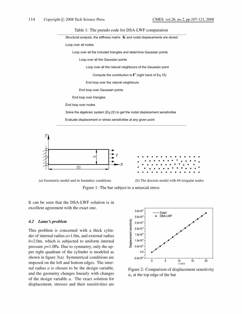
A bar with E = 3×107Pa and ν = 0.3 is subjectto a uniaxial stress t = 1.0×104Pa in the x direc-tion at the free end. The dimensions of the barand its boundary conditions are illustrated in fig-ure 1(a). In this problem, the length of the barl is chosen to be the design variable. A linearvelocity distribution is used. The exact solutionof displacement sensitivity is given in Bobaru andMukherjee (2001). In the computation, irregularnodal arrangement with 68 nodes is used as shownin figure 1(b). The numerical solution for the dis-placement sensitivity ux along the x at the top edgeare compared with the exact solution in figure 2.


Table 1: The pseudo code for DSA-LWF computation

Structural analysis, the stiffness matrix K and nodal displacements are stored

Loop over all nodes

Loop over all the included triangles and determine Gaussian points

Loop over all the Gaussian points

Loop over all the natural neighbours of the Gaussian point

Compute the contribution toF′ (right hand of Eq.15)

End loop over the natural neighbours

End loop over Gaussian points

End loop over triangles

End loop over nodes

Solve the algebraic system (Eq.22) to get the nodal displacement sensitivities

Evaluate displacement or stress sensitivities at any given point

(a) Geometric model and its boundary conditions (b) The discrete model with 68 irregular nodes

Figure 1: The bar subject to a uniaxial stress

It can be seen that the DSA-LWF solution is inexcellent agreement with the exact one.

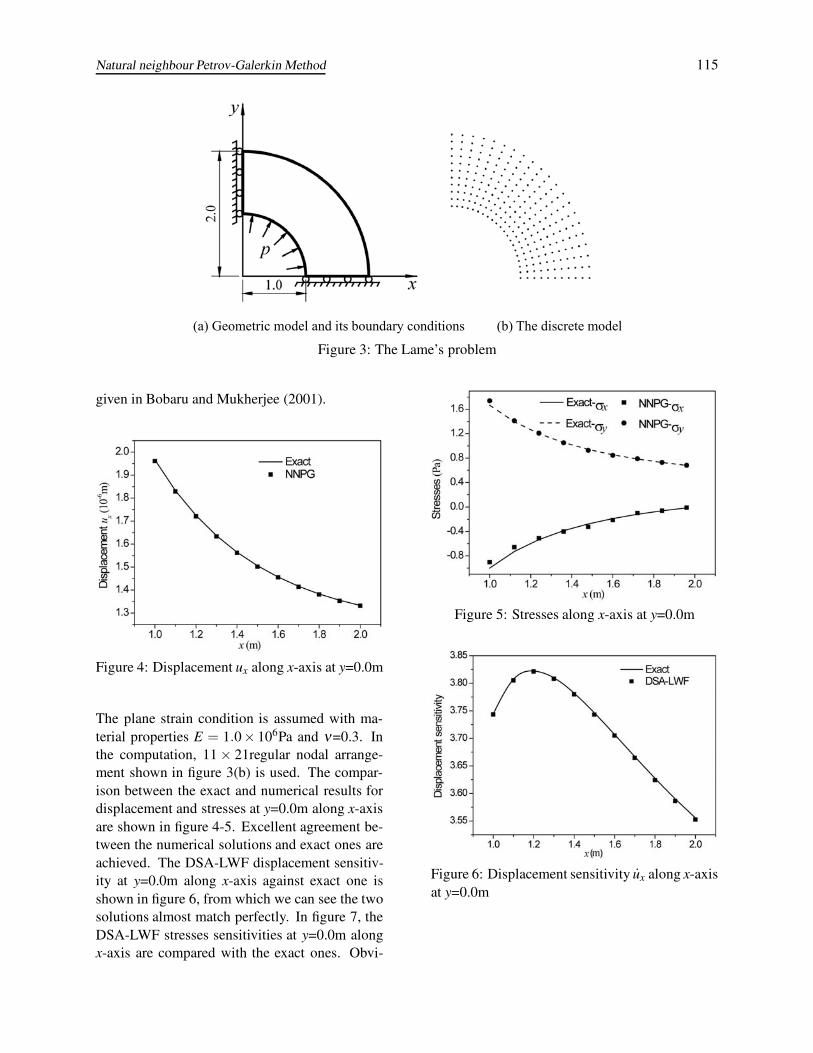
4.2 Lame’s problem

This problem is concerned with a thick cylin-der of internal radius a=1.0m, and external radiusb=2.0m, which is subjected to uniform internalpressure p=1.0Pa. Due to symmetry, only the up-per right quadrant of the cylinder is modeled asshown in figure 3(a). Symmetrical conditions areimposed on the left and bottom edges. The inter-nal radius a is chosen to be the design variable,and the geometry changes linearly with changesof the design variable a. The exact solution fordisplacement, stresses and their sensitivities are

Figure 2: Comparison of displacement sensitivityux at the top edge of the bar


(a) Geometric model and its boundary conditions (b) The discrete model

Figure 3: The Lame’s problem

given in Bobaru and Mukherjee (2001).

Figure 4: Displacement ux along x-axis at y=0.0m

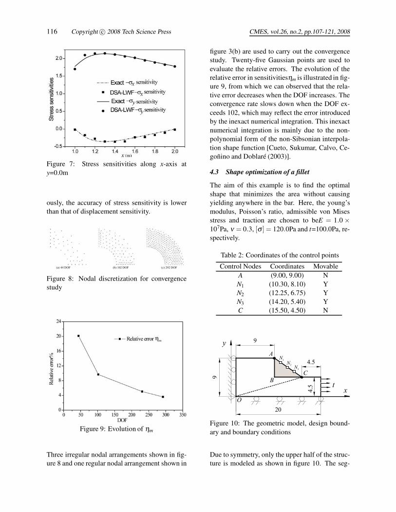
The plane strain condition is assumed with ma-terial properties E = 1.0× 106Pa and ν=0.3. Inthe computation, 11 × 21regular nodal arrange-ment shown in figure 3(b) is used. The compar-ison between the exact and numerical results fordisplacement and stresses at y=0.0m along x-axisare shown in figure 4-5. Excellent agreement be-tween the numerical solutions and exact ones areachieved. The DSA-LWF displacement sensitiv-ity at y=0.0m along x-axis against exact one isshown in figure 6, from which we can see the twosolutions almost match perfectly. In figure 7, theDSA-LWF stresses sensitivities at y=0.0m alongx-axis are compared with the exact ones. Obvi-

Figure 5: Stresses along x-axis at y=0.0m

Figure 6: Displacement sensitivity ux along x-axisat y=0.0m


Figure 7: Stress sensitivities along x-axis aty=0.0m

ously, the accuracy of stress sensitivity is lowerthan that of displacement sensitivity.

(a) 44 DOF (b) 102 DOF (c) 292 DOF

Figure 8: Nodal discretization for convergencestudy

Figure 9: Evolution of ηm

Three irregular nodal arrangements shown in fig-ure 8 and one regular nodal arrangement shown in

figure 3(b) are used to carry out the convergencestudy. Twenty-five Gaussian points are used toevaluate the relative errors. The evolution of therelative error in sensitivitiesηm is illustrated in fig-ure 9, from which we can observed that the rela-tive error decreases when the DOF increases. Theconvergence rate slows down when the DOF ex-ceeds 102, which may reflect the error introducedby the inexact numerical integration. This inexactnumerical integration is mainly due to the non-polynomial form of the non-Sibsonian interpola-tion shape function [Cueto, Sukumar, Calvo, Ce-goñino and Doblaré (2003)].

4.3 Shape optimization of a fillet

The aim of this example is to find the optimalshape that minimizes the area without causingyielding anywhere in the bar. Here, the young’smodulus, Poisson’s ratio, admissible von Misesstress and traction are chosen to beE = 1.0 ×107Pa, ν = 0.3, [σ ] = 120.0Pa and t=100.0Pa, re-spectively.

Table 2: Coordinates of the control points

Control Nodes Coordinates MovableA (9.00, 9.00) NN1 (10.30, 8.10) YN2 (12.25, 6.75) YN3 (14.20, 5.40) YC (15.50, 4.50) N

4.5

20

BC

4.5

9

9

1N2N

3N

x

y

t

A

O

Figure 10: The geometric model, design bound-ary and boundary conditions

Due to symmetry, only the upper half of the struc-ture is modeled as shown in figure 10. The seg-


ment AC is chosen to be the design boundary thatcan be varied during the optimization. Five con-trol points are used to model the design bound-ary, namely A, N1, N2, N3 and C. As shownin table 2, A and C are fixed, while N1, N2

and N3 are movable. The y-coordinates of mov-able points on the design boundary are chosen tobe the design variables, i.e., (y_N1, y_N2, y_N3).The initial values of design variables are (8.10,6.75, 5.40). With certain design parameterizationmethod [Kim, Choi and Botkin (2003); Chang,Choi, Tsai, Chen, Choi and Yu (1995)], the de-sign boundary can be expressed as the function ofdesign variables, i.e. p(y_N1,y_N2,y_N3). It is re-ported that the use of Akima spline interpolationas the design boundary representation can leadto the smooth design boundary after optimization[Bobaru and Mukherjee (2001)], and therefore theAkima spline interpolation is used in this work.As the minimization of the total area is equivalentto minimization of the area of triangle ΔABC, theobjective function is chosen to be the area of tri-angle ΔABC. The inequality g(y_N1,y_N2,y_N3)is that the maximum von Mises stress do not ex-ceed the given admissible stress [σ ]. The mathe-matical formulation of this optimization problemcan be written as:

minAΔABC =∫

AC

p(y_N1,y_N2,y_N3)dx−4.5×6.5

(27a)

s.t.g(y_N1,y_N2,y_N3) = 1− σmax

[σ ]≥ 0 (27b)

4.5 ≤ y_Ni ≤ 9.0, i = 1,2,3 (27c)

Figure 11: The discrete model with 339 irregularnodes

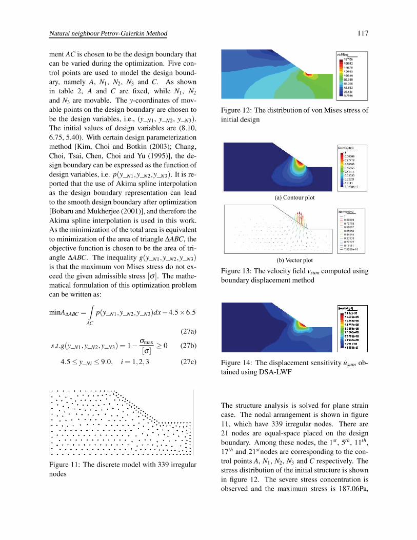
Figure 12: The distribution of von Mises stress ofinitial design

(a) Contour plot

(b) Vector plot

Figure 13: The velocity field vsum computed usingboundary displacement method

Figure 14: The displacement sensitivity usum ob-tained using DSA-LWF

The structure analysis is solved for plane straincase. The nodal arrangement is shown in figure11, which have 339 irregular nodes. There are21 nodes are equal-space placed on the designboundary. Among these nodes, the 1st , 5th, 11th,17th and 21stnodes are corresponding to the con-trol points A, N1, N2, N3 and C respectively. Thestress distribution of the initial structure is shownin figure 12. The severe stress concentration isobserved and the maximum stress is 187.06Pa,


Figure 15: Displacement sensitivity ux along theline OC

Figure 16: Displacement sensitivity uy along theline OC

which exceeds the admissible one by over fiftypercent. The design velocity field (vector sum)with respect to design variable y_N3 of the ini-tial design is shown in figure 13. As we can see,the velocity value at the control point N3 is unityand decreases to zero as the distance from thatcontrol point increases. The distribution of dis-placement sensitivity (vector sum) with respectto design variable y_N3 is illustrated in figure 14.The displacement sensitivity component ux and uy

along the line OC obtained by the DSA-LWF arecompared with those obtained by the finite differ-ence method (FDM, perturbation=0.001) in figure15-16, where perfect matches are observed.

Due to the nonlinear property of shape optimiza-tion problem, the Sequential Quadratic Program-

Figure 17: The iteration history

Figure 18: The final optimal design: The geomet-ric model, discrete model and the distribution ofvon-Mises stress of the optimal design

ming method (SQP) in Bobaru and Mukherjee(2001) is used to solve the minimization problem.In figure 17, the iteration history for the objec-tive function is illustrated. From this figure, wecan observe that the value of objective functionis decrease from 14.625m2 to 7.03m2 after onlyfour iterations, which is quite close to the opti-mal value, i.e., 6.98m2. The high convergencerate benefits from the accurate sensitivities ob-tained from DSA-LWF. In figure 18, the optimaldesign is illustrated, where no oscillating designboundary is observed. The severe stress concen-tration disappeared and there are 13 nodes outof 21 nodes on the design boundary whose vonMises stresses approach admissible one. Satis-fied result is obtained after the optimization eventhough only three design variables are used. Also,the optimization process is totally automatic, andabsolutely no remeshing processes are needed.


5 Conclusions

The design sensitivity analysis method based onthe local weak form (DSA-LWF) is proposed inthis paper. The numerical examples show the ob-tained DSA-LWF solutions are valid and accurate.This method possesses the following properties:

(1) No additional background meshes are neededto integrate the weak form and no assemblyprocess is needed to generate the global stiff-ness matrix because the local weak form isused instead of global weak form. No user-defined parameters (e.g., penalty parameterand size of supports of weight functions) areneeded.

(2) More accurate solution can be obtained, asthe differentiation is taken before the dis-cretization. The calculation of derivatives ofshape functions with respect to design vari-ables is avoided.

(3) Drawbacks related to the use of FEM areeliminated because the NNPG is used to dis-cretize the continuous form of DSA formu-lation. The accuracy of the DSA-LWF solu-tions will not degenerate during optimizationiteration as no explicit mesh is needed to in-terpolation the field variable and their sensi-tivities.

(4) The numerical implementation of this methodis quite easy and can be integrated into theNNPG code, where the stiffness matrix of thestructural analysis can be stored and reused inDSA calculation.

Acknowledgement: The authors would like toacknowledge the support of the National ScienceFoundation of China (10572077), the ChineseMinistry of Education University Doctoral Re-search Foundation (20060422013), and the Nat-ural Science Foundation of Shandong Province (Y2007F20).

References

Andreaus, U.; Batra, R. C.; Porfiri, M. (2005):Vibrations of cracked Euler-Bernoulli beams us-

ing Meshless Local Petrov-Galerkin (MLPG)method, CMES: Computer Modeling In Engi-neering & Sciences, vol. 9 no. 3, pp. 111-131.

Atluri, S. N.; Zhu, T. (1998): A new meshlesslocal Petrov-Galerkin (MLPG) approach in com-putational mechanics, Computational Mechanics,vol. 22, pp. 117-127.

Atluri, S. N.; Kim, H. G.; Cho, J. Y. (1999):A critical assessment of the truly meshless localPetrov-Galerkin (MLPG) and local boundary in-tegral equation methods, Computational Mechan-ics, vol. 24, pp. 348-372.

Atluri, S. N.; Shen, S. (2002): The meshless lo-cal Petrov–Galerkin (MLPG) method: a simpleand less-costly alternative to the finite elementand boundary element methods, CMES: Com-puter Modeling in Engineering & Sciences, vol.3 no.1, pp. 11-51.

Atluri, S. N.; Han, Z. D.; Rajendran, A. M.(2004): A new implementation of the meshless fi-nite volume method, through the MLPG "Mixed"approach, CMES: Computer Modeling in Engi-neering & Sciences, vol. 6 no. 6, pp. 491-513.

Atluri, S. N.; Liu, H. T.; Han, Z. D.(2006a): Meshless local Petrov-Galerkin (MLPG)mixed collocation method for elasticity problems,CMES: Computer Modeling in Engineering &Sciences, vol. 14 no. 3, pp. 141-152.

Atluri, S. N.; Liu, H. T.; Han, Z. D. (2006b):Meshless local Petrov-Galerkin (MLPG) mixedfinite difference method for solid mechanics,CMES: Computer Modeling in Engineering &Sciences, vol. 15 no. 1, pp. 1-16.

Belytschko, T.; Lu, Y.; Gu, L. (1994): Elementfree Galerkin methods, International Journal forNumerical Methods in Engineering, vol. 37 no. 2,pp. 229-256.

Belytschko, T., Krongauz, Y., Organ, D., Flem-ing, M., Krysl, P. (1996): Meshless methods:An overview and recent developments, ComputerMethods in Applied Mechanics and Engineering,vol. 139, pp. 3-47.

Bobaru, F.; Mukherjee, S. (2001): Shape sen-sitivity analysis and shape optimization in planarelasticity using the element-free Galerkin method,Computer Methods in Applied Mechanics and En-


gineering, vol. 190, pp. 4319-4337.

Bobaru, F.; Mukherjee, S. (2002): Meshless ap-proach to shape optimization of linear thermoe-lastic solid, International Journal for NumericalMethods in Engineering, vol. 53 no. 4, pp. 765-796.

Chang, K. H.; Choi, K. K.; Tsai, C. S.; Chen,C. J.; Choi, B. S.; Yu, X. (1995): Design sen-sitivity analysis and optimization tool (DSO) forshape design applications, Computing Systems inEngineering: An International Journal, vol. 6 no.26, pp. 151-175.

Ching, H. K.; Chen, J. K. (2006): Thermome-chanical analysis of functionally graded compos-ites under laser heating by the MLPG method,CMES: Computer Modeling In Engineering &Sciences, vol. 13 no. 3, pp. 199-217.

Cueto, E.; Sukumar, N.; Calvo, B.; Cegoñino,J.; Doblaré, M. (2003): Overview and RecentAdvances in Natural Neighbour Galerkin Meth-ods, Archives of Computational Methods in Engi-neering. vol. 10 no. 4, pp. 307–384.

Dolbow, J.; Belytschko, T. (1999): NumericalIntegration of the Galerkin Weak Form in Mesh-free Methods, Computational Mechanics, vol. 23,pp. 219–230.

Fuenmayor, F. J.; Oliver, J. L.; Ródenas, J.J. (1997): Extension of the zienkiewicz-zhu er-ror estimator to shape sensitivity analysis, Inter-national Journal for Numerical Methods in Engi-neering, vol. 40 no. 8, pp. 1413-1433.

Gao, L., Liu, K.; Liu, Y. (2006): Applicationsof MLPG method in dynamic fracture problems,CMES: Computer Modeling in Engineering &Sciences, vol. 12 no. 3, pp. 181-195.

GiD: The personal pre and postprocessor.http://gid.cimne.upc.es

Grindeanu, I.; Kim, N. H.; Choi, K. K.; Chen,J. S. (2002): CAD-based shape optimization us-ing a meshfree method, Concurrent EngineeringResearch and Applications, vol. 10 no. 1, pp. 55-66.

Han, Z. D.; Atluri, S. N. (2004): Meshless localPetrov–Galerkin (MLPG) approaches for solving3D problems in elasto-statics, CMES: Computer

Modeling in Engineering & Sciences, vol. 6 no.2,pp. 169 -188.

Han, Z. D.; Rajendran, A. M.; Atluri, S. N.(2005): Meshless Local Petrov-Galerkin (MLPG)approaches for solving nonlinear problems withlarge deformations and rotations, CMES: Com-puter Modeling in Engineering & Sciences, vol.10 no. 1, pp. 1-12.

Han, Z. D.; Liu, H. T.; Rajendran, A. M.;Atluri, S. N. (2006): The applications of mesh-less local Petrov-Galerkin (MLPG) approachesin high-speed impact, penetration and perforationproblems. CMES: Computer Modeling in Engi-neering & Sciences. vol. 14 no. 2, pp. 119-128.

Jarak, T.; Soric, J.; Hoster, J. (2007): Analy-sis of shell deformation responses by the meshlesslocal Petrov-Galerkin (MLPG) approach, CMES:Computer Modeling in Engineering & Sciences,vol. 18 no. 3, pp. 235-246.

Kim, N. H.; Yi, K.; Choi, K. K. (2002): A mate-rial derivative approach in design sensitivity anal-ysis of three-dimensional contact problems, Inter-national Journal of Solids and Structures, vol. 39no. 8, pp. 2087-2108.

Kim, N. H.; Choi, K. K.; Botkin, M. E. (2003):Numerical method for shape optimization us-ing meshfree method, Structural and Multidisci-plinary Optimization, vol. 24 no. 6, pp. 418-429.

Lacroix, D.; Bouillard, P. (2003): Improved sen-sitivity analysis by a coupled FE-EFG method,Computers and Structures, vol. 81 no. 26-27, pp.2431-2439.

Liu, W. K.; Jun, S.; Zhang, Y. F. (1995): Re-producing kernel particle methods, InternationalJournal for Numerical Methods in Fluids, vol. 20no. 8-9, pp. 1081-1106.

Ródenas, J. J.; Fuenmayor, F. J.; Tarancón, J.E. (2004): A numerical methodology to assessthe quality of the design velocity field computa-tion methods in shape sensitivity analysis, Inter-national Journal for Numerical Methods in Engi-neering, vol. 59 no.13, pp. 1725-1747.

Shen, S. P.; Atluri, S. N. (2004): Multiscalesimulation based on the meshless local Petrov-Galerkin (MLPG) method, CMES: ComputerModeling in Engineering & Sciences, vol. 5 no.


3, pp. 235-255.

Sladek, J.; Sladek, V.; Zhang C, Solek, P.(2007): Application of the MLPG to thermo-piezoelectricity, CMES: Computer Modeling inEngineering & Sciences, vol. 22 no. 3, pp. 217-233.

Timoshenko, S.P.; Goodier, J.N. (1970): Theoryof Elasticity, 3rd edition, McGraw Hill.

Vavourakis, V.; Sellountos, E. J.; Polyzos,D. (2006): A comparison study on differentMLPG(LBIE) formulations, CMES: ComputerModeling in Engineering & Sciences, vol. 13 no.3, pp. 171-183.

Vavourakis, V.; Polyzos, D. (2007): A MLPG4(LBIE) formulation in elastostatics, CMC: Com-puters Materials & Continua, vol. 5 no. 3, pp.185-196.

Wang, K.; Zhou, S. J.; Shan, G. J. (2005):The natural neighbour Petrov-Galerkin methodfor elasto-statics, International Journal for Nu-merical Methods in Engineering, vol. 63 no. 8,pp. 1126-1145.

natural neighbour petrov-galerkinmethod for shape design ... · natural neighbour...

Documents