nats 101 lecture 23 air pollution meteorology. ams glossary of meteorology air pollution—the...
TRANSCRIPT
NATS 101
Lecture 23Air Pollution Meteorology
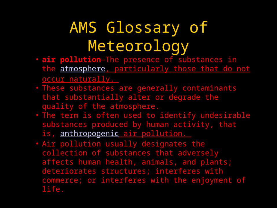
AMS Glossary of Meteorology• air pollution—The presence of substances in the
atmosphere, particularly those that do not occur naturally.
• These substances are generally contaminants that substantially alter or degrade the quality of the atmosphere.
• The term is often used to identify undesirable substances produced by human activity, that is, anthropogenic air pollution.
• Air pollution usually designates the collection of substances that adversely affects human health, animals, and plants; deteriorates structures; interferes with commerce; or interferes with the enjoyment of life.
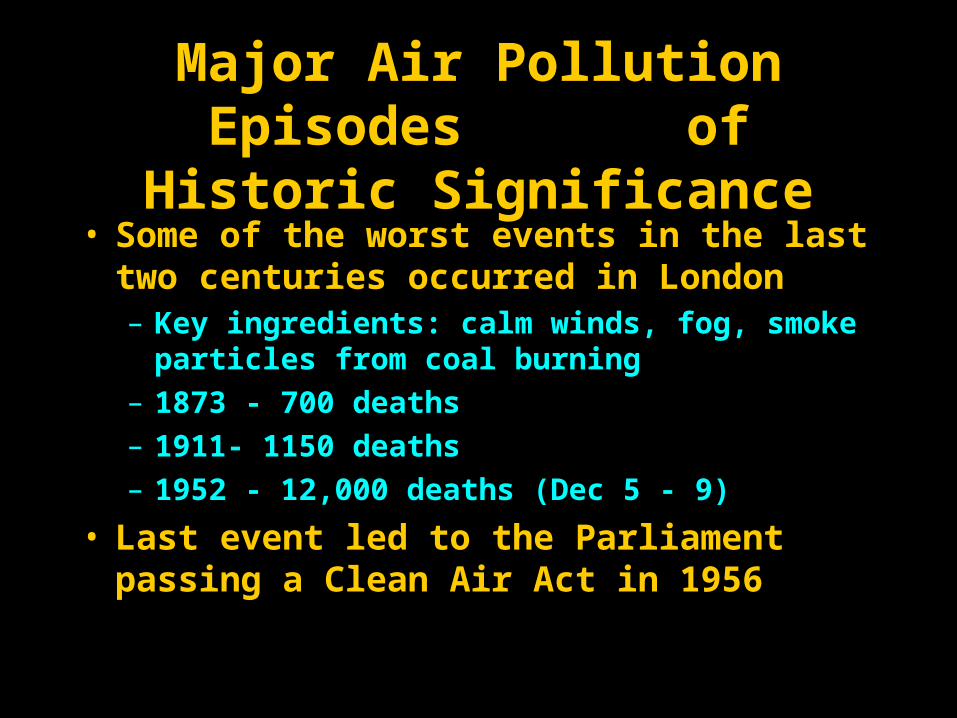
Major Air Pollution Episodes of Historic Significance
• Some of the worst events in the last two centuries occurred in London – Key ingredients: calm winds, fog, smoke particles
from coal burning
– 1873 - 700 deaths
– 1911- 1150 deaths
– 1952 - 12,000 deaths (Dec 5 - 9)
• Last event led to the Parliament passing a Clean Air Act in 1956
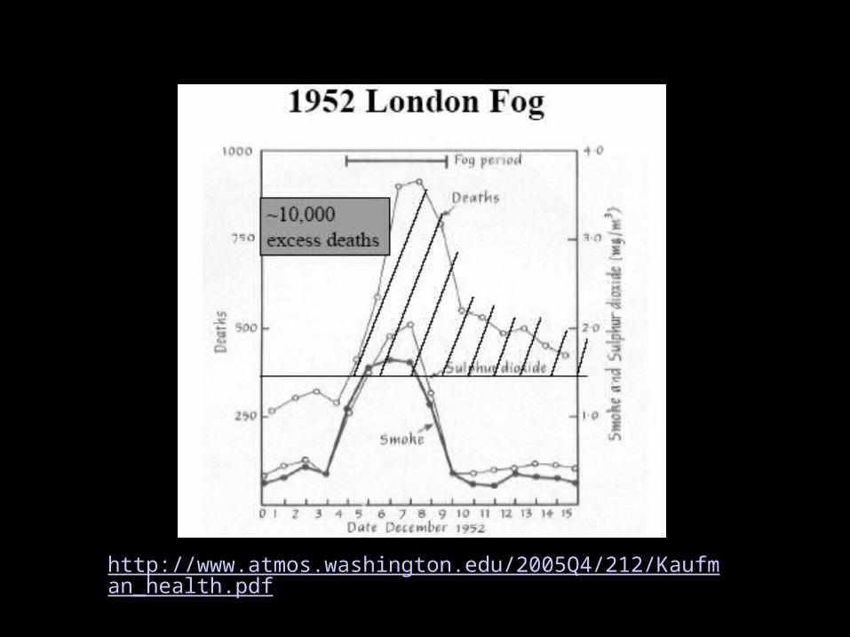
http://www.atmos.washington.edu/2005Q4/212/Kaufman_health.pdf

Major U.S. Air Pollution Episodes of Historic Significance
• U.S. air quality degraded shortly after the beginning of the industrial revolution
• Coal burning in Central and Midwest U.S. – 1939 St. Louis Smog Nov 28
– 1948 Donora, PA in the Monongahela River Valley
– 20 deaths, 1000’s took ill in 5 days Oct 27
• Prompted Air Pollution Control Act of 1955– Ignored automobiles

Major U.S. Air Pollution Episodes of Historic Significance
• 1960s - NYC had several severe smog episodes • 1950s onward – LA had many smog alerts from
an increase in industry and motor vehicle use• Led to passage of the Clean Air Act of 1970
(updated 1977 and 1990) – Empowered Federal Government to set emission
standards that each state had to meet
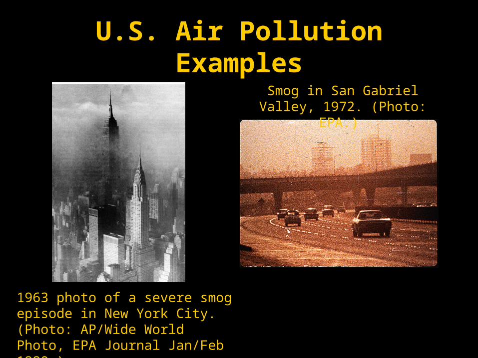
U.S. Air Pollution Examples
1963 photo of a severe smog episode in New York City. (Photo: AP/Wide World Photo, EPA Journal Jan/Feb 1990.)
Smog in San Gabriel Valley, 1972. (Photo: EPA.)
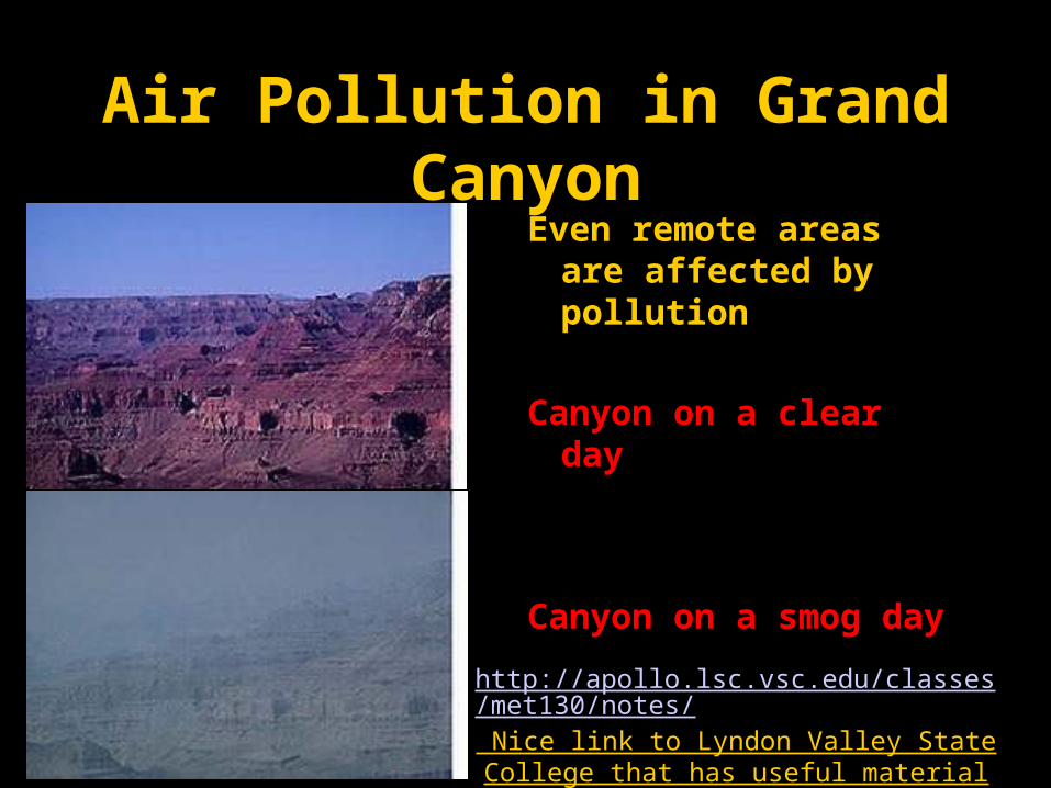
Air Pollution in Grand CanyonEven remote areas are
affected by pollution
Canyon on a clear day
Canyon on a smog day
http://apollo.lsc.vsc.edu/classes/met130/notes/ Nice link to Lyndon Valley State College that has useful material for a NATS-type course
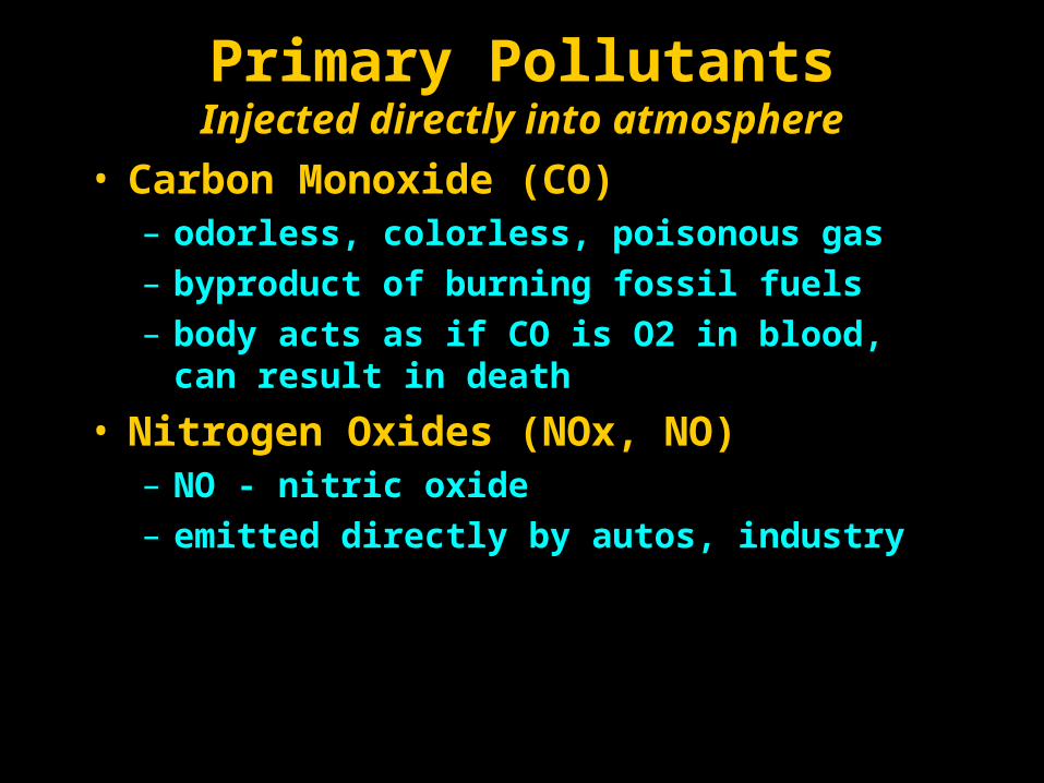
Primary PollutantsInjected directly into atmosphere
• Carbon Monoxide (CO) – odorless, colorless, poisonous gas
– byproduct of burning fossil fuels
– body acts as if CO is O2 in blood, can result in death
• Nitrogen Oxides (NOx, NO) – NO - nitric oxide
– emitted directly by autos, industry
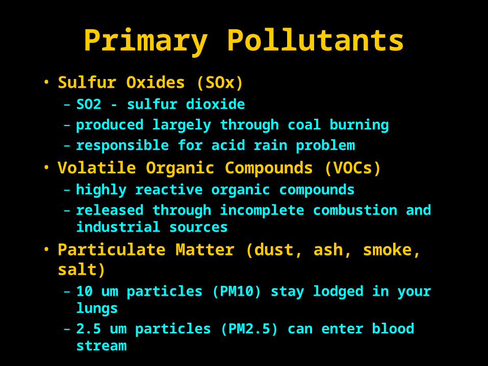
Primary Pollutants• Sulfur Oxides (SOx)
– SO2 - sulfur dioxide
– produced largely through coal burning
– responsible for acid rain problem
• Volatile Organic Compounds (VOCs) – highly reactive organic compounds
– released through incomplete combustion and industrial sources
• Particulate Matter (dust, ash, smoke, salt) – 10 um particles (PM10) stay lodged in your lungs
– 2.5 um particles (PM2.5) can enter blood stream
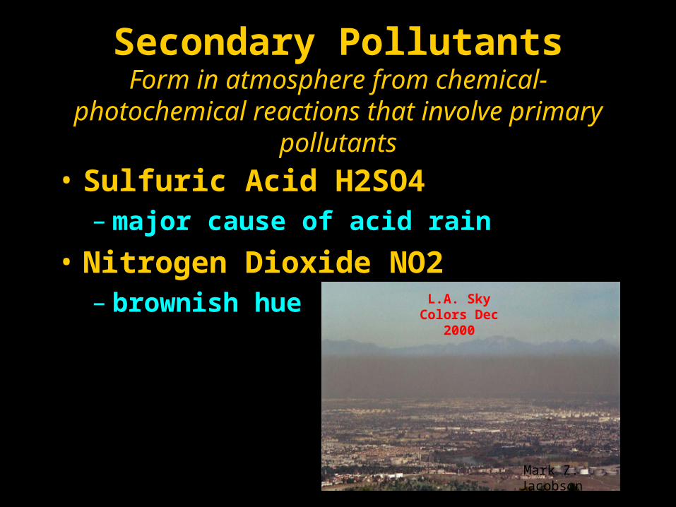
Secondary PollutantsForm in atmosphere from chemical-photochemical
reactions that involve primary pollutants
• Sulfuric Acid H2SO4 – major cause of acid rain
• Nitrogen Dioxide NO2 – brownish hue L.A. Sky Colors
Dec 2000
Mark Z. Jacobson
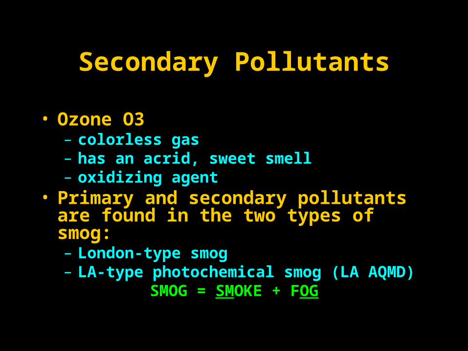
Secondary Pollutants
• Ozone O3 – colorless gas – has an acrid, sweet smell – oxidizing agent
• Primary and secondary pollutants are found in the two types of smog: – London-type smog – LA-type photochemical smog (LA AQMD)
SMOG = SMOKE + FOG
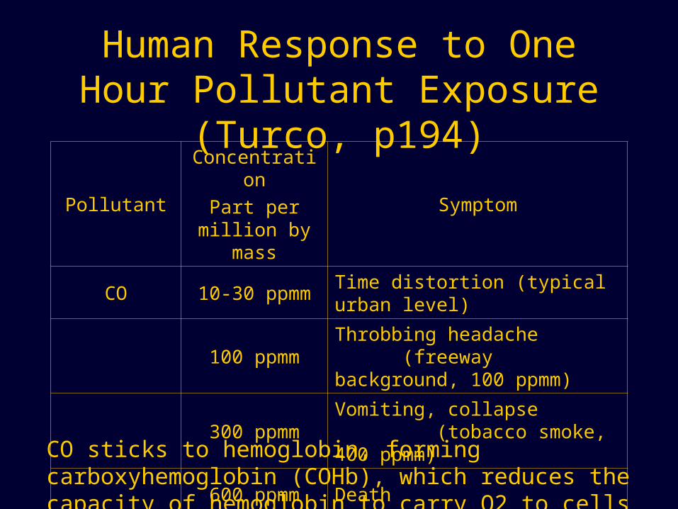
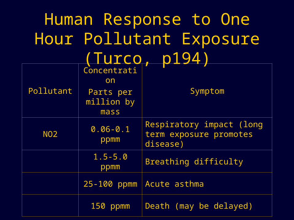
Human Response to One Hour Pollutant Exposure (Turco, p194)
PollutantConcentration
Part per million by mass
Symptom
CO 10-30 ppmm Time distortion (typical urban level)
100 ppmmThrobbing headache (freeway background, 100 ppmm)
300 ppmmVomiting, collapse (tobacco smoke, 400 ppmm)
600 ppmm Death
CO sticks to hemoglobin, forming carboxyhemoglobin (COHb), which reduces the capacity of hemoglobin to carry O2 to cells
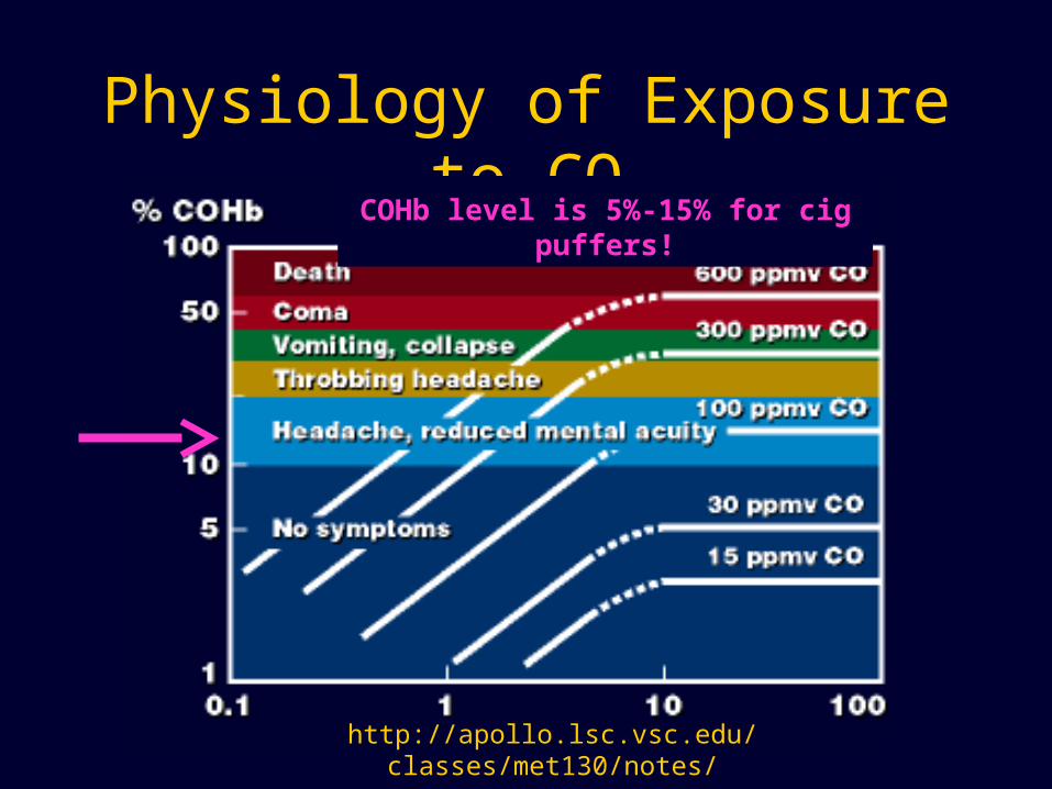
Physiology of Exposure to CO
http://apollo.lsc.vsc.edu/classes/met130/notes/
COHb level is 5%-15% for cig puffers!
Human Response to One Hour Pollutant Exposure (Turco, p194)
PollutantConcentration
Parts per million by mass
Symptom
NO2 0.06-0.1 ppmmRespiratory impact (long term exposure promotes disease)
1.5-5.0 ppmm Breathing difficulty
25-100 ppmm Acute asthma
150 ppmm Death (may be delayed)
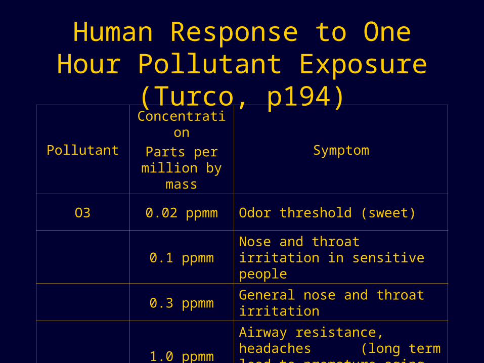
Human Response to One Hour Pollutant Exposure (Turco, p194)
PollutantConcentration
Parts per million by mass
Symptom
O3 0.02 ppmm Odor threshold (sweet)
0.1 ppmmNose and throat irritation in sensitive people
0.3 ppmm General nose and throat irritation
1.0 ppmmAirway resistance, headaches (long term lead to premature aging of lung tissue)

Human Response to One Hour Pollutant Exposure (Turco, p194)
PollutantConcentration
Parts per million by mass
Symptom
SO2 0.3 ppmm Taste threshold (acidic)
0.5 ppmm Odor threshold (acrid)
1.5 ppmmBronchiolar constriction Respiratory infection
Table 12-2, p.328
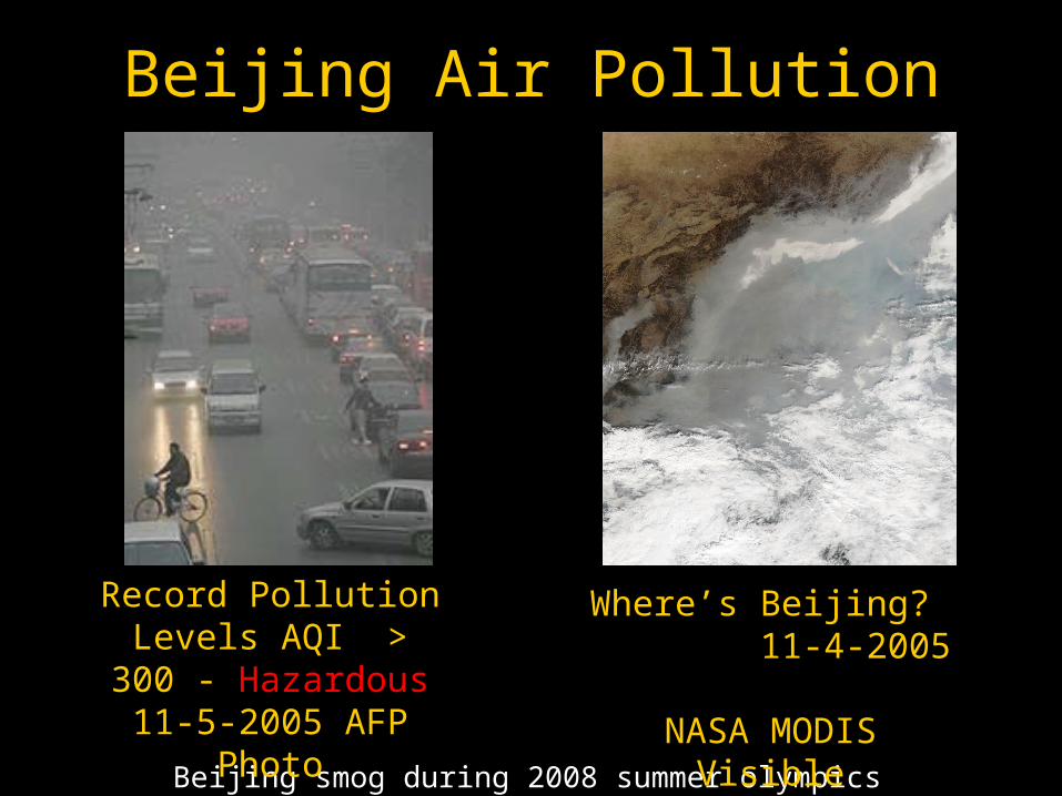
Beijing Air Pollution
http://www.terradaily.com/news/pollution-05zs.html
Beijing smog during 2008 summer olympics
Record Pollution Levels AQI > 300 - Hazardous 11-5-2005 AFP Photo
Where’s Beijing? 11-4-2005
NASA MODIS Visible
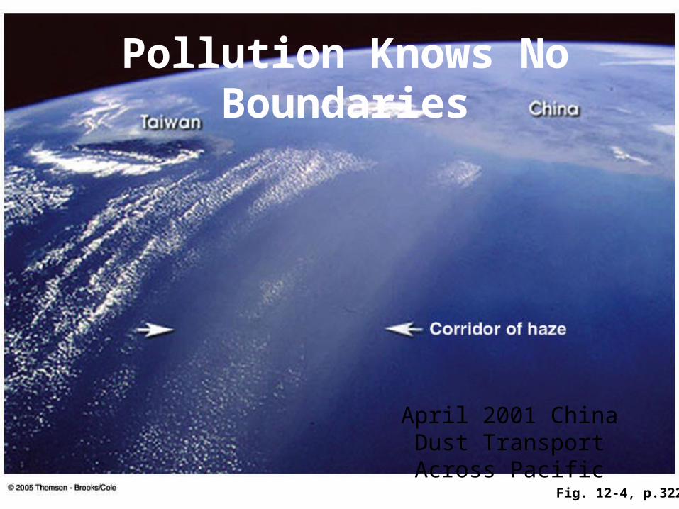
Fig. 12-4, p.322
Pollution Knows No Boundaries
April 2001 China Dust Transport Across Pacific
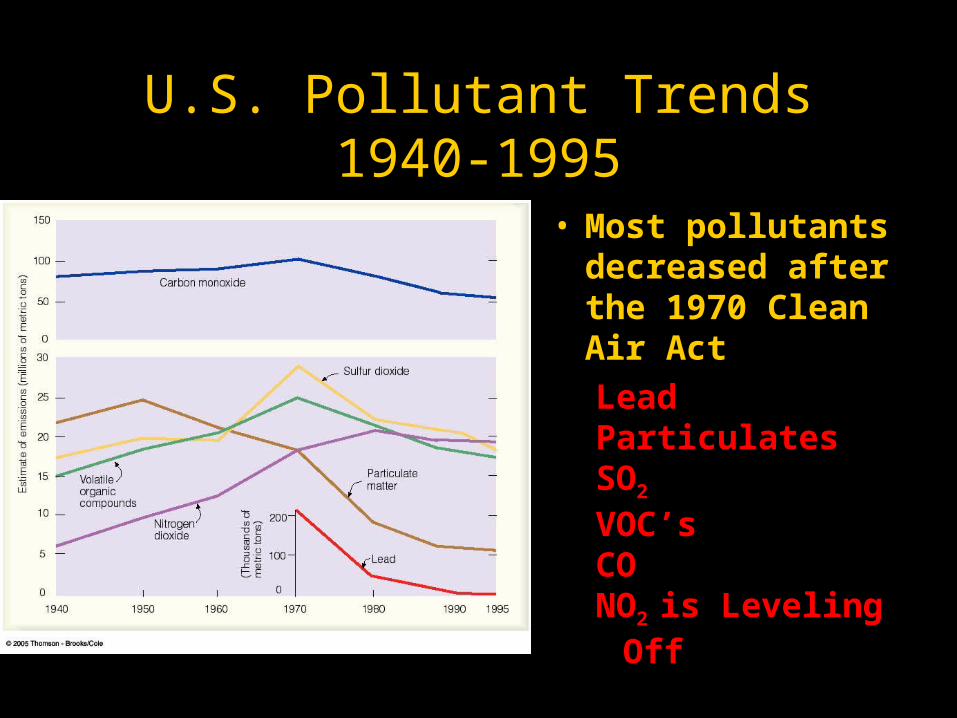
U.S. Pollutant Trends1940-1995
• Most pollutants decreased after the 1970 Clean Air Act
LeadParticulates SO2
VOC’sCONO2 is Leveling Off
Fig. 12-9, p.328
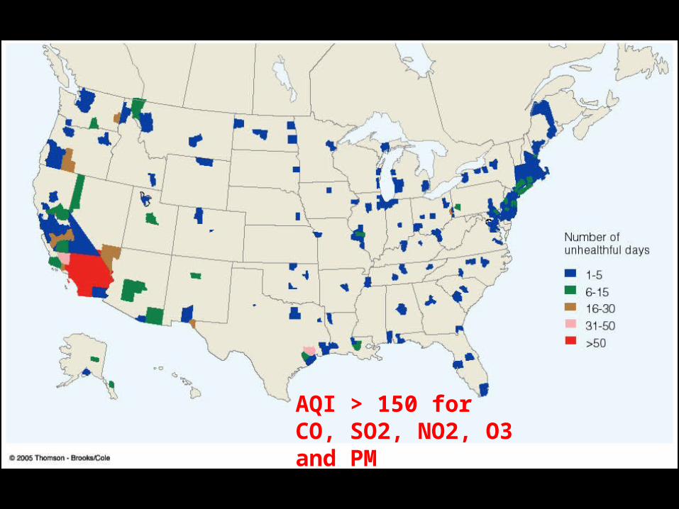
Fig. 12-10, p.329
AQI > 150 for CO, SO2, NO2, O3 and PM
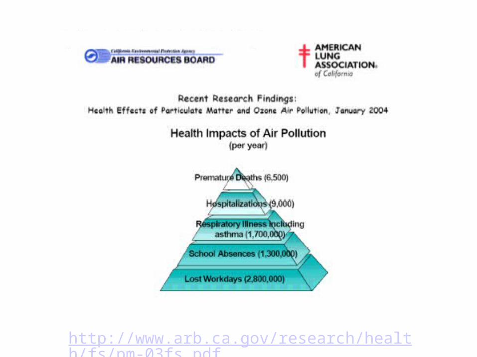
http://www.arb.ca.gov/research/health/fs/pm-03fs.pdf
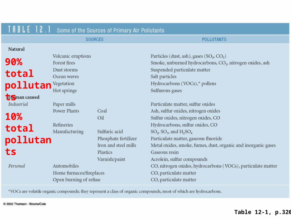
Table 12-1, p.320
90% total pollutants
10% total pollutants
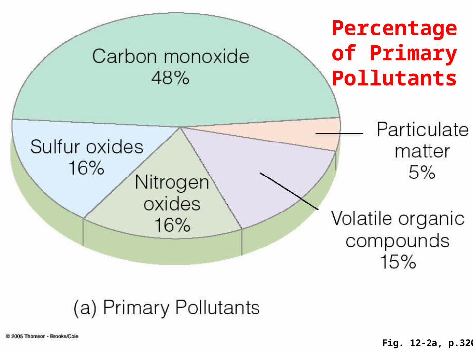
Fig. 12-2a, p.320
Percentage of Primary
Pollutants

Fig. 12-2b, p.320
Percentage of Primary Sources
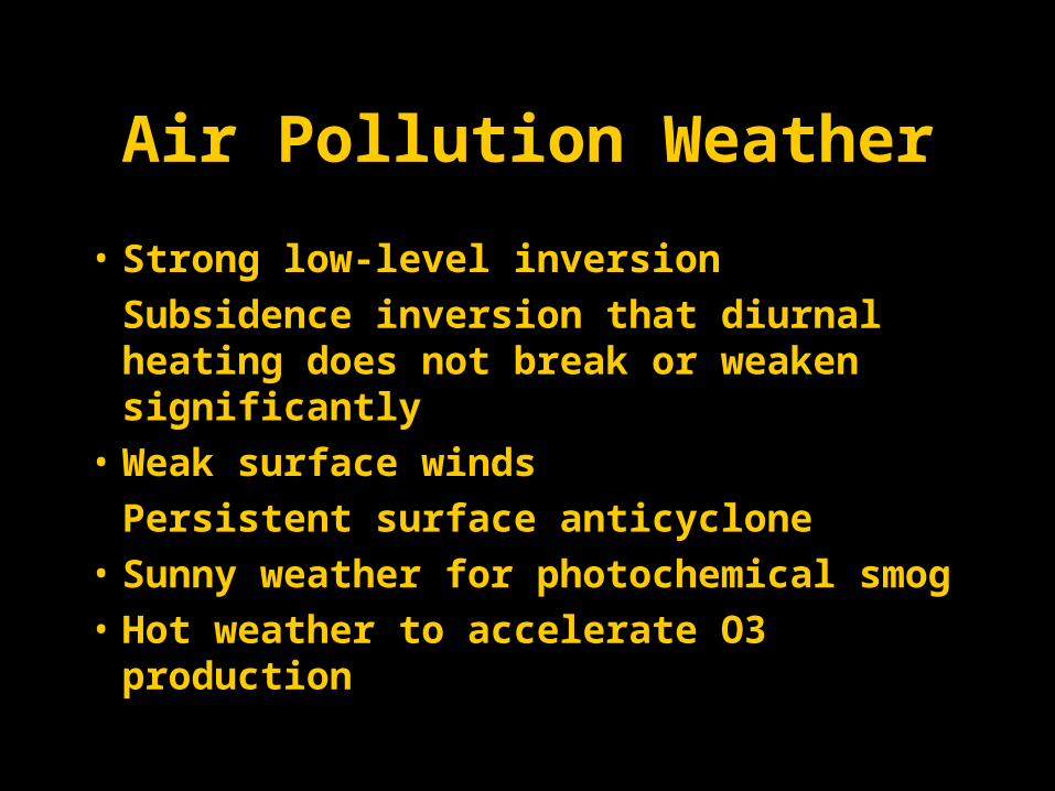
Air Pollution Weather
• Strong low-level inversion
Subsidence inversion that diurnal heating does not break or weaken significantly
• Weak surface winds
Persistent surface anticyclone
• Sunny weather for photochemical smog
• Hot weather to accelerate O3 production
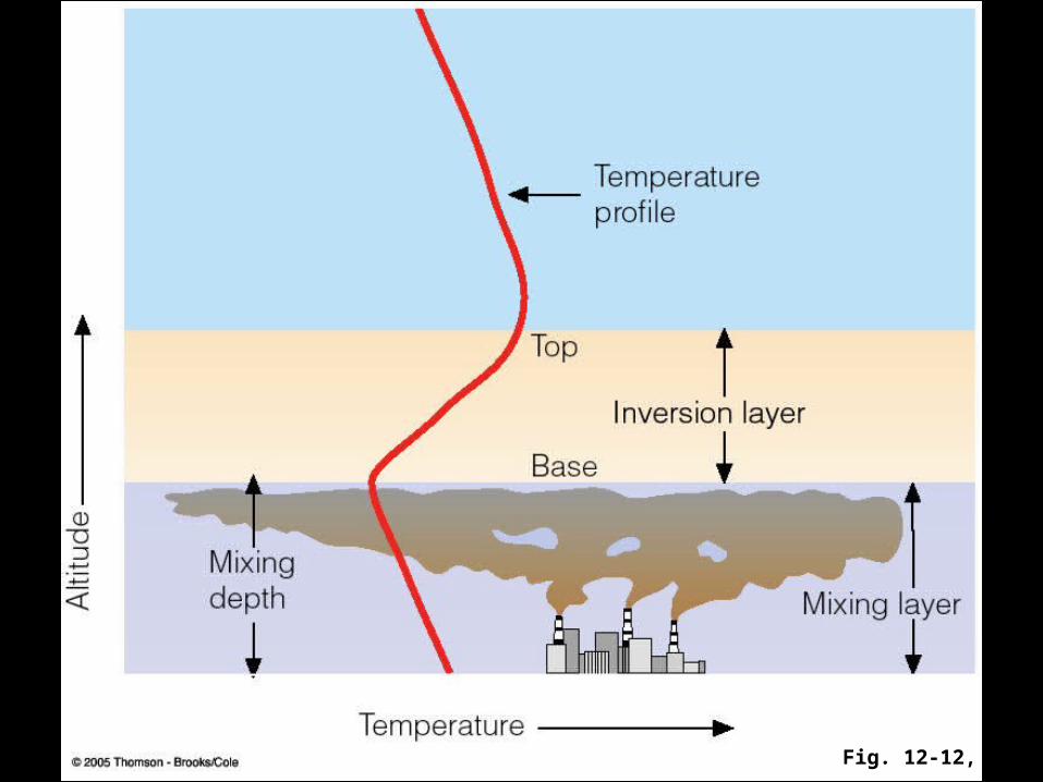
Fig. 12-12, p.333
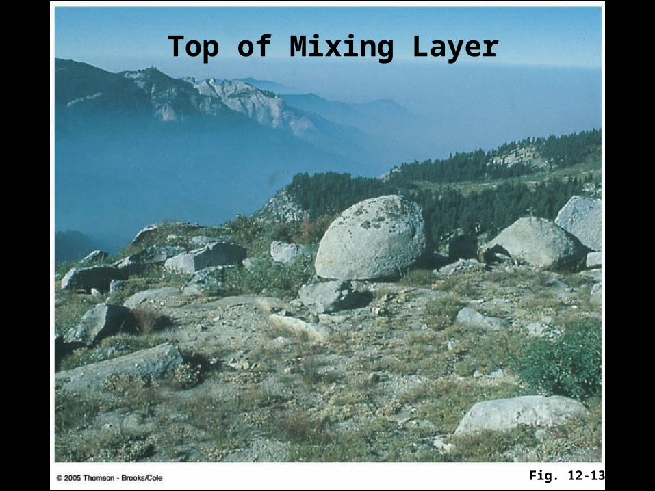
Fig. 12-13, p.333
Top of Mixing Layer
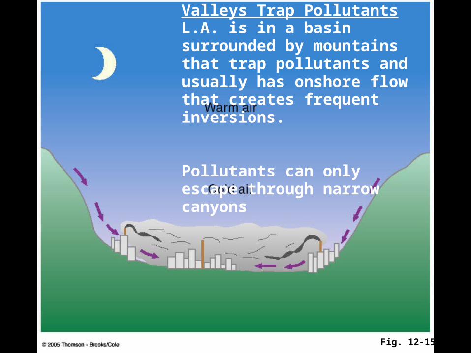
Fig. 12-15, p.334
Valleys Trap PollutantsL.A. is in a basin surrounded by mountains that trap pollutants and usually has onshore flow that creates frequent inversions.
Pollutants can only escape through narrow canyons
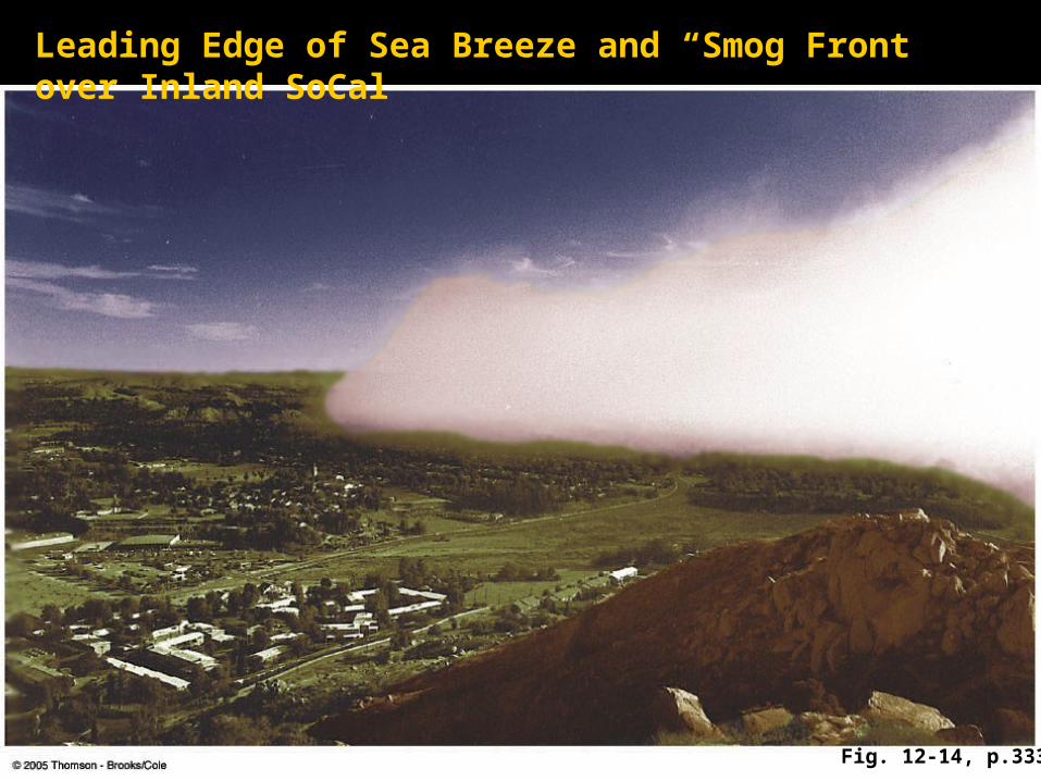
Fig. 12-14, p.333
Leading Edge of Sea Breeze and “Smog Front” over Inland SoCal
Air Pollution Dispersion
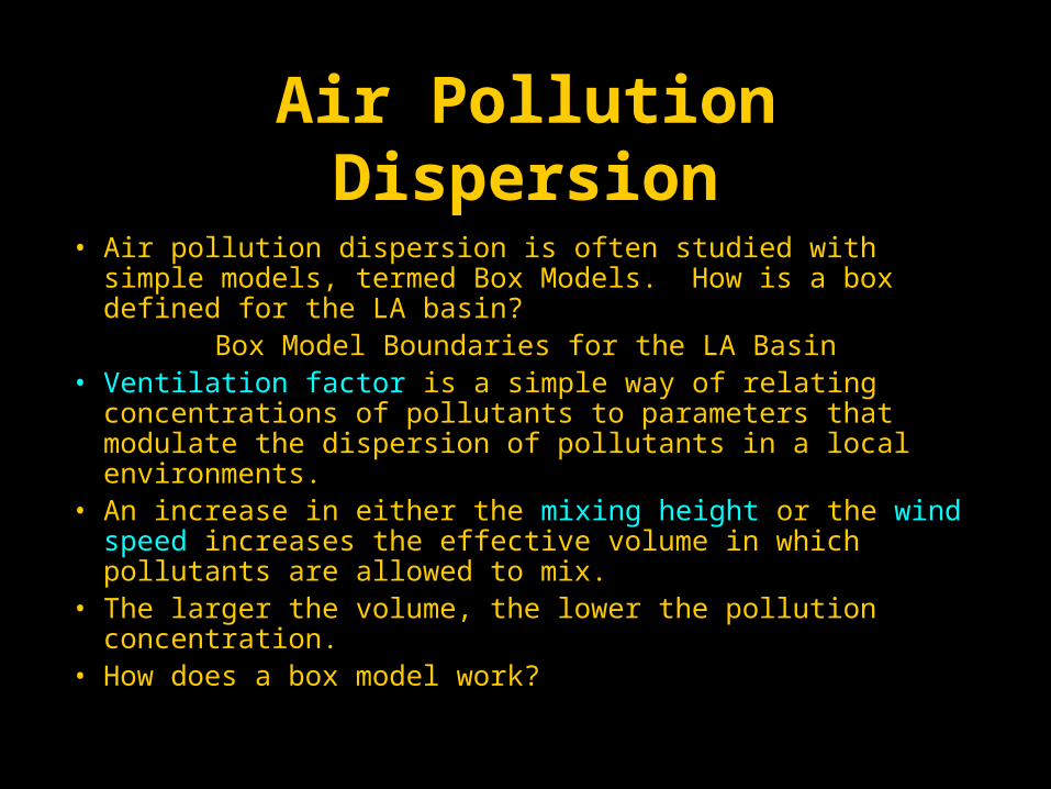
• Air pollution dispersion is often studied with simple models, termed Box Models. How is a box defined for the LA basin?
Box Model Boundaries for the LA Basin• Ventilation factor is a simple way of relating concentrations
of pollutants to parameters that modulate the dispersion of pollutants in a local environments.
• An increase in either the mixing height or the wind speed increases the effective volume in which pollutants are allowed to mix.
• The larger the volume, the lower the pollution concentration.• How does a box model work?
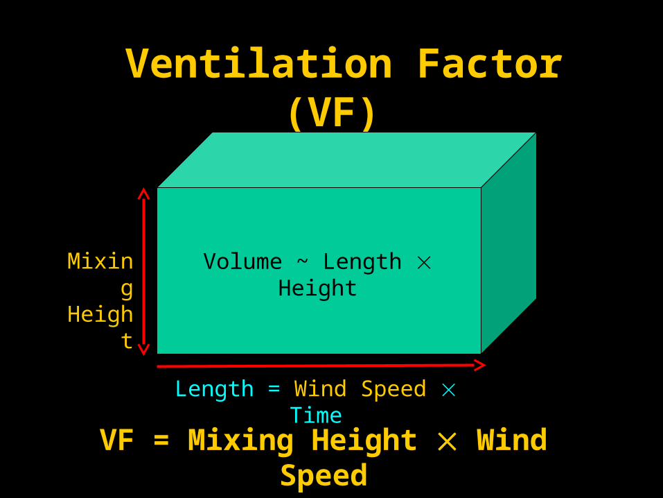
Ventilation Factor (VF)
Mixing Height
Length = Wind Speed Time
VF = Mixing Height Wind Speed
Volume ~ Length Height
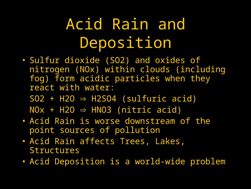
Acid Rain and Deposition
• Sulfur dioxide (SO2) and oxides of nitrogen (NOx) within clouds (including fog) form acidic particles when they react with water:
SO2 + H2O H2SO4 (sulfuric acid) NOx + H2O HNO3 (nitric acid)
• Acid Rain is worse downstream of the point sources of pollution
• Acid Rain affects Trees, Lakes, Structures• Acid Deposition is a world-wide problem
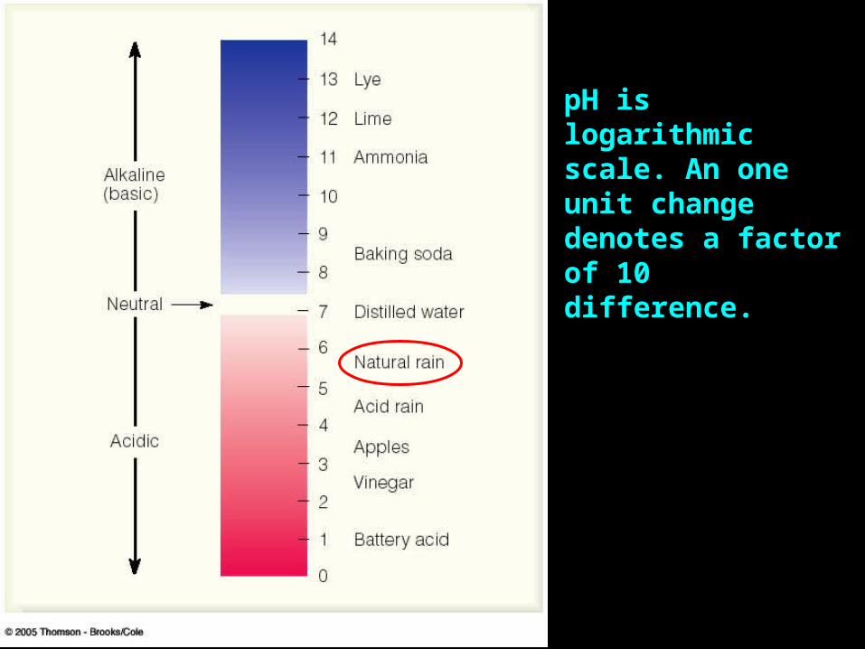
Fig. 12-17, p.338
pH is logarithmic scale. An one unit change denotes a factor of 10 difference.
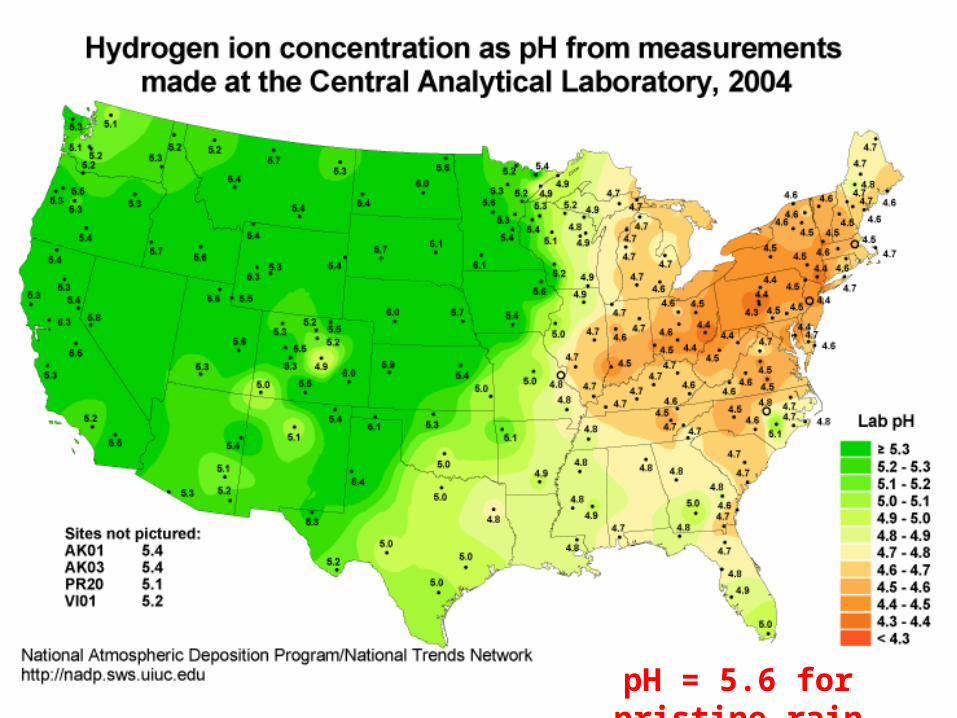
pH = 5.6 for pristine rain
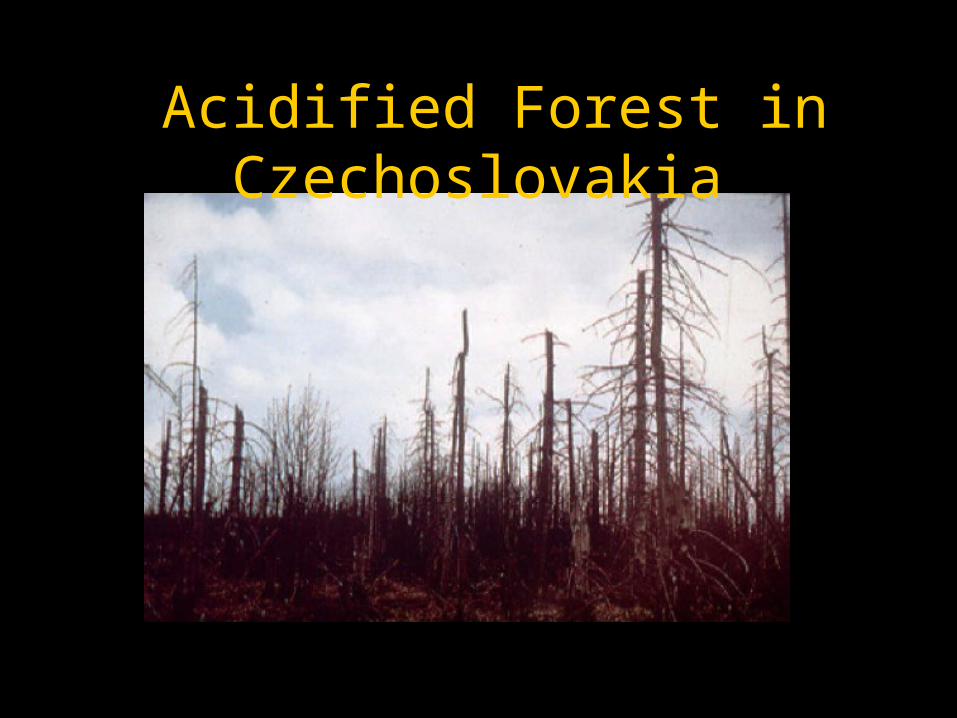
Fig. 12-19, p.339
Acidified Forest in Czechoslovakia
http://www.atmos.washington.edu/2005Q4/212/AcidDepositionSlides.pdf
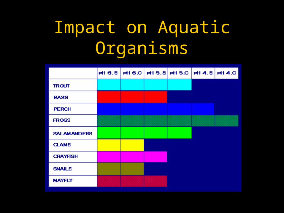
Impact on Aquatic Organisms
http://www.epa.gov/airmarkets/acidrain/effects/surfacewater.html#fish
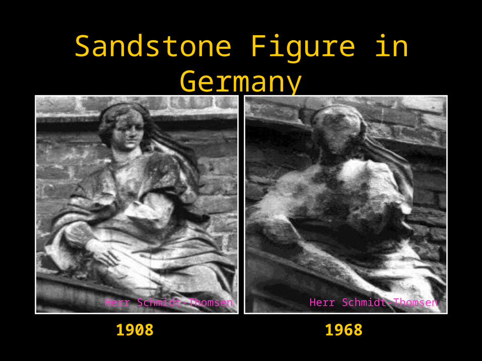
Sandstone Figure in Germany
1908 1968
Herr Schmidt-ThomsenHerr Schmidt-Thomsen
http://www.atmos.washington.edu/2005Q4/212/AcidDepositionSlides.pdf
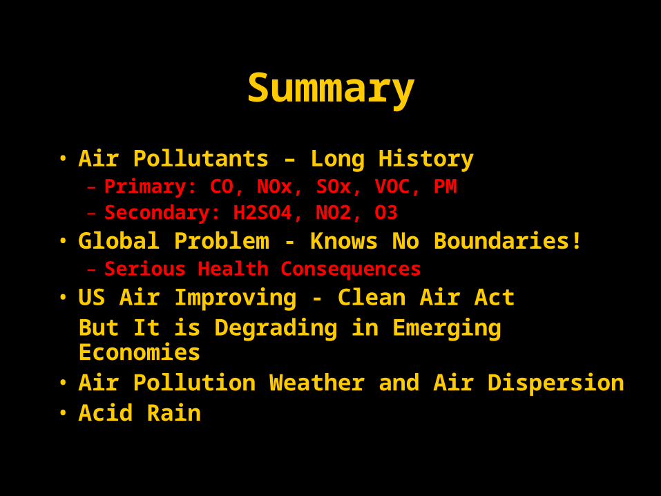
Summary
• Air Pollutants – Long History– Primary: CO, NOx, SOx, VOC, PM – Secondary: H2SO4, NO2, O3
• Global Problem - Knows No Boundaries!– Serious Health Consequences
• US Air Improving - Clean Air ActBut It is Degrading in Emerging Economies
• Air Pollution Weather and Air Dispersion• Acid Rain
NATS 101
Lecture Ozone Depletion
Supplemental References for Today’s Lecture
Danielson, E. W., J. Levin and E. Abrams, 1998: Meteorology. 462 pp. McGraw-Hill. (ISBN 0-697-21711-6)
Moran, J. M., and M. D. Morgan, 1997: Meteorology, The Atmosphere and the Science of Weather, 5th Ed. 530 pp. Prentice Hall. (ISBN 0-13-266701-0)
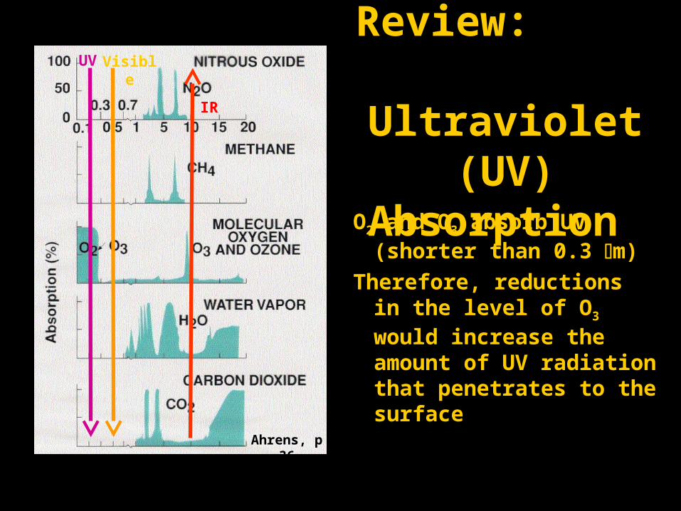
Review: Ultraviolet (UV)
Absorption O2 and O3 absorb UV
(shorter than 0.3 m)
Therefore, reductions in the level of O3 would increase the amount of UV radiation that penetrates to the surface
IR
Ahrens, p 36
UV Visible
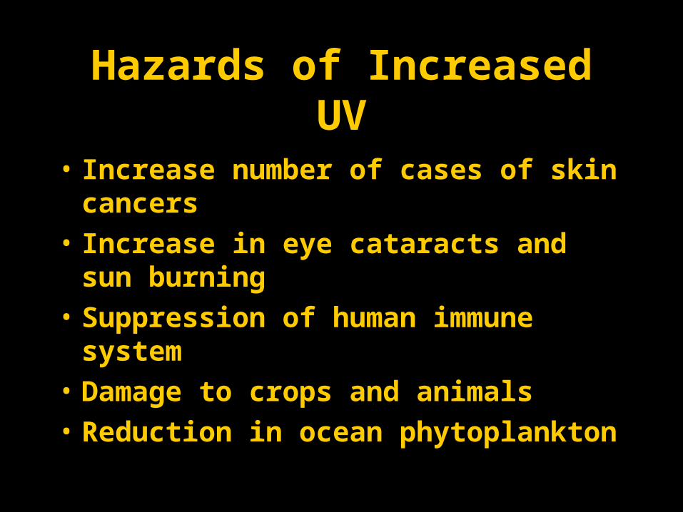
Hazards of Increased UV
• Increase number of cases of skin cancers
• Increase in eye cataracts and sun burning
• Suppression of human immune system
• Damage to crops and animals
• Reduction in ocean phytoplankton
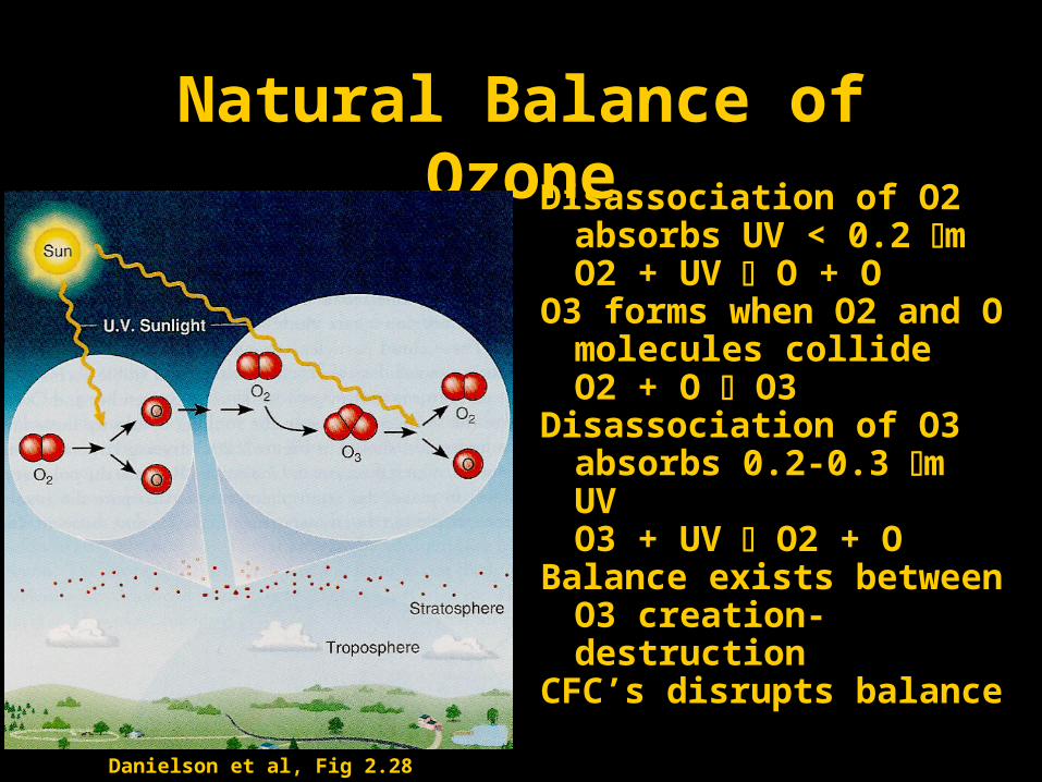
Natural Balance of Ozone
Danielson et al, Fig 2.28
Disassociation of O2 absorbs UV < 0.2 mO2 + UV O + O
O3 forms when O2 and O molecules collideO2 + O O3
Disassociation of O3 absorbs 0.2-0.3 m UVO3 + UV O2 + O
Balance exists between O3 creation-destruction
CFC’s disrupts balance
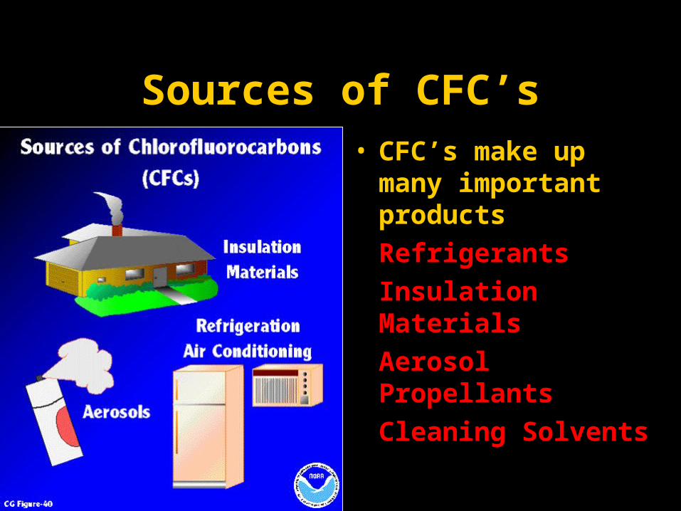
Sources of CFC’s• CFC’s make up many
important products
Refrigerants
Insulation Materials
Aerosol Propellants
Cleaning Solvents
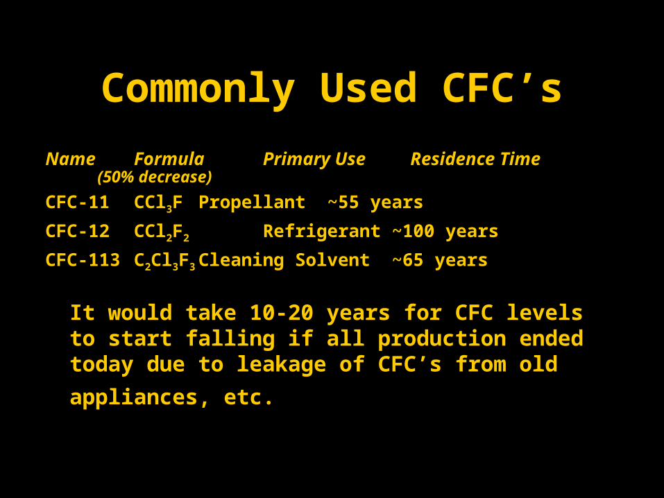
Commonly Used CFC’s
Name Formula Primary Use Residence Time (50% decrease)
CFC-11 CCl3F Propellant ~55 years
CFC-12 CCl2F2 Refrigerant ~100 years
CFC-113 C2Cl3F3 Cleaning Solvent ~65 years
It would take 10-20 years for CFC levels to start falling if all production ended today due to leakage of CFC’s from
old appliances, etc.
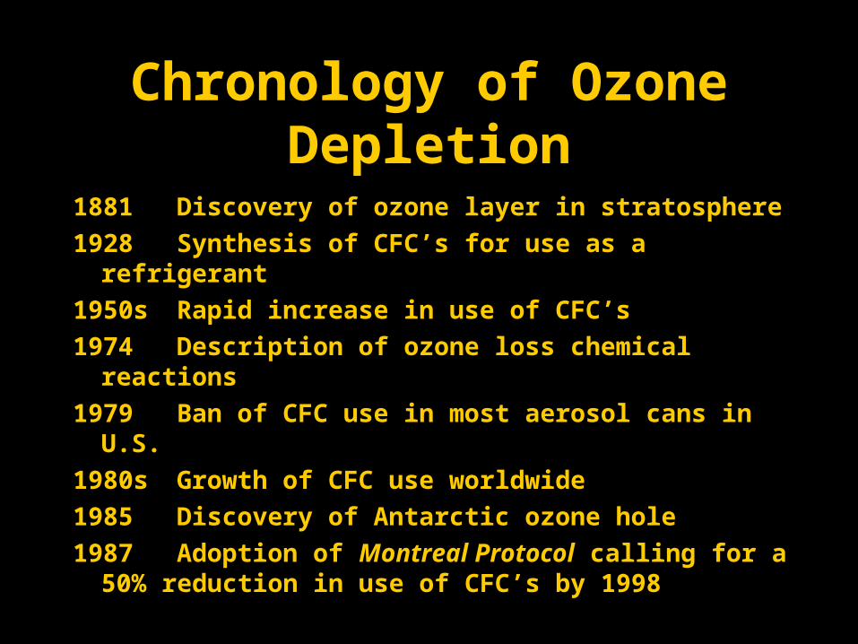
Chronology of Ozone Depletion
1881 Discovery of ozone layer in stratosphere
1928 Synthesis of CFC’s for use as a refrigerant
1950s Rapid increase in use of CFC’s
1974 Description of ozone loss chemical reactions
1979 Ban of CFC use in most aerosol cans in U.S.
1980s Growth of CFC use worldwide
1985 Discovery of Antarctic ozone hole
1987 Adoption of Montreal Protocol calling for a 50% reduction in use of CFC’s by 1998
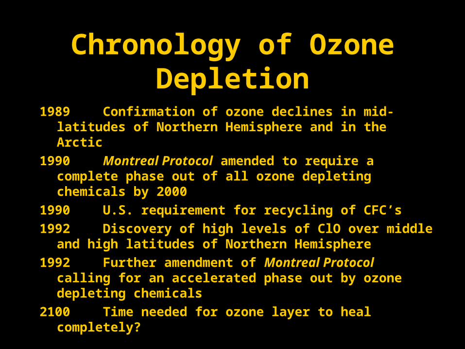
Chronology of Ozone Depletion
1989 Confirmation of ozone declines in mid-latitudes of Northern Hemisphere and in the Arctic
1990 Montreal Protocol amended to require a complete phase out of all ozone depleting chemicals by 2000
1990 U.S. requirement for recycling of CFC’s
1992 Discovery of high levels of ClO over middle and high latitudes of Northern Hemisphere
1992 Further amendment of Montreal Protocol calling for an accelerated phase out by ozone depleting chemicals
2100 Time needed for ozone layer to heal completely?

How O3 is Measured: Dobson Unit
• Ozone can be measured by the depth of ozone if all ozone in a column of atmosphere is brought to sea-level temperature and pressure.
• One Dobson unit corresponds to a 0.01 mm depth at sea-level temperature and pressure
• The ozone layer is very thin in Dobson units.
There are only a few millimeters (few hundred Dobsons) of total ozone in a column of air.
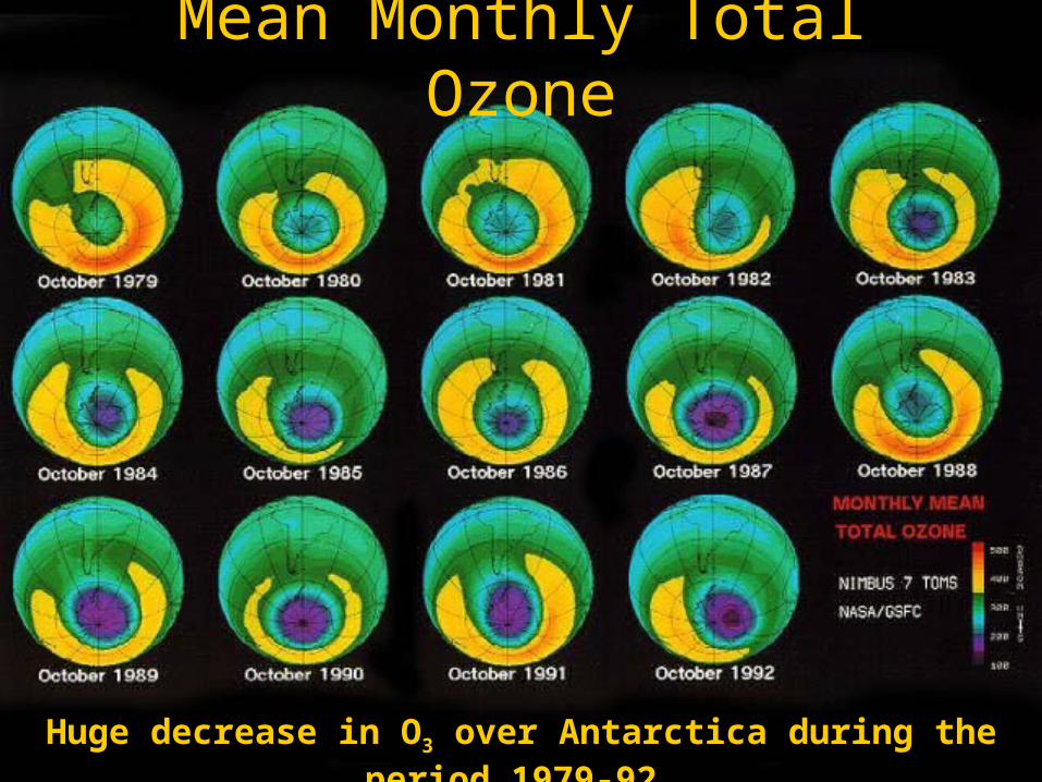
Mean Monthly Total Ozone
Huge decrease in O3 over Antarctica during the period 1979-92.
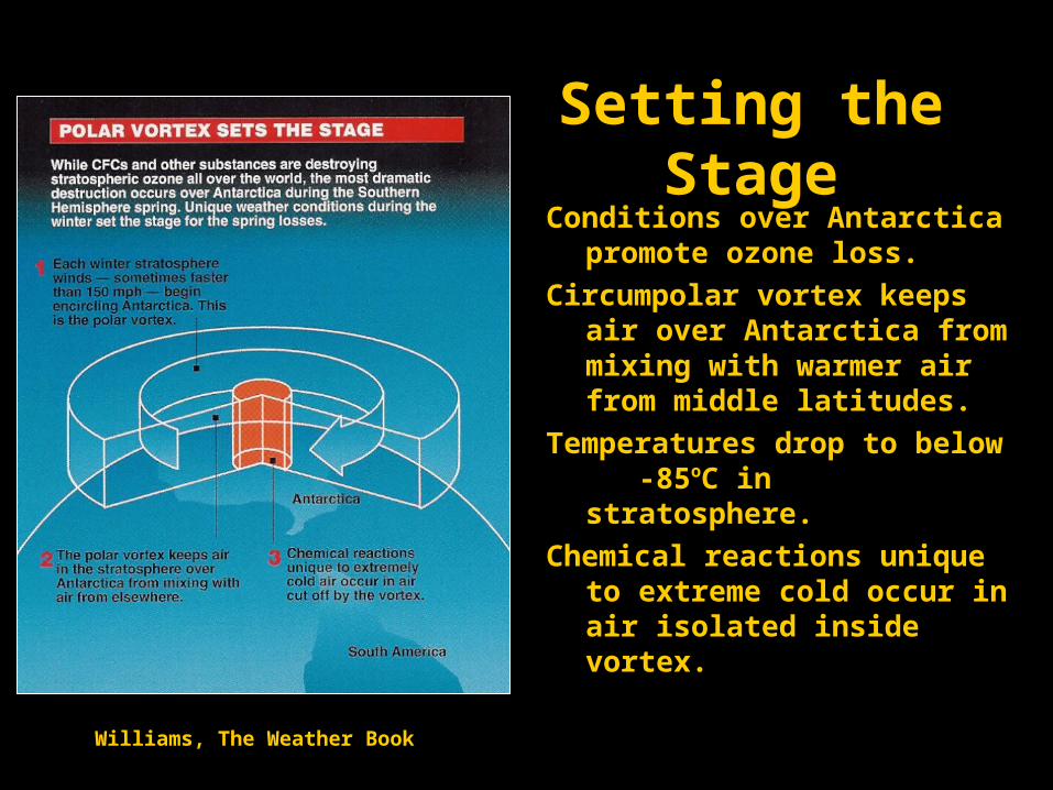
Setting the StageConditions over Antarctica promote
ozone loss.
Circumpolar vortex keeps air over Antarctica from mixing with warmer air from middle latitudes.
Temperatures drop to below -85oC in stratosphere.
Chemical reactions unique to extreme cold occur in air isolated inside vortex.
Williams, The Weather Book
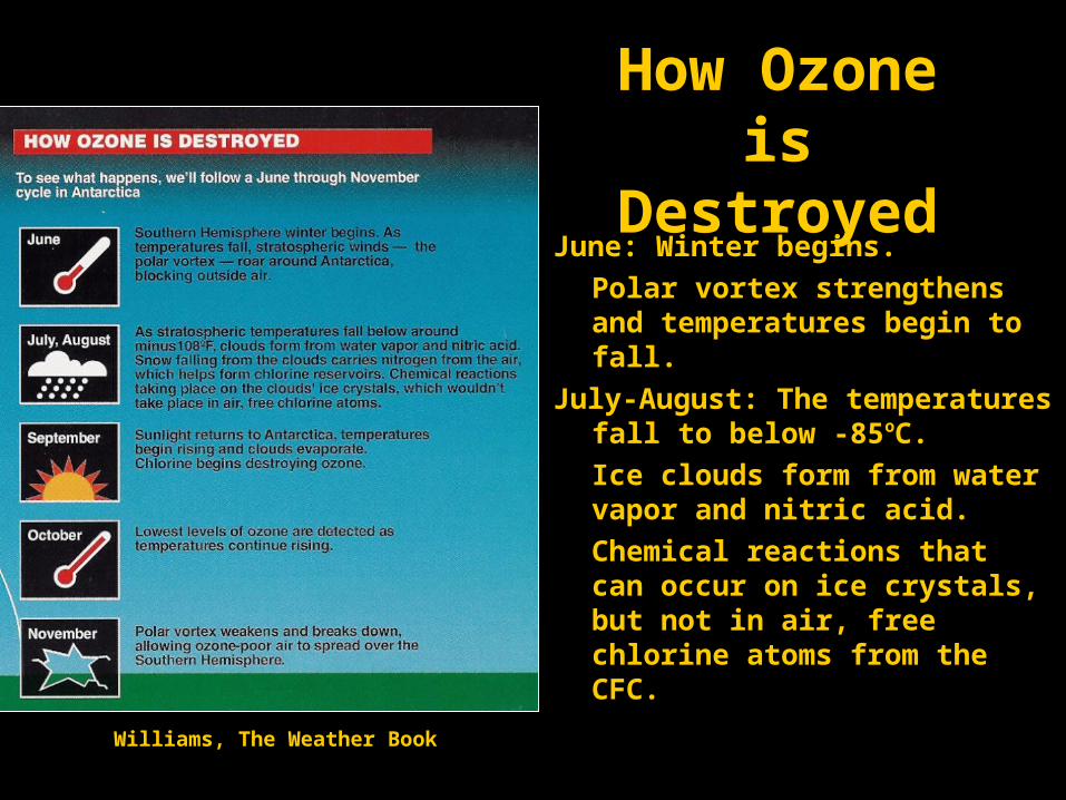
How Ozone is Destroyed
June: Winter begins.
Polar vortex strengthens and temperatures begin to fall.
July-August: The temperatures fall to below -85oC.
Ice clouds form from water vapor and nitric acid.
Chemical reactions that can occur on ice crystals, but not in air, free chlorine atoms from the CFC.
Williams, The Weather Book
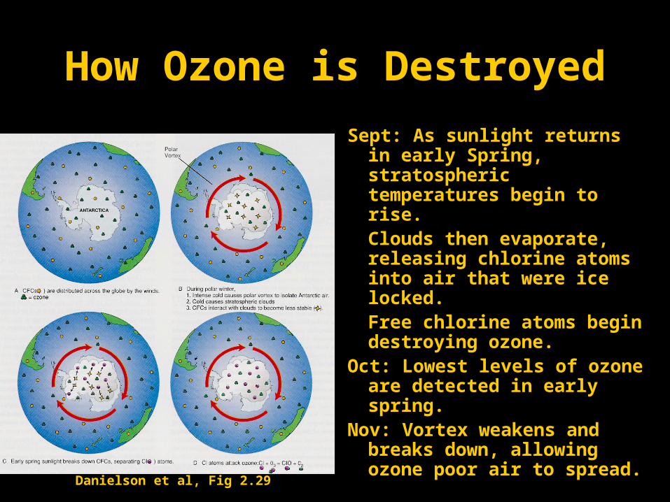
How Ozone is Destroyed
Sept: As sunlight returns in early Spring, stratospheric temperatures begin to rise. Clouds then evaporate, releasing chlorine atoms into air that were ice locked. Free chlorine atoms begin destroying ozone.
Oct: Lowest levels of ozone are detected in early spring.
Nov: Vortex weakens and breaks down, allowing ozone poor air to spread.
Danielson et al, Fig 2.29
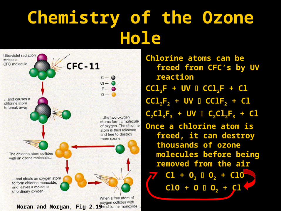
Chemistry of the Ozone Hole
Chlorine atoms can be freed from CFC’s by UV reaction
CCl3F + UV CCl2F + Cl
CCl2F2 + UV CClF2 + Cl
C2Cl3F3 + UV C2Cl2F3 + Cl
Once a chlorine atom is freed, it can destroy thousands of ozone molecules before being removed from the air
Cl + O3 O2 + ClO
ClO + O O2 + Cl
Moran and Morgan, Fig 2.19
CFC-11
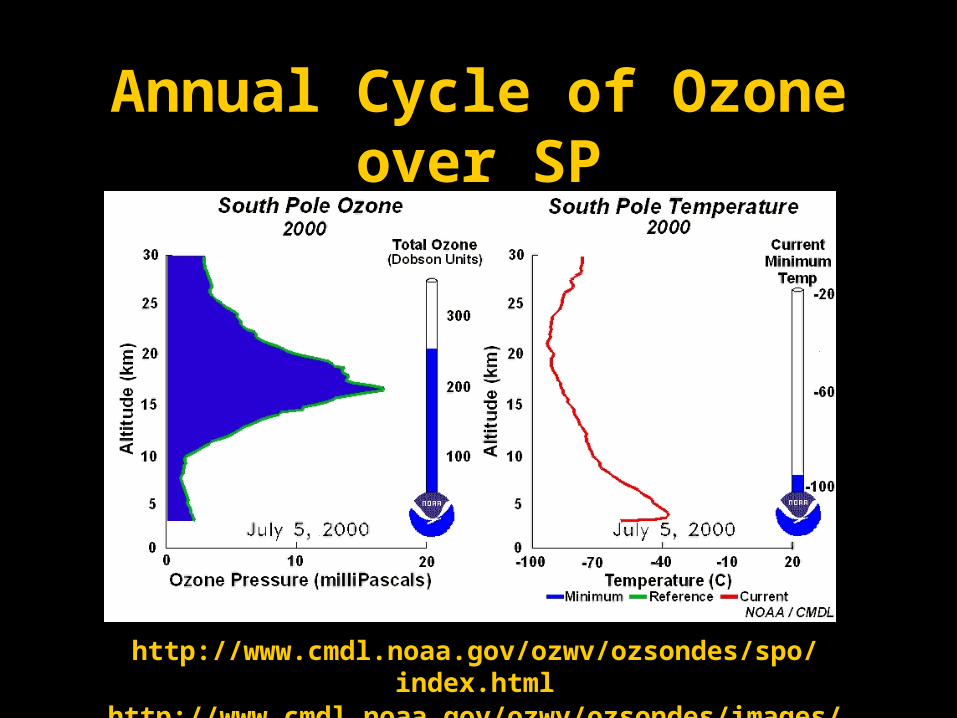
Annual Cycle of Ozone over SP
http://www.cmdl.noaa.gov/ozwv/ozsondes/spo/index.htmlhttp://www.cmdl.noaa.gov/ozwv/ozsondes/images/ozone_anim2001.avi
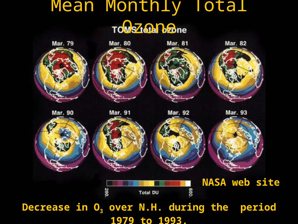
Mean Monthly Total Ozone
Decrease in O3 over N.H. during the period 1979 to 1993.
NASA web site
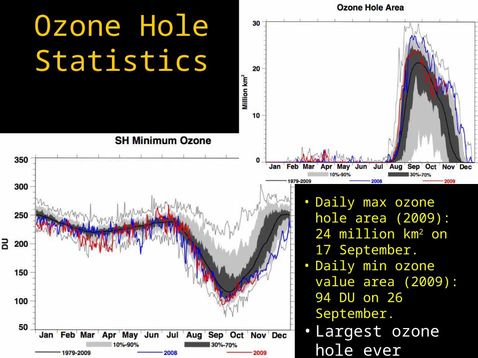
Ozone Hole Statistics
• Daily max ozone hole area (2009): 24 million km2 on 17 September.
• Daily min ozone value area (2009): 94 DU on 26 September.
• Largest ozone hole ever observed: 24 Sept 2006.
Key Points: Ozone Hole
• Chlorofluorocarbons (CFCs) disrupt the natural balance of O3 in S.H. stratosphere
CFCs responsible for the ozone hole over SP!
Responsible for lesser reductions worldwide.
• Special conditions exist in stratosphere over Antarctica that promote ozone destruction:
Air trapped inside circumpolar vortex
Cold temperatures fall to below -85oC
Key Points: Ozone Hole
• CFCs stay in atmosphere for ~100 years
One freed chlorine atom destroys thousands of O3 molecules before leaving stratosphere
• Montreal Protocol mandated total phase out of ozone depleting substances by 2000.
• Even with a complete phase out, O3 levels
Would not increase for another 10-20 years
Would not completely recover for ~100 years