NATIONALOPTICALASTRONOMYOBSERVATORIES

PreprintSeries

NOAOPreprintNo. 815

Standard Giant Branches in the Washington Photometric System

DougGeisler

Ata Sarajedini

To be publishedin: AstronomicalJournal,

January1999

October1998

Operatedfor the NationalScienceFoundationbythe Associationof Universitiesfor ResearchinAstronomy,Inc.

https://ntrs.nasa.gov/search.jsp?R=19990046718 2018-08-31T17:10:56+00:00Z

Standard Giant Branches in the Washington Photometric

System

Doug Geisler 1

Kitt Peak National Observatory, National Optical Astronomy Observatories,

P.O. Box 26732, Tucson, Arizona 85726

dgeisler@noao, edu

and

Ata Sarajedini 2

San Francisco State University, Dept. of Physics and Astronomy,

1600 Holloway Ave., San Francisco, CA 94132

ata@stars.sfsu, edu

Received ; accepted

astro-ph/9809393; to be published in January 1999 AJ

1Visiting Astronomer, Canada-France-Hawaii Telescope, operated by the National

Research Council of Canada, le Centre National de la Recherche Scientifique de France,

and the University of Hawaii.

2Hubble Fellow

-2-

ABSTRACT

We have obtained CCD photometry in the Washington system C, T1 filters

for some 850,000 objects associated with 10 Galactic globular clusters and 2 old

open clusters. These clusters have well-known metal abundances, spanning a

metallicity range of 2.5 dex from [Fe/H] _ -2.25 to +0.25 at a spacing of ,-_ 0.2

dex. Two independent observations were obtained for each cluster and internal

checks, as well as external comparisons with existing photoelectric photometry

, indicate that the final colors and magnitudes have overall uncertainties of <_

0.03 mag.

Analogous to the method employed by Da Costa and Armandroff (1990, A J,

100, 162) for V, I photometry , we then proceed to construct standard ( _-fw_

, (C - T1)0 ) giant branches for these clusters adopting the Lee et al. (1990,

ApJ, 350, 155) distance scale, using some 350 stars per globular cluster to

define the giant branch. We then determine the metallicity sensitivity of the

(C - T1)0 color at a given _IT, value. The Washington system technique

is found to have three times the metallicity sensitivity of the V, I technique.

At ]ICT_ = --2 (about a magnitude below the tip of the giant branch, roughly

equivalent to M1 = -3), the giant branches of 47 Tuc and M15 are separated by

1.16 magnitudes in (C - T1)0 and only 0.38 magnitudes in (V - I)0 • Thus,

for a given photometric accuracy, metallicities can be determined three times

more precisely with the Washington technique. We find a linear relationship

between (C- T1)0 (at MT, = --2) and metallicity (on the Zinn 1985, ApJ,

293, 424 scale) exists over the full metallicity range, with an rms of only 0.04

dex. We also derive metallicity calibrations for MT, ---- -2.5 and -1.5, as well

as for two other metallicity scales. The Washington technique retains almost

the same metallicity sensitivity at faint magnitudes, and indeed the standard

3

giant branches are still well separated even below the horizontal branch. The

photometry is used to set upper limits in the range 0.03 - 0.09 dex for any

intrinsic metallicity dispersion in the calibrating clusters. The calibrations are

applicable to objects with ages > 5 Gyr - any age effects are small or negligible

for such objects.

This new technique is found to have many advantages over the old two-color

diagram technique for deriving metallicities from Washington photometry

In addition to only requiring 2 filters instead of 3 or 4, the new technique

is generally much less sensitive to reddening and photometric errors, and the

metallicity sensitivity is many times higher. The new technique is especially

advantageous for metal-poor objects. The five metal-poor clusters determined

by Geisler et al. (1992, A J, 104, 627), using the old technique, to be much

more metal-poor than previous indications, yield metallicities using the

new technique which are in excellent agreement with the Zinn scale. The

anomalously low metallicities derived previously are undoubtedly a result of

the reduced metallicity sensitivity of the old technique at low abundance.

However, the old technique is still competitive for metal-rich objects ( [Fe/H]

> -1)

We have extended the method developed by Sarajedini (1994, AJ, 107, 618)

to derive simultaneous reddening and metallicity determinations from the

shape of the red giant branch, the T1 magnitude of the horizontal branch,

and the apparent (C - T1) color of the red giant branch at the level of the

horizontal branch. This technique allows us to measure reddening to 0.025

magnitudes in E(B - V) and metallicity to 0.15 dex. Reddenings can also be

derived from the blue edge of the instability strip, with a similar error.

\Ve measure the apparent T1 magnitude of the red giant branch bump

-4-

in each of the calibrating clusters and find that the difference in magnitude

between the bump and the horizontal branch is tightly and sensitively correlated

with metallicity, with an rms dispersion of 0.1 dex. This feature can therefore

also be used to derive metallicity in suitable objects. Metallicity can be

determined as well from the slope of the RGB, to a similar accuracy. Our very

populous color- magnitude diagrams reveal the asymptotic giant branch bump

in several clusters.

Although MT_ of the red giant branch tip is not as constant with

metallicity and age as Mi , it is still found to be a useful distance indicator

for objects with [Fe/H] < -1.2. For the 6 standard clusters in this regime,

< MT, (TRGB) >= -3.22 =t=0.11(a), with only a small metallicity dependence.

This result is found to be in very good agreement with the predictions of

the Bertelli et al. (1994, A&:AS, 106, 275) isochrones. We also note that the

Washington system holds great potential for deriving accurate ages as well as

metallicities.

Subject headings: Galaxy: abundances -- globular clusters: general

-5-

1. INTRODUCTION

The color of the first ascent, red giant branch (RGB) of an old stellar system has long

been recognized as a sensitive indicator of metal abundance (e.g. Sandage and Smith 1966,

Hartwick 1968, Rood 1978, Frogel et al. 1983). Observationally, the utility of this feature

for determining metallicity was first exploited using the traditional Johnson BV filters

by Hartwick (1968) in his definition of the (B - V)o,9 feature: the reddening -corrected

color of the RGB at the level of the horizontal branch (HB). Searle and Zinn (1978) formed

an abundance ranking from plots of My vs. a reddening-independent color derived from

spectral scans of globular cluster (GC) giants.

Da Costa and Armandroff (1990, hereafter DCA) extended this technique to the

V,/(Cousins) photometric system, quoting a large color baseline as one of their motivators.

They utilized the entire upper RGB, establishing standard GC giant branches in the (

MI , (V - I)0 ) plane. They demonstrated the substantial metallicity sensitivity of

the (V - I)0 color at a given M1 • This method now enjoys great popularity as the

preferred technique for, e.g. deriving metallicities from photometric observations of the

stellar populations in distant GCs and nearby resolved galaxies. Sarajedini (1994) further

demonstrated that these standard RGBs could be used to determine both reddening and

metallieity simultaneously, making the technique of even greater utility. Independently, a

number of investigators (e.g. Lee et al. 1993) have shown that the absolute I magnitude of

the tip of the RGB (TRGB) is quite insensitive to metallieity and age over a wide range

of both of these parameters, and can therefore be used as an accurate distance indicator,

further enhancing the utility of V, I photometry.

Given the distinct advantages of such a technique in many applications, the development

of a similar technique using other filter combinations, including different photometric

systems, is warranted. Geisler (1994) and Geisler and Sarajedini (1996) first introduced

-6-

an analogous techniquebasedon the (C-T1) color of the Washington photometric

system. The Washingtonsystem (Canterna 1976a)is a four filter broadband system

designed(Wallersteinand Helfer 1966)to provide an efficient yet accuratemeasurementof

abundancesand temperaturesfor G and K giants. In this regard, the systemhasproven

useful for determining metallicities of individual giants in a variety of applications (cg.

Geisleret al. 1991,hereafterGCM). GCM showed that the traditional two-color diagram

technique utilizing Washington filters offered a powerful combination of efficiency and

accuracy for determining metallicity in late-type giants over the full range of stellar

abundances, though with decreased sensitivity for very cool, metal-poor stars, as is typical

of similar techniques. The system has also proven useful for deriving the metallicity of

distant GCs from their integrated color (cg. Harris and Canterna 1977, Geisler et al. 1996).

In this latter application, the (C - 7'1) color has been successful because of its very high

metallicity sensitivity compared to other indices such as (B - V) and (V - I) (Geisler et

al. 1996). The (C - T1) index enjoys an even wider color baseline than (V - I) while still

falling within normal CCD response curves. Both filters are broad, with FWHM > 1000_.

The C filter is similar to the Johnson U filter, including the many spectral features in

the blue-uv from _ 3500 - 4500_ that are metallicity sensitive in cool giants, but it is

significantly broader and redder, making accurate photometry much more tractable, and

reddening and atmospheric extinction less problematic. The T1 filter is virtually identical

to RKc (indeed, Geisler 1996 has recommended the substitution of the R(Kron-Cousins)

filter for the T1 filter, in particular because of its much higher efficiency) and offers a

mostly continuum filter near the peak flux in cool giants and allows a wide color baseline in

combination with C. Although the Washington system includes two other filters, M and

T2, the desirability of deriving a technique, such as that of DCA, that uses only two filters

to nlaximize telescope efficiency, is clear.

In view of the advantages outlined above, especially the efficiency and high metallicity

-7-

sensitivity , and the fact that the (C - T1) index was already in use for the study of

integrated GC colors, we have embarked on this investigation to establish standard giant

branches in the Washington system using the (C- TI) color and T1 magnitude . This

work attempts to follow the high standards of photometric quality and analytical technique

exemplified by the work of DCA. Throughout this paper, we compare our work to that

of DCA because the latter has developed into a benchmark dataset used by many other

investigators. Initial efforts were reported by Geisler (1994) and Geisler and Sarajedini

(1996). Both of these papers demonstrated that such a technique has great potential

for determining metal abundances in distant objects, with a metallicity sensitivity far

exceeding that of (V - I) . However, these investigations were preliminary, with only a

limited number of standard clusters , and photoelectric photometry for only a small

number of stars per cluster .

This paper reports on the establishment of standard giant branches in the Washington

system, based on CCD photometry for thousands of stars in each of a large number of

well-studied Galactic GCs and old open clusters . The extensive photometry is described

in Sect. 2. In Sect. 3, we present the standard giant branches. The metallicity calibration

is detailed in Sect. 4, where we also compare the Washington standard giant branch

technique with the existing Washington two-color diagram technique and the (V - I)

standard giant branch technique . In Sect. 5, we develop the technique to simultaneously

determine reddening and metallicity . Sect. 6 describes how metallicity can also be

determined from the RGB bump and slope, reddening from the color of the red edge of the

blue HB and distance from the TRGB. We summarize our results in Sect. 7.

-8-

2. PHOTOMETRY

2.1. Sample Selection

The choice of which clusters to select as 'standard' clusters is of paramount

importance. Our primary sample selection criteria included: covering the full metallicity

range of clusters in the Galaxy, with one cluster every -._ 0.2 dex in metallicity, using

well-studied clusters with accurate metallicities, (small) distances and (low) reddenings

The standard clusters are listed in Table 1, which gives the NGC number, metallicity

and reddening (from Zinn 1985 - hereafter Z85 - for the GCs except for NGC1851 whose

metallicity has been revised, - see Sect. 4), (m - M)v and [Fe/H] on two other metallicity

scales. The distances will be discussed in Sect. 3. Note that this sample generally fulfills

our criteria quite well. There are 10 GCs, ranging in metallicity (on the Z85 scale) from

-2.15 to -0.3. The reddenings are generally low, except for NGC5927. Note that 5 of these

clusters - NGC7078 (M15), NGC6397, NGC6752, NGC1851 and NGC104 (47 Tuc) - are

the same as used by DCA.

In order to cover even higher metallicities, we elected to use several well-studied old

open clusters, NGC2682 (M67) and NGC6791. Although approximately solar metallicity

GCs exist, they are very highly reddened and their distances and metallicities are only

poorly determined. In contrast, these parameters are well known for our two selected

open clusters. A potential problem in using open clusters is that age effects may become

important if their ages are significantly less than those of the GCs. In this respect, NGC6791

is a perfect choice as it is one of the oldest open clusters known, with an age of -._ 10 Gyr

(e.g. Tripicco et al. 1995) and thus quite comparable to those of the GCs in our sample.

It also has a very high metallicity and is quite populous, allowing for accurate definition

of the RGB. The case of NGC2682 is less fortuitous: it is only _ 4 Gyrs old (e.g. Dinescu

et al. 1995). Thus, age effects may start to play a role. However, it represents the oldest,

-9-

nearest,most populated and best studied cluster of about solar metallicity . Possible

ageeffectswill be discussedin Sect. 4. The reddenings, metallicities and distanceswe

haveused for NGC2682and NGC6791representmeansfrom a number of studies. Note

that Twarog et al. (1997),in their recentcompilation and homogenizationof open cluster

properties,give E(B - V) = 0.04, [Fe/H] = 0.00 + 0.09 and (m - M)v = 9.68 for NGC2682

and 0.15, 0.15 + 0.16 and 12.94 for the respective parameters of NGC6791. All of these

values are very similar to ours except for the last one.

We then have 12 standard clusters , double the number used by DCA. Also, our

standard clusters extend to metallicities 1 dex more metal-rich than those of DCA. At

the same time, there is substantial overlap among the standard clusters of both samples,

allowing for an accurate comparison of their respective advantages and disadvantages.

2.2. Observations

The observations were secured on a total of 14 nights from April, 1989 to December,

1996 using the CTIO 0.9m (7 nights), KPNO 4m (3 nights), KPNO 0.9m (3 nights) and

CFHT (1 night). A variety of CCDs was used but generally a Tektronix 2048 x 2048 was

the detector. The scale was typically _ 0.5"/pixel. Several different prescriptions for the

Washington C and T1 filters were used over this extended time period. The recommended

prescription for C is that given in Geisler (1996): 3mm BG3 + 2mm BG40. For T1 , we

used existing T1 filters as well as a standard RKc filter. Geisler (1996) has shown that

this filter is a more efficient substitute for T1 and that (C - R) accurately reproduces

(C - T1) over the range -0.2 _< (C - T1) _< 3.3. A few of the brightest, coolest giants in

the most metal-rich and/or highly reddened clusters may exceed this color.

Each cluster was observed on at least 2 different nights (except for NGC2682). Each

- 10-

of thesenights wasphotometric (except in the caseof NGC7078and NGC6791,where

the single photometric night wasusedto calibrate the non-photometric night). Thus, we

obtained two independentmeasurementsfor each cluster (with the noted exceptions).

Exposuretimes for the standard clustersvariedfrom a few secondsto a few minutes.

Care was taken to avoid saturating the brightest cluster giants, which are needed to define

the TRGB. We typically obtained only a single exposure in each filter although occasionally

several exposures were obtained and the median was reduced. The airmass was almost

always < 1.5 and the seeing generally ranged from 1 - 2". The cluster was usually centered

on the CCD.

On each photometric night, a large number (typically 25-40) of standard stars from

the lists of Geisler (1990, 1996) were also observed, some more than once. Care was taken

to cover a wide color and airmass range for these standards in order to properly calibrate

the program stars.

2.3. Reductions

Each frame was trimmed, bias-subtracted and fiat-fielded (using twilight skyflats for C

and either twilight skyflats or domefiats for 7'1 ) using IRAF a software.

The standard stars were measured with the aperture photometry routine APPHOT in

IRAF. Since all of the standards lie in standard fields which include _ 10 standard stars

each, a mean value for the aperture correction (from an inner aperture _ FWHM to an

aIRAF is distributed by the National Optical Astronomy Observatories, which is operated

by the Association of Universities for Research in Astronomy, Inc., under cooperative

agreement with the National Science Foundation

-11-

outer aperture _ 7" in radius) wasapplied. Transformationequationsof the form:

c = C+al +a2 × (C-T1) +aa × X_ (1)

tl = T1 + bl + b2 x (C - rl) + b3 x XT1 (2)

were used, where c and tl refer to instrumental magnitudes (corrected to ls integration using

a zero point of 25.0 mag), C, T1 and (C - T1) are standard values, and the appropriate air

masses are given by X. We first solved for all three transformation coefficients simultaneously

(using the PHOTCAL package in IRAF) for each night in a run and derived mean color

terms for each filter in that run. We then substituted these mean color terms into the above

equations and solved for the remaining two coefficients for each night simultaneously. The

nightly rms errors from the transformation to the standard system ranged from 0.017 to

0.035 magnitudes in C and 0.010 to 0.020 magnitudes in 7'1 , with means of 0.023 and

0.016 magnitudes , indicating the nights were all of good to excellent photometric quality.

The program cluster data were reduced with the stand-alone version of the DAOPHOT

II profile-fitting program (Stetson 1987). The standard FIND-PHOT-ALLSTAR procedure

was generally performed 3 times on each frame, with typically some 20000 objects being

measured in each cluster . A total of some 850,000 objects were photometered. After

deriving the photometry for all detected objects in each filter, a cut was made on the basis

of the profile diagnostics returned by DAOPHOT. Only objects with X < 2, photometric

error < 2or more than the mean error at a given magnitude, and I Sharp I< 0.5 were kept in

each filter (typically discarding about 10% of the objects), and then the remaining objects

in the C and T1 lists were matched with a tolerance of 1 pixel, yielding instrumental

colors and magnitudes . A quadratically varying PSF gave aperture corrections which

were essentially constant with position except for data taken with the CTIO 0.9m before

-12-

1995and data taken with the KPNO 4m beforethe new ADC was installed. In both of

theseinstances,quadratically varying aperturecorrectionswererequired in addition to the

quadratically varying psf. Mean aperture correctionsweredeterminedfrom 50-100bright,

unsaturated and uncrowdedstars (after subtraction of all other photometeredstars). The

rms deviations about the mean were generallyonly 0.014 magnitude in C and 0.010

magnitude in TL • These aperture corrections were then applied to all remaining objects

and photometry on the standard Washington system was then obtained using the above

transformation equations. Since no photometric CCD data was obtained for NGC2682, we

used existing photoelectric data from Canterna (1976a) and GCM for 10 stars in common

to transform the CCD data to the standard system. These stars covered a wide color range

that included the full range of the RGB. Finally, the data of Friel and Geisler (1991) were

used as one of tile two observations for NGC5927.

2.4. Final Photometry and Errors

We then generally had two independent observations on the standard system for each

cluster. In addition, most of the clusters also had photoelectric photometry available for a

small number of giants from previous studies. The derivation of final colors and magnitudes

was performed in the following manner. For the two clusters (NGC6791 and NGC7078)

for which only a single photometric observation was available, these data were used to

calibrate the non-photometric data, via a sample of several hundred bright stars with a

wide color range to determine the zeropoint and color term in T1 and (C - T1) . The

photometry was then averaged for all objects in all clusters which had two observations

(this did not include all of the objects because of different field sizes and locations), leaving

the photometry for single observations unchanged. For this procedure, we used Stetson's

DAOMASTER routine, which provides the mean difference (A) and standard deviation (a)

-13-

for the objects in common. This mean difference varied from 0.001 to 0.082 magnitudes for

A(C), with a mean for all of the clusters of 0.038 magnitudes , while the corresponding

values ranged from 0.028 to 0.103, with a mean of 0.059 magnitudes . Likewise, the A(T:)

values ranged from 0.002 to 0.042, with a mean of 0.021 magnitudes , and the a(T1) values

ranged from 0.007 to 0.049, with a mean of 0.026 magnitudes.

For the clusters which had existing photoelectric photometry (all except NGC5927),

we then compared the CCD and photoelectric photometry for stars in common. Although

photoelectric photometry of GC giants can suffer from crowding effects, the giants that

had been observed were generally among the brightest in the cluster and were also

selected for relative isolation, minimizing such effects. In addition, although crowding and

photometric errors may be more severe than for the CCD profile-fitting photometry, these

photoelectric observations are not subject to systematic errors such as flat-fielding and

aperture corrections which can plague CCD data. The results of this comparison are given

in Table 2. We list the mean difference (in the sense CCD - PE), a and the number of

objects in common for both (C - T:) and T: , as well as the source of the photoelectric

photometry . Note that the comparison for NGC2682 is after transforming the CCD data

to the photoelectric system, so that the mean differences are 0 by definition. Also note

that two of the clusters (NGC5272 and NGC6791) had no T1 photoelectric magnitudes

available.

Figure 1 illustrates the resulting A(C - T:) vs. (C - T1),E and A(T:) vs. (T1)pE

diagrams for a representative cluster , NGC6397. In general, we find no significant trends

of A with either color or magnitude . This holds even for very red stars ( (C - T:)

3.4) in NGC6791, among the reddest in our entire sample, which were observed using

the RKC filter for T: , giving confidence that such observations are not subject to large

systematic errors (although we do not have photoelectric data available for even redder

- 14-

stars and thus cannot make such a statement for them). The mean differences (excluding

NGC2682 and NGCt04, which has only 1 star) are: < A(C - T1) >= 0.013 + 0.031(a)

and < A(T1) >= 0.000 + 0.022. This is quite satisfying agreement, indicating that our

CCD photometry in general is very close to the photoelectric system. However, in

the case of NGC4590, NGC6397 and NGC5272, the differences, especially for the colors,

appear significant. For these 3 clusters , we offset the CCD photometry by the indicated

differences to be on the photoelectric system.

The final Washington T1 vs. (C - T1) color- magnitude diagrams (CMDs) for

each cluster are shown in Figure 2. The photometry can be obtained from the first author

upon request. From the above analysis, including nightly transformation errors, comparison

of different CCD frames and tile comparison of the CCD and photoelectric data, we

conclude that this photometry is on the standard Washington system with zeropoint

errors of ,_ 0.03 magnitudes . These Washington CMDs show the same well-known

features associated with these clusters from studies in other photometric systems: the

main sequence and the turnoff, strong subgiant and RGBs, the variation of HB morphology

with metallicity , the asympototic giant branch (AGB) and a smattering of field star

contamination. The RGBs of the clusters in particular are very well defined, except for that

of NGC5927, which suffers from severe field contamination as well as large and probably

variable reddening. However, a reasonable RGB is still visible. (Note that, given the small

size of the CCD in comparison to that of NGC2682, only a fraction of the cluster was

covered and therefore we have supplemented the CCD data with the photoelectric data

from Canterna (1976a) and GCM.) Of primary importance, it is clear that there is a very

wide range in the color of the RGB between a low metallicity cluster like NGC7078 and a

high metallicity cluster like NGC6791.

-15-

3. The Standard Giant Branches

Because of uncertainties in reddenings and distances, it is best to derive the standard

giant branches in the observational ( T1 , (C - T1) ) plane before transforming them to the

absolute magnitude, dereddened color ( MTI , (C -- T1)0 ) plane. Then, if the reddening

or distance scale changes, they can be easily transformed again using the new values.

The analysis was generally confined to the brightest ,_ 5 magnitudes of the RGB, which

extends well below the level of the HB. The standard giant branches were manufactured

by first excluding obvious HB, AGB and field stars. Then a third order polynomial was

fit to the remaining points, further rejecting > 3a outliers. The cluster RGBs are very

populous: even after this rejection, the fits involved an average of 361 stars in the 10

GCs. Note that the DCA fits typically used < 50 stars. For the less-populated open

clusters , only 14 giants were used in NGC2682 while 56 were available in NGC6791. The

T1 magnitude was employed as the independent variable (which can slightly bias the fits

compared to a maximum likelihood solution). The rms of the fits in (C - T1) ranged from

0.028 (NGC4590, NGC6397 and NGC7078) to 0.117 (NGC5927), with a mean rms of 0.058

magnitudes . Note that this quantity does depend on the metallicity of the cluster , as

the more metal-poor clusters have steeper RGBs. Although a third order polynomial was

found to provide an excellent fit over virtually the entire RGB, some of the clusters (like

NGC6752, NGC104 and NGC5927) exhibit extreme curvature at the TRGB, in some cases

becoming fainter at the reddest colors, which was not well fit by the software. In order to

account for this additional curvature, a hand-drawn fit was made which extended from the

upper well-fit part of the polynomial through the reddest part of the RGB. In the case of

NGC104, this hand-drawn curve was terminated at (C - T1) _-" 3.9 although there are two

stars lying much redder and fainter that could well belong to the cluster GB.

The fits are shown in Figure 3 and the coefficients given in Table 3. Only the fitted

- 16-

part of the RGB is shown. In each diagram, stars included in the fit are represented by

flled boxes, excluded stars are open boxes, the large crosses are photoelectric observations

and the solid curve is the third order polynomial fit (augmented by the hand-drawn curve

for the TRGB in some instances). One can see again that the CCD data are generally in

very good agreement with the photoelectric values. Note that the photoelectric data were

not used in the fit, except in the case of NGC2682. The goodness of the fitted curves is also

evident. The curves are of the form: (C - T1) = a + 5(7'1 - O) + c(T1 - 0) 2 + d(T1 - 0) 3,

where O is the T1 offset also given in the table.

To convert these fiducial GB curves to the ( Mr, , (C - Zl)0 ) plane, a distance scale

and cluster reddening must be adopted. We have utilized the Z85 reddenings for the

GCs; those for the open clusters are based on a mean of the best available values. While

the reddenings for these clusters are all relatively small and well known (except for that of

NGC5927 and to a lesser extent that of NGC6352), the question of the appropriate distance

scale remains controversial. This has become particularly true in the last year with the

advent of the HIPPARCOS data. However, despite its intrinsic precision, application of the

HIPPARCOS data to derive GC distances has produced several papers that are somewhat

at odds (e.g. Reid 1997, Pont et al. 1998, Chaboyer et al. 1998) and the last word on

the accuracy of this technique is not yet in. For this reason and to maintain consistency

with DCA, we have adopted their distance scale, which in turn is based on the theoretical

HB models of Lee et al. (1990). For these calculations, the luminosity of GC RR Lyrae

variables follows the relation: Mv(RR) = 0.82 + O.17[Fe/g]. The variation of luminosity

with abundance contained in this relation, which is appropriate for a helium abundance of

Y=0.23, agrees to within the uncertainties with that derived from a variety of techniques,

e.g. Baade-Wesselink analysis of field RR Lyraes (Carney et al. 1992) and the variation

of HB magnitude with metallicity for M31 GCs (Fusi Pecci et al. 1996). However, as

discussed in DCA, GCs with very red HBs and no RR Lyraes are problematical. Theoretical

-17-

models (e.g. Lee et al. 1990) predict that the HB magnitudes of such clusters should

be -,_ 0.1 - 0.2 magnitudes brighter than hypothetical RR Lyraes. Again, to maintain

consistency with DCA, we have adopted their value for this magnitude difference of 0.15,

i.e. V(RR) is assumed to be 0.15 magnitudes fainter than the observed V(HB). Similar

values were obtained and used by Ajhar et al. (1996) and Fusi Pecci et al. (1996). Thus,

to obtain a (rn - M)v for GCs, we use the [Fe/H] value from Z85 and the Lee et al.

relation to derive Mv(RR). We then subtract this value from the observed V(HB) given

in Armandroff (1989). For the exclusively red HB clusters (NGC104, NGC6352 and

NGC5927) we finally add 0.15. For the open clusters, we simply used the mean of the best

existing (m - M)v determinations. Our (m - M)v values are given in Table 1.

The standard giant branches are presented in Tables 4 and 5. Table 4 gives sample

points at 0.1 magnitude intervals in MT_ from MT1 = +1 to near the TRGB, while Table 5

gives additional points near the TRGB. Note that we have used E(C - T1) = 1.97E(B - V)

and Art = 2.62E(B - V) (Geisler et al. 1996). Also, for Av = 3.2E(B - V), we have

MT1 = T1 + 0.58E(B - 17) - (m - M)v.

The standard giant branches for all 12 clusters are displayed together in Figure 4.

The standard giant branches are generally well separated, with similar shapes, and ranked

in order of metal abundance, with metallicity increasing from blue to red. It is also clear

that the MT, magnitude of the TRGB is roughly constant for the most metal-poor

clusters and then increases with metallicity for the more metal-rich clusters . The color

separation between the metallicity extremes is very large. This is graphically portrayed

in Figure 5, which compares the (V - I) standard giant branches from DCA with the

(C - T1) standard giant branches for the same clusters . The Washington GBs are much

more widely separated than the (V - I) GBs.

- 18-

4. Metallicity Determination

4.1. Metallicity Calibration

The main goal of this study is to developa techniquewhich is a sensitive metallicity

indicator and can be usedto derive metallicity values in a wide rangeof applications.

Following DCA, wewill calibrate the (C - T1)0 color of the SGBs at a given MT, as a

function of metallicity. The selection of the fiducial MT1 value is of some importance.

Clearly, as discussed by DCA and shown in Figure 4, the SGBs are more widely separated

at brighter magnitudes . In addition, for application to distant stellar systems, one would

like to have this fiducial magnitude as bright as possible, in order to obtain the most

accurate photometry at this level. However, the more metal-rich SGBs do not reach

as bright an MTI as the more metal-poor clusters , and all of the SGBs are less well

defined along the upper RGB than at fainter magnitudes . Therefore, the appropriate

fiducial magnitude may be a compromise. Note that DCA first selected MI = -3, about 1

magnitude below the TRGB, as their fiducial magnitude. However, in a subsequent paper

(Armandroff et al. 1993), they developed the calibration for MI = -3.5 due to the higher

metallicity sensitivity, brighter magnitude and less confusion with AGB stars.

We have opted to derive metallicity calibrations for three different MT1 values: -2.5,

-2 and-1.5. The middle value represents a point roughly 1 magnitude below the TRGB

for the metal-poor clusters and is therefore comparable to DCA's value of Mr = -3.

The brighter value will be more useful for distant, metal-poor systems while the fainter

value is generally better defined (more stars available). Indeed, the most metal-rich GCs

(NGC6352 and NGC5927) barely reach MTI = --2 and the two open clusters (NGC2682

and NGC6791) do not have stars at this magnitude. We have extrapolated the SGBs of

these clusters to derive (C - T1)0 at MTI ---- --2 (and also slightly extrapolated that of

NGC6791 to MTI ------1.5). There may still be a significant number of AGB stars present

- 19-

at this faintest magnitude but by MT1 _ --2 the AGB has generally blended with the

RGB and should not have a significant effect on the mean (C - T1) color of the RGB. It is

clear from Figure 4 that the Washington SGBs are still very well separated at even fainter

magnitudes and that useful calibrations could be derived even below -1.5. Indeed, unlike

the case of the (V - I) SGBs, the (C - T1) SGBs still retain a very significant metallicity

sensitivity even below the HB (see Fig. 5).

The choice of metallicity scale is also important. While the Z85 scale for Galactic

GCs, which was used by DCA for their metallicity calibration, has been in vogue for many

years and has generally held up well, several recent studies suggest a different scale may

be more appropriate. In particular, Carretta and Gratton (1997, hereafter CG97) suggest,

based on their high dispersion spectroscopic studies of a large number of GC giants, that

the Z85 scale may be nonlinear with respect to the true [Fe/H] scale. The extensive study

by Rutledge et al. (1997) of Ca II triplet strengths supports the CG97 scale.

Again, we have opted to use three different metallicity scales: Z85, CG97 (as given in

Rutledge et al. 1997) and our own "HDS" scale using the unweighted means of all high

dispersion spectroscopic studies listed in Table 3 of Rutledge et al. but substituting the

latest value of [Fe/H] (NGC7078)= -2.40 from Sneden et al. (1997) for their earlier value

of-2.30 (Sneden et al. 1991), which was based on many fewer stars. The metallicities for

the standard clusters on each of these scales is given in Table 1. The Z85 metallicity

for NGC1851 is -1.33 but a variety of studies (e.g. DCA, Armandroff and Zinn 1988,

Armandroff and Da Costa 1991, Geisler et al. 1997) indicate that a more appropriate value

is _ -1.15 and that is the value we have adopted. Note that the latter two scales are

genuine Fe abundance scales, i.e. they measure Fe abundances directly, while the Z85 scale

is a " metallicity " scale involving many different techniques subject to different elemental

abundances but generally Fe. The temperature of the RGB is mostly controlled by the

- 20 -

primary electron donor elements Mg and Si as well as Fe. Any differences among the relative

abundances of these elements in different clusters could lead to significant temperature

effects. This may in fact be the reason for the differences between the Z85 and CG97

scales. Mg and Si are generally found to be enhanced with respect to Fe in metal-poor

GCs and not enhanced in solar abundance stars. However, there are some clusters (e.g.

Pal 12 - Brown et al. 1997) that show different abundance patterns than normal for their

metallicity. Such details should be born in mind when deriving a metallicity using the

SGB and similar techniques.

Thus, we will derive 9 different calibrations: one for each combination of fiducial MT1

and metallicity scale, and the reader can choose whichever they feel is most appropriate or

take an average of the metallicities derived from different calibrations. We also remind the

reader that these calibrations depend on the reddening and choice of distance scale as well.

For each combination of MT, and metallicity, we derived both linear and quadratic

calibrations. The equations were of the form: [Fe/H] = a + b(C - T1)o, and [Fe/H]

= a + b(C - T1)o + c(C - T1)02. The linear equation was adopted unless the rms of the

quadratic equation was significantly smaller. The coefficients, final number of clusters used

and the rms values of the fits (in dex) are given in Table 6. All clusters available were

used in all fits with equal weight except that NGC5927 was discarded from the (-2,Z85),

(-1.5,Z85), (-2,HDS) and (-1.5,HDS) fits because of its discordant position. This is not

unexpected given the wide RGB and substantial contamination and reddening of this disk

cluster . The calibration curves are shown in Figure 6. The discarded NGC5927 points are

indicated in parentheses.

From the table and figure, it is clear that some of the calibrations are much better

defined than others. The lowest rms values at each MT_ are obtained for the Z85 scale,

followed by the HDS scale. The CG97 calibrations for -2 and -1.5 are the poorest, with

-21-

rms valuesof _ 0.12dex. All three Z85 calibrations yield equally small rms values, but

the (-2,Z85) calibration is particularly impressiveas it includesall of the clustersexcept

for NGC5927and still gives an rms of only 0.04 dex (even including NGC5927the

rms is only 0.07dex). This is our preferredcalibration. Note that this is the one most

analogousto that of DCA for which they obtained an rms of 0.07dex using 8 clusters

and a quadratic fit. In the figure associatedwith this calibration we also plot the five

clustersfrom DCA (shownasplus signs)which arecommonto both samples.Herewehave

added1 to the (V - I)0,-3 value from DCA (to facilitate comparison with the Washington

values) and have used the Z85 metallicities for the DCA clusters , which in some cases are

slightly different from the values they used. The much higher metallicity sensitivity of the

Washington technique for the same clusters is striking.

This is then a very powerful but also simple technique for determining metallicities.

After obtaining the photometry, the distance (on the Lee et al. 1990 scale) and reddening

(both of which can be determined with the same photometry - see Sections 5 and 6) are

used to place the data in the ( Mr, , (C - T1)0 ) plane. The (C - T1)0 value at the fiducial

MT1 value (as determined from a fit) is then used in conjunction with the appropriate

calibration to derive a metallicity. In practice, some iteration may be required, since the

distance derivation may need an assumed metallicity. Alternatively, the observed RGB can

be compared directly to the standard giant branches and a metallicity value interpolated.

The

K giants.

4.2. Comparison to Other Techniques

4.2.1. Comparison to the Washington Two-Color Diagram Technique

Washington system has long been used to determine the metallicity of G and

The traditional use of this system, most recently described in GCM, involves

- 22 -

observations in 3 or 4 filters - C,M, 7'1 and T2 - where the metallicity is determined by

the position of a giant in a two-color diagram plotting a color index mostly sensitive to

metallicity (e.g. (C - 7'1) ) vs. an index mostly sensitive to temperature (e.g. T1 - T2). It

is important to see how well the new standard giant branch technique compares with the

traditional technique for determining metallicities.

As discussed in GCM, one of the key measures of the suitability of a technique for

determining metallicities is its metallicity sensitivity , S, defined (Trefzger 1981) as the

change in the metallicity index for a given change in metallicity. For the two-color diagram

Washington technique , S varies from a very low 0.04 (for the coolest, most metal-poor

giants) to a very high 0.48 (for warmer, solar-abundance giants) and also depends on which

combination of filters is used. For the new standard giant branch technique , at least for

the linear calibrations, S is given by the inverse of the b coefficient in Table 6. For these

linear calibrations, S is a constant, independent of metallicity or temperature. For our

preferred (-2,Z85) calibration , S=0.79. Thus, the new technique is some 1.6 to 20

times more metallicity sensitive than the old two-color diagram technique

In addition, the coolest, brightest giants fell outside the metallicity calibration of the

two-color diagram technique and could not be used, despite their obvious advantage in

terms of photometric precision. With the new technique , all stars along the RGB can be

used.

Another important criterion of the utility of a metallicity determination technique is

its sensitivity to photometric errors. For a given photometric error, the bigger its effect on

the metallicity determination the less useful the technique. This criterion is also discussed

in GCM for the two-color diagram technique . We use the same photometric error as

they used, namely a(C - T1) = 0.025, which is a typical number, and a(T1) = 0.02. For the

two-color diagram method, typical photometric errors lead to metallicity errors of from

- 23 -

0.09 dex for intermediate temperature, metal-rich giants to 0.83 dex for cool, metal-poor

giants, again also depending on the choice of color indices. For the standard giant branch

technique and our preferred calibration , we derive a total metallicity error of only 0.034

dex. This is 2.7 to 25 times better than the two-color diagram method, which is not

unexpected given the relative metallicity sensitivities. If we use a more appropriate error

of 0.03 in both indices, the total metallicity error is still only 0.042 dex.

Thirdly, we also address the issue of how sensitive a metallicity index is to reddening

, measured as the change in metallicity caused by a given change in the reddening. GCM

found that an increase in the assumed reddening of AE(B - V) = +0.03 led to an increase

in the derived metallicity of from 0.02 to 0.60 dex, with the coolest, most metal-poor giants

again showing the greatest sensitivity. For this same reddening increase, the metallicity

derived from the standard giant branch method is decreased by 0.12 dex (again using our

preferred calibration .) So in this case, for warm, solar abundance giants, the two-color

diagram technique is actually less reddening sensitive than the new technique , while for

metal-poor giants ( [Fe/H] < -1) the new method is much less affected by reddening.

These three comparisons show that, under most circumstances, the new standard

giant branch technique is a much better metallicity indicator than the

two-color diagram method. For studies of approximately solar metallicity stars, say

in old open clusters where the reddening is uncertain, the two-color diagram is still

competitive, with a smaller reddening sensitivity but also smaller metallicity sensitivity

and more sensitivity to photometric errors. Also, the two-color diagram method does

not require knowledge of the distance. And, as discussed in 4.3, age effects using the new

technique become important for objects younger than _ 5 Gyr, which includes most open

clusters. However, in all other instances, especially for metallicities below [Fe/H] _-, -1,

the new technique is far superior in all respects to the two-color diagram method. Clearly,

- 24 -

the standard giant branch method also holds an important edge in observational efficiency

in view of the need to only observe in two as opposed to three or four filters.

The study of very metal-poor objects will especially benefit from the use of the new

technique . This is graphically illustrated by reexamining the metallicities of 5 metal-poor

GCs studied by Geisler et al. (1992). In this study, they used the two-color diagram

method to derive metallicities of a number of metal-poor Galactic GCs and found 5

of their sample - NGC2298, NGC4590, NGC4833, NGC5897, and NGC6101 - to have

surprisingly low derived metallicities of _-- -2.5, some 0.4 to 0.8 dex more metal-poor

than their Z85 metallicities , and more metal-poor than any other GCs known. As

emphasized by Geisler et al. (1992), the reddenings of these clusters are generally

relatively poorly known and the metallicity errors large. They recognized the limitations

of their study and pointed to the need for further investigations, which subsequently did

indeed generally confirm the Z85 metallicities (McWilliam et al. 1992, Minniti et al.

1993, Geisler et al. 1995). To illustrate the power of the new technique , we have derived

metallicities for these clusters using the photometry of Geisler et al. (1992) and the

preferred calibration of our standard giant branch technique . (Note that NGC4590 is

one of our standard clusters but that the photometry is different). We find metallicities

of 1.71, -2.04, -1.97, -1.83, and -1.86 for NGC2298, NGC4590, NGC4833, NGC5897

and NGC6101, respectively. These values compare very well with their Z85 values, with

a mean difference < [Fe/H]scu - [Fe/H]z85 >= -0.04 + 0.11(or), compared to a mean

difference of -0.66 + 0.16 using the two-color diagram method. The spuriously low

metallicities derived from the two-color diagram technique are undoubtedly due to the

lower metallicity sensitivity and higher reddening and photometric error sensitivity of

this method, especially for low metallicity, cool giants.

- 25 -

4.2.2. Comparison to the (V - I) Standard Giant Branch Technique

We will also compare our technique to the prototype DCA (V - I) standard giant

branch technique using the same criteria (and preferred calibration) as above. The (V - I)

technique has been in vogue since DCA introduced it. Its popularity has even led to the

selection of the corresponding F555W and F814W filters on the WFPC2 on HST as the

standards for stellar population work with this important instrument.

The most direct comparison of the metallicity sensitivity of the two techniques is to

compare the total difference in color index between the same GC standard giant branches

at a similar fiducial magnitude . As noted above, there are 5 GCs in common to the

two studies, and MI = -3 is roughly comparable to MT1 = --2. The total difference in

(V- I)0 between NGC104 and NGC7078 (the most metal-rich and metal-poor clusters in

DCA, respectively) at this magnitude is 0.381, while these same standard giant branches

differ by 1.164 in (C - T1)0 • Thus, the Washington technique is more than 3

times as metallicity sensitive as the (V - I) technique . Note that the actual

metallicity calibration derived by DCA between these clusters is not linear, as assumed

here, but quadratic. Thus, the Washington technique will be even more sensitive at lower

metallicities but < 3 times as sensitive at higher metallicities. If one instead uses a fiducial

magnitude that is 0.5 magnitude brighter, the Washington technique is only about 2.5

times as metallicity sensitive, still a substantial advantage.

To compare the relative photometric error sensitivities, we use the same photometric

errors as above: 0.025 in (V - I) and 0.02 magnitudes in I. Since the effect of magnitude

errors is much less significant than that of color errors in this regard, one expects that

the relative photometric error sensitivities will be similar to the metallicity sensitivities

derived above. Indeed, one finds that the Washington technique is 2.9 times less sensitive

to photometric errors as the (V- I) technique at M1 = -3. In other words, for a

- 26-

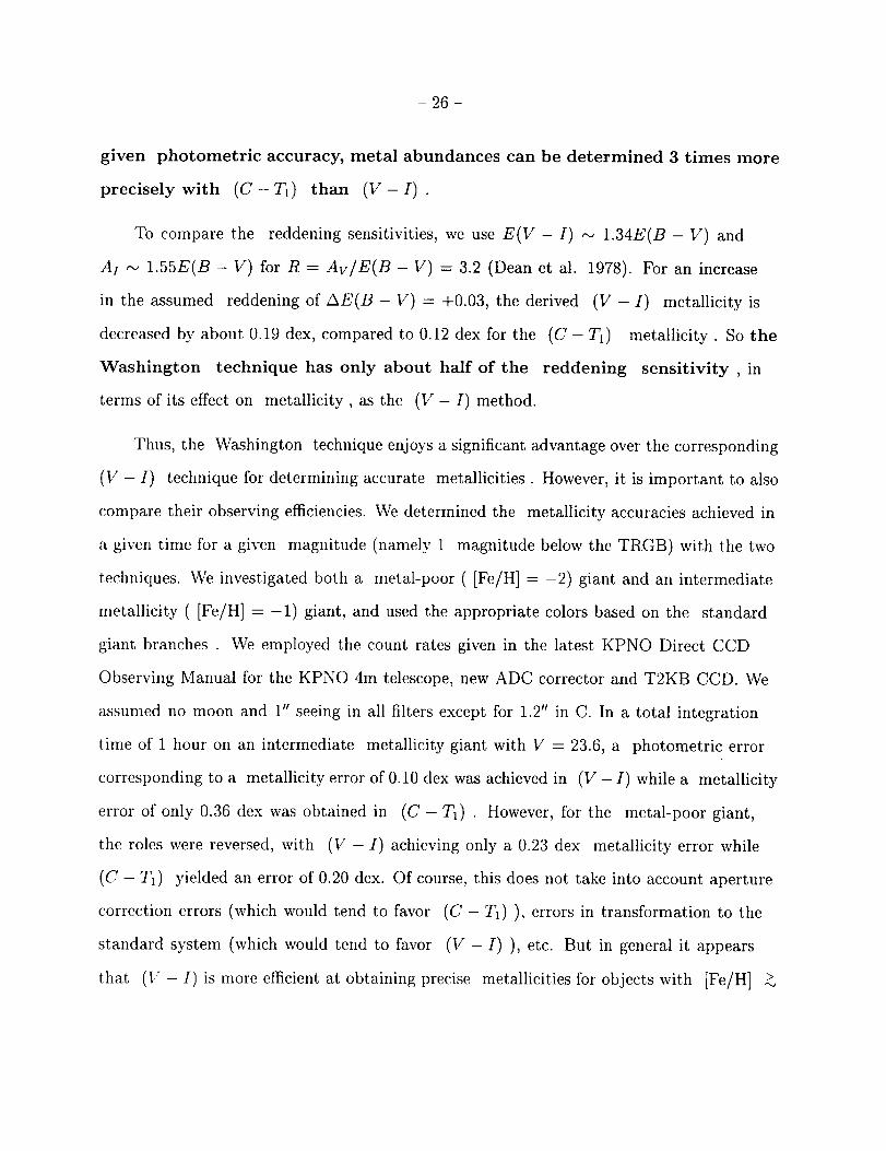
given photometric accuracy, metal abundances can be determined 3 times more

precisely with (C-T1) than (V-I).

To compare the reddening sensitivities, we use E(V - I) ,._ 1.34E(B - V) and

At _ 1.55E(B - V) for R = Av/E(B- V) = 3.2 (Dean et al. 1978). For an increase

in the assumed reddening of AE(B - V) = +0.03, the derived (V - I) metallicity is

decreased by about 0.19 dex, compared to 0.12 dex for the (C - T1) metallicity. So the

Washington technique has only about half of the reddening sensitivity , in

terms of its effect on metallicity, as the (V - I) method.

Thus, the Washington technique enjoys a significant advantage over the corresponding

(V - I) technique for determining accurate metallicities. However, it is important to also

compare their observing efficiencies. We determined the metallicity accuracies achieved in

a given time for a given magnitude (namely 1 magnitude below the TRGB) with the two

techniques. We investigated both a metal-poor ( [Fe/H] = -2) giant and an intermediate

metallicity ( [Fe/H] = -1) giant, and used the appropriate colors based on the standard

giant branches . We employed the count rates given in the latest KPNO Direct CCD

Observing Manual for the KPNO 4m telescope, new ADC corrector and T2KB CCD. We

assumed no moon and 1" seeing in all filters except for 1.2" in C. In a total integration

time of 1 hour on an intermediate metallicity giant with V = 23.6, a photometric error

corresponding to a metallicity error of 0.10 dex was achieved in (V - I) while a metallicity

error of only 0.36 dex was obtained in (C - T1) • However, for the metal-poor giant,

the roles were reversed, with (V - I) achieving only a 0.23 dex metallicity error while

(C - T1) yielded an error of 0.20 dex. Of course, this does not take into account aperture

correction errors (which would tend to favor (C - T1) ), errors in transformation to the

standard system (which would tend to favor (V - I) ), etc. But in general it appears

that (_: - I) is more efficient at obtaining precise metallicities for objects with [Fe/H] >

- 27-

-1.5 while (C - T1) wins for more metal-poor objects. Note that further improvements

in the quantum efficiency of CCDs in the blue-uv will help to improve the C sensitivity ,

but similarly care must be taken to maintain maximum throughput in the optics in this

spectral region.

We note that standard giant branches do exist in If, (B - V) (Sarajedini and Layden

1997). They find that the NGC104 and NGC7078 standard giant branches are separated

by 0.743 magnitudes in (B - V)0 at My = -2, so the corresponding V, (B - V) metallicity

sensitivity is slightly < 2/3 that of the Washington system. A comparison with their

metallicity calibrations used in deriving the equivalent of the SRM method shows that, for

their 6 calibrating clusters , they obtained rms values of from 0.05 to 0.08 dex, roughly

comparable to our values.

4.3. Age Effects

The well known degeneracy between age and metallicity effects for stellar populations

must be addressed. The standard clusters comprising our sample range in age from _ 4

Gyr for NGC2682 to _ 10 - 15 Gyrs for the other clusters (depending on the distance scale

adopted for the GCs and the selected isochrones). The two old open clusters were added to

establish the metal-rich end of the metallicity calibration, with the hope that age effects

would be small. How well was this hope born out? Clearly, given the very old age (_ 10

Gyr) of NGC6791, age effects relative to those for the GCs should be minimal. And indeed

a glance at Figure 6 verifies this. What about the much younger cluster NGC2682? Figure

6 shows that M67 does indeed lie at a slightly bluer color than expected for its metallicity

in all calibrations in which it is involved. However, the effect is small, amounting to only

about 0.1 dex or less. Such an effect could actually be due to our assumed metallicity

being slightly too high. But it is consistent with the younger age causing a bluer RGB and

- 28 -

leading to an underestimate of the metallicity.

Thus, empirically it appears that our metallicity calibrations may be safely applied to

any cluster older than --_ 4 Gyr with only a small effect on the derived metallicity. An

analysis based on Washington isochrones (Lejeune 1997) supports this. These isochrones

include UBVRIJHK as well as CMT1T2 and thus results from different color systems can

be directly compared. An indication of the reliability of these isochrones is given by the

fact that they yield a color difference in (C - T1)0 (at MT1 ---- --2) that is 3.16 times larger

than the corresponding (V- I)0 difference (at MI = -3) between [Fe/H] =-2.2 and

-0.6 (15 Gyr) isochrones, in excellent accord with the results found in the last section for

the differences between the NGC104 and NGC7078 standard giant branches . The 8 and

15 Gyr, [Fe/H] = -1.6 isochrones are separated by 0.093 magnitudes in (C - T1)0 at

M_._ = -2 and by 0.028 magnitudes in (V - I)0 at MI = -3. These color differences

would lead to very similar metallicity "errors" of 0.12 and 0.11 dex, respectively, if gone

unrecognized. Similarly, the differences between 8 and 15 Gyr, [Fe/H] = -0.6 isochrones

are 0.231 and 0.071, leading again to very similar metallicity errors of 0.29 and 0.27 dex,

respectively. As quoted in DCA, the Revised Yale Isochrones (Green et al. 1987) indicate

that a 7 Gyr, [Fe/H] = -1.3 isochrone is 0.05 magnitude bluer in (V - I)0 at MI = -3

than a 15 Gyr isochrone of the same metallicity, leading to a metallicity error of 0.2 alex,

in very good agreement with the trend from the above isochrones. So the age sensitivity

of the \¥ashington standard giant branch technique appears to be very similar to, and

perhaps slightly higher than, that of the (V - I) method for old clusters , and both

systems are more affected by age at higher than lower metallicities.

What about for even younger clusters ? Clearly, by a certain age, the RGB will be

moved sufficiently to the blue relative to an older cluster of the same metallicity that

the effect on the derived metallicity will be significant. The Lejeune isochrones indicate

- 29 -

that the age sensitivity becomes significant for clusters 5 Gyr and younger, especially

for the Washington system. A similar value is obtained from the recent analysis of Bica

et al. (1998) where they compared metallicities derived from the Washington standard

giant branch technique with those available from spectroscopic studies for 5 Galactic

open clusters and 6 LMC clusters whose ages ranged from 1-4 Gyrs (most were _ 2

Gyr). For this sample, a clear trend was found for the Washington standard giant branch

metallicities to underestimate the spectroscopic metallicity by an approximately constant

amount, independent of age. An unweighted mean yielded a difference of 0.41 + 0.21 dex.

Thus, the standard giant branch technique derived here should only be applied to clusters

older than _ 5 Gyr.

We note in passing here that the Lejeune isochrones can also be used to test how

well the Washington system works for deriving ages from main sequence photometry .

VandenBerg et al. (1990) and Sarajedini and Demarque (1990) have shown that the color

difference between the turnoff and the lower subgiant branch is a sensitive and powerful

age indicator. For a [Fe/H] = -0.6 isochrone, this color difference is _0.27 and 0.17

magnitudes in (V - I)0 for a 10 and 20 Gyr population, while in (C - T1)0 the respective

values are 0.71 and 0.47 magnitudes . Thus, the difference in these two values is some

2.5 times larger in (C - 711)0 than (V - I)0, indicating that one could indeed obtain

significantly greater age accuracy using the Washington system for a given photometric

accuracy. These same age isochrones are separated by _0.13 magnitudes in both color

indices for [Fe/H] =-2.2 so for these lower metallicities the age sensitivity is the same.

The Washington system thus holds great potential for deriving accurate ages as well as

metallicities.

- 30 -

4.4. Intracluster Metallicity Dispersion

As developed by DCA, one can use the dispersions in the fit of the standard giant

branches to the data to derive upper limits to the intrinsic metallicity dispersion in each

cluster . In order to investigate this quantity, we have used all cluster stars which fell

between MT, = --1.5 and -2.5, only excluding those stars that fell far away from the RGB.

The standard devation, a(C- T1), about the fitted standard giant branch was calculated

and this value was converted into a metallicity dispersion using our preferred calibration

• The results are displayed in Table 7, where we give the number of stars and the standard

deviations in color and metallicity. Note that the two open clusters did not have sufficient

stars in this part of the RGB to be useful. Also note that this is an upper limit to the

intrinsic metallicity dispersion , as we have not taken photometric errors or contributions

by AGB stars or field stars into account.

The results generally show very small upper limits to the intrinsic metallicity

dispersion of our standard clusters , with a typical limit of _ 0.06 dex. The limit for

NGC5927 is especially large due to the presence of significant field star contamination as

well as differential reddening . Our limits are generally similar to or lower than those

derived for the same clusters by DCA, who found limits of 0.04 dex for NGC104, 0.07 for

NGC1851, 0.06 for NGC6397, 0.05 for NGC6752, and 0.09 for NGC7078. Recall that our

observations were generally centered on these crowded clusters , whereas the DCA data

were generally offset, leading to increased photometric error in the former with respect to

the latter.

Such a procedure can be used to determine the metallicity dispersion in program

objects. In this instance, the measured photometric error can be subtracted in quadrature

from the observed scatter to derive a realistic estimate for any intrinsic dispersion. Indeed,

given a sufficient sample in a system such as a dwarf spheroidal galaxy in which an intrinsic

31-

metallicity dispersion is expected, one could even derive the metallicity distribution of the

giants using this technique , as was done by Geisler and Sarajedini (1996).

5. Simultaneous Reddening and Metallicity Determination

As noted in the Introduction, Sarajedini (1994) devised the simultaneous reddening

and metallicity (SRM) technique to facilitate the determination of these quantities in an

internally consistent manner. The SRM method exploits the fact that the shape and

position of the RGB are dependent on metallicity and reddening. In addition to the

calibration of these quantities using standard RGB sequences, the SRM method also

requires knowledge of the HB magnitude, the color of the RGB at the level of the HB, and

the shape of the RGB.

The first step in establishing the SRM calibration is to estimate the value of 7'I(HB)

for each cluster. This is a rather complicated endeavor because of the diversity of HB types

among the clusters. For the clusters with RR Lyraes, we proceed as follows. Working in

the (T1, C - T1) plane, we fit a cubic polynomial to the HB stars that straddle the RR

Lyrae instability strip. This is done using an iterative 2a rejection algorithm similar to

that utilized for the RGB fits above. Based on the work of Sandage (1990), we have that

the color at the blue edge of the RR Lyrae instability strip is (B - V)0 = 0.18 and the

color of the red edge is (B - V)0 = 0.40. Converting these colors to (C - T1)o with the

transformations of Geisler (1996) gives a mean color of (C - T1)0 = 0.45 for the center

of the instability strip. For those clusters with RR Lyraes, we read off TI(HB) from the

polynomial fits at (C - 7'1)0 = 0.45. The rms of the fit added in quadrature with the

uncertainty in the photometric zeropoint of 0.03 mag is adopted as the error in TI(HB).

In the case of the two clusters with purely blue HB morphologies, NGC6397 and

- 32 -

NGC6752, we use a different approach. First, we fit a polynomial to the blue HB stars

in NGC5272. We then shift the HBs of NGC6397 and NGC6752 in 7'1 until the mean

star-by-star difference with the NGC5272 blue HB fit is minimized. The color shift is set

by the difference in reddening between each cluster and NGC5272. Then, knowing TI(HB)

for NGC5272 from the procedure described above and the shift required to match the

blue HBs, we can infer the values of TI(HB) for NGC6397 and NGC6752. The error is

estimated by adding in quadrature the uncertainty in the TI(HB) value of NGC5272 and

the uncertainty in the shift.

There are 4 clusters with purely red HBs in our sample. We are omitting NGC2682

from the SRM calibration because its RGB is too sparsely populated. In the case of these

clusters, we construct 711 mag histogram distributions of the HB stars. Fitting a gaussian

curve in the region of the peak in these histograms yields the value of TI(HB), while the

error in TI(HB) is given by the dispersion in the fitted gaussian divided by the square

root of the number of points used in the curve fit. The resulting error ends up being

quite small (typically < 0.01 mag) because of the large number of points on the red HB.

The only significant error in the TI(HB) of the red HB clusters is that associated with

the photometric zeropoint, which we estimate to be _0.03 mag. We note in passing that

fitting the Gaussian in the region of the histogram peak minimizes the uncertainties in the

value of TI(HB) introduced by the evolution of stars away (brightward) from the Zero Age

Horizontal Branch.

Once we have settled on values of TI(HB) for each cluster, then we utilize the

polynomial RGB fits to read off the (C - T1)g value, which is converted to (C - T1)0,9 by

applying our adopted reddenings. We can also construct the magnitude difference between

the HB and RGB at (C - T1)0 = 2.4 (i.e. AT2.4). Both of these quantities, (C - T1)g and

AT2.4 vary with metal abundance, and are listed in Table 8 along with the other measured

- 33 -

parameters. Performing a weightedleast squaresfit givesus the two relations that are

central to the SRM method,

[Fe/H] = a, + bl x (C - T1)0,9 + ca x (C - T1)_,g + dl x (C - T_)_,g (3)

[FelH] = a=+ t,2× /',T2.4+ × + × (4)

Table 9 gives the values of these coefficients for the various metallicity scales considered

herein, while Fig. 7 illustrates the relations. The metallicity errors are taken from Zinn &

West (1984) for the Z85 abundances and Rutledge et al. (1997) for the CG97 and HDS

abundances.

The reader is referred to the work of Sarajedini (1994) for a detailed description of how

to apply the SRM method. In summary, one needs a polynomial or fiducial representation

of the cluster RGB sequence as well as estimates for the observed values of TI(HB) and

(C- T1)g. Then, an iterative procedure can be set up that utilizes these observed properties

in conjunction with the two equations above to provide estimates of the cluster reddening

and metallicity. In addition, Monte Carlo simulations are used to determine the uncertainty

in these quantities. Given a well-determined RGB sequence with errors of 0.03 mag in

TI(HB) and 0.03 mag in (C - T_)9, we expect metallicity errors of 0.15 dex in [fe/H]

and reddening errors of 0.05 mag in E(C - T1) (0.025 mag in E(B-V)). As for the effects

of cluster age, Sarajedini & Layden (1997) and Mighell et al. (1998) have shown that the

SRM method is insensitive to age for clusters _4 Gyr and older.

- 34 -

6. Additional Metallicity, Reddening and Distance Determination Techniques

6.1. Metallicity Determination from the Slope of the Red Giant Branch

Tile work of Hartwick (1968) illustrated the suitability of the RGB slope as a metallicity

indicator. In the present work, we define the RGB slope (S-2) as

-2.0

8-2 = [(C- T1)g - (C- T1)-2]' (5)

where (C - T1)-2 is the color of the RGB at 2 magnitudes above the HB. This quantity is

well correlated with metal abundance; as such, we can construct the following relation -

[Fe/H] = a + b × S-2 + c z $2_ (o)

for the three metallicity scales. Table 10 lists the values of these coefficients while Fig. 8

illustrates the relations. The RGB slope method of metallicity determination is especially

useful since it does not require knowledge of the reddening or the distance. Furthermore,

Mighell et al. (1998) have shown that, in the B - V passbands, it is insensitive to age for

clusters older than _4 Gyr. If the values of (C - T1)g and (C - T1)-2 can be determined

with an error of +0.03 mag, then the resultant error in [Fe/H] is approximately 0.08 dex.

6.2. Metallicity Determination from the Magnitude of the Red Giant Branch

Bump

As a star evolves up the first ascent RGB, it reaches a point where its evolution pauses

or reverses course for a short time, after which it resumes its brightward movement in the

H-R Diagram (Thomas 1967; Iben 1968). This phenomenon leads to a clumping of stars

along the RGB. When a luminosity function (LF) is constructed, this clump manifests itself

as a bump in the LF, hence the name 'RGB bump.'

- 35 -

From theoretical considerations,the luminosity of the RGB bump is dependenton age

and abundance(Iben 1968,Fusi Pecciet al. 1990). However,sincethe absolutezeropoint

of the theoretical RGB bump luminosity is uncertain, it is moreusefulto measurethe RGB

bump magnitude relative to that of the HB (i.e. ATl(Bump - HB)). In these terms, as a

cluster's age and/or metallicity increases, ATl(Bump - HB) also increases. For clusters

that are older than ,-_10 Gyr, the effect of age on the absolute magnitude is negligible (A1ves

& Sarajedini 1998); as a result, we can utilize the magnitude difference between the RGB

bump and the HB as a metallicity indicator as proposed by Fusi Pecci et al. (1990) and

parameterized by Sarajedini & Forrester (1995).

To isolate the location of the RGB bump, we proceed in the same manner as Sarajedini

K: Norris (1994). First, we construct a cumulative LF of the RGB stars. As illustrated in

their Fig. 15, the RGB bump clearly stands out in such LFs. After fitting a 'continuum'

to the LF around the region of the bump, we subtract this off resulting in a flattened RGB

LF. The maximum point in this flattened LF represents the faintest extent of the RGB

bump, while the zero crossing immediately brightward represents the onset of the bump as

one proceeds fainter from the RGB tip. We therefore adopt the magnitude midway between

these two points as the value of Tl(Bump), which is then coupled with Tl(HB) to produce

AT1 (Bump - HB). The error in 7'1(Bump) is half the distance between the maximum and

the zero-crossing multiplied by 0.68 to simulate a 1-_ uncertainty.

As in the case of the RGB slope, we parameterize tile variation of the RGB bump with

metallicity using the following relations.

[Fe/Hl = a + b x ATI + C × AT 2, (7)

where AT1 is the difference in magnitude between the bump and the HB; the fitted

coefficients are listed in Table 11. Figure 9 shows the fitted points and tile resulting

relations. If tile value of AT1 can be measured to +0.1 magnitude , then the metallicity

determined from the RGB Bump will have an uncertainty of ,_0.1 dex.

Our CMDs are sufficiently populous that, at least in several instances, we see evidence

of a similar LF enhancement on the AGB _ 1 magnitude above the HB. The best cases

are NGC104, NGC5272 and NGC7078. We believe that this feature is the AGB bump,

due to a phenomenon similar to that which produces the RGB bump. Such a feature has

recently been identified in populous LMC field star CMDs (Gallart 1998) and may well be

responsible for the 'VRC' suggested by Zaritsky & Lin (1997) as being due to a possible

foreground galaxy.

6.3. Reddening Determination from the Red Edge of the Blue Horizontal

Branch

The temperature limits of the RR Lyrae instability strip are well-defined, both

theoretically and observationally (see Sandage 1990). Previous studies have exploited

this fact to derive the reddening of a cluster , given a large sample of RR Lyraes and

giants along the BHB: the observed color limit between the variables and non-variables is

compared to the intrinsic color limit, directly yielding the reddening. We have undertaken

a similar analysis, using the six standard clusters (NGC1851, NGC4590, NGC5272,

NGC6362, NGC6752 and NGC7078) which have both RR Lyraes and BHB stars. NGC6752

in fact does not have RR Lyraes but does appear to have BHB stars that lie very near the

edge of the instability strip. On the other hand, the reddest BHB stars in NGC6397 fall

substantially blueward of the instability strip.

It is clear from Figure 2 that the BHB stars in these clusters generally lie in a fairly

tight sequence, that the RR Lyraes fall in a more scattered distribution from fainter, redder

colors to brighter, bluer colors, and that the color limit between these two types of stars is

- 37-

reasonablywell defined.We derivedthis limit in (C - T1) and converted it to (C - T1)0

using the cluster reddenings . The six clusters have < (C - 7'1)o >= 0.17, with a _ of

only 0.03. Sandage (1990) gives this limit as (B - V)0 = 0.18 which is (U - T_)0 =0.22

using the conversion of Geisler (1996). Giving some weight to this determination, we adopt

(C - T_)0 = 0.18 + 0.04 for the intrinsic color of the red edge of the BHB. We can then use

this value to derive the reddening to a program object which has a sufficient number of

BHB and RR Lyrae stars, with an estimated error of c,(E(B - V)) = 0.025. This technique

can be used to supplement the reddening derived from the SRM method described above.

6.4. Distance Determination from the T1 Magnitude of the Tip of the Red

Giant Branch

The I magnitude of the TRGB has become an increasingly popular standard candle in

recent years. The work of Lee et al. (1993) and others has shown that this is indeed a very

useful distance indicator. We have investigated the analogous use of the T1 magnitude of

the TRGB as a distance indicator.

A glance at Figure 4 suggests that MTlrRc.u has at most a very small dependence on

metallicity for metal-poor clusters ( [Fe/H] _< -1.15). We have determined this value

for the 6 standard clusters falling in this regime. A mean MTlrRc.u = --3.22 + 0.11(a) is

obtained. The small rms indicates that this should indeed be a useful distance indicator

for such objects. Clearly, though, at higher metallicities MTIrRc.B increases rapidly with

increasing metallicity and is not useful. Indeed, such behavior is also seen for MITRc.B for

[Fe/H] _-0.75.

We can use the Bertelli et al. (1994) isochrones to investigate theoretical predictions

concerning how MT_rRa B depends on age and metallicity . Geisler (1996) has shown that

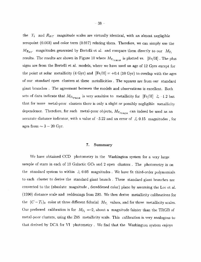
- 38 -

the T1 and RKC magnitude scales are virtually identical, with an almost negligible

zeropoint (0.003) and color term (0.017) relating them. Therefore, we can simply use the

MR_,c magnitudes generated by Bertelli et al. and compare them directly to our MT1

results. The results are shown in Figure 10 where MT1TRaB is plotted vs. [Fe/H] . The plus

signs are from the Bertelli et al. models, where we have used an age of 12 Gyrs except for

the point at solar metallicity (4 Gyr) and [Fe/H] = +0.4 (10 Gyr) to overlap with the ages

of our standard open clusters at these metallicities. The squares are from our standard

giant branches . The agreement between the models and observations is excellent. Both

sets of data indicate that MT1TRGB is very sensitive to metallicity for [Fe/H] > -1.2 but

that for more metal-poor clusters there is only a slight or possibly negligible metallicity

dependence. Therefore, for such metal-poor objects, MTITRGB can indeed be used as an

accurate distance indicator, with a value of-3.22 and an error of < 0.15 magnitudes , for

ages from _ 3 - 20 Gyr.

7. Summary

We have obtained CCD photometry in the Washington system for a very large

sample of stars in each of 10 Galactic GCs and 2 open clusters . The photometry is on

the standard system to within < 0.03 magnitudes. We have fit third-order polynomials

to each cluster to derive the standard giant branch . These standard giant branches are

converted to the (absolute magnitude , dereddened color) plane by assuming the Lee et al.

(1990) distance scale and reddenings from Z85. We then derive metallicity calibrations for

the (C - T1)0 color at three different fiducial MTI values, and for three metallicity scales.

Our preferred calibration is for MT_ -----2, about a magnitude fainter than the TRGB of

metal-poor clusters, using the Z85 metallicity scale. This calibration is very analogous to

that derived by DCA for VI photometry . We find that the Washington system enjoys

39-

three times the metallicity sensitivity of the VI technique . It is also lesssensitiveto

reddening. The Washington standardgiant branch metallicity techniqueis also superior

to the Washington two-colordiagram techniquein virtually all respects.The standard

giant branch techniqueis immuneto ageeffectsfor objects older than _ 5 Gyr. We derive

upper limits of typically 0.06dex for any intrinsic metallicity dispersion in the standard

clusters.

We also use the standard giant branchesto derive a method analogousto that of

Sarajedini (1994)for determining both the metallicity and reddeningsimultaneously.The

magnitude differencebetweenthe HB and the RGB bump, and the slopeof the RGB, are

alsofound to besensitive metallicity indicators. In addition, reddeningcan bedetermined

from the color of the red edgeof the blue HB. Finally, the T1 magnitude of the TRGB is

an accurate distance indicator for objects more metal-poor than [Fe/H] _ -1.2 and older

than 3 Gyr. An analysis of available isochrones indicates that the Washington system also

holds great potential for deriving accurate ages as well as metallicities.

Gary Da Costa and Taft Armandroff provided much of the inspiration for this work

from their original study in the V,I system (DCA). We thank Hugh Harris for a critical

reading of a preliminary version of this manuscript. The authors would like to thank

Juan Clari/t and Cristina Torres for providing important photoelectric data in advance of

publication. Juan Clari_ and AndrOs E. Piatti also very kindly obtained one of the CCD

fields for us. Pat Durrell allowed us to obtain another field during telescope time set aside

for his thesis. Peter Stetson, as always, has been very generous in allowing the use of his

own very useful programs. Jim Roberts and Eva Grebel are acknowledged for their initial

work on another project which helped to launch the present one. The cluster photometry

can be obtained from the first author upon request. This research is supported in part by

NASA through grant No. GO-07265.01-96A (to DG) and HF-01077.01-94A (to AS) from

- 40 -

the SpaceTelescopeScienceInstitute, which is operatedby the Associationof Universities

for Researchin Astronomy, Inc., under NASA contract NAS5-26555.This researchis

supported in full by E. Geislerthrough herconstant loveand encouragement.

-41 -

REFERENCES

Ajhar, E.A., Grillmair, C.J., Lauer, T.R., Baum, W.A., Faber, S.M., Holtzman, J.A.,

Lynds, C.R., & O'Neil, E.J. 1996, AJ, 111, 1110

Alves, D., & Sarajedini, A. 1998, in preparation

Armandroff, T.E. 1989, A J, 97, 375

Armandroff, T.E., & Da Costa, G.S. 1991, A J, 101, 1329

Armandroff, T.E., Da Costa, G.S., Caldwell, N., & Seitzer, P. 1993, A J, 106, 986

Armandroff, T.E., & Zinn, R. 1988, A J, 96, 92

Bertelli, G., Bressan, A., Chiosi, C., Fagotto, F., & Nasi, E. 1994, A&:AS, 106, 275

Bica, E., Geisler, D., Dottori, H., Clari£, J.J., Piatti, A.E. & Santos, J.F.C. Jr. 1998, A J,

in press

Brown, J.A., Wallerstein, G., & Zucker, D. 1997, AJ, 114, 180

Canterna, R. 1976a, A J, 81,228

Canterna, R. 1976b, PhD. thesis, University of Washington

Canterna, R., Geisler, D., Harris, H.C., Olszewski, E., & Schommer, R. 1986, A J, 92, 79

Carney, B.W., Storm, J., & Jones, R.V. 1992, ApJ, 386, 663

Carretta, E., & Gratton, R.G. 1997, A&AS, 121, 95 (CG97)

Chaboyer, B. , Demarque, P., Kernan, P. J., & Krauss, L. M. 1998, ApJ, 494, 96

Clari_, J.J., & Torres, M.C. 1998, in preparation

Da Costa, G.S., & Armandroff, T.E. 1990, A J, 100, 162 (DCA)

Dean, J.F., Warren, P.R., & Cousins, A.W.J. 1978, MNRAS, 183, 569

Dinescu, D.I., Demarque, P., Guenther, D.B., & Pinsonneault, M.H. 1995, A J, 109, 2090

- 42 -

Friel, E.D., & Geisler,D. 1991,AJ, 101,1338

Frogel,J.A., Cohen,J.G., & Persson,S.E. 1983,ApJ, 275,773

Fusi Pecci,F., Buonanno, R., Cacciari, C., Corsi, C.E., Djorgovski, S.G., Federici, L.,

Ferraro, F.R., Parmeggiani, G., & Rich, R.M. 1996, A J, 112, 1461

Fusi Pecci, F., Ferraro, F.R., Crocker, D.A., Rood, R.T., & Buonanno, R. 1990, A&A, 238,

95

Gallart, C. 1998, ApJ, 495, 43

Geisler, D. 1986a, PASP, 98, 762

Geisler, D. 1986b, PASP, 98, 847

Geisler, D. 1990, PASP, 102, 344

Geisler, D. 1994, in The Local Group: Comparative and Global Propeties, ESO Conf. Proc.

No. 51, ed. A. Layden, R.C. Smith & J. Storm (Garching:ESO), 141

Geisler, D. 1996, A J, 111,480

Geisler, D., Clarid, J.J., & Minniti, D. 1991, A J, 102, 1836 (GCM)

Geisler, D., Clari£, J.J., & Minniti, D. 1997, A J, 109, 799

Geisler, D., Lee, M.G., & Kim, E. 1996, A J, 111, 1529

Geisler, D., Minniti, D., & Clari_, J.J. 1992, A J, 104, 627

Geisler, D., Piatti, A.E., Clari_, J.J., & Minniti, D. 1995, A J, 109, 605

Geisler, D. & Sarajedini, A. 1996, in Formation of the Galactic Halo...Inside and Out, ASP

Conf. Set., no.92, ed. H. Morrison & A. Sarajedini (San Francisco:ASP), 524

Green, E.M., Demarque, P., & King, C.R. 1987, The Revised Yale Isochrones and

Luminosity Functions (Yale University Observatory, New Haven)

Harris, H.C., & Canterna, R. 1977, A J, 82, 798

- 43 -

Hartwick, F.D.A. 1968,ApJ, 154,475

Iben I. Jr. 1968,Nature, 220,143

Lee.,M.G., Freedman,W.L., & Madore, B.F. 1993, ApJ, 417, 553

Lee, Y.-W., Demarque, P., & Zinn, R. 1990, ApJ, 350, 155

Lejeune, T. 1997, Ph.D. thesis, Universite Louis Pasteur, Strasbourg

McWilliam, A., Geisler, D., & Rich, R.M. 1992, PASP, 104, 1193

Mighell, K. J., Sarajedini, A., & French, R. S. 1998, in preparation

Minniti, D., & Clari_, J.J. 1989, ApJ, 341,186

Minniti, D., Geisler, D., Peterson, R.C., & Clari£, J.J. 1993, ApJ, 413, 548

Pont, F., Mayor, M., Turon, C., & VandenBerg, D. 1998, A&Ap, 329, 87

Reid, I.N. 1997, A J, 114, 161

Rood, R.T. 1978, in Globular Clusters, NATO Advanced Study Institute

Rutledge, G.A., Hesser, J.E., & Stetson, P.B. 1997, PASP, 109, 907.

Sandage, A.R. 1990, ApJ, 350, 603

Sandage, A.R., & Smith, L.L. 1966, ApJ, 144, 886

Sarajedini, A. 1994, A J, 107, 618

Sarajedini, A., & Demarque, P. 1990, ApJ, 365, 219

Sarajedini, A., & Forrester, W. L. 1995, AJ, 109, 1112

Sarajedini, A., & Layden, A. C. 1997, AJ, 113, 264

Sarajedini, A., & Norris, J.E. 1994, ApJS, 93, 161

Searle, L., & Zinn, R. 1978, ApJ, 225, 357

Sneden, C., Kraft, R.P., Prosser, C.F., &Langer, G.E. 1991, A J, 102, 2001

- 44 -

Sneden,C., Kraft, R.P., Shetrone,M.D., Smith, G.H., Langer,G.E., & Prosser,C.F. 1997,

AJ, 114,1964

Stetson,P.B. 1987,PASP,99, 191

Thomas, H.-C. 1967,Z. Ap, 67,420

Trefzger,C.F. 1981,in AstrophysicalParametersfor Globular Clusters, IAU Coll. No. 68,

ed. A.G.D. Philip and D.S. Hayes(Davis,Schenectady),33

Tripicco, M.J., Bell, R.A., Dorman, B., & Hufnagel,B. 1995,AJ, 109,1697

Twarog, B.A., Ashman, K.M., & Anthony-Twarog, B.J. 1997,AJ, 114,2556

VandenBerg,D.A., Bolte, M., & Stetson,P.B. 1990,AJ, 100,445

Wallerstein, G., & Helfer, H.L. 1966,AJ, 71,350

Zaritsky, D., & Lin, D.N.C. 1997,AJ, 114,2545

Zinn, R. 1985,ApJ, 293,424 (Z85)

This manuscript waspreparedwith the AAS LA_X macros v4.0.

- 45 -

Figure Captions

Fig. 1.-- a. The differencebetweenthe (C-T1) valuederivedfrom CCD and photoelectric

photometry, asa function of the photoelectricvalue,for giants in NGC6397in common, b.

As for a). except for the T1 magnitude .

- 46 -

Fig. 2.-- T1 vs. (C-T1) color-magnitude diagram for the standard clusters, a. NGC104

b. NGC1851 c. NGC2682 NB - in this diagram, CCD observations are denoted by squares

and photoelectric data by crosses, d. NGC4590 e. NGC5272 f. NGC5927 g. NGC6352 h.

NGC6362 i. NGC6397 j. NGC6752 k. NGC6791 1. NGC7078

Fig. 3.-- T_ vs. (C- T1) CMD for the standard clusters showing the standard

giant branches . Filled squares are observations used in the fit, open squares are unused

or rejected stars. Large crosses indicate photoelectric observations. The solid curve is the

standard giant branch fit. a. NGC104 b. NGC1851 c. NGC2682 d. NGC4590 e. NGC5272

f. NGC5927 g. NGC6352 h. NGC6362 i. NGC6397 j. NGC6752 k. NGC6791 1. NGC7078

Fig. 4.-- The Washington standard giant branches in the ( MT, , (C-Zl)o) plane. At _IT1

= 1.5, the standard giant branches are (from left to right): NGC7078, NGC4590, NGC6397,

NGC5272, NGC6752, NGC1851, NGC6362, NGC104, NGC5927, NGC6352, NGC2682 and

NGC6791_

Fig. 5.-- A comparison of the same VI and Washington standard giant branches. The VI

data are taken from DCA and plot MI vs. (V - I)0. The Washington data plots MT1 vs.

(C- T1)0 • The clusters are (from left to right): NGC7078, NGC6397, NGC6752, NGC1851

and NGC104. The Washington standard giant branches are much more widely separated

than the VI RGBs.

Fig. 6.-- Metallicity calibrations for various combinations of fiducial magnitude and

metallicity scale, a. ( MTI =-2.5,Z85) b. (-2.5,CG97) c. (-2.5,HDS) d. (-2,Z85). This

is our preferred calibration. The discarded point (NGC5927) is shown in parantheses. The

plus signs show the DCA standard giant branches, using Me =-3 and adding 1 to (V-I)0

. e. (-2,CG97)f. (2,HDS) g. (-1.5,Z85)h. (-1.5,CG97)i. (-1.5,HDS)

- 47 -

Fig. 7.-- Calibration of the SRM method for deriving reddening and metallicity

simultaneously. [Fe/H] (for three different metallicity scales)is shown as a function of

the CMD parameters(C - T1)o,9 and ATz4 for the standard clusters .

Fig. 8.-- Calibration of the RGB slope for deriving metallicity. [Fe/H] (for three different

metallicity scales) is shown as a function of the RGB slope.

Fig. 9. Calibration of the RGB bmnp for deriving metallicity. [Fe/H] (for three different

metallicity scales) is shown as a function of AT1 (Bump-HB).

Fig. 10.-- ]_J!T 1 at the RGB tip as a function of metallicity. The squares are the standard

giant branches ; the plus signs are from the model isochrones of Bertelli et al. (1994). For

metallicities < -1.2, MTIrRa, is nearly constant and can be used as a distance indicator.

.3

.2

-.I

I I I I I

(C-TI) CCD vs. PEI I I l I I I

o

o Or_

o o 0

o o °o K3

I ! I I I ' ' ' ' I

2 3

(C-TI)(PE)

I I

NGC6397

I I I I

4

.3

.2

-.19

T1 CCD vs. PE

' ' ' ' I ' ' ' ' I _ ' ' ' I ' ' ! I

NGC6397

i l I , I i I , , I , , I , I , , , ,

10 11 12 13

TI(PE)

.... I .... I .... I " .' ' ' I ....

• ). N¢Ci 04 ::_:.

.._..¢

• _,_:

:i"2. '_ , , i .... i ....

1 3 4

(c-it)

-1

.... i .... I .... I .... i ' .' • •

c). NCCZdOZ

..-..

..-2_-"- _:-...-

"" "_-.2:..'.

--.. ,-_.. "'._

.'" "'." i ; _::;-."_'_.-• :.. ..

i i • . l .... I , • . I .... I ....

o i z 3

(C-tL)

2O

-1

.... I .... i .... I .... i ....

b)• NGC| 85L

,.. ",

• ._: . -: .., .-L. .. -. -

,_'_.. _,:J -.." . ,..

• ... ;.,._ :-;.. ., .

• :"._;_ ...."_.:-.-.• • . ..• .-._: ,.-..':.-...

, , , i I , i i , I .... I .... I ....

o 1 2 3

(c-it)

.... i .... I .... I .... I ....

d). NGC4590lZ.

• . . .-.!_.'."

.. t_ _ •

._e,;, _" ':'t-_" .._ .: . . . ."

- ..-. :... • ..,,,... - . • .

.. ':..': , 2_: " ' _ ".." . • . • "_

x'_. . , ........ ...._.;, .. -- . -. • --,• ..,._,. _,.. . .' • . -,

....-_ ,:- ._.-... ,. .... _ , _.

_:".-( ._:;_• ..

• -:

-i o t z 3

(C-TI)

la

t). NGC6Z';,j

.', . '_i.L_, :{' • .

• i i | , , . i I , , . i I , , , , I . i ,

o 1 z 3

¢c-rt)

t{ .... i .... _ .... i .... i • • • ,i). NgCS3b2

. . .. .

:IL ; *

.-:. -¢-...._.,.-...

' • • l l , • l , I , . l l I , . i l I , , l iI I 3 4

.... I .... i .... i .... i • , • ,

._. .."

: " .Z' .-';' ":

..... ":,'_, ._..:_:.:.:• . •..:-:..-.," "'.;_: _ .' . .'.,... :_,_. _ . /, .

i .zo I • i I , . i , I , I• , , • i , . I i i , .

o I _ 3

(C-tt)

17,-"

-1

.... t .... I .... I .... I ....

|). N6C6397

• "#.

4 m B-

...," ,,.-',_t__'_.:..': •... _r_.._ , ' . ,_.

:.:_ '_ ';:,': ...

.... I , , , i | i i • , I .... I ....

0 l z 3

(C-TL)

2O

-I

.... I .... I .... I "-' ' ' I ....

k). IqGCi5791 I •

: " -" • . ." . :-,_,...t'"

, ....:_,:.:- .':.. -._,.m • . _.,, _-_.':,-...:..--.:.i,_,_.

• .-_,.:_.;..:._,."-_.:_._: ,.; . .;• .o .c -.,: • .. :: - -. • .

? ."..',:...'". , . .'."

.... I , , * , | , • • , I .... I ....

0 I 2 3

(C-?L)

15

l"t.I

-1

j). NGC$752

.... I I , , , I , , • • i .... i ....

o t Z 3

(c-t'[)

20

-I

.... I .... I .... I .... I .... |

1.:.:_,_

.... I "

0 Z 3

¢-TL )

.... I .... I .... I .... I ....

a). NGC104

.. °

X_.'_ :'_ "

2 Z._ 3 3.5

(¢-Tt)

' I .... I .... ! .... ! .... I • • •

b), NGCISS] . ..

. " - . •

-."° °X

1.5 Z 3.5 3 3.5

(C-TL)

12

13

15

10

• " I .... I .... I .... I .... I •

c). NGC368Z

a

• I,,,:1.,,,I .... I.,.ll ,

].5 _ 2.5 3 3.5

(c-rt)

• _:,[ _cc_s_o' " ' ' .... ' .... ' ..... °

• _ >'0' "_<

• "X o ° • °

:,;_.

..._- -. .

. ": . <.- . . •

! • ...*. . . . .

.5 1 1.5 2 Z.5

(c-t't)

_.. .... I .... I .... I • ' ' " I ....12

• " .,r

• i;._o'" .'o • "

14 " °" ; "" •o o_

. _.. _,_ .. . •

..." • .--_ .-s :: -._- _ :

_, • oo w o " °

16

1 [,_ 2 2.s 3

(C-T1)

t4

' " I .... l .... l .... I .... I '

|). NGC4352

• X • .X

X X°

° °r s° "

""_ " "_ "_'" " " " ".... i .• "1".+,,,._=',--J . " , . i .

2 2,5 3 3.5 4

(¢-_t)

._ " .° °

172,5 3 3+5 • 4.5

(c-Tx)

' • I .... I .... I .... I .... I • '

h). P+cca3+nz

xoX ° •

. o°,p o

," ,to °_ . o_

&.._)."

t °o_._* ° °o ° ° ° .H

; t.; l.. . .:,,+__....,... :, :-...,.1.5 2 2.5 3 3+5

(C-TI)

' ,.')'_o,,-_'/,"• . , .... , • . ,,_._ ..../." X .- X ;

1.$ _ 2.6 3 3._

(c-lrl)

.... i • , ' I .... ; .... i ....k). NGCeTo1 "

12

13

1¢ , ,[.s 2 z._ 3 3.5

(c-rx)

.... i .... I .... I .... i .... ! '

[.s | 2.5 3 3.5

(C-Tt)

' • ' ' ' I .... I .... I .... I ....

1). NCCTO'/e11

• . _,< " "°

• ." • _,_-..

. " x

14 . "

. - -.

0

tS[-- " . . . {. ""

l_'"-':"":'": . .'! -.. • . - .?t .16

.. " . ,,e .[ .... , ._L e', , .,'." . , , . .'-, . . ,

(¢-I"a)

A

-4

-2

Standard Giant Branches in the Washington System

' ' I ' _ ' ' I ' '

2 3

(C-T1)o

I

-4

-2

Comparing CTI and VI SGBs

I ' ' ' ' I ' ' ' ' I ' ' ' '

V-I

, / / 11 C-T1i/ / / //

/1 IIIi II x/"_"

iI /I /I ii I

/ / / .,

t//1/J / I/ 11/

l/lit�l/i/ /11

iiiiii i I i/

/11/I / I/

i I i I iI i I

,_/',//

,4",,;"/,,,;; // / / /

'"'"SJ//1 2 3 4

Dereddened Color

4,

i

3._

3

2.1

4 ,

v

' " I I I ' '

).

J,.I I,,,.I.*

-2 -L 0

[P_/K](ZS6)

' I I I

b).

fI I i a * • I . *

-2 -! 0

[re/e](ccsT)

4 .• I I

] _ i I i

-2 -L

(re/el(aDs)

o

C_

¢=

v

...?...-

¢= 2

• ! I I ° •

d).

2

l,: ' • I .... I , . , _ | i i

-I -I 0

[ _'e/I] (z66)

4 , , I

i).

! I " '

,,I,, I Ii,

-Z -I 0

[re/ul(cGoT)

a::: 2

' I I I • r

I).

I--1

-S --I 0

[ F_/H)(HDS)

.-_ 3

v

1 J

' I I

-z -I o

[r_/e](zee)

' ' I I I ' '

5).

D _

* (_ i i * s ] * * * * " '

-z -1 o

[ re/el (coo'r)

I I I

d).

r_ (c_)

-2 -I o

[_e/n](uos)

0

mo -1

-2

0

m¢_ -1

-2

0

mo -1

-2

(C - T1)o,g AT2. 4

0

-2

0

-2

0

-2

Z85

CG97

- _ HDS -

2 3 4

RGB Slope

0

0

0

, , , I , , I , I r , t , I- CG97

I I t t

, , I , , , j I , , , t I , , , ,

-0.5 0.0 0.5

ATI(Bum p - HB)

'/

E---

-3

-2

-1

I

D

EZ3D

I-2

I I

Iz3

I I

EZ3

I I I I I-1

[r_/H]

-4-

D -t-

I I I

(_

D-t-

E3

TABLE 1

PARAMETERS FOR THE STANDARD CLUSTERS

NGC E(B-V) (m - M)v [Fe/Hlz85 [Fe/H]cG97 [Fe/H]HDS

104 (47 Tuc) 0.04 13.51 -0.71 -0.78 -0.761851 0.02 15.45 -1.15 -1.03

2682 (M67) 0.05 9.70 -0.05 -0.05 -0.05

4590 (M68) 0.03 15.14 -2.09 -2.00 -2.03

5272 (M3) 0.01 15.11 -1.665927 0.45 16.08 -0.30 -0.64 -0.1

6352 0.24 14.57 -0.51 -0.70 -0.58

6362 0,11 14.70 - 1.08 -0.99 - 1.00

6397 0.18 12.40 -1.91 -1.76 -1.90

6752 0.04 13.19 -1.54 -1.24 -1.51

6791 0.13 13.60 +0.25 +0.25 +0.25

7078 (M15) 0.10 15.41 -2.15 -2.02 -2.24

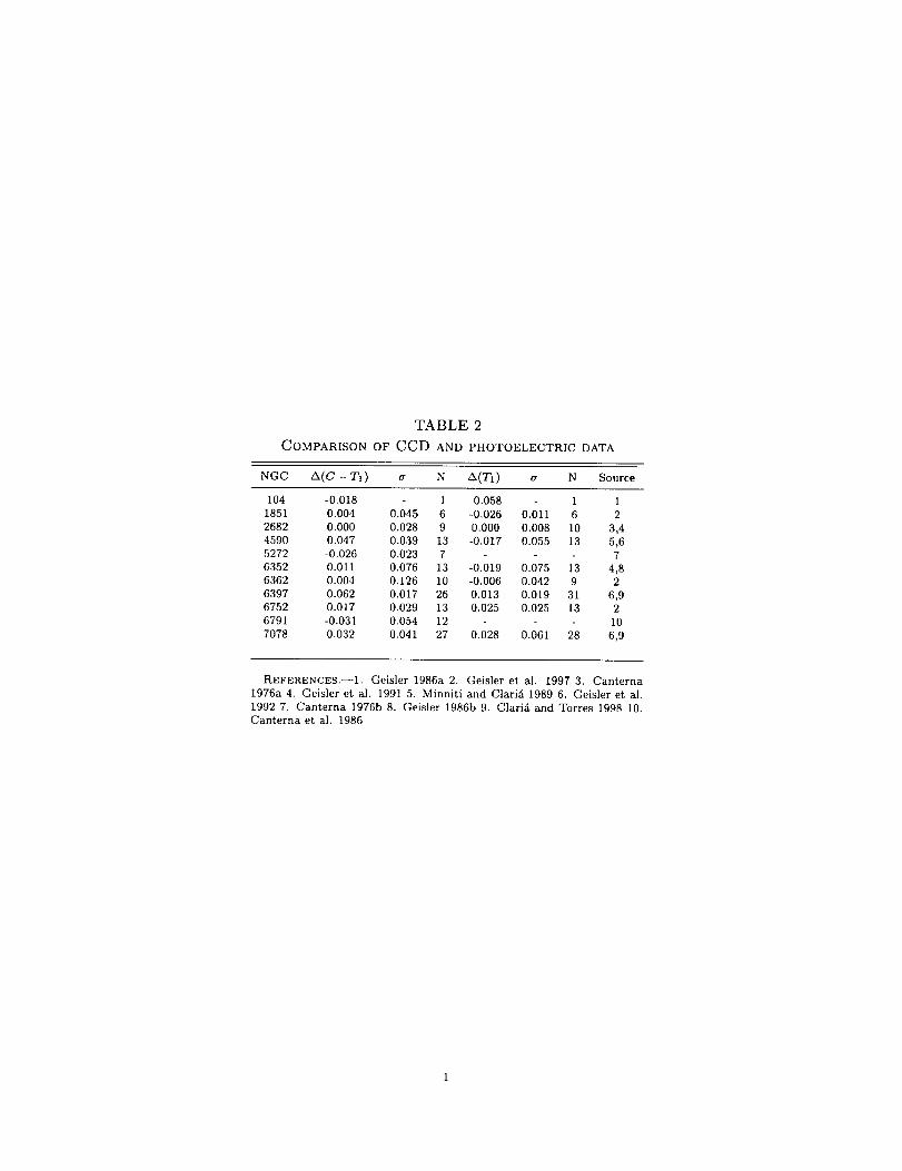
TABLE 2

COMPARISON OF CCD AND PHOTOELECTRIC DATA

NGC A(C -- 7'1) cr N A(T1) a N Source

104 -0.018 1 -0.058 1 1

1851 0.004 0.045 6 -0.026 0.011 6 2

2682 0.000 0.028 9 0.000 0.008 10 3,4

4590 0.047 0.039 13 -0.017 0.055 13 5,65272 -0.026 0.023 7 7

6352 0.011 0.076 13 -0.019 0.075 13 4,86362 0.004 0.126 10 -0.006 0.042 9 2

6397 0.062 0.017 26 0.013 0.019 31 6,96752 0.017 0.029 13 0.025 0.025 13 2

6791 -0.031 0.054 12 10

7078 0.032 0.041 27 0.028 0.061 28 6,9

REFERENCES.--1. Geisler 1986a 2. Geisler et al. 1997 3. Canterna

1976a 4. Geisler et al. 1991 5. Mianiti and Clari_ 1989 6. Geisler et al.

1992 7. Canterna 1976b 8. Geisler 1986b 9. Clari_ and Torres 1998 10.Canterna et al. 1986

TABLE 3POLYNOMIALCOEFFICIENTS

NGC T1 Offset a b c d

104 12.5

1851 15

2682 10

4590 15

5272 15

5927 15

6352 15

6362 156397 12.5

6752 12.5

6791 14

7078 15

2.408 -0.470 0.0992 -0.0107

1.808 -0.284 0.0812 -0.0233

2.350 -0.361 0.0483 0.0028

1.353 -0.172 0.0315 -0.0137

1.489 -0.205 0.0437 -0.0151

3.243 -0.364 0.0979 -0.0690

2.383 -0.252 0.0526 -0.0093

1.773 -0.236 0.0513 -0.0115

1.610 -0.171 0.0303 -0.0091

1.736 -0.293 0.0766 -0.0125

2.953 -0.380 0.0348 0.0220

1.486 -0.189 0.0423 -0.0084

TABLE 4

STANDARD GIANT BRANCH POINTS

AIT_ 104 1851 2682 4590 5272 5927 6352 6362 6397 6752 6791 7078

-3.1 2.447 2.883

-3.0 2.376 2.797

-2.9 3.307 2.308 2.715

-2.8 3.199 2.244 2.637

-2.7 3.096 2.181 2.561

-2.6 3.390 2.997 2.122 2.489

-2.5 3.304 2.903 2.065 2.420

-2.4 3.221 2.814 2.011 2.354-2.3 3,141 2.729 1.960 2.291

-2.2 3.064 2.648 1.911 2.231

-2,1 2.990 2.572 1.864 2.174

-2.0 2.918 2.499

-1.9 2.849 2.430

2.480 3.005

2.415 2.917

2.351 2.834

2.290 2.753

2.231 2.675

3.005 2.174 2.601

2.922 2.120 2.529

2.843 2.067 2.461

2.766 2.017 2.395

2.692 1.969 2.332

2.621 1.922 2.272

1,819 2.119 3.038 3.063 2.552 1.877 2.214

1.777 2.067 2.953 2.993 2.487 1.835 2.159

-1.8 2.783 2.365 3.213 1.736 2.017 2.874 2.926 2.423 1.793 2.106

-l.7 2.718 2.303 3.160 1.698 1.970 2.802 2.862 2.363 1.754 2.056

-1.6 2.657 2.245 3.108 1.662 1.925 2.735 2.800 2.305 1.716 2.008

-1.5 2.598 2.190 3.057 1.627 1.883 2.673 2.740 2.249 1.680 1.962

-1.4 2.541 2.138 3.006 1.594 1.842 2.616 2.682 2.195 1.646 1.918

2.304

2.243

2.186

2.130

2.076

2.024

1.975

1.927

1.881

1.837

1.795

1.754

1.7151.678

1.642

1.608

1.576

1.544

-1.3 2.486 2.089 2.956 1.563 1.804 2.563 2.626 2.144 1.613 1.877 3.360 1.514

-1.2 2.434 2.043 2.907 1.534 1.767 2.515 2.573 2.095 1.581 1.837 3.329 1.486

-1.1 2.383 1.999 2.858 1.506 1.733 2.469 2.521 2.048 1.551 1.800 3.297 1.459

-1.0 2.335 1.958 2.811 1.479 1.700 2.427 2.472 2.003 1.522 1.764 3.264 1.433

-0.9 2.289 1.920 2.764 1.454 1.669 2.388 2.424 1.960 1.494 1.730 3.229 1.408

-0.8 2.245 1.883 2.717 1.430 1.639 2.351 2.378 1.919 1.467 1.698 3.194 1.384

-0.7 2.202 1.849 2.672 1.407 1.611 2.316 2.334 1.879 1,442 1.667 3.157 1.361

-0.6 2.161 1.817 2.627 1.385 1.584 2.282 2.292 1.842 1.418 1.638 3.120 1,340

-0.5 2.122 1.787 2.583 1.365 1.559 2.249 2.252 1.806 1.395 1.610 3.081 1.319

-0.4 2.085 1.758 2.540 1.345 1.535 2.217 2.213 1.772 1.372 1.584 3.043 1.299

-0.3 2.050 1.731 2.497 1.326 1.512 2.186 2.176 1.739 1.351 1.559 3.003 1.280

-0.2 2.015 1.706 2.456 1.308 1.490 2.154 2.140 1.708 1,331 1.536 2.964 1.262

-0.1 1.983 1.682 2.415 1.291 1.469 2.121 2.106 1.678 1.311 1.513 2.924 1.245

0.0 1.951 1.658 2.376 1.274 1.449 2.087 2.073 1.650 1.293 1.492 2.884 1.228O.1 1.922 1.636 2.337 1.258 1.430

0.2 1.893 1.615 2.299 1.242 1.411

0.3 1.866 1.595 2.262 1.226 1.393

0.4 1.839 1.575 2.226 1.211 1.375

0.5 1.814 1.555 2.191 1.196 1.358

0.6 1.790 1.536 2.157 1.181 1.342

0.7 1.767 1.517 2.124 1.167 1.325

0.8 1.745 1.498 2.092 1.152 1.309

0.9 1.723 1.479 2.062 1.137 1.292

1.0 1.703 1.460 2.032 1.122 1.276

2.042 1.623 1.274 1.472 2.844 1.212

2.012 1.597 1.257 1.452 2.804 1.197

1.983 1.572 1.240 1.434 2.765 1.182

1.955 1.548 1.224 1.416 2.726 1.168

1.929 1.525 1.208 1.399 2.688 1.154

1.904 1.504 1.193 1.383 2.651 1.141

1.879 1.483 1.178 1.368 2.614 1.128

1.856 1.462 1.164 1.352 2.579 1.115

1.833 1.443 1.149 1.338 2.544 1.103

1.812 1.424 1.135 1.323 2.511 1.091

TABLE 5

ADDITIONAL STANDARD GIANT BRANCH POINTS

Cluster /_'T1 (C - T1 )0 Cluster /_iT1 (C - 7'1 )0 Cluster MT1 (C - T1 )o

104 2.634 3.420 1851 -2.938 3.350 2682 1.846 3.237

-2.661 3.461 -3.000 3.474

-2.685 3.515 -3.040 3.604

-2.710 3.563 -2.976 3.769

2.693 3.610

-2.645 3.664

-2.475 3.795

4590 -3.173 2.500 5272 -3.117 2.897 5927 -2.019 3.055-3.142 2.950 2.047 3.091

-3.184 3.014 -2.076 3.126

-3.206 3.078 -2.068 3.191

-3.231 3.132 -1.995 3.280

-3.271 3.213 -1.870 3.415

-3.276 3.263

6352 -2.081 3.121 6362 -2.628 3.046 6397 -3.122 2.495-2.689 3.119

-2.737 3.184

-2.794 3.289

6752 -3.117 3.020 6791 -1.375 3.381 7078 -3.200 2.366

3.137 3.079 -3.300 2.430

-3.176 3.143 -3.352 2.472

3.156 3.212

-3.156 3.257

-3.127 3.321

-3.059 3.386

TABLE 6

METALLICITY CALIBRATION COEFFICIENTS

(MTI, Met. scale) a b c N RMS

(-2.5,z85)(-2.5,CG97)

(-2.5,HDS)

(-2.o,z85)(-2.0,CG97)

(-2.0,HDS)

(-1.5,z85)(-i.5,cc97)(-1.5,liDS)

-4.273 1.081 8 0.03

-7.309 3.700 -0.524 7 0.06

-6.513 2.855 -0.336 6 0.05

-4.350 1.269 11 0.04

-3.930 1.124 11 0.13

-4.332 1.259 9 0.08

-5.297 2.335 -0.210 11 0.04

-3.750 1.174 11 0.12

-5.246 2.296 -0.204 9 0.08

TABLE 7

GIANT BRANCH DISPERSIONS

NGC N a(C- TI) Max. Metallicity Disp. (dex)

104 30 0.055 0.07

1851 15 0.057 0.07

4590 15 0.068 0.085

5272 57 0.065 0.08

5927 34 0.[03 0.136352 10 0.053 0.065

6362 19 0.051 0.065

6397 10 0.021 0.025

6752 20 0.032 0.04

7078 42 0.036 0.045

TABLE 8

PARAMETERS FOR SRM, RGB SLOPE AND BUMP METHODS

NGC 7"1 (HB) (C - T1 )g AT2.4 RGB Slope T1 (Bump)

104 (47 Tuc) 13.60 4- 0.03 1.996 1.25 2.17 14.03 4- 0.101851 15.79 4- 0.05 1.624 2.21 2.91 15.68 4- 0.09

4590 (M68) 15.42 4- 0.04 1.286 3.33 4.24

5272 (M3) 15.46 4- 0.07 1.403 2.82 3.55 15.04 4- 0.035927 15.92 4- 0.03 2.937 1.03 2.22 16.60 4- 0.12

6352 14.64 4- 0.03 2.481 1.05 2.19 15.14 4- 0.04

6362 15.01 4- 0.04 1.770 2.14 2.61 15.02 4- 0.06

6397 12.60 4- 0.07 1.593 3.28 3.90 12.11 + 0.05

6752 13.58 4- 0.07 1.493 2.72 3.41 13.19 4- 0.056791 13.93 4- 0.03 2.980 -0.97

7078 (M15) 15.61 4- 0.07 1.385 3.51 4.26 14.88 ± 0.05*

* Derived by combining the NGC4590 and NGC7078 photometry.

TABLE 9SIMULTANEOUSREDDENINGANDMETALLICITYCOEFFICIENTS

(Coefficient Subscript, Met. scale) a b c d N RMS

(1,Z85) 6.226 4.299 0.7082 11 0.08

(2,Z85) -0.0230 -0.3619 -0.07239 11 0.08

(1 ,CG97) -17.92 25.25 -12.48 2.080 10 0.06

(2,CG97) -0.4030 -0.4293 0.2146 -0.06550 10 0.07

(1,HDS) -5.617 3.703 -0.5812 9 0.18

(2,HDS) -0.1181 -0.3627 -0.05872 9 0.17

TABLE 10

RGB SLOPE COEFFICIENTS

Metallicity Scale a b c N RMS

Z85 1.123 -0.7760 10 0.13

CG97 -0.7391 0.3416 -0.1511 9 0.06

tiDS 0.7998 -0.6897 8 0.24

TABLE 11RGB BUMP COEFFICIENTS

Metallicity Scale a b c N RMS

Z85 -1.139 1.230 9 0.09

CG97 -0.9961 0.9084 -0.6372 8 0.10

HDS -1.180 1.155 7 0.16