national grid electricity transmission network …...fam family weighting score for overhead line...

National Grid Electricity Transmission Network Output Measures Methodology Network Asset Risk Annex Issue 3

2

VERSION CONTROL

VERSION HISTORY

Date Version Comments

30/04/18 1 Issue 1: OFGEM Submission

18/05/18 2 Issue 2: Public Consultation

29/6/18 3 Issue 3: Final Version

3

TABLE OF CONTENTS

VERSION CONTROL ................................................................................................................................................. 2

VERSION HISTORY .............................................................................................................................................. 2

GLOSSARY OF TERMS .............................................................................................................................................. 6

GLOSSARY OF ABBREVIATIONS ............................................................................................................................... 7

GLOSSARY OF SYMBOLS ......................................................................................................................................... 8

1. INTRODUCTION ............................................................................................................................................ 10

1.1. NATIONAL GRID .................................................................................................................................... 10

1.2. INTRODUCTION TO RISK ....................................................................................................................... 11

1.3. INTRODUCTION TO NGET RISK CALCULATION METHODOLOGY ........................................................... 12

1.3.1. ASSET (A) .................................................................................................................................... 13

1.3.2. MATERIAL FAILURE MODE (F) .................................................................................................... 13

1.3.3. PROBABILITY OF FAILURE P(F) .................................................................................................... 13

1.3.4. PROBABILITY OF DETECTION AND ACTION P(D) ......................................................................... 13

1.3.5. CONSEQUENCE (C)...................................................................................................................... 14

1.3.6. PROBABILITY OF CONSEQUENCE P(C) ........................................................................................ 14

1.3.7. ASSET RISK .................................................................................................................................. 14

1.3.8. NETWORK RISK ........................................................................................................................... 16

2. METHODOLOGY FOR CALCULATING PROBABILITY OF FAILURE .................................................................. 17

2.1. DEFINE CAUSES OF FAILURE ................................................................................................................. 17

2.2. IDENTIFY FAILURE MODES .................................................................................................................... 18

2.2.1. UNDERSTANDING FAILURE MODES AND HOW INTERVENTIONS IMPACT ASSET RISK .............. 19

2.2.2. EVENTS RESULTING FROM A FAILURE MODE ............................................................................. 19

2.3. IDENTIFY & ASSESS FAILURE MODE EFFECTS ....................................................................................... 21

2.4. DEFINE OUTCOME & PROBABILITY ....................................................................................................... 22

2.4.1. FACTORS THAT MAY INFLUENCE THE FAILURE MODE’S PROBABILITY OF FAILURE ................... 23

2.4.2. MAPPING END OF LIFE MODIFIER TO PROBABILITY OF FAILURE ............................................... 24

2.4.3. DETERMINING ALPHA (Α) AND VALIDATION .............................................................................. 26

2.4.4. DETERMINING BETA (Β) AND VALIDATION ................................................................................ 27

4

2.4.5. OIL CIRCUIT BREAKER POF MAPPING EXAMPLE ......................................................................... 27

2.4.6. CALCULATING PROBABILITY OF FAILURE.................................................................................... 28

2.4.7. FORECASTING PROBABILITY OF FAILURE ................................................................................... 29

2.4.8. HIGH LEVEL PROCESS FOR DETERMINING END OF LIFE PROBABILITY OF FAILURE .................... 30

3. CONSEQUENCE OF FAILURE ......................................................................................................................... 31

3.1. SYSTEM CONSEQUENCE........................................................................................................................ 31

3.1.1. QUANTIFYING THE SYSTEM RISK DUE TO ASSET FAULTS AND FAILURES ................................... 34

3.1.2. CUSTOMER DISCONNECTION – CUSTOMER SITES AT RISK ........................................................ 35

3.1.3. CUSTOMER DISCONNECTION – PROBABILITY ............................................................................ 36

3.1.4. CUSTOMER DISCONNECTION – DURATION ................................................................................ 40

3.1.5. CUSTOMER DISCONNECTION – SIZE AND UNIT COST ................................................................ 41

3.1.6. BOUNDARY TRANSFER ............................................................................................................... 43

3.1.7. REACTIVE COMPENSATION ........................................................................................................ 44

3.2. SAFETY CONSEQUENCE ......................................................................................................................... 44

3.2.1. FAILURE MODE EFFECT & PROBABILITY OF FAILURE MODE EFFECT ......................... 45

3.2.2. INJURY TYPE & PROBABILITY OF INJURY .......................................................................... 46

3.2.3. SAFETY EXPOSURE.................................................................................................................. 47

3.3. ENVIRONMENTAL CONSEQUENCE ....................................................................................................... 48

3.3.1. FAILURE MODE EFFECT & PROBABILITY OF FAILURE MODE EFFECT ......................... 49

3.3.2. ENVIRONMENTAL IMPACT TYPE ......................................................................................... 49

3.4. FINANCIAL CONSEQUENCE ................................................................................................................... 51

4. RISK .............................................................................................................................................................. 54

4.1. METHODOLOGY FOR CALCULATION OF RISK ....................................................................................... 54

4.2. RISK TRADING MODEL .......................................................................................................................... 55

5. DECISION MAKING ....................................................................................................................................... 57

5.1. INTERVENTIONS .................................................................................................................................... 57

5.1.1. MAINTENANCE ........................................................................................................................... 58

5.1.2. REPAIR ........................................................................................................................................ 59

5.1.3. REFURBISHMENT ........................................................................................................................ 59

5

5.1.4. REPLACEMENT ............................................................................................................................ 60

5.1.5. HIGH IMPACT LOW PROBABILITY ASSETS................................................................................... 60

6. CALIBRATION, TESTING AND VALIDATION ................................................................................................... 61

6.1. CALIBRATION ........................................................................................................................................ 61

6.2. TESTING ................................................................................................................................................ 61

6.3. VALIDATION .......................................................................................................................................... 61

6.4. DELIVERY OF CTV .................................................................................................................................. 61

7. IMPLEMENTATION ....................................................................................................................................... 62

8. ASSET SPECIFIC DETAIL ................................................................................................................................ 64

8.1. LEAD ASSETS ......................................................................................................................................... 64

8.1.1. CIRCUIT BREAKERS ..................................................................................................................... 64

8.1.2. TRANSFORMERS AND REACTORS ............................................................................................... 66

8.1.3. UNDERGROUND CABLES ............................................................................................................ 68

8.1.4. OVERHEAD LINES ........................................................................................................................ 72

8.2. LEAD ASSETS – PARAMETERS FOR SCORING ........................................................................................ 74

8.2.1. CIRCUIT BREAKER PARAMETERS ................................................................................................ 74

8.2.2. TRANSFORMER AND REACTOR PARAMETERS ............................................................................ 79

8.2.3. UNDERGROUND CABLE PARAMETERS ....................................................................................... 83

8.2.4. OVERHEAD LINE CONDUCTOR PARAMETERS ............................................................................. 87

8.2.5. OVERHEAD LINE FITTINGS PARAMETERS ................................................................................... 92

6

GLOSSARY OF TERMS

Asset Risk Term adopted that is synonymous with Condition Risk in the Direction

Asset Class A group of assets with similar characteristics

Asset Management Coordinated activity of an organization to realize value from assets†

Consequence Outcome of an event affecting objectives*

Consequence of Failure

A consequence can be caused by more than one Failure Mode. This is monetised values for the Safety, Environmental, System and Financial consequences

Deterioration Progressive worsening of condition

the Direction Ofgem Direction document from April 2016

EoL Modifier End of Life number that modifies or is modified to produce an End of life value

Event Occurrence or change of a particular set of circumstances*

Failure A component no longer does what it is designed to do. May or may not result in a fault

Failure Mode A distinct way in which a component can fail

Fault An asset no longer functions and intervention is required before it can be returned to service

Intervention An activity (maintenance, refurbishment, repair or replacement) that is carried out on an asset to address one or more failure modes

Level of risk Magnitude of a risk or combination of risks, expressed in terms of the combination of consequences and their likelihood*

Licensee(s) One or more of the TOs

Likelihood Chance of something happening*

Load Related Works on a transmission system required due to an increase in demand and/or generation

Monetised Risk A financial measure of risk calculated as a utility function

Network Risk The sum of all the Asset Risk associated with assets on a TO network

†ISO 55000:2014

*Refer to Table 1 below for the source of these definitions

7

GLOSSARY OF ABBREVIATIONS

AAAC All Aluminium Alloy Conductors

AAL Anticipated Asset Life

ABCB Air Blast Circuit Breaker

ACAR Aluminium Conductor Aluminium Reinforced conductor

ACSR Aluminium Conductor Steel Reinforced conductor

BS EN British Standards European Norm

CAB Conventional Air-Blast

CoF Consequence of Failure

CUSC Connection and Use of System Code

DGA Dissolved Gas Analysis

EA Equivalent Age

EoL Modifier/ EOLmod

End of Life Modifier

FMEA Failure mode and effects analysis

GCB Gas Circuit Breaker

HILP High Impact Low Probability

HTLS High Temperature Low Sag conductor

ISO International Organization for Standardization

MITS Main Interconnected Transmission System

MVArh MegaVar Hours

MWh Megawatt Hours

NETS SQSS National Electricity Transmission System Security and Quality of Supply Standards

NGET National Grid Electricity Transmission

NOMs Network Output Measures

OCB Oil Circuit Breaker

Ofgem Office of gas and electricity markets

OHL Overhead line

PAAF Predicted Actual Age at Failure

PAB Pressurised head Air Blast

PoF Probability of Failure

RTM Risk Trading Model

SO System Operator

SSSI Site of Special Scientific Interest

SVL Sheath Voltage Limiter

TEC Transmission Entry Capacity

TNUoS Transmission Network Use of System

TO Transmission Owner

VOLL Value of Lost Load

*Refer to Table 1, below,for the source of these definitions

8

GLOSSARY OF SYMBOLS

α Tuning parameter for mapping end of life modifier to probability of failure

β The maximum probability of failure which would be expected for an asset that has reached its anticipated asset life

φ Weighting factor for design variation

Ak A measure of risk associated with asset k

By Cost of operation for a boundary

C1 A scaling factor to convert age to a value in the range 0 to 100 in EOL calculations

Ci An individual component parameter of end of life modifier

Cj Monetised consequence j

CMVArh Average cost of procuring MVArh from generation sources

CSBP Annual average system buy price

CSMP Annual average system marginal price

CTNUoS Average TNUoS refund cost per MWh

Cmax Maximum score that a component parameter of end of life can be

D Duration or Family specific deterioration

Dd Circuit damage restoration time

Df Unrelated fault restoration time

Dfm Duration of failure mode unavailability

Dm Protection mal-operation restoration time

Do Outage restoration time

Fi Failure mode i

Gc Generation compensation payment cost

GR Cost of generation replacement

i A given failure mode

j A given consequence

k A given asset or a family specific deterioration scaling factor

L Customer connection or substation

MWD Annual average true demand of customers disconnected

MWGTEC The Transmission Entry Capacity of each disconnected generator

MWw Weighted quantity of disconnected generation

Mz A multiplier coefficient

n A given whole number

Nd Probability of no damage to another circuit

Nf Probability of no coincident fault to another circuit

Nl Probability of not overloading remaining circuit

Nm Probability of no protection maloperation of another circuit

No Probability of no coincident outage

P Probability

P(Cj) Probability of consequence j occurring during a given time period

P(Cj|Fi) Conditional probability of consequence j arising as a result of failure mode i occurring

Pd Probability of damage to another circuit

P(Di) Probability of failure mode i being detected and action being taken before consequence j materialises

Pf Probability of a coincident fault to another circuit

P(Fi) Probability of failure mode i occurring during the next time interval

Pl Probability of overloading remaining circuit

Pm Probability of protection maloperation of another circuit

9

Po Probability of coincident outage

Poc Probability of disconnection

Q Capacity of compensation equipment in MVAr

Rboundary Boundary transfer risk cost

Rcustomer Customer disconnection risk cost

RF Requirement factor for compensation equipment

RRC Reactive compensation risk cost

SC Particularly sensitive COMAH sites

SE Economic key point

Si Component score for OHL conductor samples

St or S(t) The cumulative probability of survival until time t

ST Transport hubs

St+1 or S(t+1) The cumulative probability of survival until time t+1

t A given time period

V Vital infrastructure disconnection cost

VC Disconnection cost for COMAH sites

VE Disconnection cost for economic key point

VT Disconnection cost for transport hubs

WFAM Family weighting score for overhead line conductors used in EOL modifier calculations

X Number of circuits supplying a connection after an asset failure

Z The number of customer sites where X is at its minimum value, Xmin

10

1. INTRODUCTION

This document should be read in conjunction with the common NOMs Methodology document.

1.1. NATIONAL GRID

National Grid Electricity Transmission (NGET) owns the high voltage electricity transmission system in England

and Wales. It broadly comprises circuits operating at 400kV and 275kV, the system consists of approximately:

• 14,000 kilometres of overhead line

• 600 kilometres of underground cable

• Over 300 substations.

Figure 1

11

1.2. INTRODUCTION TO RISK

Risk is part of our everyday lives. In our everyday activities such as crossing the road and driving our cars we

take risks. For these everyday activities we often do not consciously evaluate the risks but we do take actions

to reduce the chance of the risk materialising and/or the impact if it does.

For example we reduce the chance of crashing into the car in front by leaving an ample stopping distance and

we reduce the impact should a car crash happen by fastening our seat belts. In taking these actions we are

managing risk.

Organisations are focussed on the effect risk can have on achieving their objectives, for example, keeping their

staff, contractors and the public safe, providing an agreed level of service to their customers at an agreed price,

protecting the environment, making a profit for shareholders.

Organisations manage risk by identifying it, analysing it and then evaluating whether the risk should be modified.

To help organisations manage risk, the International Organization for Standardization (ISO) produced ISO

31000:2009 Risk management - Principles and guidelines which included a number of definitions, principles and

guidelines associated with risk management which provide a basis for identifying, analysing and modifying risk.

In addition, BS EN 60812:2006 Analysis techniques for system reliability provides useful guidance on the

application of analysis techniques to risk management.

In this methodology relevant content from ISO 55001 Asset management, ISO 31000:2009 and BS EN 60812 has

been used. This includes definitions associated with risk as defined in ISO Guide 73:2009 Risk management -

Vocabulary.1

Risk Effect of uncertainty on objectives

Risk management Coordinated activities to direct and control an organization with regard to risk

Event Occurrence or change of a particular set of circumstances

Likelihood Chance of something happening

Consequence Outcome of an event affecting objectives

Level of risk Magnitude of a risk or combination of risks, expressed in terms of the combination of consequences and their likelihood

Table 1

Risk is often expressed in terms of a combination of the associated likelihood of an event (including changes in

circumstances) and the consequences of the occurrence.

Likelihood can be defined, measured or determined objectively or subjectively, qualitatively or quantitatively,

and described using general terms or mathematically (such as a probability or a frequency over a given time

period).

Similarly, consequences can be certain or uncertain, can have positive and negative effects on objectives and

can be expressed qualitatively or quantitatively.

1 The reproduction of the terms and definitions contained in this International Standard is permitted in teaching

manuals, instruction booklets, technical publications and journals for strictly educational or implementation

purposes. The conditions for such reproduction are: that no modifications are made to the terms and definitions;

that such reproduction is not permitted for dictionaries or similar publications offered for sale; and that this

International Standard is referenced as the source document.

12

A single event can lead to a range of consequences and initial consequences can escalate through knock-on

effects.

The combination of likelihood and consequence is often expressed in a risk matrix where likelihood is placed on

one axis and consequence on the other.

This combination is not necessarily mathematical as the matrix is often divided into categories on the rows and

the columns and can be categorised in whatever form is applicable to the risks under consideration.

Sometimes this combination of likelihood and consequence is expressed mathematically as:

Risk = Likelihood x Consequence

Equation 1

In this mathematical form whilst it is necessary for the likelihood and consequence to be expressed numerically

for such an equation to work, the likelihood does not necessarily have to be a probability and the consequence

may be expressed in any numeric form.

When using likelihood expressed as a probability and consequence expressed as a cost, using the risk equation

this provides a risk cost. This risk cost enables ranking of the risk compared with others risks similarly calculated.

This is true for any consequence expressed numerically on the same basis.

When considering a non-recurring single risk over a defined time period, the risk event has two expected

outcomes, either the risk will occur resulting in the full consequence cost or the risk event will not occur resulting

in a zero-consequence cost.

For this reason the use of summated risk costs for financial provision over a defined time period works best

when there is a large collection of risks. This is because if only a small number of risks are being considered, a

financial provision based on summated risk cost will either be larger or smaller than is actually required.

This is particularly the case for high-impact, low-probability (HILP) risks. It is generally unusual to have a large

collection of HILP risks and so the summated risk cost does not give a good estimate of what financial provision

is required. There are also particular considerations with respect to these risks when using risk cost to rank

subsequent actions.

1.3. INTRODUCTION TO NGET RISK CALCULATION METHODOLOGY

In order to ascertain the overall level of risk for NGET, the NOMs methodology will calculate Asset Risk for lead

assets only, namely:

1. Circuit Breakers

2. Transformers and Reactors

3. Underground Cables

4. Overhead Line Conductor

5. Overhead Line Fittings

For reasons of economic efficiency, NGET does not consider every possible failure mode and consequence, only

those which are materially significant. NGET’s assessment of material significance is based upon their

experience and consequential information set.

13

The NGET implementation of this methodology considers the failure modes which have been explored in detail

and are supported by available data. The mapping of failure modes to consequences is complex and is supported

by historical data, where this is available, and estimated, where it is not.

1.3.1. ASSET (A)

An asset is defined as a unique instance of one of the above five types of lead assets. Overhead line and cable

routes will be broken down into appropriate segments of the route. Each asset belongs to an asset family and

each asset family has one or more failure modes. A failure mode can lead to one or more consequences.

1.3.2. MATERIAL FAILURE MODE (F)

A failure mode is a distinct way in which an asset or a component may fail, material failure modes are only those

failure modes that are considered to be materially significant and, as stated above, only material failure modes

are considered in the risk calculation methodology. Failure means it no longer does what it is designed to do

and has a significant probability of causing a material consequence. Each failure mode needs to be mapped to

one or more failure mode effects.

A given failure mode (Fi) also needs to be mapped to at least one consequence (Cj) and a conditional probability

that the given consequence will manifest should the failure occur P(Cj|Fi).

1.3.3. PROBABILITY OF FAILURE P(F)

Probability of failure (P(Fi)) represents the probability that a failure mode will occur in the next time period. It

is generated from an underlying parametric probability distribution, or failure, curve. The nature of this curve

and its parameters (i.e. increasing or random failure rate, earliest and latest onset of failure) are provided by

Failure Mode and Effects Analysis (FMEA). The probability of failure is influenced by a number of factors,

including time, duty and condition. The detailed calculation steps to determine probability of failure are

described within this document.

1.3.4. PROBABILITY OF DETECTION AND ACTION P(D)

There is a probability that the failure mode may be detected through inspection and action taken before there

is a consequence, this is denoted by P(Di) for a given failure mode, i.

The probability of detection and action has been included at this stage for completeness. Further development

in this area could be considered in future iterations of the calculation of asset risk; however, it is not currently

included within the NGET calculations.

There are a number of techniques that may be used to detect certain failure modes and these have been

captured in the FMEA:

Detection Technique Activity

Periodic inspection Routine inspection of asset at set intervals.

Alarm/indication/ metering

Automatic systems that monitor certain parameters on equipment and provide an automatic alert, e.g. cable oil pressure monitoring detects the possibility of an oil leak.

Sample monitoring Periodic sampling to establish specific parameters to determine health of asset, e.g. oil sampling on transformers.

Continuous monitoring

Monitoring equipment installed on specific assets whereby data about their health is recovered, logged, trended and monitored autonomously.

14

Table 2

1.3.5. CONSEQUENCE (C)

For the calculation of asset risk, each of the underlying system, safety, environmental and financial components

are assigned a consequence, expressed as a financial cost. Each Cj has one or more Fi mapped to it. A

Consequence can be caused by more than one Failure Mode, but a Consequence itself can only occur once

during the next time period. For example, an Asset or a particular component is only irreparably damaged once.

1.3.6. PROBABILITY OF CONSEQUENCE P(C)

If Consequence j can be caused by n failure modes, then P(Cj) the probability of consequence j occurring in the

next time interval is given by:

𝑃(𝐶𝑗) = 1 − ∏(1 − 𝑃(𝐹𝑖

𝑛

𝑖=1

) × 𝑃(𝐶𝑗|𝐹i) × (1 − 𝑃(𝐷𝑖))

Equation 2

𝑤ℎ𝑒𝑟𝑒:

𝑃(𝐶𝑗) = 𝑃𝑟𝑜𝑏𝑎𝑏𝑖𝑙𝑖𝑡𝑦 𝑜𝑓 𝑐𝑜𝑛𝑠𝑒𝑞𝑢𝑒𝑛𝑐𝑒 𝑗 𝑜𝑐𝑐𝑢𝑟𝑟𝑖𝑛𝑔 𝑑𝑢𝑟𝑖𝑛𝑔 𝑎 𝑔𝑖𝑣𝑒𝑛 𝑡𝑖𝑚𝑒 𝑝𝑒𝑟𝑖𝑜𝑑

𝑃(𝐹𝑖) = 𝑃𝑟𝑜𝑏𝑎𝑏𝑖𝑙𝑖𝑡𝑦 𝑜𝑓 𝑓𝑎𝑖𝑙𝑢𝑟𝑒 𝑚𝑜𝑑𝑒 𝑖 𝑜𝑐𝑐𝑢𝑟𝑟𝑖𝑛𝑔 𝑑𝑢𝑟𝑖𝑛𝑔 𝑡ℎ𝑒 𝑛𝑒𝑥𝑡 𝑡𝑖𝑚𝑒 𝑖𝑛𝑡𝑒𝑟𝑣𝑎𝑙

𝑃(𝐶𝑗|𝐹𝑖) = 𝐶𝑜𝑛𝑑𝑖𝑡𝑖𝑜𝑛𝑎𝑙 𝑝𝑟𝑜𝑏𝑎𝑏𝑖𝑙𝑖𝑡𝑦 𝑜𝑓 𝐶𝑜𝑛𝑠𝑒𝑞𝑢𝑒𝑛𝑐𝑒 𝑗𝑔𝑖𝑣𝑒𝑛 𝐹𝑖 ℎ𝑎𝑠 𝑜𝑐𝑐𝑢𝑟𝑟𝑒𝑑

𝑃(𝐷𝑖) = 𝑃𝑟𝑜𝑏𝑎𝑏𝑖𝑙𝑖𝑡𝑦 𝑜𝑓 𝑑𝑒𝑡𝑒𝑐𝑡𝑖𝑛𝑔 𝑓𝑎𝑖𝑙𝑢𝑟𝑒 𝑚𝑜𝑑𝑒 𝑖 𝑎𝑛𝑑 𝑎𝑐𝑡𝑖𝑛𝑔 𝑏𝑒𝑓𝑜𝑟𝑒 𝐶𝑗 𝑚𝑎𝑡𝑒𝑟𝑖𝑎𝑙𝑖𝑠𝑒𝑠

However, where failure modes and consequences have a one-to-one mapping, i.e. the given consequence will

definitely occur if the failure mode occurs, the function P(Cj|Fi) is not required and the Probability of Failure is

equal to the Probability of Consequence.

1.3.7. ASSET RISK

In the common NOMS Methodology document, Asset Risk is defined as:

For a given asset (A), a measure of the risk associated with it is the Asset Risk (AR), given by:

𝐴𝑅 = ∑𝑃𝑜𝐹𝑗

𝑛

𝑗=1

×𝐶𝑜𝐹𝑗

Equation 3


𝑃𝑜𝐹𝑗 = 𝑃𝑟𝑜𝑏𝑎𝑏𝑖𝑙𝑖𝑡𝑦 𝑜𝑓 𝐹𝑎𝑖𝑙𝑢𝑟𝑒 𝑗 𝑜𝑐𝑐𝑢𝑟𝑟𝑖𝑛𝑔 𝑑𝑢𝑟𝑖𝑛𝑔 𝑎 𝑔𝑖𝑣𝑒𝑛 𝑡𝑖𝑚𝑒 𝑝𝑒𝑟𝑖𝑜𝑑

Alerts are generated when thresholds are breached, or when a parameter exceeds X% in a specified time frame, e.g. Mobile Transformer Assessment Clinic.

Periodic operation Planned operation to ensure that the asset/components/mechanisms function as expected, e.g. periodic operation of circuit breakers.

15

𝐶𝑜𝐹𝑗 = 𝑡ℎ𝑒 𝑚𝑜𝑛𝑒𝑡𝑖𝑠𝑒𝑑 𝐶𝑜𝑛𝑠𝑒𝑞𝑢𝑒𝑛𝑐𝑒 𝑜𝑓 𝐹𝑎𝑖𝑙𝑢𝑟𝑒 𝑗

𝑛 = 𝑡ℎ𝑒 𝑛𝑢𝑚𝑏𝑒𝑟 𝑜𝑓 𝑓𝑎𝑖𝑙𝑢𝑟𝑒𝑠 𝑎𝑠𝑠𝑜𝑐𝑖𝑎𝑡𝑒𝑑 𝑤𝑖𝑡ℎ 𝐴𝑠𝑠𝑒𝑡

The NGET specific methodology modifies this slightly to:

For a given asset k, a measure of the risk associated with it is the Asset Risk (Ak), given by:

𝐴𝑠𝑠𝑒𝑡 𝑅𝑖𝑠𝑘(𝐴𝑘) = ∑𝑃(𝐶𝑗)

𝑛

𝑗=1

× 𝐶𝑗

Equation 4


𝑃(𝐶𝑗) = 𝑃𝑟𝑜𝑏𝑎𝑏𝑖𝑙𝑖𝑡𝑦 𝑜𝑓 𝑐𝑜𝑛𝑠𝑒𝑞𝑢𝑒𝑛𝑐𝑒 j 𝑜𝑐𝑐𝑢𝑟𝑟𝑖𝑛𝑔 𝑑𝑢𝑟𝑖𝑛𝑔 𝑎 𝑔𝑖𝑣𝑒𝑛 𝑡𝑖𝑚𝑒 𝑝𝑒𝑟𝑖𝑜𝑑

𝐶𝑗 = 𝑡ℎ𝑒 𝑚𝑜𝑛𝑒𝑡𝑖𝑠𝑒𝑑 𝐶𝑜𝑛𝑠𝑒𝑞𝑢𝑒𝑛𝑐𝑒 𝑗

𝑛 = 𝑡ℎ𝑒 𝑛𝑢𝑚𝑏𝑒𝑟 𝑜𝑓 𝐶𝑜𝑛𝑠𝑒𝑞𝑢𝑒𝑛𝑐𝑒𝑠 𝑎𝑠𝑠𝑜𝑐𝑖𝑎𝑡𝑒𝑑 𝑤𝑖𝑡ℎ 𝐴𝑠𝑠𝑒𝑡 𝑘

Figure 2 shows how the components interact and combine together to arrive at a value for Asset Risk.

Figure 2

FC1

FC2

FC3

FC4

FCn

FM1

FM2

FM3

FM4

FMn

FME1

FME2

FME3

FME4

FMEn

Sub-Component

(e.g., transformer

winding)

Component (e.g.,

transformer tank)

Asset (E.g., transformer)

Probability of FME1

Probability of FME2

Probability of FME3

Probability of FME4

Probability of FMEn

Define Causes of Failures

Identify Failure Modes

Identify & Assess Failure Mode

Effects

Consequence of FME1

Consequence of FME2

Consequence of FME3

Consequence of FME4

Consequence of FMEn

Risk of FME1

Risk of FME2

Risk of FME3

Risk of FME4

Risk of FMEn

ΣRisk

Define Outcome Proability

Derive Consequences of

Failure

Derive Risk of Failure

16

1.3.8. NETWORK RISK

As shown in Figure 2 & Equation 4, the asset risk is a function of the probability of each failure mode occurring

and the impact of each of the consequences.

The network risk for NGET can be calculated by summing the asset risks associated with each of the lead assets

as shown in Equation 5.

𝑁𝑒𝑡𝑤𝑜𝑟𝑘 𝑅𝑖𝑠𝑘 = ∑𝐴𝑘

𝑛

𝑘=1

Equation 5

17

2. METHODOLOGY FOR CALCULATING PROBABILITY OF FAILURE

Probability of failure represents the likelihood that a failure mode will occur in the next time period. It is

denoted by P(Fi), the probability of failure mode i occurring during the next time interval is given by:

𝑃(𝐹𝑖) = 𝑆𝑡 − 𝑆𝑡+1

𝑆𝑡

Equation 6


𝑃(𝐹𝑖) = 𝑡ℎ𝑒 𝑝𝑟𝑜𝑏𝑎𝑏𝑖𝑙𝑖𝑡𝑦 𝑜𝑓 𝑓𝑎𝑖𝑙𝑢𝑟𝑒 𝑚𝑜𝑑𝑒 𝑖 𝑜𝑐𝑐𝑢𝑟𝑟𝑖𝑛𝑔 𝑑𝑢𝑟𝑖𝑛𝑔 𝑡ℎ𝑒 𝑛𝑒𝑥𝑡 𝑡𝑖𝑚𝑒 𝑖𝑛𝑡𝑒𝑟𝑣𝑎𝑙

𝑆𝑡 = 𝑡ℎ𝑒 𝑐𝑢𝑚𝑢𝑙𝑎𝑡𝑖𝑣𝑒 𝑝𝑟𝑜𝑏𝑎𝑏𝑖𝑙𝑖𝑡𝑦 𝑜𝑓 𝑠𝑢𝑟𝑣𝑖𝑣𝑎𝑙 𝑢𝑛𝑡𝑖𝑙 𝑡𝑖𝑚𝑒 𝑡

𝑆𝑡+1 = 𝑡ℎ𝑒 𝑐𝑢𝑚𝑢𝑙𝑎𝑡𝑖𝑣𝑒 𝑝𝑟𝑜𝑏𝑎𝑏𝑖𝑙𝑖𝑡𝑦 𝑜𝑓 𝑠𝑢𝑟𝑣𝑖𝑣𝑎𝑙 𝑢𝑛𝑡𝑖𝑙 𝑡𝑖𝑚𝑒 𝑡 + 1

St denotes the likelihood that failure does not occur until at least time t. It is generated from an underlying

parametric probability distribution or failure curve. The nature of this curve and its parameters (i.e. increasing

or random failure rate, earliest and latest onset of failure) are provided by the process known as Failure Mode

and Effects Analysis (FMEA) as described in BS EN 60812. The probability of failure is influenced by time, duty

and condition.

2.1. DEFINE CAUSES OF FAILURE

Failure may be defined and categorised in different ways. For the purposes of the FMEA approach NGET has

adopted, it is usefult to consider three basic underlying types of failure:

1. Time-based failure (potential to functional failure)

The patterns of failure are predictable with an interval between initiation (potential) and failure.

Inspection activities may be available to identify the development of the failure cause after initiation.

Time-based failures are represented within the model with an earliest and latest expected onset of the

failure based on the time that has elapsed following the last intervention (for example, maintenance

activity) which addresses the particular failure cause.

2. Utilisation failure

Failure is based on duty with a predictable ‘useful life’ for the component. A preventative intervention

can be undertaken, if this useful life is understood, which can be scheduled before failure occurs. For

example, these asset types may have a known number of operations and are represented in the model

by the number of expected operations to failure since the last intervention that addresses the particular

failures.

3. Random failure

These failures will have a constant failure rate, when observed over a large enough population or over

a sufficient period of time. They are usually expressed as a percentage per annum for the population.

To avoid unnecessary levels of analysis, section 5.2.4 of BS EN 60812 recommends that the most likely causes

for each failure mode should be identified. Therefore, rather than identifying every single possible cause for all

failure modes, the level of detail should be reflective of the failure mode effects and their severity. The more

severe the effects, the more accurate the identification and description needed to prevent unnecessary effort

18

to identify failure causes with little effect. The failure cause may usually be determined from analysis of failed

assets, test units or expert opinion.

2.2. IDENTIFY FAILURE MODES

There are a number of potential causes of asset failure. These can lead to many different failure modes, which

in turn lead to one or more events.

Every asset will have many different failure modes, consideration of the range of failure modes associated with

a circuit breaker for example, may resemble Figure 3 (purely illustrative and not to scale).

Figure 3

Examples of these failure modes might include:

FM1 Failure to trip

FM2 Failure to open

FM3 Failure to complete operation

FM4 Failure to close

FM5 Failure to respond to control signal

FM6 Flashover

FM7 Loss of Containment

Table 3

The level of detail in the analysis (and the number of relevant failure modes) is an important consideration.

Section 5.2.2.3 of BS EN 60812 provides useful guidance in this area and recognises that the number of failure

modes for consideration will be influenced by previous experience; less detailed analysis may be justified from

a system based on a mature design, with good reliability, maintainability and safety record. In addition, the

requirements of the asset maintenance and repair regime may be a valuable guide in determining the necessary

level of detail.

0

10

20

30

40

50

60

70

Text 1Text 2Text 3Text 4Text 5Text 6Text 7Text 8

Ris

k

Time

FM1

FM2

FM3

FM4 FM5

FM6

FM7

40 yr +

Lik

elih

ood

19

2.2.1. UNDERSTANDING FAILURE MODES AND HOW INTERVENTIONS IMPACT ASSET

RISK

Figure 4 shows a simplified and purely illustrative example of an asset that has 2 failure modes (FM1 and FM2).

The blue line represents the asset’s risk position with time:

Figure 4

An intervention addresses one or more failure modes, either resetting or partially resetting that failure mode

but leaving others unchanged.

As time progresses the asset risk increases because the probability of FM1 occurring increases. Eventually the

risk reaches a specified level and an intervention is conducted which fully addresses FM1. However it does not

affect FM2.

The asset risk then drops down onto FM2’s curve at point ‘W’ as FM1 has effectively reset and so deterioration

progresses along the degradation curve for FM2.

As the degradation curve for FM1 is much steeper than FM 2 it intersects with FM1’s curve at point ‘X’ and so a

transition to being FM1 driven commences again. When the risk becomes too great, another intervention is

undertaken returning the risk to point ‘Y’ on FM2’s curve.

The risk then increases along FM2 until a limit is reached. At this point, because of the nature of FM2 (for

example, it may be the degradation of a core component through wear) totally replacing the asset becomes

necessary and this will therefore reset both failure modes to point ‘Z’.

When carrying out an intervention, a number of factors need to be considered in addition to the asset risk; the

intervention should address the relevant failure mode(s), whilst taking into account the cost of intervention as

well as any constraints, such as outage availability for example.

2.2.2. EVENTS RESULTING FROM A FAILURE MODE

Each failure mode may result in one or more failure mode events. The events are categorised in a hierarchy of

failure mode consequences, in terms of the impact of failure, and are comparable across the asset types. An

example of a hierarchy of events, which is based on transformer failure modes, is shown in Table 4.

Ris

k

20

Event

01 - No Event

02 – Environment Noise

03 - Reduced Capability

04 - Alarm

05 - Unwanted Alarm + Trip

06 - Transformer Trip

07 - Reduced Capability + Alarm + Trip

08 - Fail to Operate + Repair

09 - Reduced Capability + Alarm + Loss of Voltage Control + Fail to Operate

10 - Overheating (will trip on overload)

11 - Cross Contamination of Oil

12 - Alarm + Damaged Component (Tap Changer) No Trip

13 - Alarm + Trip + Damaged Component (Tap Changer)

14 - Alarm + Trip + Tx Internal Damage

15 - loss of oil into secondary containment

16 - Alarm + Trip + Damage + State Requiring Replacement (Asset Replacement)

17 - Alarm + Trip + Disruptive Failure + External Damage (danger) + Replacement

18 - Alarm + Trip + Disruptive Failure + External Damage (danger) + Replacement+ Transformer Fire

Table 4

The same failure mode may result in different events. For example, Table 5 shows the potential events for the

dielectric failure of a transformer bushing.

Asset Type Item Function Failure Mode Cause Event

Transformer Bushing

Carries a conductor through a

partition such as a wall or tank and insulates it

therefrom

Dielectric failure (oil, oil

impregnated paper, resin imp paper,

resin bonded paper, solid cast

resin, SF6)

Water ingress/ treeing (partial

discharge)



14 - Alarm + Trip + Internal Damage

05 - Unwanted Alarm + Trip

Table 5

In all instances of this failure mode, the transformer will trip and a component will be damaged, which will

require investigation and repair. However, there is also a 50% chance of the transformer failing disruptively, i.e.

that the transformer will need to be replaced rather than repaired.

Table 6 shows the same failure mode events as given in Table 4, this time with return to service time. Note that

these are example times and that actual return to service times may vary for individual assets depending on, for

example, the nature of the failure, availability of spare parts, resourcing issues or existing system constraints.

21

Event Example Unplanned

Return to Service (days)

01 - No Event 0

02 – Environment Noise 1

03 - Reduced Capability 1

04 - Alarm 1

05 - Unwanted Alarm + Trip 1

06 - Transformer Trip 1

07 - Reduced Capability + Alarm + Trip 1

08 - Fail to Operate + Repair 1

09 - Reduced Capability + Alarm + Loss of Voltage Control + Fail to Operate

1

10 - Overheating (will trip on overload) 1

11 - Cross Contamination of Oil 1

12 - Alarm + Damaged Component (Tap Changer) No Trip

5

13 - Alarm + Trip + Damaged Component (Tap Changer)

30

14 - Alarm + Trip + Tx Internal Damage 30

15 - loss of oil into secondary containment 15

16 - Alarm + Trip + Damage + State Requiring Replacement (Asset Replacement)

180


180


180

Table 6

2.3. IDENTIFY & ASSESS FAILURE MODE EFFECTS

Failure Modes and Effects Analysis (FMEA) is a structured, systematic technique for failure analysis that is used

to establish an asset’s likelihood of failure. It involves studying components, assemblies and subsystems to

identify failure modes, their causes and effects. NGET uses FMEA to examine the effectiveness of the its current

risk management approach by considering these key elements relating to potential failure modes:

• What are the effects and consequences of the failure mode?

• How often might the failure mode occur?

• How effective is the current detection method?

• How effective are the interventions for the failure mode?

FMEA views the asset as an assembly of items, each item being the part of the asset that performs a defined

function. When identifying failure modes, the items under consideration are usually sub-assemblies, but there

may be discrete components. Some of the asset categories are single asset types which can be separated into

an integrated set of items.

It is necessary to identify the consequences of each potential failure event to determine the risk.

Some illustrative guidance is provided by section 5.2.5 of BS EN 60812, which stresses the importance of

considering both local and system effects – recognising that the effects of a component failure are rarely limited

to the component itself.

22

2.4. DEFINE OUTCOME & PROBABILITY

The determination of Probability of Failure (PoF) can be especially challenging for highly reliable assets. BS EN

60812 provides useful guidance on how to develop an estimate for PoF.

Section 5.2.9 of BS EN 60812 recognises that it is very important to consider the operational profile

(environmental, mechanical, and/or electrical stresses applied) of each component that contributes to its

probability of occurrence. This is because, in most cases, the component failure rates and consequently failure

rates of the failure modes under consideration increase proportionally with the increase of applied stresses with

the power law relationship or exponentially. Probability of occurrence of the failure modes for the design can

be estimated from:

• Data from the component life testing

• Available databases of failure rates

• Field failure data

• Failure data for similar items or for the component class

When probability of occurrence is estimated, the FMEA must specify the period over which the estimations are

valid (such as the expected service life).

Section 5.3.4 of BS EN 60812 provides further guidance on the estimation of failure rates where measured data

is not available for every asset and specific operation condition (as is generally the case for transmission assets).

In this case, environmental, loading and maintenance conditions different from those relating to the “reference”

failure rate data are accounted for by a modifying factor. Special care needs to be exercised to ensure that the

chosen modifiers are correct and applicable for the specific system and its operating conditions.

As part of the FMEA approach, an end of life curve is derived for each asset. Some of these predicted

deterioration curves may be theoretical as the actual mechanism may not have occurred in practice; these are

based on knowledge of asset design and specific R&D into deterioration mechanisms. NGET makes use of the

following sources of data in deriving deterioration curves:

• Evidence from inspection of failed and scrapped assets

• Results of condition assessment tests

• Results from continuous monitoring

• Historical and projected environmental performance (e.g. oil loss)

• Historical and projected unreliability

• Defect history for that circuit breaker family.

The end of life failure curves are expressed in terms of the data points corresponding to the ages at which 2.5%,

and 97.5% of failures occur. The method for determining the end of life curves is explained in the failure modes

and effects analysis section of NGET Licensee Specific Appendix, NARA Section 4.2 Risk Trading Model – Risk

Methodology document.

23

Typically within each lead asset group there are separate end of life curves determined for each family grouping.

Assignment to particular family groupings is through identification of similar life-limiting factors.

2.4.1. FACTORS THAT MAY INFLUENCE THE FAILURE MODE’S PROBABILITY OF FAILURE

2.4.1.1. DIFFERENTIATORS

There may be factors that change the shape of failure mode degradation curves depending on the asset or asset

family. Examples of differentiating factors may include:

• Some families of an asset type may have a design weakness which could influence their failure mode

and hence probabilities of failure

• Location specific reasons, such as proximity to coastal areas or heavily polluted industrial areas, may

also influence the probability of failure for the asset

2.4.1.2. MODIFIERS

Modifiers change the rate at which an asset progresses along a curve. There may be variations in terms of the

condition and duty on assets of a particular type, so while they will have the same failure modes, and hence the

same degradation curves, they may proceed along the curve at a different rate.

This introduces the concept of equivalent age. An asset can be compared to another asset which was installed

at the same time which might be at a different point of progression along the curve due to specific location

and/or operational reasons.

By conducting inspections it is possible to understand where each asset lies on the curve and therefore the

assets can be moved down the curve, effectively reducing their equivalent age, or vice versa, as shown in Figure

5. Assets are assessed to establish any modifying factors.

Figure 5

24

2.4.2. MAPPING END OF LIFE MODIFIER TO PROBABILITY OF FAILURE

The end of life probability of failure (PoF), which is the probability of end of life failure in the next year given that

the asset is still surviving at the beginning of the year, is determined from the end of life (EOL) modifier. The EoL

modifier is determined from the asset’s current condition, duty, age and asset family information and, through

the process described below, is converted to PoF.

A probability mapping function is required to enable mapping from an EOL modifier to a PoF. Figure 6 below

illustrates distributions representing the end of life failure mode for a population of transformers. The 50%

point on the cumulative distribution function (blue) indicates the anticipated asset life (AAL). The PoF at the

AAL can be determined from the red curve in the figure below (approximately 10% per year). We can use this as

an initial value in the mapping function, such that an EOL modifier of 100 is equivalent to a 10% PoF.

PoF cannot be utilised at an individual asset level to infer individual asset risk, and therefore the PoF values need

to be aggregated across the asset population in order to support the calculation of risk. Over a population of

assets at a given a PoF we have an expectation of how this PoF will continue to deteriorate over time, duty or

condition. This is shown by the PoF curve in red.

Figure 6

The development of a methodology that maps the EOL modifier to PoF needs to consider the actual number of

failures experienced, it should then be validated against the expected population survival curve and it should

satisfy the following requirements:

• High scoring young assets should be replaced before low scoring old assets. The mapping function

achieves this objective because high scoring assets will always reach their AAL quicker than those of low

scoring assets.

• When two assets of similar criticality have the same PoF then the older asset should be replaced first.

The mapping function will assign the same PoF to both assets, so they reach their respective AAL at the

same time. In practice the planner could prioritise the older asset for replacement over the younger

asset without penalty.

25

• When an asset is not replaced the PoF should increase. The EOL modifier score reflects the condition of

the asset, and will therefore increase over time. This means the PoF will also increase.

• A comprehensive and steady replacement programme will lead to a stabilisation of the population’s

average PoF. The proposed methodology will satisfy this requirement as worsening PoF would be offset

by replacements.

• The PoF and resulting risks must be useful for replacement planning. The proposed methodology is

validated against the expected survival function, so should be compatible with existing replacement

planning strategies.

• Outputs should match observed population data. The expected survival function for the population is

already identified based on known asset deterioration profiles and NGET experience. The mapping to

PoF method is validated against this expected population statistic.

In the following example, the PoF mapping function is derived for a transformer, then the mapping curve

parameters are systematically adjusted through a process of validation and calibration against the expected

population’s survival curve.

The mapping function is given by the following exponential function.

𝐶𝑜𝑛𝑑𝑖𝑡𝑖𝑜𝑛𝑎𝑙 𝑃𝑜𝐹 = exp (𝑘 ∗ 𝐸𝑂𝐿𝑚𝑜𝑑𝛼) – 1

Equation 7

The parameter 𝛼 is tuned so that the deterioration profile over the population is consistent with the expected

survival function for the relevant population of assets. The expected survival function is given by the FMEA

earliest and latest onset of failure values, which have been determined though the transmission owner

experience using all available information such as manufacturer data and understanding of asset design.

The parameter k scaling value ensures that for an EOL modifier score of 100 the expected PoF is obtained (given

as 𝛽 in the formula below). The formula is given by:

𝑘 = 𝑙𝑛(1 + 𝛽)

100𝛼

Equation 8

The PoF mapping function is shown in the figure below for a transformer with 𝛼=1.7 and 𝛽=10%.

26

Figure 7

2.4.3. DETERMINING ALPHA (𝛼) AND VALIDATION

To tune the parameters and validate the approach, the Predicted Actual Age at Failure (PAAF) for each asset

needs to be determined so that a population survival curve may be determined. Using the PoF, an Equivalent

Age (EA) is identified using the red curve in Figure 6 above. The PAAF calculation also needs actual Age and the

AAL of the asset’s population.

𝑃𝐴𝐴𝐹 =Age + (AAL - EA)

Equation 9

The EOL modifier score for an individual asset puts it on a PoF curve n years away from the AAL. This n years

value can be interpreted as the difference between the AAL and the equivalent age of the asset (AAL – EA).

Combining with actual age gives the PAAF, as shown in Equation 9.

The PAAF can then be used to generate a survival curve that indicates the percentage of the population that is

still surviving at a given age. Figure 8 below shows an example modelled transformer survival curve based on

PAAF (blue) overlaid with the expected survival curve generated from the FMEA curve (red). The modelled PoF

is observed to give a near perfect fit to the expected survival curve up to 60 years old. The trend diverges from

the expected survival curve. This section of the survival curve is not as well understood, as there is little

operational experience at this older age range. The linear appearance of the older section of the modelled

survival curve (blue) is driven by a large population of transformers that are all around a similar age of 49 years

old and have a relatively even spread of EOL modifier scores.

0

0.01

0.02

0.03

0.04

0.05

0.06

0.07

0.08

0.09

0.1

0 20 40 60 80 100

Po

F

End of Life Modifier

27

Figure 8

2.4.4. DETERMINING BETA (𝛽) AND VALIDATION

Beta (𝛽) sets the maximum PoF which would be expected for an asset that has reached its AAL. As described in

the earlier section an initial value can be determined from the FMEA end of life failure curve earliest and latest

onset values. A value of 10% was chosen for transformers, although there is a scope to tune this value using

failure data. The total PoF across the population can be obtained by summing the individual PoFs; this is then

compared to the observed failures noting that many assets are replaced before they fail. In the case of

transformers the sum of PoF gives five transformer failures per year. The value for 𝛽 can be tuned such that the

number of failures is similar to what is actually observed, but any tuning needs to be performed in conjunction

with the parameter 𝛼.

The parameters alpha (𝛼) and beta (𝛽) are both calibrated by considering population level statistics. In the

same sense the PoF or risk is only meaningful when aggregated across the asset population.

2.4.5. OIL CIRCUIT BREAKER POF MAPPING EXAMPLE

The analysis described above was repeated for Oil Circuit Breaker (OCB) EOL modifier scoring data to validate

and quantify the proposed method against expectation based on NGET experience. The EOL modifier values are

mapped to a PoF using a similar function to that shown in Figure 8 above, noting that the value of 𝛼 and 𝛽 will

be specific to this OCB asset type. For the purpose of implementing this methodology a PoF value of 𝛽=10% per

year is assumed for an EOL modifier score of 100. An initial value of 𝛼 is selected and it is assumed that it will

be adjusted to provide the best fit.

Using the same method described above for transformers the PAAF for each OCB on the network is determined.

Plotting these PAAF values as a survival curve, overlaid with the expected survival curve, allows quantification

of the model against expected asset deterioration and provides a mechanism for tuning the mapping parameter

𝛼. The modelled survival curve shown in Figure 9 below has been produced with 𝛼=2.1 and 𝛽=10%.

28

Figure 9

2.4.6. CALCULATING PROBABILITY OF FAILURE

As described above the PoF curve is based on two data points that correspond to the ages at which specific

proportions of the asset’s population is expected to have failed. Using these data points we can construct a

cumulative distribution function F(t). The survival function, or the cumulative probability of survival until time

t, is given as: S(t) = 1-F(t). The probability of failure, which is the probability an asset fails in the next time period

given that it is not in a failed state at the beginning of the time period, is then given by the following formula,

where t is equivalent age in the case of end of life failure modes:

𝑃𝑜𝐹(𝑡) =𝑆(𝑡) − 𝑆(𝑡 + 1)

𝑆(𝑡)

Equation 10

In order to calculate the end of life PoF associated with a given asset, the asset will need to be assigned an EOL

modifier. This EoL modifier is derived from values such as age, duty and condition information where it is

available. In the absence of any condition information, age is used. The service experience of assets of the same

design and detailed examination of decommissioned assets may also be taken into account when assigning an

EoL modifier. Using the EoL modifier an asset’s equivalent age can then be determined and mapped onto a

specific point on the PoF curve.

The generalised EoL modifier (EOLmod) formula has the following structure for assets that have underlying

issues that can be summed together:

𝐸𝑂𝐿𝑚𝑜𝑑 = ∑ 𝐶𝑖

𝑛𝑢𝑚𝑏𝑒𝑟 𝑜𝑓𝑐𝑜𝑚𝑝𝑜𝑛𝑒𝑛𝑡𝑠

𝑖=1

Equation 11

Or, for transformer assets that are single assets with parallel and independent failure modes, the following

generalised EoL modifier formula is used:

29

𝐸𝑂𝐿𝑚𝑜𝑑 =

(

1 − ∏ (1 −

𝐶𝑖𝐶𝑚𝑎𝑥

)

𝑛𝑢𝑚𝑏𝑒𝑟 𝑜𝑓𝑐𝑜𝑚𝑝𝑜𝑛𝑒𝑛𝑡𝑠

𝑖=1

)

∗ 100

Equation 12

Ci = an individual component parameter of the end of life modifier

Cmax = the max score that the component can get

For some of the lead asset types, the generalised formula will need to be nested to derive an overall asset EoL

modifier. For example, in the case of overhead lines (OHLs), the maximum of the preliminary EoL modifier and

a secondary EoL modifier are taken.

The EoL modifier will range from zero to 100, where 100 represents the worst health that an asset could be

assigned. It is then necessary to convert the EoL modifier to a PoF to enable meaningful comparison across asset

types.

As far as reasonably possible the scores assigned to components of the EoL modifier are set such that they are

comparable e.g. are the same magnitude. This enables the EoL modifier between different assets in the same

family to be treated as equivalent. The validation and testing of these scores is described in the testing section

of the common NOMS Methodology document.

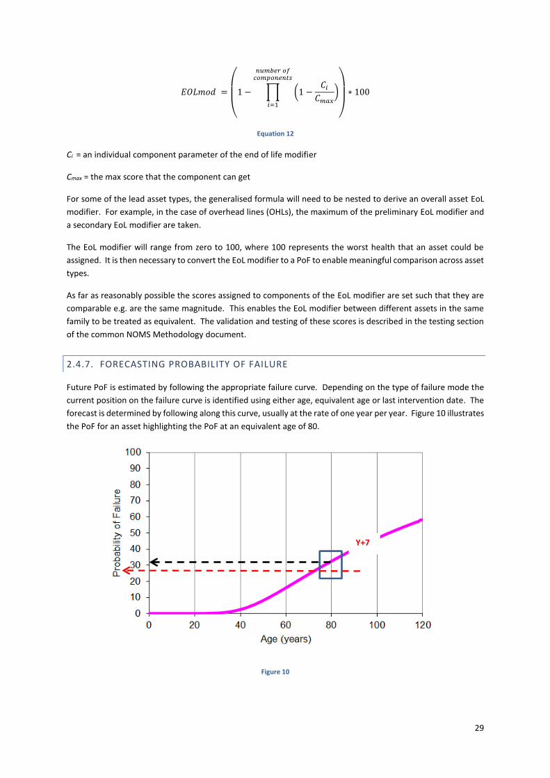
2.4.7. FORECASTING PROBABILITY OF FAILURE

Future PoF is estimated by following the appropriate failure curve. Depending on the type of failure mode the

current position on the failure curve is identified using either age, equivalent age or last intervention date. The

forecast is determined by following along this curve, usually at the rate of one year per year. Figure 10 illustrates

the PoF for an asset highlighting the PoF at an equivalent age of 80.

Figure 10

Y+7

30

The forecast probability of failure in future years can then be obtained by following along the curve. For example

the forecast for Y+7 would be the value given by the above curve at the equivalent age of 87. Note that in this

case it is not the real age of the asset, but an equivalent age that has been determined through the process

described in the above sections.

Where appropriate and enough historical data exists, a rate multiplier can be applied, so that for each annual

time step in forecast time equivalent age is increased or decreased by the rate multiplier time step. The default

value of the rate multiplier time step is set as 1.0 per year. This modelling feature will allow high duty assets to

be forecast more accurately.

2.4.8. HIGH LEVEL PROCESS FOR DETERMINING END OF LIFE PROBABILITY OF FAILURE

The process illustrated below will be used to determine the PoF of each asset. This is done by translating through

a probability mapping step, so that the appropriate end of life curve may be used to determine the probability

of an asset having failed.

Figure 11

This process is shown in more detail for each asset type in section 8 .

31

3. CONSEQUENCE OF FAILURE

The consequences of failure (CoF) may fall into four categories:

Consequence Description

System The impact on the network of the failure and any subsequent intervention required

Safety Impact of direct harm to public/personnel as a result of failure mode

Environment Impact of failure mode taking into account the sensitivity of the geographical area local to the asset

Financial Cost of the intervention needed to address and resolve the failure

Table 7

These categories reflect the impact of the various failure modes which are specific to the asset and the

consequences are consistent for each class of failure mode. The impact of the various failure modes will vary

depending on the type of failure. For example, for less disruptive failure modes there may be no impact from a

safety perspective.

Safety and environmental consequences are specific to the asset and its physical location.

In a highly-meshed system, such as a transmission network, consideration of system effects becomes

paramount. A comprehensive system of consequence evaluation must be derived, leading to a transparent,

objective and tradeable measure of risk.

In considering the safety and environment consequences, the concept of exposure is needed. Exposure is based

upon the asset’s location, i.e. its proximity to a location where it has the potential to cause harm (whether to

people or the environment).

Each consequence will be monetised and the price base for consequence of failure is defined in the NGET

Licensee Specific Appendix Section 3 – Consequence of Failure document.

NGET states which failure modes have been included in the analysis and explains why the chosen failure modes

are considered appropriate for the analysis.

It is the aim of this section to provide a quantified view in the terms of monetised consequence.

In taking the approach detailed below it is intended that the quantification forms an approximation to how this

may play out in the real world. In this case an approximation is of much greater value, due to its simplified nature

and the ease of comparison and benchmark. All quantities used will be externally verifiable and benchmarked,

where practicable to do so, as part of Calibration, Testing and Validation.

The monetisation does not correspond to the actual costs that will be incurred. The data used in the models

attempts to approach the correct orders of magnitude to avoid confusion it does not, however, guarantee this

and can only be treated as abstract.

3.1. SYSTEM CONSEQUENCE

The system consequence of a failure or failure mode effect of an asset is an indication of the asset’s importance

in terms of its function to the transmission system as given by the disruption to that function caused by the

failure. It is measured in terms of certain system related costs associated with system consequences incurred

by the industry electricity sector if that asset were to experience a failure. These system costs incurred due to

an asset failure can be divided into two categories, customer costs and System Operator costs. Regardless of

32

who initially pays these costs they are ultimately borne by electricity consumers. Customer costs are incurred as

a result of the disconnection of customers supplied directly or indirectly (via a distribution network) by the

transmission system. The cost for demand disconnections is expressed as the economic value that the user

assigns to that lost load. In the case of generators being disconnected from the network there is a mechanism

of direct compensation payments from the System Operator. The second category of costs are those that the

System Operator incurs in undertaking corrective and preventative measures to secure the system after asset

failures have occurred. These include generator constraint payments, response and reserve costs and auxiliary

services costs.

Unlike the environmental, financial and safety consequences of asset failures, the existence and scale of network

risk due to asset failures is dependent on the functional role that the failed asset plays in the transmission

system. The transmission system is designed with a degree of resilience that seeks to ensure the impact of asset

faults is contained within acceptable limits. It is the NETS SQSS that mandates a certain level of resilience that

the design and operation of the transmission system must meet when faced with a range of scenarios and

events. It is a license obligation of TOs that their networks comply with the NETS SQSS.

A range of negative system consequences (unacceptable overloading of primary transmission equipment,

unacceptable voltage conditions or system instability) must be avoided for ‘defined secured events’ under

certain network conditions. The required resilience is not absolute nor is it uniform across the network. The

philosophy behind the NETS SQSS is that lower severity consequences are to be accepted for relatively high

probability (and therefore high frequency) faults while more severe consequences are only to be accepted for

lower probability events. Figure 12 represents this philosophy.

This approach is further influenced by other considerations such as the geographical location of the assets in

question i.e. which TO License Area they are in, and for what timescales the network is being assessed (near

term operational timescales vs. long term planning timescales). The level of resilience required also varies

depending on the function of the part of the network in question. Parts of the network which connect demand,

generation or make up part of the Main Interconnected Transmission System (MITS) all have distinct design

requirements dependent upon their importance to the Transmission System and the total economic value of all

the customers they supply.

33

Allowed

Not Allowed

Severity of

Consequence

Probability of

Fault

Figure 12

Events that the NETS SQSS requires a degree of resilience against are described as ‘secured events’. These are

events that occur with sufficient frequency that it is economic to invest in transmission infrastructure to prevent

certain consequences when such events occur on the system. Secured events include faults on equipment and

these events range from single transmission circuit faults (highest frequency) to circuit breaker faults (lowest

frequency). When an asset fault occurs that results in the loss of only a single transmission circuit in an otherwise

intact network, almost no customer losses are permitted and all system parameters must stay within limits

without the SO taking immediate post-fault actions. While in the case of circuit breaker faults the NETS SQSS

only requires that the system is planned such that customer losses are contained to the level necessary to ensure

the system frequency stays within statutory limits to avoid total system collapse.

The key assumption that underpins this variation in permitted consequences of faults is that most faults are

weather related and that faults caused by the condition of the asset are rare. This can be seen in that faults on

overhead lines (often affected by wind and lightning) are relatively frequent events (≈20% probability per 100

km 400 kV circuit per annum) while switchgear faults are relatively less frequent (≈2% probability per 2-ended

400 kV circuit per annum). Another key assumption in the design of the SQSS is that faults are relatively short

in duration. A vast majority of circuits have a post-fault rating that is time limited to 24 hours, it is expected that

faults will be resolved within this time so that this rating will not be exceeded.

Asset failures driven by asset condition do not conform to these key assumptions, they occur in assets regardless

of their exposure to the elements and they can significantly exceed 24 hours in duration. The system therefore

cannot be assumed to be designed to be resilient against even a single asset failure. Even if system resilience is

sufficient to avoid an immediate customer or operator cost, no asset fault or failure that requires offline

intervention can be said to be free from a risk cost. At the very least, the unavailability of the asset reduces

system resilience to further events and therefore increases exposure to future costs.

34

3.1.1. QUANTIFYING THE SYSTEM RISK DUE TO ASSET FAULTS AND FAILURES

Fundamentally the transmission system performs three functions. It receives power from generators, transports

power where it is needed and delivers it to consumers. The system risk cost of a fault or failure can be quantified

by combining the following costs:

1. The economic value assigned to load not supplied to consumers including directly-connected demand

customers. Commonly described as Value of Lost Load (VOLL) in units of £/MWh

2. The cost of compensating generators disconnected from the transmission system, based on the market

cost of generation (£/MWh), the size of the generator (MW) and the expected duration of

disconnection (hours)

3. The cost of paying for other generators to replace the power lost from disconnected generation based

on the market cost of replacement generation (£/MWh) and number of megawatt hours that require

replacement

4. The increased cost in transporting power across the wider transmission network. This is comprised of:

a. Constraint payments to generators due to insufficient capacity in part of the transmission

system. This comprises the costs to constrain off generation affected by the insufficient

capacity and the cost to constrain on generation to replace it. If there is insufficient

replacement generation capacity, costs will include demand reduction.

b. Payments to generators to provide auxiliary services which ensure system security and quality

of supply e.g. the provision of reactive power.

The applicability and size of these cost sources are dependent upon the role of the failed asset in the system.

Some assets are solely for the connection of generation or demand, while others will provide multiple functions.

The methodology for calculating these potential costs is split into three parts:

1. A customer disconnection methodology, incorporating the cost of disconnecting generation, total

consumer demand and vital infrastructure sites (1, 2 and 3 above)

2. A boundary transfer methodology that estimates potential generator constraint payments (4a)

3. A reactive compensation methodology that estimates the cost of procuring reactive power to replace

that provided by faulted assets (4b)

Each of these methodologies will be described in turn in the following sections. All three share a common

structure that can be expressed by Equation 13.

𝐶𝑜𝑠𝑡 𝑜𝑓 𝑆𝑦𝑠𝑡𝑒𝑚 𝐼𝑚𝑝𝑎𝑐𝑡 = 𝑝𝑟𝑜𝑏𝑎𝑏𝑖𝑙𝑖𝑡𝑦 𝑥 𝑑𝑢𝑟𝑎𝑡𝑖𝑜𝑛 𝑥 𝑠𝑖𝑧𝑒 𝑥 𝑐𝑜𝑠𝑡 𝑝𝑒𝑟 𝑢𝑛𝑖𝑡

Equation 13

The total cost of system impact of a failure mode of an asset will be the sum of the consequence costs that come

from the three above costs.

35

3.1.2. CUSTOMER DISCONNECTION – CUSTOMER SITES AT RISK

With the exception of radial spurs, assets on the system will usually contribute towards the security of more

than one substation that connects customers to the network. However, the fewer other circuits that supply a

substation, the more important that asset is for the security of the site. In order to identify which sites are most

at risk of disconnection because of the failure of a specific asset, the number of circuits left supplying a customer

connection site after a failure of an asset, X, is defined;

𝑋 = 𝑛𝑢𝑚𝑏𝑒𝑟 𝑜𝑓 𝑝𝑎𝑟𝑎𝑙𝑙𝑒𝑙 𝑐𝑖𝑟𝑐𝑢𝑖𝑡𝑠 𝑠𝑢𝑝𝑝𝑙𝑦𝑖𝑛𝑔 𝑐𝑢𝑠𝑡𝑜𝑚𝑒𝑟 𝑠𝑖𝑡𝑒(𝑠)

− 𝑛𝑢𝑚𝑏𝑒𝑟 𝑜𝑓 𝑐𝑖𝑟𝑐𝑢𝑖𝑡𝑠 𝑡𝑟𝑖𝑝𝑝𝑒𝑑 𝑎𝑠 𝑎 𝑟𝑒𝑠𝑢𝑙𝑡 𝑜𝑓 𝑡ℎ𝑒 𝐹𝑎𝑖𝑙𝑢𝑟𝑒 𝑀𝑜𝑑𝑒 𝐸𝑓𝑓𝑒𝑐𝑡 𝑜𝑓 𝑡ℎ𝑒 𝑎𝑠𝑠𝑒𝑡

Equation 14

Circuit availability statistics indicate that the importance of a circuit decreases by around two orders of

magnitude for each extra parallel circuit available. Given that the uncertainty of other inputs into these

calculations will be greater than 1% it is a reasonable simplification to neglect all customer sites with values of

X greater than the minimum value of X; Xmin=min(X).

Once there are four or more circuits in parallel supplying a site additional circuits do not necessarily decrease

the probability of losing customers as the capacity of the remaining circuits will not be sufficient to meet the

import/export of the customers at risk. In parts of the network where the number and rating of circuits

connecting a substation are determined soley by the need to meet local demand, there is a significant risk that

once two or three circuits have been lost cascade tripping of remaining circuits due to overloading will result.

Therefore:

For assets on circuits containing transformers down to 132 kV or below if Xmin > 3 it will be treated as Xmin = 3 for

the purposes of calculating the Probability of Disconnection (Poc) and Duration (D).

Otherwise for assets on circuits at 275 kV or below if Xmin = 4 it will be treated as Xmin = 3 for the purposes of

calculating the Probability of Disconnection (Poc) and Duration (D).

Otherwise if Xmin > 3 then the risk of customer disconnection will be neglected as neglible.

As there will often be multiple customer connection sites with X=Xmin, to ensure that the methodology is efficient

and operable a variable Z, is introduced which is equal to the number of customer sites with X=Xmin for a given

asset. Only the largest group of customer sites that would be disconnected by the loss of a further Xmin circuits

is considered explicitly while the extra risk of customer disconnection due to other combinations of circuit losses

is approximated by the use of the risk multiplier coefficient MZ:

𝑀𝑍 =∑𝑍 + (𝑍 − 1) + (𝑍 − 2)+ . . .

𝑍

Equation 15

Intuitively M1 = 1, and MZ scales with increasing values of Z. Figure 13 illustrates an example of how MZ is

calculated with three customer sites (M3):

36

S1 S3S2

C1

C2

C3

C4

C5

C6

C7

C8

Figure 13

Three substations labelled S1, S2 and S3 are part of a double circuit ring with eight circuits labelled C1-C8. Each

substation is immediately connected to the rest of the system by four circuits and could be disconnected from

the system if these four immediate circuits were lost. However, each substation could also be disconnected by

other combinations of four circuit losses also. For example S2 could be disconnected by the loss of C3, C4, C5

and C6, but also by losing C3, C4, C7 and C8 or C1, C2, C5 and C6 etc. More than one substation would be lost

for these other combinations and all three substations would be lost for a loss of C1, C2, C7 and C8.

In order to calculate the total system consequence of a failure mode of an asset that is part of C1 we assume

that the volume and cost per unit of customer connections are approximately evenly distributed among the

substations (L for each substation) and that the probability (P) and duration (D) of each four circuit combination

being lost is approximately equal. The relative consequence of a loss event is then determined only by the

amount of customers lost. So a loss of S1 and S2 is twice the consequence of losing only S1. There is one

combination of four circuit losses involving C1 that disconnected a single substation, one combination that

disconnects two substations and one that disconnects all three. Therefore the risk cost is:

𝑅𝑖𝑠𝑘 𝑐𝑜𝑠𝑡 = (1×𝑃𝐷𝐿) + (1×2𝑃𝐷𝐿) + (1 ×3𝑃𝐷𝐿) = 6 𝑃𝐷𝐿

Equation 16

Given the risk cost of losing all three sites at once is 3PDL so the risk cost can be expressed as a function of the

risk cost of losing all three sites at once:

𝑅𝑖𝑠𝑘 𝑐𝑜𝑠𝑡 = 6 𝑃𝐷𝐿 = 2×3𝑃𝐷𝐿 = 3𝑃𝐷𝐿𝑀3

Equation 17

Therefore M3 is equal to 2.

3.1.3. CUSTOMER DISCONNECTION – PROBABILITY

The probability of a generator or consumer being disconnected as a consequence of an asset failure is a

function of a wide range of variables including the physical outcome of the failure , the local network topology,

asset composition of circuits, asset loading, physical proximity of assets, protection configuration and

operation options for restoration.. The probability of consequence is calculated as a function of five

probabilities, shown in Table 8.

Probability Symbol Determination of Value

Coincident outage Po TO statistics on planned unavailability of circuits

Damage to another circuit Pd TO historical experience of explosive/incendiary

failures of failure mode

Maloperation of another circuit Pm TO statistics on protection maloperation

Coincident fault to another circuit Pf TO fault statistics

Overloading of remaining circuit Pl TO specific network design

Table 8

37

The probabilities Po, Pd, Pm, Pf and Pl are determined separately by each TO according to their own methodology

outlined in TO specific appendices.

The probabilities in Table 8 can be combined to create a probability tree for each value of Xmin between 0 and 3.

Below are the resulting equations for Poc, the probability of disconnection.

For Xmin =0, Poc = 1

Equation 18

For Xmin = 1, Poc = 1 - NoNdNmNf

Equation 19

For Xmin = 2, Poc = Pd2 + 2PdNdPo + 2PdNdNoPm + 2PdNdNoNmPf + Nd

2PoPm + Nd2PoNmPf + Nd

2NoPmPf + Nd2NoNmPf

2

Equation 20

For Xmin = 3, Poc = Pd2Po + Pd

2NoPm + Pd2NoNmPf + Pd

2NoNmNfPl + 2PdNdPoPm + 2PdNdPoNmPf + 2PdNdPoNmNfPl +

2PdNdNoPmPf + 2PdNdNoPmNfPl + 2PdNdNoNmPf2 + 4PdNdNoNmPfNfPl + Nd

2PoPmPf + Nd2PoPmNfPl + Nd

2PoNmPf2 +

2Nd2PoNmPfNfPl + Nd

2NoPmPf2 + 2Nd

2NoPmPfNfPl + Nd2NoNmPf

3 + 3Nd2NoNmPf

2NfPl

Equation 21

Where No, Nd, Nm, Nf and Nl are the probabilities of no outage, no damage, no maloperation, no coincident faults

and no overloading respectively.

The derivation method of the above probability equations can be followed in Figures 14 & 15, the probability

tree diagram for the most complex of the four cases, Xmin = 3.

38

Initial pre-failure network state

Asset Experience

Failure Mode

3 circuits remaining

Probability of parallel outage

(Po)0 circuits remaining

(Pd2Po)

1 circuit remaining

Asset Failure damages asset on

two parallel circuits (Pd

2)

Probability of no parallel outage (No)

Probability of Maloperation

(Pm)

1 circuit remaining0 circuits remaining

(Pd2NoPm)

1 circuit remaining

Probability of no Maloperation (Nm)

1 circuit remaining

Probability of unrelated fault

(Pf)

0 circuits remaining(Pd

2NoNmPf)

Probability of no unrelated fault

(Nf)

Probability of overloading circuit (Pl)

0 circuits remaining(Pd

2NoNmNfPl)


Asset Failure damages asset on one parallel circuit

(2PdNd)

1 circuit remaining


(Pm)0 circuits remaining

(2PdNdPoPm)


(Po)


(2PdNdPoNmPf)



(Pf)


(Nf)


(2PdNdPoNmNfPl)





(Pm)

1 circuit remaining


(Pf)


(Nf)

1 circuit remaining

0 circuits remaining(2PdNdNoPmPf)


0 circuits remaining(2PdNdNoPmNfPl)


2 circuits remaining0 circuits remaining

(2PdNdNoNmPf2)

Probability of two unrelated faults

(Pf2)

Probability of no second unrelated

fault (2PfNf)

1 circuit remaining0 circuits remaining(4PdNdNoNmPfNfPl)


Asset Failure damages no assets on parallel circuits

(Nd2)

Continued Below

Figure 14

39



(Po)2 circuits remaining


(Pm)1 circuit remaining

0 circuits remaining(Nd

2PoPmPf)


(Pf)



(Nd2PoPmNfPl)

Probability of no unrelated fault (Nf)


Probability of no maloperation (Nm)

0 circuits remaining(Nd

2PoNmPf2)


(Pf2)


fault (2PfNf)


(2Nd2PoNmPfNfPl)





(Pm)


(Nd2NoPmPf

2)


(Pf2)


fault (2PfNf)


(2Nd2NoPmPfNfPl)


Probability of no maloperation (Nm)


(Nd2NoNmPf

3)

Probability of three unrelated

faults (Pf2)


(3PfPfNf)

1 circuit remaining0 circuits remaining(3Nd

2NoNmPf2NfPl)


Continued

Figure 15

40

3.1.4. CUSTOMER DISCONNECTION – DURATION

A similar approach is taken with the expected duration of such a disconnection event. This is dictated by the

failure mode of the asset in question, and both operational and asset interventions available to restore supply

to the customers. In order to calculate the duration of disconnection, six separate durations are introduced in

Table 9.

Duration Symbol Determination of Value

Duration of failure mode unavailability Dfm TO experience of failure durations

Outage restoration time Do TO statistics on planned unavailability of circuits

Circuit damage restoration time Dd TO historical experience of explosive/incendiary

failures of failure mode

Protection mal-operation restoration

time Dm TO statistics on protection maloperation

Unrelated fault restoration time Df TO fault statistics

Circuit overload restoration time Dl TO historical experience of overload trips

Table 9

The durations Dfm, Do, Dd, Dm and Df are determined separately by each TO according to their own

methodology outlined in TO specific appendices.The duration of customer loss is calculated by weighting the

probabilities of the event combinations outlined in the formulae for Poc and multiplying by the shortest of the

above durations that apply to that event combination. For example, if a failure mode with Xmin = 2 and

disconnection is due to a combination of the failure mode, a parallel outage and protection mal-operation

then the minimum of Dfm, Do and Dm is weighted with the other minimum durations of other disconnection

combinations. Below are the equations for D for different values of Xmin.

For Xmin = 0, D = Dfm

Equation 22

For Xmin = 1, D = [min(Dfm,Do)Po + min(Dfm,Dd)Pd + min(Dfm,Df)Pf + min(Dfm, Dm)Pm] / Poc

Equation 23

For Xmin = 2, D = [min(Dfm,Dd)Pd2 + min(Dfm, Dd, Do)2PdNdPo + min(Dfm,Dd,Dm)2PdNdNoPm +

min(Dfm,Dd,Df)2PdNdNoNmPf + min(Dfm,Do,Dm)Nd2PoPm + min(Dfm,Do,Df)Nd

2PoNmPf + min(Dfm,Dm,Df)Nd2NoPmPf +

min(Dfm,Df)Nd2NoNmPf

2] / Poc

Equation 24

For Xmin = 3, D = [min(Dfm,Dd,Do)Pd2Po + min(Dfm,Dd,Dm)Pd

2NoPm + min(Dfm,Dd,Df)Pd2NoNmPf +

min(Dfm,Dd,Dl)Pd2NoNmNfPl + min(Dfm,Dd,Do,Dm)2PdNdPoPm + min(Dfm,Dd,Do,Df)2PdNdPoNmPf +

min(Dfm,Dd,Do,Dl)2PdNdPoNmNfPl + min(Dfm,Dd,Dm,Df)2PdNdNoPmPf + min(Dfm,Dd,Dm,Dl)2PdNdNoPmNfPl +

min(Dfm,Dd,Df)2PdNdNoNmPf2 + min(Dfm,Dd,Df,Dl)4PdNdNoNmPfNfPl + min(Dfm,Do,Dm,Df)Nd

2PoPmPf +

min(Dfm,Do,Dm,Dl)Nd2PoPmNfPl + min(Dfm,Do,Df)Nd

2PoNmPf2 + min(Dfm,Do,Df,Dl)2Nd

2PoNmPfNfPl +

min(Dfm,Dm,Df)Nd2NoPmPf

2 + min(Dfm,Dm,Df,Dl)2Nd2NoPmPfNfPl + min(Dfm,Df)Nd

2NoNmPf3 +

min(Dfm,Df,Dl)3Nd2NoNmPf

2NfPl ]/ Poc

Equation 25

41

3.1.5. CUSTOMER DISCONNECTION – SIZE AND UNIT COST

Once the largest group of customer sites with X = Xmin for a given failure mode of an asset has been identified

the size of consequence of disconnection of this group must be fully quantified. The weighted quantity of

generation disconnected, MWW is given by:

𝑀𝑊𝑊 =∑𝜑𝑀𝑊𝐺𝑇𝐸𝐶

Equation 26

Where MWGTEC is the Transmission Entry Capacity (TEC) of each disconnected generator and φ is the design

variation weighting factor. This factor equals 1 for generators who are connected with standard SQSS levels of

security. Its value for generators with lower than standard levels of security will be determined by each TO. TEC

is used without any reference to load factor as this is how generator disconnection compensation is calculated

as laid out in the Connection and Use of System Code (CUSC). Secondly the annual average true demand of

customers disconnected, MWD, is calculated by summing the peak demand and the embedded generation

contribution during peak of all sites at risk. Both the peak demand and contribution of embedded generation is

taken directly from DNO week 24 data submissions. The final inputs are the number of vital infrastructure sites

of three different types supplied by sites at risk as shown in Table 10. These are demand sites of particular

importance in terms of economic or public safety impact. There is no additional quantification of the risk of

disconnection of customers or consumers for which the disconnection risks are considered High Impact Low

Probability (HILP) events. The risk is treated on a per MW basis like any other consumer or customer.

The lists of sites that belong to the categories outlined in Table 10 are deemed sensitive and thus are not included

here. The selection criteria and sources for the lists of sites can be found in the individual TO specific appendices.

The costs of disconnection per site, per hour were calculated by collecting as much publicly available information

as possible on the costs of historic disconnection events of comparable infrastructure sites across the developed

world. These costs per minute or per event were converted into current sterling prices through exchange rate

and price indexation conversion. An average for each category was then taken.

Vital Infrastructure Category

Symbol and Cost

Number of

Sites

Cost per site per hour

(£/hr)

Cost per site per disconnection event (£)

Transport Hubs ST VT -

Economic Key Point SE VE -

Particularly sensitive COMAH sites SC - VC

Table 10

The values for VT, VE and VC are contained within the NGET Licensee Specific Appendices.

The final component of the risk cost, the per unit cost, is separately defined for the three above quantities of

customer loss. VOLL in £/MWh is the same RPI indexed value as that used in the RIIO-T1 energy not supplied

incentive (see NGET Licensee Specifc Appendix for value)

The cost of disconnection of generation is in two parts, firstly the generation compensation payment cost, GC,

in £/MWh varies with outage duration is based upon the CUSC methodology and uses cost information from

System Operator.

For D ≤ 1.5h, 𝐺𝑐 = 𝑀𝑊𝑊𝐷𝐶𝑆𝐵𝑃

Equation 27

42

For 1.5 h < D ≤ 24h, 𝐺𝑐 = 𝑀𝑊𝑊(1.5𝐶𝑆𝐵𝑃 + {𝐷 − 1.5}𝐶𝑆𝑀𝑃)

Equation 28

For D > 24h, 𝐺𝑐 = 𝑀𝑊𝑊(1.5𝐶𝑆𝐵𝑃 + 22.5𝐶𝑆𝑀𝑃 + {𝐷 − 24}𝐶𝑇𝑁𝑈𝑜𝑆)

Equation 29

Where CSBP is the annual average system buy price in £MWh-1, CSMP is the annual average system marginal price

in £MWh-1 and CTNUoS is the average Transmission Network Use of System (TNUoS) refund cost per MW per hour.

CTNUoS is calculated by divided the annual TNUoS charge for all generators by the total of TEC of all generators

and again by 8760.

Secondly, the cost of generation replacement, GR*, again dependent on D is defined as below.

For D ≤ 2h, 𝐺𝑅 = 𝐷𝐶𝑆𝑀𝑃(0.42𝑀𝑊𝑊 − 0.62𝑀𝑊𝐷)

Equation 30

For D > 2h, 𝐺𝑅 = 2𝐶𝑆𝑀𝑃(0.42𝑀𝑊𝑊 − 0.62𝑀𝑊𝐷)

Equation 31

For GR ≥ 0, GR* = GR

Equation 32

For GR < 0, GR* = 0

Equation 33

This cost reflects the expense of the System Operator constraining on generation to replace that lost by the

disconnection of generation. The equation multiples the duration of the disconnection and the annual average

price to constrain on plant by the mismatch between the expected mismatch between generation and demand

disconnected by the event. This mismatch is calculated by first taking the total TEC of generation connected to

the customer sites in the group at risk, MWW, and multiplying it by the system wide average generation load

factor 0.42 (calculated by dividing the total energy generated in a year in MWh across the whole system by 8760

and then by the total TEC of all generation on the system). Secondly the peak adjusted demand, MWD, of all

customer sites in the group is multiplied by the average demand factor 0.62 (calculated by dividing the total

annual transmission demand in MWh by 8760 and dividing again by the winter peak demand in MW). The

difference between these two numbers is the mismatch, multiplied by the System Marginal Price in £MWh-1 and

the duration up to a maximum of 2 hours. After 2 hours it would be expected that the market would have self-

corrected for the generation mismatch.

The vital infrastructure site disconnection cost, V, is the numbers of different types of vital infrastructure sites

multiplied by the cost per site and in the case of transport and economic key point sites multiplied by D.

𝑉 = 𝐷(𝑉𝑇𝑆𝑇+𝑉𝐸𝑆𝐸) + 𝑉𝐶𝑆𝐶)

Equation 34

With all elements of the equation defined, the customer disconnection risk cost, Rcustomer, of a given asset failure

mode of any asset can be defined by Equation 35.

43

𝑅𝑐𝑢𝑠𝑡𝑜𝑚𝑒𝑟 = 𝑃𝑜𝑐[𝐺𝐶 + 𝐺𝑅 + 0.62𝐷𝑀𝑊𝐷𝑉𝑂𝐿𝐿 + 𝑉]𝑀𝑧

Equation 35

A vast majority of lead assets will return a non-zero value for customer disconnection risk, the exceptions being

shunt reactors and circuits which connect nodes with more than 4 circuits. These assets will have material risks

for one of the next two elements of system consequence.

Note that in the future it may be possible to vary VOLL with the type of load lost but this is not included in the

current methodology.

3.1.6. BOUNDARY TRANSFER

This methodology estimates the cost impact of having to pay generation constraint payments in order to restrict

flows across a system boundary. Unlike the customer disconnection methodology, there is not a discrete

disconnection event that either occurs or doesn’t (within a given probability) but instead there is a year-round

average cost per hour at which the boundary must be constrained which implicitly includes the probability of a

constraint existing. The constraint cost per hour is dependent upon the number of circuits unavailable by the

asset failure, Y. In the vast majority of cases this will be 1, but tower failures would usually result in two circuits

being lost until the asset can be restored. Additionally the extra constraint cost that would result from unrelated

unavailability on another circuit on the same boundary must be considered.

The derivation of average constraint costs will be based on flow and price information provided by the System

Operator on an annual basis. The System Operator will run simulations of a full year of operation with each

boundary in with intact, N-1 depletion, N-2 depletion and N-3 depletion capabilities resulting in four annual costs

of operation for the boundary, BY,which is then calculated as follows:

𝐵1 =[(𝑎𝑛𝑛𝑢𝑎𝑙 𝑛 − 1 𝑐𝑜𝑠𝑡) − (𝑎𝑛𝑛𝑢𝑎𝑙 𝑖𝑛𝑡𝑎𝑐𝑡 𝑐𝑜𝑠𝑡)]

8760

Equation 36


8760

Equation 37


8760

Equation 38

While a failure mode that renders Y circuits unavailable will incur costs at least the BY level, on average a

proportion of the duration of the failure mode will be spent with Y+1 circuits unavailable, defined as PY+1. The

proportion used is derived from historic fault and outage probabilities and durations. The probability of

sustained boundary depletion beyond Y+1 circuits is assumed to be negligible.

These costs are multiplied by the duration of the unavailability of the asset until it is returned to service, Dfm,

dependent upon historic precedent for the asset type and failure mode in question.

With the variables defined the methodology for determining the boundary transfer risk cost, Rboundary, of an asset

failure mode of any asset can be described by Equation 39.

44

𝑅𝑏𝑜𝑢𝑛𝑑𝑎𝑟𝑦 = 𝐷𝑓𝑚[𝐵𝑌(1 − 𝑃𝑌+1) + 𝐵𝑌+1𝑃𝑌+1]

Equation 39

This methodology will return non-zero risk costs for all assets that belong to or affect circuits critical to the

capability of one or more system boundaries with significant constraint implications.

Equation 39 can be illustrated with the example of B6, the boundary between the SPT and National Grid

Electricity Transmission (NGET) areas. There are currently four circuits that make up this boundary. If a failure

of an asset which makes up part of one of these circuits occurs then this circuit will be unavailable until the

failure has been rectified, Y = 1 for this failure. The boundary will be at N-1 depletion until the failure is rectified

and on average will spend some proportion, PY+1, of the duration of failure at a N-2 depletion level due to

unrelated prior outages or other unrelated faults. The weighted average boundary constraint cost per hour is

calculated by first multiplying B1 by (1- PY+1), the proportion of time that the boundary is at N-1 depletion. Then

B2 is multiplied by the proportion of time that the boundary will spend at N-2 depletion, PY+1. These two

products are added together. This average boundary cost per hour is then simply multiplied by the average time

taken to restore the circuits to service by repairing the failed asset, Dfm. This gives us the total expected

boundary constraint for the failure mode of the asset.

3.1.7. REACTIVE COMPENSATION

The third methodology calculates the cost impact of having reactive compensation unavailable due to a fault or

failure of any asset that would render the reactive compensation unusable. This could include circuit breakers,

transformers and cables as well as the compensation itself. The purpose of reactive compensation is to produce

or consume reactive power to aid control of system voltage. When compensation equipment is unavailable this

reactive power control is either procured from generators instead or elements of the transmission system are

de-energised, reducing system resilience. As a simplification the cost impact of a fault or failure can be

quantified as the volume of reactive power not supplied multiplied by the cost per MVArh the SO must pay to

buy the same service from generators. Therefore we have Equation 40Equation 39 to calculate the reactive

compensation system risk cost, RRC, of an asset Failure Mode:

𝑅𝑅𝐶 = 𝑅𝐹𝐷𝑓𝑚𝑄𝐶𝑀𝑉𝐴𝑟ℎ

Equation 40

RF is the requirement factor of the compensation equipment made unavailable or the proportion of the year

that the compensation in question is required on a scale of 0 to 1. Dfm is the duration of unavailability due to

the asset failure mode. Q is the capacity of the asset in MVAr and CMVArh is the average cost of procuring of MVAr

from generation sources.

CMVArh will be calculated by taking an annual sum of all costs of generators to absorb MVArs including BM actions

to bring plant into service and constrain others as well as the cost of providing the reactive absorption itself.

This sum is divided by the total number of MVArhs that were absorbed by generators over the year.

3.2. SAFETY CONSEQUENCE

When assets fail they have the potential to cause harm to both the general public and personnel who work on

or near to the assets. In circumstances where this happens, there is a cost to society as a whole. The aim of this

part of the methodology is therefore to capture the safety risks that deteriorating assets present to individuals

who are exposed to their effects and the associated cost. In general the safety risk for an individual asset can be

expressed as shown below:

45

𝑆𝑎𝑓𝑒𝑡𝑦 𝑅𝑖𝑠𝑘 =∑(𝑃(𝐶𝑠𝑎𝑓,𝑖) × 𝐶𝑠𝑎𝑓,𝑖)

𝑖

Equation 41

Where:

𝑃(𝐶𝑠𝑎𝑓,𝑖) = Probability of failure mode effect i occurring as a result of a failure event

𝐶𝑠𝑎𝑓,𝑖 = Safety-related costs associated with asset failure resulting in failure mode effect i

For an individual asset the general expression for 𝐶𝑠𝑎𝑓 is as follows:

𝐶𝑠𝑎𝑓 = 𝑃𝑟𝑜𝑏𝑎𝑏𝑖𝑙𝑖𝑡𝑦 𝑜𝑓 𝐼𝑛𝑗𝑢𝑟𝑦 ×𝐶𝑜𝑠𝑡 𝑜𝑓 𝐼𝑛𝑗𝑢𝑟𝑦 ×𝑆𝑎𝑓𝑒𝑡𝑦 𝐸𝑥𝑝𝑜𝑠𝑢𝑟𝑒

Equation 42

Where:

Probability of Injury – the likelihood that an individual is injured when exposed to the effects of an asset failure

Cost of Injury – the cost associated with an individual sustaining an injury

Safety Exposure – modifier to reflect the number of people who are exposed to the effects of an asset failure

In reality, individuals exposed to asset failures can potentially sustain injuries of varying severity and the

likelihood of these injuries occurring will depend on the asset under consideration, the type of failure that occurs

and the effects associated with that failure. Moreover, the cost associated with different types of injury will

vary. Taking into account these variables the ‘Safety Cost’ can be more formally expressed as shown below:

𝐶𝑠𝑎𝑓,𝑖 =∑𝑃𝑟𝑜𝑏𝑎𝑏𝑖𝑙𝑖𝑡𝑦 𝑜𝑓 𝐼𝑛𝑗𝑢𝑟𝑦𝑗,𝑖 ×𝐶𝑜𝑠𝑡 𝑜𝑓 𝑖𝑛𝑗𝑢𝑟𝑦𝑗 × 𝑆𝑎𝑓𝑒𝑡𝑦 𝐸𝑥𝑝𝑜𝑠𝑢𝑟𝑒

𝑗

Equation 43

Where:

i

j

=

=

Failure Mode Effect

Injury Type

3.2.1. FAILURE MODE EFFECT & PROBABILITY OF FAILURE MODE EFFECT

The failure mode effect represents the possible effects that NGET considers as a result of failure and the

probability of failure mode effect represents its likelihood of occurrence. The effects that are considered by

NGET and the calculation of their likelihood are described below.

46

3.2.2. INJURY TYPE & PROBABILITY OF INJURY

Individuals can sustain varying degrees of injury as a result of an asset failure. NGET proposes to categorise the

severity of injury into the following types, using HSE definitions2:

1. Slight – Injury involving minor cuts and bruises with a quick and complete recovery

2. Serious - Slight to moderate pain for 2-7 days. Thereafter some pain/discomfort for several weeks.

Some restrictions to work and/or leisure activities for several weeks/months. After 3-4 months return

to normal health with no permanent disability.

3. Permanent Incapacitating Injury - Moderate to severe pain for 1-4 weeks. Thereafter some pain

gradually reducing but may recur when taking part in some activities. Some permanent restrictions to

leisure and possibly some work activities.

4. Fatality

The ‘Probability of Injury’ represents the likelihood that an individual is injured when exposed to the effects of

an asset failure. Probabilities will be assigned to each ‘Injury Type’ considered. The probability assigned to each

category will vary depending on the failure mode that occurs and the effects that occur as a result of the failure

mode effect materialising. For less disruptive failures there may be no impact from a safety perspective and the

probability of injury will be zero. In addition, because it is assumed that the probability of injury applies to an

individual, the sum of probabilities across all injury types categories for a particular failure effect is less than or

equal to unity (i.e. an individual’s injuries can only be classified under a single category of injury).

3.2.2.1. COST OF INJURY

Fixed costs will be assigned to the different injury types recognised by the HSE as per their website3, which are

inflated to a cost-base of 2016/17 in line with RPI4.

Whilst the appraisal values reflect a broad range of cost categories, for simplicity of presentation the appraisal

values can be divided into two main component costs:

• Human costs - representing a monetary estimate of the loss of quality of life, and loss of life in the case

of fatal injuries

• Financial costs, which are the sum of the following:

o Productivity costs including:

▪ net lost income, taking into account of loss of output and earnings due to absence

from work, and offsetting transfers from one party to another, e.g. benefits payments

are a cost to Government, but an equal and opposite offsetting benefit to individuals

▪ production costs, such as cost of recruitment and work reorganisation

o The cost of Employer’s Liability Compulsory Insurance, less compensation payouts to

individuals

o Health and rehabilitation costs, such as NHS costs

o Administrative and legal costs, such as costs of administering benefits claims

2 http://www.hse.gov.uk/risk/theory/alarpcheck.htm 3 http://www.hse.gov.uk/risk/theory/alarpcheck.htm 4 https://www.ons.gov.uk/economy/inflationandpriceindices/timeseries/chaw/mm23

47

Each of these factors is discussed in the following sections. NGET anticipates that the ‘Cost of Injury’ will be

calculated as below:

𝐶𝑜𝑠𝑡 𝑜𝑓 𝐼𝑛𝑗𝑢𝑟𝑦𝑗 =∑𝑇𝑜𝑡𝑎𝑙 𝐶𝑜𝑠𝑡 (𝑅𝑜𝑢𝑛𝑑𝑒𝑑)×𝐷𝑖𝑠𝑝𝑟𝑜𝑝𝑜𝑟𝑡𝑖𝑜𝑛 𝐹𝑎𝑐𝑡𝑜𝑟

Equation 44

The ‘Total Cost (Rounded)’ is reflected by the HSE values, as per their website, which are inflated to a cost-base of 2016/17 in line with RPI. A disproportion factor recognises the high risk nature of the Transmission Industry. Such disproportion factors are described by the HSE guidance when identifying reasonably practicable costs of mitigation. This value is not mandated by the HSE but they state that they believe that “the greater the risk, the more should be spent in reducing it, and the greater the bias should be on the side of safety”5.

The value of the disproportion factor is included in each Licensee Specific Appendix, as the disproportion factor

reflects the organisation’s risk appetite.

3.2.3. SAFETY EXPOSURE

Safety consequences are specific to individual assets and their physical location. Some assets will expose a

greater number of people to their failure effects than others depending on the levels of activity near to the asset.

The ‘Probability of Injury’ only considers whether an individual will be injured assuming they are exposed to the

effects of an asset failure and does not consider whether it is likely that one or more individuals will be within

the vicinity of an asset when it fails. In order to take into account the likely number of people exposed to the

effects of an asset failure (e.g. where an event impacts multiple people at the same time) a ‘Safety Exposure’

modifier is incorporated into the ‘Safety Cost of Failure Mode Effects’ calculation.

Under the Electricity Safety Quality and Continuity Regulations 2002 (ESQCR), risk assessments must be carried

out on NGET assets to assess the risk of interference, vandalism or unauthorised access to the asset by the

public.

The overall safety exposure value is built from the following components:

• Location:

o Proximity to areas that may affect its likelihood of trespass or interference

o Personnel activity in the vicinity of the asset

Location/Exposure Risk Rating

Low Limited personnel access. No likely public access

Medium Regular personnel/public activity in the vicinity of the asset

High High levels of personnel/public activity in the vicinity of the asset

Very High Constant personnel/public activity in the vicinity of the asset

Table 11

The values used for each safety exposure score (Low-Very High), are included in the Licensee Specific Appendix.

The following factors have been taken into consideration:

5 http://www.hse.gov.uk/risk/theory/alarpcheck.htm

48

• Number of hours per annum of an individual staff member being in the vicinity of an asset on the

system, due to:

o Routine activities

o Maintenance activities

o Replacement activities

o Switching activities

o Meetings in substation buildings

o Office base at substation buildings

• Number of hours per annum to an individual member of the public being in the vicinity of an asset,

due to:

o Domestic activity

o Industrial activity

o Rights-of-way

o Agricultural activity

o Educational activity

o Commercial activity

o Retail activity

The safety exposure factor takes an average value of hours per annum for an individual to be within the vicinity

of an NGET asset. This presents an average safety exposure value for each of the four categories, reflective of a

ratio of the number of hours per annum for an individual to be within the vicinity of an NGET asset compared to

the number of hours in a year. The average value is taken due to the number of NGET sites, such that the sites

included in each exposure category can vary significantly, and the category for ‘Very High’ exposure will contain

the anomaly sites with extreme cases of public and staff exposure, significantly higher than the remaining sites

within that category. The average value is used as the most appropriate representation of the exposure levels

for the majority of sites within each relevant exposure category.

3.3. ENVIRONMENTAL CONSEQUENCE

When assets fail they have the potential to impact on the geographical area local to the asset. The aim of this

part of the methodology is to capture the different environmental effects that deteriorating assets present and

the associated costs. In general the total environmental risk for an asset can be expressed as shown below:

𝐸𝑛𝑣𝑖𝑟𝑜𝑛𝑚𝑒𝑛𝑡𝑎𝑙 𝑅𝑖𝑠𝑘 =∑(𝑃(𝐶𝑒𝑛𝑣,𝑖) ×𝐶𝑒𝑛𝑣,𝑖)

𝑖

Equation 45

Where:

𝑃(𝐶𝑒𝑛𝑣,𝑖) = Probability of failure mode effect i occurring as a result of a failure event

𝐶𝑒𝑛𝑣,𝑖 = Environmental-related costs associated with asset failure resulting in failure mode effect i

For an individual asset the general expression for 𝐶𝑒𝑛𝑣 is:

49

𝐶𝑒𝑛𝑣 = 𝑃𝑟𝑜𝑏𝑎𝑏𝑖𝑙𝑖𝑡𝑦 𝑜𝑓 𝐸𝑛𝑣𝑖𝑟𝑜𝑛𝑚𝑒𝑛𝑡𝑎𝑙 𝐼𝑚𝑝𝑎𝑐𝑡×𝐶𝑜𝑠𝑡 𝑜𝑓 𝐸𝑛𝑣𝑖𝑟𝑜𝑛𝑚𝑒𝑛𝑡𝑎𝑙 𝐼𝑚𝑝𝑎𝑐𝑡 ×𝐸𝑛𝑣𝑖𝑟𝑜𝑛𝑚𝑒𝑛𝑡𝑎𝑙 𝐸𝑥𝑝𝑜𝑠𝑢𝑟𝑒

Equation 46

Where:

Probability of Environmental Impact – the likelihood that there is an environmental impact as a result of a

particular asset failure mode effect

Cost of Environmental Impact – the costs arising from a failure event that has an impact on the environment

Environmental Exposure – modifier to reflect the sensitivity of the environment exposed to the effects of an

asset failure event

In reality, the environment exposed to asset failures can potentially sustain varying severities of environmental

impacts, and the likelihoods of these environmental impacts occurring is dependent on the asset under

consideration, the type of failure that occurs and the effects associated with the failure. Consequently, the costs

associated with different types of environmental impacts will vary. Taking into account these variables the

‘Environmental Cost of Failure Mode Effect’ can be formally expressed as shown below:

𝐶𝑒𝑛𝑣,𝑖 =∑ 𝑃𝑟𝑜𝑏𝑎𝑏𝑖𝑙𝑖𝑡𝑦 𝑜𝑓 𝐸𝑛𝑣𝑖𝑟𝑜𝑛𝑚𝑒𝑛𝑡𝑎𝑙 𝐼𝑚𝑝𝑎𝑐𝑡𝑗,𝑖 ×𝐶𝑜𝑠𝑡 𝑜𝑓 𝐸𝑛𝑣𝑖𝑟𝑜𝑛𝑚𝑒𝑛𝑡𝑎𝑙 𝐼𝑚𝑝𝑎𝑐𝑡

𝑗 ×𝐸𝑛𝑣𝑖𝑟𝑜𝑛𝑚𝑒𝑛𝑡𝑎𝑙 𝐸𝑥𝑝𝑜𝑠𝑢𝑟𝑒

𝑗

Equation 47

Where:

i = Failure Mode Effect

j = Environmental Impact Type

3.3.1. FAILURE MODE EFFECT & PROBABILITY OF FAILURE MODE EFFECT

The failure mode effects represent the possible effects that NGET considers as a result of a failure event and the

probability of failure mode effect represents its likelihood of occurrence. The environmental effects that are

considered by NGET and the calculation of their likelihoods are described below.

The probability assigned to each environmental impact type, see section 1.1.2, will vary depending on the failure

mode that occurs and the effects that result from the failure mode event materialising. For less disruptive

failures there may be no impact on the environment, and the probability of environmental impact would then

be zero. In addition, because it is assumed that the probability of impact applies to an individual site, the sum

of probabilities across all impact type categories for a particular failure effect is less than or equal to unity (i.e.

the environmental impact that occurs at a site can only be classified under a single impact type).

3.3.2. ENVIRONMENTAL IMPACT TYPE

The severity of the environmental impact, as a result of an asset failure can vary. NGET proposes to categorise

the severity of different environmental impact types, by the following table:

50

Impact Type Environmental Impact

• Near Miss - An incident, which under different circumstances had the

potential to cause harm or damage to the environment

Low

• Events resulting in environmental harm or damage

• Prosecution or enforcement action by a regulatory body or adverse

public perception is deemed unlikely

Moderate

• Significant environmental harm or damage, incidents which are

significant to us as a business and drive different decisions and/or

behaviours.

• National Grid receiving formal written notification of enforcement

action from a regulatory authority

• Regulators and similar bodies taking an active involvement in our

activities as a result of the incident

Significant

Table 12

3.3.2.1. COST OF ENVIRONMENTAL IMPACT

Costs will be assigned to the different environmental impact types, as detailed in the Licensee Specific

Appendix. These include:

• Environmental cost per litre of oil

• Environmental cost per kg of SF6 lost This is derived from:

o Traded carbon price

o Cost of SF6 loss compared with the cost of carbon

• Environmental cost of fire

• Environmental cost per tonne of waste

The values are provided in the Licensee Specific Appendix.

3.3.3. ENVIRONMENTAL EXPOSURE

Due to the distributed nature of networks it is important that exposure is taken into account. Environmental

consequences are specific to individual asset size and their physical location. Some assets pose a greater risk to

the environment than others. In order to account for this an ‘Environmental Exposure’ modifier is incorporated

into the ‘Environmental Consequence of Failure Mode Effect’ calculation. The environmental exposure values

are included in the Licensee Specific Appendix.

3.3.3.1. LOCATION FACTOR

Location factor allows for an adjustment to be made based on an assessment of the environmental sensitivity

of the site on which an asset is located. The specific concerns will vary by asset type but include proximity to

watercourses and other environmentally sensitive areas. The factor also recognises any mitigation associated

with the asset. This factor is derived by combining separate factors relating to proximity to a watercourse or

Site of Special Scientific Interest (SSSI).

Environmental Exposure Category Criteria

51

Low • Asset located in controlled environment

Medium • Asset may be located in controlled, environment which may be located within 100m of environmentally sensitive area.

• Distributed asset located greater than 100m from sensitive environment

High • Distributed asset, all or part of which, is located within 100m of Source Protection Zone, abstraction or surface water course or SSSI

Table 13

3.4. FINANCIAL CONSEQUENCE

The Financial Consequence of Failure is derived from an assessment of the typical replacement and repair costs

incurred by the failure of the asset in each of its applicable Failure Modes and is multiplied by the probability of

each Failure Mode effect.

𝐹𝑖𝑛𝑎𝑛𝑐𝑖𝑎𝑙 𝑅𝑖𝑠𝑘 (𝑘) = ∑(𝑃(𝐶𝑓𝑖𝑛,𝑖) ×𝐶𝑓𝑖𝑛,𝑖)

𝑖

Equation 48

Where:

𝑃(𝐶𝑓𝑖𝑛,𝑖) = Probability that event i occurs

𝐶𝑓𝑖𝑛,𝑖 = Financial consequence of the event’s effect

The FMEA process identifies asset items and the failure events associated with them. Each failure event may

result in one or more Failure Mode effects and each effect has consequences. The probability of the events

resulting from each Failure Mode is determined through the FMEA process.

The Financial Consequence for each effect is derived from the average cost to repair or replace the asset (or

assets, if the failure results in a disruptive failure where adjacent assets are damaged) based on existing repair

and replacement data. The costs presented are the labour and repair costs as well as OMGS (Other Materials,

Goods and Services), which are necessary to carry out the repair or replacement of the failed asset. Additional

costs, associated with the failure but not incurred in carrying out the repair or replacement, such as

environmental clean-up or formal incident investigation costs (undertaken following catastrophic failures, for

example), are not considered as part of the Financial Consequence.

To illustrate, the following Failure Mode effects result from events associated with transformers. It is the event

which has the consequence; hence the costings are derived for each event. In order to validate the costing, the

Failure Modes which cause the event are also presented.

52

Event Connected with Failure Mode/cause

Activities used to derive average cost (this table will show actual costs in the Licensee Specific Appendix following CTV)

01- No Event

02- Environment Noise Noise caused by anti vibration pads failing or faulty fans

Labour costs and component costs plus OMGS

03- Reduced Capability Downratings due to pumps/fans failure or overheating caused by carbon build up on tap changers

Labour costs to investigate and repair. Component costs + OMGS

04- Alarm Overheating alarm Labour costs for alarm investigation

05- Unwanted Alarm + Trip

Unintentional operation of Buchholz or WTI Labour costs for trip investigation

06- Transformer Trip high res contacts on diverters Labour costs for trip investigation

07- Reduced Capability + Alarm + Trip

Overheating due to WTI failure Contactor/control relay failure Pump failure Fan failure Incorrect valve position Blockages (sludging) cooler blockage external OR loss of oil due to tank corrosion


08- Fail to Operate + Repair

Buchholz or WTI fail to trip or alarm, overheating on tap changers,


09- Reduced Capability + Alarm + Loss of Voltage Control + Fail to Operate

Tap changer motor drive defects Labour costs to investigate and repair. Component costs + OMGS

10- Overheating (will trip on overload)

Overheating due to carbon build up or high resistance contacts in tap changer or overheating due to WTI failure Contactor/control relay failure Pump failure Fan failure Incorrect valve position Blockages (sludging) cooler blockage external


11- Cross Contamination of Oil

Gasket leak, drive seal failure, corrosion on diverters


12- Alarm + Damaged Component (Tap Changer) No Trip

Diverter mechanism jams due to loose permali nuts

Labour costs to investigate and repair. Component costs + OMGS. May necessitate replacement of tap changer.

13- Alarm + Trip + Damaged Component (Tap Changer)

Selector/diverter fail to complete op or flashover. Diverter open circuit, loss of containment

Labour costs to investigate and repair. Component costs + OMGS. May necessitate replacement of tap changer.

53

14- Alarm + Trip + Transformer Internal Damage

Selector/diverter fail to complete operation or flashover. Diverter go open circuit, loss of containment - but in this case the transformer is damaged not just the tap changer

Labour costs to investigate and repair. Component costs + OMGS. Significant damage to the transformer windings.

15- loss of oil into secondary containment

Major oil leak, tank breach Labour costs to investigate and repair. Component costs + OMGS.

16- Alarm + Trip + Damage + State Requiring Replacement (Asset Replacement)

End of Life owing to deterioration

Unit cost for replacement of the asset

17- Alarm + Trip + Disruptive Failure + External Damage (danger) + Replacement

Disruptive failure - potential for bushing porcelain projectiles

Replacement of the asset plus costs of replacing/repairing any adjacent assets damaged

18- Alarm + Trip + Disruptive Failure + External Damage (danger) + Replacement+ Transformer Fire

Transformer fire

Replacement of the asset plus costs of replacing/repairing any adjacent assets damaged by the fire

Table 14

54

4. RISK

4.1. METHODOLOGY FOR CALCULATION OF RISK

As stated in section 1.3.7, for a given asset (k), a measure of the risk associated with it is the Asset Risk (Ak), given

by:

𝐴𝑠𝑠𝑒𝑡 𝑅𝑖𝑠𝑘(𝐴𝑘) = ∑𝑃(𝐶𝑗)

𝑛

𝑗=1

× 𝐶𝑗

Equation 49


𝑃(𝐶𝑗) = 𝑃𝑟𝑜𝑏𝑎𝑏𝑖𝑙𝑖𝑡𝑦 𝑜𝑓 𝑐𝑜𝑛𝑠𝑒𝑞𝑢𝑒𝑛𝑐𝑒 j 𝑜𝑐𝑐𝑢𝑟𝑟𝑖𝑛𝑔 𝑑𝑢𝑟𝑖𝑛𝑔 𝑎 𝑔𝑖𝑣𝑒𝑛 𝑡𝑖𝑚𝑒 𝑝𝑒𝑟𝑖𝑜𝑑

𝐶𝑗 = 𝑡ℎ𝑒 𝑚𝑜𝑛𝑒𝑡𝑖𝑠𝑒𝑑 𝐶𝑜𝑛𝑠𝑒𝑞𝑢𝑒𝑛𝑐𝑒 𝑗

𝑛 = 𝑡ℎ𝑒 𝑛𝑢𝑚𝑏𝑒𝑟 𝑜𝑓 𝐶𝑜𝑛𝑠𝑒𝑞𝑢𝑒𝑛𝑐𝑒𝑠 𝑎𝑠𝑠𝑜𝑐𝑖𝑎𝑡𝑒𝑑 𝑤𝑖𝑡ℎ 𝐴𝑠𝑠𝑒𝑡 𝑘

Figure 2 shows how the components interact and combine together to arrive at a value for Asset Risk.

Figure 2

The Network Risk for NGET can be calculated by summing the Asset Risk associated with each lead asset as

shown in Equation 50.

55

𝑁𝑒𝑡𝑤𝑜𝑟𝑘 𝑅𝑖𝑠𝑘 = ∑𝐴𝑘

𝑛

𝑘=1

Equation 50

BS EN 60812 describes the process for disaggregating systems into their component parts and assessing the

probability of functional failures of each component and the consequences of such failures, then aggregating

these quantities to obtain an estimate of the overall risk of the system. A failure mode is clearly immaterial if

the cost of the analysis of the failure of a component is much greater than value of the risk represented by the

failure of that component, because either the probability of failure of a component or the consequence of failure

of a component is insufficiently large.

The available evidential and supporting data, suitable for FMEA analysis, is usually imperfect. This may be for a

number of reasons, for example, some possible effects and consequences might be material, but have not yet

occurred. Similarly, accurate data may not have been captured for failures, even though the effects and

consequences have occurred. Effective application of FMEA therefore requires engineering expertise, both to

envision material consequences that have not yet occurred and to estimate values which have not been

measured and/or recorded and which cannot be reliably calculated from first principles.

There is a further requirement in the Ofgem Direction to enable the identification of all material factors

contributing to real or apparent performance against targets.

A non-exhaustive list of these factors is identified in Paragraph 32 of the Direction. In practice, the effect of any

of these factors will be a modification to one or more inputs to the methodology. By definition, any factor which

does not result in a modification to one or more of the inputs does not contribute to real or apparent

performance against targets as measured by this methodology.

For factors that do modify one or more inputs to the methodology, the methodology can be re-run incorporating

these input changes and the outcomes compared with the outcomes produced before the changes are applied.

Hence not only can factors be identified but also their relative materiality can be determined.

Therefore if NGET (or Ofgem) suspects that a factor (e.g. data revisions) or change in external environment

(business, legal, site or situation) will contribute to real or apparent performance against targets, then the

following tests can be made:

1. Check what impact the factor has on existing inputs to the methodology – if the impact is zero then the

factor has been positively classified as non-material

2. If impact is non-zero then re-run the methodology with changed inputs and compare outputs with

equivalent outputs with the un-changed inputs – The variation of output can be compared with the

variations produced by other factors and ranked in terms of relative materiality

4.2. RISK TRADING MODEL

The NGET Risk Trading Model will calculate the monetised risk for each asset and aggregate to give the total

Network Risk. It will reflect the processes and calculations described within this methodology and associated

appendices.

The Risk Trading Model (RTM) is being developed with the aim that it will be used to assist in planning and

prioritising work to be undertaken on high risk assets within the transmission network between a start year (Yo)

and an end year (Yn) (e.g. for a price control period).

56

The scope of the RTM and its detailed methodology are defined in the NGET Licensee Specific Appendices

The development of the Risk Trading Model is ongoing. Its development is contingent upon a number of topics

which will form part of the next phase of work, including Calibration, Testing & Validation. The development of

the Risk Trading Model will ensure a consistent format for outputs and will be included within the detailed

Implementation Plan in section 7 below.

57

5. DECISION MAKING

5.1. INTERVENTIONS

Certain types of intervention will address particular failure modes. These may be routine interventions, such as

maintenance, or specific, such as planned replacements.

The available interventions for managing the performance of assets range from routine maintenance to full

replacement.

These activities are undertaken to ensure the longevity and performance of the NGET network. Without

effective management of these activities, and understanding the related interactions between them, NGET

would, in time, experience deterioration of network outputs which would have a significant detrimental impact

on the capability of the network.

Intervention plans are optimised to deliver an efficient level of network risk in line with customer, consumer and

stakeholder expectations. In determining this efficient level, NGET evaluates the cost of interventions against

the benefits these interventions deliver.

In determining an intervention plan in any period, NGET needs to assess the Asset Risks and decide exactly which

interventions to undertake. This requires NGET to make a binary decision (e.g. to replace, or not to replace)

where every asset has an Asset Risk contribution to the Network Risk. This process involves assessing all

available interventions to decide the combination which most efficiently manages Network Risk.

The cost of these interventions is not equal to the reduction in Network Risk achieved by undertaking that

intervention plan.

Table 15 identifies different types of intervention that would address failure modes, Figure 1616 (not to scale)

illustrates which failure modes are addressed by the different intervention types.

Figure 16

58

Failure Mode 1 2 3 4 5 6 7

Basic Maintenance ✔ ✔ ✔ ✗ ✗ ✗ ✗

Major Maintenance ✔ ✔ ✔ ✔ ✔ ✗ ✗

Repair ✔ ✔ ✔ ✔ ✔ ✔ ✗

Refurbishment ✔ ✔ ✔ ✔ ✔ ✔ ✗

Replacement ✔ ✔ ✔ ✔ ✔ ✔ ✔

Table 15

Several failure modes can happen within a similar time frame/ duty cycle, so the work to be carried out needs

to be selected carefully in order to:

• Ensure that the relevant failure modes are adequately addressed

• Reduce the whole life cost

• Limit the impact of constraints such as outages and resources.

Interventions are determined by understanding how to prevent failure modes and the collection of data to

predict failures. Knowing the asset’s position on each failure mode curve enables NGET to make a targeted

intervention specifically addressing those failure modes most contributing to the risk. Following the intervention

the asset risk on the asset is reduced for that particular failure mode.

5.1.1. MAINTENANCE

The purpose of asset maintenance is to ensure that relevant statutory and legal requirements are met, such as

those relating to safety and environmental performance, keeping assets in service, as well as allowing NGET to

gather condition information so that performance risks are better understood and mitigated.

Through maintenance activities NGET can manage the natural deterioration of asset condition so that the assets

remain operable throughout their anticipated technical life, reducing unplanned outages on the network as well

as monitoring the condition of assets to improve understand of their performance. This then feeds into future

asset intervention plans.

Maintenance is a fundamental tool in NGETs’ management of network reliability, safety and environmental

performance (and hence customer satisfaction). Reducing maintenance to zero, or reducing levels without

undertaking impact assessments, would lead to a decline in the condition of assets (this effect is seen more

rapidly than for under-investment in replacement), leading to increased unplanned events and in some cases

bringing forward the need for asset replacement or increasing refurbishment activities.

Maintenance policy evolves as processes and practice are periodically reviewed. NGET reassess maintenance

policy on an ongoing basis using the latest information available in order to ensure assets can achieve their

anticipated asset lives and reduce the potential for unplanned disruption. Maintenance activity can uncover

developing trends for defects, ensure rectification of unforeseen functional failure modes and can be the driver

for further innovation in methodologies and techniques for future interventions .

When developing maintenance content, NGET has a systematic, structured method for cost/benefit evaluation.

This includes understanding the asset’s reliability for known failure modes, taking account of how the operating

costs would be expected to increase during the time between interventions; identifying potential changes in

performance; and consideration of the impact that a change to the intervention might have on the life of the

asset. As part of the planning process, maintenance is bundled into efficient packages to optimise access to the

network and the assets.

59

Maintenance activities are pro-active interventions which take place at regular intervals according to policy.

Undertaking maintenance activities ensures that the assets function correctly and can identify issues with the

assets which can be addressed prior to a failure mode occurring.

A basic maintenance will involve basic checks for function of particular components as well as activities such as

visual inspections, checks for fluid/gas levels where appropriate.

An intermediate maintenance takes place at longer intervals than a basic and will include all activities

undertaken for a basic maintenance but will include additional checks on specific components of the equipment.

A major maintenance will include all the activities undertaken for a basic and intermediate maintenance but will

also include comprehensive and possibly intrusive work as well as more exhaustive checks. These take place less

regularly than basic and intermediate levels and generally require a significantly longer outage to carry out the

work.

Maintenance interventions are determined through maintenance policy for each asset type, according to the

specific requirements for that asset. Manufacturer recommendations are taken into account, but not

necessarily followed.

5.1.2. REPAIR

Repair is generally a reactive activity responding to a failure mode event when it has occurred or, in some cases,

to prevent a particular failure mode if it can be detected before the event occurs. For some failure modes which

cannot be detected on a routine basis, such as by maintenance or inspection, repair is the only available

intervention once the failure mode has occurred. That is not to say that detection of the failure mode is not

available and assets are monitored for known failure modes. For example, cable oil pressure is monitored and

an alarm triggered if the pressure falls below a certain level. The failure mode is detected as the oil leak initiates

but there are no routine interventions available to detect the occurrence of a leak before it occurs.

The only available option is to repair the cable when the oil leak is detected. Some failure modes, which lead to

another failure mode, can be detected prior to failure, for example, sheath testing of cables will reveal defects

in the oversheath which, if left unrepaired, will eventually lead to the corrosion of the sheath and subsequently

an oil leak. A repair intervention can then be planned to mitigate this risk.

5.1.3. REFURBISHMENT

The decision to refurbish instead of replace an asset follows careful consideration of a number of criteria. For

refurbishment to be technically feasible and cost-effective, the asset population size must be sufficiently large

because the costs associated with developing the technical content of a refurbishment procedure, and the set-

up costs to undertake the work, mean that it is difficult to make refurbishment of small populations cost-

effective.

The ongoing lifetime cost of supporting a refurbished asset family must also be considered. It may be more cost-

effective to replace highly complex units that require frequent intervention.

Continuing spares support must be considered. Whilst some spares can be re-engineered without significant

risk, this is not appropriate for performance critical components. If such components are unavailable (or not

available cost-effectively), refurbishment is unlikely to be a realistic option.

60

Additionally, the condition and deterioration mechanisms of the asset class must be well understood. If these

criteria are met, and it is considered that refurbishment is a viable option, it would be expected that

refurbishment activities would change the asset’s condition and/or extend asset life.

5.1.4. REPLACEMENT

Individual assets or families, which are deemed to be a priority given their risk, trigger the need for replacement

and capital investment. There may also be instances where the frequency of repair (and associated cost) is such

that replacement is considered economic. To facilitate the development of an optimised replacement plan,

priority ranked lists for replacement are created for each asset type.

5.1.5. HIGH IMPACT LOW PROBABILITY ASSETS

A High Impact Low Probability (HILP) asset will have an element of ‘HILP’ risk associated with it that is not the

same as Asset Risk. An example of a HILP asset may be an asset associated with transmission network black

start capabilities or an asset associated with connection of a nuclear site to the transmission network.

The HILP risk will be associated with an event that NGET wish to avoid (e.g. the tripping of a nuclear power

station) but one that is also difficult to specifically quantify.

Application of the NOMs methodology, described in this NARA and associated supporting documentation, may

result in HILP assets ending up lower down in a prioritised list of assets for intervention, based on their Asset

Risk.

In instances like this, NGET may choose to intervene on a HILP asset in preference to an asset with an equal or

higher Asset Risk and will justify each decision.

61

6. CALIBRATION, TESTING AND VALIDATION

The TOs have put together a detailed plan for Calibration, Testing and Validation (CTV).

The NOMs methodology has been designed to enable the parameters to be easily adjusted to reflect the

results of the CTV exercises. The CTV exercises include scenarios and tests, and defined criteria are set out

prior to the test and the results are compared against these criteria.

6.1. CALIBRATION

The purpose of calibration is to:

• Ensure that each TO produces credible CoF, EoL modifiers and PoF values that are representative of the impacts of actual asset failures.

• Ensure that each TOs input values and assumptions are consistent and comparable.

6.2. TESTING

The purpose of testing is to:

• Ensure that each TO has implemented correctly inline with the NOMs methodology.

• That the each TOs implementation of the NOMS methodology works across a suitable range of credible scenarios.

6.3. VALIDATION

The purpose of validation is to:

• Ensure that each TOs implementation of the NOMs methodology produces comparable results.

• Ensure that the NOMs methodology produces realistic and credible values.

6.4. DELIVERY OF CTV

The TOs will work together while undertaking the CTV exercises to compare results to ensure that the results

are comparable and to share any data required to undertake the exercises.

A separate document will be produced once the CTV exercises have been completed which will:

• Detail the work carried out and the data sources used.

• List any calibration that has been applied as a result of the CTV.

• Demonstrate the comparability across TOs.

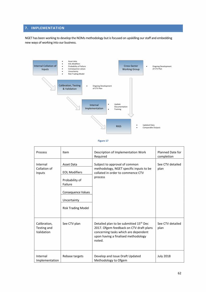
62

7. IMPLEMENTATION

NGET has been working to develop the NOMs methodology but is focused on upskilling our staff and embedding

new ways of working into our business.

Internal Collation of Inputs

Cross-Sector Working Group

Internal Implementation

RIGS

Calibration, Testing & Validation

• Asset data• EOL Modifiers• Probability of Failure• Consequence values• Uncertainty• Risk Trading Model

• Ongoing Development of CTV Plan

• Updated Data• Comparable Outputs

• Update Documentation

• Training

• Ongoing Development of CTV Plan

Figure 17

Process Item Description of Implementation Work Required

Planned Date for completion

Internal Collation of Inputs

Asset Data Subject to approval of common methodology, NGET specific inputs to be collated in order to commence CTV process

See CTV detailed plan

EOL Modifiers

Probability of Failure

Consequence Values

Uncertainty

Risk Trading Model

Calibration, Testing and Validation

See CTV plan Detailed plan to be submitted 15th Dec 2017. Ofgem feedback on CTV draft plans concerning tasks which are dependent upon having a finalised methodology noted.

See CTV detailed plan

Internal Implementation

Rebase targets Develop and Issue Draft Updated Methodology to Ofgem

July 2018

63

Methodology Final Submission August 2018

Rebased Final Targets – Ofgem Submission

September 2018

Update process documentation

Technical documentation written in draft form for submission to Ofgem subject to successful CTV.

April 2018

Subject to approval, roll out of technical documentation to business via internal governance process

April 2019

Implement Training Operational Staff Training, Planners Training

Complete

Develop monetised risk game and roll out to operational staff, planning and asset management functions

Complete

Use of a Risk Score in planning training Complete

Further training on monetised risk for asset replacement process

April 2019

RIGS Comparable Outputs

Rebase targets comparison with old targets completed

September 2018

Develop RIGS for reporting monetised risk April 2019

Run monetise risk model in parallel with Replacement Priority risk model and report both outputs in RRP

July 2019

Continuous Improvement

Continue to review inputs as part of asset management processes

ongoing

Cross Sector Working Group

Implementation of incentive mechanism

Review with Scottish TOs and Ofgem

Principles for under/over delivery

Review with Scottish TOs and Ofgem

HILP events Review with Scottish TOs and Ofgem

Table 16

64

8. ASSET SPECIFIC DETAIL

8.1. LEAD ASSETS

The following sections provide background and high level deterioration mechanisms for the lead assets.

8.1.1. CIRCUIT BREAKERS

8.1.1.1. BACKGROUND

Circuit breakers are different to other lead assets as they generally have limited condition information on an

individual asset basis. To gather additional condition information on sub components which has the potential to

affect the end of life (EoL) modifier, would require invasive work to assess the actual condition of a particular

sub component. It is undesirable to do so in the majority of situations as it would require a system outage.

Technically effective or cost justified diagnostic techniques, including continuous monitoring, are limited for use

on large populations and are not applicable for deterioration modes determining the end of life of most types

of existing circuit breaker. In addition, the deterioration age range is related to the equipment’s environment,

electrical and mechanical duty, maintenance regime and application.

In this methodology a family specific deterioration component to the EoL modifier formula is introduced to

account for missing condition information. Assignment to particular family groupings is through identification

of similar life limiting factors. Family groupings are broadly split into interrupter mechanism types.

Known deterioration modes have been determined by carrying out analysis of materials and components during

replacement, refurbishment, maintenance and failure investigation activities or following failures. The output

of the analysis reports has been used to both inform and update the relevant deterioration models. Anticipated

technical asset lives are based on the accumulated engineering knowledge of NGET’s defect and failure statistics

and manufacturer information. The method for mapping this knowledge to the end of life curve was presented

in the functional modes and effects analysis section.

8.1.1.2. DETERIORATION

Circuit breakers are made up of a number of sub-components. These sub-components deteriorate at different

rates, are different in relation to their criticality to the circuit breaker function and finally have different options

regarding intervention

Although there is a correlation between age and condition, it has been observed that there is a very wide range

of deterioration rates for individual units. The effect of this is to increase the range of circuit breaker condition

with age, some circuit breakers becoming unreliable before the anticipated life and some showing very little

deterioration well after that time.

8.1.1.3. AIR-BLAST CIRCUIT BREAKER TECHNOLOGY

As Air-Blast Circuit Breaker (ABCB) families approach their end of life an assessment is made regarding the

relative economic impact of replacement or refurbishment taking into account factors such as technological

complexity, population size and ongoing asset management capability for the design. Since most ABCB families

are no longer supported by their original equipment manufacturer, the cost and feasibility of providing parts,

skilled labour and ongoing technical support must be factored into the total cost of refurbishment. For this

65

reason, refurbishment may only be cost-effective for certain, large family types. For small families, the cost of

establishing a refurbishment programme and maintaining appropriate knowledge and support will most often

favour replacement.

Using the above approach, refurbishment has, in selected cases, proven to be an effective way to extend the

Anticipated Asset Life (AAL) for Conventional Air-Blast (CAB) and Pressurised head Air Blast (PAB) circuit

breakers.

The replacement of ABCBs is considered alongside the remaining lifetime of the associated site air system. If

removal of the last ABCBs at a site allows the site air system to be decommissioned, early switchgear

replacement may be cost beneficial when weighed against further expenditure for air system replacement

and/or on-going maintenance.

8.1.1.4. OIL CIRCUIT BREAKER TECHNOLOGY

The life-limiting factor of principal concern is moisture ingress and the subsequent risk of destructive failure

associated with the BL-type barrier bushing in bulk Oil Circuit Breakers (OCBs). A suitable replacement bushing

has been developed that can be exchanged when moisture levels reach defined criteria, but at a high cost to the

extent that is not economical to replace many bushings using this technology. Risk management of bushings has

been achieved by routine oil sampling during maintenance, subsequent oil analysis and replacement of bushings

where required. On this basis the AAL for this technology has been extended and detailed plans for replacement

or refurbishment remain to be developed.

8.1.1.5. SF6 GAS CIRCUIT BREAKER TECHNOLOGY

The bulk of the Gas Circuit Breaker population (GCB) is relatively young compared to its AAL, and therefore many

have not required replacement. A similar process to that followed for the ABCB families is being undertaken to

identify refurbishment (i.e. life extension) opportunities. Where this is not technically-feasible or cost-effective,

replacement is planned.

The GCB population includes a large number of small families, with variants and differing operating regimes, and

so the identification of large-scale refurbishment strategies may not be cost-effective. Technical and economic

evaluation as well as further development of refurbishment strategies will take place.

A significant number of SF6 circuit-breakers which are installed on shunt reactive compensation are subject to

very high numbers of operations (typically several hundred per year). The “end of life” of these circuit-breakers

is likely to be defined by number of operations (“wear out”) rather than age-related deterioration. To assist with

asset replacement planning, these circuit-breakers have been assigned a reduced asset life in this document

based on a prediction of their operating regime. Different asset lives have been assigned depending on the

circuit breaker mechanism type and/or if the circuit breaker has been reconditioned; in each case the asset life

is based on an operating duty of 300 operations per year. It is currently proposed to recondition most types of

high duty reactive switching circuit breaker when they have reached their anticipated asset life based on the

number of operations they have performed. A more detailed asset specific strategy for replacement or

refurbishment of these categories of circuit-breakers is being developed in terms of the actual number of

operations and their forecast operating regime.

66

8.1.2. TRANSFORMERS AND REACTORS

8.1.2.1. BACKGROUND

Transformers and reactors share similar end of life mechanisms since they are both based on similar

technologies. The same scoring method is therefore applied to calculate the EoL modifier. For simplicity within

this section the term transformer is used to mean both transformer and reactor.

Transformers are assigned an EoL modifier according to the condition inferred from diagnostic results, the

service history, and post mortem analysis of other similar transformers.

The health of the overall transformer population is monitored to ensure that replacement/refurbishment

volumes are sufficient to maintain sustainable levels of reliability performance, to manage site operational issues

associated with safety risks and to maintain or improve environmental performance in terms of oil leakage.

The process by which transformers are assigned an EoL modifier relies firstly on service history and failure rates

specific to particular designs of transformers and secondly on routine test results such as those obtained from

Dissolved Gas Analysis (DGA) of oil samples. When either of these considerations gives rise to concern, then

where practicable, special condition assessment tests (which usually require an outage) are performed to

determine the appropriate EoL modifier. Special condition assessment may include the fitting of a continuous

monitoring system and the analysis of the data to determine the nature of the fault and the deterioration rate.

The elements to be taken into account when assigning an EoL modifier are:

1. Results of routine condition testing

2. Results of special condition assessment tests

3. Service experience of transformers of the same design, and detailed examination of decommissioned

transformers

4. Results of continuous monitoring where available

The following additional condition indications shall be taken into account when deciding the

repair/replacement/refurbishment strategy for a particular transformer:

1. Condition of oil

2. Condition of bushings

3. Condition of coolers

4. Rate of oil loss due to leaks

5. Condition of other ancillary parts and control equipment

6. Availability of spare parts particularly for tap-changers

8.1.2.2. TRANSFORMER AND REACTOR DETERIORATION

Thermal ageing of paper is the principal life limiting mechanism for transformers which will increase the failure

rate with age. This failure mechanism is heavily dependent on design and evidence from scrapped transformers

indicates a very wide range of deterioration rates. Knowledge of the thermal ageing mechanism, other ageing

mechanisms and the wide range of deterioration rates are used to define the anticipated asset lives for

transformers.

In addition to the above fundamental limit on transformer service life, experience has shown that a number of

transformer design groups have inherent design weaknesses which reduce useful service life

67

The condition of transformers can be monitored through routine analysis of dissolved gases in oil, moisture and

furfural content together with routine maintenance checks. Where individual test results, trends in test results

or family history give cause for concern, specialist diagnostics are scheduled as part of a detailed condition

assessment. Where appropriate, continuous monitoring will also be used to determine or manage the condition

of the transformer.

Methods exist to condition assess transformers and indicate deterioration before failure, however the time

between the first indications of deterioration and the transformer reaching a state requiring replacement is

varied and can depend on factors such as the failure mechanism, the accuracy of the detection method, and the

relationship between system stress and failure. For this reason the transformer models periodically require

updating (supported by evidence from post-mortem analysis) as further understanding of deterioration

mechanisms is acquired during the transformer life cycle.

8.1.2.3. INSULATING PAPER AGEING

The thermal ageing of paper insulation is the primary life-limiting process affecting transformers and reactors.

The paper becomes brittle, and susceptible to mechanical failure from any kind of shock or disturbance.

Ultimately the paper will also carbonise and cause turn to turn failure, both mechanisms leading to dielectric

failure of the transformer. The rate of ageing is mainly dependent upon the temperature and moisture content

of the insulation. Ageing rates can be increased significantly if the insulating oil is allowed to deteriorate to the

point where it becomes acidic.

The thermal ageing of paper insulation is a chemical process that liberates water. Any atmospheric moisture

that enters the transformer during its operation and maintenance will also tend to become trapped in the paper

insulation. Increased moisture levels may cause dielectric failures directly or indirectly due to formation of gas

bubbles during overload conditions.

The paper and pressboard used in the construction of the transformer may shrink with age which can lead to

the windings becoming slack. This compromises the ability of the transformer windings to withstand the

electromagnetic forces generated by through-fault currents. Transformer mechanical strength may be

compromised if it has experienced a number of high current through faults during its lifetime and the internal

supporting structure has been damaged or become loose.

End of life as a result of thermal ageing will normally be supported by evidence from one or more of the following

categories:

1. Post-mortem (scrapping) evidence (including degree of polymerisation test results) from units of similar

design and load history

2. High and rising furfural levels in the oil

3. High moisture content within the paper insulation

4. Evidence of slack or displaced windings (frequency response tests or dissolved gas results)

8.1.2.4. CORE INSULATION

Deterioration of core bolt and core-to-frame insulation can result in undesirable induced currents flowing in the

core bolts and core steel under certain load conditions. This results in localised overheating and risk of Buchholz

alarm/trip or transformer failure as free gas is generated from the localised fault. It is not normally possible to

repair this type of fault without returning the transformer to the factory. Evidence of this end of life condition

would normally be supported by DGA results together with evidence from decommissioned transformers of

similar design. Insertion of a resistor into the core earth circuit can reduce or eliminate the induced current for

a period of time.

68

8.1.2.5. THERMAL FAULT

Transformers can develop localised over-heating faults associated with the main winding as a result of poor

joints within winding conductors, poor oil-flow or degradation of the insulation system resulting in restrictions

to oil flow. This is potentially a very severe fault condition. There is not normally a repair for this type of fault

other than returning the transformer to the factory. Evidence of this end of life condition would normally be

supported by dissolved gas results together with forensic evidence from decommissioned transformers of

similar design.

8.1.2.6. WINDING MOVEMENT

Transformer windings may move as a result of vibration associated with normal operation or, more commonly,

as a result of the extreme forces within the winding during through fault conditions. The likelihood of winding

movement is increased with aged insulation as outlined above. Where evidence of winding movement exists,

the ability of the transformer to resist subsequent through faults is questionable and therefore the unit must be

assumed not to have the strength and capability to withstand design duty and replacement is warranted. There

is no on-site repair option available for this condition. Winding movement can be detected using frequency

response test techniques and susceptibility to winding movement is determined through failure evidence and

evidence of slack windings through dissolved gas results.

8.1.2.7. DIELECTRIC FAULT

In some circumstances transformers develop dielectric faults, where the insulation degrades giving concern over

the ability of the transformer to withstand normal operating voltages or transient overvoltage. Where an

internal dielectric fault is considered to affect the main winding insulation, irreparable damage is likely to ensue.

This type of condition can be expected to worsen with time. High moisture levels may heighten the risk of

failure. Evidence of a dielectric problem will generally be based on operational history and post-mortem

investigations from units of similar design, supported by DGA. Various techniques are available to assist with

the location of such faults, including partial discharge location techniques. If evidence of an existing insulation

fault exists and location techniques cannot determine that it is benign, then the transformer should be

considered to be at risk of failure.

8.1.2.8. CORROSIVE OIL

In certain cases high operating temperatures combined with oil containing corrosive compounds can lead to

deposition of copper sulphide in the paper insulation, which can in turn lead to dielectric failure. This

phenomenon may be controlled by the addition of metal passivator to the oil, however experience with this

technique is limited and so a cautious approach to oil passivation has been adopted. Regeneration or

replacement of the transformer oil may be considered for critical transformers or where passivator content is

consumed quickly due to higher operating temperatures.

8.1.3. UNDERGROUND CABLES

8.1.3.1. BACKGROUND

Cable system replacements are programmed so that elements of the cable systems are replaced when the

safety, operational or environmental risks of continued operation meet defined criteria.

69

Replacement of cable systems are based on a number of metrics including age. These metrics only include a

few condition-related components since there is limited information that can be obtained on how deteriorated

a cable actually is. Further condition information could be obtained by digging up and taking samples of a cable,

but this is not practical, would be costly and could also cause further failures. Metrics such as the cost of repairs

are taken into account when determining if a cable has reached the end of its life. While this is not the most

desirable metric from an analytical perspective, it does reflect historical practice and is justifiable from a

consumer value perspective.

The factors to be taken into account when determining an EoL modifier are:

1. Historical environmental performance

2. Historical unreliability

3. Risk of tape corrosion or sheath failure

4. Results of condition assessment and other forensic evidence

5. Service experience of cable systems of similar design

6. Number of defect repairs

7. Number of cable faults

8. Duty in terms of how much time annually a cable is running at or above its designed rating

9. Bespoke nature and issues associated with specific cable systems


End of technical life will generally be due to the deterioration of the main cable system; this may be associated

with either mechanical or electrical integrity or withstand capability.

With the exception of cables vulnerable to reinforcing tape corrosion and cables where a known manufacturing

defect has occurred (e.g. lead sheath deterioration), cable systems have generally given reliable operation and

there is limited experience of long term deterioration mechanisms.

Cables can be split broadly into two classes for the purposes of understanding the end of life of this asset class,

these are fluid filled cables and solid dielectric cables. In general the cable circuit will only meet the criteria for

replacement where refurbishment as described above will not address condition and performance issues and

guarantee compliance with statutory requirements.

8.1.3.3. END OF LIFE MECHANISMS AFFECTING BOTH TYPES OF CABLES

8.1.3.3.1. LEAD AND ALUMINIUM SHEATH DETERIORATION

Fatigue and intercrystalline cracking, and defects introduced during manufacture can cause oil leaks to develop.

It is not generally possible to predict when a given cable section will fail as a result of this failure mode. Local

repairs are not generally effective as sheath deterioration is usually distributed along the cable. End-of-life is

reached where sheath deterioration is resulting in significant and widespread oil-loss (relative to duties in

respect of recognised code of practice) along the cable length.

8.1.3.3.2. BONDING SYSTEM

Water ingress to link boxes causes deterioration of cross-bonding systems and leaves the link box and its Sheath

Voltage Limiters (SVLs) vulnerable to explosive failure under fault conditions. Specific evidence shall be gathered

through condition assessment to support end-of-life determination. This issue will in general be addressed by

replacement of specific components during circuit refurbishment activity or enhanced routine maintenance.

70

8.1.3.3.3. COOLING SYSTEM

The life of a cable’s cooling system is much shorter than the lifetime of the overall cable asset. Therefore mid-

life intervention maybe required to replace the cable cooling system components. While this is not the end of

the life of the cable it is an important consideration as the cable is not able to do what it was designed to do

with a failed cooling system. Cooling systems tend to be unique to each cable route. Loss of the cooling capacity

can typically reduce circuit rating by 40%. Most problems are experienced with the original control systems

which are now obsolete. Aluminium cooling pipes are vulnerable to corrosion and plastic pipes are vulnerable

to splitting, which can result in water leaks. Cooling control system and pumping equipment will also require

replacement prior to the main cable system in line with circuit specific assessment. In general cooling pipework

should be managed through maintenance to achieve the asset life of the main cable system.

8.1.3.4. FLUID FILLED CABLE END OF LIFE MECHANISMS

8.1.3.4.1. REINFORCING TAPE CORROSION

Reinforcing tapes are used to retain the oil pressure for cables with lead sheaths. Corrosion of the tapes in

certain early BICC cables and AEI cables results in the tapes breaking, the sheath splitting and consequential oil

leaks. Methods are being developed for predicting failure using corrosion rates determined through sampling

in combination with known operating pressures, and also using degradation mechanism models. Local repairs

are not considered effective mitigation as corrosion is usually distributed along the cable. End-of-life of the

cable system is in advance of widespread predicted tape failure. The lead times for cable replacement schemes

are considerably greater than the time to deteriorate from broadly acceptable to unacceptable cable system

performance for this failure mode. This implies that pre-emptive action is required to minimise the likelihood of

failure occurring. Acceptable performance is where the cable can be repaired on an ad-hoc basis; unacceptable

performance is where the corrosion is distributed along a significant number of sections of the route.

8.1.3.4.2. STOP JOINT DETERIORATION

Stop-joint failure presents significant safety, reliability and environmental risk. End-of-life for stop joints will be

justified based upon oil-analysis data or forensic evidence from similar designs removed from service. Stop joint

deterioration can be addressed via refurbishment and would not alone drive replacement of the cable system.

8.1.3.4.3. CABLE JOINT DETERIORATION

In general cable joint deterioration can be addressed via refurbishment and would not alone drive replacement

of the joint or cable system.

8.1.3.4.4. OIL-ANCILLARIES

Corrosion of oil tanks, pipework and connections, and pressure gauges can result in oil leaks and incorrect

operation of the ancillaries. Specific evidence shall be gathered through condition assessment to support end-

of-life determination. This issue will in general be addressed by replacement of specific components during

circuit refurbishment activity or enhanced routine maintenance.

71

8.1.3.4.5. ENVIRONMENTAL CONSIDERATIONS

NGET has a statutory obligation to comply with the Water Resources Act 1991/Water Resources (Scotland) Act

2013 and to fulfil its commitments with respect to its Environmental Statement. Utilities demonstrate

compliance with the requirement of the Act through adherence to the guidance provided.

A factor to consider in determining anticipated asset life is when it is no longer reasonably practicable to comply

with the requirements of the above legislation and guidance, and maintain a sustainable level of circuit

availability.

8.1.3.4.6. SOLID XLPE FILLED CABLE END OF LIFE MECHANISMS:

Transmission circuits have been installed at at 132kV and 275kV since 1988 in the UK. Limited examples at lower

voltages in substations exist back to 1968. There is limited service experience at 400kV. Provided high standards

of manufacture and installation are available, the risk of early-life failures will be avoided. The existing asset

lifetime estimates are largely based on the tests conducted at type registration, e.g. the time to fault when

tested at voltages very much greater than that intended for operational use. Statistics were then used to justify

the probability a cable would reach a specific age. End of life mechanisms have not been encountered in the UK

at this time. The long-term deterioration mechanisms would benefit from further research and development.

Possible failure modes6 that XLPE cables may exhibit are:

• Insulation deterioration due to natural ageing due to thermal cycling, mechanical aggression and

defects.

• Polyethylene oversheaths have known risks of photo- and thermal-degradation into lactones, esters,

ketones and carboxylic acid.

• Water treeing, arising from partial discharge in a cable. This failure mode arises mostly as a result of

moisture ingress; which itself can arise from outer sheath damage, poor or non-existent water barriers

or outer metallic sheath corrosion. It should be noted that moisture can penetrate even an intact

oversheath; albeit Polyethlyene is a much better barrier than PVC as used on older cable technologies.

The figure below illustrates this failure mode.

• Electric treeing due to a defect in the insulation, partial discharge or thermal ageing. Such a defect

could also occur at cable joints; as the risk of contamination is considerably higher for such an assembly

in the field rather than the clean-room conditions of the production line.

• Arcing from phase conductor to the outer sheath. Such a fault is unlikely without external influences,

such as excessive mechanical force on the cable sheath, or deformation of the conductor and insulation.

• Thermal runaway, in the event that the material surrounding the cable does not posess the thermal

conductivity and heat capacity appropriate to the losses encountered on the cable. Thermal runaway

is possible as a result of third party influences; for example where burial depths are unintentionally

increased without notification.

National Grid does not at this time have experience of all these failure modes. Circuit loadings inherent to design

of the system to the SQSS in routine operation, are relatively low. The populations are also relatively young; the

oldest example at transmission voltage in the UK dates from 1988. The failure modes listed are highly

interlinked, for example the condition and quality of the cable installation have bearing on the risk of water

treeing and arcing. The deterioration of the insulation appears mostly to be associated with the age of the cable,

though operational duty and installation environment also appear to have bearing on condition. Evaluation of

6 EA Technology - Reducing Failure Rates and Better Management of Underground Cable Networks

72

condition is, as noted above, problematic without destructive testing, there is therefore a strong desire to devise

and deploy alternative means of evaluating condition rather than relying on age as an indicator alone.

8.1.4. OVERHEAD LINES

8.1.4.1. GENERAL APPROACH

Routes are fully refurbished, or have critical components replaced, to maintain reliability (including a level of

resilience to extreme weather conditions), operational risk and safety performance. In addition, conductors

should retain sufficient residual mechanical strength to facilitate safe replacement by tension stringing methods

at end of life.

Technical asset lives for OHL components in various environments have been predicted using historical condition

information from previous OHL replacement schemes, condition samples taken on existing assets, and an

understanding of deterioration mechanisms.

Scoring assessments are made on sections of circuit that are typically homogenous in conductor type, installation

date and environment.


8.1.4.1.1. CONDUCTORS

Conductor end of life condition is a state where the conductor no longer has the mechanical strength (both

tensile and ductility) required to support the combination of induced static and environmental loads.

Two main deterioration mechanisms exist:

1. Corrosion, primary cause pollution either saline or industrial

2. Wind induced fatigue, common types

a. Aeolian vibration (low amplitude high frequency oscillation 5 to 150 Hz)

b. sub-conductor oscillation (bundles conductors only) produced by forces from the shielding

effect of windward sub-conductors on their leeward counterparts

c. galloping (high-amplitude, low-frequency oscillation)

d. wind sway

Conductor fatigue is usually found at clamp positions where the clamp allows more interstrand motion within

the conductor, leading to fretting of the internal layers. Loss of strand cross-section follows, then fatigue

cracking, and finally strand breakage. This form of degradation is generally the life-limiting factor for quad

bundles, clamping positions on twin bundles can also be affected

Conductor corrosion is also usually found at clamp positions. Interwoven conductor strands open up at these

points allowing for easier ingress of corroding chlorides, sulphates and moisture etc. The zinc galvanising of the

core wires is corroded, eventually exposing the underlying steel. A galvanic corrosion cell is then created where

the aluminium wire is sacrificial. The loss of cross section of aluminium leads to greater heat transfer to the steel

core increasing the risk of core failure. Additionally, some spacer clamps with elastomer bushings that contain

carbon and have a low resistance also lead to galvanic corrosion of aluminium strands, reducing thickness,

strength and ductility.

In addition end of life may be advanced, in rare instances, due to an unexpected load or events such as extreme

wind ice or heat which overlead (stress) the conductor beyond its design capability. Quality of the original

73

manufacturing could also be an issue (galvanising defects) but there is not much evidence for this in conductor

condition assessment data.

8.1.4.1.2. INSULATORS

The end of life occurs when the increased risk of flashover (loss of dielectric strength) reaches an unacceptable

level due to condition, which may or may not result in mechanical failure of the string, or a decrease in

mechanical strength due to corrosion of the steel pin.

8.1.4.1.3. FITTINGS - SPACERS, SPACER DAMPERS AND VIBRATION DAMPERS

The functional end of life of spacers, spacer dampers and vibration dampers occurs at the point at which the

conductor system is no longer protected, and conductor damage starts to occur.

These items are utilised to protect the conductor system from damage. The main deterioration mechanism is

wear or fatigue induced through conductor motion. Corrosion in polluted environments can also be an issue

particularly inside clamps

Wear damage to trunnions and straps of suspension clamps occurs due to conductor movement. The wear has

been greatest in areas of constant wind, i.e. higher ground, flat open land and near coasts. For quad lines, in

particular at wind exposed sites, wear can be extensive and rapid failures of straps, links, shackles and ball-ended

eye links can occur. This is one of the best indicators of line sections subject to sustained levels of wind induced

oscillation and hence where future conductor damage is likely to become a problem.

Most conductor joints for ACSR have been of the compression type, although bolted joints are used in jumpers.

Overheating joints can arise from inadequate compression along the length of the joint, mainly due to either

poor design or installation problems. These allow moisture penetration and oxidation of the internal aluminium

surfaces between the joint and conductor. The resistive aluminium oxide reduces the paths for current flow and

may cause micro-arcing within the joint. The consequence of this deterioration is that the joint becomes warm

which further increases the rate of oxidation. Over a period of time, the resistive paths can result in excess

current flowing in the steel core of the conductor, which can then overheat and rupture.

8.1.4.1.4. SEMI-FLEXIBLE SPACERS

These are fitted in the span and the semi-flexibility comes from either elastomer liners, hinges or stranded steel

wire depending on the manufacturer. End of life is defined by perishing of the elastomer lining or broken/loose

spacer arms. These allow for excessive movement of the conductor within the clamp leading to severe conductor

damage in small periods of time (days to months, depending on the environmental input). The elastomer lining

of the Andre spacer type also causes corrosion of conductor aluminium wires due to its carbon content and

subsequent galvanic corrosion. A common finding of conductor samples at these positions is strands with

significantly poorer tensile and torsional test results. This is a hidden condition state unless it manifests in broken

conductor strands that are visible on inspection.

Replacement of these spacers has been necessary on routes that are heavily wind exposed at approximately 25

years. There are many examples still in service beyond their anticipated life of 40 years where visual end of life

characteristics have not yet been met. As the condition of the associated conductor within or near the clamp

can remain hidden, certain families of this type of spacer such as the ‘Andre’ are identified for the increased risk

they pose to conductor health.

74

8.1.4.1.5. SPACER DAMPERS

As the service history of spacer dampers is limited, extensive data on their long-term performance and end of

life is not yet available. The spacer arms are mounted in the spacer body and held by elastomer bushes. This

increased flexibility should provide the associated conductor system with more damping and greater resilience

to wind induced energy. End of life criteria will be defined by broken/loose spacer arms that allow for excessive

movement of the conductor/clamp interface.

8.1.4.1.6. VIBRATION DAMPERS

Stockbridge dampers have always been used for the control of Aeolian vibration, a minimum of one damper

being installed at each end of every span on each subconductor. For long spans (where specified by the

manufacture) two or more may be used. End of life is defined by loss of damping capability which is visually

assessed in the amount of ‘droop’ in and wear of the messenger cable between damper bells. The useful life of

a damper is constrained by wind energy input and corrosion of the messenger wire connection with the damper

bells. In areas of high wind exposure there is evidence that dampers have required replacement after 10 to 15

years. There are however many more examples of dampers operating beyond their anticipated life with no visual

signs of end of life.

8.2. LEAD ASSETS – PARAMETERS FOR SCORING

Examples of the methodology used for scoring against the parameters outlined below are contained within the

NGET Licensee Specific Appendices

8.2.1. CIRCUIT BREAKER PARAMETERS

8.2.1.1. SCORING PROCESS

Circuit breakers will be assigned an end of life modifier according to the formula below. The maximum of the

components as shown is determined, and it is capped at 100.

𝐸𝑂𝐿𝑚𝑜𝑑 = max (𝐴𝐺𝐸𝐹𝐴𝐶𝑇𝑂𝑅 , 𝐷𝑈𝑇𝑌𝐹𝐴𝐶𝑇𝑂𝑅 , 𝑆𝐹6𝐹𝐴𝐶𝑇𝑂𝑅 , 𝐷𝐸𝐹𝐸𝐶𝑇𝐹𝐴𝐶𝑇𝑂𝑅 , 𝐹𝐴𝑀𝐼𝐿𝑌𝐹𝐴𝐶𝑇𝑂𝑅 )

Equation 51

The EOL modifier is therefore determined based on the maximum of its constituent parts. AGE_FACTOR,

DUTY_FACTOR, SF6_FACTOR and FAMILY_FACTOR are non-dimensional variables with possible values between

0 and 100.

𝐴𝐺𝐸_𝐹𝐴𝐶𝑇𝑂𝑅 = C1 ×FSDP×Age

𝐴𝐴𝐿

Equation 52

• Age: Reporting year - Installation year (years)

• C1: a scaling factor to convert Age to a value in the range 0 to 100. The method for calculating C1 is

described at the end of this section

75

• AAL is the anticipated asset life determined through FMEA analysis. The end of life curve described in

the Failure Modes and Affects analysis section can be used to determine AAL, which is the 50% point

on the respective end of life failure mode curve. The process for deriving these failure mode curves,

which we use to determine AAL, are themselves estimated using historical data and engineering

expertise. Further explanation is available in the section of this methodology discussing FMEA.

• FSDP is a family specific deterioration correction function described below. This is a function multiplier

to convert AGE from a linear function to an exponential function. This has the effect of decreasing the

relative significance of lower values of AGE

• The AAL value is determined through interpretation of historic data associated with the type and

manufacturer of the circuit breaker. Other factors can also influence the AAL including locational

factors such as whether or not the asset is indoors or outdoors. Other locational factors such as

proximity to high corrosion potential are not included as these are covered through maintenance

activities to ensure that the asset achieves its Anticipated Life.

8.2.1.2. DUTY_FACTOR

The duty of each circuit breaker asset is determined using the following formula:

𝐷𝑈𝑇𝑌_𝐹𝐴𝐶𝑇𝑂𝑅 = C1×𝐹𝑆𝐷𝑃×max (((𝑂𝐶)

(𝑀𝑂𝐶)) , (

(𝐹𝐶)

(𝑀𝐹𝐶)))

Equation 53

Where:

• OC is the current asset operational count

• MOC is the expected max asset operational count over a lifetime. For older circuit breakers this is

determined through liaison with suppliers, and for newer circuit breakers this is determined during type

testing

• FC is the current accumulated fault current

• MFC is the max permissible fault current over a lifetime. The value for MFC is set to 80% of the value

of the maximum rated value for the asset

FC and MFC are determined through liaison with suppliers who confirm operational limits for the mechanism

and interrupter.

Note that the DUTY_FACTOR has been normalised to account for variations in the asset life of the circuit breaker

family. This normalisation means that the end of life modifier of a circuit breaker from one family can be

compared to the end of life modifier of a circuit breaker from a different family. Age and other duty related

metrics are important due to the lack of more specific condition information.

8.2.1.3. FAMILY SPECIFIC DETERIORATION PROFILE (FSDP)

The Family Specific Deterioration profile accounts for the expected deterioration of an asset. This is needed as

there is limited availability of Asset Specific condition information. This function is based on duty value D which

is given by the following formula:

76

𝐷 = max (𝑂𝐶

𝑀𝑂𝐶,𝐹𝐶

𝑀𝐹𝐶,𝐴𝐺𝐸

𝐴𝐴𝐿)

Equation 54

The family specific deterioration function is determined using the function:

𝐹𝑆𝐷𝑃 = 𝑒𝑘∗𝐷2− 1

Equation 55

This parameter k is determined such that when D=1.0 then FSDP=1.0. This gives a value of k=0.694. FSDP is

capped at 1.0.

This function ensures that the impact of family specific deterioration is correctly considered in the health score

formula.

Figure 18

The curve will generate a value from 0 to 1 depending on the duty of the asset. This curve is used within this

method due to the lack of condition information, and allows us to accelerate or suppress duty values depending

on the deterioration we would expect for that asset family. Note that while the shape of the curve is fixed, the

duty value (D) captures family specific factors such as anticipated asset life, maximum fault current and

maximum number of operations.

8.2.1.4. SF6_FACTOR (SF6)

The SF6_FACTOR calculation maps the reported leakage of a circuit breaker to a score of between either 0 or

100. A score of 100 is assigned where major leakage is deemed to have occurred. Leaking time is the time in

years that the asset has had a non-zero Leakmass, Leakrate, or Leakcombined.

𝑆𝐹6𝐹𝐴𝐶𝑇𝑂𝑅 = 𝑀𝑎𝑥(𝐿𝑒𝑎𝑘𝑀𝑎𝑠𝑠 , 𝐿𝑒𝑎𝑘𝑅𝑎𝑡𝑒 , 𝐿𝑒𝑎𝑘𝐶𝑜𝑚𝑏𝑖𝑛𝑒𝑑 ) + 𝐿𝑒𝑎𝑘 𝐷𝑢𝑟𝑎𝑡𝑖𝑜𝑛 ∗ 𝐿𝑒𝑎𝑘𝑖𝑛𝑔𝑡𝑖𝑚𝑒

Equation 56

Leakmass is a score dependent on the mass of SF6 leakage (kg) within the previous financial year.

0

0.1

0.2

0.3

0.4

0.5

0.6

0.7

0.8

0.9

1

0 0.2 0.4 0.6 0.8 1 1.2

FSD

P -

Co

rre

ctio

n v

alu

e

D

77

Mass of Leakage (kg) Significance Leakmass Score

<10kg Insignificant 0

>=10kg Significant 60

>=50kg Major Leakage 75

Table 17

Leakrate a score dependent on proportion of total installed mass of SF6 that has leaked within the previous

financial year

𝐿𝑒𝑎𝑘𝑎𝑔𝑒 𝑟𝑎𝑡𝑒 =𝐿𝑒𝑎𝑘𝑀𝑎𝑠𝑠

𝐴𝑠𝑠𝑒𝑡 𝑆𝐹6 𝐼𝑛𝑣𝑒𝑛𝑡𝑜𝑟𝑦

Equation 57

where Asset SF6 Inventory is the Reported volume of SF6.

Mass of Leakage (kg) Significance Leakrate Score

<5% Insignificant 0

>=5% Signifcant 60

>=10% Major Leakage 75

Table 18

Leakcombined=100 if both the mass of leakage is >=50kg and leakage rate is >=10%, otherwise Leakcombined=0

Leakduration ensures that a leaking asset for the last two or five (dependant on current severity of leak) years will

be assigned a score of 100.

Leakage Duration Leakduration Score

First year of leak 0

Leak mass score=60 8

Leak mass score=75 12.5

Table 19

Any asset classified with EOL modifier of 60 or 75 due to SF6 leakage will undergo a significant intervention

within a 5 year or 2 year timeframe respectively. It is expected that an asset classified with a health score of 75

today will reach a health score of 100 within 2 years, which has been set-up to reflect legislation that significant

SF6 leakers should be repaired within 2 years. The decision over which type of intervention to carry out, whether

that is repair, reconditioning, refurbishment or replacement, will be cost justified for the expected benefit to the

consumer. This means that risk will be reduced through the most cost justified intervention, which may not

necessarily be asset replacement.

Whilst there are pre-existing technologies that exist to carry out minor repairs to stop SF6 leaks, analysis of these

repairs demonstrates that in the majority of instances they are temporary in nature and a further major

intervention is then required to permanently repair the asset.

Broadly there are two functional requirements for a Gas Circuit Breaker. Firstly it must be able to break load,

and secondly it must be able to retain the Insulating Medium. This is based on the requirements described in

the Fluorinated Greenhouse Gases Regulations 2015, which places significant limits on permitted Leakage.

1. Operators of equipment that contains fluorinated greenhouse gases shall take precautions to prevent

the unintentional release (‘leakage’) of those gases. They shall take all measures which are technically

and economically feasible to minimise leakage of fluorinated greenhouse gases.

78

2. Where a leakage of fluorinated greenhouse gases is detected, the operators shall ensure that the

equipment is repaired without undue delay. (Chapter 2 Article 3 Sections 2 and 3 from http://eur-

lex.europa.eu/legal-content/EN/TXT/PDF/?uri=CELEX:32014R0517&from=EN)

8.2.1.5. DEFECT_FACTOR

This factor is currently set to zero awaiting improved classification in data collection process

8.2.1.6. FAMILY FACTOR

Circuit breaker families that are exhibiting life limiting factors, which do not align to the other factors in the

formulation, needs to be captured by the end of life modifier scoring process. As such a factor will be applied

to drive intervention due to end of life to be approximately within a specific timeframe.

Asset family modifier Score

Intervention within 2 years 80



Table 20

8.2.1.7. PROCEDURE FOR DETERMINING C1

This value of this parameter is determined by calculating a value for EOL modifier from historical switchgear

data. The C1 value is tuned so that a reasonable translation between historical AHI’s, which were calculated

under the previous RIIO-T1 volume based methodology, and EOL modifier is achieved. Assets that were classed

as AHI1 previously should normally have a score of 100 under the new methodology. This approach is consistent

with the theme of the direction, as it enables a translation from previously classified AHI’s.

Based on this approach the parameter is fixed as 𝐶1 = 5/6.

8.2.1.8. EOL MODIFIER CALCULATION EXAMPLE

The following table shows three assets with example data that will allow us to determine the EOL modifier

Component Example Asset 1 Example Asset 2 Example Asset 3

Asset Operation Count (OC) 350 3000 350

Max Asset Operation Count (MOC) 5000 5000 5000

Accumulated Fault Current (FC) 400 400 1000

Max Permissible Fault Current (MFC) 1400 1400 1400

Anticipated Asset Life (AAL) 45 45 45

SF6 leakage (kg) 2 10 1

Age 40 20 15

Table 21

Applying the relevant formula presented in the above sections yields the following output.

http://eur-lex.europa.eu/legal-content/EN/TXT/PDF/?uri=CELEX:32014R0517&from=EN

http://eur-lex.europa.eu/legal-content/EN/TXT/PDF/?uri=CELEX:32014R0517&from=EN

79

Example Asset 1 Example Asset 2 Example Asset 3

D (in FSDP) 0.89 0.6 0.71

FSDP 0.72 0.28 0.41

AGE_FACTOR 53.19 10.23 11.23

DUTY_FACTOR 16.73 13.94 24.16

SF6_FACTOR 0 60 0

EOL Modifier 53.2 60 24.2

Table 22

The EOL Modifier in example asset 1 is driven by age factor, example 2 is driven by SF6 factor and example 3 is

driven by the duty factor (in particular the accumulated fault current).

The EOL modifier calculation proposed here facilitates a reasonable translation from the AHI’s utilised within

the existing RIIO-T1 methodology. An initial validation has been performed to calculate EOL modifier over a

range of assets and then comparing to the AHI determined under the existing methodology.

It should be noted that placing a cap on the age related components of health score would substantially impair

the translation from the previous AHI to health score.

8.2.2. TRANSFORMER AND REACTOR PARAMETERS


The scoring process needs to takes account of the four failure modes – dielectric, mechanical and thermal as

well as issues with other components that may significantly impact the remaining service life. The end of life

modifier is determined according to the following formula:

𝐸𝑂𝐿𝑚𝑜𝑑 = (1 − (1 −𝐷𝐶𝐹

100) (1 −

𝑇𝐶𝐹

100) (1 −

𝑀𝐶𝐹

100) (1 −

𝑂𝐶𝐹

100)) ∗ 100

Equation 58

The components of the end of life modifier are assigned using the scoring system described below. The

component OCF (other component factor) is a factor that accounts for other issues that can affect transformer

end of life. The maximum value of EOLmod is 100.

As far as possible National Grid uses actual condition indicators rather than extrapolating condition from load

and temperature over time. This approach is more feasible with large transformers and is less dependent on the

availability of historical data. The approaches are not mutually exclusive and loading data is important to the

correct interpretation of some condition indicators such as oil test results

8.2.2.2. DIELECTRIC CONDITION FACTOR (DCF)

Dielectric condition is assessed using dissolved gas analysis (DGA) results. The score can be increased if the

indication is that the individual transformer is following a trend to failure already seen in other members of the

family. Where it is known that the indications of partial discharge are coming from a fault that will not ultimately

lead to failure e.g. a loose magnetic shield then the score may be moderated to reflect this but the possibility of

this masking other faults also needs to be taken into account.

80

Score Dielectric Condition Criteria

0 All test results normal: no trace of acetylene; normal levels of other gases and no indication of

problems from electrical tests.

2 Small trace of acetylene in main tank DGA or stray gassing as an artefact of oil type,

processing or additives. Not thought to be an indication of a problem.

10 Dormant, intermittent or low level arcing/sparking or partial discharge fault in main tank.

30 Steady arcing/sparking or partial discharge fault in main tank.

60 Indications that arcing/sparking fault is getting worse.

100 Severe arcing/sparking or partial discharge fault in main tank – likely to lead to imminent

failure.

Table 23

8.2.2.3. THERMAL CONDITION FACTOR (TCF)

Thermal condition is assessed using trends in DGA and levels of furans in oil. Individual Furfural concentration

(FFA) results are unreliable because they can be influenced by temperature, contamination, moisture content

and oil top ups, therefore a trend needs to be established over a period of time. The presence of 2 Furfural

(2FAL) is usually required to validate the FFA result and the presence or absence of methanol is now being used

to validate (or otherwise) conclusions on thermal score. Thermal condition is understood to include ageing and

older, more heavily used and/or poorly cooled transformers tend to have higher scores. The score can be

increased if the indication is that the individual transformer is following a trend to failure already seen in other

members of the family.

Score Thermal Condition Criteria

0

No signs of paper ageing including no credible furans >0.10ppm and methanol ≤0.05ppm.

The credibility of furan results usually depends on the presence of 2 Furfural (2FAL).

2

Diagnostic markers exist that could indicate paper ageing (including credible furans in the

range 0.10-0.50ppm) or are thought to be the result of contamination.

The credibility of furan results usually depends on the presence of 2 Furfural (2FAL).

10

Indications or expectations that the transformer is reaching or has reached mid-life for example: credible furans in the range 0.51-1.00ppm or stable furans >1ppm possibly as a result of historic paper ageing.

and/or

DGA consistent with low temperature overheating e.g. raised levels of methane or ethane in the main tank.

81

and/or

Transformers with diagnostic markers resulting from oil contamination (e.g. furans, specifically 2FAL) that may mask signs of paper ageing.

30

Moderate paper ageing for example: credible furans consistently > 1ppm with a clear upward trend.

and/or

Significant overheating fault e.g. steadily rising trend of ethylene in main tank DGA.

60

Advanced paper ageing for example: credible furans > 1.5ppm showing a clear upward trend (even if the furan level has subsequently stabilised) or following the indications of a sister unit found to be severely aged when scrapped.

and/or

Significant and worsening overheating fault.

100

Very advanced paper ageing for example: credible furans >2ppm with an upward trend or following the indications of a sister unit found to be severely aged when scrapped.

and/or

Serious overheating fault.

Table 24

Electrical test data may be used to support a higher thermal score where they show poor insulation condition.

Electrical tests can provide further evidence to support the asset management plan for individual transformers

e.g. where a significant number of oil tops ups have been required for a particularly leaky transformer and it is

suspected that this is diluting the detectable Furans in the oil. However experience shows that not all poor

thermal conditions can be detected by electrical tests which is why DGA data remains the focus for scoring the

Thermal Condition Factor.

While age and AAL are not explicitly considered as part of the transformer EOL modifier scoring process, the

thermal condition score is a fairly good indicator of the age of an asset. The DGA results obtained from oil

samples will generally show signs indicating the aging of a transformer including increased levels of furans.

8.2.2.4. MECHANICAL CONDITION FACTOR (MCF)

Mechanical condition is assessed using Frequency Response Analysis (FRA) results.

Score Mechanical Condition Criteria

0 No known problems following testing.

1 No information available.

3

Anomalous FRA results at last measurement which are suspected to be a measurement problem and not an indication of mechanical damage.

and/or

Corrected loose clamping which may reoccur.

10

Loose clamping

or

Following the indications of a sister unit found to have had compromised mechanical integrity/short circuit strength

82

or

A design known to have a poor short circuit design.

30 Suspected mechanical damage to windings. This does not include cases where the damage is confirmed.

60 Loose or damaged clamping likely to undermine the short circuit withstand strength of the transformer.

100 Confirmed mechanical damage to windings.

Table 25

Mechanical condition is assessed using Frequency Response Analysis (FRA) results; FRA is used to detect

movement in the windings of the transformer, these data are supplemented by family history e.g. where post

mortem analysis of a similar transformer has confirmed winding movement and DGA results (which indicate gas

generation from loose clamping) as appropriate.

8.2.2.5 OTHER COMPONENT FACTOR (OCF)

The Other Components score uses an assessment of other aspects, this includes:

Tap-changers. Tap-changers are maintained and repaired separately to the transformer and defects are most

likely repairable therefore tap-changer condition does not normally contribute to the AHI score. Where there is

a serious defect in the tap-changer and it cannot be economically repaired or replaced this will be captured here.

Oil Leaks. During the condition assessment process transformers may be found to be in a poor external condition

(e.g. severe oil leaks), this will be noted and the defect dealt with as part of the Asset Health process. The

severity of oil leaks can be verified by oil top up data. Where there is a serious defect and it cannot be

economically repaired, this will be captured here.

Other conditions such as tank corrosion, excessive vibration that cannot be economically repaired and audible

noise which has resulted in complaints from stakeholders will be captured here.

Score Other Component Criteria

0 No known problems.

2 Oil leaks (in excess of 2000 litres per annum over the past 3 years) that can be

economically repaired but the volume of top ups may be diluting diagnostic gases.

10 Oil leaks (in excess of 2000 litres per annum over the past 3 years) that cannot be economically repaired.

and/or

Tap-changer that is known to be obsolete and spare parts are difficult to acquire or that is heavily used/incurs high maintenance costs.

30 Exceptional oil leaks (in excess of 10 000 litres per annum over the past 3 years) that cannot be economically repaired where the annual oil top up volume is likely to be diluting diagnostic markers.

and/or

Other mechanical aspects potentially affecting operation that cannot be economically repaired for example: tank corrosion, excessive vibration.

or

Justifiable noise complaint for which there may be a practicable means of mitigation,

60 Exceptional oil leaks (in excess of 15 000 litres per annum over the past 3 years) that cannot be economically repaired and where the effectiveness of the

83

secondary oil containment system is in doubt and would be difficult or impossible to repair without removing the transformer.

and/or

Tap-changer that is known to be in poor condition and obsolete with no spare parts available.

100 Confirmed serious defect in the tap-changer that cannot be economically repaired or replaced.

or

Audible noise complaint which has resulted in a noise abatement notice, for which there is no practicable means of mitigation,

Table 26

Where noise mitigation measures are planned the Other Component Score may be subject to review, for

instance where efficiencies can be delivered by bringing forward a planned replacement and negating the need

to take mitigating actions.

Oil quality is assessed using the results of four tests – acidity, interfacial tension, dissipation factor and resistivity.

The oil quality score does not contribute to the AHI score, but it is used to prioritise transformers requiring oil

replacement or regeneration.

8.2.2.6. FAMILY SPECIFIC CONSIDERATIONS

Where individual test results, trends in test results or family history give cause for concern, specialist diagnostics

are scheduled as part of a detailed condition assessment. Where appropriate, continuous monitoring will also

be used to determine or manage the condition of the transformer. The EOL modifier scoring process will then

be applied as described above, which can lead to an increase in the score applied to an asset.

Thermal condition is assessed using trends in DGA and levels of furans in oil, supplemented by family and

operational history and electrical test data as appropriate. The score can be increased if the indication is that

the individual transformer is following a trend to failure already seen in other members of the family. Following

the scrapping of a transformer it may be necessary to review the thermal scores assigned to remaining sisters in

a family.

Note that transformers share the same end of life failure mode group. Reactors are split into two end of life

failure mode groups. A failure mode group has specific parameters for ealiest and latest onset of failure ages.

The process for deriving these failure mode curves, are themselves estimated using historical data and expert

opinion. Further explanation is available in the section of this methodology discussing FMEA.

8.2.3. UNDERGROUND CABLE PARAMETERS


The formula to determine the EOL modifier for cables, which is capped at a maximum of 100, is:

𝐸𝑂𝐿𝑚𝑜𝑑 = 𝐴𝐶𝑆 + 𝑆𝑢𝑏_𝐴𝐷𝐽

Equation 59

Where ACS is the main asset condition score and Sub_Adj is the sub-asset condition score adjustment.

𝐴𝐶𝑆 = (𝐴𝐴𝐿𝑐 ∗ 𝐺𝐹𝑅) + 𝐷𝑈𝑇𝑌 + max(𝐷𝐸𝐹𝐸𝐶𝑇𝑆, 𝑆𝐸𝑉𝐸𝑅𝐼𝑇𝑌) + 𝐴𝐶𝐶𝐸𝑆𝑆 +max (𝑂𝐼𝐿, 𝑃𝑅𝑂𝐼𝐿) +

𝑀𝑎𝑖𝑛_𝐴𝐷𝐽

84

Equation 60

The factors defined in this formula are described as listed below.

8.2.3.2. CURRENT AGE VARIATION FROM ANTICIPATED ASSET LIFE AALC:

In the table below variation= age – anticipated asset life. The anticipated asset life is listed in the appendix

section and reflects specific issues associated with a particular family.

Table 27

8.2.3.3. GENERIC FAMILY RELIABILITY (GFR)

This component is used to score any known generic family issues which can affect the anticipated life of the

asset, that is, a design weakness may become apparent for a particular family of assets. For example it has been

determined that type 3 cables have a known generic defect. Type 3 cables are AEI and pre-1973 BICC oil filled

cables with lead sheath and polyvinyl chloride (PVC) over sheath and an additional risk of tape corrosion or

sheath failure. This scoring takes account of the family design issues which are a risk to the anticipated asset life.

Generic Family Reliability (GFR)

Weighting

Evidence of

design issue 3

Vulnerable

to design

issue

2

Vulnerability

to design

issue

mitigated

1.5

Other 1

Table 28

8.2.3.4. DUTY (DUTY)

This represents the operational stress that a cable route has undergone during the last 5 years. It is measured in

terms of the hours the cable has operated at or above its maximum designed continuous rating during the last

5 years.

Variation from anticipated asset life (AALc)

>=Variation Score

-100 0

-5 2

0 5

5 20

10 25

15 30

85

The England and Wales transmission owner will set this factor to zero, as cables are not operated at or even

near maximum designed rating.

Duty – hours at or above max rating (DUTY)

>= Hours Score

0 0

24 5

48 10

120 15

Table 29

8.2.3.5. DEFECTS (DEFECTS)

This represents the total number of faults and defects raised against each asset over the last 10 complete

financial years.

Number of Defects (DEFECTS)

>= Number of Defects Score

0 0

10 15

40 35

90 40

Table 30

8.2.3.6. SEVERITY (SEVERITY)

The severity of repairs to remedy faults and defects is quantified by the man-hours spent carrying out these

repairs.

Repair Time in Hours (SEVERITY)

>= Time Score

0 0

500 5

950 20

1500 30

2350 40

Table 31

8.2.3.7. DAYS NOT AVAILABLE OVER LAST YEAR PERIOD APRIL/APRIL (ACCESS)

This score is determined from the total number of days out of service based on outages in the last financial

year.

86

Access (ACCESS)

>= Days Score

0 0

50 2

100 5

200 10

300 20

Table 32

8.2.3.8. HISTORICAL OIL LEAKS IN LAST 10 YEARS SCORE (OIL)

This is the litres of oil leaked in the last 10 years.

Oil leaks last ten years (OIL)

>= Litres Score

0 0

1000 5

1500 10

2000 15

Table 33

8.2.3.9. PRO-RATA TO 1KM OIL LEAKS IN LAST 10 YEARS SCORE (PROIL)

This is the pro-rata to 1km litres of oil leaked in the last 10 years. This is quantity of oil lost over the last 10 years

divided by the length of the cable.

It is important to include pro-rata oil leaks, so that signififant oil leaks from short cables are not missed due their

relatively low volume compared to significant oil leaks from long cables.

Oil leaks last ten years (PROIL)

>= Litres Score

0 0

200 5

400 10

500 15

Table 34

8.2.3.10. MAIN CABLE INFORMATION (MAIN_ADJ)

The following condition scores will be applied when determining a cable EOL score. These factors tend to be

bespoke to each cable route, so need to be included in the calculation as an adjustment component.

• Known presence of tape corrosion. (Score 10)

87

8.2.3.11. SUB-ASSET INFORMATION (SUB_ADJ)

The cable has a number of sub-asset upon which it is reliant for operation. These sub-assets also experience

deterioration.

• Risk of failure of old style link boxes. (Score 5)

• Risk of stop joint failure. (Score 5)

• Risk of sheath voltage limiter (SVL) failure. (Score 5)

• Poor Condition of joint plumbs. Information about whether they have been reinforced. (Score 5)

• Known faults with oil tanks, oil lines, pressure gauges and alarms. (Score 5)

• Condition or faults with cooling system (if present). (Score 5)

• Occurrence of sheath fault (5) Multiple faults (10)

• Known issues with the cable’s laying environment (Score 5)

8.2.4. OVERHEAD LINE CONDUCTOR PARAMETERS


Overhead Line Conductors are assigned an end of life modifier using a 2 stage calculation process. The first stage

assesses each circuit section based on conductor type, time in operating environment and number of repairs.

The second stage assesses information gathered from condition assessments. The overall end of life modifier is

given by:

𝐸𝑂𝐿𝑚𝑜𝑑 = {𝑃𝑅𝐸𝐻𝑆 𝑖𝑓 𝑉𝐴𝐿 = 0 𝑆𝐸𝐶𝐻𝑆 𝑖𝑓 𝑉𝐴𝐿 = 1

Equation 61

Where:

𝑃𝑅𝐸𝐻𝑆 is a ‘Preliminary’ or ‘First Stage’ score and

𝑆𝐸𝐶𝐻𝑆 is a ‘Secondary Stage’ Score.

The maximum value of EOLmod is 100.

The preliminary health score PREHS is effectively capped at 70, which ensures that an asset is never replaced on

the basis of only age and repair information alone. If we believe an asset to be in a worst condition than PREHS

indicates then additional sampling would need to be performed on that asset.

The EOL modifier methodology in this section has been developed assuming an ideal situation where all data is

available. However the methodology has been carefully designed to cope with situations where there are large

gaps in or data, such that a meaningful score can still be generated.

8.2.4.2. PRELIMINARY STAGE

Each conductor is assigned to a ‘family’ which has an associated asset life. For ACSR conductors, this is based on:

88

a. Grease Type (Fully or Core-only greased). This can be derived from installation records and sampling of

the conductor. This record is stored in our Ellipse Asset Inventory.

b. Conductor Type (e.g. Zebra or Lynx). This can be derived from installation records and sampling of the

conductor. This record is stored in our Ellipse Asset Inventory.

c. Environment Category (A – ‘Heavy Pollution’, B – ‘Some Pollution’, C – ‘No Pollution’, d – ‘Wind

Exposed’. Sections may pass through different environments so the most onerous category experienced

is assigned. This is based on mapping data and employs distance to the coast and polluting sources.

Wind Exposed environments generally refer to heights above sea level of 150m (where high amplitude,

low frequency ‘conductor galloping’ is more prevalent) as well as areas where wind induced oscillations

have been observed by field staff.

AAAC/ACAR conductors are one family and have one asset life.

HTLS conductors are one family and have one asset life.

The preliminary end of life modifier is taken to be the maximum of an age based score and repair based score.

If the repairs component of the equation is high it always requires further investigation, regardless of the age of

the asset. The spread of repair locations is also significant. Clusters may appear on spans/ sections with local

environment characteristics (e.g. turbulence level). For example, the damping or configuration of the conductor

bundle may require intervention to prevent earlier failure of this part of the line.

Because the processes of corrosion, wear and fatigue reduce wire cross section and strength over time, ‘Age’ of

a line in its respective operating environment is a significant part of the conductor assessment. Factors such as

distance from the coast, altitude and corrosion from industrial pollution are taken into account in the process

of determining AAL for each family of OHL conductor.

Our ability to detect all the condition states of a conductor is limited. This is a composite, linear asset where

condition states remain hidden without intrusive analysis. The act of taking a sample is time consuming (average

3-4 days per line gang), can only be done in places where conductor can be lowered to the ground and introduces

more risk to the system by the insertion of joints between new and old conductor. This means that a preliminary

health score is needed to enable scores to be determined for assets that don’t have sample data. This preliminary

health score is necessarily based on factors such as family weighting, age and repairs, as these are the only sets

of data known for all of our OHL conductor assets.

𝑃𝑅𝐸𝐻𝑆 = WFAM * max(𝐴𝐺𝐸𝑆𝐶𝑂𝑅𝐸 , 𝑅𝐸𝑃𝐴𝐼𝑅𝑆𝐶𝑂𝑅𝐸)

𝐴𝐺𝐸𝑆𝐶𝑂𝑅𝐸 = {0 𝐴𝐺𝐸 − 𝐴𝐴𝐿 ≤ −8 𝑜𝑟 𝐴𝐺𝐸 ≤ 535 𝐴𝐺𝐸 − 𝐴𝐴𝐿 ≤ −3

2(𝐴𝐺𝐸 − 𝐴𝐴𝐿) + 41 𝑜𝑡ℎ𝑒𝑟𝑤𝑖𝑠𝑒

𝑅𝐸𝑃𝐴𝐼𝑅𝑆𝐶𝑂𝑅𝐸 = {0 𝑅𝐸𝑃 = 010 𝑅𝐸𝑃 ≤ 0.6

20(𝑅𝐸𝑃) 𝑜𝑡ℎ𝑒𝑟𝑤𝑖𝑠𝑒

Equation 62

REP= Number of conductor repairs in the span being assessed divided by the total number of spans on the route

or section.

89

AGE=Reporting year – Installed year

AAL=Anticipated asset life of the family. This is obtained from the end of life FMEA end of curve for the family.

Please see the failure modes section for a general explanation of how these curves are determined and what

distribution is used.

Repairs range from a helical wrap of aluminium to a compression sleeve to the installation of new pieces of

conductor (requiring joints) depending on damage severity. Within any given span, the most common areas of

conductor repair on our network are at or adjacent to clamping positions, in particular spacers. On routes where

the number of repairs is high, exposure to wind induced conductor motion is the common characteristic. This

measure is an indication of the environmental input to a line, in particular wind exposure. It does not provide a

complete picture, especially for latent processes of corrosion within a conductor and fretting fatigue that has

not yet manifested in broken strands.

WFAM is a family weighting score derived from OHL conductor sample data. The sample data is calculated

according to the formula Si in the following section. WFAM ensures that the PREHS is a reasonable proxy for asset

condition given the lack of actual sample data. WFAM is capped inside a range from 1.0 to 2.0 to prevent PREHS

from becoming too dominant. This means PREHS is effectively capped at 70.

𝑊𝐹𝐴𝑀 =𝐴𝑣𝑒𝑟𝑎𝑔𝑒 𝑆𝑎𝑚𝑝𝑙𝑒 𝑆𝑐𝑜𝑟𝑒 𝑤𝑖𝑡ℎ𝑖𝑛 𝑓𝑎𝑚𝑖𝑙𝑦

𝐴𝑣𝑒𝑟𝑎𝑔𝑒 𝑆𝑎𝑚𝑝𝑙𝑒 𝑆𝑐𝑜𝑟𝑒 𝑎𝑐𝑟𝑜𝑠𝑠 𝑎𝑙𝑙 𝑂𝐻𝐿 𝑐𝑜𝑛𝑑𝑢𝑐𝑡𝑜𝑟 𝑎𝑠𝑠𝑒𝑡𝑠

Equation 63

8.2.4.3. VALIDITY MULTIPLIER

To aim for condition data that is indicative of the whole circuit or section being assessed, a validity criterion is

applied. All environment categories the circuit passes through must be assessed and at least one conductor

sample per 50km is required.

Results of the secondary health score are only considered if the criterion for a ‘valid’ set of condition assessments

described above is met. Note that a zero value of VAL implies that there is not enough condition information

and therefore the preliminary health score will be used.

𝑉𝐴𝐿 = 𝐶𝑟𝑖𝑡𝑒𝑟𝑖𝑎 𝐴 ∗ 𝐶𝑟𝑖𝑡𝑒𝑟𝑖𝑎 𝐵

Equation 64

Validity Criteria A Criteria A value

No. of Categories Assessed / No. of Environment

Categories= 1

1

No. of Categories Assessed / No. of Environment

Categories <1

0

Validity Criteria B Criteria B value

No. of samples per 50 route km >=0.02 1

No. of samples per 50 route km <0.02 0

Table 35

8.2.4.4. SECOND STAGE

On completion of the preliminary scoring, further condition indications will be reviewed to allow a second stage

assessment of a conductor.

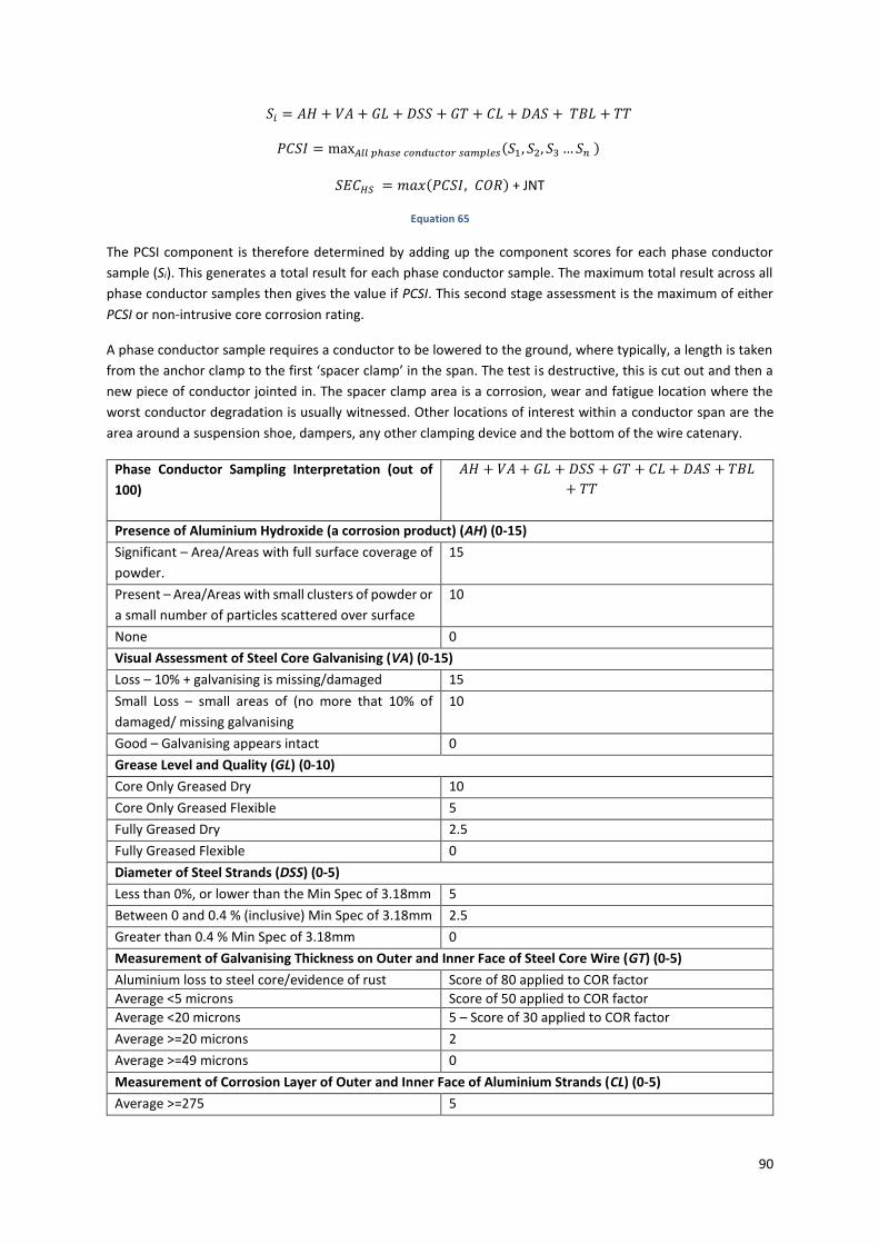
90

𝑆𝑖 = 𝐴𝐻 + 𝑉𝐴 + 𝐺𝐿 + 𝐷𝑆𝑆 + 𝐺𝑇 + 𝐶𝐿 + 𝐷𝐴𝑆 + 𝑇𝐵𝐿 + 𝑇𝑇

𝑃𝐶𝑆𝐼 = max𝐴𝑙𝑙 𝑝ℎ𝑎𝑠𝑒 𝑐𝑜𝑛𝑑𝑢𝑐𝑡𝑜𝑟 𝑠𝑎𝑚𝑝𝑙𝑒𝑠 (𝑆1, 𝑆2, 𝑆3…𝑆𝑛 )

𝑆𝐸𝐶𝐻𝑆 = 𝑚𝑎𝑥(𝑃𝐶𝑆𝐼, 𝐶𝑂𝑅) + JNT

Equation 65

The PCSI component is therefore determined by adding up the component scores for each phase conductor

sample (Si). This generates a total result for each phase conductor sample. The maximum total result across all

phase conductor samples then gives the value if PCSI. This second stage assessment is the maximum of either

PCSI or non-intrusive core corrosion rating.

A phase conductor sample requires a conductor to be lowered to the ground, where typically, a length is taken

from the anchor clamp to the first ‘spacer clamp’ in the span. The test is destructive, this is cut out and then a

new piece of conductor jointed in. The spacer clamp area is a corrosion, wear and fatigue location where the

worst conductor degradation is usually witnessed. Other locations of interest within a conductor span are the

area around a suspension shoe, dampers, any other clamping device and the bottom of the wire catenary.

Phase Conductor Sampling Interpretation (out of

100)

𝐴𝐻 + 𝑉𝐴 + 𝐺𝐿 + 𝐷𝑆𝑆 + 𝐺𝑇 + 𝐶𝐿 + 𝐷𝐴𝑆 + 𝑇𝐵𝐿

+ 𝑇𝑇

Presence of Aluminium Hydroxide (a corrosion product) (AH) (0-15)

Significant – Area/Areas with full surface coverage of

powder.

15

Present – Area/Areas with small clusters of powder or

a small number of particles scattered over surface

10

None 0

Visual Assessment of Steel Core Galvanising (VA) (0-15)

Loss – 10% + galvanising is missing/damaged 15

Small Loss – small areas of (no more that 10% of

damaged/ missing galvanising

10

Good – Galvanising appears intact 0

Grease Level and Quality (GL) (0-10)

Core Only Greased Dry 10

Core Only Greased Flexible 5

Fully Greased Dry 2.5

Fully Greased Flexible 0

Diameter of Steel Strands (DSS) (0-5)

Less than 0%, or lower than the Min Spec of 3.18mm 5

Between 0 and 0.4 % (inclusive) Min Spec of 3.18mm 2.5

Greater than 0.4 % Min Spec of 3.18mm 0

Measurement of Galvanising Thickness on Outer and Inner Face of Steel Core Wire (GT) (0-5)

Aluminium loss to steel core/evidence of rust Score of 80 applied to COR factor

Average <5 microns Score of 50 applied to COR factor

Average <20 microns 5 – Score of 30 applied to COR factor

Average >=20 microns 2

Average >=49 microns 0

Measurement of Corrosion Layer of Outer and Inner Face of Aluminium Strands (CL) (0-5)

Average >=275 5

91

Average >100 2

Average >0 0

Diameter of Aluminium Strands (DAS) (0-5)

Average >=275 5

Average >100 2

Average >0 0

Average Tensile Breaking Load of Outer Aluminium Strands (TBL) (0-20)

<1120N 20

>=1120N 15

>=1280N 10

>=1310N 0

Torsion Test (Average Revolutions to Failure of Outer Aluminium Strands (TT) (0-20)

<1 revolution to failure 20

>=1 revolution to failure 15

>=10 revolutions to failure 5

>=18 revolutions to failure 0

Table 36

Eddy current non-intrusive core corrosion rating measure the residual zinc coating of the steel core within ACSR.

These employ a device that is required to be mounted on and propelled down a conductor wire. Changes in

magnetic flux density detect loss of zinc and aluminium to the steel core.

Core Sample Interpretation Score (COR)

Aluminium loss detected 80

Residual zinc coating of 5 microns or less (‘Severe

Corrosion’)

50

Residual zinc coating of >5 to <=20 microns (‘Partial Corrosion’)

30

Minimum 0

Table 37

A ‘Joint’ factor is made up of a ‘Tate’ joint multiplier and infra red survey score.

A multiplier is assigned for OHL ‘Tate’ joints to reflect that this type of joint is inferior to a hexagonal

compression. If ‘Tate’ joints are present then TATE=2, otherwise 1.

Infra Red Survey Score

Hot Joints in Main Compression >2.5% of Tension Towers in last 5 years

10

Hot Joints in Compressed Jumper Palm >2.5% of

Tension Towers in last 5 years

7.5

Hot Joints in Bolted Jumper Palm >2.5% of Tension Towers in last 5 years

5

Table 38

92

8.2.5. OVERHEAD LINES FITTINGS PARAMETERS

Overhead Line Fittings are assigned an EOL modifier using a 2 stage calculation process. The first stage is

preliminary assessment based on age. The second stage is based on visual condition assessment (referred to as

a ‘Level 1’), an ‘outage’ or intrusive condition assessment (‘Level 2’), current defects and failure history.

Scoring assessments are made on sections of circuit that are typically homogenous in conductor type, installation

date and environment.

8.2.5.1 OHL FITTINGS FAILURE MODE GROUPING

OHL fitting assets are currently split into two different failure mode groups each of which has a different earliest

and latest onset of failure value, and therefore a different AAL. These groupings are Quad Conductor Routes and

Twin & Triple Conductor Routes.

8.2.5.2. OHL FITTINGS END OF LIFE MODIFIER

The formula to determine the EOL modifier of fittings is given below, and is capped at a maximum of 100.

𝐸𝑂𝐿𝑚𝑜𝑑 = max(𝑆𝑃𝐴, 𝐷𝐴𝑀, 𝐼𝑁𝑆, 𝑃𝐻𝐹)

Equation 66

A maximum score of spacers, dampers, insulators and phase fittings is applied, since the conditional probability

of the asset failing is determined by the weakest component. In this case the most deteriorated component is

the component that has the highest EOL modifier component score.

The components of this formula will all be broken down and described in more detail below. The meaning of

these components is:

1. Spacers (SPA)

2. Dampers (DAM)

3. Insulators (INS)

4. Phase Fittings (PHF). This category includes linkages (shackles, straps, dowel pins etc.) and Arcing

Horns/Corona Rings.

The score for the NOMS reporting unit is calculated as below for each component class (spacers, dampers,

insulators and phase fittings). It remains necessary to review the results for each tower and span across the

NOMs reporting unit level to understand the distribution of condition across the system. A targeted intervention

may be required within a component class or within a sub section of the OHL circuit or both. To guard against

the averaging effect of large routes masking specific sections requiring attention, a threshold volume of 4.5km

is used as below. This is equivalent to our smaller routes and is roughly three sections or 15 towers/spans. Our

research shows distinct operating environments can be localised to a span or section. It is likely that intervention

may be required on a small number of sections within a larger route.

The ‘asset’ below is defined as tower (for insulators, linkages and dampers) or span (spacers). Further

explanation on how to apply the logic in the criteria column of the table is explained below in the preliminary

assessment section.

93

Asset Health Score Criteria

0 >=50% of Assets or 4.5 circuit km are New Assets, Less than 5 years Old

10 >=50% of Assets or 4.5 circuit km scoring 10 or more









100 >=50% of Assets or 4.5 circuit km scoring 100

Table 39

8.2.5.3. PRELIMINARY ASSESSMENT

The Preliminary assessment of spacers, dampers, insulators and phase fittings is based on the age of the oldest

components versus the anticipated life. The preliminary score for each of these components (𝑆𝑃𝐴𝑃𝑅𝐸 , 𝐷𝐴𝑀𝑃𝑅𝐸

, 𝐼𝑁𝑆𝑃𝑅𝐸 , 𝑃𝐻𝑆𝑃𝑅𝐸 ) can be determined from the table below.

𝑆𝑃𝐴𝑃𝑅𝐸 , 𝐷𝐴𝑀𝑃𝑅𝐸 , 𝐼𝑁𝑆𝑃𝑅𝐸 , 𝑃𝐻𝑆𝑃𝑅𝐸 = {0 𝐴𝐺𝐸 − 𝐴𝐴𝐿 ≤ −13300 𝐴𝐺𝐸 − 𝐴𝐴𝐿 ≥ −3

30(𝐴𝐺𝐸 − 𝐴𝐴𝐿) + 390 𝑜𝑡ℎ𝑒𝑟𝑤𝑖𝑠𝑒

Equation 67

8.2.5.4. LEVEL 1 AND LEVEL 2 CONDITION ASSESSMENT

Each of the categories, spacers, dampers, insulators and phase fittings are assessed against condition

statements. Each of these statements has a weighting which results in the overall End of Life modifier.

Level 1 is a visual condition assessment of fittings components. The usual method of data collection is by High

Definition Camera mounted to a helicopter.

Level 2 is an ‘outage’ or ‘intrusive’ condition assessment. This extra degree of inspection is required on those

components likely to produce ‘false negative‘ or ‘false positive’ results when the level 1 approach is adopted.

This includes wear to phase fittings and loss of dielectric strength in insulation. Only some of the components

have level 2 information.

94

8.2.5.5. SPACERS

𝑆𝑃𝐴 =(𝑆𝑃𝐴𝑃𝑅𝐸 ∗ 𝐿𝑉𝐿1) + 𝑆𝑃𝐴𝑂𝑣𝐶𝐴

6

Equation 68

Where:

SPA is the overall spacer score

𝑆𝑃𝐴𝑃𝑅𝐸 is the preliminary spacer score

LVL1 is a multiplier: if Level 1 condition assessment is available (=0), if Level 1 condition assessment is not

available (=1)

𝑆𝑃𝐴𝑂𝑣𝐶𝐴 is the overall Condition Assessment score for spacers which is a function of the % of assets falling into

scores 0-100 following Level 1 condition assessment(SPALV1), Level 2 condition assessment from the route

(SPALV2), latest defects from annual foot patrols (SPACDEF) and failures(SPAFAIL). These are then multiplied by an

operating environment modifier.

To calculate 𝑆𝑃𝐴𝑂𝑣𝐶𝐴 on NOMs Reporting Unit Level:

An SPACA score is first calculated for all assets in each NOMs unit as described below. The 𝑆𝑃𝐴𝑂𝑣𝐶𝐴 value is then

given by the maximum of:

a) The score where 50% or more of assets in that NOMs unit have this SPACA score.

b) The maximum SPACA score is obtained from circuits that are 4.5km or longer.

For an individual spans:

𝑆𝑃𝐴𝐶𝐴 =max (𝑆𝑃𝐴𝐿𝑉𝐿1,𝑆𝑃𝐴𝐿𝑉𝐿2,𝑆𝑃𝐴𝐶𝐷𝐸𝐹,𝑆𝑃𝐴𝐹𝐴𝐼𝐿)

6∗ (𝐸𝑁𝑉𝑀𝑂𝐷)

Equation 69

where:

𝑆𝑃𝐴𝐹𝐴𝐼𝐿 where ≥2.5% of population of family on the route has failed in last five years

ENVMOD =

{

1.2 𝑖𝑓 𝐴1.1 𝑖𝑓 𝐵1 𝑖𝑓 𝐶

1.2 𝑖𝑓 𝐷1 𝑖𝑓 𝑛𝑜𝑡 𝐴, 𝐵, 𝐶 𝑜𝑟 𝐷

where:

95

Environment Modifier Description

A Heavy Pollution – 5 km of a coast or major estuary, or within 10km downwind of an older, low stack coal fired power station or adjacent to chemical

plant.

B Some Pollution – 5-15km from a coast or major estuary or in an industrial area or on high ground

downwind of pollution source

C No Pollution – Rural areas at least 15km from the coast

D Wind Exposed – High ground >150 metres above sea level, or areas with known sub-conductor oscillation

and/or galloping problems

Table 40

SPACER VISUAL CONDITION STATEMENTS SPALVL1 & SPACDEF

Spacers Good

Condition Dull

Appearance Black

Appearance

Slight Oxidation Deposits Around Conductor Clamp and Locking Pins

Severe Oxidation Deposits Around Conductor Clamp and Locking Pins

Tight and Secure 100 200 300 400 500

Locking Pins Ineffective or Loose

600 600 600 600 600

Rubber Missing 600 600 600 600 600

Loose Arms 600 600 600 600 600

Clamps Loose 600 600 600 600 600

Clamps Open 600 600 600 600 600

Missing 600 600 600 600 600

Table 41

96

SPACER INTRUSIVE CONDITION STATEMENTS SPALVL2

Conductor Samples

from Spacer Families on the Same Route and

Environment

Good Condition

Dull Appearance

Black Appearance

Slight Oxidation Deposits Around Conductor Clamp and Locking Pins

Severe Oxidation Deposits Around Conductor Clamp and Locking Pins

Galvanic Corrosion between Rubber and Aluminium

Tensile Breaking Load <1310N but >=1114N Torsion Fail 5-15 Revs

Tensile Breaking Load <1114N Torsion Failure <5 Revs

Flattening/ Deformation of Conductor Wire

300 300 400 500 600 600 400 500

Heavy Fretting of Conductor Wires (>=50% of wire area indented in any layer)

300

300

400

500

600

600

400

500

Broken Conductor Wires

600 600 600 600 600 600 600 600

Table 42

8.2.5.6. DAMPERS

𝐷𝐴𝑀 =(𝐷𝐴𝑀𝑃𝑅𝐸 ∗ 𝐿𝑉𝐿1) + 𝐷𝐴𝑀𝑂𝑣𝐶𝐴

6

Equation 70

where:

DAM is the overall damper score

𝐷𝐴𝑀𝑃𝑅𝐸 is the preliminary damper score


available (=1)

There is no Level 2 stage assessment for dampers.

𝐷𝐴𝑀𝑂𝑣𝐶𝐴 is the overall condition assessment score for dampers which is a function of the % of assets falling into

scores 0-100 following Level 1 condition assessment, latest defects from annual foot patrols and failures. These

are then multiplied by an operating environment modifier.

To calculate 𝐷𝐴𝑀𝑂𝑣𝐶𝐴 on NOMs Reporting Unit Level:

An DAMCA score is first calculated for all assets in each NOMs unit as described below. The 𝐷𝐴𝑀𝑂𝑣𝐶𝐴 value is

then given by the maximum of:

a) The score where 50% or more of assets in that NOMs unit have this DAMCA score.

b) The maximum DAMCA score is obtained from circuits that are 4.5km or longer.

97

For an Individual Span:

𝐷𝐴𝑀𝐶𝐴 =max (𝐷𝐴𝑀𝐿𝑉𝐿1, 𝐷𝐴𝑀𝐶𝐷𝐸𝐹 , 𝐷𝐴𝑀𝐹𝐴𝐼𝐿)


Equation 71

where:

𝐷𝐴𝑀𝐹𝐴𝐼𝐿 where ≥2.5% of population of family on the route has failed in last five years

ENVMOD =

{



where:



plant.






Table 43

DAMPER VISUAL CONDITION STATEMENTS DAMLVL1& DAMCDEF

Damper Galvanising Weathered, Dull Appearance

Galvanised Coating Starting to Deteriorate

Light Rust, Majority of Galvanised Coating Missing

Heavy Rust Heavy Corrosion, Pitting of Steelwork and Some Section Loss

0-20° Droop 100 100 200 200 300

20°-40° Droop

100 100 200 300 400

40° + Droop 600 600 600 600 600

Bell(s) missing, messenger wire broken or slipped

600 600 600 600 600

98

Slipped 600 600 600 600 600

Missing 600 600 600 600 600

Table 44

8.2.5.7. INSULATORS

𝐼𝑁𝑆 =(𝐼𝑁𝑆𝑃𝑅𝐸 ∗ 𝐿𝑉𝐿1) + 𝐼𝑁𝑆𝑂𝑣𝐶𝐴

6

Equation 72

Where:

INS is the overall insulator score

𝐼𝑁𝑆𝑃𝑅𝐸 is the preliminary insulator score


available (=1)

𝐼𝑁𝑆𝑂𝑣𝐶𝐴 is the overall condition assessment score for insulators which is a function of the % of assets falling into

scores 0-100 following Level 1 condition assessment, Level 2 condition assessment from the route, latest defects

from annual foot patrols and failures. These are then multiplied by an operating environment modifier.

To calculate 𝐼𝑁𝑆𝑂𝑣𝐶𝐴 on NOMs Reporting Unit Level:

An INSCA score is first calculated for all assets in each NOMs unit as described below. The 𝐼𝑁𝑆𝑂𝑣𝐶𝐴 value is then


a) The score where 50% or more of assets in that NOMs unit have this INSCA score.

b) The maximum INSCA score is obtained from circuits that are 4.5km or longer.


𝐼𝑁𝑆𝐶𝐴 =max (𝐼𝑁𝑆𝐿𝑉𝐿1, 𝐼𝑁𝑆𝐿𝑉𝐿2, 𝐼𝑁𝑆𝐶𝐷𝐸𝐹 , 𝐼𝑁𝑆𝐹𝐴𝐼𝐿)


Equation 73

where:

𝐼𝑁𝑆𝐹𝐴𝐼𝐿 where ≥2.5% of population of family on the route has failed in last five years

ENVMOD =

{



where:

99



plant.






Table 45

INSULATOR VISUAL CONDITION ASSESSMENT 𝐼𝑁𝑆𝐿𝑉𝐿1& INSCDEF

Insulator

Galvanising Weathered,

Dull Appearance


Light Rust on Bells, Majority of Galvanised

Coating Missing

Heavy Rust on Bells

Bells Severely Corroded and Some Section

Loss

No Pollution 100 200 200 300 300

Evidence of Light

Pollution 200 300 300 300 400

Evidence of Heavy

Pollution 300 300 300 300 400

Visible Burn Marks

400 400 500 500 500

Evidence of Crazing

600 600 600 600 600

Table 46

INSULATOR INTRUSIVE CONDITION ASSESSMENT 𝐼𝑁𝑆𝐿𝑉𝐿2& INSCDEF

Insulator Resistance Testing from Insulator Families on the Same Route and Environment

Galvanising Weathered, Dull Appearance


Light Rust on Bells, Majority of Galvanised Coating Missing

Heavy Rust on Bells

Bells Severely Corroded and Some Section Loss to Pins <10% for 190kN <2.5% for 300kN

Loss of Steel Pin Area 10% for 190KN, 2.5% for 300kN

Loss of Steel Pin Area 40% for 190KN, 10% for 300kN

Evidence of Failed units

100

but string or set do not meet 'failed' criteria of 3 in a single string or 6 in a bundle

300

300

300

400

400

500

500

A single String or Set fails Meggar Test Criteria (3 in a string or 6 in a bundle)

600

600

600

600

600

600

600

Table 47

8.2.5.8. PHASE FITTINGS

𝑃𝐻𝐹 =(𝑃𝐻𝐹𝑃𝑅𝐸 ∗ 𝐿𝑉𝐿1) + 𝑃𝐻𝐹𝑂𝑣𝐶𝐴

6

Equation 74

Where:

PHF is the overall phase fittings score

𝑃𝐻𝐹𝑃𝑅𝐸 is the preliminary phase fittings score


available (=1)

𝑃𝐻𝐹𝑂𝑣𝐶𝐴 is the overall condition assessment score for phase fittings which is a function of the % of assets falling

into scores 0-100 following Level 1 condition assessment, Level 2 condition assessment from the route, latest

defects from annual foot patrols and failures. These are then multiplied by an operating environment modifier.

To calculate 𝑃𝐻𝐹𝑂𝑣𝐶𝐴 on NOMs Reporting Unit Level:

An PHFCA score is first calculated for all assets in each NOMs unit as described below. The 𝑃𝐻𝐹𝑂𝑣𝐶𝐴 value is then


a) The score where 50% or more of assets in that NOMs unit have this PHFCA score.

b) The maximum PHFCA score is obtained from circuits that are 4.5km or longer.


𝑃𝐻𝐹𝐶𝐴 =max (𝑃𝐻𝐹𝐿𝑉𝐿1, 𝑃𝐻𝐹𝐿𝑉𝐿2, 𝑃𝐻𝐹𝐶𝐷𝐸𝐹 , 𝑃𝐻𝐹𝐹𝐴𝐼𝐿)


Equation 75

where:

𝑃𝐻𝐹𝐹𝐴𝐼𝐿 where ≥2.5% of population of family on the route has failed in last five years

101

ENVMOD =

{



where:

Enviroment Modifier Description

A Heavy Pollution – 5 km of a coast or major estuary, or within 10km downwind of an older, low stack coal

fired power station or adjacent to chemical plant.






Table 48

𝑃𝐻𝐹𝐿𝑉𝐿1 is the Level 1 Condition Assessment score for phase fittings.

𝑃𝐻𝐹𝐿𝑉𝐿2 is the Level 2 Condition Assessment score for phase fittings.

Phase Fittings are made up of

1. Suspension Linkages: Shackle, Ball Ended Eye Link, Yoke Plate, Shoes, Maintenance Bracket, Weights,

Straps. (𝐿𝑁𝐾𝑆𝑈𝑆)

2. Tension Linkages: Landing Pin, Shackle, Ball Ended Eye Link, Straps, Yoke Plate. (𝐿𝑁𝐾𝑇𝐸𝑁)

3. Arcing Horns and Corona Rings. (ARC)

4. Dowel Pins and Bolts. (DOW)

𝑃𝐻𝐹𝐿𝑉𝐿1 = max ((𝑚𝑎𝑥(𝐿𝑁𝐾𝑆𝑈𝑆)), (𝑚𝑎𝑥(𝐿𝑁𝐾𝑇𝐸𝑁)), 𝐴𝑅𝐶, 𝐷𝑂𝑊)

Equation 76

𝑃𝐻𝐹𝐿𝑉𝐿2 = max ((𝑚𝑎𝑥(𝐿𝑁𝐾𝑆𝑈𝑆)), (𝑚𝑎𝑥(𝐿𝑁𝐾𝑇𝐸𝑁)), 𝐷𝑂𝑊)

Equation 77

The max(LNKSUS) means maximum of all suspension linkages on the tower. Max(LNKTEN) means maximum of all

tension linkages on the tower. There is no Level 2 assessment for Arcing Horns and Corona Rings

These have their own set of condition statements and scores as set out below.

102

𝑃𝐻𝐹𝐿𝑉𝐿1 & PHFCDEF SUSPENSION AND TENSION LINKAGES, DOWEL PINS AND BOLTS

Phase and Earthwire Fittings (Suspension & Tension), Dowel Pins and Bolts





Minimal Wear 0-10%

100 200 300 300 400

Slight Wear 10-20%

200 300 300 400 500

Moderate Wear 20-40%

300 300 400 500 500

Heavy Wear 40-60%

400 400 500 600 600

Severe Wear >60%

600 600 600 600 600

Table 49

𝑃𝐻𝐹𝐿𝑉𝐿1 & PHFCDEF ARCING HORNS AND CORONA RINGS

Arcing Horn/ Corona Ring





Tight and Secure

100 200 300 400 500

Missing Components, Locking Nuts etc

300 400 400 400 500

Loose 400 400 500 500 500

Missing 600 600 600 600 600

Incorrect Length

600 600 600 600 600

Table 50

𝑃𝐻𝐹𝐿𝑉𝐿2 & PHFCDEF SUSPENSION AND TENSION LINKAGES, DOWEL PINS AND BOLTS

Intrusive assessment of Linkages from the same route and environment

Material Loss of Steel through corrosion < 20% Cross Sectional Area

Material Loss of Steel through corrosion >= 20% Cross Sectional Area

Material Loss of Steel through corrosion >= 40% Cross Sectional Area

Minimal Wear 0-10% 300 400 600

Slight Wear 10-20% 400 500 600

Moderate Wear 20-40% 500 600 600

Heavy Wear 40-60% 600 600 600

103

Severe Wear >60% 600 600 600

Missing/ Out of Plumb >200/ Cracked Wedge Clamp

600 600 600

Table 51

8.2.5.9. OVERALL END OF LIFE MODIFIER FOR OHL FITTINGS

The end of life modifier formula for fittings given at the beginning of this section is reproduced below with a

mathematic summary of how each component is determined.

𝑬𝑶𝑳𝒎𝒐𝒅 = 𝐦𝐚𝐱(𝑺𝑷𝑨,𝑫𝑨𝑴, 𝑰𝑵𝑺, 𝑷𝑯𝑭)

Equation 78

Where:

𝑆𝑃𝐴 =(𝑆𝑃𝐴𝑃𝑅𝐸 ∗ 𝐿𝑉𝐿1) + 𝑆𝑃𝐴𝑂𝑣𝐶𝐴

6

Equation 79

𝐷𝐴𝑀 =(𝐷𝐴𝑀𝑃𝑅𝐸 ∗ 𝐿𝑉𝐿1) + 𝐷𝐴𝑀𝑂𝑣𝐶𝐴

6

Equation 80

𝐼𝑁𝑆 =(𝐼𝑁𝑆𝑃𝑅𝐸 ∗ 𝐿𝑉𝐿1) + 𝐼𝑁𝑆𝑂𝑣𝐶𝐴

6

Equation 81

𝑃𝐻𝐹 =(𝑃𝐻𝐹𝑃𝑅𝐸 ∗ 𝐿𝑉𝐿1) + 𝑃𝐻𝐹𝑂𝑣𝐶𝐴

6

Equation 82

The overall condition assessment (OvCA) is determined from the underlying condition assessment (CA) for each

span according to the logic described above.

For an Individual Span the condition assessment score is determined from the following formula:

𝑆𝑃𝐴𝐶𝐴 =max (𝑆𝑃𝐴𝐿𝑉𝐿1, 𝑆𝑃𝐴𝐿𝑉𝐿2, 𝑆𝑃𝐴𝐶𝐷𝐸𝐹 , 𝑆𝑃𝐴𝐹𝐴𝐼𝐿)


Equation 83

𝐷𝐴𝑀𝐶𝐴 =max (𝐷𝐴𝑀𝐿𝑉𝐿1, 𝐷𝐴𝑀𝐶𝐷𝐸𝐹 , 𝐷𝐴𝑀𝐹𝐴𝐼𝐿)


Equation 84

𝐼𝑁𝑆𝐶𝐴 =max (𝐼𝑁𝑆𝐿𝑉𝐿1, 𝐼𝑁𝑆𝐿𝑉𝐿2, 𝐼𝑁𝑆𝐶𝐷𝐸𝐹 , 𝐼𝑁𝑆𝐹𝐴𝐼𝐿)


Equation 85

104

𝑃𝐻𝐹𝐶𝐴 =max (𝑃𝐻𝐹𝐿𝑉𝐿1, 𝑃𝐻𝐹𝐿𝑉𝐿2, 𝑃𝐻𝐹𝐶𝐷𝐸𝐹 , 𝑃𝐻𝐹𝐹𝐴𝐼𝐿)


Equation 86

national grid electricity transmission network …...fam family weighting score for overhead line...

Documents