MUTI-METRIC ADAPTIVE ROUTING ALGORITHM

FOR UNDERWATER WIRELESS SENSOR NETWORKS

A Thesis

by

BHANU KISHORE KAMAPANTULA

Submitted in Partial Fulfillment of the Requirements for the Degree of

MASTER OF SCIENCE

Texas A&M University - Corpus Christi

Corpus Christi, Texas

August 2011

Major Subject: Computer Science

iii

ABSTRACT

Research in Underwater Wireless Sensor Networks (UWSNs) has flourished in

recent past. Routing in underwater wireless sensor networks differs from routing in

terrestrial wireless sensor networks. This is due to issues such as limited bandwidth in

water, node mobility due to water currents, and potential delay in data packet trans-

mission. A novel Multi-Metric Adaptive Routing (MMAR) algorithm for UWSNs is

proposed and implemented. MMAR algorithm considers depth at which nodes are

deployed, packet age, energy level at each node, average energy level of the network at

a given instance, and hop count from a particular participating node to the base node.

The metrics level at every node is estimated using a vector representation. A routing

technique is chosen depending on the value of calculated metrics. The three possibili-

ties of routing techniques that can be adapted are Almost-Ring approach, Distributed

approach, or Centralized approach. Base node floats on water surface and participat-

ing nodes are deployed underwater. MMAR routing implements acoustic and radio

energy models for communication underwater and over the air, respectively. The rout-

ing algorithm is simulated in C language and Message Passing Interface (MPI). A case

study on forecasting red tides using wireless sensor networks is presented to establish

the centralized routing approach. The performance of different routing strategies is

noted apart from determining the energy required by a node to transmit and receive

data from other nodes. The performance of MMAR is compared with Vector-Based

Forwarding and Depth-Based Routing techniques. The overall performance of the

Multi-Metric Adaptive Routing algorithm is average considering that node mobility

is not addressed.

iv

DEDICATION

I would like to dedicate this research work to my parents, Satyanarayana Murthy

and Krishna Kumari, and my grandmother Bala Tripura Sundari. My ability to

question whatever I come across is only because of the freedom my parents gave me

since my childhood. I owe my disciplined life to my grandmother who took great

pains to nurture me.

v

Page

ACKNOWLEDGEMENTS

It is a great pleasure for me to acknowledge all without whom, this thesis would

not have seen the daylight. I would like to acknowlege my advisor Dr. Ahmed Mahdy

who has been a guiding force in my research. He has been very enthusiastic about my

progress academically and has taken keen interest in nurturing my research interests.

For two years, my interactions with him have been rewarding and enriching. Without

a doubt, he is the best mentor for Master’s degree one can come across.

I would like to thank Dr. Dulal Kar, Dr. Longzhuang Li and Dr. Mufid Abudiab

for serving on my Thesis committee. I worked with Dr. Kar and Dr. Li in Summer

2010, 2011 for the summer REU program where I had an unique opportunity to

interact and work with undergraduate students. I am extremely thankful for their

support at TAMUCC.

I would like to thank Dr. King for his valuable advice and for the wonderful

discussions we had. His teachings offered me a new perspective to address Computer

Science problems.

I would like to acknowledge the support of my friends Santosh, LKC, Shravan,

Ashu, Sanketh, Karteek, Bharath, Pavan, Doctor Bharath, Vishnu, Sireesha who

always believed in me. I am grateful for the time spent with Sowmya, Sandeep, Raj,

Rakesh, Vinay, Sushil bhai, Geetha and Sharath at Corpus Christi. I would like to

acknowledge the support of Ramakrishna Podila for his invaluable suggestions on

research. I am grateful to Rakesh Tatiparthy and Sai Krishna Majeti for the support

they offered me when I needed it the most.

I am extremely thankful for the support of my brother, Sunder Nagesh, who has

been an instrumental, invisible and inspirational force behind my success.

vi

TABLE OF CONTENTS

CHAPTER Page

ABSTRACT . . . . . . . . . . . . . . . . . . . . . . . . . . . . . . . . . . iii

DEDICATION . . . . . . . . . . . . . . . . . . . . . . . . . . . . . . . . . iv

ACKNOWLEDGMENTS . . . . . . . . . . . . . . . . . . . . . . . . . . . v

TABLE OF CONTENTS . . . . . . . . . . . . . . . . . . . . . . . . . . . vi

LIST OF TABLES . . . . . . . . . . . . . . . . . . . . . . . . . . . . . . viii

LIST OF FIGURES . . . . . . . . . . . . . . . . . . . . . . . . . . . . . . ix

1 INTRODUCTION . . . . . . . . . . . . . . . . . . . . . . . . . . 1

1.1 Background . . . . . . . . . . . . . . . . . . . . . . . . . . 1

1.2 Challenges in Underwater Wireless Sensor Networks . . . . 3

1.3 Contribution . . . . . . . . . . . . . . . . . . . . . . . . . . 7

2 LITERATURE REVIEW . . . . . . . . . . . . . . . . . . . . . . 10

2.1 RF Electromagnetic Communication in UWSNs . . . . . . 10

2.2 Delay/Disruption Tolerant Networks . . . . . . . . . . . . 11

2.3 GPS-free Routing Protocol . . . . . . . . . . . . . . . . . . 11

2.4 E-PULRP . . . . . . . . . . . . . . . . . . . . . . . . . . . 12

2.5 MAC Protocol for Data Collection . . . . . . . . . . . . . . 13

2.6 Energy-Aware Routing Protocol . . . . . . . . . . . . . . . 13

2.7 Vector-Based Forwarding Protocol . . . . . . . . . . . . . . 14

2.8 Hop-by-Hop Vector-Based Forwarding . . . . . . . . . . . . 15

3 MULTI-METRIC ADAPTIVE ROUTING ALGORITHM . . . . 17

3.1 Network Topology . . . . . . . . . . . . . . . . . . . . . . . 17

3.2 Attributes Used . . . . . . . . . . . . . . . . . . . . . . . . 18

3.3 Routing Approaches . . . . . . . . . . . . . . . . . . . . . 19

3.4 Multi-Metric Adaptive Routing Algorithm . . . . . . . . . 20

3.5 Energy Model . . . . . . . . . . . . . . . . . . . . . . . . . 25

3.6 Event Synchronization . . . . . . . . . . . . . . . . . . . . 26

vii

CHAPTER Page

3.7 Multi-Metric Adaptive Routing Algorithm Complexity . . 27

3.7.1 Complexity of Centralized Routing Approach . . . . 27

3.7.2 Complexity of Almost-ring Routing Approach . . . 28

3.7.3 Complexity of Distributed Routing Approach . . . . 28

3.7.4 Complexity of Multi-Metric Adaptive Routing

Algorithm . . . . . . . . . . . . . . . . . . . . . . . 28

3.7.5 Communication Overhead . . . . . . . . . . . . . . 29

3.7.5.1 Number of Messages . . . . . . . . . . . . . . 29

3.7.5.2 Best and Worst-Case Scenarios . . . . . . . . 30

3.7.6 Best-Case Scenario . . . . . . . . . . . . . . . . . . 31

3.7.6.1 Energy Constraints . . . . . . . . . . . . . . 31

3.7.6.2 Time Complexity . . . . . . . . . . . . . . . 31

3.7.7 Worst-Case Scenario . . . . . . . . . . . . . . . . . 32

3.8 Overall Characteristics of Multi-Metric Adaptive Rout-

ing Algorithm . . . . . . . . . . . . . . . . . . . . . . . . . 32

4 CASE STUDY - FORECASTING RED TIDES USING UN-

DERWATER WIRELESS SENSOR NETWORKS . . . . . . . . 34

4.1 Current Approaches to Monitor Red Tides . . . . . . . . . 34

4.2 Contributing Factors . . . . . . . . . . . . . . . . . . . . . 36

4.3 Forecasting Red Tides Using Underwater Wireless Sen-

sor Networks . . . . . . . . . . . . . . . . . . . . . . . . . . 39

4.3.1 Simulating Red Tide Environment - Using TinyDB,

TOSSIM . . . . . . . . . . . . . . . . . . . . . . . . 39

4.3.1.1 Limitations of Forecasting Red Tides Us-

ing TinyDB and TOSSIM . . . . . . . . . . . 40

4.3.2 Simulating Red Tide Environment - Using C lan-

guage, Message Passing Interface . . . . . . . . . . . 42

5 PERFORMANCE EVALUATION . . . . . . . . . . . . . . . . . 44

5.1 Implementation . . . . . . . . . . . . . . . . . . . . . . . . 44

5.1.1 Centralized Algorithm Implementation . . . . . . . 44

5.1.2 Almost-Ring Algorithm Implementation . . . . . . . 45

5.1.3 Distributed Algorithm Implementation . . . . . . . 45

5.2 Simulation Results . . . . . . . . . . . . . . . . . . . . . . 48

5.2.1 Time Taken by Participating Nodes to Send In-

formation to the Base Node . . . . . . . . . . . . . 48

viii

CHAPTER Page

5.2.1.1 Time Calculation - Three Node Network

Simulation . . . . . . . . . . . . . . . . . . . 50

5.2.1.2 Time Calculation - Five Node Network

Simulation . . . . . . . . . . . . . . . . . . . 50

5.2.1.3 Time Calculation - Fifteen Node Network

Simulation . . . . . . . . . . . . . . . . . . . 51

5.2.1.4 Time Calculation - Fifty Node Network

Simulation . . . . . . . . . . . . . . . . . . . 52

5.3 Energy Analysis . . . . . . . . . . . . . . . . . . . . . . . . 53

5.3.1 Factors to Consider for Energy Analysis . . . . . . . 56

5.3.2 Energy Analysis of Centralized Routing Approach . 56

5.3.3 Energy Analysis of Almost-Ring and Distributed

Routing Approach . . . . . . . . . . . . . . . . . . . 57

5.4 Comparison to Other UWSN Routing Algorithms . . . . . 58

5.4.1 MMAR Performance Comparison with DBR and

VBF Protocols . . . . . . . . . . . . . . . . . . . . . 61

6 FUTURE RESEARCH DIRECTIONS . . . . . . . . . . . . . . 64

7 CONCLUSION . . . . . . . . . . . . . . . . . . . . . . . . . . . 68

REFERENCES . . . . . . . . . . . . . . . . . . . . . . . . . . . . . . . . . . 70

APPENDIX A . . . . . . . . . . . . . . . . . . . . . . . . . . . . . . . . . . . 76

APPENDIX B . . . . . . . . . . . . . . . . . . . . . . . . . . . . . . . . . . . 78

7.1 Distributed Routing Approach . . . . . . . . . . . . . . . . 79

7.2 Almost-Ring Routing Approach . . . . . . . . . . . . . . . 80

7.3 Energy and Metrics Calculations . . . . . . . . . . . . . . . 80

ix

LIST OF TABLES

TABLE Page

I Speeds of Different Waves . . . . . . . . . . . . . . . . . . . . . . . . 4

II Different Scenarios for Algorithmic Complexities . . . . . . . . . . . 29

III Number of Messages Involved in Different Routing Strategies . . . . 30

IV Categorized Group Values of Contributing Factors . . . . . . . . . . 40

V Contributing Factors and Corresponding Threshold Range . . . . . . 43

VI Number of Nodes Per Level - Four Levels Description . . . . . . . . . 46

VII Node Number and Corresponding Constant Values . . . . . . . . . . 48

VIII Variables Implemented and Corresponding Description . . . . . . . . 49

IX Node Number, Time Taken to Transmit Packet to Base Node - 3 Nodes 50

X Node Number, Time Taken to Transmit Packet to Base Node - 5 Nodes 50

XI Node Number, Time Taken to Transmit Packet to Base Node - 15 Nodes 51

XII Node Number, Time Taken to Transmit Packet to Base Node - 50 Nodes 52

XIII Different Variables Attributed to a Participating Node, Assigned Values 57

XIV Comparison of Different UWSN Routing Algorithms . . . . . . . . . 59

XV Percentage of Energy Consumed by Nodes in Centralized Routing

Approach . . . . . . . . . . . . . . . . . . . . . . . . . . . . . . . . . 59

XVI Percentage of Energy Consumed by Nodes - Almost-Ring Routing

Approach . . . . . . . . . . . . . . . . . . . . . . . . . . . . . . . . . 59

XVII Dependence of Performance of Routing Approaches on Factors Involved 60

XVIII Comparing DBR, MMAR and VBF . . . . . . . . . . . . . . . . . . . 62

x

LIST OF FIGURES

FIGURE Page

1 Centralized Routing Approach . . . . . . . . . . . . . . . . . . . . . 20

2 Distributed Routing Approach . . . . . . . . . . . . . . . . . . . . . 21

3 Almost-Ring Routing Approach . . . . . . . . . . . . . . . . . . . . . 21

4 Multi-metric Adaptive Routing Algorithm . . . . . . . . . . . . . . . 23

5 Red Tides . . . . . . . . . . . . . . . . . . . . . . . . . . . . . . . . . 35

6 Simulation of Estimation Oxygen - Forecasting Red Tides Using

TinyDB, TOSSIM . . . . . . . . . . . . . . . . . . . . . . . . . . . . 41

7 Communication in Distributed Routing Approach . . . . . . . . . . . 47

8 Time Observations (Seconds) for Centralized Routing Approach . . . 53

9 Time Observations (Seconds) for Centralized and Almost-Ring

Routing Approaches . . . . . . . . . . . . . . . . . . . . . . . . . . . 54

10 Time Observations (Seconds) for Centralized and Distributed Rout-

ing Approaches . . . . . . . . . . . . . . . . . . . . . . . . . . . . . . 55

11 Relation of Packet Age to Energy Required Per Packet . . . . . . . . 58

12 Increase in Energy Consumption with Packet Age . . . . . . . . . . . 60

13 Number of Messages to Initialize Protocol - 5 nodes . . . . . . . . . . 63

1

CHAPTER 1

INTRODUCTION

1.1 Background

The field of Wireless Sensor Networks (WSNs) has captured the imagination of

the world with their potential to enhance human lives. WSNs have promised so much

that extensive research now is underway leading to wide applications of WSNs in

fields like agriculture monitoring, industrial monitoring, smart housing, automobile

industry and in civilian and military applications. A wireless sensor node is capable

of sensing information, processing, and transmitting information to other nodes via

proper communication. While sensor nodes have been developed for deployment on

land, native nodes for underwater environment have not been developed yet. Ter-

restrial nodes enclosed in specially designed cases have been deployed the nodes in

water but they do not exploit underwater conditions. These waterproof nodes are vul-

nerable to issues such as localization, communication overhead (i.e. electromagnetic

waves are susceptible over long distances in underwater environment), bandwidth,

dynamic topology, and node mobility. Hence, using nodes enclosed in cases is not

an ideal solution to monitor the underwater environment and is not suggested for

deployment in underwater environments. The field of Underwater Wireless Sensor

Networks (UWSNs) is established fairly recent with increased focus on underwater

surveillance and other military purposes. UWSNs potentially have wide range of ap-

plications in military, ocean environment conservation, and target tracking. UWSNs

are also useful in disaster management and monitoring earthquakes in underwater en-

vironments. Significant research has been invested currently in UWSNs considering

2

the potential of underwater applications [1, 2, 3].

Research prototypes of WSNs have been developed in academic institutions in

collaboration with industry. Some notable platforms of WSNs are MICAZ, MICA2,

TelOsb and IRIS. These nodes require sensor boards such as MTS300 and MTS300

for capturing temperature, acceleration among other measurement. MTS300 sen-

sor board is capable of measuring temperature, light and sound readings. MTS310

board, in addition to MTS300 abilities, is capable of observing accelerometer and

magnetometer readings.

Recent reports reveal researchers’ interest to explore dynamically reconfigurable

Marine Wireless Sensor Networks (MWSNs) [4]. This research aims to focus on sen-

sor mobility and dynamically changing network topology. The researchers also aim

to open new research directions which often lead to more exciting applications in

UWSNs. Project NEPTUNE aims to build an underwater ocean observatory net-

work that connects to the Internet from underwater environment [5]. This research

evidently opens an unknown underwater world. Interdisciplinary research has great

scope with possible collaborations among geological, computational and biological

sciences. Monitoring earthquakes and Tsunamis will be possible with assistance from

NEPTUNE. Ocean surveillance and monitoring marine species will be feasible with

NEPTUNE.

Building a robust UWSN requires the network to be secure, reliable and well con-

nected. An UWSN must be made safe and secure by lightweight (in terms of energy)

security protocols due to energy constraints in maintaining a power-inefficient secu-

rity protocols. The network must be intact even in cases of node deaths (total battery

usage), interruptions (change in network topology), or attacks (network/nodes can

be attacked to destroy or manipulate information at the nodes). Routing strategies

must be developed to hold the network together. Routing heavily depends on energy

3

levels available at the nodes. Routing in UWSNs is a challenge due to several reasons

[6]. Routing algorithms available for terrestrial WSNs are not suitable for UWSNs

due to critical differences in communication, localization, time synchronization, node

mobility, and power consumption.

1.2 Challenges in Underwater Wireless Sensor Networks

Underwater Wireless Sensor Networks are not void of problems and challenges.

Significant issues in UWSNs include communication, security, localization, energy,

node mobility, dynamic network topology, and routing.

UWSNs are extremely useful in military and enemy surveillance applications.

Securing information is critical in such applications. However, given the scarce power

resources available to the nodes deployed underwater, the entire process of encryption

and decryption (several rounds of mathematical operations) is power intense and

leaves node power-drained.

1. Communication

Terrestrial WSNs use radio energy model to communicate among nodes. Elec-

tromagnetic waves cannot travel over a long distance in underwater environ-

ments due to signal dampening. Alternative communication techniques to RF

(Radio Frequency) include acoustic communications and optical communica-

tions. A signal dampens (reduces) over time during signal propagation. Acous-

tic communication is widely used for underwater communication due to low

signal dampening in water. This approach works well especially in deep ocean

water. In shallow water, however, this mode of communication is disturbed by

temperature gradients, surface noise and multipath propagation due to reflec-

tion and refraction [7]. Lower propagating speed of acoustic waves also hinders

communication in underwater environments. Electromagnetic waves are usually

4

Table I. Speeds of Different Waves

Factor Acoustic Electromagnetic Optical Waves

Speed (m/s) 1500 33,333,333 33,333,333

Bandwidth 1 KHz 1 MHz 10-150 MHz

Range 1 km 10 m 10-100 m

Power Loss >0.1 dB/m/Hz 28 dB/1km/100MHz depends on turbidity

not preferred for underwater communication due to the conductive nature of

the medium (water). However, this mode is suitable for short-range underwater

communication due to its better speed advantage over acoustic waves. How-

ever, due to signal dampening, this communication mode is not preferred for

long-range communication. Free-Space Optical (FSO) waves are another alter-

native option to acoustic communication useful for short-range communication.

According to [7], water absorption at optical frequency band affects long dis-

tance communication. FSO waves are preferred for applications such as oil-rig

maintenance and seaport monitoring.

Significant latency delays information to be transmitted at expected time and

low-bandwidth channels does not help quick transmission either. Evidently,

network congestion is a potential problem in cases where network latency is

high. Table I lists the differences between acoustic, electromagnetic and optical

waves [7].

2. Battery Consumption

Battery life in shallow water UWSNs and its optimization techniques are es-

timated in [8]. Battery life of the node and hence, the network depends on

the network topology, shallow water environment and the limited bandwidth

availability. The performance of PCTR (Power Consumption to Throughput

5

Ratio) is observed to study the variation in battery life. One possible solution

to enhance battery life is to ensure fewer data updates, lower spatial density

and shorter range [9].

3. Other Power Resources

Nodes in terrestrial WSNs have the ability to be powered by solar energy in

the wake of low power availability. Nodes deployed in underwater environment

cannot afford to be energized by solar energy due unavailability of sunlight in

deep water.

Battery technology for Underwater Wireless Sensor nodes is reviewed in [10] and

it is suggested that Li-ion (Lithium) systems have the potential to power UWSN

nodes because of the availability of higher levels of energy and power densities

compared to Nickel Cadmium and Nickel Metal Hydride systems. Other features

of Li-ion battery system according to [11] include

(a) Cost-efficient life cycle, little maintenance, and reduced memory effect;

(b) Low discretion rate with no thermal or magnetic signature. Hence, in-

creases the system’s survivability;

(c) Flexible design - independent, secure, communicant battery technology;

and

(d) Readable battery status.

4. Network Topology

Node mobility is a critical issue in UWSNs compared to terrestrial WSNs. Usu-

ally, nodes are static in their position but not behavior in terrestrial WSNs.

Nodes deployed in an UWSN are more susceptible to position change because

of wave activity in water. While it may not be a significant issue in deep waters,

6

node mobility is a major issue in shallow waters considering floating nodes (on

water surface) and nodes deployed near to water surface. According to [12],

underwater objects might drift at the speed of 2-3 knots (3-6 Km/hr) in a con-

ventional underwater environment. While, research has been encouraging in

UWSNs overall, node mobility has not been addressed completely yet.

Given the node mobility, a UWSN must adapt dynamically to the changes in the

nodes and network topology. Network must be self-learning in order to adjust

to the new topology. Designing efficient network topologies in terrestrial WSNs

has been researched previously in [13, 14, 15]. Topology control in UWSNs has

been addressed in [16, 17]. Efficient topology control helps address continuous

network connectivity, reduced energy consumption, increased network lifetime,

efficient usage of bandwidth and in ensuring optimal results. Network topology

also contributes to efficient channel distribution.

5. Security

While security in terrestrial WSNs has been progressive [18], research in UWSN

security is still in nascent stages [19]. The limited energy resources significantly

impact the availability of a robust security technique considering node’s power-

draining vulnerability. Research in security will be key to develop underwater

applications using sensor networks. Power required to process cryptic messages

(encryption and decryption) must be studied extensively before implementing

a suitable security technique.

Many challenges to be addressed in securing UWSNs include data confidential-

ity, data integrity, synchronization of encrypted messages, secure localization

and authentication of nodes for secure message transmission.

Data Confidentiality and Data Integrity

7

Data transmitted between interacting (sending and receiving) nodes must not

be shared with any other node in some UWSN applications such as military.

Information transmitted to one node from another should be intact and must

not be modified. Ensuring data integrity is critical in many applications like

disaster management, earthquake warning system and target tracking.

Authentication

Man-in-the-middle attacks can arise if no secure channel between two interact-

ing (sending and receiving) nodes is established. An out-of-the-network node

(attacker) can disguise as interacting node and modify the information. A

power-aware authentication technique must be developed to suit underwater

environment requirements.

Secure Localization

Localization is a major issue, in first place, in UWSNs. Nodes are deployed

randomly in underwater environment which makes determining the position of

the deployed nodes extremely challenging. GPS (Global Positioning System)

is one of the many solutions [20]. However, GPS is power-intensive and is not

recommended by researchers [21]. Attacker node (manipulated by intruder) can

modify its signal strength and other properties such as energy level and its lo-

cation to participate in the network. A power-aware approach to achieve secure

localization must be developed for communication in underwater environments.

1.3 Contribution

Existing routing algorithms for UWSNs consider localized information or sin-

gle metric information such as node depth of a deployed node to find a route for

transmitting information to different routes. Energy-efficient routing techniques have

been implemented for UWSNs in [21], [22], [23] and [24]. Vector-based data forward-

8

ing techniques for underwater environment have been detailed in [25, 8]. A vector

from the source to destination is defined and the nodes close to this vector can forward

their information using the vector.

While these routing algorithms focused on localized information and single met-

rics such as depth information, no algorithm considered multiple metrics for devel-

oping a routing strategy. Adaptive routing has been studied by learning about the

network but a hybrid routing algorithm that functions according to energy needs is

desired. A single routing approach might potentially exhaust the energy resources of

the node.

In the proposed and developed Multi-Metric Adaptive Routing (MMAR) algo-

rithm, multiple metrics such as depth information of the node deployed, average

energy level of the network, energy level of the node, hop count from the node to

the base node and packet age (duration of the packet in the network before delivery)

are considered. Depth information of the node adds context to the routing strategy

developed for underwater environment. Energy is a vital component that is necessary

for processing, sending and receiving of information. WSNs can operate at low energy

levels. Nodes are susceptible to mobility in the underwater environment due to water

currents. However, node mobility may not be as a major factor in deep waters as

much as in shallow waters where the water current can frequently change the node

position. Further, operational modes such as reliability mode and greedy mode are

presented. In reliability mode, effort is made to ensure that energy is efficiently used.

Based on the average energy level in the network, either Distributed, Centralized, or

Almost-Ring routing algorithm is chosen.

Extensive performance evaluation of the MMAR algorithm is presented. Al-

gorithmic complexities of the routing algorithm are estimated which include overall

complexity of the algorithm, complexity of individual algorithm(s) and complexity of

9

algorithms when implemented in combination (i.e. Almost-ring and Centralized rout-

ing strategies for example). Communication overhead of the proposed algorithm and

its individual components (different routing strategies) are calculated where number

of messages taken to perform transmission is estimated. Best-case and worst-case

scenarios in terms of communication overhead are presented in detail. Further, a

case study on forecasting red tides using WSNs has been performed to establish the

Centralized routing technique.

The remainder of the thesis is as follows. Chapter 2 presents the literature review

of the work done previously on routing strategies for underwater wireless sensor net-

works. Chapter 3 discusses the proposed Multi-Metric Adaptive Routing algorithm

including energy models implemented, algorithmic complexities, and communication

overhead. Number of messages taken in each routing approach is estimated. Chapter

3 details the overall features of proposed routing algorithm and time synchronization

mechanism to synchronize events (messages transmission). A case study based on

the two approaches to forecast red tides using underwater wireless sensor networks is

presented in Chapter 4. Chapter 5 evaluates the performance of the proposed algo-

rithm by discussing the implementation of the algorithm. Time and energy analysis

of the algorithm is also presented in Chapter 5. Chapter 6 presents future research

directions in great detail and Chapter 7 concludes the thesis.

10

CHAPTER 2

LITERATURE REVIEW

UWSNs vary from terrestrial WSNs significantly. There are observable differences

in node mobility, communication mode, energy efficiency, time synchronization and

localization. Research work detailing different routing techniques for UWSNs is pre-

sented in the following.

2.1 RF Electromagnetic Communication in UWSNs

RF Electromagnetic Communication for UWSNs has been proposed by [26]. This

research takes advantage of AODV (Ad-hoc On-demand Distance Vector routing) pro-

tocol which is a reactive protocol which implies that a connection is not established

until there is a demand for the connection. On the other hand, a proactive protocol

is where paths are established irrespective of their usage. While this procedure saves

some energy (unused nodes do not participate as there are no incoming or outgoing

routes to those nodes), its dynamic behavior is challenging to be addressed. It is

important to note that AODV is designed for Mobile Ad-hoc Networks (MANETs)

and it comes with its native limitations. It should also be observed that underwater

RF electromagnetic communication does not work too well for long-range communi-

cations and is effective only for short-range communications.

The research in [26] claims that AODV protocol does not create any additional

traffic on already active links and accordingly does not require huge memory for data

manipulations.

11

2.2 Delay/Disruption Tolerant Networks

The Q-learning-based delay/disruption tolerant network routing protocol has

been addressed in [23]. The Q-learning-based protocol does not assume node mobility

patterns but builds it using mobility history of neighboring nodes. A centralized

control system for routing can be avoided according to the researchers as the mobility

history of the nodes is disseminated across the nodes. Further, there is a provision

for packet priority in case of urgent packet transmission. When a packet nears its

expiration time, more duplicates of the packet are sent to ensure packet delivery (for

packets with priority). This protocol also uses the depth information of the deployed

nodes as the position of the node in underwater environment cannot be estimated

accurately due to localization issues.

2.3 GPS-free Routing Protocol

It is very challenging to find the exact location of the sensor nodes deployed in

the underwater environment. A Global Positioning System (GPS) can be used to

find the location of the node. GPS works well when nodes are in line of sight. When

nodes operate out of line of sight, GPS is not convincing in determining the position

of the nodes. For a node exhausted with energy requirements for routing and data

aggregation, GPS can be an uninviting overhead. Hence, a GPS-free routing protocol

has been developed in [21]. A Distributed Underwater Clustering Scheme (DUCS)

is used in this GPS-free routing protocol. Non-cluster-head nodes send their infor-

mation to their cluster-head which performs data aggregation such as average of the

values received and sends the information to the sink (node). The data aggregation

at the cluster-head ensures efficient use of energy levels in the cluster. A node is bur-

dened and battery-drained by data aggregation and routing responsibilities of being a

12

cluster-head. Hence, by a random procedure, cluster-head position is rotated among

nodes. Clusters are created initially, followed by data transmission during network

operation. The cluster-head is selected during the process of clusters creation.

2.4 E-PULRP

An Energy optimized Path Unaware Layered Routing Protocol (E-PULRP) for

UWSNs has been detailed in [22]. Nodes are layered out around the sink node in

the layered phase. The probability of successful packet transmission is considered to

decide the layer widths and transmission energy of nodes. Nodes can be located in one

layer and will be at same distance (based on hop count) from the sink node. Not all

nodes in the network can communicate. Nodes communicate with nodes in another

layer (situated lower than current layer) towards the direction of sink node (inwards).

In the communication phase, relay node is singled out in every layer in a manner

where the distance between the consecutive relay nodes is maximum and the leftover

energy of the chosen relay node is maximum [22]. Node(s) send their information to

the nodes singled out as relay node(s) which then send the information to the sink

node. The main features of this protocol are

1. Node communication is performed by identified relay nodes in different layers.

Multiple relay nodes per one layer ensures higher throughput but a better struc-

ture for the network must be worked up on. Contention must also be addressed

in the case of multiple relay nodes per one layer.

2. Absence of routing tables, synchronization schemes and localization techniques

in E-PULRP offers a new perspective to routing in UWSNs.

13

2.5 MAC Protocol for Data Collection

An efficient MAC protocol for data collection in UWSNs is proposed in [27]. This

protocol guarantees no collision at sink node for receiving packets sequentially despite

of no handshaking procedure or reservation allocation for scheduled transmission.

Nodes are active only when they communicate with the sink node and they are

inactive otherwise. If the data queue is not empty at the inactive nodes, these nodes

send a RTS (Request To Send) to the sink node for packet transmission approval

in the following time period. A RTS signal is not sent if the queue is empty at the

inactive nodes. If the active node’s queue is empty for the next time period, activity

scheduled for next period is executed in the current time period and the node goes

quiet for the next time period. A control signal hich includes transmission schedule

and time synchronization schedule is then broadcasted by the sink node. Inactive

nodes do not act upon receiving the control signal from the sink node. Active nodes

then send their information that constitutes identification number of node and time

stamp.

2.6 Energy-Aware Routing Protocol

An energy-aware delay reducing routing protocol is introduced to overcome lim-

itations such as high power consumption and long propagation times in [24]. An

energy-efficient data aggregation that is performed by dynamic pruning and grating

method is implemented in this protocol. The protocol assumes that every node has

an identification number, is informed about its parent and child nodes, and that all

nodes are capable of performing data aggregation methods. The Energy-Aware Data

Aggregation via Reconfiguration of Aggregation Tree (EADA-RAT) protocol involves

the following steps:

14

1. A node expresses its interest to be a decision node to the sink node.

2. The decision node is then selected. For every node that is not a source node, it

performs data aggregation function and selection of decision node after updating

the residual energy. Aggregation count is updated at each node which is used

to find the sub-tree.

3. Aggregation tree is then reconfigured as described before data transmission is

performed. A candidate node which is not parsed before is assigned as a de-

cision node before performing sub-tree selection function and dynamic pruning

grafting function. A node selected as decision node compares its CPS (Criterion

of Path Selection) value with its right and left child nodes and selects a sub-tree

of high CPS value. The CPS value depends directly on Aggregation Count,

Minimum Residual Energy and the tunable value.

The convergence and truncation techniques in RAT (Reconfiguration via Aggre-

gation Tree) are explained in detail in [24].

2.7 Vector-Based Forwarding Protocol

VBF (Vector-Based Forwarding Protocol) for UWSNs is proposed in [8]. This

protocol aims to handle node mobility in a scalable and energy-efficient manner. Ev-

ery packet holds information source, target and the forwarder positions. The relative

position is estimated by all the nodes that receive the packet. This research assumes

a feature that measures the distance to the forwarder and hence the angle of arrival.

A packet is discarded by the receiving node if it is farther than a threshold distance

defined from the routing vector. A virtual path is established from the source to the

destination. VBF operates in two modes:

15

1. Source-Initiated Query

Whenever the source is ready with information after setting its location, it

broadcasts all the nodes with the DATA READY packet. The receiving nodes

then estimate their location relative to the source node with respect to source

coordinate system.

2. Sink-Initiated Query

The sink releases an INTEREST packet that contains sink location and tar-

get location in sink coordination system. Intermediate nodes then send the

information to determined node with location as TP (Target Position). In a

location-independent query, TP is left empty and is sent to the potential target

nodes.

A desirable factor is introduced to identify the competence of a node to forward

the packets [8]. The position of the node is determined when the node receives the

packet. If the receiving node is in the virtual path (vector area), it is given a holding

time interval of Tadaptation. Within this time interval, if the node receives packets from

another source the desirable factor is estimated again to find which packets to be

forwarded.

2.8 Hop-by-Hop Vector-Based Forwarding

Building on VBF routing protocol, researchers have developed another vector-

based forwarding protocol emphasizing hop-by-hop routing in [25]. Instead of one

single vector from source to sink as in VBF, HH-VBF implements a routing vector

for each forwarder in the network. The performance of the VBF routing protocol is

influenced and limited severely by the node density in the network. Routing pipe

radius influences routing throughput substantially. The advantages of HH-VBF over

16

VBF are listed below:

1. To increase the routing throughput, the vector pipe radius of each node does

not need to be increased as the largest pipe radius is the transmission range.

2. HH-VBF is capable of identifying information delivery route even in networks

where nodes are scattered.

The desirable factor in HH-VBF depends on the distance between the node and

forwarder, distance between the node and the vector and the angle formed at the

forwarder between vectors from forwarder to sink and the node. Similar to the VBF

routing protocol, a packet is held at the node that received the packet for a time of

Tadaptation.

17

CHAPTER 3

MULTI-METRIC ADAPTIVE ROUTING ALGORITHM

Section 2 addresses routing algorithms in UWSNs. RF Electromagnetic communica-

tion cannot be relied on for large-distance communication in underwater environment.

GPS-free routing techniques do not even use node depth but constructs clusters to

perform routing similar to routing in MANETs. From section 2 we have observed

that only few routing algorithms use depth information of the nodes deployed and

no routing approach uses multiple metrics to present a comprehensive routing strat-

egy. Routing decision in UWSNs cannot be based on a single metric like depth of

the nodes. A comprehensive routing strategy that considers multiple metrics must

be developed. Hence, a novel Multi-Metric Adaptive Routing algorithm is proposed

and implemented. Multiple metrics such as depth of the node deployed underwater,

energy level at the node, hop count from the participating node to the base node,

average energy level of the network at a given instant of time and packet age are

considered.

3.1 Network Topology

A UWSN can be viewed as a group of base nodes and participating nodes. Base

nodes are assumed to be floating on the water surface and the participating nodes

assumed to be deployed underwater. Base nodes are assumed to be supplied with

continuous power. RF is used for communication among base nodes. Base nodes

communicates with participating nodes using acoustic signals. Base nodes communi-

cate with data centers on nearby land using RF.

18

3.2 Attributes Used

1. Depth of the participating node

Participating nodes in a UWSN are deployed at different depths from the water

surface. Nodes deployed at a greater depth from the water surface potentially

are not in a position to route the data packets directly to the base node. If

the average energy level of the network is above an upper threshold, all nodes

will be required to transmit data packets using a centralized routing approach.

Nodes deployed at a greater depth are evidently at loss. Hence, information

regarding depth of the participating node must be considered while routing the

data.

2. Energy level at the participating node

Energy to transmit a data packet by the participating node depends on packet

age (Equation 3.2) and number of hops taken from the participating node to

the base node. The routing decision will be based on the energy level at the

participating node. Apart from this, certain energy is required to receive data

packets from the sender participating node.

The energy consumption for a base node is estimated differently as it uses both

acoustic and radio energy models.

3. Hop count from the participating node to the base node Hop count

from the participating node to the base node gives a rough estimation of the

time taken for a packet to reach base node.

4. Average energy level of the network

When the network operates in a reliability mode (i.e. ensuring definite packet

transmission), the average energy level of the network helps deciding the routing

19

strategy. Calculating average energy level of the network gives a rough estima-

tion of how prepared the participating nodes are, to carry out the routing in

an UWSN. Depending on the average energy level of the network, a routing

approach is implemented.

In a greedy mode, irrespective of the energy available at the participating nodes

a Centralized routing approach is followed. Implying that all participating nodes

send their data directly to the base node.

5. Packet age

Packet duration of a packet is the amount of time packet takes to reach desti-

nation node from its source node.

3.3 Routing Approaches

1. Centralized Routing Approach

Participating nodes sense information initially. Then, they send the information

directly to the base node. Nodes deployed deep in the ocean waters require huge

energy levels to use this routing technique. The packets do not reach the base

node if there is insufficient energy at the participating node.

2. Distributed Routing Approach

Participating nodes send information to the base node through other partici-

pating nodes spread across in layered architecture. Energy consumed in this

approach is lower than what is consumed in centralized technique.

3. Almost-Ring Routing Approach

Participating nodes send information to its nearest node which in turn sends the

information to its nearest participating node. The penultimate participating

node then sends the information to the base node. This technique involves

20

Fig. 1. Centralized Routing Approach

efficient energy consumption as participating nodes send information not to the

farthest node but to their respective nearest node.

3.4 Multi-Metric Adaptive Routing Algorithm

The different stages of the algorithm are as follows

Stage 1 - Metrics Calculation

The Multi-Metric Adaptive Routing algorithm depends not on a single metric

but multiple factors such as depth of the deployed node, packet age, energy level of

the node, hop count from the participating node to the base node and the average

energy level of the network. The metrics level of the node is estimated according to

[28] as follows:

M = α1A+ α2E + α3H (3.1)

21

Fig. 2. Distributed Routing Approach

Fig. 3. Almost-Ring Routing Approach

22

where A represents packet age, E represents energy level of the node and H

represents the hop count for a packet to reach the base node from current node.

The range of metrics, M, is defined to be in the range [1-100] where 1 means lowest

metrics level and 100 is highest metrics level possible. M values from 1 to 33 are

termed bad measurements, M values from 34 to 65 are termed average measurements

and M values over 65 are termed good measurements. α1, α2, α3 are constants which

will be discussed later (i.e. Table VII).

Stage 2 - Participate Nodes Sense

The participating nodes sense data and are ready to route.

Stage 3 - Routing Decision

The participating node decides which routing approach to use based on metrics

calculated earlier and the network state (average energy level).

1. If the measurements are good, Centralized routing approach is used.

2. If the measurements are average, Distributed routing approach is used.

3. If the measurements are bad, Almost-ring routing approach is used.

Stage 4 - Metrics Re-estimation

Metrics are re-estimated at the participating nodes that send/receive the data

packets.

Stage 5 - Node Health Check

If a node is compromised, it is discarded, otherwise sensing continues.

Possible Modes

23

Fig. 4. Multi-metric Adaptive Routing Algorithm

24

1. Reliability Mode

Depth information of individual nodes is estimated in the range of [1-100] where

1 is the nearest to the water surface and 100 is the farthest point from the water

surface. The average energy level (variable) is estimated in the range of [0-100]

where 0 is the lowest possible energy level and 100 is the highest possible energy

level for a node. The routing algorithm in reliability mode operates as described

Step 1

If node depth <34

for any average energy level,

Centralized Routing algorithm

Step 2

If node depth >65

for any average energy level,

Almost-ring Routing algorithm

Step 3

If 34 <= node depth <= 65

If average energy level <30, Almost-ring Routing algorithm

If average energy level >65, Centralized Routing algorithm

If 30 = <average energy level <= 65, Distributed Routing algorithm

2. Greedy Mode

All participating nodes in the network are eager to deliver the information to

the base node in this mode of operation. Regardless of the hop count for every

25

node, Centralized routing approach is followed. However, energy consumption

is higher in this mode of operation as participating nodes do not conform to the

multi-hop routing approach that saves energy on average.

3.5 Energy Model

Participating nodes are deployed in the water. Base nodes are assumed to be

floating on the water surface. Base nodes communicate with each other using electro-

magnetic waves (radio frequency). Also, base nodes use this type of communication

with data centers. Hence, this requires RF. The base node is also equipped with

acoustic energy modem apart from RF capabilities. Participating nodes communi-

cate with each other and base nodes using acoustic waves. Evidently, this requires

acoustic energy model.

1. Acoustic Energy Model in Underwater Environment The energy con-

sumption model implemented here is from [29] where the energy model is stated

as

E = NP0Tprkar (3.2)

where N is the number of nodes in the network except base node, E represents

energy required by sender (node), P0 denotes the energy at the receiver (node)

end necessary to decode the received data packet, Tp represents the data packet

duration, r is the distance between sender (node) and receiver (node), k is the

spreading factor which is 1 for cylindrical spreading, 1.5 for practical spreading

and 2 for spherical spreading.

2. RF in Underwater Environment The base node also uses RF to communi-

cate with other base nodes and with data center located on nearby land. The

26

energy model implemented here is from [30] and is stated as

ETx = Eelec ∗ l + Efs ∗ l ∗ d2 (3.3)

where ETx is the energy consumed by the sender to send the data, Eelec is the

energy spent to operate the transceiver circuit, Efs is the energy consumption of

sending one bit of data to obtain an acceptable bit error rate. d is the distance

the message travels. The energy consumption for receiving a 1 bit of data is

given as

ERx = Eelec ∗ l (3.4)

where ERx is the energy consumed by the receiver to receive the data.

3.6 Event Synchronization

Event synchronization is essential in exchanging messages, especially in UWSNs.

The Multi-Metric Adaptive Routing algorithm uses Lamport’s logical clock [31] to

synchronize messages between nodes (processes). Lamport’s logical clock is driven

by Lamport’s ”happened before” relation. The ”happened before” ( R©) relation is

described as

1. A R©B if A and B are within the same process and A happens before B

2. A R©B if A is the event of sending a message M in one process and B is the event

of receiving the same message by a different process than the sender

3. If A R©B and B R©C then A R©C

Lamport’s logical clock is usually implemented in distributed systems. Multi-

Metric Adaptive Routing (MMAR) uses it to synchronize events that are executed

27

by participating nodes. The implementation of logical clocks is out of the need for a

global clock that orders the execution of events. Two consecutive events are causally

related. That is, event a causally affects event b if a ->b.

3.7 Multi-Metric Adaptive Routing Algorithm Complexity

The efficiency of any algorithm depends on the time taken for execution and

space taken for storage. Algorithmic complexity is measured using Big-O theory.

Big-O estimates the upper bounds of an algorithm’s complexity. Time complexity

is usually measured in terms of number of instructions executed [32]. It is assumed

that each statement takes same amount of time. Space complexity is also considered

during the process of estimating algorithm complexity. Also, it is assumed that a

constant amount of space is required for all the objects involved for storage.

The complexity of the proposed MMAR algorithm is discussed in this section.

3.7.1 Complexity of Centralized Routing Approach

Several statements are executed in the implementation of Centralized routing

approach. Energy estimations, absorption coefficient calculations, and string manip-

ulations are all part of these statements. Message Passing Interface communication

statements are also involved in these statements. The complexity of the Centralized

routing approach implemented is O(5n + 6(n-1)) . This is because of the execution

of five statements inside the for loop in the base node (only one round of execution).

The other 6 statements are executed by other n-1 nodes, for a single round of exe-

cution. The adjusted complexity of the Centralized routing approach equals O(11n -

6). For large values of n, the complexity is evidently O(n).

28

3.7.2 Complexity of Almost-ring Routing Approach

The Almost-Ring algorithm involves relatively minimum effort from the base

node compared to effort from participating nodes. Four statements are executed by

the base node (node 0) and 12 statements are executed by n-1 nodes depending on

a condition. This establishes that the complexity of Almost-Ring routing approach

is O(12n - 8) which is not too different from the complexity of Centralized routing

approach described in Section 3.7.1. For large values of n, the complexity is O(n).

3.7.3 Complexity of Distributed Routing Approach

The Distributed routing approach involves execution of the same energy estima-

tion statements, absorption coefficient calculation statements and string manipula-

tions. Participating nodes are categorized differently in Distributed mode of commu-

nication. Node 1 (20) operates in level 1, nodes 2 (21) and 3 (21 + 1) function in

level 2. Nodes 4 (22), 5(22 + 1), 6 (22 + 2) and 7 (22 + 3) operate in level 3. It must

be observed that nodes are separated in different levels in orders of powers of 2. The

complexity of Distributed routing approach is O(log n).

3.7.4 Complexity of Multi-Metric Adaptive Routing Algorithm

It can be derived from the above estimations that the complexity of Multi-Metric

Adaptive Routing algorithm to be O(n + log n). The best case complexity scenario is

O(log n) when the network uses in Distributed routing approach for transmitting in-

formation. The worst case complexity scenario is O(n). Table II lists the complexities

of the routing approaches discussed above.

29

Table II. Different Scenarios for Algorithmic Complexities

Routing approach Complexity For large n

Centralized O(11n - 6) O(n)

Almost-Ring O(12n - 8) O(n)

Distributed O(log n) O(log n)

MMAR O(n + log n) O(n)

3.7.5 Communication Overhead

Individual communication overheads in Centralized, Distributed and Almost-

Ring approaches contribute to the overall communication overhead in MMAR. When-

ever a packet is transmitted between two participating nodes, energy is consumed both

for sending (at sender’s end) and receiving (at receiver’s end) information. This is a

major issue in UWSNs. In our simulations, the base node which is assumed to float

on water surface, is considered to be powered continuously.

3.7.5.1 Number of Messages

The number of messages that are exchanged in a network simulation contribute

significantly to the communication overhead. Calculating number of messages taken

for communication in the Multi-Metric Adaptive Routing algorithm gives a fair means

of comparison to other routing algorithms. In a Centralized routing approach, for n

number of nodes in the network simulation, a total of n-1 messages are sent from

participating nodes to the base node.

The Almost-Ring routing approach, for n number of nodes in the network sim-

ulation, involves n-1 messages from last node to the base node. Base node signals

the last node to begin the ring communication. Hence, a total of n messages are

30

Table III. Number of Messages Involved in Different Routing Strategies

Routing Approach Number of Messages

Centralized n-1

Almost-Ring n-1

Distributed n-1

MMAR n-1 (Best Case), 3n-3 (Worst Case)

exchanged if the signal message is considered.

Number of messages exchanged in the Distributed routing approach is n-1. Nodes

in current level send their information to respective nodes in the upper (bottom-

up) level numbered in a descending order. It must be observed that the number of

messages exchanged in all the three algorithms is n-1.

3.7.5.2 Best and Worst-Case Scenarios

The number of messages exchanged between nodes using MMAR in worst-case

scenario is 3n-3. However, this is highly unlikely given the fact that not all nodes

will have sufficient energy to propagate messages continuously using all the three

routing approaches. Some nodes might have insufficient energy, some might die and

some nodes might be compromised (less likely than the former two options). In the

best-case scenario (less number of messages passed), n-1 will be transmitted across

nodes. That is, the participating nodes might lose all their energy after one routing

strategy (either of Centralized or Almost-Ring or Distributed) and in no condition to

continue message transmission.

It must be observed that best-case and worst-case scenarios in terms of number of

messages do not necessarily reflect good performance of MMAR. All the observations

regarding number of messages taken for transmission are tabulated in Table III.

31

3.7.6 Best-Case Scenario

3.7.6.1 Energy Constraints

The Multi-Metric Adaptive Routing algorithm’s best performance in terms of en-

ergy efficiency happens when the nodes communicate only using Almost-Ring routing

approach. This is because a participating node (nth node), assumed to be deployed

ID ordering and consecutively, sends information only to its predecessor ((n − 1)th

node). Performance is a trade-off for achieving energy efficiency.

Ideally, information delivery is delayed at the base node in the Almost-Ring rout-

ing approach because of gradual building of the information (throughout the network)

and delivery ultimately at the base node. In order to find a balance between perfor-

mance and delivery time, the best out of the proposed algorithm can be achieved when

the routing algorithm adapts from Centralized approach to Distributed approach to

Almost-Ring approach. Reliability mode offers this balance between performance and

energy efficiency. Information is delivered in Greedy manner in Centralized approach

and performance is achieved using Distributed and Almost-Ring approaches.

3.7.6.2 Time Complexity

The Multi-Metric Adaptive Routing algorithm is of the complexity:

O(n) + O(log n)

where n is the number of nodes in the network simulated. This combination of

time complexities is due to the presence of Distributed routing approach (O(log n))

and Centralized routing approach (O(n)).

32

3.7.7 Worst-Case Scenario

The worst-case scenario of the algorithm is when the network operates in Greedy

mode. In Greedy mode, all nodes are eager to send information to the base node.

Hence, energy of all participating nodes is rapidly exhausted. The network will func-

tion as long as there is enough energy left at the participating nodes.

3.8 Overall Characteristics of Multi-Metric Adaptive Routing Algorithm

The main characteristics of MMAR (Multi-Metric Adaptive Routing Algorithm)

are presented in detail.

1. Scalability

The performance of the proposed algorithm does not depend on or limited to the

number of participating nodes. Network simulations performed in C language

and Message Passing Interface (MPI) prove that the number of participating

nodes can be increased in run time and the network topology is not affected

under any of the Centralized, Almost-Ring, or Distributed routing approaches.

2. Power Resources

The participating nodes used in this research are assumed to be limited in

power. The base node is assumed to float on water surface and is considered to

be supplied with unlimited power. Hence, energy limitations do not necessarily

apply to the base node.

3. Adaptive Routing

Routing in UWSNs need not follow only one strategy but can be adaptive

depending on the energy resources available and other factors such as node

depth. The proposed algorithm probes in to implementing different routing

33

approaches depending on the energy level at that instant of time, with exciting

results.

4. Multiple Metrics

Instead of using a single metric to decide the routing strategy in UWSNs, mul-

tiple metrics are considered in MMAR algorithm. These metrics include packet

age, average energy level of the network, hop count of a participating node to

the base node and energy level at individual participating node(s).

5. Data Aggregation

Data aggregation is currently not implemented in MMAR but it does not take

much effort to aggregate data at participating nodes.

34

CHAPTER 4

CASE STUDY - FORECASTING RED TIDES USING UNDERWATER

WIRELESS SENSOR NETWORKS

A case study is performed using centralized approach to forecast red tides using

Underwater Wireless Sensor Networks. A brief background about red tides, its oc-

currence and existing forecast methods red tides follows.

Several reports in the recent past reveal the brutal after-effects of red tide phe-

nomenon resulting in millions of fish, whelk and oyster deaths. The vicious effects of

red tides are experienced in different countries across the world including Australia,

India, Italy, Guatemala, England, the United States, Canada and Brazil. Phytoplank-

ton forms the food for higher living marine species in the hierarchy (i.e., fish etc.).

Phytoplankton in large quantity displays green light attributing to the chlorophyll-a.

Some phytoplankton is determined by the discoloration of water due to huge density

of pigmented cells. The presence of dinoflagellates of the genus Alexandrium and

Karenia makes phytoplankton look red in color. These phytoplankton which are gen-

erally referred to as ’algal blooms’, are termed red tides. Reasons for the occurrence

of red tides are largely unknown to the scientific community. However, few reports

have attributed this to ever changing ocean temperatures in combination with lack

of wind and rain.

4.1 Current Approaches to Monitor Red Tides

Current approaches to forecast red tides include research by [13], red tide detec-

tion using MODIS satellite images [33] and algal bloom forecast using ocean model

35

Fig. 5. Red Tides

HIROMB and biogeochemical model SCOBI [34]. National Fisheries Research and

Development Institute (NFRDI) of Korea began monitoring red tides in 1972. How-

ever, as red tides became more frequent in mid-1990s, they were monitored using ves-

sel cruising, by patrolling coastal waterfront, by aircraft observation and by remote

sensing. NFRDI used fuzzy modeling for analyzing meteorological factors like wind,

precipitation and sun light intensity. Researchers note that the three-dimensional

physical-biological models that were developed to predict red tides are highly con-

strained by data [13]. Three approaches based on k-nearest neighbors, random forests

and support vector machines for detecting red tides utilizing MODIS satellite data

are evaluated in [33]. The research in [33] focuses on distinguishing red tides from

non-toxic algal blooms and other noise in satellite images.

Lake et. al present a biogeochemical and ocean forecasting model of algal blooms

in Baltic Sea in [34]. High Resolution Operational Model for the Baltic Sea (HI-

ROMB), a three-dimensional baroclinic model is used as ocean model. Swedish

Coastal and Ocean BIogeochemical model (SCOBI), which is uni-dimensional, consti-

36

tutes the biogeochemical model that attributes for oxygen, nitrate, ammonia, phos-

phate, phytoplankton, zooplankton, detritus, benthic inorganic nitrogen and benthic

inorganic phosphorous. Lee et. al propose HydroCast, a hydraulic pressure based

anycast routing protocol to route information to surface buoys in [1]. This research

uses a one-dimensional geographic anycast routing in vertical direction to the ocean

surface using depth information from pressure sensor. Onboard monitoring is imple-

mented in this research. While onboard monitoring is relatively accurate approach,

field sampling is required. Human intervention is essential to monitor measurements.

The measurements obtained by this approach are less time-sensitive. Most impor-

tantly, this technique largely depends on weather conditions. On a bad-weather day

(storms), observing measurements ship-borne is a challenging task and almost impos-

sible. Another approach to monitor red tides is buoy-line monitoring which requires

high precision sensors. Anti-corrosion protection of sensors becomes essential and

inevitable.

4.2 Contributing Factors

Forecasting red tides must not be based on a single contributing factor but it

should be modeled using multiple contributing factors. Measuring all contributing

factors categorized as biological, conservative and meteorological properties that trig-

ger the red tides gives us the best way to forecast red tides.

1. Biological Properties

(a) Chlorophyll-a Concentration

The algae Karenia brevis contains the pigment chlorophyll-a. In the pres-

ence of large amounts of algae, chlorophyll-a concentration increases sig-

nificantly unlike normal conditions. Chlorophyll-a levels are measured in

37

mg/m3. If the measurement reads 0.06 units or less, normal conditions

prevail whereas fish deaths are predominant for measurements over 3 units

[35]. For relatively higher levels of chlorophyll-a than normal levels, red-

dish water coloration occurs. This is a major influencing factor but red

tides cannot be predicted based on this factor alone.

(b) Dissolved Oxygen

Dissolved oxygen (DO) is the amount of oxygen present in the water.

Presence of algae in huge quantities reduces the oxygen available in water

leading to choking of fish. Normal levels of DO range anything above 4

mg/L while DO levels are poor when below 4 mg/L. Hence, this factor

should be monitored regularly ensuring ecological balance.

(c) Dissolved or Particulate Organic Nitrogen and Phosphorous

Good phosphate levels are strictly below 1 mg/L and phosphate levels up

to 9.9 mg/L are acceptable but anything beyond 10 mg/L is not good for

marine species. This imbalance is largely due to the process of eutrophi-

cation and restricts plant growth. Nitrates in water are caused by sewage

and industrial runoffs. Nitrate levels should behave on par as phosphate

level.

2. Conservative Properties

(a) Temperature

Some researchers have attributed changes in ocean temperature as a direct

reason for red tide phenomenon. Monitoring ocean temperatures on a

regular basis definitely helps in understanding marine environment and

forecasting red tides.

38

(b) Salinity

EcoCheck states that red tides can occur if temperature is above 59◦ F,

salinity lower than 5 ppt and red tide increases rapidly for higher sunlight

intensity (increases algae growth due to chlorophyll) and still wind [3].

(c) pH Levels

pH levels range possibly from 2 to 13 in the presence of bacteria. Good

measurements range between 6.5 and 8 while water inclines towards acidic

behavior for pH levels below 6.5 to 0 and water behaves as a base for pH

levels above 8 to 14.

(d) Turbidity

Turbidity is the effect of particulate material that is floating in water.

Normal levels of turbidity are 10 NTU (units). High concentration of

algae results in high turbid water. High turbid levels might decrease the

light intensity reaching depths of ocean water which obstructs growth of

aquatic vegetation underwater thereby destroying the food for fish and

other species.

3. Meteorological Properties

(a) Wind

No definite quantities of light breeze or heavy wind is documented by

researchers yet. However, wind in combination with other contributing

factors is a lethal component for generating red tides in ocean water.

(b) Precipitation

Similarly, no definite levels of precipitation in ocean water guarantees red

tides but when in combination with other contributing factors such as

turbidity, sunlight and chlorophyll-a potentially causes red tides.

39

(c) Sunlight Intensity

Sunlight propels growth of chlorophyll-a present in the algae Karenia brevis

and high intensity leads to rapid growth of algae. However, high sunlight

intensity alone does not propel bloom growth but sunlight in-tandem with

certain temperature and salinity ranges lead to red tides.

4.3 Forecasting Red Tides Using Underwater Wireless Sensor Networks

The satellite imagery approach captures surface using moderate-resolution cam-

eras. These images provide the surface information such as color. The images are

analyzed from time-to-time and warning is issued if there is a color change observed.

This approach has several disadvantages. First, satellite imagery captures only the

surface information but sub-surface information is left unexplored. Second, very high

cost is involved in acquiring and using the satellite equipment. Third, images are not

of great quality and need reworking before analyzing begins. Onboard monitoring is

another approach to monitor red tides. Data sampling is done manually.

Using Underwater Wireless Sensor Networks is a cost-effective solution com-

pared to satellite imagery and onboard monitoring for forecasting red tides. UWSNs

are considered relatively cheap technology when developed in huge quantity. Given

UWSNs’ ability to capture surface and subsurface information, it is a suitable and an

affordable alternative to satellite imagery. The following sections explain the process

to forecast red tides using TinyDB, TOSSIM (1st approach) and C language and MPI

simulations (2nd approach).

4.3.1 Simulating Red Tide Environment - Using TinyDB, TOSSIM

Forecasting red tides using TinyDB and TOSSIM environment is quite challeng-

ing. TOSSIM simulation is supported natively by TinyOS.

40

Table IV. Categorized Group Values of Contributing Factors

Contributing Factor Low Value Mid Value High Value

Chlorophyll-a (mg/m3) 1 2 5

Nitrate (mg/L) 1 3 15

Oxygen (mg/L) 4 7 10

pH 4 8 12

Salinity (ppt) 31 33 36

Sunlight 15 32 45

Temperature (◦F) 75 80 85

Turbidity NTU 5 10 15

Wind 10 16 25

Python scripts are written to estimate the values of the contributing factors such

as Chlorophyll-a, Temperature, Turbidity etc. 30 nodes are used in the simulation.

Nodes from 1-10 are categorized as low-group, 11-20 nodes as mid-group and 21-30

nodes as high-group. Nodes are categorized as low-group, mid-group and high-group.

Different range of values are assigned to the three groups.

It can observed in Figure 6 that nodes 1 to 10 are given a value of 6 units, nodes

11 to 20 are assigned a value of 7 units and nodes 21 to 30 are allotted a value of 9

units. The execution of simulation scripts is explained in Appendix A.

4.3.1.1 Limitations of Forecasting Red Tides Using TinyDB and TOSSIM

This approach severely limits the estimation of contributing factors. Only one

value can be estimated per one node. For a network to be termed as one, it needs

to involve more than one node in operation. Data aggregation is not suitable to be

performed on the simulated nodes just because the process does not support this.

41

Fig. 6. Simulation of Estimation Oxygen - Forecasting Red Tides Using TinyDB,

TOSSIM

42

The values assigned to the nodes are random to be described at best. First

ten nodes are assigned one value, next ten nodes are assigned another value and the

following ten nodes are assigned a different value. While this not only negates the

possibility of random value allocation to the nodes, the values do not change over

time (to resemble actual sensor node readings). Table IV lists the group values (low,

mid, high) for different contributing factors.

4.3.2 Simulating Red Tide Environment - Using C language, Message

Passing Interface

C language and MPI (Message Passing Interface) is used to simulate the red

tide environment. Processes used in MPI are treated as nodes in the wireless sensor

network. For n simulated nodes, 0th node is the master node (termed as ’base node’)

and rest n-1 nodes are participating nodes. In this simulation, a total of eight nodes

are used. Each node is loaded with values of temperature, chlorophyll-a, dissolved

oxygen, turbidity, salinity, phosphate and pH levels. The nodes then send this ’sensed’

information to the base node. The base node then compares the received values to

the threshold values described in the Table V.

A detailed list of contributing factors and their value types (HIGH or LOW)

are displayed for better understanding. After comparison, the base node displays a

warning about the possibility of red tides. The user can infer the consequences from

the values displayed and inform concerned authorities.

43

Table V. Contributing Factors and Corresponding Threshold Range

Contributing Factor Threshold Range

Chlorophyll-a 3 mg/m3

Nitrate >10 mg/L

Dissolved Oxygen <4 mg/L

pH 2-13

Salinity <5 ppt

Sunlight -

Temperature >59

Turbidity >10 NTU

Wind -

44

CHAPTER 5

PERFORMANCE EVALUATION

Multi-Metric Adaptive Routing algorithm is implemented and evaluated using C lan-

guage and MPI (Message Passing Interface). The experimental setup is described

below.

5.1 Implementation

Processes can be simulated using MPI [36] and C language. MPI interface pro-

vides communication and synchronization among processes. Each process entering

the simulation has its own space. A process is treated as a node in the network. All

the processes form an underwater wireless sensor network. A C structure comprising

of attributes related to a node is defined as above. Different functions are written

for feeding information to the nodes and displaying information at base node or at a

particular participating node.

5.1.1 Centralized Algorithm Implementation

Initially, all participating nodes have sufficient energy as they are deployed with

full charge. Instead of finding which routing approach to implement by election and

then signaling by base node, the centralized routing approach is chosen to save energy.

All participating nodes send information to the base node using a tag CENTRAL-

IZED TAG whose value is defined as 555. The base node uses same tag to receive

the information.

45

5.1.2 Almost-Ring Algorithm Implementation

After receiving information from participating nodes using centralized algorithm

approach, depending on the condition satisfied (low metrics level) base node signals

the last participating node to begin transmitting information using a ring approach.

A tag, RING SIGNAL TAG with value 666 is used by the base node to signal the

last node. The last node (nth node), upon receiving the signal, sends its information

to penultimate node ((n− 1)th node). The (n− 1)th node then sends the information

to (n− 2)th node and so on until the information reaches the base node.

5.1.3 Distributed Algorithm Implementation

After receiving information from participating nodes using centralized algorithm

approach, depending on the condition satisfied (medium metrics level) base node sig-

nals the last participating node to begin transmitting information using a distributed

approach. A structure, links, that holds parent node, left and right child nodes is

maintained. A function that calculates number of levels in the distributed layout is

implemented as described.

int calculateLevels(n)

{

int levels = 0;

while(n > 1)

{

levels++;

n = n/2;

}

46

Table VI. Number of Nodes Per Level - Four Levels Description

Level Node Identification Number

1 1

2 2, 3

3 4, 5, 6, 7

4 8, 9, 10, 11, 12, 13, 14, 15

return levels;

}

After calculating the number of levels in the communication layout, parent node

of each node is estimated using the code snippet shown below

for(j = 0; j < ((int)pow(2, l+1) - (int)pow(2, l)); j = j+2, k++)

{

if(node >= (int)pow(2, l)+j && node < (int)pow(2, l) + j + 2)

destinationNode = (int)pow(2,l-1)+k; // calculate the parent of the node

}

The above code is iterated over the number of levels calculated. Once, the parent

node is found out for a particular node, its information along with its children’s

information is routed to the parent node of the participating node.

The number of nodes per level is categorized as described in Table VI.

The distributed routing approach guarantees an O(log n) performance (algorith-

mic complexity where n - number of nodes). As Figure 7 illustrates, if nodes 4 and 5

are present, node 2 does not send information until receiving information from both

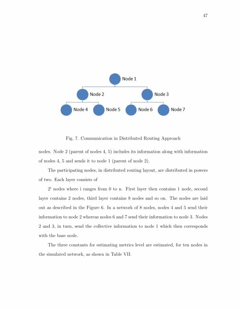
47

Fig. 7. Communication in Distributed Routing Approach

nodes. Node 2 (parent of nodes 4, 5) includes its information along with information

of nodes 4, 5 and sends it to node 1 (parent of node 2).

The participating nodes, in distributed routing layout, are distributed in powers

of two. Each layer consists of

2i nodes where i ranges from 0 to n. First layer then contains 1 node, second

layer contains 2 nodes, third layer contains 8 nodes and so on. The nodes are laid

out as described in the Figure 6. In a network of 8 nodes, nodes 4 and 5 send their

information to node 2 whereas nodes 6 and 7 send their information to node 3. Nodes

2 and 3, in turn, send the collective information to node 1 which then corresponds

with the base node.

The three constants for estimating metrics level are estimated, for ten nodes in

the simulated network, as shown in Table VII.

48

Table VII. Node Number and Corresponding Constant Values

Node α1 α2 α3

1 0.2 0.4 0.4

2 0.5 0.2 0.3

3 0.3 0.3 0.4

4 0.4 0.1 0.5

5 0.5 0.5 0.0

6 0.1 0.2 0.7

7 0.6 0.2 0.2

8 0.3 0.6 0.1

9 0.8 0.1 0.1

10 0.1 0.1 0.8

The variables used in the structure sensorNode, implemented in the simulation

are listed and described in Table VIII. The information displayed includes variable

type, variable name and the variable description.

5.2 Simulation Results

5.2.1 Time Taken by Participating Nodes to Send Information to the

Base Node

Time taken for a node to send information to the base node is imperative in eval-

uating the performance of the proposed Multi-Metric Adaptive Routing algorithm.

Processor time taken for the nodes to deliver the information to the base node is

estimated using clock() function in C language. Start time is noted at the sender

node and end time is noted at the receiver node. Difference of these times over

49

Table VIII. Variables Implemented and Corresponding Description

Variable Type Variable Name Variable Description

float packetAge Tracks packet duration in

the network

float nodeCEnergy Current energy level at the

node

float nodeIEnergy Initial energy level at the

node

float frequency Operating frequency of the

node

float metrics Metrics level to track the es-

timated metrics of the node

float α1 Used to calculate metrics

level

float α2 Used to calculate metrics

level

float α3 Used to calculate metrics

level

float alpha Absorption Coefficient

float distance Distance of the node to the

base node

int nodeDepth Depth of the node deployed

to the water surface

int hopCount Number of hops it takes for

the node to reach base sta-

tion

50

Table IX. Node Number, Time Taken to Transmit Packet to Base Node - 3 Nodes

Node ID Time Taken

Node 1 0.02 s

Node 2 0.01 s

Table X. Node Number, Time Taken to Transmit Packet to Base Node - 5 Nodes

Node ID Time Taken

Node 1 0.02 s

Node 2 0.02 s

Node 3 0.02 s

Node 4 0.02 s

CLOCKS PER SEC gives the processor time for that particular participant node to

transmit its information to the base node.

5.2.1.1 Time Calculation - Three Node Network Simulation

For a given minimum (3) number of nodes in a network, the time taken for

delivery is usually same. One simulation for 3 nodes result in the time observations

displayed in Table IX. The almost-ring approach implemented after the centralized

approach has taken 0.02 seconds.

5.2.1.2 Time Calculation - Five Node Network Simulation

Another instance of simulation (5 nodes - 0, 1, 2, 3, 4) reveals the time observa-

tions displayed in Table X. Here, it can be noted that all nodes take 0.02 seconds to

propagate information. The almost-ring approach implemented after the centralized

approach has taken 0.02 seconds.

51

Table XI. Node Number, Time Taken to Transmit Packet to Base Node - 15 Nodes

Node ID Time Taken

Node 1 0.04

Node 2 0.03

Node 3 0.05

Node 4 0.03

Node 5 0.05

Node 6 0.03

Node 7 0.03

Node 8 0.03

Node 9 0.05

Node 10 0.05

Node 11 0.03

Node 12 0.03

Node 13 0.03

Node 14 0.03

5.2.1.3 Time Calculation - Fifteen Node Network Simulation

A third instance of simulation with 15 nodes reveal interesting observations in

Table XI. Considerable change in the duration time for delivery can be observed in

the values above. The almost-ring approach after the centralized approach, in this

case, has taken 0.06 seconds.

52

Table XII. Node Number, Time Taken to Transmit Packet to Base Node - 50 Nodes

Nodes Value

24, 1, 26, 25, 3, 21, 20, 23,

12,

0.03

11, 7, 15, 13, 9, 18, 2, 28 0.04

30, 31, 32, 29, 33, 8, 17, 5,

35, 36, 37, 38, 34, 39, 40, 41,

42, 43, 44, 45, 48, 49, 46, 47,

27, 22, 19, 10, 16

0.05

4 0.06

14, 6 0.07

5.2.1.4 Time Calculation - Fifty Node Network Simulation

Significant difference in the time duration taken for packet transmission can be

observed in the fourth instance where 50 nodes are simulated in the network in Table

XII. Only some nodes are displayed that provide insightful information. It has taken

0.09 seconds to perform almost-ring communication in a network of 50 nodes.

53

Fig. 8. Time Observations (Seconds) for Centralized Routing Approach

5.3 Energy Analysis

Every node is powered initially with 100 units of power. For a packet of trans-

mission (assumed to be 1 byte), the energy consumed is calculated using the energy

model described in Section 3.5. Before a message is sent from sender to receiver, en-

ergy estimations are made and transmission is made only if there is sufficient energy

left in the participating node. The variable tracking a participating node’s current

energy is updated considering the initial energy at the node and energy consumed

for transmitting a packet. Apart from these calculations, α (absorption coefficient)

is estimated as described below

α = 0.11 ∗ f 2/(1 + f 2) + 44 ∗ f 2/(4100 + f 2) + 2.75/(104 ∗ f 2) + 0.03 (5.1)

where f - operating frequency of the participating node. Energy needed for

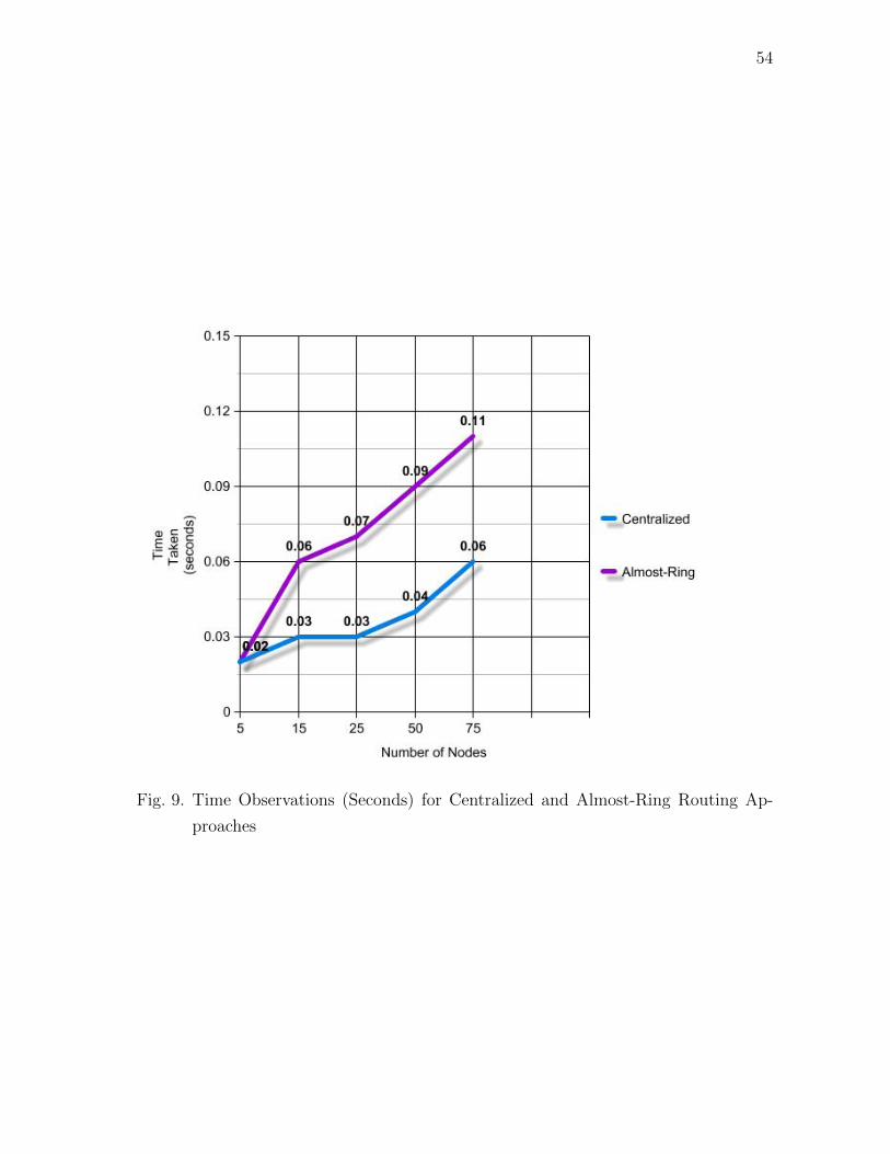
54

Fig. 9. Time Observations (Seconds) for Centralized and Almost-Ring Routing Ap-

proaches

55

Fig. 10. Time Observations (Seconds) for Centralized and Distributed Routing Ap-

proaches

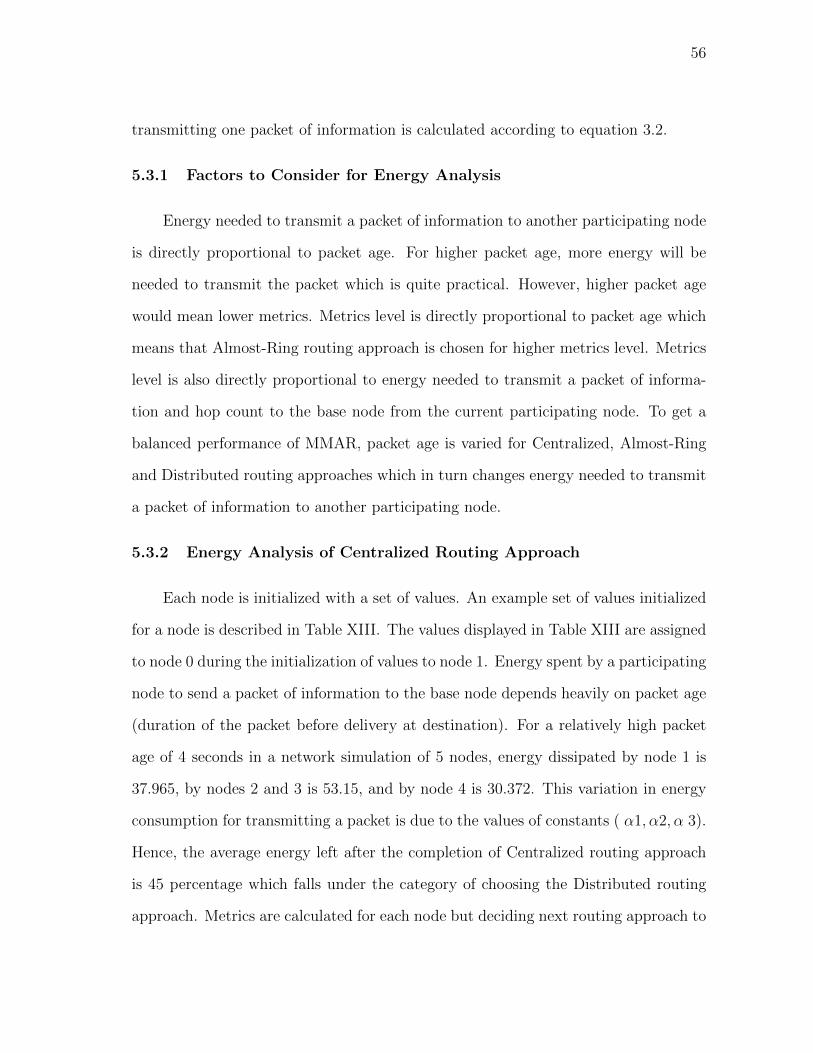
56

transmitting one packet of information is calculated according to equation 3.2.

5.3.1 Factors to Consider for Energy Analysis

Energy needed to transmit a packet of information to another participating node

is directly proportional to packet age. For higher packet age, more energy will be

needed to transmit the packet which is quite practical. However, higher packet age

would mean lower metrics. Metrics level is directly proportional to packet age which

means that Almost-Ring routing approach is chosen for higher metrics level. Metrics

level is also directly proportional to energy needed to transmit a packet of informa-

tion and hop count to the base node from the current participating node. To get a

balanced performance of MMAR, packet age is varied for Centralized, Almost-Ring

and Distributed routing approaches which in turn changes energy needed to transmit

a packet of information to another participating node.

5.3.2 Energy Analysis of Centralized Routing Approach

Each node is initialized with a set of values. An example set of values initialized

for a node is described in Table XIII. The values displayed in Table XIII are assigned

to node 0 during the initialization of values to node 1. Energy spent by a participating

node to send a packet of information to the base node depends heavily on packet age

(duration of the packet before delivery at destination). For a relatively high packet

age of 4 seconds in a network simulation of 5 nodes, energy dissipated by node 1 is

37.965, by nodes 2 and 3 is 53.15, and by node 4 is 30.372. This variation in energy

consumption for transmitting a packet is due to the values of constants ( α1, α2, α 3).

Hence, the average energy left after the completion of Centralized routing approach

is 45 percentage which falls under the category of choosing the Distributed routing

approach. Metrics are calculated for each node but deciding next routing approach to

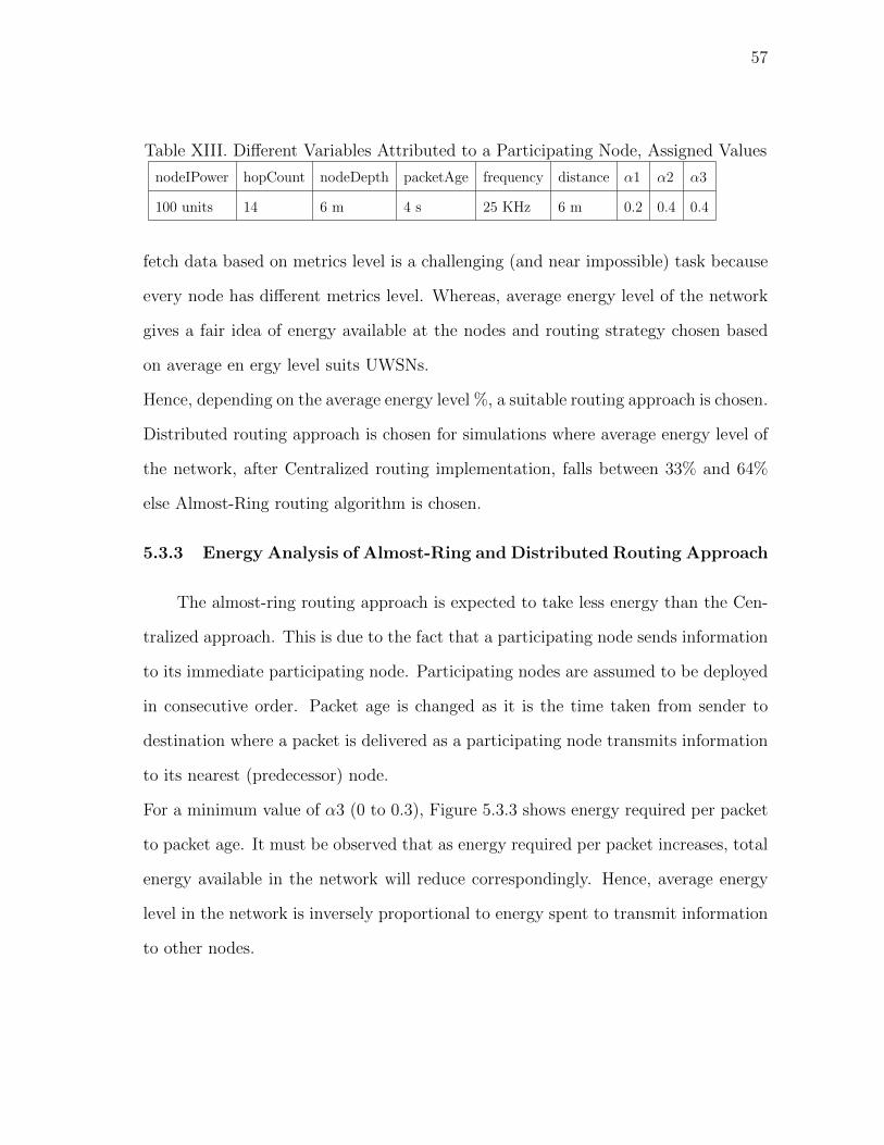
57

Table XIII. Different Variables Attributed to a Participating Node, Assigned Values

nodeIPower hopCount nodeDepth packetAge frequency distance α1 α2 α3

100 units 14 6 m 4 s 25 KHz 6 m 0.2 0.4 0.4

fetch data based on metrics level is a challenging (and near impossible) task because

every node has different metrics level. Whereas, average energy level of the network

gives a fair idea of energy available at the nodes and routing strategy chosen based

on average en ergy level suits UWSNs.

Hence, depending on the average energy level %, a suitable routing approach is chosen.

Distributed routing approach is chosen for simulations where average energy level of

the network, after Centralized routing implementation, falls between 33% and 64%

else Almost-Ring routing algorithm is chosen.

5.3.3 Energy Analysis of Almost-Ring and Distributed Routing Approach

The almost-ring routing approach is expected to take less energy than the Cen-

tralized approach. This is due to the fact that a participating node sends information

to its immediate participating node. Participating nodes are assumed to be deployed

in consecutive order. Packet age is changed as it is the time taken from sender to

destination where a packet is delivered as a participating node transmits information

to its nearest (predecessor) node.

For a minimum value of α3 (0 to 0.3), Figure 5.3.3 shows energy required per packet

to packet age. It must be observed that as energy required per packet increases, total

energy available in the network will reduce correspondingly. Hence, average energy

level in the network is inversely proportional to energy spent to transmit information

to other nodes.

58

Fig. 11. Relation of Packet Age to Energy Required Per Packet

5.4 Comparison to Other UWSN Routing Algorithms

Depth-Based Routing [3] relies on only one metric, namely, depth of the node

deployed. MMAR bases its decision considering several factors like packet age, hop

count and distance between nodes. After estimating the energy required for trans-

mitting information, the average energy level of the network is estimated. Then, a

routing strategy will be adapted based on the average energy level of the network

over all.

59

Table XIV. Comparison of Different UWSN Routing Algorithms

Algorithm Delivery Ratio Energy Consumption Event Synchronization Processing Multiple-Metrics

MMAR N/A Medium Logical Clock Linear Yes

DBR [3] High High No Medium No

VBF [8] Medium Medium No Medium No

HH-VBF [25] High Medium No Medium No

Table XV. Percentage of Energy Consumed by Nodes in Centralized Routing Ap-

proach

Node Number % Energy Consumed for

Sending Data

Packet Age - 1 % Energy Consumed for

Sending Data

Packet Age - 2

Node 1 22.78 2 53.15 6

Node 2 37.96 2 68.33 6

Node 3 37.96 2 68.33 6

Node 4 15.18 2 45.55 6

The effect of packet age on energy consumed in Almost-Ring routing approach

to send data is presented graphically in Figure 12.

Significant amount of energy is consumed in Centralized routing approach to

transmit information from participating nodes to the base node. On the other hand,

participating nodes consume relatively less energy for transmitting information to

Table XVI. Percentage of Energy Consumed by Nodes - Almost-Ring Routing Ap-

proach

Node Number % Energy Consumed for

Sending Data

Packet Age - 1 % Energy Consumed for

Sending Data

Packet Age - 2

Node 1 3.79 0.5 6.83 0.9

Node 2 3.79 0.5 6.83 0.9

Node 3 3.79 0.5 6.83 0.9

Node 4 3.79 0.5 6.83 0.9

60

Fig. 12. Increase in Energy Consumption with Packet Age

Table XVII. Dependence of Performance of Routing Approaches on Factors Involved

Routing Approach Packet Age Node Density

HH-VBF [25] No Yes

VBF [8] No Yes

MMAR Yes No

61

the base node using Distributed and Almost-Ring routing approaches. Percentage of

energy spent by participating nodes in the three routing approaches is tabulated in

Table XV, XVI. Node density affects performance in [25]. Even though more paths

are available for data delivery, more energy overhead is involved. MMAR sees no such

increase in energy with increase in node density. Instead, more energy per packet of

information is required if packet age increases. Also, it must be noted that MMAR

does not consider node mobility in its implementation. Table XVII lists the relation

between performance of routing approaches to the factors, such as packet age and

node density, involved. Time taken for delivery in Centralized routing approach is

better than in Almost- Ring and Distributed routing approaches but the amount of

energy consumed is vice-versa.

5.4.1 MMAR Performance Comparison with DBR and VBF Protocols

The performance of MMAR is compared with DBR protocol [3] and VBF protocol

[8]. Depth-Based Routing (DBR) protocol assumes geographical location of the nodes

similar to MMAR protocol. Sink-sink communication is not addressed in DBR similar

to how communication between base nodes is not addressed in MMAR. Nodes in

DBR send information to sinks in a greedy approach.Vector-Based Forwarding (VBF)

protocol uses source coordinates to calculate the position of current receiving node.

In DBR protocol, Priority Q and Packet History Buffer are used at each node.

Priority Q is used to decrease the number of forwarding nodes. Packet History Buffer

helps node decide not to send packets redundantly. MMAR does not use additional

buffers such as Priority Q and Packet History Buffer. While this saves communication

overhead at MMAR, it is a disadvantage that a history buffer is not implemented

in MMAR. Packet redelivery mechanism is available in VBF and DBR but not in

MMAR. Though it is advantageous to have packet redelivery mechanism, it can lead

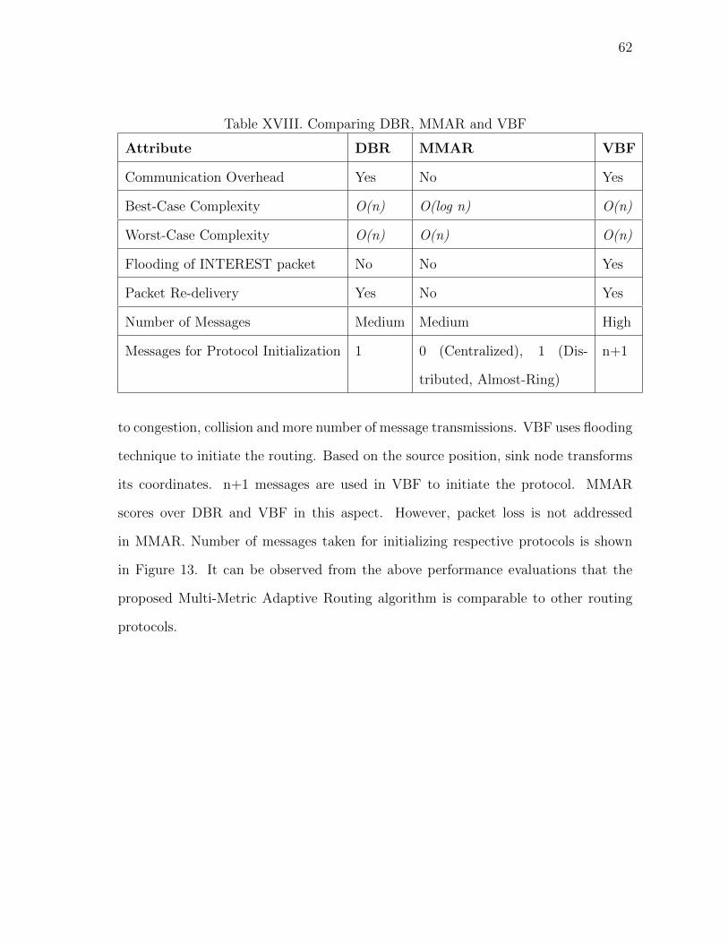
62

Table XVIII. Comparing DBR, MMAR and VBF

Attribute DBR MMAR VBF

Communication Overhead Yes No Yes

Best-Case Complexity O(n) O(log n) O(n)

Worst-Case Complexity O(n) O(n) O(n)

Flooding of INTEREST packet No No Yes

Packet Re-delivery Yes No Yes

Number of Messages Medium Medium High

Messages for Protocol Initialization 1 0 (Centralized), 1 (Dis-

tributed, Almost-Ring)

n+1

to congestion, collision and more number of message transmissions. VBF uses flooding

technique to initiate the routing. Based on the source position, sink node transforms

its coordinates. n+1 messages are used in VBF to initiate the protocol. MMAR

scores over DBR and VBF in this aspect. However, packet loss is not addressed

in MMAR. Number of messages taken for initializing respective protocols is shown

in Figure 13. It can be observed from the above performance evaluations that the

proposed Multi-Metric Adaptive Routing algorithm is comparable to other routing

protocols.

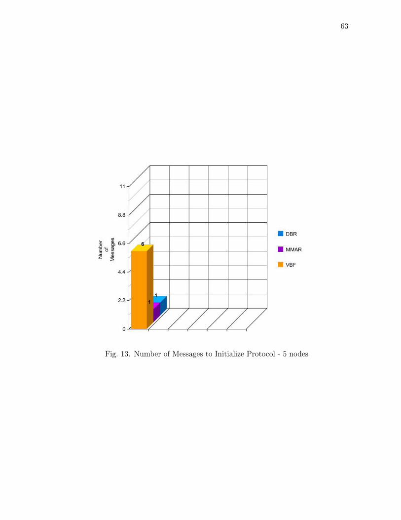
63

Fig. 13. Number of Messages to Initialize Protocol - 5 nodes

64

CHAPTER 6

FUTURE RESEARCH DIRECTIONS

Based on current research work to develop a Multi-Metric Adaptive Routing algo-

rithm for underwater wireless sensor networks, possible future research directions are

discussed in the following.

• Simulations in Different Environments

In C and MPI simulations, the issue of contention is already taken care of as

there is no competition for the resources. Ideally, messages must be transmitted

without collision and congestion. However, in real-world scenarios, synchroniza-

tion of messages is a major issue. Simulating Multi-Metric Routing algorithm in

multiple environments offers a new perspective on its performance in real-world

scenarios. Moreover, conclusive comparisons can be made with other routing

algorithms.

• Power Resources

Base node is assumed to be powered continuously in current implementation of

MMAR. However, in real-world applications, it may not be feasible to remotely

power nodes deployed on water surface. Moreover, base nodes need not be

floating on water surface as they can be underwater as well. Powering nodes

in such a scenario is extremely challenging as wired connections may not be an

ideal solution to energize nodes in underwater environments. Another reason

to ponder over this is that solar energy might not be applicable in UWSNs as

little sunlight reaches deep water consistently.

65

• Time Synchronization

Current implementation of MMAR does not look at synchronizing messages

considering the delays and disruptions in the underwater environment. Despite

the fact that an event synchronization mechanism is implemented using Lam-

port’s logical clock, it must be observed that time synchronization is different

from event synchronization. A robust UWSN might be undesirable without

time synchronization mechanism.

• Network Reconfiguration

MMAR works well until a node is compromised or dies. When the nodes are

not in expected topology as described in Section 3.3, the receiving participating

node waits endlessly hoping for the sender to transmit information which never

happens. This deadlock situation must be solved using a network recovery

algorithm.

• Security

The security of an UWSN has not been addressed in this thesis. Securing

communication in underwater environments is definite future research direction.

Currently, lightweight mechanisms for securing communication in WSNs such

as TinyPBC [37] are in place. However, a lightweight security scheme must be

developed that considers the low-energy necessities and realities of an UWSN.

Further research can be focused on addressing situations when a base node or

a participating node is under attack from an intruder.

• Base node selection

Base node selection can also be explored further. Floating node(s) need not be

base node(s) by default. Nodes deployed in the water can be base nodes as well.

They can be selected based on the ratio of the energy currently available to the

66

energy initially available. Another approach to select the base node is to assign

the node in the network with highest metrics level as the base node.

• Compatibility with Heterogeneous Networks

At some point of time, information transmitted to the base node by partici-

pating nodes must be sent to a data center. Developing suitable technology

to update database wirelessly using Internet is a viable option. However, the

economics of building such a technology must be thoroughly researched before

venturing in. Apart from the ability to connect to the world via the Internet,

feasible technology must be in place to interact with other ocean monitoring sys-

tems such as satellite imagery and buoy monitoring for effective and conclusive

results.

• Cluster-head Selection

Clusters can be formed by grouping nodes together. These clusters can choose

a cluster-head based on defined metrics. Without burdening a single node with

the responsibilities of a cluster-head, the functionalities of a cluster-head can

be shared with other nodes by choosing another node as cluster-head after

determined time period. Ultimately, all cluster-heads report to the base node.

Adaptive cluster-head selection for terrestrial wireless sensor networks has been

discussed in [38].

• Node Mobility

Our research does not consider node mobility in to account while developing the

routing strategy. Mobi-Sync research estimates velocity of nodes in underwater

environments [2]. This research can be used in improving the Multi-Metric

Adaptive Routing algorithm. Research in node mobility also extends scope for

further research in message and time synchronization that assists in addressing

67

congestion control in underwater environment.

• Localization

Localization is more challenging in UWSNs compared to terrestrial WSNs con-

sidering the lack of resources to re-energize deployed nodes. Finding the position

of deployed nodes in real-time is a major issue hindering routing for location-

based approaches. Every issue must be addressed within the bounds of efficient

hardware and software.

• Data aggregation

Data aggregation definitely can save energy and result in a longer life time pe-

riods for the network as a whole. Data aggregation is another definite future

research direction for building a robust UWSN with a comprehensive routing

strategy. More conclusive results can be obtained if simulations can be per-

formed using the NS-2 or OMNET++ simulators.

68

CHAPTER 7

CONCLUSION

A novel routing algorithm for underwater wireless sensor networks has been proposed.

This Multi-Metric Adaptive Routing algorithm considers multiple metrics such as

depth of the node deployed, packet age, energy level at the node, average energy

level in the network and hop count of a node to the base node. The routing strategy

is dynamic depending on the mentioned metrics. The possible routing techniques

are centralized, distributed and almost-ring approaches. The time taken for message

transmission for network simulation ranging from 5 to 50 nodes has been observed and

reported. Energy analysis of the participating nodes has also been performed. Al-

gorithmic complexities of Centralized, Almost-Ring, Distributed routing approaches

and Mult-Metric Adaptive Routing algorithm have been presented. The overall com-

plexity of MMAR is reported as O(log n) + O(n) and O(n) for large values of n.

Further, communication and space complexities of the proposed routing algorithm

have been detailed. Number of messages taken is O(n) for Centralized, Distributed

and Almost-Ring routing approaches. In the worst case scenario, MMAR takes O(3n

- 3) messages and O(n - 1) messages. Event synchronization is implemented using

Lamport’s logical clock. MMAR takes advantage of its implementation in C language

and MPI and exploits the extension of logical clock support in distributed systems.

A comparison of MMAR with DBR and VBF protocols has been performed.

Additionally, a case study has been presented to forecast red tides and results are

detailed. Two approaches to forecast red tides using UWSNs are proposed in the

case study. The first approach is using TinyDB and TOSSIM simulations which have

69

the native support of TinyOS, widely used software for sensor nodes, but cannot sim-

ulate more than one value at a time. The second approach to forecast red tides is by

using C language and Message Passing Interface. The second approach can estimate

multiple values per node but C language is not supported natively by TinyOS.

70

REFERENCES

[1] U. Lee, P. Wang, Y. Noh, L. F. M. Vieira, M. Gerla, and J.-H. Cui, “Pressure

routing for underwater sensor networks,” in Proceedings of the 29th conference on

Information communications, INFOCOM’10, (Piscataway, NJ, USA), pp. 1676–

1684, IEEE Press, 2010.

[2] J. Liu, R. Z. Zhou, J. P. Zheng, and J.-H. Cui, “Mobi-sync: Efficient time

synchronization for mobile underwater sensor networks,” in GLOBECOM, pp. 1–

5, Proceedings of the Global Communications Conference, 2010. GLOBECOM

2010, 6-10 December 2010, Miami, Florida, USA, 2010.

[3] H. Yan, Z. J. Shi, and J.-H. Cui, “Dbr: depth-based routing for underwater

sensor networks,” in Proceedings of the 7th international IFIP-TC6 networking

conference on AdHoc and sensor networks, wireless networks, next generation

internet, NETWORKING’08, (Berlin, Heidelberg), pp. 72–86, Springer-Verlag,

2008.

[4] “Dynamically reconfigurable underwater marine wireless sensor networks,” May

2011. http://subseaworldnews.com/2011/05/05/beenish-ayaz-begins-research-

project-dynamically-reconfigurable-underwater-wireless-sensor-networking-at-

nsri-uk/.

[5] “Project neptune,” NEPTUNE, December 2010.

http://www.neptunecanada.ca/.

[6] M. Ayaz and A. Abdullah, “Underwater wireless sensor networks: routing issues

and future challenges,” in Proceedings of the 7th International Conference on

71

Advances in Mobile Computing and Multimedia, MoMM ’09, (New York, NY,

USA), pp. 370–375, ACM, 2009.

[7] L. Lanbo, Z. Shengli, and C. Jun-Hong, “Prospects and problems of wireless

communication for underwater sensor networks,” Wirel. Commun. Mob. Com-

put., vol. 8, pp. 977–994, October 2008.

[8] P. Xie, J. hong Cui, and L. Lao, “Vbf: Vector-based forwarding protocol for

underwater sensor networks,” in In Proc. of IFIP Networking, pp. 1216–1221,

2005.

[9] S. Tilak, N. B. Abu-Ghazaleh, and W. Heinzelman, “Infrastructure tradeoffs

for sensor networks,” in Proceedings of the 1st ACM international workshop on

Wireless sensor networks and applications, WSNA ’02, (New York, NY, USA),

pp. 49–58, ACM, 2002.

[10] K. Ovaliadis, N. Savage, and V. Kanakaris, “Energy efficiency in underwater sen-

sor networks: a research review,” Journal of Engineering Science and Technology

Review, vol. 3, no. 1, pp. 151–156, 2010.

[11] R. Gitzendanner, F. Puglia, C. Martin, D. Carmen, E. Jones, and S. Eaves,

“High power and high energy lithium-ion batteries for under-water applications,”

Journal of Power Sources, vol. 136, no. 2, pp. 416 – 418, 2004. Selected papers

presented at the International Power Sources Symposium.

[12] J. hong Cui, J. Kong, M. Gerla, and S. Zhou, “Challenges: Building scalable

mobile underwater wireless sensor networks for aquatic applications,” IEEE Net-

work, Special Issue on Wireless Sensor Networking, vol. 20, p. 2006, 2006.

72

[13] Kim, H. Gyoon, S. G. Lee, C. K. Lee, and W. A. Lim, “Korean red tide moni-

toring and prediction system.”

[14] A. Salhieh, J. Weinmann, M. Kochhal, and L. Schwiebert, “Power efficient

topologies for wireless sensor networks,” in In International Conference on Par-

allel Processing, pp. 156–163, 2001.

[15] S. yun Kim, O. Guzide, and S. Cook, “Towards an optimal network topology in

wireless sensor networks,” in SUJUR, vol. 1, 2009.

[16] L. Liu, “A qos-based topology control algorithm for underwater wireless sensor

networks,” in International Journal of Distributed Sensor Networks, no. 642053,

2010.

[17] L. Liu, “A topology recovery algorithm of underwater wireless sensor networks,”

in Communication Technology (ICCT), 2010 12th IEEE International Confer-

ence on, pp. 64 –67, nov. 2010.

[18] J. P. Walters, Z. Liang, W. Shi, and V. Chaudhary, “Wireless sensor network

security: A survey, in book chapter of security,” in in Distributed, Grid, and

Pervasive Computing, Yang Xiao (Eds), pp. 0–849, CRC Press, 2007.

[19] Y. Cong, G. Yang, Z. Wei, and W. Zhou, “Security in underwater sensor net-

work,” Communications and Mobile Computing, International Conference on,

vol. 1, pp. 162–168, 2010.

[20] F. Salva-Garau and M. Stojanovic, “Multi-cluster protocol for ad hoc mobile

underwater acoustic networks,” in OCEANS 2003. Proceedings, vol. 1, pp. 91

–98 Vol.1, sept. 2003.

73

[21] M. C. Domingo and R. Prior, “Design and analysis of a gps-free routing protocol

for underwater wireless sensor networks in deep water,” in Proceedings of the

2007 International Conference on Sensor Technologies and Applications, SEN-

SORCOMM ’07, (Washington, DC, USA), pp. 215–220, IEEE Computer Society,

2007.

[22] S. Gopi, K. Govindan, D. Chander, U. B. Desai, and S. N. Merchant, “E-pulrp:

energy optimized path unaware layered routing protocol for underwater sensor

networks,” Trans. Wireless. Comm., vol. 9, pp. 3391–3401, November 2010.

[23] T. Hu and Y. Fei, “An adaptive and energy-efficient routing protocol based

on machine learning for underwater delay tolerant networks,” Modeling, Analy-

sis, and Simulation of Computer Systems, International Symposium on, vol. 0,

pp. 381–384, 2010.

[24] H. Nam and S. An, “Energy-efficient routing protocol in underwater acoustic

sensor networks,” 2010.

[25] N. Nicolaou, A. See, J. hong Cui, and D. Maggiorini, “Improving the robustness

of location-based routing for underwater sensor networks,” in In MTS/IEEE

OCEANS conference, 2007.

[26] X. Che, I. Wells, P. Kear, G. Dickers, X. Gong, and M. Rhodes, “A static multi-

hop underwater wireless sensor network using rf electromagnetic communica-

tions,” in Distributed Computing Systems Workshops, 2009. ICDCS Workshops

’09. 29th IEEE International Conference on, pp. 460 –463, june 2009.

[27] S. Park, B. Jo, and D.-S. Han, “An efficient mac protocol for data collection in

underwater wireless sensor networks,” in Proceedings of the 28th IEEE conference

74

on Military communications, MILCOM’09, (Piscataway, NJ, USA), pp. 348–352,

IEEE Press, 2009.

[28] Z. Guo, G. Colombo, B. Wang, J.-H. Cui, D. Maggiorini, and G. Rossi, “Adaptive

routing in underwater delay/disruption tolerant sensor networks,” in Wireless

on Demand Network Systems and Services, 2008. WONS 2008. Fifth Annual

Conference on, pp. 31 –39, jan. 2008.

[29] E. M. Sozer, M. Stojanovic, and J. G. Proakis, “Underwater acoustic networks,”

vol. 25, pp. 72 –83, IEEE Journal of Oceanic Engineering, Jan 2000.

[30] W. R. Heinzelman, A. Chandrakasan, and H. Balakrishnan, “Energy-efficient

communication protocol for wireless microsensor networks,” in Proceedings of the

33rd Hawaii International Conference on System Sciences-Volume 8 - Volume 8,

HICSS ’00, (Washington, DC, USA), pp. 8020–, IEEE Computer Society, 2000.

[31] L. Lamport, “Ti clocks, and the ordering of events in a distributed system,”

Commun. ACM, vol. 21, pp. 558–565, July 1978.

[32] N. Stroppa, “Algorithms & complexity - introduction,” November 2006.

[33] W. W. Cheng, L. Hall, D. Goldgof, I. Soto, and C. Hu, “Automatic red tide

detection from modis satellite images,” in Systems, Man and Cybernetics, 2009.

SMC 2009. IEEE International Conference on, pp. 1864 –1868, oct. 2009.

[34] I. Lake and L. Funkquist, “Operational forecasts of algae blooms in the baltic

sea,” in US/EU-Baltic International Symposium, 2008 IEEE/OES, pp. 1 –6, may

2008.

[35] H. Nam and S. An, “Energy-efficient routing protocol in underwater acoustic sen-

sor networks,” in Proceedings of the 2008 IEEE/IFIP International Conference

75

on Embedded and Ubiquitous Computing - Volume 02, EUC ’08, (Washington,

DC, USA), pp. 663–669, IEEE Computer Society, 2008.

[36] M. Snir, S. Otto, S. Huss-Lederman, D. Walker, and J. Dongarra, MPI-The

Complete Reference, Volume 1: The MPI Core. Cambridge, MA, USA: MIT

Press, 2nd. (revised) ed., 1998.

[37] L. Oliveira, M. Scott, J. Lopez, and R. Dahab, “Tinypbc: Pairings for authen-

ticated identity-based non-interactive key distribution in sensor networks,” in

Networked Sensing Systems, 2008. INSS 2008. 5th International Conference on,

pp. 173 –180, june 2008.

[38] C.-S. Nam, H.-J. Jeong, and D.-R. Shin, “The adaptive cluster head selection

in wireless sensor networks,” in Proceedings of the 2008 IEEE International

Workshop on Semantic Computing and Applications, (Washington, DC, USA),

pp. 147–149, IEEE Computer Society, 2008.

76

APPENDIX A

FORECASTING RED TIDES USING TINYDB AND TOSSIM

The discussed contributing factors are the primary reason for causing red tides in wa-

ter. Contributing factors that are considered for this research include temperature,

salinity, turbidity, dissolved oxygen, pH, sunlight, nitrate, chlorophyll-a and wind.

Python scripts are written to simulate contributing factors. Cygwin, Windows XP,

TinyOS, TOSSIM and TinyDB are primarily used for this simulation. This tutorial

explains how to forecast red tides using underwater wireless sensor networks using

TOSSIM, TinyDB environments by loading TinyDB application, simulation interface

and executing scripts in that order. This tutorial does not explain extracting infor-

mation after querying using TinyDB graphical user interface. The following steps are

implemented to simulate the network that forecasts red tides.

Step 1

Copy all the script files to the folder ’$TOSROOT/tools/java/net/tinyos/sim’

Step 2

Copy the Java file to the folder ’$TOSROOT/tools/java/net/tinyos/tinydb’ that

queries TinyDB and adds the out-coming result to a vector.

The files need to be copied only once. Then, these steps need to be executed (in

Cygwin window)

1. TinyDBApp

Execute these commands in a Cygwin window.

cd $TOSROOT/apps/TinyDBApps

77

export DBG=usr1

build/pc/main.exe 31

The above commands open the simulation interface.

2. TinyDBMain

Execute these commands in a second Cygwin window.

cd ’\$TOSROOT/tools/java’

java net.tinyos.tinydb.TinyDBMain -sim

The above comamnds execute TinyDB application.

3. Execute Scripts

Tython environment is opened to execute scripts.

cd $TOSROOT/tools/java/net/tinyos/sim

java -jar simdriver.jar

(in Tython environment) from simcore import *

execfile("oxygen-simulation.py")

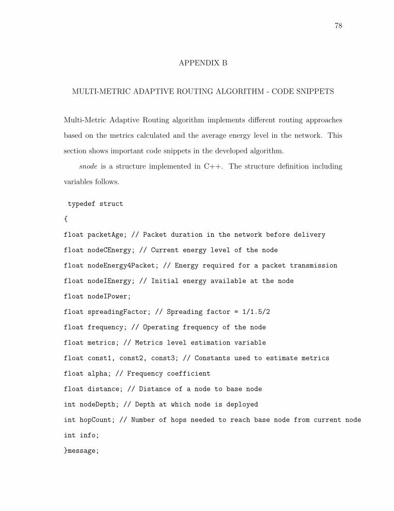
78

APPENDIX B

MULTI-METRIC ADAPTIVE ROUTING ALGORITHM - CODE SNIPPETS

Multi-Metric Adaptive Routing algorithm implements different routing approaches

based on the metrics calculated and the average energy level in the network. This

section shows important code snippets in the developed algorithm.

snode is a structure implemented in C++. The structure definition including

variables follows.

typedef struct

{

float packetAge; // Packet duration in the network before delivery

float nodeCEnergy; // Current energy level of the node

float nodeEnergy4Packet; // Energy required for a packet transmission

float nodeIEnergy; // Initial energy available at the node

float nodeIPower;

float spreadingFactor; // Spreading factor = 1/1.5/2

float frequency; // Operating frequency of the node

float metrics; // Metrics level estimation variable

float const1, const2, const3; // Constants used to estimate metrics

float alpha; // Frequency coefficient

float distance; // Distance of a node to base node

int nodeDepth; // Depth at which node is deployed

int hopCount; // Number of hops needed to reach base node from current node

int info;

}message;

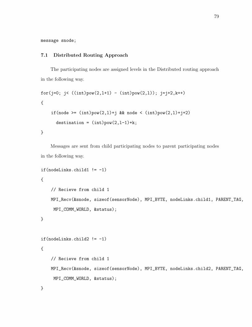
79

message snode;

7.1 Distributed Routing Approach

The participating nodes are assigned levels in the Distributed routing approach

in the following way.

for(j=0; j< ((int)pow(2,l+1) - (int)pow(2,l)); j=j+2,k++)

{

if(node >= (int)pow(2,l)+j && node < (int)pow(2,l)+j+2)

destination = (int)pow(2,l-1)+k;

}

Messages are sent from child participating nodes to parent participating nodes

in the following way.

if(nodeLinks.child1 != -1)

{

// Recieve from child 1

MPI_Recv(&snode, sizeof(sensorNode), MPI_BYTE, nodeLinks.child1, PARENT_TAG,

MPI_COMM_WORLD, &status);

}

if(nodeLinks.child2 != -1)

{

// Recieve from child 1

MPI_Recv(&snode, sizeof(sensorNode), MPI_BYTE, nodeLinks.child2, PARENT_TAG,

MPI_COMM_WORLD, &status);

}

80

where PARENT TAG is 222.

7.2 Almost-Ring Routing Approach

The start of Almost-Ring routing approach is signalled by the base node to the

last node in the simulation.

if(node == 0)

{ // Send Signal to Last Node to begin Ring Communication

MPI_Send(&snode, sizeof(message), MPI_BYTE, size-1, RING_SIGNAL_TAG,

MPI_COMM_WORLD, &status);

}

if(node == (size-1))

{ // Get Signal from Node 0 to begin Ring Communication

MPI_Recv(&snode, sizeof(message), MPI_BYTE, 0, RING_SIGNAL_TAG,

MPI_COMM_WORLD, &status);

}

where RING SIGNAL TAG is 666.

7.3 Energy and Metrics Calculations

snode.alpha = 0.11*f*f/(1 + f*f) + 44*f*f/(4100 + f*f) + 2.75/(pow(10,4)*f*f)

+ 0.03; // Thorp’s Expression

snode.nodeEnergy4Packet = snode.nodeIPower*snode.packetAge*

(pow(snode.distance,snode.spreadingFactor))*(pow(snode.alpha,snode.distance));

snode.metrics = snode.const1*snode.packetAge + snode.const2*snode.nodeEnergy4Packet

+ snode.const3*snode.hopCount;