musical metacreation: modeling polyphony with neural networks
TRANSCRIPT

Musical Metacreation: Modeling Polyphony
with Neural NetworksFRANCISCO ELÍAS MONTAÑEZ
DIVISION OF SCIENCE AND MATHEMATICS
UNIVERSITY OF MINNESOTA, MORRIS
MORRIS, MINNESOTA, USA
NOVEMBER 17, 2018

Outline
I. Background
II. JamBot
III. Results
IV. Conclusion
2

Outline
I. Background
• Texture
• What is a neural network?
II. JamBot
III. Results
IV. Conclusion
3

Texture
• Describes musical layers in terms of
number and purpose
• Monophonic
• Polyphonic
4

Monophonic vs Polyphonic
Polyphonic
• Multiple layers
• More than one note at a time
Monophonic
• Single layer
• One note at a time
5

MIDI via Piano Roll
• Musical Instrument Digital Interface
• No sound
• Carries events that represent note
information
Event: Note ON
Event: Note OFF
6
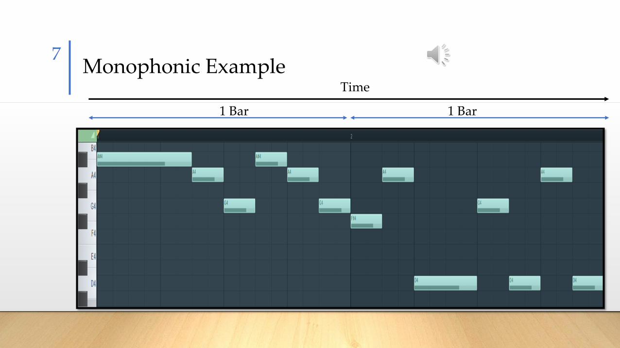
Monophonic ExampleTime
7
1 Bar 1 Bar

Polyphonic Example8
Time
1 Bar 1 Bar

Difficulty of Modeling Polyphony
• Music is sequential
• Maintaining coherence
• Coincidences of notes
9

Outline
I. Background
• Texture
• What is a neural network?
II. JamBot
III. Results
IV. Conclusion
10

Overview
• Framework modeled loosely after
the human brain
• Designed to recognize patterns in
data
• Learn to perform tasks by
considering examples, generally
without being programmed
11

Network Structure
• Input layer
• Hidden layer(s)
• Output layer
Input layer
Hidden layer
Output layer
12

Node Structure
• Inputs X1, X2, X3
• Weights W1, W2, W3
• Activation function f(x)
• Output Y
13

Training
• Process of improving networks
ability of making predictions
• Supervised – each dataset sample
has an expected output
• Purpose is to adjust weights so the
predicted output is reasonably close
to expected output
14

Training
• Dataset is split into training and
testing sets
• Weights are initialized randomly
• Training set is run through the
network
15
Training
• Loss function determines how close
predicted output is to expected
output
• Lower value = higher accuracy
• Higher value = lower accuracy
• We want to minimize loss function
16

Training
• Gradient – direction and size of each
loss function
• Backpropagation calculates
gradients
• Gradient descent uses gradients to
update weights accordingly
17

Training
• Process is repeated until predicted
output is reasonably close to the
expected output
• Testing set is used to evaluate the
network
18

Training Difficulties
• Vanishing gradient – size of
gradients decrease exponentially as
they are distributed back through
network layers
• Network is unable to learn or learns
extremely slow
19

Training Difficulties
• Exploding gradients – size of
gradients increases exponentially
causing an unstable network
• Weights are unable to be updated
20

Training Difficulties
• Overfitting – network learns training
data too well
• Network performs well on training
set but poorly on testing set
• Unable to generalize on new data
21

Outline
I. Background
II. JamBot
III. Results
IV. Conclusion
22

Remember
• Music is sequential
• Must know what has been played to
determine what could be played
next
23
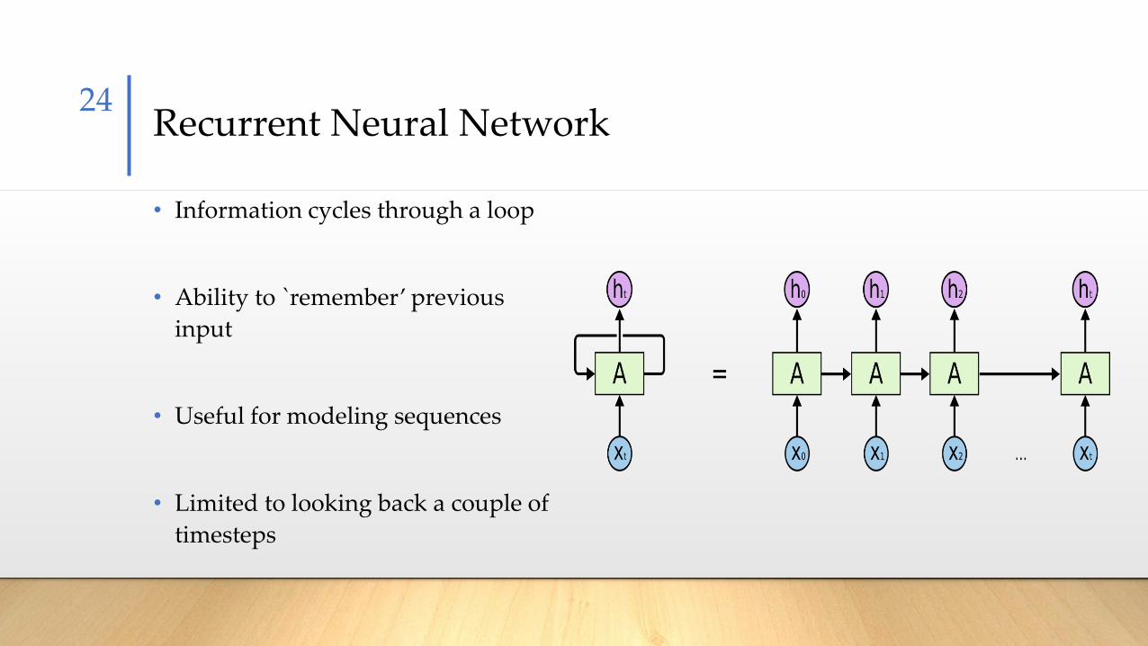
Recurrent Neural Network
• Information cycles through a loop
• Ability to `remember’ previous
input
• Useful for modeling sequences
• Limited to looking back a couple of
timesteps
24

LSTM Network
• Introduces memory cells with gating
architecture
• Gates decide whether cells should
keep or forget previous states in
each loop
• Allow modeling of long term
sequences
25

JamBotOverview
• Composed of Chord LSTM and
Polyphony LSTM
• Chord LSTM outputs probabilities of
every chord to be played in next bar
• Polyphonic LSTM outputs
probabilities of every note to be
played in next timestep
26

Outline
I. Background
II. JamBot
• Training Data
• Chord LSTM
• Polyphonic LSTM
III. Results
IV. Conclusion
27

Training Data
• Subset of Lakh MIDI dataset
consisting of 86,000 MIDI files
• All MIDI data is in Major/relative
Minor scale
• Transposed to same key
Lakh MIDI Dataset Scales
28

Outline
I. Background
II. JamBot
• Training Data
• Chord LSTM
• Polyphonic LSTM
III. Results
IV. Conclusion
29

Chord LSTM
• 3 most occurring notes in every bar
form a chord
• 50 most occurring chords replaced
with IDs
• Chord/ID pair stored in dictionary
• Encoded as vectors Xchord
30

Chord LSTM
• Embedding matrix Wembed used to
capture relationships between
chords
• Xchord · Wembed = Xembed
• Xembed used as input
10-Dimensional Chord Embedding Xembed
.
.
.
1.76-2.190.37
.
.
.
11
Chord ID
31

Chord LSTM32
• Goal is to learn meaningful
representation of chords
• Outputs vectors that contain
probabilities for all chords to be
played next
11
4
45
36
7
32
Chord IDs in Embedding Space
24
12
26
41
9
15
18
17

Prediction
• Feed seed of variable length into
network
• Next chord predicted by sampling
output probability with hyper-
parameter temperature
33

Prediction
• Temperature = 0
• No variation in prediction
34
• Temperature = 1
• Lots of variation in prediction

Outline
I. Background
II. JamBot
• Training Data
• Chord LSTM
• Polyphonic LSTM
III. Results
IV. Conclusion
35

Polyphonic LSTM
• Piano roll data is extracted from
dataset
36

Polyphonic LSTM
• Notes played at each timestep
represented as vectors
• Entry = 1 if note is played
• Entry = 0 if not is not played
No
tes
time
37

Polyphonic LSTM
• Piano roll vector
• Embedded chord of next timestep
• Embedded chord which follows
chord of next timestep
• Binary counter
38
xtpoly =

Polyphonic LSTM
• Input vectors fed to network
• Output of LSTM at time t = ytpoly
• Outputs vector with same number of entries as there are notes
• Every entry is probability of the corresponding note to be played at next time step conditioned on all inputs of the timesteps before
39

Prediction
• Feed seed consisting of piano roll
and corresponding chords
• Notes which are played at next time
step are sampled from output vector
ytpoly
• Notes are sampled independently
40

Outline
I. Background
II. JamBot
III. Results
IV. Conclusion
41

Results
• JamBot Generation - Song 2 , Tempo
140 BPM, Instrument Electric Guitar
(Jazz)
• JamBot Generation - Song 3, Tempo
160 BPM, Instrument Bright Acoustic
Piano
• JamBot Generation - Song 4, Tempo
100 BPM, Instrument Orchestral Harp
42

Outline
I. Background
II. JamBot
III. Results
IV. Conclusion
43

Conclusion
• Generated music has long term structure
• Coherence is present and music is pleasing
• Learned meaningful embeddings where related chords are closer together in embedding space
• Missing emotional build
44

Acknowledgements
Thank you for your time!
Thank you to my advisor Elena Machkasova for her
guidance and feedback.
45

Questions?
46

References
• G. Brunner, Y. Wang, R. Wattenhofer and J. Wiesendanger, "JamBot: Music Theory Aware
Chord Based Generation of Polyphonic Music with LSTMs," 2017 IEEE 29th International
Conference on Tools with Artificial Intelligence (ICTAI), Boston, MA, 2017, pp. 519-526.
• Philippe Pasquier, Arne Eigenfeldt, Oliver Bown, and Shlomo Dubnov. 2017. An Introduction
to Musical Metacreation. Comput. Entertain. 14, 2, Article 2 (January 2017), 14 pages. DOI:
https://doi.org/10.1145/2930672
• https://www.youtube.com/channel/UCQbE9vfbYycK4DZpHoZKcSw
47

Image References
• Humphreys, Paul. “4. Conceptual Emergence and Neural Networks.” The Brains Blog, 16 Nov.
2017, philosophyofbrains.com/2017/11/16/4-conceptual-emergence-neural-networks.aspx.
• “Deep Neural Network's Precision for Image Recognition, Float or Double?” Stack Overflow,
stackoverflow.com/questions/40537503/deep-neural-networks-precision-for-image-recognition-
float-or-double.
• “Microbiome Summer School 2017.” Microbiome Summer School 2017 by aldro61,
aldro61.github.io/microbiome-summer-school-2017/sections/basics/.
48

Image References
• Shanmugamani, Rajalingappaa. “Deep Learning for Computer Vision.” O'Reilly | Safari,
O'Reilly Media, Inc., www.oreilly.com/library/view/deep-learning-
for/9781788295628/a32bda93-3658-42ff-b369-834b9c7052e8.xhtml.
• Olah, Chris. “Understanding LSTM Networks.” Understanding LSTM Networks -- Colah's
Blog, colah.github.io/posts/2015-08-Understanding-LSTMs/.
49