MPRAMunich Personal RePEc Archive

Commodity Prices and MacroeconomicVariables in India: An Auto-RegressiveDistributed Lag (ARDL) Approach

Pratap Kumar Jena

North Orissa University

2015

Online at https://mpra.ub.uni-muenchen.de/73892/MPRA Paper No. 73892, posted 6 January 2017 12:50 UTC

1

Commodity Prices and Macroeconomic Variables in India: An Auto-Regressive

Distributed Lag (ARDL) Approach

Pratap Kumar Jena

Assistant Professor, Department of Economics, North Orissa University, Baripada,

Odisha- 757003, India;

Abstract: This paper examines the relationship between commodities index prices and

macroeconomic variables in India over the period of January 2001 to June 2012 using the time

series techniques of ARDL model and ECM model. The ARDL test suggests that there is long-

run cointegration between agriculture index price and macroeconomic variables, and also

between energy index price and macroeconomic variables. But, there is no long-run

cointegration between metal index price and macroeconomic variables. The results also indicate

that IIP and Exchange rate have positive and significant effects on the agricultural index price.

This implies that that IIP and Exchange rate are vital macroeconomic variables that influence the

agricultural index price in the study period. Similarly, the aggregate demand (i.e. IIP) is the

positive and significant effect on energy index price. This implies that that IIP is a vital

macroeconomic variable that influences the energy index price in the study period. But, there is

no such macroeconomic variable we found which have a significant effect on the metal index

price.

Keywords: Commodity Price, Macroeconomic, ARDL, ECM

JEL Classification: E31, E01 ,C51

1. Introduction:

In the 21st century, the volatility of commodity prices has taken attention of policy makers and

academic researchers to study on commodity markets in world-wide. The recent rose of

commodity prices since 2002 to mid of 2008 is exceptional in terms of a number of commodities

and duration. Commodities have multiple uses in day to day life and its demand is always greater

than the supply. Therefore, the recent rise in commodity prices is not only put a heavy burden on

developing and emerging economies like India and also it fuels inflation in the country. There

are arguments and debates to understand what are the causes and consequences of the recent rise

of commodity prices in India. In the debate and arguments, researchers have given more

importance to two factors, which are well connected. Firstly, they gave importance to

2

fundamental factors and secondly, they gave importance to the financialization of commodity

markets.

The recent raises of commodities prices are due to growing of world income and there is

no match between the supply of and demand for commodities (OECD-FAO, 2008). The second

fold of argument attributes to the recent rising of financialisation of commodity markets

(UNCTAD report, 2009). The strong and sustained increase in primary commodity prices from

2002 to 2008 was attended by the growing financial investors on commodity futures exchanges,

as investors use commodity as an alternative investment asset class. The investors are not

interested in individual commodity but they are interested in investing on group of commodities

like index investment. Since 2003 to mid-2008 there has been continuously increased the total

value of various commodity index-related investments estimated $15 billion to $200 billion

(CFTC staff report, 2008).

Commodity prices in the international market have dramatized trends; sometimes there

have continuous upward trends and sometimes downward trends. But, commodity prices started

rising in a different way since 2002 and it severely hit by the global financial crisis in the mid of

2008. It is observed that the prices of some commodities reached even historic high in nominal

and real terms in metals, minerals and crude oil. But, due to the crisis, commodity prices

experienced a sharp fall due to global economic uncertainties and financial shocks. It continued

to till the global economy recovered from the crisis in 2009. Thereafter, commodity prices

started upward trend during the first quarter of 2009 despite the continuation of the global

economic downturn.

Basically, agricultural and food commodity prices were severely heated by the financial

downturn and long-term declined nearly 50% in real prices than other commodities. Such price

declined led to low income and low economic growth of agricultural producers and developing

countries. Another reason for rising commodity prices is the Doha Round of WTO, they reduced

the agricultural support and trade barriers for the developed or high-income nations. It led to a

rising of commodity prices, income and welfare of the agricultural commodities exporting

countries (Aksoy & Beghin, 2005 and Anderson & Masters, 2009).

There are many common factors which influence commodity markets. The price

dynamics are differing across commodity groups. For example, the global economic recession

3

has not affected all sectors in the same way. Some sectors, such as sugar and coffee, are

benefited from increased demand, whereas others, such as cotton, has hit hard by the crisis.

Similarly, climatic shocks have also differed across agricultural commodity groups (UNCTAD,

2010).

Commodity prices in India were peaked before the mid of 2008 but became low during

the depth of the financial crisis. Before mid-2008, energy prices were more than double and it

became $144 per barrel. Similarly, metals prices were up 150 percent while agricultural prices

were 77 or higher (MCX Commodity Year Book, 2011). There was sharp fall of food, metals

and energy prices during the financial crisis in world-wide. But in the early of 2009, all

commodity prices came to the old track due to stimulus packages and policy actions by the

Indian government.

The vast public attention takes place on increase in commodity price volatility but and

growth of commodity index investment has gone unnoticed among them. Therefore, the present

study investigates to find out the possible macroeconomic factors that help the recent boom of

commodity prices in India. Therefore, this paper is organized into following sections. Section-2

deals with literature review. Sample size and data sources are reported in section-3. In section-4,

we have reported the methodology of the study. In section-5, we have reported the analysis of

estimated results. The last section-6 gives the conclusion of the study.

2. Literature Review

The high volatility of commodity prices in India gives pain to policy makers and researchers to

find out the reasons behind it. This leads to difficulty in predicting the commodity prices of

essential commodities. Among factors, the macroeconomic factors attract more to the policy

makers and researchers. As the macroeconomic factors play the major role in the change in

demand and supply. Different economists have suggested different macroeconomic factors

which affect commodity prices both in the short-run and in the long-run. Therefore, this paper

attempts to find out factors which affect commodity price in India. There are studies like;

Dornbusch (1985), Lescaroux (2009), Borensztein and Reinhart (1994), Chambers and Bailey

(1996), Labys and Maizels (1990), Frankel and Hardouvelis (1985), Christie-David, et al. (2000),

4

Kim et al. (2011), Nag and Goswami (2008), Kabia and Gil (2000), Kaufmann (2011), Palaskas

and Varangis (1991), Frankel (2006), Gilbert (1990), Anderson and et al. (2003) , Barnhart

(1989), Cai, Cheung and Wong (2001), Erb and Harvey (2006) and etc, which show the

relationship between macroeconomic factors and commodity prices,

Durnbusch (1984) shows the effects of real exchange rate on commodity price. Lescaroux

(2009) examined the excess-comovement of commodity prices- a special reference to how

fundamental factors are playing a major role in short-run dynamics. His framework was unable

to explain the marked and sustained weakness in commodity prices during the 1980s and 1990s.

Borensztein and Reinhart (1994) extended that framework in two directions: first, it incorporates

commodity supply in the analysis, capturing the impact on prices of the sharp increase in

commodity exports of developing countries during the debt crisis of the 1980s. Second, it takes a

broader view of "world" demand that extends beyond the industrial countries and includes output

developments in Eastern Europe and the former Soviet Union. The results support these

extensions, as both the fit of the model improve substantially and, more important, its ability to

forecast increases markedly.

Chambers and Bailey (1996) pointed out that the price fluctuations of storable commodities

which are traded in open markets are subject to random shocks to demand, more particularly, to

supply. Frankel and Hardouvelis (1985) said the reactions of money supply announcement on

prices of nine commodities to assess the degree of market credibility that the Fed has in its

commitment to money growth target.

Christie-David, et al. (2000) said that gold and silver responded strongly to the release of

capacity utilization. Gold also responds strongly to the release of the CPI but silver responds

weakly to the CPI. Gold responds weakly to the release of the Federal deficit. Kim, et al. (2011)

Soft and hard commodity prices seem to be strongly affected by the financial factor. The

financial factor is also an important source of fluctuations in the oil prices.

Nag and Goswami (2008) said that the short-run expansionary effect of the rising in

money supply does not persist in the long run through an equi-proportionate rise in the price of

the primary commodity, the nominal exchange rate, and the industrial price level. Kaabia and Gil

(2000) said that in the long run agricultural prices are homogeneous. That led to the reaction of

input and output prices are of the same magnitude. It is also noticeable that, in the long run,

5

changes in agricultural variables have not had a significant impact on fundamental variables. In

the short-run, agricultural exports are more sensitive to agricultural prices than to any other

fundamental variable.

Kaufmann (2008) said that the demand shock in 2007-2008 was due to an increase of

Chinese oil demand, led to a sudden increase in non-OPEC production. But halt in demand in

2008 led to the loss of OPEC spare capacity. These changes were reinforced by speculative

expectations, but it was difficult to measure directly.

Palaskas and Varangis (1990) said that a commodity price in nominal terms is strongly affected

by consumer price but not the reverse. Frankel (2006) he said that monetary, real interest rate

influence commodity price. Gilbert (1989) said that the interaction between dollar appreciation

and dollar-denominated debt was responsible for the recent low real level of primary commodity

prices.

Palaskas and Varangis (1990) rejected the hypothesis of a long-run relationship between

real commodity prices and either consumer prices or the money supply. They said that

commodity prices in nominal terms (except for metals and minerals) strongly influence

consumer price and no inverse relation. This test also shows that the change in money supply

causes changes in commodity prices, but commodity prices do not affect the money supply.

Barnhart (1989) finds that monetary variables cause the majority of the significant

commodity prices response.

There are studies like Fleming and Remolona (1999), Andersen et al. (2003) which

examined the impact of fundamental variables like inflation, money supply, interest rate, etc. in

stock markets, bond markets, and foreign exchange markets. But very fewer numbers of studies

are available which have examined the impact of fundamental factors on individual commodity.

Some of such studies include Barnhart (1989), Christie et al. (2000) and Cai et al. (2001). The

dotcom crisis in 2000 has increased the importance of alternative asset investment. It believed

that commodity futures are safe and best alternative asset. Therefore, there has been an increased

commodity futures trading world-wide. But, one interesting thing is that the correlation between

different groups of commodity futures is very low, much lower than the correlation between

different stock sectors (Erb and Harvey, 2006).

One important point to note here is the emerging country like India, commodity price has

been increasing and highly volatile in the last couple of years. Very few studies are available on

6

this issue and they don’t clearly show the relationship between fundamental variables and

commodity price. Therefore, this paper makes an attempt to study on this.

3. Sample Size and Data Sources

The impact of macroeconomic variables on individual commodity price cannot be observed due

to its negligible effects and it cannot be justified. Therefore, to know the effects of

macroeconomic variables on commodity prices, we have constructed commodity price indexes,

which are the combination of different groups of commodities like agricultural, metals and

energy commodities in India. Though, there are various commodities, consumed by consumers

but it’s very difficult to analyse all commodities. Therefore, in this study, we have selected few

commodities from the basket of commodities and these are categorized broadly into three – (a)

agricultural, (b) metals and (c) energy. These commodities are selected based on their demands.

We have collected the wholesale index price of cereals, sugar, edible oil, cotton, rubber & plastic

products, aluminium, metal products, other non-ferrous metals, coal and mineral oil prices. All

these commodities are categorized into three groups - food or agricultural (cereals, sugar, edible

oil, cotton and rubber & plastic products), metal (aluminium, metal products and other non-

ferrous metals) and energy (coal and mineral oil price). These commodities sub-index prices are

collected from the Reserve Bank of India (RBI) and then have constructed the final commodity

index for the study. Except for commodities wholesale sub-index prices, we have also collected

the monthly exchange rate (Indian currency with US dollar), interest rate and demand. There are

different interest rates, this study have used the 3-months Treasury Bill rate as a substitute for the

interest rate. Similarly, there are no data particularly as demand, we have used the index of

industrial production (IIP) as a proxy for demand. All these variables are collected from the

Reserve Bank of India (RBI) database from January 2001 to June 2012. Though the commodities

wholesale index prices in RBI are available in two different base periods, i.e., 1993-94 and 2004-

05, we have converted the wholesale price sub-indexes for the base year 1993-94 to 2004-05

base year. Similarly, the IIP data are in two base years (i.e., 1993-94 and 2004-05) but we have

converted to 2004-05 base year. All variables, except the T-bill rate, are converted into

logarithmic values and are used for estimation purpose. So the study variables are all commodity

7

price index (AC), metal price index (METAL), agricultural price index (AGRI), energy price

index (ENERGY), TBill, exchange rate and IIP.

4. Methodology of the Study.

The relationships between selected study variables is examined by the autoregressive distributed

lag model (ARDL) suggested by Pesaran et al. (2001). This method is adopted because of three

reasons. Firstly, compared to other multivariate cointegration methods (i.e. Johansen and Juselius

(1990), the bounds test is a simple technique because it allows the cointegration relationship to

be estimated by OLS once the lag order of the model is identified. Secondly, adopting the bound

testing approach means that pretest such as unit root is not required. That is the regressors can

either I(0), purely I(1) or mutually cointegrated. Thirdly, the long-run and short run parameters

of the models can be simultaneously estimated (Aregbeyen and Ibrahim (2012). We use variables

in natural logarithm form to assess the significance of the relationship among the

macroeconomic variables and the commodity prices. To investigate the relationship between

these variables, the following ARDL model is applied.

The ARDL model involves estimating the conditional error correction version of the ARDL

model for variables under estimation. The augmented ARDL (p, q1, q2,………, qk) is given by

the following equation (Pesaran and Pesaran, 1997; Pesaran and Shin, 2001):

𝛼(𝐿, 𝑝)𝑦𝑡 = 𝛼0 + ∑ 𝛽𝑖(𝐿, 𝑞𝑖𝑘𝑖=1 )𝑥𝑖𝑡 + �̀�𝑤𝑡 + 휀𝑖 ∀𝑖= 1,2, … . , 𝑛 (1)

Where, 𝛼(𝐿, 𝑝) = 1 − 𝛼1𝐿 − 𝛼2𝐿 − ⋯ − 𝛼𝑝𝐿𝑝 and

𝛽𝑖(𝐿, 𝑞𝑖) = 𝛽𝑖0 + 𝛽𝑖1𝐿 + 𝛽𝑖2𝐿2 + ⋯ + 𝛽𝑖𝑞𝑖𝐿𝑞𝑖 ∀𝑖= 1,2, … . . 𝑘

Where 𝑦𝑡 is the dependent variable, 𝛼0 is the constant term, L is the lag operator, such that

𝐿𝑦𝑡 = 𝑦𝑡 − 1, 𝑤𝑡 is s×1 vector of deterministic variables such as intercept term, time trends, or

exogenous variables with fixed lags. The long-run elasticities are estimated by:

�̂�𝑖 =�̂�𝑖(1,�̂�𝑖)

𝜙(1,𝑝)=

�̂�𝑖0+�̂�𝑖1+⋯+�̂�𝑖𝜑

1−�̂�1−�̂�2−⋯−�̂��̂��̂� ∀𝑖= 1,2, … . . , 𝑘 (2)

8

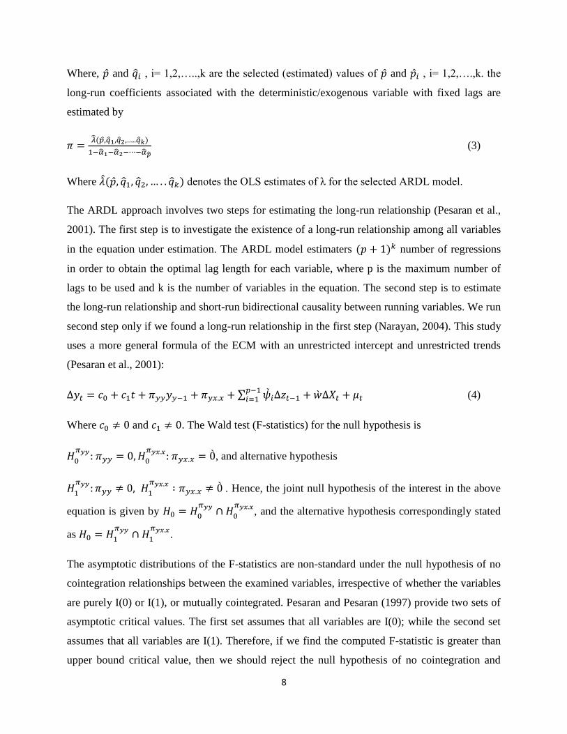
Where, �̂� and �̂�𝑖 , i= 1,2,…..,k are the selected (estimated) values of �̂� and �̂�𝑖 , i= 1,2,….,k. the

long-run coefficients associated with the deterministic/exogenous variable with fixed lags are

estimated by

𝜋 =�̂�(𝑝,�̂�1,�̂�2,…..�̂�𝑘)

1−�̂�1−�̂�2−⋯−�̂��̂� (3)

Where �̂�(�̂�, �̂�1, �̂�2, … . . �̂�𝑘) denotes the OLS estimates of λ for the selected ARDL model.

The ARDL approach involves two steps for estimating the long-run relationship (Pesaran et al.,

2001). The first step is to investigate the existence of a long-run relationship among all variables

in the equation under estimation. The ARDL model estimaters (𝑝 + 1)𝑘 number of regressions

in order to obtain the optimal lag length for each variable, where p is the maximum number of

lags to be used and k is the number of variables in the equation. The second step is to estimate

the long-run relationship and short-run bidirectional causality between running variables. We run

second step only if we found a long-run relationship in the first step (Narayan, 2004). This study

uses a more general formula of the ECM with an unrestricted intercept and unrestricted trends

(Pesaran et al., 2001):

∆𝑦𝑡 = 𝑐0 + 𝑐1𝑡 + 𝜋𝑦𝑦𝑦𝑦−1 + 𝜋𝑦𝑥.𝑥 + ∑ �̀�𝑖∆𝑧𝑡−1𝑝−1𝑖=1 + �̀�∆𝑋𝑡 + 𝜇𝑡 (4)

Where 𝑐0 ≠ 0 and 𝑐1 ≠ 0. The Wald test (F-statistics) for the null hypothesis is

𝐻0

𝜋𝑦𝑦: 𝜋𝑦𝑦 = 0, 𝐻0

𝜋𝑦𝑥.𝑥: 𝜋𝑦𝑥.𝑥 = 0̀, and alternative hypothesis

𝐻1

𝜋𝑦𝑦: 𝜋𝑦𝑦 ≠ 0, 𝐻1

𝜋𝑦𝑥.𝑥 ∶ 𝜋𝑦𝑥.𝑥 ≠ 0̀ . Hence, the joint null hypothesis of the interest in the above

equation is given by 𝐻0 = 𝐻0

𝜋𝑦𝑦 ∩ 𝐻0

𝜋𝑦𝑥.𝑥, and the alternative hypothesis correspondingly stated

as 𝐻0 = 𝐻1

𝜋𝑦𝑦 ∩ 𝐻1

𝜋𝑦𝑥.𝑥.

The asymptotic distributions of the F-statistics are non-standard under the null hypothesis of no

cointegration relationships between the examined variables, irrespective of whether the variables

are purely I(0) or I(1), or mutually cointegrated. Pesaran and Pesaran (1997) provide two sets of

asymptotic critical values. The first set assumes that all variables are I(0); while the second set

assumes that all variables are I(1). Therefore, if we find the computed F-statistic is greater than

upper bound critical value, then we should reject the null hypothesis of no cointegration and

9

conclude that a steady state of equilibrium between the variables exists. If we computed F-

statistic is less than the lower bound critical value, then we could not reject the null of co-

integration. If the computed F-statistic should fall within the lower and upper bound critical

values, then the result would be inconclusive. The model can be selected using the lag length

criteria of Schartz-Criteria (SBC) or Akaike information criteria (AIC).

Following the discussion of theoretical models and the ARDL technique, we employed the

Pesaran et al., (2001) procedure to investigate the existence of a long-run relationship in the form

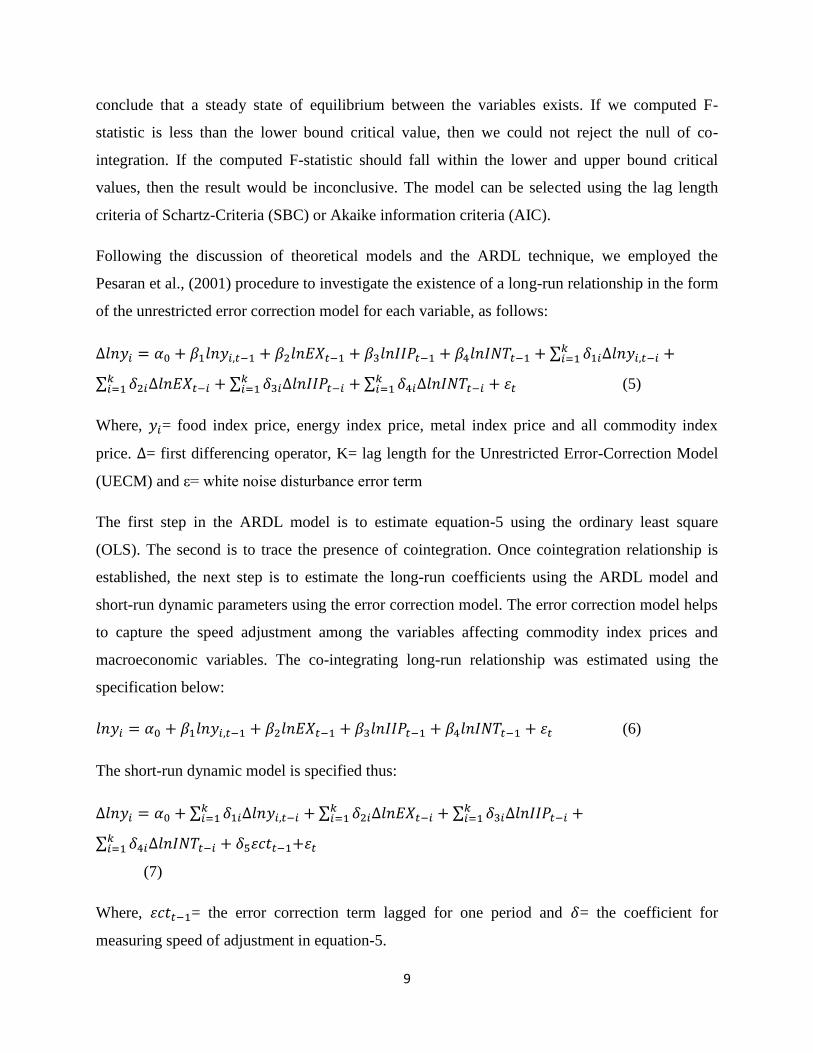
of the unrestricted error correction model for each variable, as follows:

∆𝑙𝑛𝑦𝑖 = 𝛼0 + 𝛽1𝑙𝑛𝑦𝑖,𝑡−1 + 𝛽2𝑙𝑛𝐸𝑋𝑡−1 + 𝛽3𝑙𝑛𝐼𝐼𝑃𝑡−1 + 𝛽4𝑙𝑛𝐼𝑁𝑇𝑡−1 + ∑ 𝛿1𝑖∆𝑙𝑛𝑦𝑖,𝑡−𝑖𝑘𝑖=1 +

∑ 𝛿2𝑖∆𝑙𝑛𝐸𝑋𝑡−𝑖 + ∑ 𝛿3𝑖∆𝑙𝑛𝐼𝐼𝑃𝑡−𝑖𝑘𝑖=1

𝑘𝑖=1 + ∑ 𝛿4𝑖∆𝑙𝑛𝐼𝑁𝑇𝑡−𝑖

𝑘𝑖=1 + 휀𝑡 (5)

Where, 𝑦𝑖= food index price, energy index price, metal index price and all commodity index

price. ∆= first differencing operator, K= lag length for the Unrestricted Error-Correction Model

(UECM) and ε= white noise disturbance error term

The first step in the ARDL model is to estimate equation-5 using the ordinary least square

(OLS). The second is to trace the presence of cointegration. Once cointegration relationship is

established, the next step is to estimate the long-run coefficients using the ARDL model and

short-run dynamic parameters using the error correction model. The error correction model helps

to capture the speed adjustment among the variables affecting commodity index prices and

macroeconomic variables. The co-integrating long-run relationship was estimated using the

specification below:

𝑙𝑛𝑦𝑖 = 𝛼0 + 𝛽1𝑙𝑛𝑦𝑖,𝑡−1 + 𝛽2𝑙𝑛𝐸𝑋𝑡−1 + 𝛽3𝑙𝑛𝐼𝐼𝑃𝑡−1 + 𝛽4𝑙𝑛𝐼𝑁𝑇𝑡−1 + 휀𝑡 (6)

The short-run dynamic model is specified thus:

∆𝑙𝑛𝑦𝑖 = 𝛼0 + ∑ 𝛿1𝑖∆𝑙𝑛𝑦𝑖,𝑡−𝑖𝑘𝑖=1 + ∑ 𝛿2𝑖∆𝑙𝑛𝐸𝑋𝑡−𝑖 + ∑ 𝛿3𝑖∆𝑙𝑛𝐼𝐼𝑃𝑡−𝑖

𝑘𝑖=1

𝑘𝑖=1 +

∑ 𝛿4𝑖∆𝑙𝑛𝐼𝑁𝑇𝑡−𝑖𝑘𝑖=1 + 𝛿5휀𝑐𝑡𝑡−1+휀𝑡

(7)

Where, 휀𝑐𝑡𝑡−1= the error correction term lagged for one period and 𝛿= the coefficient for

measuring speed of adjustment in equation-5.

10

To estimate the values of variables in estimation model, it needs to choose an appropriate lag

length. Though, there are different lag length selection criteria such as the Final Predicted Error

(FPE), Akaike Information Criteria (AIC), Schwartz Information Criteria (SIC) and HQ

(Hendricks Quant) respectively. But we have adopted AIC and SIC to select maximum lag for

the estimation models. But this is relaxed for Johansen cointegration test.

Before examining any linkage between variables, we proceed to check the stationarity of selected

data series using the unit root test.

5. Empirical Interpretations

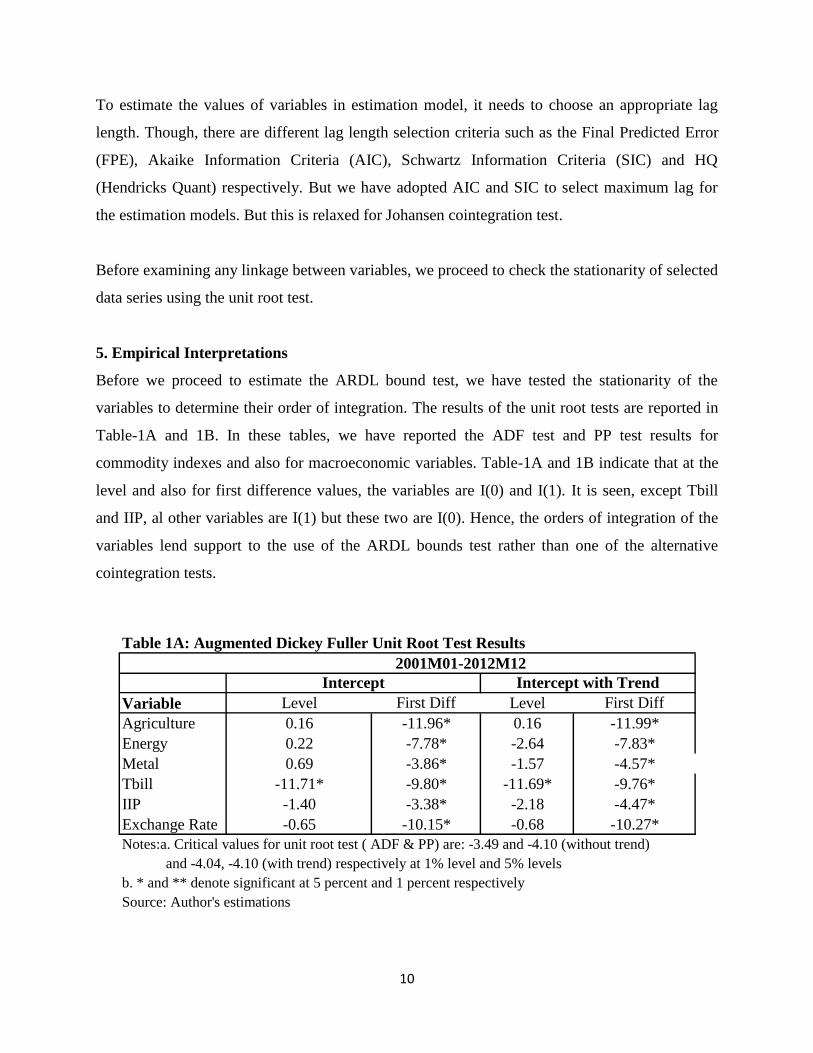
Before we proceed to estimate the ARDL bound test, we have tested the stationarity of the

variables to determine their order of integration. The results of the unit root tests are reported in

Table-1A and 1B. In these tables, we have reported the ADF test and PP test results for

commodity indexes and also for macroeconomic variables. Table-1A and 1B indicate that at the

level and also for first difference values, the variables are I(0) and I(1). It is seen, except Tbill

and IIP, al other variables are I(1) but these two are I(0). Hence, the orders of integration of the

variables lend support to the use of the ARDL bounds test rather than one of the alternative

cointegration tests.

Table 1A: Augmented Dickey Fuller Unit Root Test Results

Variable Level First Diff Level First Diff

Agriculture 0.16 -11.96* 0.16 -11.99*

Energy 0.22 -7.78* -2.64 -7.83*

Metal 0.69 -3.86* -1.57 -4.57*

Tbill -11.71* -9.80* -11.69* -9.76*

IIP -1.40 -3.38* -2.18 -4.47*

Exchange Rate -0.65 -10.15* -0.68 -10.27*

Notes:a. Critical values for unit root test ( ADF & PP) are: -3.49 and -4.10 (without trend)

and -4.04, -4.10 (with trend) respectively at 1% level and 5% levels

b. * and ** denote significant at 5 percent and 1 percent respectively

Source: Author's estimations

Intercept

2001M01-2012M12

Intercept with Trend

11

According to Pesaran et al. (2001), the ARDL cointegration model estimation follows two steps

procedure. Firstly, we have to find out the optimum lag length using the different criteria like

Schwartz Bayesian Criteria (SBC) and Akaike Information Criteria (AIC). Secondly, we have to

estimate the Wald bound test for cointegration. The AIC model suggests that 2 is the optimum

lag for agricultural index price and 3 is the optimum lag for energy and metal index price.

We have estimated the Wald bound test for agriculture index price, energy index price and metal

index price with the selected macroeconomic variables like Tbill, IIP and Exchange rate. The

results of the Wald bound test for cointegration show that the calculated F-statistics are 7785.72,

3843.95 and 3251.57 respectively which are highly significant, led to we reject the null

hypothesis and accept the alternative hypothesis, i.e. there is a cointegration relationship among

the variables in this model. Having found a long-run relationships between commodity index

prices and macroeconomic variables, we have applied the ARDL model to estimate the long-run

and short-run elasticities (Pesaran et al., 2001 and Pesaran and Shin, 1999).

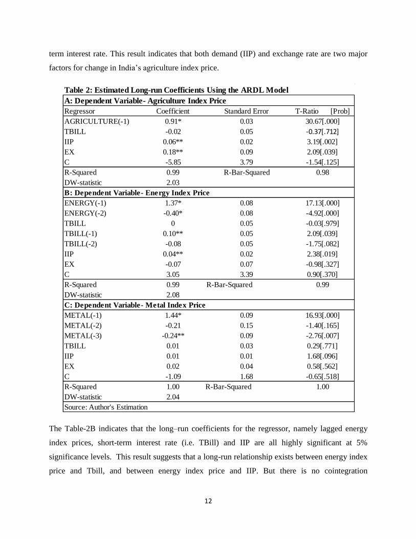
The long-run coefficients of the variables under investigation are shown in the Table-2. The

Table-2 indicates the long-run coefficient estimates for three commodities index price. All the

regression equations are based on the ARDL model selected by the AIC. The Table-2A shows

that the long–run coefficients for the regressor, namely lagged agriculture, iip and exchange rate

are all highly significant at 5% significance levels. This result suggests that a long-run

relationship exists between agriculture index price and iip, and between agriculture and exchange

rate. But there is no co-integration relationship emerged between agriculture and tbill, i.e. short

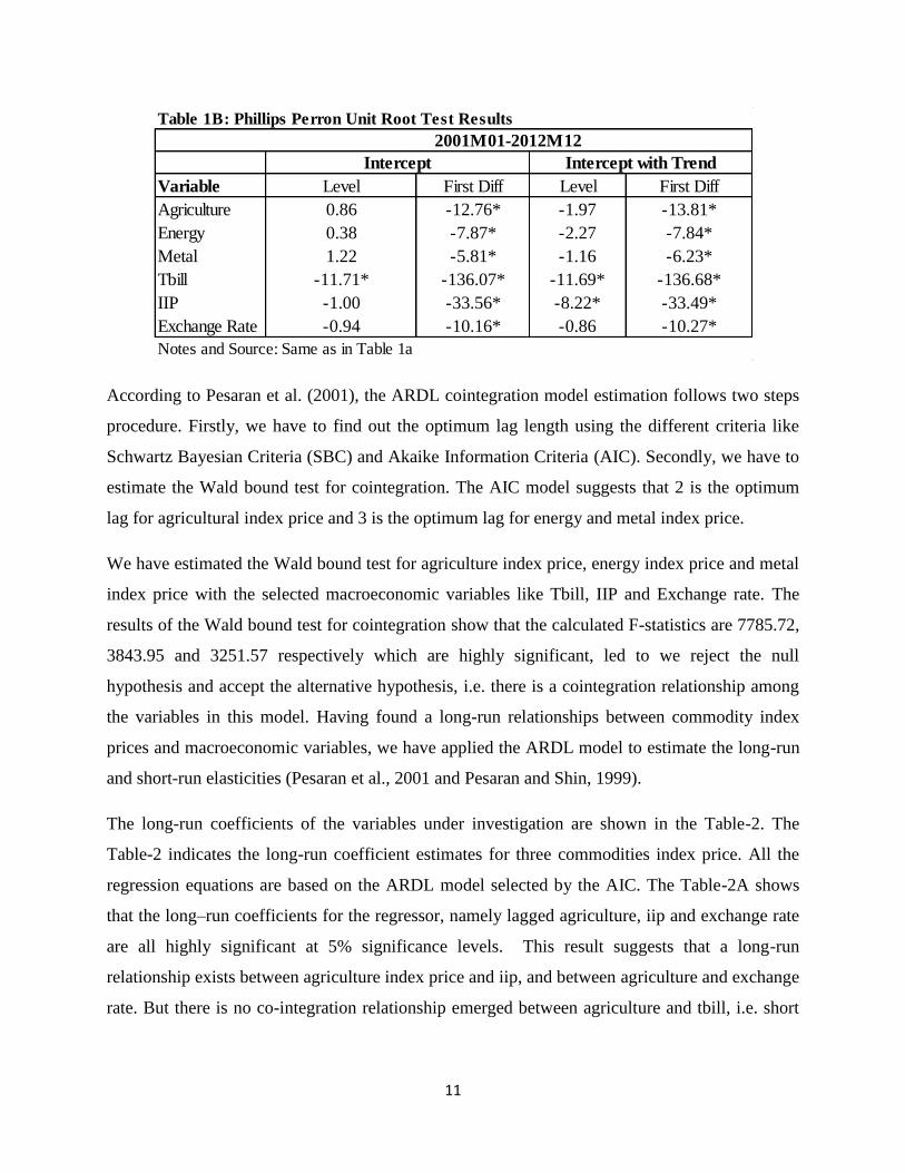
Table 1B: Phillips Perron Unit Root Test Results

Variable Level First Diff Level First Diff

Agriculture 0.86 -12.76* -1.97 -13.81*

Energy 0.38 -7.87* -2.27 -7.84*

Metal 1.22 -5.81* -1.16 -6.23*

Tbill -11.71* -136.07* -11.69* -136.68*

IIP -1.00 -33.56* -8.22* -33.49*

Exchange Rate -0.94 -10.16* -0.86 -10.27*

Notes and Source: Same as in Table 1a

Intercept Intercept with Trend

2001M01-2012M12

12

term interest rate. This result indicates that both demand (IIP) and exchange rate are two major

factors for change in India’s agriculture index price.

The Table-2B indicates that the long–run coefficients for the regressor, namely lagged energy

index prices, short-term interest rate (i.e. TBill) and IIP are all highly significant at 5%

significance levels. This result suggests that a long-run relationship exists between energy index

price and Tbill, and between energy index price and IIP. But there is no cointegration

Table 2: Estimated Long-run Coefficients Using the ARDL Model

A: Dependent Variable- Agriculture Index Price

Regressor Coefficient Standard Error T-Ratio [Prob]

AGRICULTURE(-1) 0.91* 0.03 30.67[.000]

TBILL -0.02 0.05 -0.37[.712]

IIP 0.06** 0.02 3.19[.002]

EX 0.18** 0.09 2.09[.039]

C -5.85 3.79 -1.54[.125]

R-Squared 0.99 R-Bar-Squared 0.98

DW-statistic 2.03

B: Dependent Variable- Energy Index Price

ENERGY(-1) 1.37* 0.08 17.13[.000]

ENERGY(-2) -0.40* 0.08 -4.92[.000]

TBILL 0 0.05 -0.03[.979]

TBILL(-1) 0.10** 0.05 2.09[.039]

TBILL(-2) -0.08 0.05 -1.75[.082]

IIP 0.04** 0.02 2.38[.019]

EX -0.07 0.07 -0.98[.327]

C 3.05 3.39 0.90[.370]

R-Squared 0.99 R-Bar-Squared 0.99

DW-statistic 2.08

C: Dependent Variable- Metal Index Price

METAL(-1) 1.44* 0.09 16.93[.000]

METAL(-2) -0.21 0.15 -1.40[.165]

METAL(-3) -0.24** 0.09 -2.76[.007]

TBILL 0.01 0.03 0.29[.771]

IIP 0.01 0.01 1.68[.096]

EX 0.02 0.04 0.58[.562]

C -1.09 1.68 -0.65[.518]

R-Squared 1.00 R-Bar-Squared 1.00

DW-statistic 2.04

Source: Author's Estimation

13

relationship emerged between energy and exchange rate. This result indicates that both demand

(IIP) and short-term interest rate are two major factors for change in India’s energy index price.

The Table-2C shows that the long–run coefficients for the regressor, namely lag metal index

prices, iip, tbil and exchange rate are insignificant. This result suggests that there is no long-run

relationship exists between metal index price and the macroeconomic variables. But the change

in metal index price is due to some other factors.

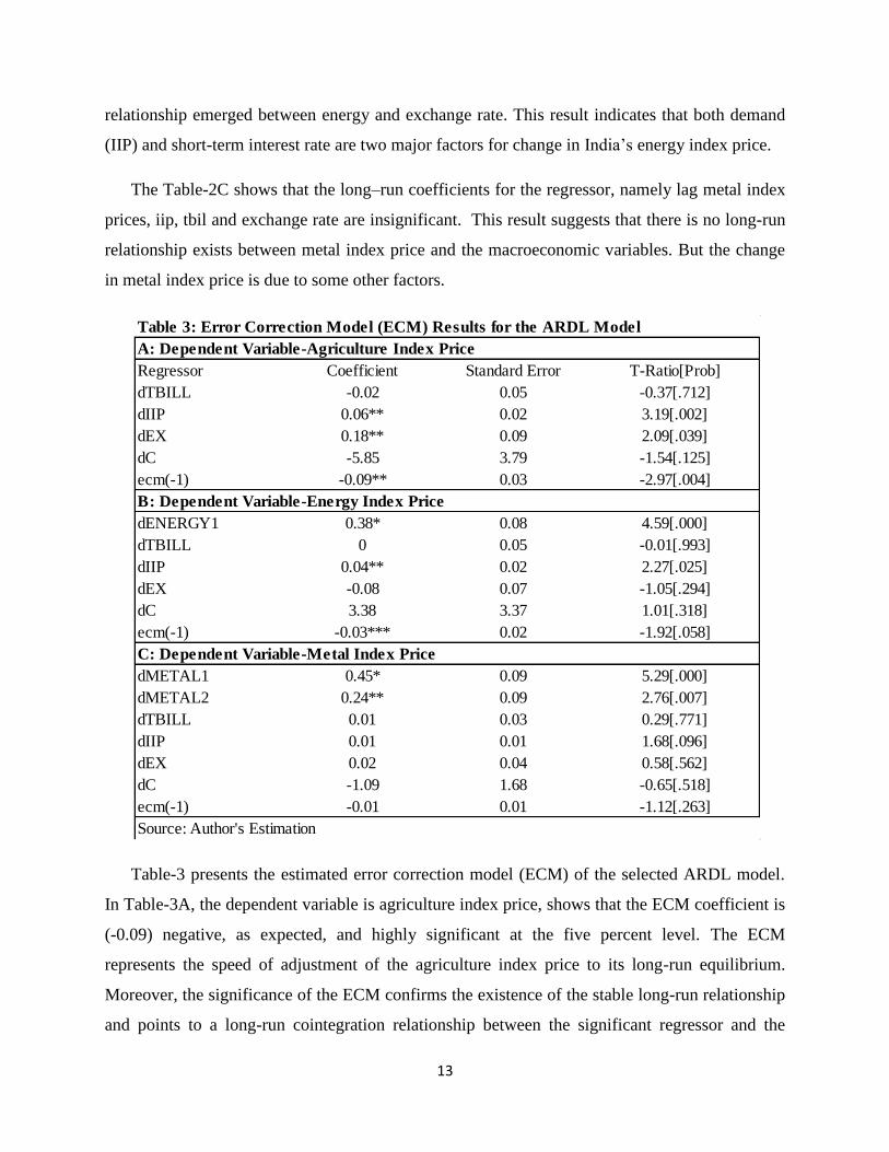
Table-3 presents the estimated error correction model (ECM) of the selected ARDL model.

In Table-3A, the dependent variable is agriculture index price, shows that the ECM coefficient is

(-0.09) negative, as expected, and highly significant at the five percent level. The ECM

represents the speed of adjustment of the agriculture index price to its long-run equilibrium.

Moreover, the significance of the ECM confirms the existence of the stable long-run relationship

and points to a long-run cointegration relationship between the significant regressor and the

Table 3: Error Correction Model (ECM) Results for the ARDL Model

A: Dependent Variable-Agriculture Index Price

Regressor Coefficient Standard Error T-Ratio[Prob]

dTBILL -0.02 0.05 -0.37[.712]

dIIP 0.06** 0.02 3.19[.002]

dEX 0.18** 0.09 2.09[.039]

dC -5.85 3.79 -1.54[.125]

ecm(-1) -0.09** 0.03 -2.97[.004]

B: Dependent Variable-Energy Index Price

dENERGY1 0.38* 0.08 4.59[.000]

dTBILL 0 0.05 -0.01[.993]

dIIP 0.04** 0.02 2.27[.025]

dEX -0.08 0.07 -1.05[.294]

dC 3.38 3.37 1.01[.318]

ecm(-1) -0.03*** 0.02 -1.92[.058]

C: Dependent Variable-Metal Index Price

dMETAL1 0.45* 0.09 5.29[.000]

dMETAL2 0.24** 0.09 2.76[.007]

dTBILL 0.01 0.03 0.29[.771]

dIIP 0.01 0.01 1.68[.096]

dEX 0.02 0.04 0.58[.562]

dC -1.09 1.68 -0.65[.518]

ecm(-1) -0.01 0.01 -1.12[.263]

Source: Author's Estimation

14

agriculture index price. In addition to their long-run cointegration relationship, this result also

suggests that both the IIP and Exchange rate over the previous month had Granger-caused the

agriculture index price.

In Table-3B, the dependent variable is energy index price, shows that the ECM coefficient is

(-0.03) negative and highly significant at the ten percent level. The significance of the ECM

confirms the existence of the stable long-run relationship and points to a long-run cointegration

relationship between the significant regressor and the energy index price. In addition to their

long-run cointegration relationship, this result also suggests that both the energy lagged price and

IIP over the previous month had Granger-caused the energy index price.

In Table-3C, the dependent variable is metal index price, shows that the ECM coefficient is

(-0.01) negative and not significant even at the ten percent level. It confirms that there is no

stable long-run relationship, and points to no long-run cointegration relationship between the

significant regressor and the metal index price. This result also suggests that there is no causality

between metal index price and macroeconomic variables.

6. Conclusion.

This paper examines the relationship between commodities index prices and macroeconomic

variables in India over the period of January 2001 to June 2012 using the time series techniques

of ARDL model and ECM model. The ARDL test suggests that there is long-run cointegration

between the agriculture index price and macroeconomic variables, and also between energy

index price and macroeconomic variables. But, there is no long-run cointegration between metal

index price and macroeconomic variables. The results also indicate that IIP and Exchange rate

have positive and significant effects on agricultural index price. This implies that that IIP and

Exchange rate are vital macroeconomic variables that influence the agricultural index price in the

study period. Similarly, the aggregate demand (i.e. IIP) is the positive and significant effect on

energy index price. This implies that that IIP is a vital macroeconomic variable that influences

the energy index price in the study period. But, there is no such macroeconomic variable we

found which have a significant effect on the metal index price.

15

References

1. Aksoy, M.A. and Beghin, J.C. (ed). Global Agricultural Trade and Developing

Countries. The World Bank, 2005.

2. Alexandratos, N. (2008). Food Price Surges: Possible Causes, Past Experience, and

Longer Term Relevance. Population and Development Review, 34 (4): 663-697.

3. Andersen, T., T. Bollerslev, F. Diebold, and Vega, C. (2003). Micro Effects of Macro

Announcements: Real-Time Price Discovery in Foreign Exchange. American Economic

Review, 93 (1): 38–62.

4. Anderson, K. and Masters, W. (ed). Distortions to Agricultural Incentives in Africa.

The World Bank, 2009.

5. Aregbeyen, O.O. and Ibrahim, T.M. (2012). The Causal Relationship between

Government Spending and Revenue in an Oil-Dependent Economy: the Case of

Nigeria. the IUP Journal of Public Finance, X (1), 6-21.

6. Barnhart, Scott W. (1989). The Effects of Macroeconomic Announcements on

Commodity Prices. American Journal of Agricultural Economics, 71(2): 389-403.

7. Borensztein, E. and Reinhart, C.M. (1994). The Macroeconomic Determinants of

Commodity Prices. IMF Staff Papers, 41: 236-258.

8. Byrne, J., G. Fazio, and Fiess, N. (2011). Primary Commodity Prices: Co-Movements,

Common Factors and Fundamentals. World Bank Policy Research Working Paper, No.

5578.

9. Cai, J., Y. Cheung and Wong, M.C.S. (2001). What Moves the Gold Market?. Journal

of Futures Markets, 21(3): 257-278.

10. Chambers, M. J. and Bailey, R.E. (1996). A Theory of Commodity Price Fluctuations.

Journal of Political Economy, 104 (5): 924-957.

16

11. Christie–David, Rohan, M. Chaudhry, and Koch, T.W. (2000). Do Macroeconomics

News Releases Affect Gold and Silver Prices?. Journal of Economics and Business, 52

(1): 405–421.

12. Commodity Futures Trading Commission (CFTC) report (2008). Swap Dealers and Index

Traders, Staff Report No- PR5542-08.

13. Durnbush, R. (1985). Policy and Performance links between LDC Debtors and

Industrial Nations. Brookings Papers on Economic Activity, 2, 303-368.

14. Dwyer, A., Gardner, G. and Williams, T. (2011). Global Commodity Markets- Price

Volatility and Financialization. Belletin. June Quarter.

15. Erb, C. and Harvey, C. (2006). The Strategic and Tactical Value of Commodity Futures.

Financial Analysts Journal, 62(2): 69–97.

16. Fleming, M. J., & Remolona, E. M. (1999a). Price Formation and Liquidity in the U.S.

Treasury Market: The Response to Public Information. Journal of Finance, 54(5):

1901–1915.

17. Frankel, J.A. (2006). The Effects of Monetary Policy on Real Commodity Prices.

NBER Working Paper, No. 12713.

18. Frankel, J.A. and Hardouvelis, G.A. (1985). Commodity Prices, Money Surprises and

Fed Credibility. Journal of Money, Credit and Banking, 17(4): 425-438.

19. Gilbert, C. L. (1990). The Rational Expectations Hypothesis in Models of Primary

Commodity Prices. World Bank, Policy, Research and External Affairs, Working Paper,

No. 384.

20. Johnson, S. and Juselius, K. (1990). Maximum Likelihood Estimation and Inference on

Cointegration- with Applications to the Demand for Money, Oxford Bulletin of

Economics and Statistics, 52 (2), 169–210.

17

21. Kabia, M.B. and Gil, M. (2000). Short- and Long-run Effects of Macroeconomic

Variables on the Spanish Agricultural Sector. European Review of Agricultural

Economics, 27 (23): 449-471.

22. Kaufmann, R.K. (2011). The Role of Market Fundamentals and Speculation in Recent

Price Changes for Crude oil, Energy Policy, 39 (1), 105-115.

23. Kim, Suk J., Fariboz Moshirian, and Eliza Wu. (2011). Dynamic Stock Market

Integration Driven by the European Monetary Union: An Empirical Analysis. Journal

of Banking and Finance, 29 (10): 2475–2502.

24. Labys, W. C. and Maizels, A. (1990). Commodity Price Fluctuations and Macro-

Economic Adjustments in the Developed Countries. WIDER Working Papers, No.88.

25. Lescaroux, F. (2009). On the Excess Co-movement of Commodity Prices - A Note

about the Role of Fundamental Factors in Short-run Dynamics. Energy Policy, 37(10):

3906-3913.

26. Multi Commodity Exchange Year Book, 2011.

27. Nag, R.N. and Goswami, B. (2008). Macroeconomics of Commodity Price

Fluctuations: A Structuralist Approach. Trade and Development Review, 1 (2): 49-74.

28. Narayan, P.K. (2004). Fiji’s Tourism Demand: the ARDL Approach to Cointegration,

Tourism Economics, 10 (2), 193-206.

29. OECD-FAO Agricultural Outlook 2008-2017.

30. Palaskas, T. and Varangis, P. (1991). Is There Excess Comovement of Primary

Commodity Prices?: A Cointegration Test, World Bank Working Paper, No. 758.

31. Pesaran, M.H., Pesaran, B. (1997). Working with Microfit 4.0: Interactive Econometric

Analysis. United Kingdom: Oxford University Press.

18

32. Pesaran, M.H., Shin, Y., Smith, R.J. (2001). Bounds Testing Approaches to the

Analysis of Level Relationships. Journal of Applied Econometrics, 16 (3), 289-326.

33. Tsay, R.S. (2010). Analysis of Financial Time Series. Wiley, Third Edition.

34. UNCTAD. (2009), Trade and Development Report, 2009

35. UNCTAD. (2009). The Growing Interdependence between Financial and Commodity

Markets. Discussion Paper, No. 195.

36. UNCTAD. (2010). Recent Commodity Market Developments: Trends and Challenges.

Geneva, TD/B/C.1/MEM.2/7.

37. UNCTAD. (2011). Price Formation in Financialized Commodity Markets: The Role of

Information. United Nations, New York and Geneva.

38. UNCTAD Discussion Paper 197, March 2010.

39. Zahid, S., A. Qayyum and Shahid, W. (2007). Dynamics of Wheat Market Integration

in Northern Punjab, Pakistan. The Pakistan Development Review, 46(4): 817-830.

40. Zanias, G.P. (1993). Testing for Integration in European Community Agricultural

Product Markets. Journal of Agricultural Economics, 44(3): 418–427.

Appendix

A.1: Construction of Commodity Price Index

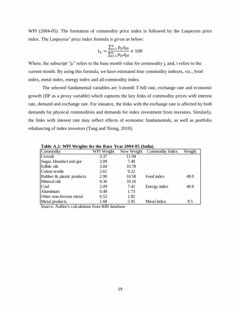
In this chapter, we have constructed a specific commodity price index to assess the impact of

fundamental variables on commodity prices. While constructing the commodity price index, we

capture the relative importance of the commodity for India using the weight of the commodity in

the WPI basket (base 2004-05). In Table-1, we have reported the commodity price weight in

19

WPI (2004-05). The formation of commodity price index is followed by the Laspeyres price

index. The Laspeyres’ price index formula is given as below:

Lt =∑ pjtqj0

nj=1

∑ pjoqj0nj=1

× 100

Where, the subscript “j0” refers to the base month value for commodity j, and, t refers to the

current month. By using this formula, we have estimated four commodity indexes, viz., food

index, metal index, energy index and all-commodity index.

The selected fundamental variables are 3-month T-bill rate, exchange rate and economic

growth (IIP as a proxy variable) which captures the key links of commodity prices with interest

rate, demand and exchange rate. For instance, the links with the exchange rate is affected by both

demands for physical commodities and demands for index investment from investors. Similarly,

the links with interest rate may reflect effects of economic fundamentals, as well as portfolio

rebalancing of index investors (Tang and Xiong, 2010).

Table A.2: WPI Weights for the Base Year 2004-05 (India)

Commodity WPI Weight New Weight Commodity Index WeightCereals 3.37 11.94Sugar, khandari and gur 2.09 7.40Edible oils 3.04 10.78Cotton textile 2.61 9.22Rubber & plastic products 2.99 10.58 Food index 49.9Mineral oils 9.36 33.16Coal 2.09 7.42 Energy index 40.6Aluminium 0.49 1.73Other non-ferrous metal 0.52 1.82Metal products 1.68 5.95 Metal index 9.5Source: Author's calculations from RBI database