multivariate garch models: a survey - cass.city.ac.uk garch models: ... (arch) models are now...

JOURNAL OF APPLIED ECONOMETRICSJ. Appl. Econ. 21: 79–109 (2006)Published online in Wiley InterScience (www.interscience.wiley.com). DOI: 10.1002/jae.842

MULTIVARIATE GARCH MODELS: A SURVEY

LUC BAUWENS,a* SEBASTIEN LAURENTb AND JEROEN V. K. ROMBOUTSa

a CORE and Department of Economics, Universite catholique de Louvain, Belgiumb CeReFim, Universite de Namur and CORE, Universite catholique de Louvain, Belgium

SUMMARYThis paper surveys the most important developments in multivariate ARCH-type modelling. It reviews themodel specifications and inference methods, and identifies likely directions of future research. Copyright 2006 John Wiley & Sons, Ltd.

1. INTRODUCTION

Understanding and predicting the temporal dependence in the second-order moments of assetreturns is important for many issues in financial econometrics. It is now widely accepted thatfinancial volatilities move together over time across assets and markets. Recognizing this featurethrough a multivariate modelling framework leads to more relevant empirical models than workingwith separate univariate models. From a financial point of view, it opens the door to better decisiontools in various areas, such as asset pricing, portfolio selection, option pricing, hedging and riskmanagement. Indeed, unlike at the beginning of the 1990s, several institutions have now developedthe necessary skills to use the econometric theory in a financial perspective.

Since the seminal paper of Engle (1982), traditional time series tools such as autoregressivemoving average (ARMA) models (Box and Jenkins, 1970) for the mean have been extendedto essentially analogous models for the variance. Autoregressive conditional heteroscedasticity(ARCH) models are now commonly used to describe and forecast changes in the volatility offinancial time series. For a survey of ARCH-type models, see Bollerslev et al. (1992, 1994), Beraand Higgins (1993), Pagan (1996), Palm (1996) and Shephard (1996), among others.

The most obvious application of MGARCH (multivariate GARCH) models is the study of therelations between the volatilities and co-volatilities of several markets.1 Is the volatility of a marketleading the volatility of other markets? Is the volatility of an asset transmitted to another assetdirectly (through its conditional variance) or indirectly (through its conditional covariances)? Doesa shock on a market increase the volatility on another market, and by how much? Is the impactthe same for negative and positive shocks of the same amplitude? A related issue is whether thecorrelations between asset returns change over time.2 Are they higher during periods of highervolatility (sometimes associated with financial crises)? Are they increasing in the long run, perhapsbecause of the globalization of financial markets? Such issues can be studied directly by usinga multivariate model, and raise the question of the specification of the dynamics of covariancesor correlations. In a slightly different perspective, a few papers have used MGARCH models to

Ł Correspondence to: Luc Bauwens, CORE, 34 Voie du Roman Pays, B-1348 Louvain-La-Neuve, Belgium.E-mail: [email protected] Kearney and Patton (2000) and Karolyi (1995) exemplify such studies.2 See Bollerslev (1990) and Longin and Solnik (1995).

Copyright 2006 John Wiley & Sons, Ltd. Received 22 April 2003Revised 3 June 2004

80 L. BAUWENS, S. LAURENT AND J. V. K. ROMBOUTS

assess the impact of volatility in financial markets on real variables like exports and output growthrates, and the volatility of these growth rates.3

Another application of MGARCH models is the computation of time-varying hedge ratios.Traditionally, constant hedge ratios are estimated by OLS as the slope of a regression of the spotreturn on the futures return, because this is equivalent to estimating the ratio of the covariancebetween spot and futures over the variance of the futures. Since a bivariate MGARCH model for thespot and futures returns directly specifies their conditional variance–covariance matrix, the hedgeratio can be computed as a byproduct of estimation and updated by using new observations as theybecome available. See Lien and Tse (2002) for a survey on hedging and additional references.

Asset pricing models relate returns to ‘factors’, such as the market return in the capital assetpricing model. A specific asset excess return (in excess of the risk-free return) may be expressedas a linear function of the market return. Assuming its constancy, the slope, or ˇ coefficient, maybe estimated by OLS. Like in the hedging case, since the ˇ is the ratio of a covariance to avariance, an MGARCH model can be used to estimate time-varying ˇ coefficients. See Bollerslevet al. (1988), De Santis and Gerard (1998), Hafner and Herwartz (1998) for examples.

Given an estimated univariate GARCH model on a return series, one knows the returnconditional distribution, and one can forecast the value-at-risk (VaR) of a long or short position.When considering a portfolio of assets, the portfolio return can be computed directly from theasset shares and returns. A GARCH model can be fit to the portfolio returns for given weights. Ifthe weight vector changes, the model has to be estimated again. On the contrary, if a multivariateGARCH model is fitted, the multivariate distribution of the returns can be used directly to computethe implied distribution of any portfolio. There is no need to re-estimate the model for differentweight vectors. In the present state of the art, it is probably simpler to use the univariate frameworkif there are many assets, but we conjecture that using a multivariate specification may becomea feasible alternative. Whether the univariate ‘repeated’ approach is more adequate than themultivariate one is an open question. The multivariate approach is illustrated by Giot and Laurent(2003) using a trivariate example with a time-varying correlation model.

MGARCH models were initially developed in the late 1980s and the first half of the 1990s, andafter a period of tranquillity in the second half of the 1990s, this area seems to be experiencingagain a quick expansion phase. MGARCH models are partly covered in Franses and van Dijk(2000), Gourieroux (1997) and most of the surveys on ARCH models cited above, but none ofthem presents, as this one, a comprehensive and up-to-date survey of the field, including the mostrecent findings.

The paper is organized in the following way. In Section 2, we review existing MGARCHspecifications. Section 3 is devoted to estimation problems and Section 4 to diagnostic tests.Finally, we offer our conclusions and ideas for further developments in Section 5.

2. OVERVIEW OF MODELS

Consider a vector stochastic process fytg of dimension Nð 1. As usual, we condition on the sigmafield, denoted by It�1, generated by the past information (here the yt’s) until time t � 1. We denoteby � a finite vector of parameters and write:

yt D �t��C εt �1�

3 See Kim (2000).

Copyright 2006 John Wiley & Sons, Ltd. J. Appl. Econ. 21: 79–109 (2006)

MULTIVARIATE GARCH MODELS 81

where �t�� is the conditional mean vector and

εt D H1/2t ��zt �2�

where H1/2t �� is a NðN positive definite matrix. Furthermore, we assume the Nð 1 random

vector zt to have the following first two moments:

E�zt� D 0

Var�zt� D IN �3�

where IN is the identity matrix of order N. We still have to explain what H1/2t is (for convenience

we leave out � in the notation). To make this clear we calculate the conditional variance matrixof yt:

Var�ytjIt�1� D Vart�1�yt� D Vart�1�εt�

D H1/2t Vart�1�zt��H

1/2t �0

D Ht �4�

Hence H1/2t is any NðN positive definite matrix such that Ht is the conditional variance matrix

of yt, e.g. H1/2t may be obtained by the Cholesky factorization of Ht. Both Ht and �t depend

on the unknown parameter vector �, which can in most cases be split into two disjoint parts, onefor �t and one for Ht.4 A case where this is not true is that of GARCH-in-mean models, where�t is functionally dependent on Ht. In this section, we take no account of the conditional meanvector for notational ease. It is usually specified as a function of the past, through a vectorialautoregressive moving average (VARMA) representation for the level of yt.

In the following subsections we review different specifications of Ht. They differ in variousaspects. We distinguish three nonmutually exclusive approaches for constructing multivariateGARCH models; (i) direct generalizations of the univariate GARCH model of Bollerslev (1986);(ii) linear combinations of univariate GARCH models; (iii) nonlinear combinations of univariateGARCH models. In the first category we have VEC, BEKK and factor models. Related modelslike the flexible MGARCH, Riskmetrics, Cholesky and full factor GARCH models are also inthis category. In the second category we have (generalized) orthogonal models and latent factormodels. The last category contains constant and dynamic conditional correlation models, thegeneral dynamic covariance model and copula-GARCH models. To keep the notational burdenlow, we present the models in their ‘(1,1)’ form rather than in their general ‘(p,q)’ form.

2.1. Generalizations of the Univariate Standard GARCH Model

The models in this category are multivariate extensions of the univariate GARCH model. When weconsider VARMA models for the conditional mean of several time series the number of parametersincreases rapidly. The same happens for multivariate GARCH models as straightforward extensionsof the univariate GARCH model. Furthermore, since Ht is a variance matrix, positive definitenesshas to be ensured. To make the model tractable for applied purposes, additional structure may be

4 Note that although the GARCH parameters do not affect the conditional mean, the conditional mean parameters generallyenter the conditional variance specification through the residuals.



imposed, for example in the form of factors or diagonal parameter matrices. This class of modelslends itself to relatively easy theoretical derivations of stationarity and ergodicity conditions, andunconditional moments (see e.g. He and Terasvirta, 2002a).

VEC and BEKK ModelsA general formulation of Ht has been proposed by Bollerslev et al. (1988). In the general VECmodel, each element of Ht is a linear function of the lagged squared errors and cross-products oferrors and lagged values of the elements of Ht.

Definition 1 The VEC(1, 1) model is defined as:

ht D c C A�t�1 CGht�1 �5�

where

ht D vech�Ht� �6�

�t D vech�εtε0t� �7�

and vech�Ð� denotes the operator that stacks the lower triangular portion of a NðN matrix as aN�NC 1�/2 ð 1 vector. A and G are square parameter matrices of order �NC 1�N/2 and c is a�NC 1�N/2 ð 1 parameter vector.

The number of parameters is N�NC 1��N�NC 1�C 1�/2 (e.g. for N D 3 it is equal to 78), whichimplies that in practice this model is used only in the bivariate case. To overcome this problemsome simplifying assumptions have to be imposed. Bollerslev et al. (1988) suggest the diagonalVEC (DVEC) model in which the A and G matrices are assumed to be diagonal, each elementhijt depending only on its own lag and on the previous value of εitεjt. This restriction reducesthe number of parameters to N�NC 5�/2 (e.g. for N D 3 it is equal to 12). But even under thisdiagonality assumption, large-scale systems are still highly parameterized and difficult to estimatein practice.

Necessary and sufficient conditions on the parameters to ensure that the conditional variancematrices in the DVEC model are positive definite almost surely are most easily derived byexpressing the model in terms of Hadamard products (denoted by þ).5 In particular, let usdefine the symmetric NðN matrices A°, G° and C° as the matrices implied by the relationsA D diag[vech�A°�],6 G D diag[vech�G°�] and c D vech�C°�. The diagonal model can thus bewritten as follows:

Ht D C° C A° þ �εt�1ε0t�1�CG° þHt�1 �8�

It is straightforward to show (see Attanasio, 1991) that Ht is positive definite for all t provided thatC°, A°, G° and the initial variance matrix �H0� are positive definite. Moreover, these conditionsare easily imposed through a Cholesky decomposition of the parameter matrices in (8). Notethat even simpler versions of the DVEC model constrain the A° and G° matrices to be rank one

5 If A D �aij� and B D �bij� are both mð n matrices, then Aþ B is the mð n matrix containing elementwise products�aijbij�.6 If v is a vector of dimension m then diag(v) is the mð m diagonal matrix with v on the main diagonal.



matrices, or a positive scalar times a matrix of ones, also called a scalar model (see Ding andEngle, 2001).

Riskmetrics (1996) uses the exponentially weighted moving average model (EWMA) to forecastvariances and covariances. Practitioners who study volatility processes often observe that theirmodel is very close to the unit root case. To take this into account, Riskmetrics defines thevariances and covariances as IGARCH-type models (Engle and Bollerslev, 1986):

hij,t D �1 � ��εi,t�1εj,t�1 C �hij,t�1 �9�

In terms of the VEC model in (5) we have

ht D �1 � ��t�1 C �ht�1 �10�

which is a scalar VEC model. The decay factor � proposed by Riskmetrics is equal to 0.94 for dailydata and 0.97 for monthly data. The decay factor is not estimated but suggested by Riskmetrics.In this respect, the model is easy to work with in practice. However, imposing the same dynamicson every component in a multivariate GARCH model, no matter which data are used, is difficultto justify.

Because it is difficult to guarantee the positivity of Ht in the VEC representation without impos-ing strong restrictions on the parameters,7 Engle and Kroner (1995) propose a new parametrizationforHt that easily imposes its positivity, i.e. the BEKK model (the acronym comes from synthesizedwork on multivariate models by Baba, Engle, Kraft and Kroner).

Definition 2 The BEKK(1, 1, K) model is defined as:

Ht D CŁ0CŁ C

K∑kD1

AŁ0k εt�1ε

0t�1A

Łk C

K∑kD1

GŁ0k Ht�1G

Łk �11�

where CŁ, AŁk and GŁ

k are NðN matrices but CŁ is upper triangular.

The summation limit K determines the generality of the process. The parameters of the BEKKmodel do not represent directly the impact of the different lagged terms on the elements of Ht,like in the VEC model. The BEKK model is a special case of the VEC model. We refer to Engleand Kroner (1995) for propositions and proofs about VEC and BEKK models. For example, toavoid observationally equivalent structures they provide sufficient conditions to identify BEKKmodels with K D 1. These conditions are that AŁ

k,11, GŁk,11 and the diagonal elements of CŁ are

restricted to be positive.The number of parameters in the BEKK(1,1,1) model is N�5NC 1�/2. To reduce this number,

and consequently to reduce the generality, one can impose a diagonal BEKK model, i.e. AŁk and

GŁk in (11) are diagonal matrices. This model is also a DVEC model but it is less general, although

it is guaranteed to be positive definite while the DVEC is not. This can again be easily checkedin the bivariate model: the DVEC model contains 9 parameters while the BEKK model containsonly 7 parameters. This happens because the parameters governing the dynamics of the covarianceequation in the BEKK model are the products of the corresponding parameters of the two variance

7 Gourieroux (1997, section 6.1) gives sufficient conditions for the positivity of Ht. These conditions are obtained bywriting the model for the matrix Ht itself rather than for its vectorized version.



equations in the same model. Another way to reduce the number of parameters is to use a scalarBEKK model, i.e. AŁ

k and GŁk are equal to a scalar times a matrix of ones.

For the VEC model in Definition 1 to be covariance-stationary it is required that the eigenvaluesof ACG are less than one in modulus. The unconditional variance matrix , equal to E�Ht�,is given by vech�� D [INŁ � A�G]�1

c , where NŁ D N�NC 1�/2. Similar expressions can beobtained for the BEKK model. Hafner (2003) provides analytical expressions of the fourth-ordermoments of the general VEC model; see also Nijman and Sentana (1996).

Besides the BEKK model, another option to guarantee the positivity of Ht in the VECrepresentation is given by Kawakatsu (2003), who proposes the Cholesky factor GARCH model.Instead of specifying a functional form for Ht, he specifies a model on Lt where Ht D LtL0

t. Theadvantage of this specification is that Ht is always positive definite without any restrictions onthe parameters. The disadvantage is that identification restrictions are needed, which implies thatthe order of the series in yt is relevant and that the interpretation of the parameters is difficult.A similar model based on the Cholesky decomposition can be found in Gallant and Tauchen(2001) and in Tsay (2002).

The difficulty when estimating a VEC or even a BEKK model is the high number of unknownparameters, even after imposing several restrictions. It is thus not surprising that these modelsare rarely used when the number of series is larger than 3 or 4. Factor and orthogonal modelscircumvent this difficulty by imposing a common dynamic structure on all the elements of Ht,which results in less parameterized models.

Factor ModelsEngle et al. (1990b) propose a parameterization of Ht using the idea that co-movements of thestock returns are driven by a small number of common underlying variables, which are calledfactors. Bollerslev and Engle (1993) use this parametrization to model common persistence inconditional variances. The factor model can be seen as a particular BEKK model. We take thedefinition of Lin (1992).

Definition 3 The BEKK(1, 1, K) model in Definition 2 is a factor GARCH model, denoted byF-GARCH(1, 1, K), if for each k D 1, . . . , K, AŁ

k and GŁk have rank one and have the same left and

right eigenvectors,8 �k and wk , i.e.

AŁk D ˛kwk�

0k and GŁ

k D ˇkwk�0k, �12�

where ˛k and ˇk are scalars, and �k and wk (for k D 1, . . . , K) are Nð 1 vectors satisfying

w0k�i D

{0 for k 6D i1 for k D i

�13�

N∑nD1

wkn D 1 �14�

8 A 1 ð m vector v 6D 0 satisfying vA D �v for an mð m matrix A and a complex number � is a left eigenvector of Acorresponding to the eigenvalue �, see Lutkepohl (1996, p. 256).



If we substitute (12) and (13) into (11) and define D CŁ0CŁ, we get

Ht D CK∑kD1

�k�0k�˛

2kw

0kεt�1ε

0t�1wk C ˇ2

kw0kHt�1wk� �15�

Restriction (14) is an identification restriction. The K-factor GARCH model implies that the time-varying part of Ht has reduced rank K, but Ht remains of full rank because is assumed positivedefinite. The vector �k and the scalar w0

kεt (denoted by fkt hereafter) are also called the kth factorloading and the kth factor, respectively. The number of parameters in the F-GARCH(1, 1, 1) isN�NC 5�/2. In (15), the expression between brackets can be replaced by other univariate GARCHspecifications.

For example, the conditional variance matrix of the F-GARCH (1, 1, 2) model is:

Ht D C �1�01[˛2

1w01εt�1ε

0t�1w1 C ˇ2

1w01Ht�1w1] C �2�

02[˛2

2w02εt�1ε

0t�1w2 C ˇ2

2w02Ht�1w2] �16�

where the parameter vectors �k D ��k1, �k2, . . . , �kN�0 and wk are of dimension Nð 1 while ˛2k and

ˇ2k are scalar parameters. Denoting 2

k,t D w0kHtwk we can write (16) in a more familiar way as:

hijt D �ij C �1i�1j1t C �2i�2j2t 8i, j D 1, . . . , N �17�

2k,t D ωk C ˛2

kf2k,t�1 C ˇ2

k2k,t�1 k D 1, 2 �18�

where �ij D ωij � �1i�1jω1 � �2i�2jω2 and ωk D w0kwk . Hence kt is defined as a univariate

GARCH(1, 1) model. The persistence of the conditional variance in (16) is measured by∑2kD1�˛

2k C ˇ2

k � and can also be interpreted as common persistence. In other words, the dynamicsof the elements of Ht is the same. We can write Ht as:

Ht D Ł C �1�01

21,t C �2�

02

22,t �19�

where Ł D � �1�01ω1 � �2�0

2ω2. Note that Et�1�f1tf2t� D ω01w2 because ω0

k�l D 0 for k 6D l,see (13). This implies that in the case of more than one factor we have the result that any pair offactors has a time-invariant conditional covariance.

Alternatively, the two-factor model described in (19) can be obtained from

εt D �1f1t C �2f2t C et �20�

where et represents an idiosyncratic shock with constant variance matrix and uncorrelated with thetwo factors. Each factor fkt has zero conditional mean and conditional variance like a GARCH(1,1)process, see (18). The K-factor model can be written as

εt D ft C et �21�

where is a matrix of dimension Nð K and ft is a Kð 1 vector. A factor is observable ifit is specified as a function of εt, like in (16). See Section 2.6 for a brief discussion of latentfactor models.

Several variants of the factor model are proposed in the literature. For example, Vrontos et al.(2003) introduce the full-factor multivariate GARCH model.



Definition 4 The FF-MGARCH model is defined as

Ht D WtW0 �22�

where W is a NðN triangular parameter matrix with ones on the diagonal and the matrixt D diag�2

1,t, . . . , 2N,t� where 2

i,t is the conditional variance of the ith factor, i.e. the ith elementof W�1εt, which can be separately defined as any univariate GARCH model.

By construction, Ht is always positive definite. Note that Ht has a structure that depends on theordering of the time series in yt, because of the triangular structure of W. The restriction of havingones on the diagonal of W avoids superfluous parameters if each 2

i,t has a free constant term.Rigobon and Sack (2003) start from a system of simultaneous equations in structural form

where the conditional variances of the innovations are jointly specified. By deriving the reducedform model one obtains innovations with a conditional variance matrix that can be compared withother unrestricted reduced-form MGARCH models. The structural model imposes a number ofrestrictions on the functional form of the conditional variance of the reduced-form innovations,resulting in less parameters than in a VEC model.

2.2. Linear Combinations of Univariate GARCH Models

In this category, we consider models, like orthogonal models and latent factor models (brieflydiscussed in Section 2.6), that are linear combinations of several univariate models, each of whichis not necessarily a standard GARCH (e.g. the EGARCH model of Nelson (1991), the APARCHmodel of Ding et al. (1993), the fractionally integrated GARCH of Baillie et al. (1996), thecontemporaneous asymmetric GARCH model of El Babsiri and Zakoian (2001) or the quadraticARCH model of Sentana (1995)).

In the orthogonal GARCH model, the observed data are assumed to be generated by anorthogonal transformation of N (or a smaller number of) univariate GARCH processes. Thematrix of the linear transformation is the orthogonal matrix (or a selection) of eigenvectors ofthe population unconditional covariance matrix of the standardized returns. In the generalizedversion, this matrix must only be invertible. The orthogonal models can also be considered asfactor models, where the factors are univariate GARCH-type processes.

In the orthogonal GARCH model of Kariya (1988) and Alexander and Chibumba (1997), theNðN time-varying variance matrix Ht is generated by m � N univariate GARCH models.

Definition 5 The O-GARCH(1,1, m) model is defined as:

V�1/2εt D ut D mft �23�

where V D diag�v1, v2, . . . , vN�, with vi the population variance of εit, and m is a matrix ofdimension Nð m given by:

m D Pm diag�l1/21 . . . l1/2m � �24�

l1 ½ . . . ½ lm > 0 being the m largest eigenvalues of the population correlation matrix of ut, and Pmthe Nð m matrix of associated (mutually orthogonal) eigenvectors. The vector ft D �f1t . . . fmt�0



is a random process such that:

Et�1�ft� D 0 and Vart�1�ft� D t D diag�2f1t, . . . ,

2fmt� �25�

2fit D �1 � ˛i � ˇi�C ˛if

2i,t�1 C ˇi

2fi,t�1

i D 1, . . . , m �26�

Consequently,

Ht D Vart�1�εt� D V1/2VtV1/2 where Vt D Vart�1�ut� D mt

0m �27�

The parameters of the model are V, m and the parameters of the GARCH factors (˛i’s and ˇi’s).The number of parameters is N�NC 5�/2 (if m D N). In practice, V and m are replaced by theirsample counterparts, and m is chosen by principal component analysis applied to the standardizedresiduals Out. Alexander (2001, section 7.4.3) illustrates the use of the O-GARCH model. Sheemphasizes that using a small number of principal components compared to the number of assetsis the strength of the approach (in one example, she fixes m at 2 for 12 assets). However, notethat the conditional variance matrix has reduced rank (if m < N), which may be a problem forapplications and for diagnostic tests which depend on the inverse of Ht.

In van der Weide (2002) the orthogonality condition assumed in the O-GARCH model is relaxedby assuming that the matrix in the relation ut D ft is square and invertible, rather thanorthogonal. The matrix has N2 parameters and is not restricted to be triangular like in themodel of Vrontos et al. (2003), see Definition 4.

Definition 6 The GO-GARCH(1, 1) model is defined as in Definition 5, where m D N and is a nonsingular matrix of parameters. The implied conditional correlation matrix of εt can beexpressed as:

Rt D J�1t VtJ

�1t where Jt D �Vt þ Im�

1/2and Vt D t0 �28�

In van der Weide (2002), the singular value decomposition of the matrix is used as aparametrization, i.e. D PL1/2U, where the matrix U is orthogonal, and P and L are defined asabove (from the eigenvectors and eigenvalues). The O-GARCH model (when m D N) correspondsthen to the particular choice U D IN. More generally, van der Weide expresses U as the productof N�N� 1�/2 rotation matrices:

U D∏i<j

Gij�υij� � � � υij � �, i, j D 1, 2, . . . n �29�

where Gij�υij� performs a rotation in the plane spanned by the ith and jth vectors of the canonicalbasis of IRN over an angle υij. For example, in the trivariate case

G12 D( cos υ12 sin υ12 0

� sin υ12 cos υ12 00 0 1

),G13 D

( cos υ13 0 � sin υ13

0 1 0� sin υ13 0 cos υ13

)�30�

and G23 has the block with cos υ23 and sin υ23 functions in the lower right corner. The N�N� 1�/2rotation angles are parameters to be estimated.



For estimation, van der Weide (2002) replaces in a first step P and L by their sample counterpartsand the remaining parameters (those of U) are estimated together with the parameters of theGARCH factors in a second step. Note that such a two-step estimation method is not applicableif an MGARCH-in-mean effect is included (this is also the case for the O-GARCH model). Moregenerally, as pointed out by a referee, the elements in the matrix could be estimated togetherwith the GARCH parameters of the factors, in a single step.

The orthogonal models are particular F-GARCH models and thus are nested in the BEKKmodel. As a consequence, their properties follow from those of the BEKK model. In particular,it is obvious that the (G)O-GARCH model is covariance-stationary if the m univariate GARCHprocesses are themselves stationary.

2.3. Nonlinear Combinations of Univariate GARCH Models

This section collects models that may be viewed as nonlinear combinations of univariate GARCHmodels. This allows for models where one can specify separately, on the one hand, the individualconditional variances, and on the other hand, the conditional correlation matrix or another measureof dependence between the individual series (like the copula of the conditional joint density). Formodels of this category, theoretical results on stationarity, ergodicity and moments may not beso straightforward to obtain as for models presented in the preceding sections. Nevertheless, theyare less greedy in parameters than the models of the first category, and therefore they are moreeasily estimable.

Conditional Correlation ModelsThe conditional variance matrix for this class of models is specified in a hierarchical way.First, one chooses a GARCH-type model for each conditional variance. For example, someconditional variances may follow a conventional GARCH model while others may be describedas an EGARCH model. Second, based on the conditional variances one models the conditionalcorrelation matrix (imposing its positive definiteness 8t).

Bollerslev (1990) proposes a class of MGARCH models in which the conditional correlations areconstant and thus the conditional covariances are proportional to the product of the correspondingconditional standard deviations. This restriction greatly reduces the number of unknown parametersand thus simplifies the estimation.

Definition 7 The CCC model is defined as:

Ht D DtRDt D ��ij√hiithjjt� �31�

whereDt D diag�h1/2

11t . . . h1/2NNt� �32�

hiit can be defined as any univariate GARCH model, and

R D ��ij� �33�

is a symmetric positive definite matrix with �ii D 1, 8i.Copyright 2006 John Wiley & Sons, Ltd. J. Appl. Econ. 21: 79–109 (2006)


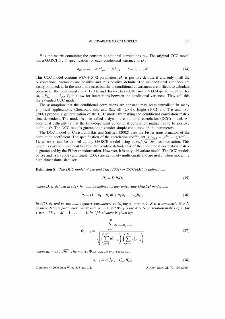
R is the matrix containing the constant conditional correlations �ij. The original CCC modelhas a GARCH(1, 1) specification for each conditional variance in Dt:

hiit D ωi C ˛iε2i,t�1 C ˇihii,t�1 i D 1, . . . , N �34�

This CCC model contains N�NC 5�/2 parameters. Ht is positive definite if and only if all theN conditional variances are positive and R is positive definite. The unconditional variances areeasily obtained, as in the univariate case, but the unconditional covariances are difficult to calculatebecause of the nonlinearity in (31). He and Terasvirta (2002b) use a VEC-type formulation for�h11t, h22t, . . . , hNNt�0, to allow for interactions between the conditional variances. They call thisthe extended CCC model.

The assumption that the conditional correlations are constant may seem unrealistic in manyempirical applications. Christodoulakis and Satchell (2002), Engle (2002) and Tse and Tsui(2002) propose a generalization of the CCC model by making the conditional correlation matrixtime-dependent. The model is then called a dynamic conditional correlation (DCC) model. Anadditional difficulty is that the time-dependent conditional correlation matrix has to be positivedefinite 8t. The DCC models guarantee this under simple conditions on the parameters.

The DCC model of Christodoulakis and Satchell (2002) uses the Fisher transformation of thecorrelation coefficient. The specification of the correlation coefficient is �12,t D �e2rt � 1�/�e2rt C1�, where rt can be defined as any GARCH model using ε1tε2t/

ph11th22t as innovation. This

model is easy to implement because the positive definiteness of the conditional correlation matrixis guaranteed by the Fisher transformation. However, it is only a bivariate model. The DCC modelsof Tse and Tsui (2002) and Engle (2002) are genuinely multivariate and are useful when modellinghigh-dimensional data sets.

Definition 8 The DCC model of Tse and Tsui (2002) or DCCT�M� is defined as:

Ht D DtRtDt �35�

where Dt is defined in (32), hiit can be defined as any univariate GARCH model and

Rt D �1 � �1 � �2�RC �1t�1 C �2Rt�1 �36�

In (36), �1 and �2 are non-negative parameters satisfying �1 C �2 < 1, R is a symmetric NðNpositive definite parameter matrix with �ii D 1 and t�1 is the NðN correlation matrix of ε� for� D t �M, t �MC 1, . . . , t � 1. Its i,jth element is given by:

ij,t�1 D

M∑mD1

ui,t�muj,t�m√√√√(

M∑mD1

u2i,t�m

) (M∑mD1

u2j,t�m

) �37�

where uit D εit/phiit. The matrix t�1 can be expressed as:

t�1 D B�1t�1Lt�1L

0t�1B

�1t�1 �38�



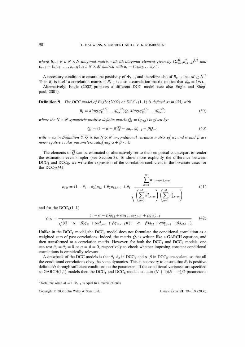
where Bt�1 is a NðN diagonal matrix with ith diagonal element given by �MhD1u2i,t�h�

1/2 andLt�1 D �ut�1, . . . , ut�M� is a NðM matrix, with ut D �u1tu2t . . . uNt�0.

A necessary condition to ensure the positivity of t�1, and therefore also of Rt, is that M ½ N.9

Then Rt is itself a correlation matrix if Rt�1 is also a correlation matrix (notice that �iit D 18i).Alternatively, Engle (2002) proposes a different DCC model (see also Engle and Shep-

pard, 2001).

Definition 9 The DCC model of Engle (2002) or DCCE�1, 1� is defined as in (35) with

Rt D diag�q�1/211,t . . . q

�1/2NN,t �Qt diag�q

�1/211,t . . . q

�1/2NN,t � �39�

where the NðN symmetric positive definite matrix Qt D �qij,t� is given by:

Qt D �1 � ˛� ˇ�QC ˛ut�1u0t�1 C ˇQt�1 �40�

with ut as in Definition 8. Q is the NðN unconditional variance matrix of ut, and ˛ and ˇ arenon-negative scalar parameters satisfying ˛C ˇ < 1.

The elements of Q can be estimated or alternatively set to their empirical counterpart to renderthe estimation even simpler (see Section 3). To show more explicitly the difference betweenDCCT and DCCE, we write the expression of the correlation coefficient in the bivariate case: forthe DCCT�M�

�12t D �1 � �1 � �2��12 C �2�12,t�1 C �1

M∑mD1

u1,t�mu2,t�m√√√√(

M∑mD1

u21,t�m

) (M∑mD1

u22,t�m

) �41�

and for the DCCE�1, 1�

�12t D �1 � ˛� ˇ�q12 C ˛u1,t�1u2,t�1 C ˇq12,t�1√��1 � ˛� ˇ�q11 C ˛u2

1,t�1 C ˇq11,t�1��1 � ˛� ˇ�q22 C ˛u22,t�1 C ˇq22,t�1�

�42�

Unlike in the DCCT model, the DCCE model does not formulate the conditional correlation as aweighted sum of past correlations. Indeed, the matrix Qt is written like a GARCH equation, andthen transformed to a correlation matrix. However, for both the DCCT and DCCE models, onecan test �1 D �2 D 0 or ˛ D ˇ D 0, respectively to check whether imposing constant conditionalcorrelations is empirically relevant.

A drawback of the DCC models is that �1, �2 in DCCT and ˛, ˇ in DCCE are scalars, so that allthe conditional correlations obey the same dynamics. This is necessary to ensure that Rt is positivedefinite 8t through sufficient conditions on the parameters. If the conditional variances are specifiedas GARCH(1,1) models then the DCCT and DCCE models contain �NC 1��NC 4�/2 parameters.

9 Note that when M D 1, t�1 is equal to a matrix of ones.



Interestingly, DCC models can be estimated consistently in two steps (see Section 3.2), whichmakes this approach feasible when N is high. Of course, when N is large, the restriction of commondynamics gets tighter, but for large N the problem of maintaining tractability also gets harder.In this respect, several variants of the DCC model are proposed in the literature. For example,Billio et al. (2003) argue that constraining the dynamics of the conditional correlation matrix tobe the same for all the correlations is not desirable. To solve this problem, they propose a block-diagonal structure where the dynamics is constrained to be identical only within each block. Theprice to pay for this additional flexibility is that the block members have to be defined a priori,which may be cumbersome in some applications. Pelletier (2003) proposes a model where theconditional correlations follow a switching regime driven by an unobserved Markov chain so thatthe correlation matrix is constant in each regime but may vary across regimes. Another extensionproposed by Engle (2002) consists of changing (40) into

Qt D Qþ �ii0 � A� B�C Aþ ut�1u0t�1 C Bþ Qt�1 �43�

where i is a vector of ones and A and B are NðN matrices of parameters. This increases thenumber of parameters considerably, but the matrices A and B could be defined to depend on asmall number of parameters (e.g. A D aa0).

To conclude, DCC models open the door to using flexible GARCH specifications in the variancepart. Indeed, as the conditional variances (together with the conditional means) can be estimatedusing N univariate models, one can easily extend the DCC-GARCH models to more complexGARCH-type structures (as mentioned at the beginning of Section 2.2). One can also extend thebivariate CCC FIGARCH model of Brunetti and Gilbert (2000) to a model of the DCC family.

General Dynamic Covariance ModelA model somewhat different from the previous ones but that nests several of them is the generaldynamic covariance (GDC) model proposed by Kroner and Ng (1998). They illustrate that thechoice of a multivariate volatility model can lead to substantially different conclusions in anapplication that involves forecasting dynamic variance matrices. We extend the definition of Kronerand Ng (1998) to cover models with dynamic conditional correlations.

Definition 10 The GDC model is defined as:

Ht D DtRtDt Cþt �44�

where

Dt D �dijt�, diit D√�iit 8i, dijt D 0 8i 6D j

t D ��ijt�

Rt is specified as DCCT�M�, see �36� and �37�, or as DCCE�1, 1�, see �39� and �40�

D ��ij�, �ii D 0 8i, �ij D �ji

�ijt D ωij C a0iεt�1ε

0t�1aj C g0

iHt�1gj 8i, j �45�

ai, gi, i D 1, . . . , N are �Nð 1� vectors of parameters, and D �ωij� is positive definite

and symmetric.



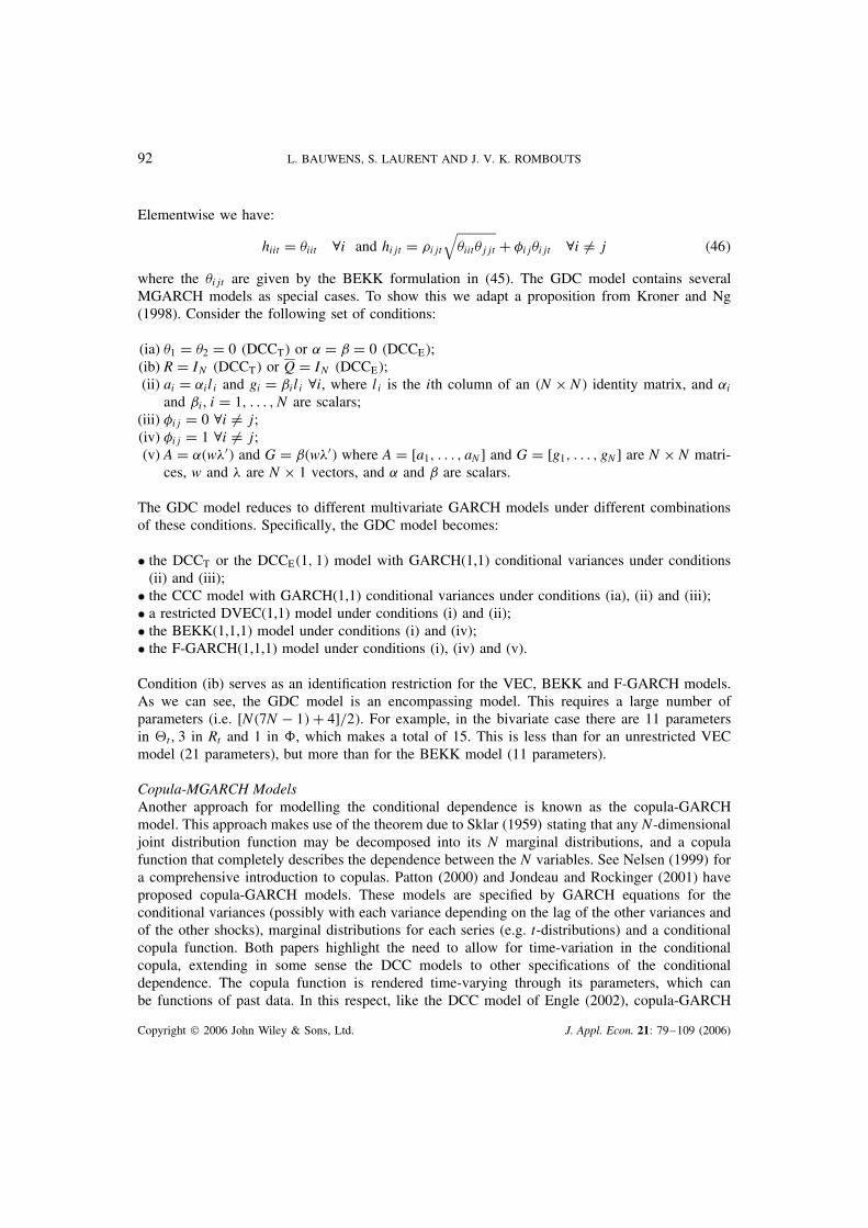
Elementwise we have:

hiit D �iit 8i and hijt D �ijt√�iit�jjt C �ij�ijt 8i 6D j �46�

where the �ijt are given by the BEKK formulation in (45). The GDC model contains severalMGARCH models as special cases. To show this we adapt a proposition from Kroner and Ng(1998). Consider the following set of conditions:

(ia) �1 D �2 D 0 �DCCT� or ˛ D ˇ D 0 �DCCE�;(ib) R D IN �DCCT� or Q D IN �DCCE�;(ii) ai D ˛ili and gi D ˇili 8i, where li is the ith column of an �NðN� identity matrix, and ˛i

and ˇi, i D 1, . . . , N are scalars;(iii) �ij D 0 8i 6D j;(iv) �ij D 1 8i 6D j;(v) A D ˛�w�0� and G D ˇ�w�0� where A D [a1, . . . , aN] and G D [g1, . . . , gN] are NðN matri-

ces, w and � are Nð 1 vectors, and ˛ and ˇ are scalars.

The GDC model reduces to different multivariate GARCH models under different combinationsof these conditions. Specifically, the GDC model becomes:

ž the DCCT or the DCCE�1, 1� model with GARCH(1,1) conditional variances under conditions(ii) and (iii);

ž the CCC model with GARCH(1,1) conditional variances under conditions (ia), (ii) and (iii);ž a restricted DVEC(1,1) model under conditions (i) and (ii);ž the BEKK(1,1,1) model under conditions (i) and (iv);ž the F-GARCH(1,1,1) model under conditions (i), (iv) and (v).

Condition (ib) serves as an identification restriction for the VEC, BEKK and F-GARCH models.As we can see, the GDC model is an encompassing model. This requires a large number ofparameters (i.e. [N�7N� 1�C 4]/2�. For example, in the bivariate case there are 11 parametersin t, 3 in Rt and 1 in , which makes a total of 15. This is less than for an unrestricted VECmodel (21 parameters), but more than for the BEKK model (11 parameters).

Copula-MGARCH ModelsAnother approach for modelling the conditional dependence is known as the copula-GARCHmodel. This approach makes use of the theorem due to Sklar (1959) stating that any N-dimensionaljoint distribution function may be decomposed into its N marginal distributions, and a copulafunction that completely describes the dependence between the N variables. See Nelsen (1999) fora comprehensive introduction to copulas. Patton (2000) and Jondeau and Rockinger (2001) haveproposed copula-GARCH models. These models are specified by GARCH equations for theconditional variances (possibly with each variance depending on the lag of the other variances andof the other shocks), marginal distributions for each series (e.g. t-distributions) and a conditionalcopula function. Both papers highlight the need to allow for time-variation in the conditionalcopula, extending in some sense the DCC models to other specifications of the conditionaldependence. The copula function is rendered time-varying through its parameters, which canbe functions of past data. In this respect, like the DCC model of Engle (2002), copula-GARCH



models can be estimated using a two-step maximum likelihood approach (see Section 3.2) whichsolves the dimensionality problem. An interesting feature of copula-GARCH models is the easewith which very flexible joint distributions may be obtained in the bivariate case. Their applicationto higher dimensions is a subject for further research.

2.4. Leverage Effects in MGARCH Models

For stock returns, negative shocks may have a larger impact on their volatility than positive shocksof the same absolute value (this is most often interpreted as the leverage effect unveiled by Black,1976). In other words, the news impact curve, which traces the relation between volatility andthe previous shock, is asymmetric. Univariate models that allow for this effect are the EGARCHmodel of Nelson (1991), the GJR model of Glosten et al. (1993) and the threshold ARCH modelof Zakoian (1994), among others. For multivariate series the same argument applies: the variancesand covariances may react differently to a positive than to a negative shock. In the multivariatecase, a shock can be defined in terms of εt or zt. Note that the signs of εit and zit do not necessarilycoincide, see (2).10

The MGARCH models reviewed in the previous subsections define the conditional variancematrix as a function of lagged values of εtε0

t. For example, each conditional variance in the VECmodel is a function of its own squared error but it is also a function of the squared errors of theother series as well as the cross-products of errors. A model that takes explicitly the sign of theerrors into account is the asymmetric dynamic covariance (ADC) model of Kroner and Ng (1998).The only difference with Definition 10 is an extra term based on the vector vt D max[0,�εt] in�ijt to take into account the sign of εit:

�ijt D ωij C a0iεt�1ε

0t�1aj C g0

iHt�1gj C b0ivt�1v

0t�1bj �47�

The ADC model nests some natural extensions of MGARCH models that incorporate the leverageeffect. Kroner and Ng (1998) apply the model to large and small firm returns. They find thatbad news about large firms can cause additional volatility in both small-firm and large-firmreturns. Furthermore, this bad news increases the conditional covariance. Small firm news hasonly minimal effects.

Hansson and Hordahl (1998) add the term Dþ vt�1v0t�1, in a DVEC model like (8), where D is

a diagonal matrix of parameters. To incorporate the leverage effect in the (bivariate) BEKK model,Hafner and Herwartz (1998) add the terms D0

1εt�1ε0t�1D1Dfε1,t�1< 0g C 10

2εt�1ε0t�1D21fε2,t�1< 0g, where

D1 and D2 are 2 ð 2 matrices of parameters and 1f...g is the indicator function. This generalizesthe univariate GJR specification.

2.5. Transformations of MGARCH Models

Not all MGARCH models are invariant with respect to linear transformations. By invariance ofa model, we mean that it stays in the same class if a linear transformation is applied to yt, sayQyt D Fyt, where F is a matrix of constants (for simplicity we assume F is square). If yt is a vectorof returns, a linear transformation corresponds to new assets (portfolios combining the originalassets). It seems sensible that a model should be invariant, otherwise the question arises which

10 Remember that H�1/2t and hence zt is not unique.



basic assets should be modelled. In some cases (stocks), these are naturally defined, in other cases,like exchange rates, they are not, since a reference currency must be chosen (see Gourieroux andJasiak, 2001, p. 140). Lack of invariance of a model does not imply that the model is not suitableat all for use in empirical work. Implications of invariance, or lack of invariance, are an openissue. For example, if the model is invariant, one can estimate it with some number of basic assets,as well as with a smaller number of portfolios of the basic assets. Estimates of the larger modelimply estimates of the smaller models, which could be compared to the direct estimates of thelatter. Very different estimates may lead us to question the specification.

Lack of invariance occurs whenever a diagonal matrix in the equation defining Ht is premul-tiplied by the matrix F defined above. The general VEC and BEKK models are invariant, buttheir diagonal versions are not. Conditional correlation models are not invariant, since FDt is notdiagonal when Dt is diagonal, see (31).

A related question is the marginalization of MGARCH processes: starting from a strongMGARCH model for yt, can we characterize the implied marginal process of a subvector ofyt, in particular of the scalar yit? Nijman and Sentana (1996) provide an answer to that question.11

To take a simple case, for a bivariate VEC(1,1) model, the implied process for y1t is at mosta weak GARCH (3,3) process.12 In the DVEC(1,1) case, the marginal process of y1t remainsa strong GARCH process. In proving such results, they use the VARMA(1,1) representation ofthe VEC(1,1) model ht D cC A�t�1 CGht�1, given by �t D c C �ACG��t�1 C ωt �Gωt�1 whereωt D �t � Et�1��t� is a martingale difference. Hence it is clear that this approach cannot be appliedto the conditional correlation models and the GDC model. Marginalization results for the lattermodels are not known.

Another question is that of temporal aggregation of MGARCH processes. Hafner (2004)shows that, like Drost and Nijman (1993) in the univariate case, the class of weak multivariateGARCH processes is closed under temporal aggregation. Weak multivariate GARCH models arecharacterized by a weak VARMA structure of �t in (7). Fourth moment characteristics turn outto be crucial for deriving the low-frequency dynamics. The issue of estimation of the parametersof the low-frequency model is difficult because the probability law of the innovation vector isunknown, since it is only assumed to be a weak white noise. See Hafner and Rombouts (2003)for more details.

2.6. Alternative Approaches to Multivariate Volatility

There are at least two other approaches to multivariate volatility than MGARCH models: stochasticvolatility (SV) models and realized volatility.

Multivariate stochastic volatility models (see e.g. Harvey et al., 1994) specify that the con-ditional variance matrix depends on some unobserved or latent processes rather than on pastobservations. A multivariate SV model is typically specified as N univariate SV models for theconditional variances (see Ghysels et al., 1996, for a survey of SV models):

εit D izit exp�0.5 hit� i D 1, . . . , N, t D 1, . . . , T �48�

11 Nijman and Sentana (1996) and Meddahi and Renault (1996) study the issue of contemporaneous aggregation, i.e., theaggregation of independent univariate GARCH processes.12 In a weak GARCH process, the dynamic equation for ht defines the best linear predictor of ε2

t given the past of εt. Ina strong GARCH, ht is the conditional variance. See Drost and Nijman (1993).



where i is a parameter. The innovation vector zt D �z1t, . . . , zNt�0 has E�zt� D 0 and Var�zt� D z,while the vector of volatilities ht D �h1t, . . . , hNt�0 follows a VAR(1) process ht D ht�1 C �twhere �t is i.i.d. ¾N�0, ��. In this model, the dynamics of the covariances depends onthe dynamics of the corresponding conditional variances, in other words, there is no directspecification of changing covariances or correlations. A drawback of SV models is the complexityof estimation.

Because the main emphasis of this survey is on ‘data-driven’ MGARCH models, a thor-ough discussion of the vast literature on latent factor models is beyond the scope of thispaper. The factor model in (21) becomes a latent model if Ft is latent, which means thatit is not included in It, implying that the conditional variance matrix, see for example (19),is not measurable any more. This is in contrast with Section 2.1, where the conditional vari-ance of the factors is specified as a function of the past data �εt�. Therefore, latent factormodels can be classified as stochastic volatility models as mentioned in Shephard (1996).The elements of Ft typically follow dynamic heteroscedastic processes, for example Dieboldand Nerlove (1989) use ARCH models. The fact that the factor is considered as nonobserv-able complicates inference considerably, since the likelihood function must be marginalizedwith respect to it (see Gourieroux, 1997, section 6.3). The conditional covariance betweenthe factors is usually assumed to be equal to zero. See Sentana and Fiorentini (2001) andFiorentini et al. (2004) for more details on identification and estimation of factor models. Sen-tana (1998) shows that the observed factor model is observationally equivalent (up to con-ditional second moments) to a class of conditionally heteroscedastic factor models includinglatent factor models. Doz and Renault (2003) elaborate on this result and draw the conclu-sions in terms of model specification and identification, and in terms of inference methodolo-gies.

The second alternative has been proposed by Andersen et al. (2003). In this case, a dailymeasure of variances and covariances is computed as an aggregate measure from intradayreturns. More specifically, a daily realized variance for day t is computed as the sum of thesquared intraday equidistant returns for the given trading day and a daily realized covarianceis obtained by summing the products of intraday returns. Once such daily measures havebeen obtained, they can be modelled, e.g. for a prediction purpose. A nice feature of thisapproach is that unlike MGARCH and multivariate stochastic volatility models, the N�N� 1�/2covariance components of the conditional variance matrix (or, rather, the components of itsCholeski decomposition) can be forecasted independently, using as many univariate models. Asshown by Andersen et al. (2003), although the use of the realized covariance matrix facilitatesrigorous measurement of conditional volatility in much higher dimensions than is feasible withMGARCH and multivariate SV models, it does not allow the dimensionality to become arbitrarilylarge. Indeed, to ensure the positive definiteness of the realized covariance matrix, the numberof assets (N) cannot exceed the number of intraday returns for each trading day. The maindrawback is that intraday data remain relatively costly and are not readily available for allassets. Furthermore, a large amount of data handling and computer programming is usuallyneeded to retrieve the intraday returns from the raw data files supplied by the exchanges ordata vendors. On the contrary, working with daily data is relatively simple and the data arebroadly available.

Which approach is best, for example in terms of forecasting, is beyond the scope of the paperand an interesting topic for future theoretical and empirical research.



3. ESTIMATION

In the previous section we have defined existing specifications of conditional variance matricesthat enter the definition either of a data generating process (DGP) or of a model to be estimated. InSection 3.1 we discuss maximum likelihood (ML) estimation of these models, and in Section 3.2we explain a two-step approach for estimating conditional correlation models. Finally, we reviewbriefly various issues related to practical estimation in Section 3.3.

3.1. Maximum Likelihood

Suppose the vector stochastic process fytg (for t D 1, . . . , T) is a realization of a DGP whose condi-tional mean, conditional variance matrix and conditional distribution are respectively �t��0�,Ht��0�and p�ytj�0, It�1�, where �0 D ��0 �0� is a r-dimensional parameter vector and �0 is the vector thatcontains the parameters of the distribution of the innovations zt (there may be no such parameter).Importantly, to justify the choice of the estimation procedure, we assume that the model to beestimated encompasses the true formulations of �t��0� and Ht��0�.

The procedure most often used in estimating �0 involves the maximization of a likelihoodfunction constructed under the auxiliary assumption of an i.i.d. distribution for the standardizedinnovations zt. The i.i.d. assumption may be replaced by the weaker assumption that zt is amartingale difference sequence with respect to It�1, but this type of assumption does not translateinto the likelihood function. The likelihood function for the i.i.d. case can then be viewed as aquasi-likelihood function.

Consequently, one has to make an additional assumption on the innovation process by choosinga density function, denoted g�zt��j��, where � is a vector of nuisance parameters. The problemto solve is thus to maximize the sample loglikelihood function LT��, �� for the T observations(conditional on some starting values for �0 and H0), with respect to the vector of parameters� D ��, ��, where

LT�� DT∑tD1

logf�ytj�, It�1� �49�

withf�ytj�, It�1� D jHtj�1/2g�H�1/2

t �yt � �t�j�� 50�

and the dependence with respect to � occurs through �t and Ht. The term jHtj�1/2 is the Jacobianthat arises in the transformation from the innovations to the observables. Note that unless g�Ð�belongs to the class of elliptical distributions, i.e. is a function of z0tzt, the ML estimator dependson the choice of decomposition of H1/2

t , since z0tzt D �yt � �t�0H�1t �yt � �t�.

The most commonly employed distribution in the literature is the multivariate normal, uniquelydetermined by its first two moments (so that � D � since � is empty). In this case, the sampleloglikelihood is (up to a constant):

LT�� D �1

2

T∑tD1

log jHtj � 1

2

T∑tD1

�yt � �t�0H�1

t �yt � �t� �51�

It is well known that the normality of the innovations is rejected in most applications dealingwith daily or weekly data. In particular, the kurtosis of most financial asset returns is larger than



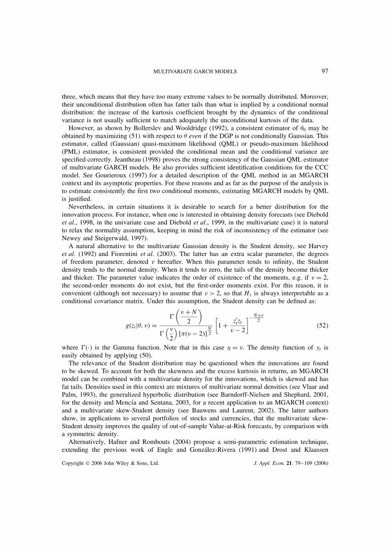
three, which means that they have too many extreme values to be normally distributed. Moreover,their unconditional distribution often has fatter tails than what is implied by a conditional normaldistribution: the increase of the kurtosis coefficient brought by the dynamics of the conditionalvariance is not usually sufficient to match adequately the unconditional kurtosis of the data.

However, as shown by Bollerslev and Wooldridge (1992), a consistent estimator of �0 may beobtained by maximizing (51) with respect to � even if the DGP is not conditionally Gaussian. Thisestimator, called (Gaussian) quasi-maximum likelihood (QML) or pseudo-maximum likelihood(PML) estimator, is consistent provided the conditional mean and the conditional variance arespecified correctly. Jeantheau (1998) proves the strong consistency of the Gaussian QML estimatorof multivariate GARCH models. He also provides sufficient identification conditions for the CCCmodel. See Gourieroux (1997) for a detailed description of the QML method in an MGARCHcontext and its asymptotic properties. For these reasons and as far as the purpose of the analysis isto estimate consistently the first two conditional moments, estimating MGARCH models by QMLis justified.

Nevertheless, in certain situations it is desirable to search for a better distribution for theinnovation process. For instance, when one is interested in obtaining density forecasts (see Dieboldet al., 1998, in the univariate case and Diebold et al., 1999, in the multivariate case) it is naturalto relax the normality assumption, keeping in mind the risk of inconsistency of the estimator (seeNewey and Steigerwald, 1997).

A natural alternative to the multivariate Gaussian density is the Student density, see Harveyet al. (1992) and Fiorentini et al. (2003). The latter has an extra scalar parameter, the degreesof freedom parameter, denoted � hereafter. When this parameter tends to infinity, the Studentdensity tends to the normal density. When it tends to zero, the tails of the density become thickerand thicker. The parameter value indicates the order of existence of the moments, e.g. if � D 2,the second-order moments do not exist, but the first-order moments exist. For this reason, it isconvenient (although not necessary) to assume that � > 2, so that Ht is always interpretable as aconditional covariance matrix. Under this assumption, the Student density can be defined as:

g�ztj�, �� D

(� CN

2

)

(�

2

)[�� 2�]

N2

[1 C z0tzt

� � 2

]�NC�2

�52�

where �Ð� is the Gamma function. Note that in this case � D �. The density function of yt iseasily obtained by applying (50).

The relevance of the Student distribution may be questioned when the innovations are foundto be skewed. To account for both the skewness and the excess kurtosis in returns, an MGARCHmodel can be combined with a multivariate density for the innovations, which is skewed and hasfat tails. Densities used in this context are mixtures of multivariate normal densities (see Vlaar andPalm, 1993), the generalized hyperbolic distribution (see Barndorff-Nielsen and Shephard, 2001,for the density and Mencıa and Sentana, 2003, for a recent application to an MGARCH context)and a multivariate skew-Student density (see Bauwens and Laurent, 2002). The latter authorsshow, in applications to several portfolios of stocks and currencies, that the multivariate skew-Student density improves the quality of out-of-sample Value-at-Risk forecasts, by comparison witha symmetric density.

Alternatively, Hafner and Rombouts (2004) propose a semi-parametric estimation technique,extending the previous work of Engle and Gonzalez-Rivera (1991) and Drost and Klaassen



(1997) to MGARCH models. This consists of first estimating the model by QML, which providesconsistent estimates of the innovations. In a second step, these are used to estimate the functiong�Ð� nonparametrically. Finally, the parameters of the GARCH model are estimated using Og�Ð� todefine the likelihood function.

The asymptotic properties of ML and QML estimators in multivariate GARCH models arenot yet firmly established, and are difficult to derive from low level assumptions. As mentionedpreviously, consistency has been shown by Jeantheau (1998). Asymptotic normality of the QMLEis not established generally. Gourieroux (1997, section 6.3) proves it for a general formulationusing high level assumptions. Comte and Lieberman (2003) prove it for the BEKK formulation.Since F-GARCH and (G)O-GARCH models are special cases of the BEKK model, this result holdsalso for these two models (see van der Weide, 2002). Researchers who use MGARCH modelshave generally proceeded as if asymptotic normality holds in all cases. Asymptotic normality ofthe MLE and QMLE has been proved in the univariate case under low level assumptions, one ofwhich is the existence of moments of order four or higher of the innovations (see Lee and Hansen,1994; Lumsdaine, 1996; Ling and McAleer, 2003). However, Hall and Yao (2003) show that theasymptotic distribution of the QMLE in the univariate GARCH(p, q) model is not normal, but isa multivariate stable distribution (with fatter tails than the normal) if the innovations are in thedomain of attraction of a stable law with exponent smaller than two (implying nonexisting fourthmoments). Extension of this result to the multivariate case is a subject for further research.

Finally, it is worth mentioning that the conditional mean parameters may be consistentlyestimated in a first stage, prior to the estimation of the conditional variance parameters, forexample for a VARMA model, but not for a GARCH-in-mean model. Estimating the parameterssimultaneously with the conditional variance parameters would increase the efficiency at leastin large samples (unless the asymptotic covariance matrix is block diagonal between the meanand variance parameters), but this is computationally more difficult. For this reason, one usuallytakes either a very simple model for the conditional mean or one considers yt � O�t as the datafor fitting the MGARCH model. A detailed investigation of the consequences of such a two-stepprocedure on properties of estimators has still to be conducted. Conditions for block diagonalityof the asymptotic covariance matrix have also to be worked out (generalizing results of Engle,1982 for the univariate case).

3.2. Two-Step Estimation

A useful feature of the DCC models presented earlier is that they can be estimated consistentlyusing a two-step approach. Engle and Sheppard (2001) show that in the case of a DCCE model,the loglikelihood can be written as the sum of a mean and volatility part (depending on a set ofunknown parameters �Ł

1) and a correlation part (depending on �Ł2).

Indeed, recalling that the conditional variance matrix of a DCC model can be expressed asHt D DtRtDt, an inefficient but consistent estimator of the parameter �Ł

1 can be found by replacingRt by the identity matrix in (51). In this case the quasi-loglikelihood function corresponds to thesum of loglikelihood functions of N univariate models:

QL1T��Ł1� D �1

2

T∑tD1

N∑iD1

[log�hiit�C �yit � �it�

2

hiit

]�53�



Given �Ł1 and under appropriate regularity conditions, a consistent, but inefficient, estimator of �Ł

2can be obtained by maximizing:

QL2T��Ł2 j�Ł

1� D �1

2

T∑tD1

�log jRtj C u0tR

�1t ut� �54�

where ut D D�1t �yt � �t�. The sum of the likelihood functions in (53) and (54), plus half of the

total sum of squared standardized residuals (∑

t u0tut/2, which is almost equal to NT /2), is equal to

the loglikelihood in (51). It is thus possible to compare the loglikelihood of the two-step approachwith that of the one-step approach and of other models.

Engle and Sheppard (2001) explain that the estimators O�Ł1 and O�Ł

2 , obtained by maximizing(53) and (54) separately, are not fully efficient (even if zt is normally distributed) since they arelimited information estimators. However, one iteration of a Newton–Raphson algorithm applied tothe total likelihood (51), starting at �O�Ł

1 , O�Ł2�, provides an estimator that is asymptotically efficient.

Another two-step approach for the diagonal VEC model is proposed by Ledoit et al. (2003). Toavoid estimating c, A and G jointly, they estimate each variance and covariance equation separately.The resulting estimates do not necessarily guarantee positive semi-definite Ht’s. Therefore, ina second step, the estimates are transformed in order to achieve the requirement, keeping thedisruptive effects as small as possible. The transformed estimates are still consistent with respectto the parameters of the DVEC model.

3.3. Various Issues

Analytical vs. Numerical ScoreTypically, for conditionally heteroscedastic models, numerical techniques are used to approximatethe derivatives of the loglikelihood function (the score) with respect to the parameter vector. Asshown by Fiorentini et al. (1996) and McCullough and Vinod (1999), in a univariate framework,using analytical scores in the estimation procedure improves the numerical accuracy of the resultingestimates and speeds-up ML estimation. According to Hafner and Rombouts (2004), the scorevector corresponding to a term of (49) takes the form

st�� D ∂vec�Ht�0

∂�

{�1

2vec�H�1

t �� DNDCN�IN �Ht CH1/2

t �H1/2t ��1vec

(∂ log g�zt�

∂ztz0t

)}�55�

where st�� D ∂ logf�ytj�, It�1�/∂�, vec�Ð� is the operator that stacks the columns of a MðNmatrix into a MNð 1 vector, DN is the duplication matrix defined so that DNvech�A� D vec�A�for every symmetric matrix A of order N and DC

N is its generalized inverse. As pointed out by areferee, one sees from (55) that the choice of the square root matrix H1/2

t has consequences forthe exact form of the score.

In this respect, Lucchetti (2002) proposes a closed-form expression of the score vector for theBEKK model with a Gaussian loglikelihood. Hafner and Herwartz (2003) also provide analyticalformulae for the score and the Hessian of a general MGARCH model in a QML framework andpropose two methods to estimate the expectation of the Hessian. The authors show in a simulationstudy that analytical derivatives clearly outperform numerical methods.



Variance TargetingWe have seen that what renders most MGARCH models difficult for estimation is their high numberof parameters. A simple trick to ensure a reasonable value of the model-implied unconditionalcovariance matrix, which also helps to reduce the number of parameters in the maximization ofthe likelihood function, is referred to as variance targeting by Engle and Mezrich (1996). Forexample, in the VEC model (and all its particular cases), the conditional variance matrix may beexpressed in terms of the unconditional variance matrix (see earlier) and other parameters. Doingso one can reparametrize the model using the unconditional variance matrix and replace it by aconsistent estimator (before maximizing the likelihood). When doing this, one should correct thecovariance matrix of the estimator of the other parameters for the uncertainty in the preliminaryestimator. In DCC models, this can also be done with the constant matrix of the correlation part,e.g. Q in (40). In this case, the two-step estimation procedure explained in Section 3.2 becomes athree-step procedure.

Imposing or Not the Positivity ContraintsA key problem in MGARCH models is that the conditional variance matrix has to be positivedefinite almost surely for all t. As shown in the previous section this is done by constraining theparameter space (for instance by using a constrained optimization algorithm), assuming that theconstraints are known. However, these constraints are usually sufficient but not necessary. Forinstance, we know since Nelson and Cao (1992) that imposing ωi > 0 and ˛i, ˇi ½ 0 in (34) isoverly restrictive and that negative values of ˛i and ˇi are not incompatible with a positiveconditional variance. If one imposes positivity restrictions to facilitate estimation, one incurs therisk of rejecting �0 from the parameter space.

SoftwareBrooks et al. (2003) review the relatively small number of software packages that are currentlyavailable for estimating MGARCH models. It is obvious that the development of MGARCHmodels in standard econometric packages is still in its infancy, and that further developmentswould greatly help applied researchers who cannot afford to program the estimation of a particularmodel, but who would rather try several models and distributions.

4. DIAGNOSTIC CHECKING

Since estimating MGARCH models is time-consuming, both in terms of computations and theirprogramming (if needed), it is desirable to check ex ante whether the data present evidence ofmultivariate ARCH effects. Ex post, it is also of crucial importance to check the adequacy ofthe MGARCH specification. However, compared to the huge body of diagnostic tests devoted tounivariate models, few tests are specific to multivariate models.

In the current literature on MGARCH models, one can distinguish two kinds of specificationtests, namely univariate tests applied independently to each series and multivariate tests applied tothe vector series as a whole. We deliberately leave out the first kind of tests and refer interestedreaders to surveys of univariate ARCH processes (see Section 1). As emphasized by Kroner andNg (1998), the existing literature on multivariate diagnostics is sparse compared to the univariatecase. However, although univariate tests can provide some guidance, contemporaneous correlationof disturbances entails that statistics from individual equations are not independent. As a result,



combining test decisions over all equations raises size control problems, so the need for jointtesting naturally arises (Dufour et al., 2003).

Since the dynamics of the series is assumed to be captured by the model (at least in the firsttwo conditional moments), the standardized error term zt D H�1/2

t εt should obey the followingmoment conditions (see Ding and Engle, 2001):13

(A) E�ztz0t� D IN(B) Cov�z2

it, z2jt� D 0, for alli 6D j

(C) Cov�z2it, z

2j,t�k� D 0, fork > 0

While testing A has power to detect misspecification in the conditional mean, testing B is suitedto check if the conditional distribution is Gaussian, which could be false even if Ht is correctlyspecified. In contrast, testing C aims at checking the adequacy of the dynamic specification ofHt, regardless of the validity of the assumption about the distribution of zt. Ding and Engle(2001) show that if the true conditional distribution is the multivariate Student described in (52),Cov�z2

it, z2jt� D 2�2/[�� 4�� 2�2], for i 6D j, which is different from 0 when 1/� 6D 0 (the none-

Gaussian case). Moreover, starting from a conditionally homoscedastic multivariate regressionmodel (i.e. Ht D H, 8t), testing C is equivalent to testing the presence of ARCH effects in thedata. Provided that a sufficient number of moments exist (which is not always the case), testingconditions A–C could be done using the conditional moment test principle of Newey (1985) andTauchen (1985).

A quite different approach aims at checking the overall adequacy of a model, i.e. the coincidenceof the assumed density f�ytj�, �, It�1� and the true density p�ytj�0, �0, It�1��8t�. Diebold et al.(1998) (in the univariate case) and Diebold et al. (1999) (in the multivariate case) propose anelegant and practical procedure based on the concept of density forecasts. For more details aboutdensity forecasts and their applications in finance, see the special issue of the Journal of Forecasting(Timmermann, 2000).

As mentioned by Tse (2002), diagnostics for conditional heteroscedasticity models applied inthe literature can be divided into three categories: portmanteau tests of the Box–Pierce–Ljungtype, residual-based diagnostics and Lagrange multiplier tests.

4.1. Portmanteau Statistics

The most widely used diagnostics to detect ARCH effects are probably the Box–Pierce/Ljung–Boxportmanteau tests. Following Hosking (1980), a multivariate version of the Ljung–Box test statisticis given by:

HM�M� D T2M∑jD1

�T� j��1trfC�1Yt �0�CYt �j�C

�1Yt �0�C

0Yt �j�g �56�

where Yt D vech�yty0t� and CYt�j� is the sample autocovariance matrix of order j. Under the null

hypothesis of no ARCH effects, HM (M) is distributed asymptotically as �2�K2M�. Duchesne andLalancette (2003) generalize this statistic using a spectral approach and obtain higher asymptotic

13 The definition of the exact form of the square root matrix H1/2t is deliberately left unspecified by Ding and Engle

(2001). It is not known to what extent a particular choice has a consequence on the tests presented in this section.



power by using a different kernel than the truncated uniform kernel used in HM (M). This testis also used to detect misspecification in the conditional variance matrix Ht, by replacing yt byOzt D OH�1/2

t Oεt. The asymptotic distribution of the portmanteau statistics is, however, unknown inthis case since Ozt has been estimated. Furthermore, ad hoc adjustments of degrees of freedom for thenumber of estimated parameters have no theoretical justification. In such a case, portmanteau testsshould be interpreted with care even if simulation results reported by Tse and Tsui (1999) suggestthat they provide a useful diagnostic in many situations.

Ling and Li (1997) propose an alternative portmanteau statistic for multivariate conditionalheteroscedasticity. They define the sample lag-h (transformed) residual autocorrelation as:

QR�h� D

T∑tDhC1

�Oε0tOH�1t Oεt �N��Oε0

t�h OH�1t�h Oεt�h �N�

T∑tDhC1

�Oε0tOH�1t Oεt �N�2

�57�

Their test statistic is given by LL�M� D T∑M

hD1QR2�h� and is asymptotically distributed as �2�M�

under the null of no conditional heteroscedasticity. In the derivation of the asymptotic results,normality of the innovation process is not assumed. The statistic is thus robust with regardto the distribution choice. Tse and Tsui (1999) show that there is a loss of information inthe transformation Oε0

tOH�1t Oεt of the residuals and the test may suffer from a power reduction.

Furthermore, Duchesne and Lalancette (2003) argue that if an inappropriate choice ofM is selected,the resulting test statistic may be quite inefficient (the same comment applies to the residual-basedtests presented below). For these reasons, these authors propose a more powerful version of theLL(M) test based on the spectral density of the stochastic process fε0

tH�1t εt, t 2 Zg, which is i.i.d.

under the null of homoscedasticity. Interestingly, since their test is based on a spectral densityestimator, a data-dependent choice of M is available.

4.2. Residual-Based Diagnostics

These tests involve running regressions of the cross-products of the standardized residuals � Out� onsome explanatory variables and testing for the statistical significance of the regression coefficients.The key problem is that since the regressors (transformed residuals) are obtained after estimating afirst model and so depend on estimated parameters with their own uncertainty, the usual OLS theorydoes not apply. The contribution of Tse (2002) is to establish the asymptotic distribution of the

OLS estimator in this context. Let us define Ouit D Oεit/√

Ohiit as the ith �i D 1, . . . , N� standardized

residual at time t and O�ijt D Ohijt/√

Ohiit Ohjjt as the estimated conditional correlation between yit andyjt. Tse (2002) proposes to run the following regressions:

Ou2it � 1 D Od0

itυi C �it, i D 1, . . . , N �58�

Ouit Oujt � O�ijt D Od0ijtυij C �ijt, 1 � i < j � N �59�

where Odit and Odiit are the estimated counterparts of respectively dit D �u2i,t�1, . . . , u

2i,t�M�

0, dijt D�ui,t�1uj,t�1, . . . , ui,t�Muj,t�M�0, and υi and υij are the regression coefficients. The choice of the



regressors may be changed depending on the particular type of model inadequacy one wants toinvestigate. An advantage of the residual-based diagnostics is that they focus on several distinctiveaspects of possible causes of ‘remaining’ ARCH effects.

Tse (2002) shows that under reasonable assumptions the statistics RB�M�1 D TOυ0iOLi O�1

iOLiOυi and

RB�M�2 D TOυ0ij

OLij O�1ij

OLijOυij are each asymptotically distributed as �2�M� under the null of correctspecification of the first two conditional moments, where

Li D plim(

1

T

∑ditd

0it

)Lij D plim

(1

T

∑dijtd

0ijt

)�60�

i D Ef�u2it � 1�2gLi � QiGQ

0i ij D Ef�uitujt � 1�2gLij � QijGQ

0ij �61�

Qi D plim

{1

T

∑dit∂u2it

∂�0

}Qij D plim

{1

T

∑dijt

∂�uitujt � �ijt�

∂�0

}�62�

and assuming that under certain conditions, the MLE estimate of � satisfies the conditionpT�O� � �� ! N�0, G�. Naturally, to compute these statistics, one has to replace the unobservable

components by their estimated counterparts.

4.3. Lagrange Multiplier Tests

Lagrange multiplier tests usually have a higher power than portmanteau tests when the alternativeis correct (although they can be asymptotically equivalent in certain cases), but they may havelow power against other alternatives. Bollerslev et al. (1988) and Engle and Kroner (1995),among others, have developed LM tests for MGARCH models. Recently, Sentana and Fiorentini(2001) have developed a simple preliminary test for ARCH effects in common factor models.

To reduce the number of parameters in the estimation of MGARCH models, it is usualto introduce restrictions. For instance, the CCC model of Bollerslev (1990) assumes that theconditional correlation matrix is constant over time. It is then desirable to test this assumptionafterwards. Tse (2000) proposes a test for constant correlations. The null is hijt D �ij

√hiithjjt

where the conditional variances are GARCH (1,1), the alternative is hijt D �ijt√hiithjjt. The

test statistic is a LM statistic which under the null is asymptotically �2�N�N� 1�/2�. Bera andKim (2002) also develop a test for constancy of the correlation parameters in the CCC model ofBollerslev (1990). It is an information matrix-type test that besides constant correlations examinesat the same time various features of the specified model. An alternative test has been proposed byLongin and Solnik (1995).

Engle and Sheppard (2001) propose another test of the constant correlation hypothesis, in thespirit of the DCC models presented earlier. The null H0 : Rt D R8t is tested against the alternativeH1 : vech�Rt� D vech�R�C ˇŁ

1vech�Rt�1�C Ð Ð Ð C ˇŁpvech�Rt�p�. The test is easy to implement

since H0 implies that coefficients in the regression Xt D ˇŁ0 C ˇŁ

1Xt�1 C Ð Ð Ð C ˇŁpXt�p C uŁ

t areequal to zero, where Xt D vechu�Ozt Oz0t � IN�, vechu is like the vech operator but it only selects the

elements under the main diagonal, Ozt D OR�1/2 OD�1t O2t is the Nð 1 vector of standardized residuals

(under the null), and Dt D diag�h1/211t . . . h

1/2NNt�.



5. CONCLUSION

The main purpose of this paper is to review MGARCH models. Since the seminal paper of Engle(1982), much progress has been made in understanding GARCH models and their multivariateextensions. As mentioned in Section 1, these models are increasingly used in applied financialeconometrics. Given the large and increasing variety of existing models, an applied econometricianis confronted with the issue of choosing among them for each particular application. A relatedquestion is ‘which model is most appropriate under which circumstances?’.

Applied research has naturally followed theoretical research and used existing models. Thereare very few papers where a comparison of different MGARCH models for the same problem anddata is done.14 The discussion paper version of this article—see Bauwens et al. (2003)—containsa detailed review of the application fields and gives an idea of which models have been used foreach field. This reveals that to a large extent, when a model came out in the literature, appliedresearchers soon started to try it, discarding the previous models. This partly reflects the fact thatparsimonious models were introduced progressively to overcome the difficulty of estimating theVEC model.

In our opinion, the crucial point in MGARCH modelling is to provide a realistic but parsimoniousspecification of the variance matrix ensuring its positivity. There is a dilemma between flexibilityand parsimony. BEKK models are flexible but require too many parameters for multiple time seriesof more than four elements. Diagonal VEC and BEKK models are much more parsimonious butvery restrictive for the cross-dynamics. They are not suitable if volatility transmission is theobject of interest, but they usually do a good job in representing the dynamics of variances andcovariances. This may be sufficient for some applications like asset pricing models.

In contrast, factor GARCH models allow the conditional variances and covariances to dependon the past of all variances and covariances, but they imply common persistence in all theseelements. In this respect, the DCC models allow for different persistence between variances andcorrelations, but impose common persistence in the latter (although this may be relaxed). Theyopen the door to handling more than a very small number of series. They are an extension of theCCC model which is relatively easy to estimate.

One way to deal with flexible but heavily parametrized models is to keep a flexible functionalform and to reduce the number of parameters by imposing restrictions. An example of this approachis provided in Engle et al. (1990a), who impose restrictions in a VEC model. We conjecture thatresearchers will propose new ways to impose restrictions. An idea is to base the restrictionson preliminary (easy to obtain) estimates, in the spirit of Ledoit et al. (2003) or Bauwens andRombouts (2003).

Finally, here is a list of open issues/research topics (stated in a condensed way since they havebeen discussed in this survey):

1. Improving software for inference (this is a prerequisite for progress in applications).2. Comparing the performance and assessing the financial value of different specifications in

applications.15

3. Implications of stability or not of a model class with respect to linear transformations.4. More flexible specifications for the dynamics of correlations of DCC models.

14 Examples are Karolyi (1995), Bera et al. (1997), Kroner and Ng (1998), Engle and Sheppard (2001).15 See Rombouts and Verbeek (2004) and Fleming et al. (2003) for recent examples.



5. Unconditional moments of correlations/covariances, marginalization and temporal aggregationin DCC models.

6. Development of a copula tool for specification and inference.7. Impact of choice of the square root decomposition of Ht on statistical procedures.8. Conditions for two-step efficient estimation (MGARCH on residuals of the mean model).9. Asymptotic properties of MLE (in particular low level, easy to check, sufficient conditions for

asymptotic normality when it holds).10. Further developments of multivariate diagnostic tests.

There is little doubt that progress on these issues would greatly contribute to the theory andpractice of MGARCH models.

ACKNOWLEDGEMENTS

The authors would like to thank Christian Hafner and Roy van der Weide for useful comments.They are especially grateful to three referees and the editor (T. Bollerslev) for their detailedcomments and numerous suggestions that helped to improve the paper. This text presents researchresults of the Belgian Programme on Interuniversity Poles of Attraction initiated by the BelgianState Prime Minister’s Office, Science Policy Programming. Scientific responsibility is assumedby the authors.

REFERENCES

Alexander CO. 2001. Market Models. John Wiley: New York.Alexander CO, Chibumba AM. 1997. Multivariate orthogonal factor GARCH. Mimeo, University of Sussex.Andersen TG, Bollerslev T, Diebold FX, Labys P. 2003. Modeling and forecasting realized volatility.

Econometrica 71: 579–625.Attanasio O. 1991. Risk, time-varying second moments and market efficiency. Review of Economic Studies

58: 479–494.Baillie RT, Bollerslev T, Mikkelsen HO. 1996. Fractionally integrated generalized autoregressive conditional

heteroskedasticity. Journal of Econometrics 74: 3–30.Barndorff-Nielsen OE, Shephard N. 2001. Normal modified stable processes. Theory of Probability and

Mathematics Statistics 65: 1–19.Bauwens L, Laurent S. 2002. A new class of multivariate skew densities, with application to GARCH models.

Journal of Business and Economic Statistics .Bauwens L, Rombouts JVK. 2003. Bayesian clustering of similar GARCH models. CORE DP 2003/87.Bauwens L, Laurent S, Rombouts JVK. 2003. Multivariate GARCH models: a survey. CORE DP 2003/31.Bera AK, Higgins ML. 1993. ARCH models: properties, estimation and testing. Journal of Economic Surveys

7: 305–362.Bera AK, Kim S. 2002. Testing constancy of correlation and other specifications of the BGARCH model

with an application to international equity returns. Journal of Empirical Finance 9: 171–195.Bera AK, Garcia P, Roh JS. 1997. Estimation of time-varying hedging ratios for corns and soybeans:

BGARCH and random coefficient approaches. Sankhya 59: 346–368.Billio M, Caporin M, Gobbo M. 2003. Block dynamic conditional correlation multivariate GARCH models.

Greta Working Paper 03.03.Black F. 1976. Studies of stock market volatility changes. Proceedings of the American Statistical Association,

Business and Economic Statistics Section, pp. 177–181.Bollerslev T. 1986. Generalized autoregressive conditional heteroskedasticity. Journal of Econometrics 31:

307–327.



Bollerslev T. 1990. Modeling the coherence in short-run nominal exchange rates: a multivariate generalizedARCH model. Review of Economics and Statistics 72: 498–505.

Bollerslev T, Chou RY, Kroner KF. 1992. ARCH modeling in finance: a review of the theory and empiricalevidence. Journal of Econometrics 52: 5–59.

Bollerslev T, Engle RF. 1993. Common persistence in conditional variances. Econometrica 61: 167–186.Bollerslev T, Engle RF, Nelson DB. 1994. ARCH models. In Handbook of Econometrics, Engle R, McFad-

den D (eds). North Holland Press: Amsterdam.Bollerslev T, Engle RF, Wooldridge JM. 1988. A capital asset pricing model with time varying covariances.

Journal of Political Economy 96: 116–131.Bollerslev T, Wooldridge JM. 1992. Quasi-maximum likelihood estimation and inference in dynamic models

with time-varying covariances. Econometric Reviews 11: 143–172.Box GEP, Jenkins GM. 1970. Time Series Analysis, Forecasting and Control. Holden-Day: San Francisco.Brooks C, Burke SP, Persand G. 2003. Multivariate GARCH models: software choice and estimation issues.

Journal of Applied Econometrics 18: 725–734.Brunetti C, Gilbert CL. 2000. Bivariate FIGARCH and fractional cointegration. Journal of Empirical Finance

7: 509–530.Christodoulakis GA, Satchell SE. 2002. Correlated ARCH: modelling the time-varying correlation between

financial asset returns. European Journal of Operations Research 139: 351–370.Comte F, Lieberman O. 2003. Asymptotic theory for multivariate GARCH processes. Journal of Multivariate

Analysis 84: 61–84.De Santis G, Gerard B. 1998. How big is the premium for currency risk? Journal of Financial Economics

49: 375–412.Diebold FX, Nerlove M. 1989. The dynamics of exchange rate volatility: a multivariate latent factor ARCH

model. Journal of Applied Econometrics 4: 1–21.Diebold FX, Gunther TA, Tay AS. 1998. Evaluating density forecasts, with applications to financial risk

management. International Economic Review 39: 863–883.Diebold FX, Hahn J, Tay AS. 1999. Multivariate density forecast evaluation and calibration in financial

risk management: high-frequency returns on foreign exchange. Review of Economics and Statistics 81:863–883.

Ding Z, Engle RF. 2001. Large scale conditional covariance matrix modeling, estimation and testing. WorkingPaper FIN-01-029, NYU Stern School of Business.

Ding Z, Granger CWJ, Engle RF. 1993. A long memory property of stock market returns and a new model.Journal of Empirical Finance 1: 83–106.

Doz C, Renault E. 2003. Conditionally heteroskedastic factor models: identification and instrumental vari-ables estimation. Mimeo.

Drost CD, Klaassen CAJ. 1997. Efficient estimation in semiparametric GARCH models. Journal of Econo-metrics 81: 193–221.

Drost CD, Nijman T. 1993. Temporal aggregation of GARCH processes. Econometrica 61: 909–927.Duchesne P, Lalancette S. 2003. On testing for multivariate ARCH effects in vector time series models. La

Revue Canadienne de Statistique 31: 275–292.Dufour J-M, Khalaf L, Beaulieu M-C. 2003. Finite-sample diagnostics for multivariate regression with

applications to linear asset pricing models. Working Paper No. 06-2003, CIREQ.El Babsiri M, Zakoian J-M. 2001. Contemporaneous asymmetry in GARCH processes. Journal of Econo-

metrics 101: 257–294.Engle R, Kroner FK. 1995. Multivariate simultaneous generalized ARCH. Econometric Theory 11: 122–150.Engle R, Mezrich J. 1996. GARCH for groups. RISK 9: 36–40.Engle RF. 1982. Autoregressive conditional heteroscedasticity with estimates of the variance of United

Kingdom inflation. Econometrica 50: 987–1007.Engle RF. 2002. Dynamic conditional correlation—a simple class of multivariate GARCH models. Journal

of Business and Economic Statistics 20: 339–350.Engle RF, Bollerslev T. 1986. Modeling the persistence of conditional variances. Econometric Reviews 5:

1–50.Engle RF, Gonzalez-Rivera G. 1991. Semiparametric ARCH model. Journal of Business and Economic

Statistics 9: 345–360.



Engle RF, Sheppard K. 2001. Theoretical and empirical properties of dynamic conditional correlationmultivariate GARCH. Mimeo, UCSD.

Engle RF, Ito T, Lin W-L. 1990a. Meteor showers or heat waves? Heteroskedastic intra-daily volatility inthe foreign exchange market. Econometrica 58: 525–542.

Engle RF, Ng VK, Rothschild M. 1990b. Asset pricing with a factor-ARCH covariance structure: empiricalestimates for treasury bills. Journal of Econometrics 45: 213–238.

Fiorentini G, Calzolari G, Panattoni L. 1996. Analytic derivatives and the computation of GARCH estimates.Journal of Applied Econometrics 11: 399–417.

Fiorentini G, Sentana E, Calzolari G. 2003. Maximum likelihood estimation and inference in multivariateconditionally heteroskedastic dynamic regression models with Student t innovations. Journal of Businessand Economic Statistics 21: 532–546.

Fiorentini G, Sentana E, Shephard N. 2004. Likelihood-based estimation of latent generalized ARCHstructures. Econometrica , 72: 1481–1517.

Fleming J, Kirby C, Ostdiek B. 2003. The economic value of volatility timing using ‘realized’ volatility.Journal of Financial Economics 67: 473–509.

Franses PH, van Dijk D. 2000. Non-Linear Series Models in Empirical Finance. Cambridge University Press:Cambridge.

Gallant RA, Tauchen GE. 2001. SNP: a program for nonparametric time series analysis. http://www.econ.duke.edu/get/.

Ghysels E, Harvey A, Renault E. 1996. Stochastic volatility. In Handbook of Statistics, Maddala GS, Rao CR(eds). Elsevier Science: Amsterdam.

Giot P, Laurent S. 2003. Value-at-Risk for long and short positions. Journal of Applied Econometrics 18:641–664.

Glosten LR, Jagannathan R, Runkle DE. 1993. On the relation between expected value and the volatility ofthe nominal excess return on stocks. Journal of Finance 48: 1779–1801.

Gourieroux C. 1997. ARCH Models and Financial Applications. Springer-Verlag: New York.Gourieroux C, Jasiak J. 2001. Financial Econometrics. Princeton University Press: Princeton, NJ.Hafner CM. 2003. Fourth moment structure of multivariate GARCH processes. Journal of Financial

Econometrics 1: 26–54.Hafner CM. 2004. Temporal aggregation of multivariate GARCH processes. Econometric Institute Report

29. Erasmus University Rotterdam.Hafner C, Herwartz H. 1998. Time-varying market price of risk in the CAPM. Approaches, empirical

evidence and implications. Finance 19: 93–112.Hafner CM, Herwartz H. 2003. Analytical quasi maximum likelihood inference in multivariate volatility

models. Econometric Institute Report 21. Erasmus University Rotterdam.Hafner CM, Rombouts JVK. 2003. Estimation of temporally aggregated multivariate GARCH models. Core

DP 2003/73.Hafner CM, Rombouts JVK. 2004. Semiparametric multivariate volatility models. Econometric Institute

Report 21. Erasmus University Rotterdam.Hall P, Yao P. 2003. Inference in ARCH and GARCH models with heavy-tailed errors. Econometrica 71:

285–317.Hansson B, Hordahl P. 1998. Testing the conditional CAPM using multivariate GARCH-M. Applied

Financial Economics 8: 377–388.Harvey AC, Ruiz E, Shephard N. 1992. Unobservable component time series models with ARCH distur-

bances. Journal of Econometrics 52: 129–158.Harvey AC, Ruiz E, Shephard N. 1994. Multivariate stochastic variance models. Review of Economic Studies

61: 247–264.He C, Terasvirta T. 2002a. An application of the analogy between vector ARCH and vector random coefficient

autoregressive models. SSE/EFI Working Paper Series in Economics and Finance No. 516, StockholmSchool of Economics.

He C, Terasvirta T. 2002b. An extended conditional correlation GARCH model and its fourth-momentstructure. SSE/EFI Working Paper Series in Economics and Finance No. 509, Stockholm School ofEconomics.

Hosking JRM. 1980. The multivariate portmanteau statistic. Journal of American Statistical Association 75:602–608.



Jeantheau T. 1998. Strong consistency of estimators for multivariate ARCH models. Econometric Theory14: 70–86.

Jondeau E, Rockinger M. 2001. The copula-GARCH model of conditional dependencies: an internationalstock-market application. Journal of International Money and Finance.

Kariya T. 1988. MTV model and its application to the prediction of stock prices. In Proceedings of theSecond International Tampere Conference in Statistics, Pullila T, Puntanen S (eds). University of Tampere,Finland.

Karolyi GA. 1995. A multivariate GARCH model of international transmission of stock returns and volatility:the case of the United States and Canada. Journal of Business and Economic Statistics 13: 11–25.

Kawakatsu H. 2003. Cholesky factor GARCH. Mimeo, Quantitative Micro Software, Irvine, CA.Kearney C, Patton AJ. 2000. Multivariate GARCH modelling of exchange rate volatility transmission in the

European Monetary System. Financial Review 41: 29–48.Kim J. 2000. The relationship between the monetary regime and output volatility: a multivariate GARCH-M

model of the Japanese experience, 1919–1996. Japan and the World Economy 12: 49–69.Kroner FK, Ng VK. 1998. Modelling asymmetric comovements of asset returns. The Review of Financial

Studies 11: 817–844.Ledoit O, Santa-Clara P, Wolf M. 2003. Flexible multivariate GARCH modeling with an application to

international stock markets. The Review of Economics and Statistics 85: 735–747.Lee SW, Hansen BE. 1994. Asymptotic properties of the maximum likelihood estimator and test of the

stability of parameters of the GARCH and IGARCH models. Econometric Theory 10: 29–52.Lien D, Tse YK. 2002. Some recent developments in futures hedging. Journal of Economic Surveys 16:

357–396.Lin WL. 1992. Alternative estimators for factor GARCH models—a Monte Carlo comparison. Journal of

Applied Econometrics 7: 259–279.Ling S, Li WK. 1997. Diagnostic checking of nonlinear multivariate time series with multivariate ARCH

errors. Journal of Time Series Analysis 18: 447–464.Ling S, McAleer M. 2003. Asymptotic theory for a vector ARMA-GARCH model. Econometric Theory 19:

280–310.Longin F, Solnik B. 1995. Is the correlation in international equity returns constant: 1960–1990? Journal of

International Money and Finance 14: 3–26.Lucchetti R. 2002. Analytic score for multivariate GARCH models. Computational Economics 19: 133–143.Lumsdaine RL. 1996. Asymptotic properties of the quasi maximum likelihood estimator in GARCH(1,1)

and IGARCH(1,1) models. Econometrica 64: 575–596.Lutkepohl H. 1996. Handbook of Matrices. John Wiley: New York.McCullough BD, Vinod HD. 1999. The numerical reliability of econometric software. Journal of Economic

Literature 37: 633–665.Meddahi N, Renault E. 1996. Aggregation and marginalization of GARCH and stochastic volatility models.

Working Paper, Department of Economics, University of Montreal.Mencıa FJ, Sentana E. 2003. Estimation and testing of dynamic models with generalised hyperbolic

innovations. Mimeo, CEMFI.Nelsen RB. 1999. An Introduction to Copulas. Springer-Verlag: New York.Nelson DB, Cao CQ. 1992. Inequality constraints in the univariate GARCH model. Journal of Business and

Economic Statistics 10: 229–235.Nelson DB. 1991. Conditional heteroskedasticity in asset returns: a new approach. Econometrica 59:

349–370.Newey WK. 1985. Maximum likelihood specification testing and conditional moment tests. Econometrica

6: 1047–1070.Newey WK, Steigerwald DS. 1997. Asymptotic bias for quasi maximum likelihood estimators in conditional

heteroskedasticity models. Econometrica 3: 587–599.Nijman T, Sentana E. 1996. Marginalization and contemporaneous aggregation in multivariate GARCH

processes. Journal of Econometrics 71: 71–87.Pagan A. 1996. The econometrics of financial markets. Journal of Empirical Finance 3: 15–102.Palm FC. 1996. GARCH models of volatility. In Handbook of Statistics, Maddala GS, Rao CR (eds). Elsevier

Science: Amsterdam.



Patton A. 2000. Modelling time-varying exchange rate dependence using the conditional copula. Universityof California, San Diego, Discussion Paper 01–09.

Pelletier D. 2003. Regime switching for dynamic correlations. Journal of Econometrics .Rigobon R, Sack B. 2003. Spillover across US financial markets. NBER Working Paper 9640.Riskmetrics. 1996. Riskmetrics Technical Document , 4th edn. J.P. Morgan: New York.Rombouts JVK, Verbeek M. 2004. Evaluating portfolio Value-At-Risk using semi-parametric GARCH

models. Discussion Paper ERS-2004-107-F&A, Erasmus Research Institute of Management, ErasmusUniversity Rotterdam.

Sentana E. 1995. Quadratic ARCH models. Review of Economic Studies 62: 639–661.Sentana E. 1998. The relation between conditionally heteroskedastic factor models and factor GARCH

models. Econometrics Journal 1: 1–9.Sentana E, Fiorentini G. 2001. Identification, estimation and testing of conditionally heteroskedastic factor

models. Journal of Econometrics 102: 143–164.Shephard N. 1996. Statistical aspects of ARCH and stochastic volatility. In Time Series Models in Econo-

metrics, Finance and Other Fields, Hinkley DV, Cox DR, Barndorff-Nielsen OE (eds). Chapman & Hall:London.

Sklar A. 1959. Fonctions de repartition a n dimensions et leurs marges. Publications de l’Institut Statistiquede l’Universite de Paris 8: 229–231.

Tauchen G. 1985. Diagnostic testing and evaluation of maximum likelihood models. Journal of Econometrics30: 415–443.

Timmermann A. 2000. Density forecasting in economics and finance. Journal of Forecasting 19: 120–123.Tsay RS. 2002. Analysis of Financial Time Series. John Wiley: New York.Tse YK. 2000. A test for constant correlations in a multivariate GARCH model. Journal of Econometrics

98: 107–127.Tse YK. 2002. Residual-based diagnostics for conditional heteroscedasticity models. Econometrics Journal

5: 358–373.Tse YK, Tsui AKC. 1999. A note on diagnosing multivariate conditional heteroscedasticity models. Journal

of Time Series Analysis 20: 679–691.Tse YK, Tsui AKC. 2002. A multivariate GARCH model with time-varying correlations. Journal of Business

and Economic Statistics 20: 351–362.van der Weide R. 2002. GO-GARCH: a multivariate generalized orthogonal GARCH model. Journal of

Applied Econometrics 17: 549–564.Vlaar PJG, Palm FC. 1993. The message in weekly exchange rates in the European Monetary System:

mean reversion, conditional heteroskedasticity and jumps. Journal of Business and Economic Statistics 11:351–360.

Vrontos ID, Dellaportas P, Politis DN. 2003. A full-factor multivariate GARCH model. Econometrics Journal6: 311–333.

Zakoian J-M. 1994. Threshold heteroskedasticity models. Journal of Economic Dynamics and Control 15:931–955.


multivariate garch models: a survey - cass.city.ac.uk garch models: ... (arch) models are now...

Documents