multivariate bayesian regression analysis applied...

Multivariate Bayesian Regression Analysis Applied to Ground-Motion

Prediction Equations, Part 1: Theory and Synthetic Example

by Danny Arroyo and Mario Ordaz

Abstract An application of a linear multivariate Bayesian regression model tocompute pseudoacceleration (SA) ground-motion prediction equations (GMPEs) ispresented. The model is able to include the correlation between observations for agiven earthquake, the correlation between SA ordinates at different periods, and thecorrelation between regression coefficients of the ground-motion prediction model.We evaluate the advantages of the Bayesian approach over the traditional regressionmethods, and we discuss the differences between univariate and multivariate analyses.Because the application of the Bayesian method is in general complex and implies anincrease in the numerical effort with respect to the traditional methods, our computercode to perform linear Bayesian analyses is freely available on request.

Introduction

In the past, empirical pseudoacceleration (SA) ground-motion prediction models were constructed by fitting avail-able data to certain functional forms, using the least-squaresmethod. Several authors observed that in some cases thedecay of SAwith distance could not be correctly determinedwith this method because it disregarded the correlationbetween observations recorded at different sites for a givenearthquake (Campbell, 1981, 1985; Joyner and Boore, 1993,1994). The two-stage regression method and the one-stagemaximum-likelihood method were then developed to solvethis problem (Brillinger and Priesler, 1984; Abrahamsonand Youngs, 1992; Joyner and Boore, 1993, 1994). The one-stage maximum-likelihood approach was introduced byBrillinger and Priesler (1984), and Abrahamson and Youngs(1992) and Joyner and Boore (1993, 1994) proposed com-putational algorithms to implement it.

In many cases, however, the information contained indata sets is not enough to properly constrain all regressioncoefficients for a given functional form and, in practice, cer-tain coefficients are fixed in order to stabilize the regressionanalysis. In this approach, which can be considered as theconstrained version of the maximum-likelihood method,the fixed values are defined by careful reviews of individualterms of the adopted functional form.

Some ground-motion prediction equations (GMPEs) havebeen derived using univariate Bayesian analysis (Venezianoand Heidari, 1985; Ordaz et al., 1994; Reyes, 1999; Sibilio,2006;Wang and Takada, 2009). Ordaz et al. (1994) discussedthe advantages of the Bayesian analysis with respect to theleast-squares method. However, the correlation betweenobservations recorded at different sites for a given earthquakewas not included in the model presented by Ordaz et al.(1994), nor in other similar studies. Themodel that we present

in this article can be considered an extension of the originalwork of Ordaz et al. (1994). Nevertheless, our model is moregeneral and is able to include the correlation between obser-vations recorded at different sites for a given earthquake, thecorrelation between SA ordinates at different periods, and thecorrelation between regression coefficients of the GMPE.

In this article we discuss the theory of the Bayesianmodel, and we compare a GMPE obtained through the pro-posed technique with GMPEs obtained with the least-squaresand the one-stage maximum-likelihood methods. For thecomparisons, we use as a benchmark a set of synthetic SAspectra with predefined statistical parameters. For the pre-sented examples we used only the one-stage maximum-likelihood method because it has been documented that thismethod and the two-stage method lead essentially to thesame results (Joyner and Boore 1993, 1994). Finally, in thelast part of the article we discuss the differences betweenmultivariate and univariate analyses.

The Regression Model

For a given period T, a standard shape shown in equa-tion (1) was adopted as the GMPE,

y�T� � α1�T� � α2�T��Mw � 6� � α3�T��Mw � 6�2� α4�T� ln�R� � α5�T�R; (1)

where y�T� is the natural logarithm of SA�T�,Mw is the mo-ment magnitude, R is the closest distance to the rupture area,and αi�T� are the coefficients to be determined by regressionanalysis. Although in this article we have used the functionalform shown in equation (1), the procedure presented can bereadily applied to other linear functional forms.

1551

Bulletin of the Seismological Society of America, Vol. 100, No. 4, pp. 1551–1567, August 2010, doi: 10.1785/0120080354

The multivariate regression model is defined in equa-tion (2):

Y � XαT � E; (2)

where the superscript T stands for transpose, Y is a knownno × nT matrix that includes no observations of y�T� for nTperiods, X is a known no × np matrix that comprises no ob-servations of np parameters in the model (note that accordingto equation 1 the elements of the first column of the matrix Xare equal to unity),α is an unknown nT × np matrix that com-prises the coefficients determined by regression analysis (eachrow ofα contains the αi�T� coefficients for a given T), and Eis an unknown no × nT matrix that is comprised of the regres-sion residuals.

It is assumed that the elements of E are correlated,normally distributed random variables, with zero mean.The correlation between elements of E is defined throughan unknown nonT × nonT matrix Ω, which is defined inequation (3):

Ω � Φ⊗Σ; (3)

where Φ is an unknown no × no matrix that accounts for thecorrelation between the rows of Y,Σ is an unknown nT × nTmatrix that accounts for the correlation between spectralordinates, and the symbol ⊗ stands for Kronecker product.

The One-Stage Maximum-Likelihood Method

In this section we extend the equations proposed byJoyner and Boore (1993, 1994) for the univariate model tothe multivariate case.

For the model described in equation (2), the likelihoodof Y is defined in equation (4):

L�Yjα;Σ;Φ;X� ∝ jΣj�no=2jΦj�nT=2

× exp�� 1

2Tr�Φ�1�Y � XαT�Σ�1�Y � XαT�T �

�; (4)

where Tr denotes trace and the symbol ∝ stands for pro-portionality because we have omitted the normalizationconstant.

Following Joyner and Boore (1993, 1994) we consid-ered that the elements of E, εij, can be expressed as the sumof earthquake-to-earthquake variability (εe) and record-to-record variability (εr). In addition, the following considera-tions were made:

1. For a given earthquake and a given site, the coefficient ofcorrelation between residuals for two different periods,say T1 and T2, is equal to ρT1;T2

.2. For a given earthquake, the coefficient of correlation

between residuals for the same period at different sitesis equal to γe.

3. For a given earthquake, the coefficient of correlationbetween residuals for two different periods, say T1 andT2, at different sites is equal to γeρT1;T2

.4. Residuals related to different earthquakes are independent.

According to these assumptions, matrix Φ is a blockdiagonal matrix,

Φ �

ϕ1 0 � � � 0

0 ϕ2 � � � 0

..

. ... . .

. ...

0 0 � � � ϕne

26664

37775; (5)

where ne is the number of earthquakes and the squared sub-matrix ϕi related to earthquake i is given by

ϕi �

1 γe � � � γeγe 1 � � � γe... ..

. . .. ..

.

γe γe � � � 1

26664

37775: (6)

The rank of ϕi is equal to the number of records of the earth-quake i. Note that γe is equal to the γ parameter in Joynerand Boore (1993, 1994), and ρT1;T2

is the coefficient of cor-relation between spectral ordinates SA�T� for a given pair ofperiods, namely T1 and T2. In summary, we used for the mul-tivariate case the same structure of matrixΦ that was used byJoyner and Boore (1993) for the univariate case.

Some authors have identified that the intraevent correla-tion is a function of the distance between stations (Booreet al., 2003; Kawakami and Mogi, 2003; Wang and Tanaka,2005). The model can be extended to include the spatial cor-relation between observations by using a value of γe thatdepends on the distance between stations and performing theBayesian analysis consistently. This variant, however, hasnot been pursued in this article.

For a given γe, the values of α and Σ that maximize thelikelihood are the well-known weighted least-squares estima-tors, defined in equations (7) and (8):

α̂T � �XTΦ�1X��1XTΦ�1Y; (7)

Σ̂ � �Y � Xα̂T�TΦ�1�Y � Xα̂T�no

: (8)

In the one-stage maximum-likelihood method, the value ofγe that maximizes the likelihood is found iteratively. Thevalues of α and Σ for the regression analysis are then com-puted from equations (7) and (8). Normally, instead ofdirectly maximizing equation (4) the maximization is per-formed over its natural logarithm, given by

ln�L�Yjα;Σ;Φ;X�� ∝ �no2

ln�jΣj� � nT2ln�jΦj�

� 1

2�Tr�Σ�1�Y � Xα̂T�T

×Φ�1�Y � Xα̂T��: (9)

Although not shown, it can be demonstrated that the prob-ability distribution of α is a matrix Student t-distibution. Themean value of α is α̂, and the covariance matrix of α̂V �vec�α̂� (note, that vec stands for stack) is given by

1552 D. Arroyo and M. Ordaz

COV�α̂V� �1

no � np � 2f�XTΦ�1X��1⊗��Y � Xα̂T�T

×Φ�1�Y � Xα̂T��g: (10)

Note that COV�α̂V� exists only if the number of degrees offreedom of the distribution (i.e., no � np) is greater than 2. Itis also worth noting that, even in the multivariate case, theleast-squares method is a particular case of the one-stagemaximum-likelihood method. The well-known least-squaresestimators can be found setting γe � 0:0 (i.e., Φ � I) inequations (4)–(10).

The Bayesian Model

In the Bayesian approach α, Σ, and Φ are regarded asmatrix random variables with known joint prior densityp�α;Σ;Φ�. This prior density is updated through Bayestheorem, and the posterior density is given by the productbetween the likelihood and the prior density,

p�α;Σ;ΦjX;Y� ∝ L�Yjα;Σ;Φ;X�p�α;Σ;Φ�: (11)

In standard Bayesian analysis, three types of p�α;Σ;Φ� arecommonly used: vague or noninformative densities, conju-gate densities, and generalized conjugate densities. Vaguedensities are used when prior knowledge about parametersis diffuse, and conjugate and generalized conjugate den-sities are used when prior information about parameters isavailable. A more detailed description of each family ofprobability density functions and their implications in theregression analysis can be found elsewhere (see, for example,Broemeling, 1985; Rowe 2002). In this article, we adopteda generalized conjugate probability density function asbasic density. In order to keep the structure of Φ shown inequation (5), we used a scalar beta density for γe. Thus, theprior density of Φ is not of standard form. The prior jointprobability density used in our analysis is given by

p�αV;Σ;Φ� � p�αV�p�Σ�p�Φ�: (12)

According to equation (12), the regression model considersthat, a priori, α, Σ, and Φ are independent; note that inequation (12) αV � vec�α�.

Following Rowe (2002), we assume that the prior den-sity ofαV is the normal density defined in equation (13) withmean αV0 and covariance matrix Δ. Thus, αV0 � vec�α0�,where α0 is the prior mean value of α, and the positivenTnP × nTnP matrix Δ is the prior covariance matrix ofαV0. In other words,

p�αV� ∝ jΔj�1=2 exp�� 1

2�αV �αV0�TΔ�1�αV �αV0�

�:

(13)

For Σ we used as prior density the inverted Wishart (Rowe,2002) shown in equation (14) with parameters ν and Q,

p�Σ� ∝ jΣj�ν=2 exp�� 1

2Tr�Σ�1Q�

�: (14)

According to the properties of the inverted Wishart density,the positive nT × nT matrix Q can be computed from theprior mean value of Σ as follows:

Q � �ν � 2nT � 2�Σ0; (15)

where Σ0 is the prior mean value of Σ and the scalar ν is ameasure of our degree of certainty on Σ0. In order to give afinite value to the variance of the elements of Σ, the value ofν should be greater than 2nT � 4; the larger the value of ν,the greater the degree of certainty on Σ0.

In Bayesian analysis, usually an inverted Wishart den-sity is also used forΦ (Rowe, 2002). However, if it is desiredthat Φ has the structure shown in equation (5), an invertedWishart density cannot be used. After noticing that Φ is afunction only of γe, we decided to use a scalar beta densityfor γe,

p�γe� ∝ γa�1e �1 � γe�b�1; (16)

where parameters a and b can be computed from the priormean value and standard deviation of γe.

In summary, the prior information about regressionparameters is included in the analysis through αV0, Δ, Q,ν, a, and b, which are known as hyperparameters, and equa-tions (12)–(16). Substituting equations (4), (13), (14), and(16) into equation (11), we obtain the posterior joint densityof the regression parameters,

p�α;Σ; γejX;Y� ∝ jΣj��no�ν�=2jΦj�nT=2γa�1e �1 � γe�b�1

× exp�� 1

2�αV �αV0�TΔ�1�αV �αV0�

�

× exp�� 1

2TrfΣ�1��Y � XαT�T

×Φ�1�Y � XαT� �Q�g�: (17)

This joint density should be marginalized in order to obtainthe posterior marginal mean values ofα,Σ, and γe. However,for this density, it is not possible to obtain marginal distribu-tions in an analytical closed form. Posterior marginal meanvalues can only be numerically computed, for which we usethe stochastic integration method known as Gibbs sampling.

Gibbs Sampling Method

Given the posterior joint density defined in equa-tion (17), posterior marginal mean values can be estimatedby averaging random variates generated from the posteriorconditional densities of α, Σ, and γe, given in equa-tions (18)–(20),

Multivariate Bayesian Regression Analysis Applied to Ground-Motion Prediction Equations, Part 1 1553

p�αVjΣ;Φ;X;Y� ∝ exp�� 1

2�αV � ~αV�T

× �Δ�1 � XTΦ�1X⊗Σ�1�

× �αV � ~αV��; (18)

p�Σjα;Φ;X;Y� ∝ jΣj��no�ν�=2

× exp�� 1

2TrfΣ�1��Y � XαT�T

×Φ�1�Y � XαT� �Q�g�; (19)

p�γe� ∝ γa�1e �1 � γe�b�1jΦj�nT=2

exp�� 1

2TrfΦ�1��Y � XαT�Σ�1�Y � XαT�T �g

�;

(20)where

~αV � �Δ�1 � XTΦ�1X⊗Σ�1��1�Δ�1αV0

� �XTΦ�1X⊗Σ�1�α̂V�; (21)

α̂V � vec�YTΦ�1X�XTΦ�1X��1�: (22)

In order to compute posterior marginal mean values, startingvalues of Σ and γe must be assumed, say �Σ0 and �γe0, andthen one has to cycle through,

1. �α�l�1� � a random variate from equation (18) with Σ ��Σ�l� and Φ � �Φ�l�,

2. �Σ�l�1� � a random variate from equation (19) with α ��α�l�1� and Φ � �Φ�l�,

3. �γe�l�1� � a random variate from equation (20) with α ��α�l�1� and Σ � �Σ�l�1�,

where �Φ�l� is the value of Φ related to �γe�l�.The first s random variates, called the burn in sample,

are discarded, and the following K terms are averaged inorder to compute the marginal mean values. In addition,the covariance matrix of �α can be computed by averagingthe covariance matrix related to each term of the Gibbs sam-pling method. Techniques to generate random variates fromthe densities shown in equations (18)–(20) can be found else-where (Rowe, 2002). The Gibbs sampling method almostsurely converges to the mean value of the population param-eter (Rowe, 2002) regardless of the values of Σ and Φ usedas starting values. A more detailed discussion about the con-vergence of the Gibbs sampling can be found in Geman andGeman (1984). The value of K required to attain conver-gence of the Gibbs sampling depends on the correlationbetween observations and on the covariance of the regressionparameters, so it has to be defined iteratively. In the compu-tations presented in this article we attained convergence ofthe Gibbs sampling with K ranging from 200 to 500.

According to equation (18), ~αV is the mean of theposterior conditional density of α, and it is computed as theweighted average between the prior mean value and the con-ditional weighted least-squares estimate (see equation 21).Hence, it is interesting to assess the contribution to the finalestimate of α of the prior information, in comparison withthe contribution of the data. These contributions can be eval-uated with vectorsWp andWd, defined in equations (27) and(28), respectively,

Wp � diag��Δ�1 �Δ�1d ��1Δ�1�; (27)

Wd � diag��Δ�1 �Δ�1d ��1Δ�1

d �; (28)

where Δ�1d � XTΦ�1X⊗Σ�1 is the inverse of the covari-

ance matrix of the conditional weighted least-squares esti-mate of α. The posterior marginal mean values of Wp andWd can be computed in a way similar to the one used tocompute �α, �Σ, and �γe.

Synthetic Data

In order to assess the performance of the least-squaresmethod, the one-stage maximum-likelihood method, and theBayesian technique, we generated different sets of syntheticSA�T� spectra with predefined statistical properties. We con-sidered 25 structural periods ranging between 0 and 5.0 sec.We generated six sets of synthetic spectra assuming the num-bers of earthquakes shown in Table 1, and we assumed thateach earthquake was recorded at the number of sites shownin Table 1. Thus, the number of records for a given set is theproduct between the number of earthquakes and the numberof sites. In order to obtain a reasonable event sample, weconsidered that Mw followed a modified Gutenberg–Richterdistribution, with a minimum value ofMw equal to 6, a max-imum value of Mw equal to 8.2, and β � 2, where β is theparameter controlling the relative frequencies of earthquakesof different sizes. Also, we assumed that R followed a uni-form distribution between 250 and 400 km.

The predefined statistical properties of the set of groundmotions were αp,Σp, andΦp. We set αp as the value of theGMPE proposed by Reyes (1999) for station CU of MexicoCity, whose coefficients are shown in Table 2. Because the

Table 1Synthetic Sets of SA�T� Spectra Used

Set Earthquakes Sites no

1 3 4 122 5 10 503 10 10 1004 20 10 2005 50 10 5006 100 10 1000


correlation between the residuals of the predictive model isequal to the correlation between the logarithm of spectralordinates (Baker and Cornell, 2006), the diagonal terms ofΣp were set as the variances of the residuals (σ2) related tothe Reyes (1999) model (which are also presented inTable 2), while the off-diagonal terms were computed withthe equation proposed by Baker and Cornell (2006) to esti-mate the coefficient of correlation ρT1;T2

. For Φp, we usedthe structure shown in equation (5) with γe � 0:2234, whichis the value that we infer from the results presented by Joynerand Boore (1993, 1994). Given the number of earthquakesand the number of records shown in Table 1, an no × nTmatrix random variate from a matrix normal distributionwas generated. The mean value of the distribution was setequal to αp, and the covariance matrix was obtained fromΦp⊗Σp. The attenuation of synthetic SA values with R ispresented in Figure 1 for the case of T � 0 (i.e., PGA). Notethat, regardless of the set considered, αp,Σp, and Φp repre-sent the statistical properties of the entire population of SA�T�spectra; hence these parameters were used as benchmark forthe regression analysis presented in the following sections.

Results for the Least-Squares Method

A comparison between regression parameters obtainedwith the least-squares method and the benchmark is pre-sented in Figure 2. The least-squares method is able to attainthe benchmark values only for the coefficient of the magni-tude (α2�T�) and for σ. For no greater than or equal to 100,

reasonable values of α2�T� and σ are observed. On the otherhand, very unrealistic values for α3�T�, α4�T�, and α5�T� areobserved. Positive values of α4�T� and α5�T� are observedeven for no � 1000, while positive values of α3�T� areobserved for no < 500. In some cases we have shortenedthe vertical axis in order to improve the clarity of the plots;therefore, although not shown, very unrealistic values wereobserved for no � 12 and no � 50. This is due to the factthat least-squares results are based only on the informationcontained in the data set, and for no � 12 we have only 3earthquakes recorded at 4 different stations and for no � 50

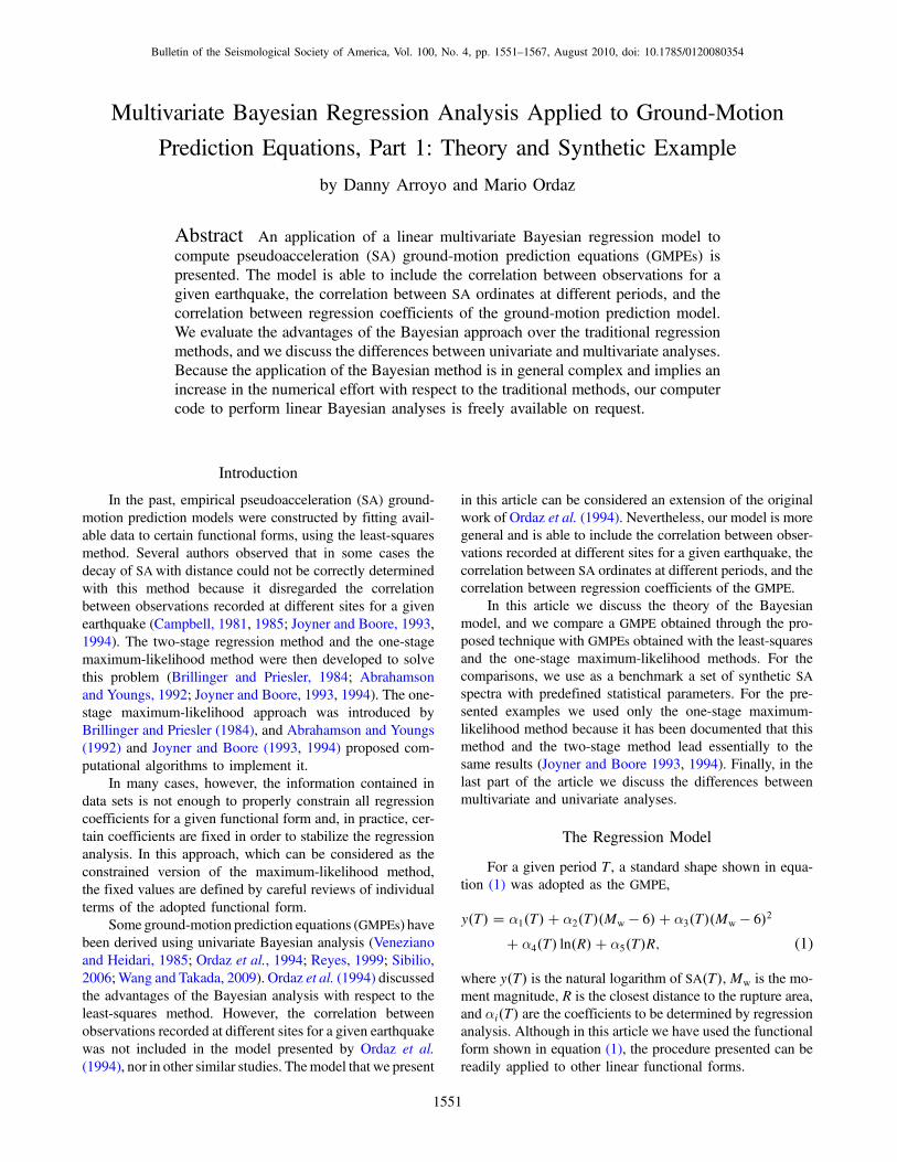
we have only 5 earthquakes recorded at 10 different stations.In addition, in Figure 3 we have plotted the standard devia-tion of the regression coefficients, that is, the square root ofthe diagonal elements of the covariance matrix defined inequation (10), as a function of T. As no increases, the scatterof regression parameters decreases.

Results for the One-Stage Maximum-Likelihood Method

Figure 4 shows a comparison of regression parametersobtained with the one-stage maximum-likelihood methodand the benchmark. The results are very similar to thoseobserved for the least-squares method. In general, the one-stage maximum-likelihood method is not able to attain thebenchmark values, except for α2�T� and σ. The greater dif-ferences between least-squares and one-stage maximum-likelihood methods are observed for α1�T� and α4�T�, for

Table 2αp and σ2 Used to Generate the Synthetic SA Spectra

T (sec) α1 α2 α3 α4 α5 σ2

0.0 5.8929 1.2457 �0:09757 �0:5 �0:00632 0.176260.1 6.0831 1.1954 �0:09668 �0:5 �0:00643 0.187840.2 6.7942 1.0675 �0:09858 �0:5 �0:00732 0.184940.3 6.9623 1.1303 �0:10357 �0:5 �0:00768 0.151070.4 6.7632 1.2513 �0:09682 �0:5 �0:00727 0.195490.5 6.9039 1.2236 �0:08753 �0:5 �0:00753 0.173970.6 6.5941 1.2748 �0:06768 �0:5 �0:00693 0.189360.7 6.7755 1.3445 �0:04662 �0:5 �0:0076 0.204630.8 6.5941 1.3676 �0:03662 �0:5 �0:00705 0.200440.9 6.4534 1.347 �0:0244 �0:5 �0:00648 0.183761.0 6.5638 1.3387 �0:05429 �0:5 �0:00665 0.182971.2 6.6903 1.3167 �0:05225 �0:5 �0:00723 0.198701.4 6.4825 1.3203 �0:06347 �0:5 �0:00662 0.210551.6 6.4614 1.4268 �0:10542 �0:5 �0:00632 0.234121.8 6.0912 1.4088 �0:09393 �0:5 �0:00516 0.277862.0 5.8698 1.3854 �0:05267 �0:5 �0:00505 0.288472.2 5.8367 1.4032 �0:04392 �0:5 �0:00547 0.352292.4 5.838 1.4032 �0:07922 �0:5 �0:00559 0.339162.6 5.858 1.3951 �0:06917 �0:5 �0:00601 0.345232.8 5.6616 1.3937 �0:0717 �0:5 �0:00583 0.335643.0 5.4214 1.4344 �0:0608 �0:5 �0:00568 0.349683.5 4.6026 1.4899 �0:06365 �0:5 �0:00438 0.331144.0 3.6367 1.5601 �0:05951 �0:5 �0:00283 0.355944.5 3.098 1.4864 �0:05698 �0:5 �0:00187 0.400885.0 3.2887 1.5282 �0:03953 �0:5 �0:00364 0.44147


which slightly better estimates are obtained with the least-squares method. In Figure 5, the standard deviation of theregression coefficients is shown; the trends are similar tothose observed for the least-squares method. Slightly largervalues of standard deviation are observed for the maximum-likelihood method than those obtained with the least-squares

method. In Table 3 estimates of γe related to different sets areshown; very accurate estimates are observed with no ≥ 200.

Prior Information for the Bayesian Method

In this section we present a short discussion about howto define the prior information for the Bayesian analysis. Wehave not included a sound discussion because a syntheticexample is presented. In a companion article (Arroyo andOrdaz, 2010) we use a set of actual ground-motion recordsand we present a complete discussion on how the prior in-formation can be defined.

The elements of α0 were set as follows. With theamplitude Fourier spectra defined by Brune’s model (Brune,1970) and common attenuation factors, and using randomvibration theory, we constructed a set of SA spectra relatedto several values of Mw and R (McGuire and Hanks, 1980;Boore, 1983). Then, we fit the values so computed to thefunctional form using the least-squares method in order tocompute α0; the elements of α0 obtained are shown inTable 4. This implies that a prioriwe believe that the attenua-tion of SA spectra can be properly characterized by Brune’smodel and common attenuation factors.

The block-symmetric matrix Δ is the prior covariancematrix of αV and can be written as

Figure 1. PGA attenuation with distance for the synthetic dataused in this study (sixth synthetic set, Table 1).

Figure 2. Results for least-squares method (benchmark values are plotted with a thick line).


Δ �

δ11 δ12 � � � δ1npδ22 � � � δ2np

. .. ..

.

δnpnp

26664

37775; (29)

where δij is an nT × nT symmetric matrix defined in equa-tion (30):

δij �

cov�αiT1;αjT1

� cov�αiT1;αjT2

� � � � cov�αiT1;αjTnT

�cov�αiT2

;αjT2� � � � cov�αiT2

;αjTnT�

. .. ..

.

cov�αiTnT;αjTnT

�

26664

37775: (30)

In equation (30) cov�αiTk;αjTl

� is the prior covariancebetween the coefficient αi�T� for the period Tk and thecoefficient αj�T� for the period Tl. The matrix Δ was setas diagonal; therefore, only the diagonal elements of δ11,δ22, δ33, δ44, and δ55 are different from zero. This impliesthat a priori we believe that the different αi�T� random vari-ables are uncorrelated. We set that structure for Δ because,from the presented example, we do not have informationabout correlation between the different αi�T�. Because the

coefficient α1�T� in equation (1) depends on site effects(Ordaz et al., 1994), we assigned a large value, with respectto the prior mean value of α1�T�, to the diagonal elements ofδ11. This implies that α1�T� is not controlled by its priormean value, so it is free to attain the value that yields thebest fit in the regression analysis. In the computations weused cov�α1TK

;α1TK� � 10; 000. For δ22, δ33, and δ44 we

assigned a value that implies a coefficient of variation of0.59 to their diagonal elements, as it was done in a previousstudy (Ordaz et al., 1994). Similarly to δ11, for the diagonalelements of δ55, we also used a large value with respect to theprior mean value of α5�T�; in the computations we usedcov�α5TK

;α5TK� � 1.

We set the diagonal elements ofΣ0 equal to 0.49, whichmeans that a priori we believe that the expected standarddeviation of the residuals is equal to 0.7, independently of

Figure 3. Standard deviation of the regression coefficients for the least-squares method (the symbols are the same as in Fig. 2).


Figure 4. Results for one-stage maximum-likelihood method (benchmark values are plotted with a thick line).

Figure 5. Standard deviation of the regression coefficients for the one-stage maximum-likelihood method (the symbols are the sameas in Fig. 4).


T. In addition, the off-diagonal terms were defined throughthe coefficient of correlation shown in equation (31):

ρ0T1;T2� exp��qjT1 � T2j�: (31)

Note that we use a very simple function to define the priorcorrelation between spectral ordinates of SA. According toequation (31), together with q � 1:0, the coefficient of cor-relation varies from unity, when T1 and T2 are equal, tonearly 0.05 when the difference between T1 and T2 is about3 sec. It must be acknowledged that equation (31) is quitearbitrary, and it was created only for the synthetic examplepresented in this article. When working with actual groundmotions it could be more reasonable to use the correlationcoefficients defined by Baker and Cornell (2006) as priorvalues. In the presented example we decided not to use

the equations of Baker and Cornell (2006) as prior informa-tion because they were used to generate the syntheticdata.

The degree of certainty of Σ0 depends on ν. As it hasbeen discussed, the larger the value of ν, the larger the degreeof certainty on Σ0. The posterior mean value of Σ can beexpressed as a weighted average between the prior meanvalue and the conditional weighted least-squares estimator.The weighting factors are ν=�no � ν� for the prior meanvalue and no=�no � ν� for the conditional weighted least-squares estimate. In the computations we have used a valueequal to 55 (the minimum required for nT � 25 in order togive a finite value to the covariance of Σ0) because we be-lieve that Σ0 is very uncertain. For no � 100 the weightingfactor for prior information is about 0.35.

Finally, our prior information of γe is vague, so we haveset a � b � 1:5, which is a very flat density, with meanvalue equal to 0.5, in order to force γe to take the value thatyields the best fit to data.

Results for the Bayesian Model

In order to exemplify the convergence of the Gibbs sam-pling, Figure 6 shows a comparison between estimates ofregression parameters for K ranging between 50 and 200.As has been stated, any value of �Σ0 and �γe0 could be usedas the starting value; for the computations we set �γe0 � 0 and�Σ0 � I. In addition, the prior mean values used in the anal-ysis are plotted in Figure 6. We observed that the Gibbs sam-pling method converges for relatively small values of K.Although not shown, similar trends were observed for othervalues of no. In Table 5 convergence of the Gibbs samplingregarding γe is presented; γe also converges for K between100 and 200. We note that these trends are valid only for thepresented example; for other cases of analysis it is recom-mended to build plots similar to Figure 6 in order to assessthe convergence of the Gibbs sampling. The value of Kshould be chosen carefully because computation time re-quired for the analysis grows with K. In order to minimizethe computational effort, the peak value of K used in theBayesian analysis was 500.

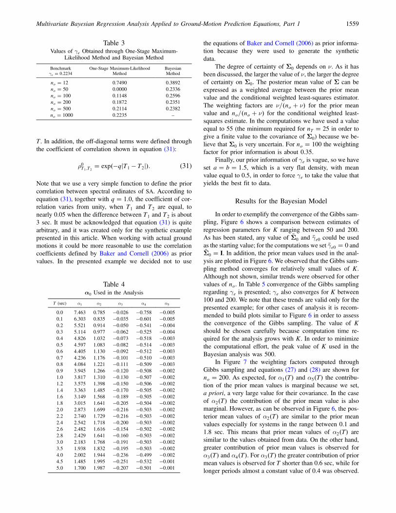
In Figure 7 the weighting factors computed throughGibbs sampling and equations (27) and (28) are shown forno � 200. As expected, for α1�T� and α5�T� the contribu-tion of the prior mean values is marginal because we set,a priori, a very large value for their covariance. In the caseof α2�T� the contribution of the prior mean value is alsomarginal. However, as can be observed in Figure 6, the pos-terior mean values of α2�T� are similar to the prior meanvalues especially for systems in the range between 0.1 and1.8 sec. This means that prior mean values of α2�T� aresimilar to the values obtained from data. On the other hand,greater contribution of prior mean values is observed forα3�T� and α4�T�. For α3�T� the greater contribution of priormean values is observed for T shorter than 0.6 sec, while forlonger periods almost a constant value of 0.4 was observed.

Table 3Values of γe Obtained through One-Stage Maximum-

Likelihood Method and Bayesian Method

Benchmarkγe � 0:2234

One-Stage Maximum-LikelihoodMethod

BayesianMethod

no � 12 0.7490 0.3892no � 50 0.0000 0.2336no � 100 0.1148 0.2596no � 200 0.1872 0.2351no � 500 0.2114 0.2382no � 1000 0.2235 –

Table 4α0 Used in the Analysis

T (sec) α1 α2 α3 α4 α5

0.0 7.463 0.785 �0:026 �0:758 �0:0050.1 6.303 0.835 �0:035 �0:601 �0:0050.2 5.521 0.914 �0:050 �0:541 �0:0040.3 5.114 0.977 �0:062 �0:525 �0:0040.4 4.826 1.032 �0:073 �0:518 �0:0030.5 4.597 1.083 �0:082 �0:514 �0:0030.6 4.405 1.130 �0:092 �0:512 �0:0030.7 4.236 1.176 �0:101 �0:510 �0:0030.8 4.084 1.221 �0:111 �0:509 �0:0030.9 3.945 1.266 �0:120 �0:508 �0:0021.0 3.817 1.310 �0:130 �0:507 �0:0021.2 3.575 1.398 �0:150 �0:506 �0:0021.4 3.363 1.485 �0:170 �0:505 �0:0021.6 3.149 1.568 �0:189 �0:505 �0:0021.8 3.015 1.641 �0:205 �0:504 �0:0022.0 2.873 1.699 �0:216 �0:503 �0:0022.2 2.740 1.729 �0:216 �0:503 �0:0022.4 2.542 1.718 �0:200 �0:503 �0:0022.6 2.482 1.616 �0:154 �0:502 �0:0022.8 2.429 1.641 �0:160 �0:503 �0:0023.0 2.183 1.768 �0:191 �0:503 �0:0023.5 1.938 1.832 �0:195 �0:503 �0:0024.0 2.002 1.944 �0:236 �0:499 �0:0024.5 1.485 1.995 �0:251 �0:532 �0:0015.0 1.700 1.987 �0:207 �0:501 �0:001


For α4�T� a nearly constant value of 0.9 is observed. We notethat in both cases the posterior mean values are close to theirprior counterparts, independent of Wp; this observation willbe discussed later in the article.

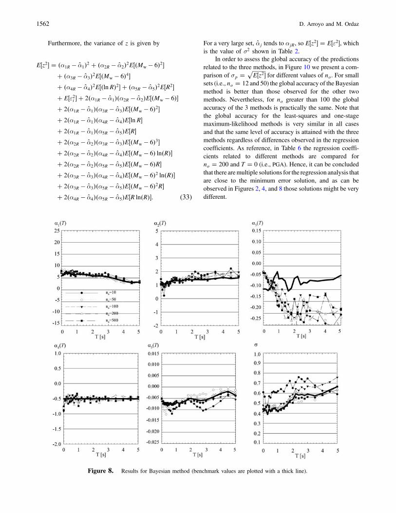
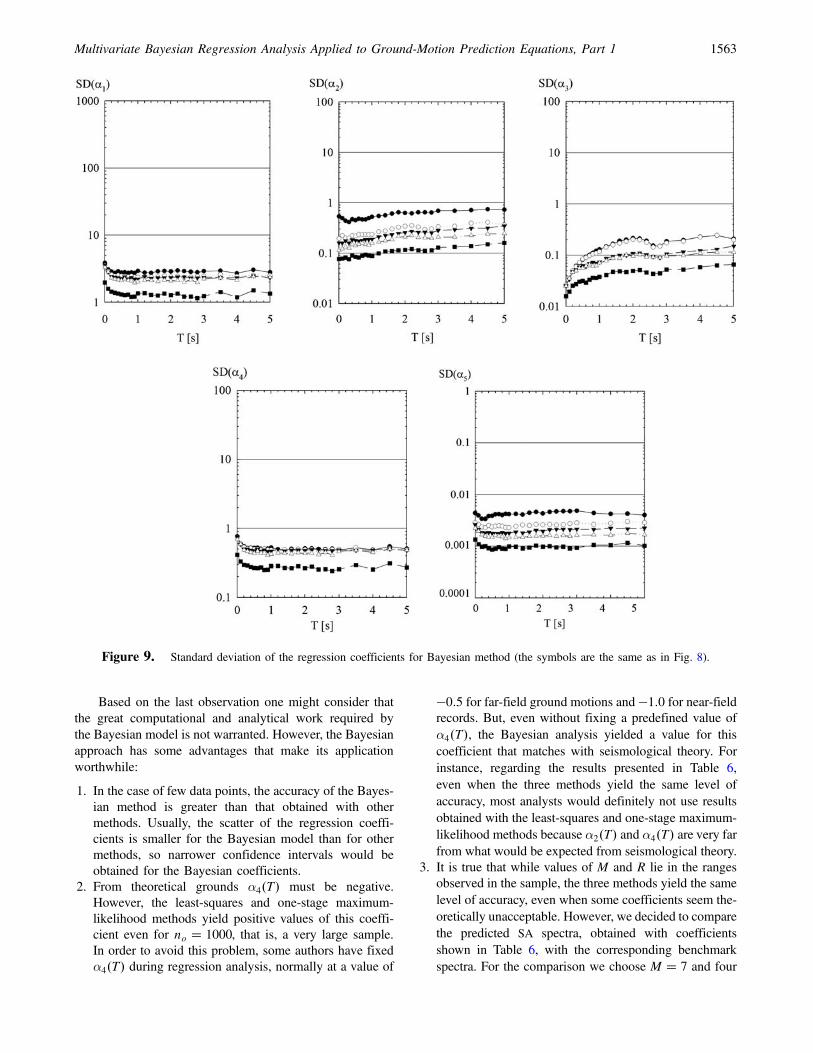
The results obtained with the Bayesian model are pre-sented in Figures 8 and 9. Conversely to what happened withother models, the Bayesian model was able to attain bench-mark values, except for α3�T�. Note that with no between100 and 200 very accurate estimates of the regression param-eters are observed. In general, the scatter of the Bayesianregression coefficients is smaller than that observed withother methods, which is an advantage of the Bayesian ap-proach over other methods. In Table 3 estimates of γe relatedto different sets are shown; accurate estimates are observedfor no greater than 50. Note that in spite of our use of a priormean value of γe � 0:5 the data shifted the prior mean valueto the correct value of γe.

As has been stated, the Bayesian method was not able toattain the correct value of α3�T�. According to Figure 8, asno increases, slightly better estimates are observed, espe-cially for T larger than 2 sec. However, in general, posteriormean values are close to prior mean values of α3�T�, even ifthe weighting factor decreases. For example, in Figure 7 itcan be seen that for no � 200, Wp is about 0.4 in the long-period range, while for no � 500 (although not shown) aWp

Figure 6. Convergence of Gibbs sampling for the set with no � 200 (prior values are plotted with a thick line).

Table 5Convergence of γe for no � 200

Prior γe � 0:5

K � 12 γe � 0:2367

K � 50 γe � 0:2338K � 100 γe � 0:2353K � 200 γe � 0:2351


value about 0.2 was observed. This means that informationcontained in the data is not enough to completely defineα3�T�; in other words, α3�T� has little effect on y and almostany value could have been used. Hence, the Bayesianmethod, instead of leading to any value of α3�T� (such asother methods) leads to values of α3�T� that are close to itsprior mean value.

Discussion

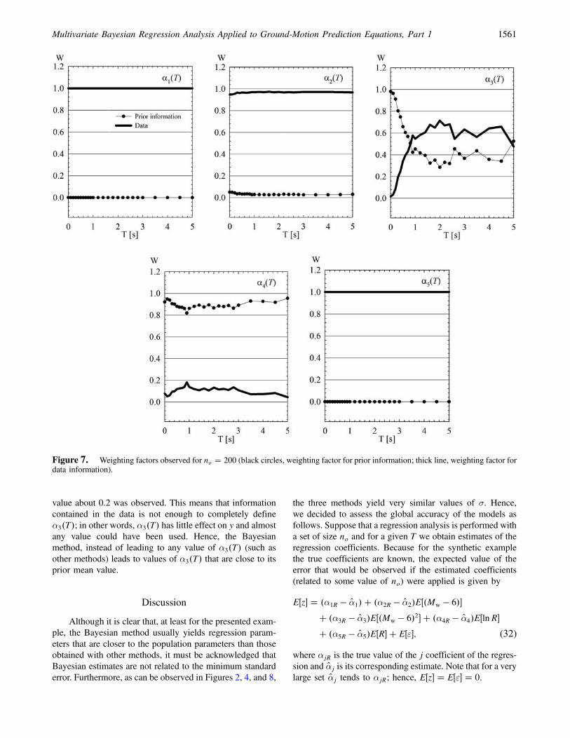
Although it is clear that, at least for the presented exam-ple, the Bayesian method usually yields regression param-eters that are closer to the population parameters than thoseobtained with other methods, it must be acknowledged thatBayesian estimates are not related to the minimum standarderror. Furthermore, as can be observed in Figures 2, 4, and 8,

the three methods yield very similar values of σ. Hence,we decided to assess the global accuracy of the models asfollows. Suppose that a regression analysis is performed witha set of size no and for a given T we obtain estimates of theregression coefficients. Because for the synthetic examplethe true coefficients are known, the expected value of theerror that would be observed if the estimated coefficients(related to some value of no) were applied is given by

E�z� � �α1R � α̂1� � �α2R � α̂2�E��Mw � 6�� α3R � α̂3�E��Mw � 6�2� � �α4R � α̂4�E�lnR�� α5R � α̂5�E�R� � E�ε�; (32)

where αjR is the true value of the j coefficient of the regres-sion and α̂j is its corresponding estimate. Note that for a verylarge set α̂j tends to αjR; hence, E�z� � E�ε� � 0.

Figure 7. Weighting factors observed for no � 200 (black circles, weighting factor for prior information; thick line, weighting factor fordata information).


Furthermore, the variance of z is given by

E�z2� � �α1R � α̂1�2 � �α2R � α̂2�2E��Mw � 6�2�� α3R � α̂3�2E��Mw � 6�4�� α4R � α̂4�2E��lnR�2� � �α5R � α̂5�2E�R2�� E�ε2i � � 2�α1R � α̂1��α2R � α̂2�E��Mw � 6�� 2�α1R � α̂1��α3R � α̂3�E��Mw � 6�2�� 2�α1R � α̂1��α4R � α̂4�E�lnR�� 2�α1R � α̂1��α5R � α̂5�E�R�� 2�α2R � α̂2��α3R � α̂3�E��Mw � 6�3�� 2�α2R � α̂2��α4R � α̂4�E��Mw � 6� ln�R�� 2�α2R � α̂2��α5R � α̂5�E��Mw � 6�R�� 2�α3R � α̂3��α4R � α̂4�E��Mw � 6�2 ln�R�� 2�α3R � α̂3��α5R � α̂5�E��Mw � 6�2R�� 2�α4R � α̂4��α5R � α̂5�E�R ln�R��: (33)

For a very large set, α̂j tends to αjR, so E�z2� � E�ε2�, whichis the value of σ2 shown in Table 2.

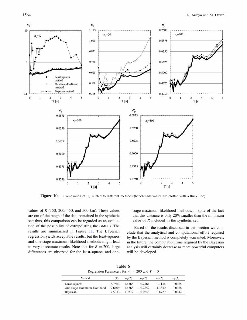
In order to assess the global accuracy of the predictionsrelated to the three methods, in Figure 10 we present a com-parison of σp �

��E�z2�

pfor different values of no. For small

sets (i.e., no � 12 and 50) the global accuracy of the Bayesianmethod is better than those observed for the other twomethods. Nevertheless, for no greater than 100 the globalaccuracy of the 3 methods is practically the same. Note thatthe global accuracy for the least-squares and one-stagemaximum-likelihood methods is very similar in all casesand that the same level of accuracy is attained with the threemethods regardless of differences observed in the regressioncoefficients. As reference, in Table 6 the regression coeffi-cients related to different methods are compared forno � 200 and T � 0 (i.e., PGA). Hence, it can be concludedthat there aremultiple solutions for the regression analysis thatare close to the minimum error solution, and as can beobserved in Figures 2, 4, and 8 those solutions might be verydifferent.

Figure 8. Results for Bayesian method (benchmark values are plotted with a thick line).


Based on the last observation one might consider thatthe great computational and analytical work required bythe Bayesian model is not warranted. However, the Bayesianapproach has some advantages that make its applicationworthwhile:

1. In the case of few data points, the accuracy of the Bayes-ian method is greater than that obtained with othermethods. Usually, the scatter of the regression coeffi-cients is smaller for the Bayesian model than for othermethods, so narrower confidence intervals would beobtained for the Bayesian coefficients.

2. From theoretical grounds α4�T� must be negative.However, the least-squares and one-stage maximum-likelihood methods yield positive values of this coeffi-cient even for no � 1000, that is, a very large sample.In order to avoid this problem, some authors have fixedα4�T� during regression analysis, normally at a value of

�0:5 for far-field ground motions and �1:0 for near-fieldrecords. But, even without fixing a predefined value ofα4�T�, the Bayesian analysis yielded a value for thiscoefficient that matches with seismological theory. Forinstance, regarding the results presented in Table 6,even when the three methods yield the same level ofaccuracy, most analysts would definitely not use resultsobtained with the least-squares and one-stage maximum-likelihood methods because α2�T� and α4�T� are very farfrom what would be expected from seismological theory.

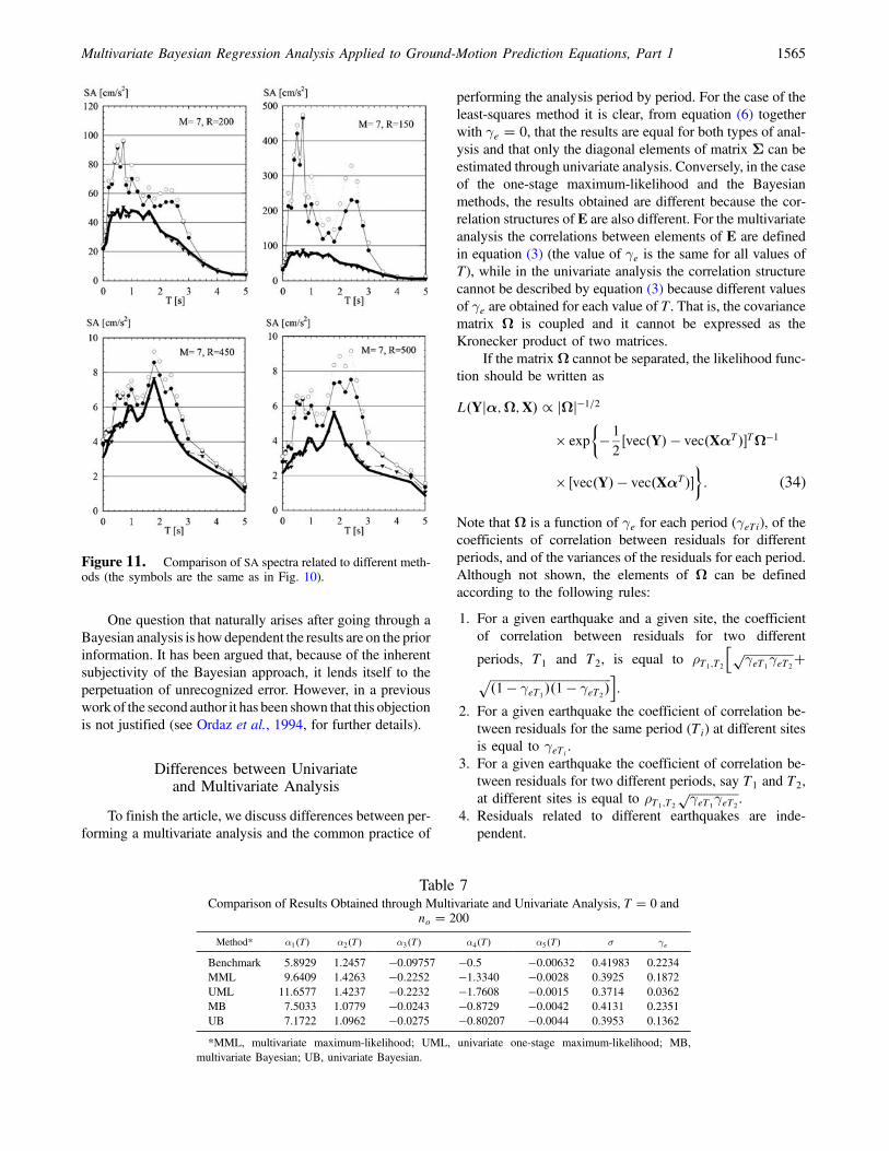
3. It is true that while values of M and R lie in the rangesobserved in the sample, the three methods yield the samelevel of accuracy, even when some coefficients seem the-oretically unacceptable. However, we decided to comparethe predicted SA spectra, obtained with coefficientsshown in Table 6, with the corresponding benchmarkspectra. For the comparison we choose M � 7 and four

Figure 9. Standard deviation of the regression coefficients for Bayesian method (the symbols are the same as in Fig. 8).


values of R (150, 200, 450, and 500 km). These valuesare out of the range of the data contained in the syntheticset; thus, this comparison can be regarded as an evalua-tion of the possibility of extrapolating the GMPEs. Theresults are summarized in Figure 11. The Bayesianregression yields acceptable results, but the least-squaresand one-stage maximum-likelihood methods might leadto very inaccurate results. Note that for R � 200, largedifferences are observed for the least-squares and one-

stage maximum-likelihood methods, in spite of the factthat this distance is only 20% smaller than the minimumvalue of R included in the synthetic set.

Based on the results discussed in this section we con-clude that the analytical and computational effort requiredby the Bayesian method is completely warranted. Moreover,in the future, the computation time required by the Bayesiananalysis will certainly decrease as more powerful computerswill be developed.

Figure 10. Comparison of σp related to different methods (benchmark values are plotted with a thick line).

Table 6Regression Parameters for no � 200 and T � 0

Method α1�T� α2�T� α3�T� α4�T� α5�T�Least-squares 3.7863 1.4263 �0:2264 �0:1136 �0:0065One-stage maximum-likelihood 9.6409 1.4263 �0:2252 �1:3340 �0:0028Bayesian 7.5033 1.0779 �0:0243 �0:8729 �0:0042


One question that naturally arises after going through aBayesian analysis is howdependent the results are on the priorinformation. It has been argued that, because of the inherentsubjectivity of the Bayesian approach, it lends itself to theperpetuation of unrecognized error. However, in a previouswork of the second author it has been shown that this objectionis not justified (see Ordaz et al., 1994, for further details).

Differences between Univariateand Multivariate Analysis

To finish the article, we discuss differences between per-forming a multivariate analysis and the common practice of

performing the analysis period by period. For the case of theleast-squares method it is clear, from equation (6) togetherwith γe � 0, that the results are equal for both types of anal-ysis and that only the diagonal elements of matrix Σ can beestimated through univariate analysis. Conversely, in the caseof the one-stage maximum-likelihood and the Bayesianmethods, the results obtained are different because the cor-relation structures of E are also different. For the multivariateanalysis the correlations between elements of E are definedin equation (3) (the value of γe is the same for all values ofT), while in the univariate analysis the correlation structurecannot be described by equation (3) because different valuesof γe are obtained for each value of T. That is, the covariancematrix Ω is coupled and it cannot be expressed as theKronecker product of two matrices.

If the matrixΩ cannot be separated, the likelihood func-tion should be written as

L�Yjα;Ω;X� ∝ jΩj�1=2

× exp�� 1

2�vec�Y� � vec�XαT��TΩ�1

× �vec�Y� � vec�XαT��: (34)

Note that Ω is a function of γe for each period (γeTi), of thecoefficients of correlation between residuals for differentperiods, and of the variances of the residuals for each period.Although not shown, the elements of Ω can be definedaccording to the following rules:

1. For a given earthquake and a given site, the coefficientof correlation between residuals for two different

periods, T1 and T2, is equal to ρT1;T2

h ��γeT1γeT2

p ��1 � γeT1

��1 � γeT2�p i.

2. For a given earthquake the coefficient of correlation be-tween residuals for the same period (Ti) at different sitesis equal to γeTi

.3. For a given earthquake the coefficient of correlation be-

tween residuals for two different periods, say T1 and T2,at different sites is equal to ρT1;T2

��γeT1γeT2

p .4. Residuals related to different earthquakes are inde-

pendent.

Figure 11. Comparison of SA spectra related to different meth-ods (the symbols are the same as in Fig. 10).

Table 7Comparison of Results Obtained through Multivariate and Univariate Analysis, T � 0 and

no � 200

Method* α1�T� α2�T� α3�T� α4�T� α5�T� σ γe

Benchmark 5.8929 1.2457 �0:09757 �0:5 �0:00632 0.41983 0.2234MML 9.6409 1.4263 �0:2252 �1:3340 �0:0028 0.3925 0.1872UML 11.6577 1.4237 �0:2232 �1:7608 �0:0015 0.3714 0.0362MB 7.5033 1.0779 �0:0243 �0:8729 �0:0042 0.4131 0.2351UB 7.1722 1.0962 �0:0275 �0:80207 �0:0044 0.3953 0.1362

*MML, multivariate maximum-likelihood; UML, univariate one-stage maximum-likelihood; MB,multivariate Bayesian; UB, univariate Bayesian.


The one-stage maximum-likelihood method for thiscorrelation structure consists of maximizing equation (34).However, the maximization process is much more complexthan in the case of a single γe for all periods becausemaximization must be carried out considering simulta-neously all the coefficients of correlation between residuals,all the γeTi

parameters, and all the variances of the residuals.Also, the Bayesian model becomes very complex if differentvalues of γe are adopted for each period because priordensities for all γeTi

and those parameters are coupled withthe variances of the residuals and with the coefficients ofcorrelation between residuals for different periods. Becausewe consider that the application of this Bayesian modelwould be impractical, the complete analysis is not presentedin this article. However, the complete analysis can be ob-tained following the procedure presented in the section titledThe Bayesian Model.

Thus, the common practice of performing the analysisperiod by period implicitly disregards the correlation be-tween residuals for different periods. The influence of thisassumption in the accuracy of the GMPE depends on howlarge this correlation is. In Table 7 we present a comparisonof regression parameters obtained through multivariatemaximum-likelihood, multivariate Bayesian, univariate one-stage maximum-likelihood, and univariate Bayesian meth-ods for no � 200 and T � 0 (i.e., PGA). Unsurprisingly,the multivariate results are closer to the benchmark values,especially for γe, because the synthetic data were generatedwith the correlation structure defined in equation (3).Nevertheless, in the case of data obtained from actual groundmotions, the true correlation structure is unknown; hence,we cannot consider that the multivariate analysis is moreaccurate than the univariate analysis based only in the resultspresented in Table 7. However, from the discussion presentedin this section we consider that the multivariate regressionmodel is theoretically more robust than the common practiceof performing the analysis period by period.

It is interesting to note that during the computations weobserved that the time required in the Bayesian analysis forthe univariate and the multivariate cases is almost the samebecause the rank of matrix Φ is equal in both cases. Inpractice, an approach that can be used is to perform theunivariate analysis and include the correlation between spec-tral ordinates through the copula technique described inGoda and Atkinson (2009).

Conclusions

We have presented a linear multivariate Bayesian regres-sion method that includes the correlation between observa-tions for a given earthquake, the correlation between SAordinates at different periods, and the correlation betweenregression coefficients of the GMPE. Through comparisonsof GMPEs obtained with the least-squares and the one-stagemaximum-likelihood methods we have shown that multiplesolutions close to minimum error could exist and that the

Bayesian method could be used to obtain a GMPE consistentwith seismological theory. In addition, for the presented syn-thetic example, it is shown that GMPEs obtained throughBayesian analysis yield more accurate results than GMPEsrelated to other methods when the GMPEs are extrapolated.However, the Bayesian method requires significantly moreanalytical and computational work than traditional methods.Hence, our computer code to perform linear Bayesian ana-lyses is freely available on request.

Data and Resources

No actual data were used in this article. The syntheticdata are available on request.

Acknowledgments

The authors appreciate the efforts of two anonymous reviewers,who greatly contributed to improve the original manuscript. Constructivecomments by Gail Atkinson are also appreciated.

References

Abrahamson, N. A., and R. R. Youngs (1992). A stable algorithm for regres-sion analysis using the random effects model, Bull. Seismol. Soc. Am.82, 505–510.

Arroyo, D., and M. Ordaz (2010). Multivariate Bayesian regression analysisapplied to ground motion prediction equations, Part 2: Numerical ex-ample with actual data, Bull. Seismol. Soc. Am. 100, 1568–1577.

Baker, J. W., and C. A. Cornell (2006). Correlation of response spectralvalues for multicomponent ground motions, Bull. Seismol. Soc. Am.96, 215–227.

Boore, D. M. (1983). Stochastic simulation of high-frequency groundmotions based on seismological models of the radiated spectra, Bull.Seismol. Soc. Am. 73, no. 6, 1865–1894.

Boore, D. M., J. F. Gibbs, W. B. Joyner, J. C. Tinsley, and D. J. Ponti (2003).Estimated ground motion from the 1994 Northridge, California, earth-quake at the site of the Interstate 10 and La Cienega boulevard bridgecollapse, west Los Angeles, California, Bull. Seismol. Soc. Am. 93,2737–2751.

Brillinger, D. R., and H. K. Preisler (1984). An exploratory analysis of theJoyner–Boore attenuation data, Bull. Seismol. Soc. Am. 74, 1441–1450.

Broemeling, L. D. (1985). Bayesian Analysis of Linear Models, Marcel Dek-ker, New York, 454 pp.

Brune, J. N. (1970). Tectonic stresses and spectra of seismic waves fromearthquakes, J. Geophys. Res. 75, 4997–5009.

Campbell, K. W. (1981). Near-source attenuation of peak horizontal accel-eration, Bull. Seismol. Soc. Am. 71, 2039–2070.

Campbell, K. W. (1985). Strong motion attenuation relations: A ten-yearperspective, Earthq. Spectra 1, no. 4, 759–804.

Geman, S., and D. Geman (1984). Stochastic relaxation, Gibbs distributions,and the Bayesian restoration of images, IEEE Trans. Pattern Anal.Mach. Intell. 6, 721–741.

Goda, K., and G. M. Atkinson (2009). Interperiod dependence ofground-motion prediction equations: A copula perspective, Bull.Seismol. Soc. Am. 99, no. 2A, 922–927.

Joyner, W. B., and D. M. Boore (1993). Methods for regression analysisof strong-motion data, Bull. Seismol. Soc. Am. 83, no. 2,469–487.

Joyner, W. B., and D. M. Boore (1994). Errata: Methods for regressionanalysis of strong-motion data, Bull. Seismol. Soc. Am. 84, no. 3,955–956.


Kawakami, H, and H. Mogi (2003). Analyzing spatial intraevent variabilityof peak ground accelerations as a function of separation distance, Bull.Seismol. Soc. Am. 93, 1079–1090.

McGuire, R. K., and T. C. Hanks (1980). RMS accelerations andspectral amplitudes of strong ground motion during the SanFernando, California, earthquake, Bull. Seismol. Soc. Am. 70, no. 5,1907–1919.

Ordaz, M., S. K. Singh, and A. Arciniega (1994). Bayesian attenuationregressions: An application to Mexico City, Geophys. J. Int. 117,335–344.

Reyes, C. (1999). El estado límite de servicio en el diseño sísmico deedificios, Ph.D. Thesis, School of Engineering, UNAM.

Rowe, D. B. (2002). Multivariate Bayesian Statistics: Models for SourceSeparation and Signal Unmixing, Chapman & Hall/CRC, New York,329 pp.

Sibilio, E. (2006). Seismic risk assessment of structures by means of stochas-tic simulation techniques, Ph.D. Thesis, Braunschweig TechnicalUniversity and Florence University.

Veneziano, D., and M. Heidari (1985). Statistical analysis of attenuation inthe eastern United States, in Methods of Earthquake Ground-MotionEstimation for the Eastern United States, EPRI Research ProjectRP2556-16, Palo Alto, California.

Wang, M., and T. Takada (2005). Macrospatial correlation model of seismicground motions, Earthq. Spectra 21, 1137–1156.

Wang, M., and T. Takada (2009). A Bayesian framework for prediction ofseismic ground motion, Bull. Seismol. Soc. Am. 99, no. 4, 2348–2364.

Departamento de MaterialesUniversidad Autónoma Metropolitana-AzcapotzalcoAv. San Pablo # 180. Colonia Reynosa TamaulipasAzcapotzalco CP 02200México D.F., Mé[email protected]

(D.A.)

Instituto de IngenieríaUNAM Ciudad UniversitariaCoyoacán CP 04510México D.F. Mé[email protected]

(M.O.)

Manuscript received 3 December 2008


multivariate bayesian regression analysis applied...

Documents