multiscale mixed finite-element methods for simulation … · multiscale mixed finite-element...
TRANSCRIPT
Multiscale Mixed Finite-Element Methods forSimulation of Flow in Highly Heterogeneous
Porous Media
Knut–Andreas Lie
SINTEF ICT, Dept. Applied Mathematics
Fifth China-Norway-Sweden Workshop on ComputationalMathematics, Lund, June 5–7, 2006
Applied Mathematics June 2006 1/30
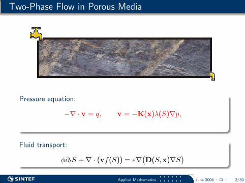
Two-Phase Flow in Porous Media
Pressure equation:
−∇ · v = q, v = −K(x)λ(S)∇p,
Fluid transport:
φ∂tS +∇ · (vf(S)) = ε∇(D(S,x)∇S
)Applied Mathematics June 2006 2/30
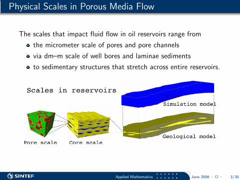
Physical Scales in Porous Media Flow
The scales that impact fluid flow in oil reservoirs range from
the micrometer scale of pores and pore channels
via dm–m scale of well bores and laminae sediments
to sedimentary structures that stretch across entire reservoirs.
Applied Mathematics June 2006 3/30
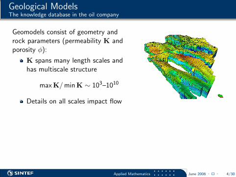
Geological ModelsThe knowledge database in the oil company
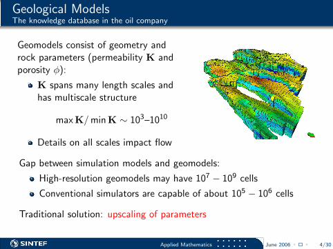
Geomodels consist of geometry androck parameters (permeability K andporosity φ):
K spans many length scales andhas multiscale structure
maxK/minK ∼ 103–1010
Details on all scales impact flow
Gap between simulation models and geomodels:
High-resolution geomodels may have 107 − 109 cells
Conventional simulators are capable of about 105 − 106 cells
Traditional solution: upscaling of parameters
Applied Mathematics June 2006 4/30
Geological ModelsThe knowledge database in the oil company
Geomodels consist of geometry androck parameters (permeability K andporosity φ):
K spans many length scales andhas multiscale structure
maxK/minK ∼ 103–1010
Details on all scales impact flow
Gap between simulation models and geomodels:
High-resolution geomodels may have 107 − 109 cells
Conventional simulators are capable of about 105 − 106 cells
Traditional solution: upscaling of parameters
Applied Mathematics June 2006 4/30
Upscaling the Pressure Equation
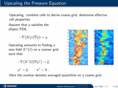
Upscaling: combine cells to derive coarse grid, determine effectivecell properties
Assume that p satisfies theelliptic PDE:
−∇(K(x)∇p
)= q.
Upscaling amounts to finding anew field K∗(x) on a coarser gridsuch that
−∇(K∗(x)∇p∗
)= q,
p∗ ∼ p, v∗ ∼ v .10 20 30 40 50 60
20
40
60
80
100
120
140
160
180
200
220
2 4 6 8 10
2
4
6
8
10
12
14
16
18
20
22
Here the overbar denotes averaged quantities on a coarse grid.
Applied Mathematics June 2006 5/30
Upscaling the Pressure Equation, cont’d
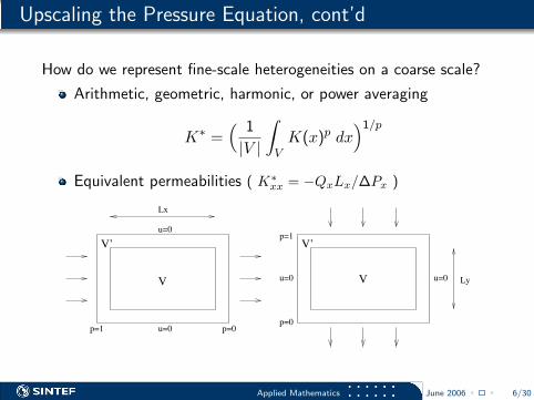
How do we represent fine-scale heterogeneities on a coarse scale?
Arithmetic, geometric, harmonic, or power averaging
K∗ =( 1
|V |
∫VK(x)p dx
)1/p
Equivalent permeabilities ( K∗xx = −QxLx/∆Px )
V’
p=1 p=0
u=0
u=0
V
p=1
p=0
u=0 u=0V
V’
Lx
Ly
Applied Mathematics June 2006 6/30
Vision — Fast Simulation of Geomodels
Vision:
Direct simulation of fluid flow on high-resolution geomodels ofhighly heterogeneous and fractured porous media in 3D.
Why multiscale methods?
Small-scale variations in the permeability can have a strong impacton large-scale flow and should be resolved properly. Observation:
the pressure may be well resolved on a coarse grid
the fluid transport should be solved on the finest scale possible
Thus: a multiscale method for the pressure equation should providevelocity fields that can be used to simulate flow on a fine scale
Applied Mathematics June 2006 7/30
Developing an Alternative to Upscaling
We seek a multiscale methodology that:
incorporates small-scale effects into the discretisation on acoarse scale
gives a detailed image of the flow pattern on the fine scale,without having to solve the full fine-scale system
is robust and flexible with respect to the coarse grid
is robust and flexible with respect to the fine grid and thefine-grid solver
is accurate and conservative
is fast and easy to parallelise
Applied Mathematics June 2006 8/30
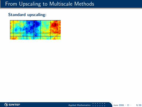
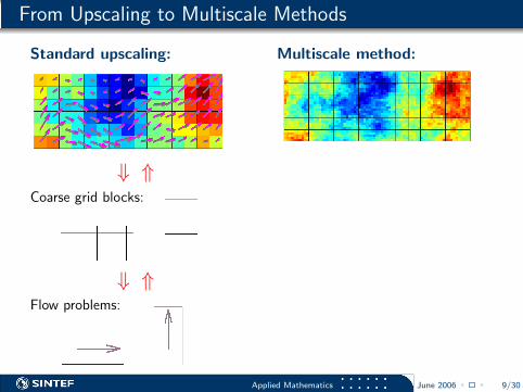
From Upscaling to Multiscale Methods
Standard upscaling:
⇓
⇑
Coarse grid blocks:⇓
⇑
Flow problems:
Multiscale method:
⇓
⇑
Coarse grid blocks:
⇓
⇑
Flow problems:
Applied Mathematics June 2006 9/30

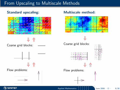
From Upscaling to Multiscale Methods
Standard upscaling:
⇓
⇑
Coarse grid blocks:
⇓
⇑
Flow problems:
Multiscale method:
⇓
⇑
Coarse grid blocks:
⇓
⇑
Flow problems:
Applied Mathematics June 2006 9/30

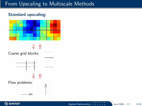
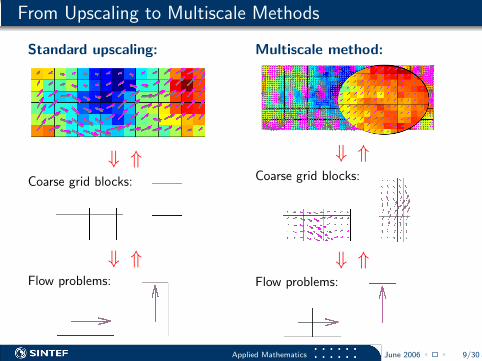
From Upscaling to Multiscale Methods
Standard upscaling:
⇓
⇑
Coarse grid blocks:
⇓
⇑
Flow problems:
Multiscale method:
⇓
⇑
Coarse grid blocks:
⇓
⇑
Flow problems:
Applied Mathematics June 2006 9/30
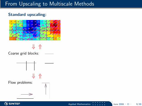
From Upscaling to Multiscale Methods
Standard upscaling:
⇓ ⇑Coarse grid blocks:
⇓ ⇑Flow problems:
Multiscale method:
⇓
⇑
Coarse grid blocks:
⇓
⇑
Flow problems:
Applied Mathematics June 2006 9/30
From Upscaling to Multiscale Methods
Standard upscaling:
⇓ ⇑Coarse grid blocks:
⇓ ⇑Flow problems:
Multiscale method:
⇓
⇑
Coarse grid blocks:
⇓
⇑
Flow problems:
Applied Mathematics June 2006 9/30
From Upscaling to Multiscale Methods
Standard upscaling:
⇓ ⇑Coarse grid blocks:
⇓ ⇑Flow problems:
Multiscale method:
⇓
⇑
Coarse grid blocks:
⇓
⇑
Flow problems:
Applied Mathematics June 2006 9/30

From Upscaling to Multiscale Methods
Standard upscaling:
⇓ ⇑Coarse grid blocks:
⇓ ⇑Flow problems:
Multiscale method:
⇓
⇑
Coarse grid blocks:
⇓
⇑
Flow problems:
Applied Mathematics June 2006 9/30
From Upscaling to Multiscale Methods
Standard upscaling:
⇓ ⇑Coarse grid blocks:
⇓ ⇑Flow problems:
Multiscale method:
⇓
⇑
Coarse grid blocks:
⇓ ⇑Flow problems:
Applied Mathematics June 2006 9/30
From Upscaling to Multiscale Methods
Standard upscaling:
⇓ ⇑Coarse grid blocks:
⇓ ⇑Flow problems:
Multiscale method:
⇓ ⇑Coarse grid blocks:
⇓ ⇑Flow problems:
Applied Mathematics June 2006 9/30
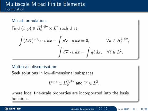
Multiscale Mixed Finite ElementsFormulation
Mixed formulation:
Find (v, p) ∈ H1,div0 × L2 such that∫
(λK)−1u · v dx−∫p∇ · u dx = 0, ∀u ∈ H1,div
0 ,∫`∇ · v dx =
∫q` dx, ∀` ∈ L2.
Multiscale discretisation:
Seek solutions in low-dimensional subspaces
Ums ⊂ H1,div0 and V ∈ L2,
where local fine-scale properties are incorporated into the basisfunctions.
Applied Mathematics June 2006 10/30
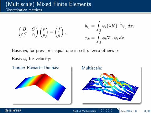
(Multiscale) Mixed Finite ElementsDiscretisation matrices
(B CCT 0
)(vp
)=
(fg
),
bij =
∫Ωψi
(λK)−1
ψj dx,
cik =
∫Ωφk∇ · ψi dx
Basis φk for pressure: equal one in cell k, zero otherwise
Basis ψi for velocity:
1.order Raviart–Thomas: Multiscale:
Applied Mathematics June 2006 11/30
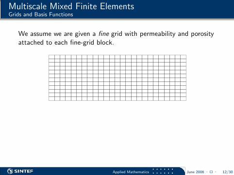
Multiscale Mixed Finite ElementsGrids and Basis Functions
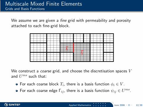
We assume we are given a fine grid with permeability and porosityattached to each fine-grid block.
We construct a coarse grid, and choose the discretisation spaces Vand Ums such that:
For each coarse block Ti, there is a basis function φi ∈ V .
For each coarse edge Γij , there is a basis function ψij ∈ Ums.
Applied Mathematics June 2006 12/30
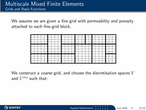
Multiscale Mixed Finite ElementsGrids and Basis Functions
We assume we are given a fine grid with permeability and porosityattached to each fine-grid block.
We construct a coarse grid, and choose the discretisation spaces Vand Ums such that:
For each coarse block Ti, there is a basis function φi ∈ V .
For each coarse edge Γij , there is a basis function ψij ∈ Ums.
Applied Mathematics June 2006 12/30
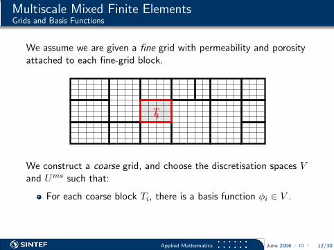
Multiscale Mixed Finite ElementsGrids and Basis Functions
We assume we are given a fine grid with permeability and porosityattached to each fine-grid block.
Ti
We construct a coarse grid, and choose the discretisation spaces Vand Ums such that:
For each coarse block Ti, there is a basis function φi ∈ V .
For each coarse edge Γij , there is a basis function ψij ∈ Ums.
Applied Mathematics June 2006 12/30
Multiscale Mixed Finite ElementsGrids and Basis Functions
We assume we are given a fine grid with permeability and porosityattached to each fine-grid block.
TiTj
We construct a coarse grid, and choose the discretisation spaces Vand Ums such that:
For each coarse block Ti, there is a basis function φi ∈ V .
For each coarse edge Γij , there is a basis function ψij ∈ Ums.
Applied Mathematics June 2006 12/30
Multiscale Mixed Finite ElementsBasis for the Velocity Field
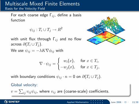
For each coarse edge Γij , define a basisfunction
ψij : Ti ∪ Tj → R2
with unit flux through Γij and no flowacross ∂(Ti ∪ Tj).
Homogeneous medium Heterogeneous medium
We use ψij = −λK∇φij with
∇ · ψij =
wi(x), for x ∈ Ti,
−wj(x), for x ∈ Tj ,
with boundary conditions ψij · n = 0 on ∂(Ti ∪ Tj).
Global velocity:
v =∑
ij vijψij , where vij are (coarse-scale) coefficients.
Applied Mathematics June 2006 13/30
Multiscale Mixed Finite ElementsBasis for Velocity - the Source Weights.
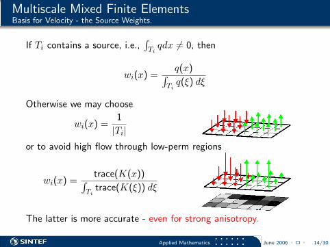
If Ti contains a source, i.e.,∫Tiqdx 6= 0, then
wi(x) =q(x)∫
Tiq(ξ) dξ
Otherwise we may choose
wi(x) =1
|Ti|or to avoid high flow through low-perm regions
wi(x) =trace(K(x))∫
Titrace(K(ξ)) dξ
The latter is more accurate - even for strong anisotropy.
Applied Mathematics June 2006 14/30
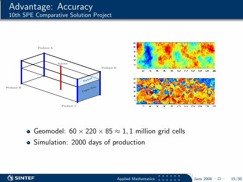
Advantage: Accuracy10th SPE Comparative Solution Project
Producer A
Producer B
Producer C
Producer D
Injector
Tarbert
UpperNess
Geomodel: 60× 220× 85 ≈ 1, 1 million grid cells
Simulation: 2000 days of production
Applied Mathematics June 2006 15/30
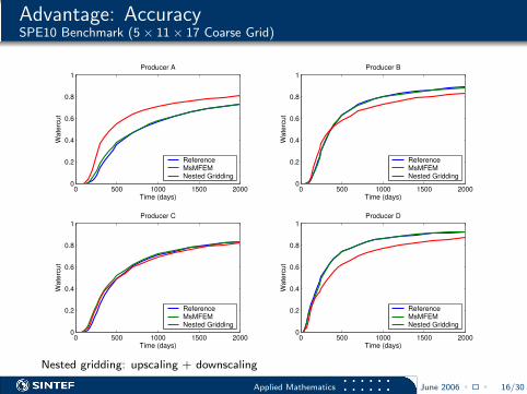
Advantage: AccuracySPE10 Benchmark (5× 11× 17 Coarse Grid)
0 500 1000 1500 20000
0.2
0.4
0.6
0.8
1
Time (days)
Wat
ercu
tProducer A
0 500 1000 1500 20000
0.2
0.4
0.6
0.8
1
Time (days)
Wat
ercu
t
Producer B
0 500 1000 1500 20000
0.2
0.4
0.6
0.8
1
Time (days)
Wat
ercu
t
Producer C
0 500 1000 1500 20000
0.2
0.4
0.6
0.8
1
Time (days)
Wat
ercu
t
Producer D
ReferenceMsMFEM Nested Gridding
ReferenceMsMFEM Nested Gridding
ReferenceMsMFEM Nested Gridding
ReferenceMsMFEM Nested Gridding
Nested gridding: upscaling + downscaling
Applied Mathematics June 2006 16/30
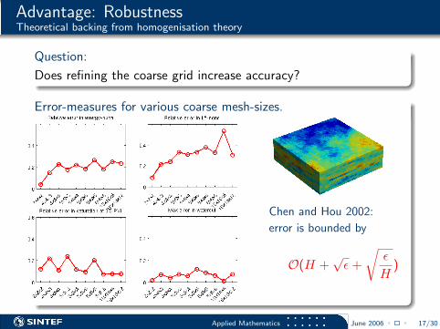
Advantage: RobustnessTheoretical backing from homogenisation theory
Question:
Does refining the coarse grid increase accuracy?
Error-measures for various coarse mesh-sizes.
Chen and Hou 2002:
error is bounded by
O(H +√ε+
√ε
H)
Applied Mathematics June 2006 17/30
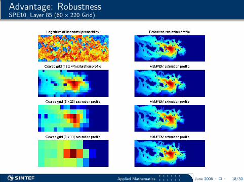
Advantage: RobustnessSPE10, Layer 85 (60× 220 Grid)
Applied Mathematics June 2006 18/30
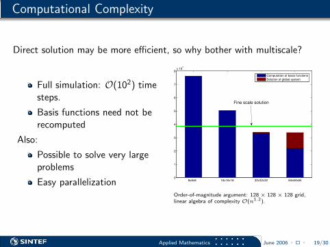
Computational Complexity
Direct solution may be more efficient, so why bother with multiscale?
Full simulation: O(102) timesteps.
Basis functions need not berecomputed
Also:
Possible to solve very largeproblems
Easy parallelization 8x8x8 16x16x16 32x32x32 64x64x640
1
2
3
4
5
6
7
8x 10⁷
Computation of basis functionsSolution of global system
Fine scale solution
Order-of-magnitude argument: 128× 128× 128 grid,linear algebra of complexity O(n1.2).
Applied Mathematics June 2006 19/30
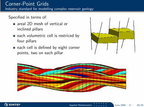
Corner-Point GridsIndustry standard for modelling complex reservoir geology
Specified in terms of:
areal 2D mesh of vertical orinclined pillars
each volumetric cell is restriced byfour pillars
each cell is defined by eight cornerpoints, two on each pillar
Applied Mathematics June 2006 20/30
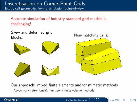
Discretisation on Corner-Point GridsExotic cell geometries from a simulation point-of-view
Accurate simulation of industry-standard grid models ischallenging!
Skew and deformed gridblocks:
Non-matching cells:
Our approach: mixed finite elements and/or mimetic methodsI. Aavatsmark (after lunch): multipoint finite-volume methods
Applied Mathematics June 2006 21/30
Discretisation on General Subgrids
Can use standard mixed FEM for many geometries providedthat one has
mappings (Piola transforms)reference elements
Subdivision of corner-point cells into tetrahedra
Mimetic finite differences (recent work by Brezzi, Lipnikov,Shashkov, Simoncini)
Applied Mathematics June 2006 22/30
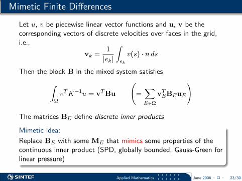
Mimetic Finite Differences
Let u, v be piecewise linear vector functions and u, v be thecorresponding vectors of discrete velocities over faces in the grid,i.e.,
vk =1
|ek|
∫ek
v(s) · nds
Then the block B in the mixed system satisfies∫ΩvTK−1u = vTBu
(=∑E∈Ω
vTEBEuE
)
The matrices BE define discrete inner products
Mimetic idea:
Replace BE with some ME that mimics some properties of thecontinuous inner product (SPD, globally bounded, Gauss-Green forlinear pressure)
Applied Mathematics June 2006 23/30
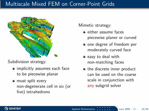
Multiscale Mixed FEM on Corner-Point Grids
Subdivision strategy:
implicitly assumes each faceto be piecewise planar
must split everynon-degenerate cell in six (orfive) tetrahedrons
Mimetic strategy:
either assume facespiecewise planer or curved
one degree of freedom permoderately curved face
easy to deal withnon-matching faces
the discrete inner productcan be used on the coarsescale in conjunction withany subgrid solver
Applied Mathematics June 2006 24/30
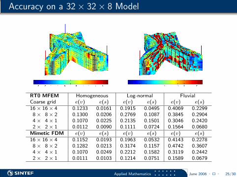
Accuracy on a 32× 32× 8 Model
RT0 MFEM Homogeneous Log-normal FluvialCoarse grid e(v) e(s) e(v) e(s) e(v) e(s)16× 16× 4 0.1233 0.0161 0.1915 0.0495 0.4069 0.22998× 8× 2 0.1300 0.0206 0.2769 0.1087 0.3845 0.29044× 4× 1 0.1070 0.0225 0.2135 0.1501 0.3046 0.24202× 2× 1 0.0112 0.0090 0.1111 0.0724 0.1564 0.0680
Mimetic FDM e(v) e(s) e(v) e(s) e(v) e(s)16× 16× 4 0.1152 0.0193 0.1963 0.0532 0.4143 0.22788× 8× 2 0.1282 0.0213 0.3174 0.1157 0.4742 0.36074× 4× 1 0.1070 0.0249 0.2212 0.1582 0.3119 0.24422× 2× 1 0.0111 0.0103 0.1214 0.0751 0.1589 0.0679
Applied Mathematics June 2006 25/30
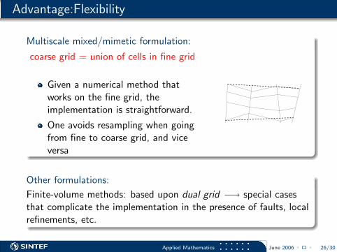
Advantage:Flexibility
Multiscale mixed/mimetic formulation:
coarse grid = union of cells in fine grid
Given a numerical method thatworks on the fine grid, theimplementation is straightforward.
One avoids resampling when goingfrom fine to coarse grid, and viceversa
Other formulations:
Finite-volume methods: based upon dual grid −→ special casesthat complicate the implementation in the presence of faults, localrefinements, etc.
Applied Mathematics June 2006 26/30
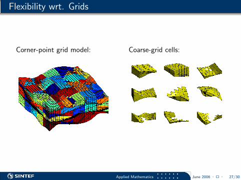
Flexibility wrt. Grids
Corner-point grid model: Coarse-grid cells:
Applied Mathematics June 2006 27/30
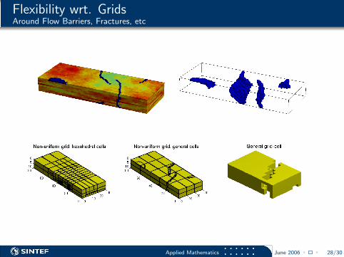
Flexibility wrt. GridsAround Flow Barriers, Fractures, etc
Applied Mathematics June 2006 28/30
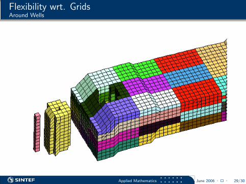
Flexibility wrt. GridsAround Wells
Applied Mathematics June 2006 29/30
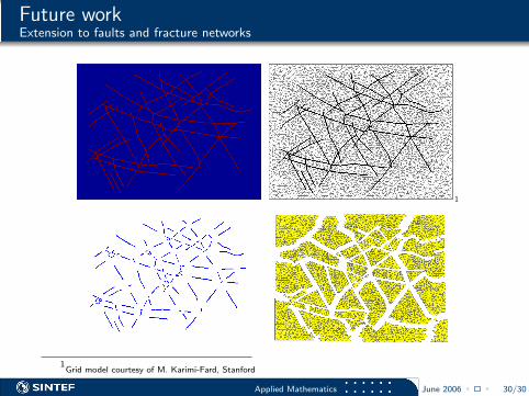
Future workExtension to faults and fracture networks
1
1Grid model courtesy of M. Karimi-Fard, Stanford
Applied Mathematics June 2006 30/30