Multiple Linear Regression(Chapters 12‐13 in 

Montgomery, Runger)

12-1: Multiple Linear Regression Model

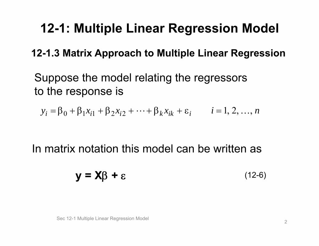
12-1.3 Matrix Approach to Multiple Linear Regression

Suppose the model relating the regressors to the response is

In matrix notation this model can be written as

y = X +

2

nixxxy iikkiii ,,2,122110

Sec 12-1 Multiple Linear Regression Model

(12-6)

12-1: Multiple Linear Regression Model

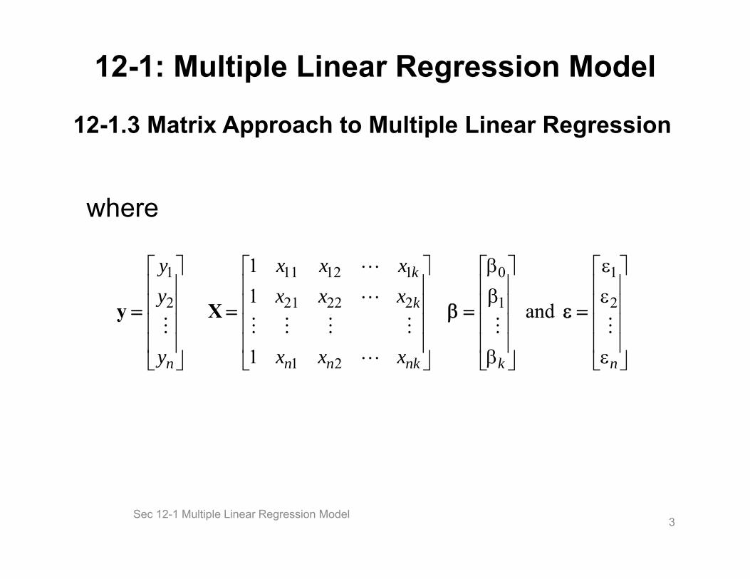
12-1.3 Matrix Approach to Multiple Linear Regression

where

3

nknknn

k

k

n xxx

xxxxxx

y

yy

2

1

1

0

21

22221

11211

2

1

and

1

11

Xy

Sec 12-1 Multiple Linear Regression Model

12-1.3 Matrix Approach to Multiple Linear Regression

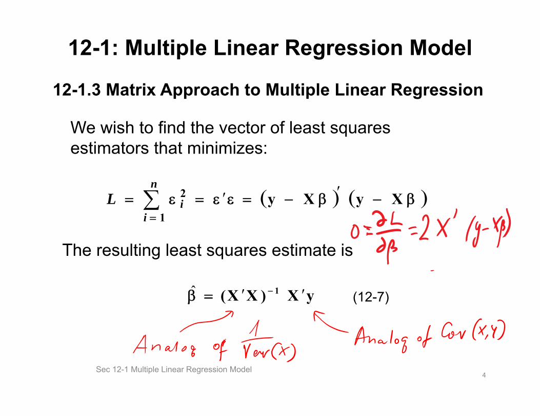
We wish to find the vector of least squares estimators that minimizes:

The resulting least squares estimate is

4

XyXy1

2 n

iiL

ˆ 1(X X ) X y (12-7)

12-1: Multiple Linear Regression Model

Sec 12-1 Multiple Linear Regression Model

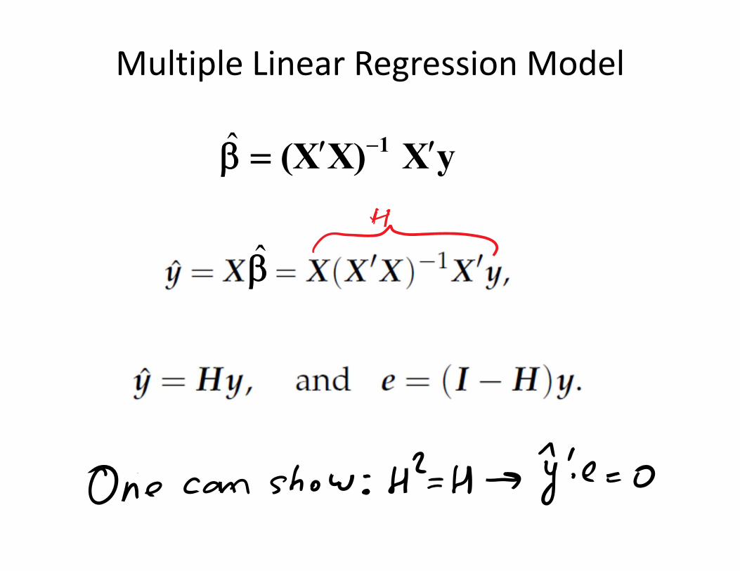
Multiple Linear Regression Model

ˆ 1(X X) X y

12‐1: Multiple Linear Regression Models

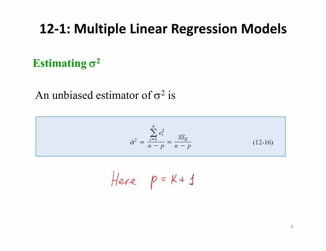
Estimating 2

An unbiased estimator of 2 is

6

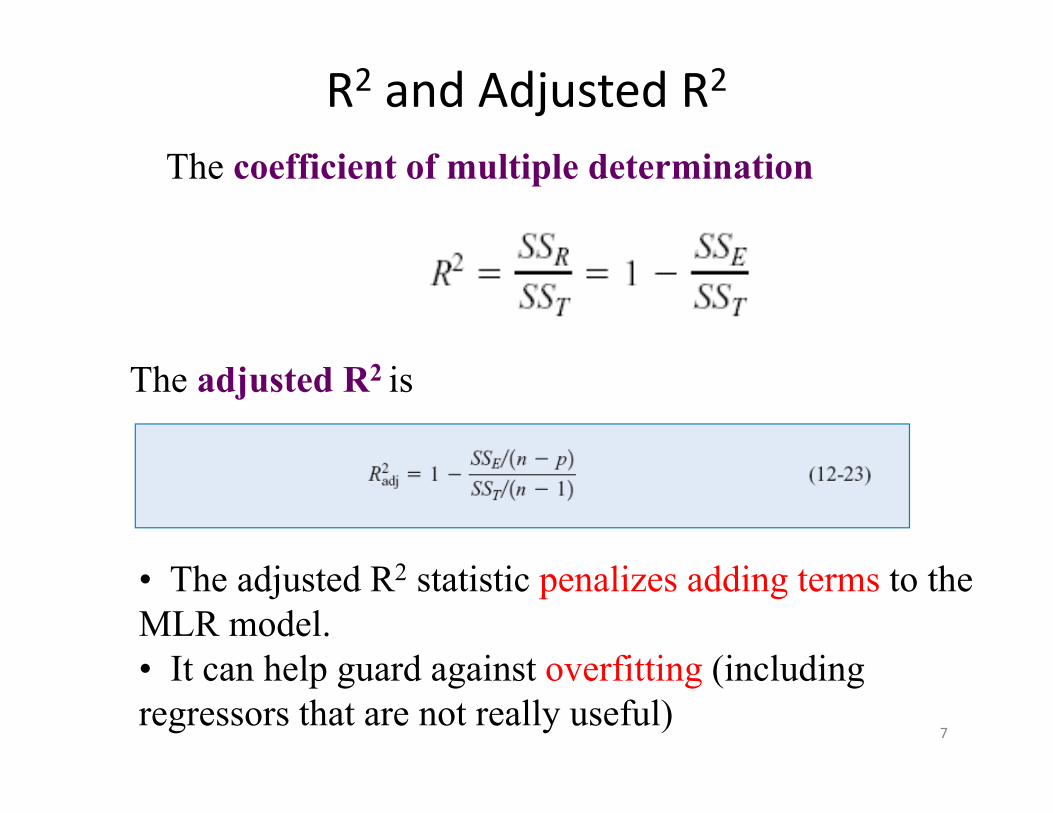
The adjusted R2 is

• The adjusted R2 statistic penalizes adding terms to the MLR model.• It can help guard against overfitting (including regressors that are not really useful)

7

R2 and Adjusted R2

The coefficient of multiple determination

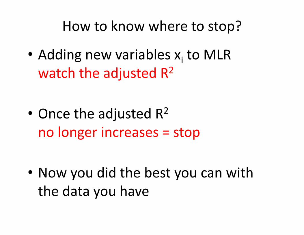
How to know where to stop?

• Adding new variables xi to MLR watch the adjusted R2

• Once the adjusted R2

no longer increases = stop 

• Now you did the best you can with the data you have

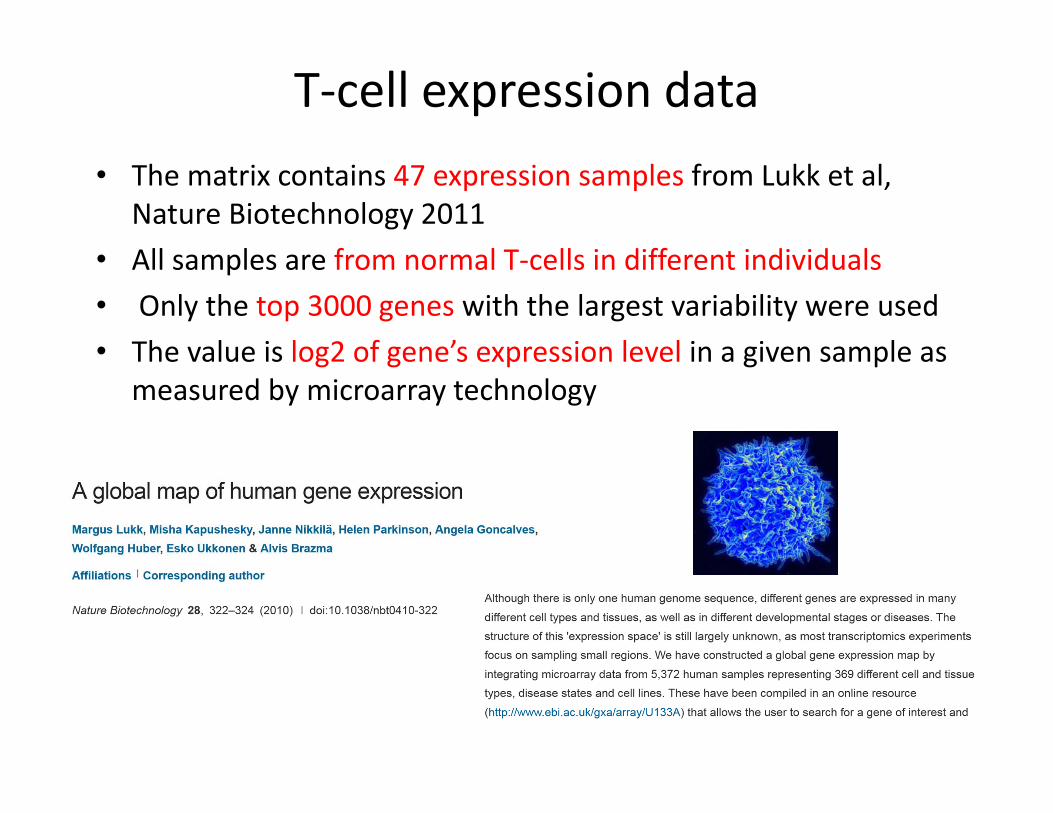
T‐cell expression data• The matrix contains 47 expression samples from Lukk et al, 

Nature Biotechnology 2011• All samples are from normal T‐cells in different individuals• Only the top 3000 genes with the largest variability were used• The value is log2 of gene’s expression level in a given sample as 

measured by microarray technology

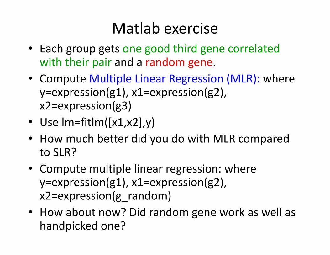
Matlab exercise• Each group gets one good third gene correlated with their pair and a random gene. 

• Compute Multiple Linear Regression (MLR): where y=expression(g1), x1=expression(g2), x2=expression(g3)

• Use lm=fitlm([x1,x2],y)• How much better did you do with MLR compared to SLR? 

• Compute multiple linear regression: where y=expression(g1), x1=expression(g2), x2=expression(g_random)

• How about now? Did random gene work as well as handpicked one?

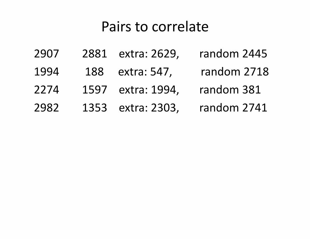
Pairs to correlate

2907        2881    extra: 2629,       random 24451994         188     extra: 547,          random 27182274        1597    extra: 1994,       random 3812982        1353    extra: 2303,       random 2741

Multiple linear regression• load expression_table.mat• % Single variable regression• g1=2907; g2=2881;• y=exp_t(g1,:)'; x=exp_t(g2,:)'• figure; plot(x,y,'ko')• lm=fitlm(x,y)• y_fit=lm.Fitted;• hold on;• plot(x,lm.Fitted,'r‐');

• %Multiple regression• g1=2907; g2=2881; g3=2629;• y=exp_t(g1,:)'; x=[exp_t(g2,:)', exp_t(g3,:)'];• figure; plot(x(:,1),y,'ko');• %figure; plot3(x(:,1),x(:,2),y,'ko');• lm=fitlm(x,y)• y_fit=lm.Fitted;• hold on; plot(x(:,1),y_fit,'rd');

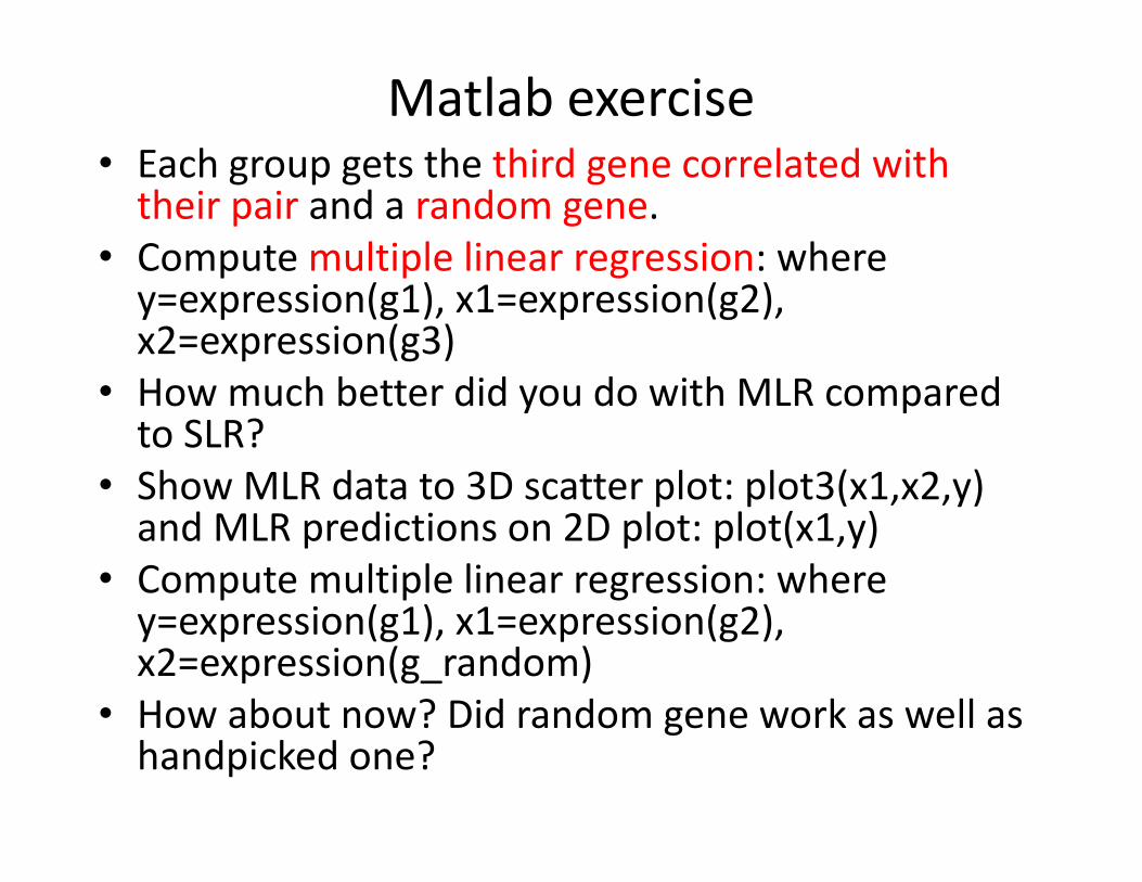
Matlab exercise• Each group gets the third gene correlated with their pair and a random gene. 

• Compute multiple linear regression: where y=expression(g1), x1=expression(g2), x2=expression(g3)

• How much better did you do with MLR compared to SLR? 

• Show MLR data to 3D scatter plot: plot3(x1,x2,y) and MLR predictions on 2D plot: plot(x1,y)

• Compute multiple linear regression: where y=expression(g1), x1=expression(g2), x2=expression(g_random)

• How about now? Did random gene work as well as handpicked one?

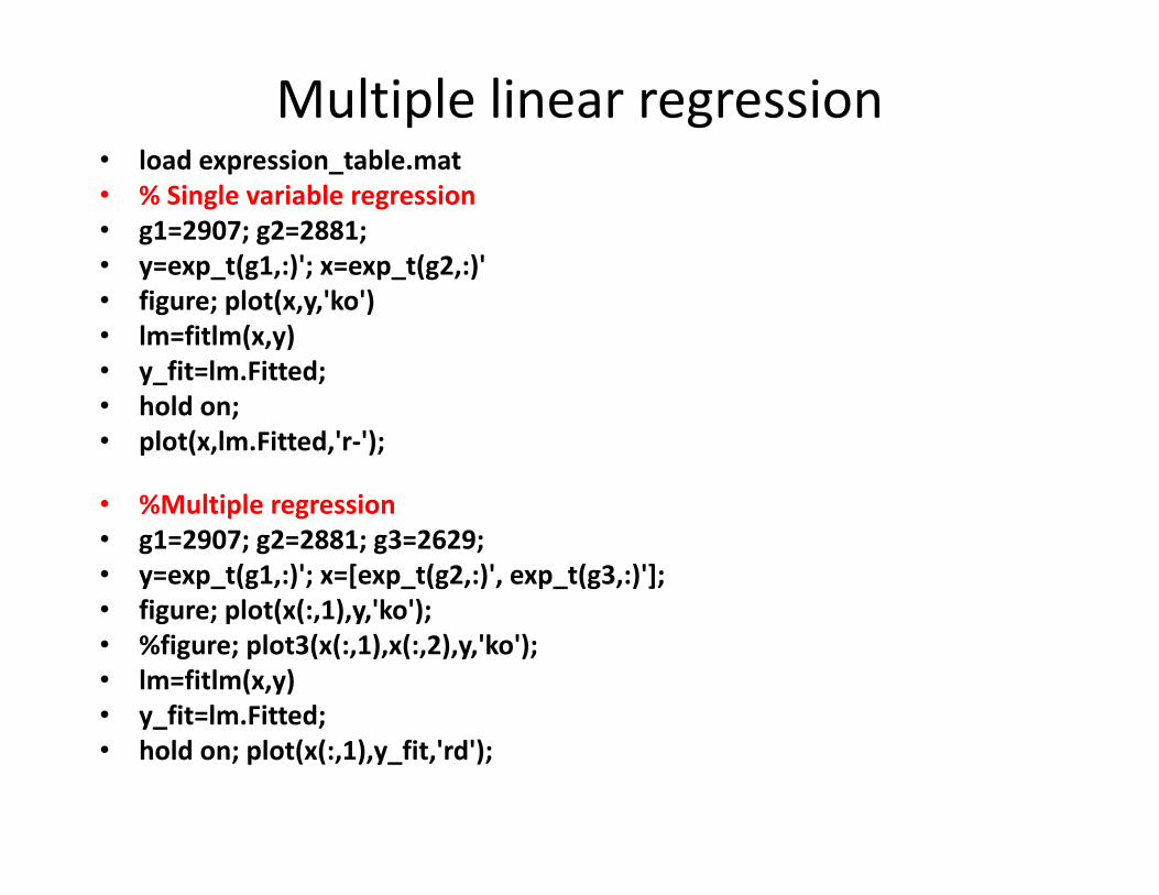
Multiple linear regression• load expression_table.mat• % Single variable regression• g1=2907; g2=2881;• y=exp_t(g1,:)'; x=exp_t(g2,:)'• figure; plot(x,y,'ko')• lm=fitlm(x,y)• y_fit=lm.Fitted;• hold on;• plot(x,lm.Fitted,'r‐');

• %Multiple regression• g1=2907; g2=2881; g3=2629;• y=exp_t(g1,:)'; x=[exp_t(g2,:)', exp_t(g3,:)'];• figure; plot(x(:,1),y,'ko');• %figure; plot3(x(:,1),x(:,2),y,'ko');• lm=fitlm(x,y)• y_fit=lm.Fitted;• hold on; plot(x(:,1),y_fit,'rd');

Clustering analysisof gene expression data

Chapter 11 in Jonathan Pevsner, 

Bioinformatics and Functional Genomics, 3rd edition

(Chapter 9 in 2nd edition)

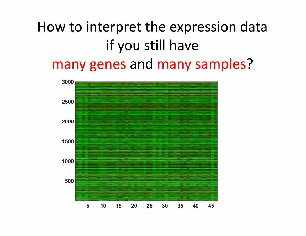
How to interpret the expression data if you still have 

many genes and many samples? 

Clustering to the rescue!

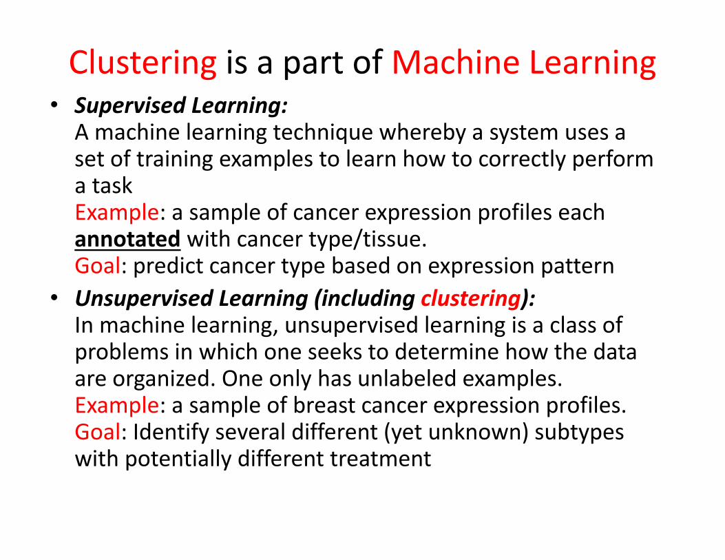
Clustering is a part of Machine Learning• Supervised Learning: 

A machine learning technique whereby a system uses a set of training examples to learn how to correctly perform a taskExample: a sample of cancer expression profiles each annotated with cancer type/tissue. Goal: predict cancer type based on expression pattern 

• Unsupervised Learning (including clustering): In machine learning, unsupervised learning is a class of problems in which one seeks to determine how the data are organized. One only has unlabeled examples. Example: a sample of breast cancer expression profiles. Goal: Identify several different (yet unknown) subtypes with potentially different treatment

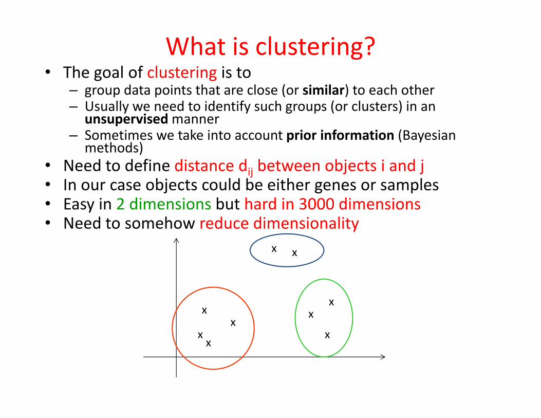
What is clustering?• The goal of clustering is to

– group data points that are close (or similar) to each other– Usually we need to identify such groups (or clusters) in an 

unsupervisedmanner– Sometimes we take into account prior information (Bayesian 

methods)• Need to define distance dij between objects i and j• In our case objects could be either genes or samples• Easy in 2 dimensions but hard in 3000 dimensions• Need to somehow reduce dimensionality

xx

xx

xx

xx

x

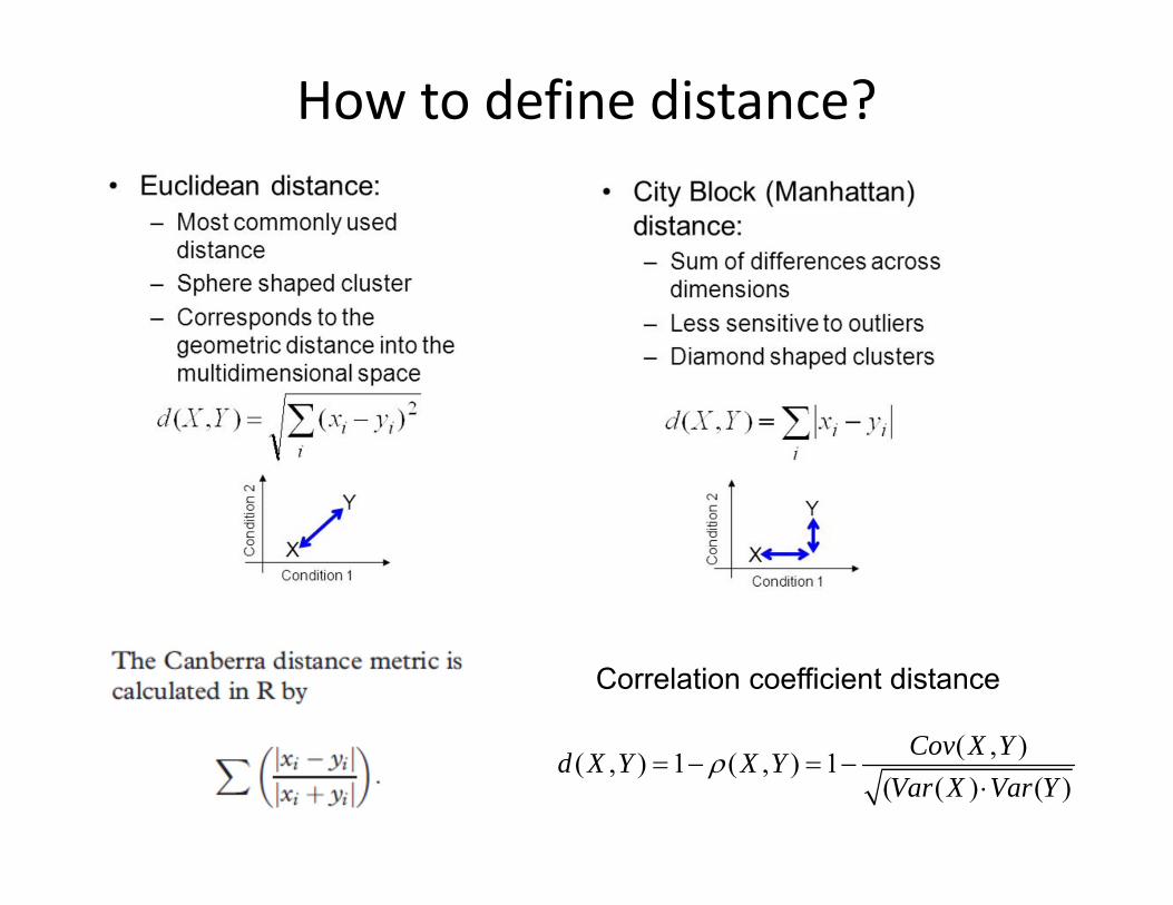
How to define distance?

( , )( , ) 1 ( , ) 1( ( ) ( )

Cov X Yd X Y X YVar X Var Y

Correlation coefficient distance

Reminder:Principal Component Analysis

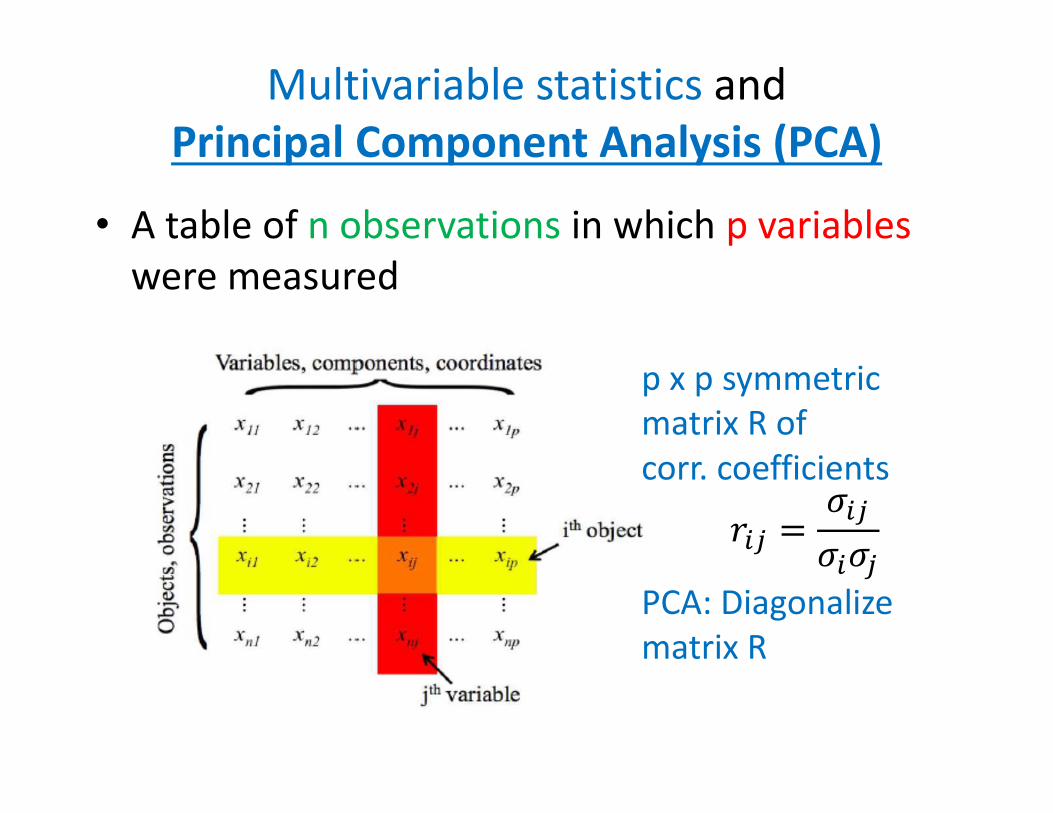
Multivariable statistics and Principal Component Analysis (PCA)

• A table of n observations in which p variables were measured 

p x p symmetric matrix R of corr. coefficients

PCA: Diagonalizematrix R

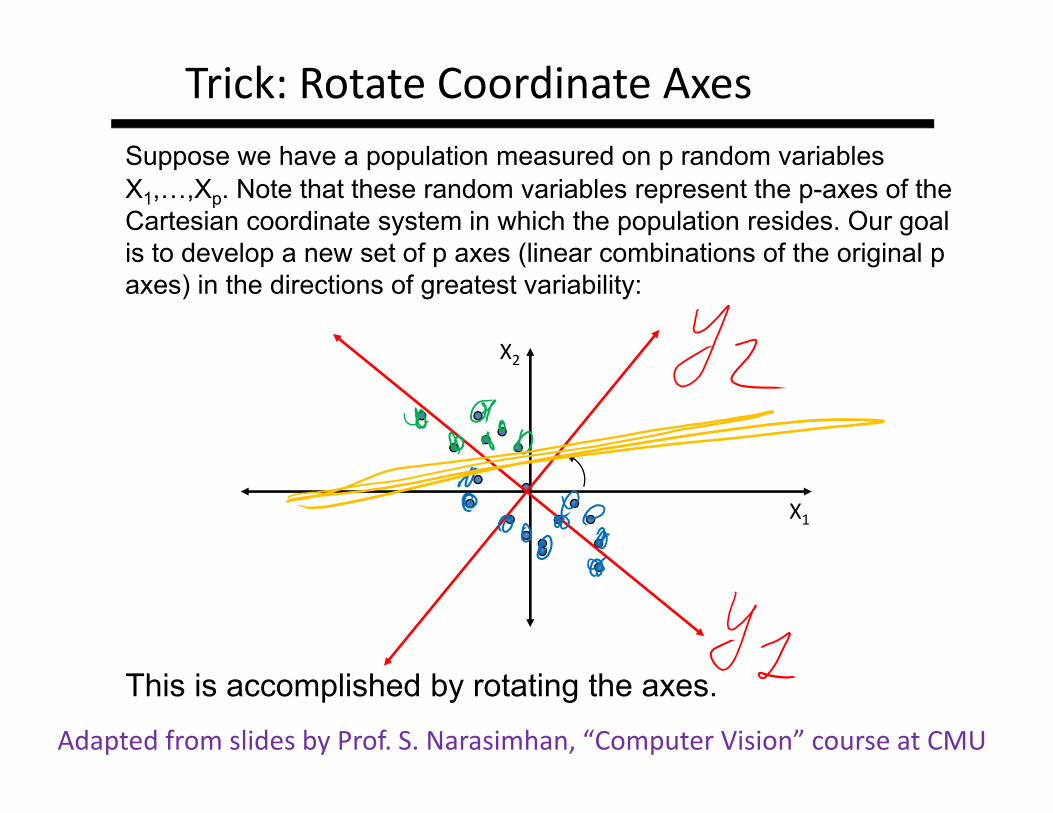
Suppose we have a population measured on p random variables X1,…,Xp. Note that these random variables represent the p-axes of the Cartesian coordinate system in which the population resides. Our goal is to develop a new set of p axes (linear combinations of the original p axes) in the directions of greatest variability:

This is accomplished by rotating the axes.

X1

X2

Trick: Rotate Coordinate Axes

Adapted from slides by Prof. S. Narasimhan, “Computer Vision” course at CMU

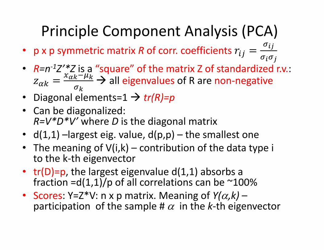
Principle Component Analysis (PCA)• p x p symmetric matrix R of corr. coefficients

• R=n‐1Z’*Z is a “square” of the matrix Z of standardized r.v.:  all eigenvalues of R are non‐negative

• Diagonal elements=1  tr(R)=p• Can be diagonalized: 

R=V*D*V’ where D is the diagonal matrix• d(1,1) –largest eig. value, d(p,p) – the smallest one• The meaning of V(i,k) – contribution of the data type i 

to the k‐th eigenvector • tr(D)=p, the largest eigenvalue d(1,1) absorbs a 

fraction =d(1,1)/p of all correlations can be ~100%• Scores: Y=Z*V: n x p matrix. Meaning of Y(,k) –

participation  of the sample #  in the k‐th eigenvector

Back to clustering

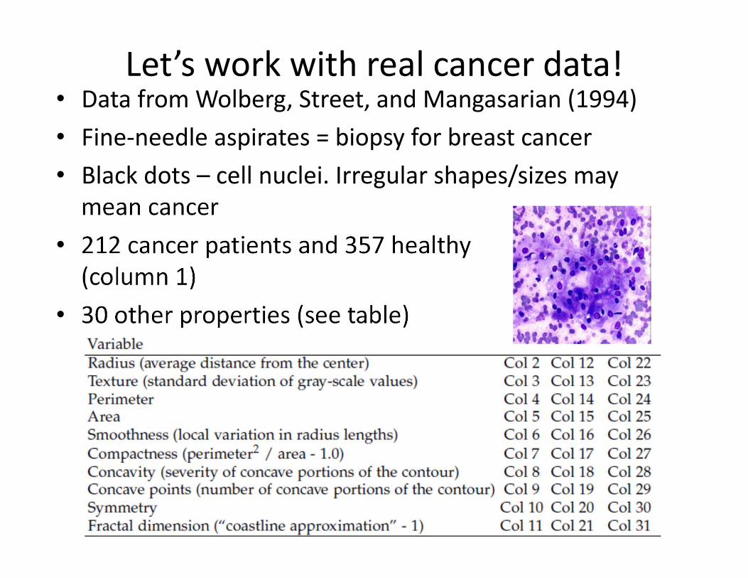
Let’s work with real cancer data!• Data from Wolberg, Street, and Mangasarian (1994) • Fine‐needle aspirates = biopsy for breast cancer • Black dots – cell nuclei. Irregular shapes/sizes may mean cancer

• 212 cancer patients and 357 healthy (column 1)

• 30 other properties (see table)

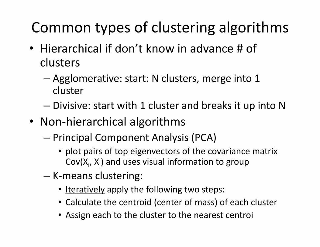
Common types of clustering algorithms• Hierarchical if don’t know in advance # of clusters– Agglomerative: start: N clusters, merge into 1 cluster

– Divisive: start with 1 cluster and breaks it up into N• Non‐hierarchical algorithms

– Principal Component Analysis (PCA)• plot pairs of top eigenvectors of the covariance matrix Cov(Xi, Xj) and uses visual information to group

– K‐means clustering: • Iteratively apply the following two steps:• Calculate the centroid (center of mass) of each cluster • Assign each to the cluster to the nearest centroi

UPGMA algorithm

• Hierarchical agglomerative clustering algorithm• UPGMA = Unweighted Pair Group Method with Arithmetic mean

• Iterative algorithm:• Start with a pair with the smallest d(X,Y)• Cluster these two together and replace it with their arithmetic mean (X+Y)/2

• Recalculate all distances to this new “cluster node”

• Repeat until all nodes are merged

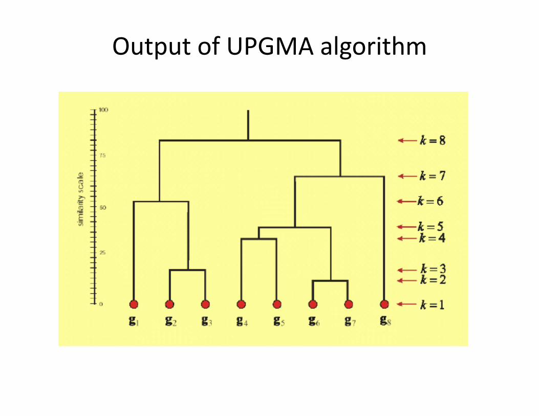
Output of UPGMA algorithm

Credit: XKCD comics 

Matlab demo

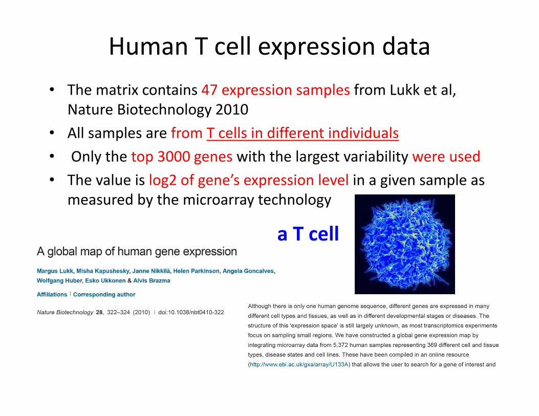
Human T cell expression data• The matrix contains 47 expression samples from Lukk et al, 

Nature Biotechnology 2010• All samples are from T cells in different individuals• Only the top 3000 genes with the largest variability were used• The value is log2 of gene’s expression level in a given sample as 

measured by the microarray technology

• T cellsa T cell 

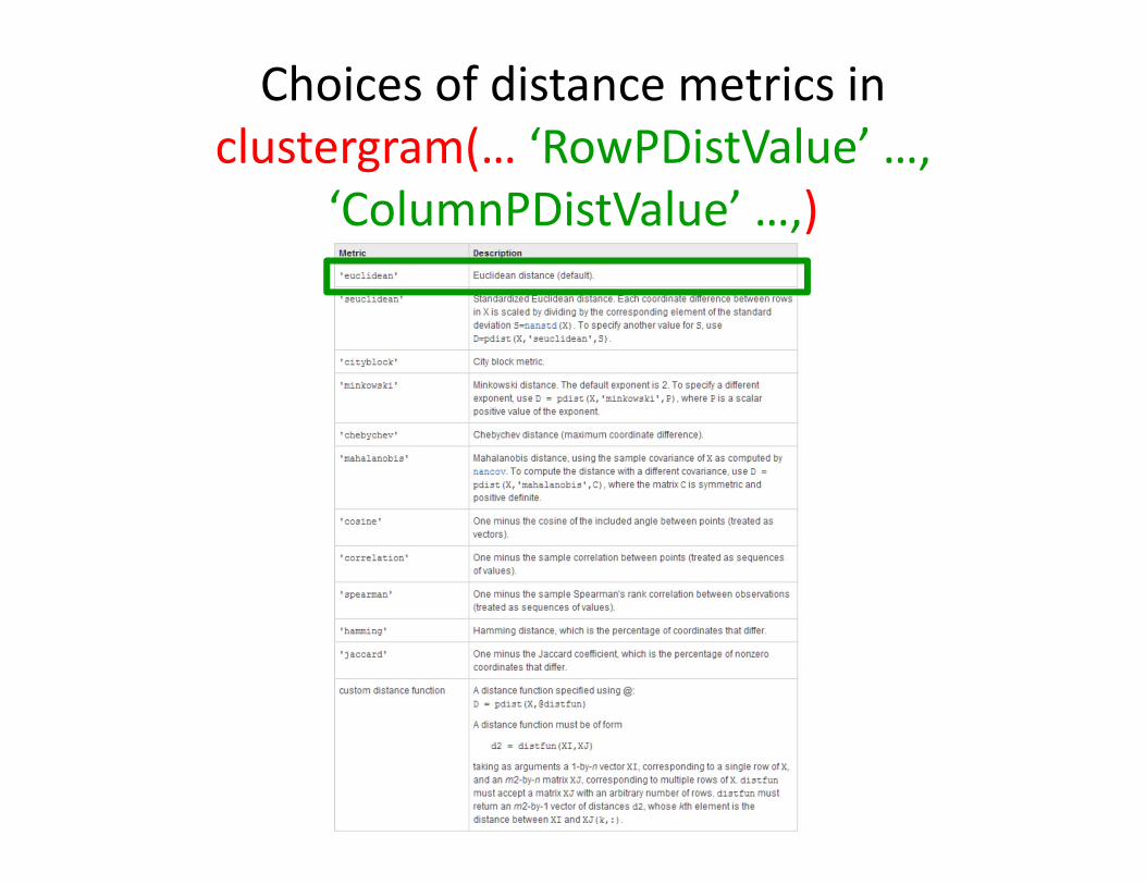
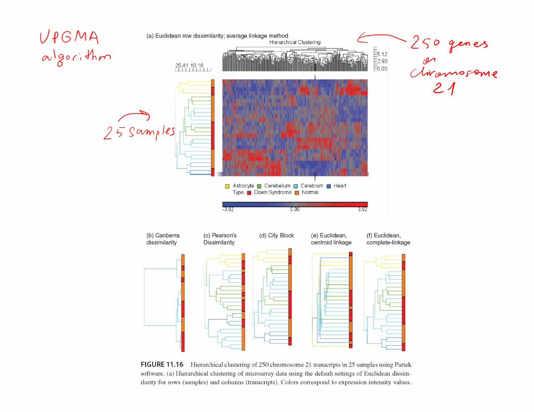
Choices of distance metrics in clustergram(… ‘RowPDistValue’ …,

‘ColumnPDistValue’ …,) 

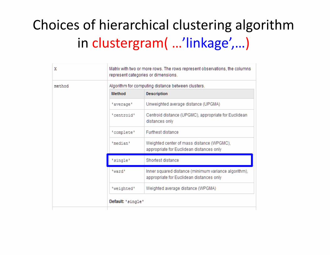
Choices of hierarchical clustering algorithm in clustergram( …’linkage’,…)