©2005, Rajan et. al. 1

Multiphysics CAD-Based Design Optimization

A. Vaidya*, S. Yang† and J. St. Ville‡ Hawthorne & York, Intl, Phoenix, AZ 85008

D. T. Nguyen§ Old Dominion University, Norfolk, VA 23529

S. D. Rajan** Arizona State University, Tempe, AZ 85287

Reducing design cycle time is still remains an important research (and industrial) goal. An integrated model building, finite element analysis (FEA) and design optimization (DO) system increases throughput, reduces errors and makes it easier to maintain the software system. In this paper, we examine how a commercial CAD system can be combined with a finite-element based design optimization system to yield to tightly integrated design system. This design system is then used in sequential and distributed processing computing environments to obtain design optimization solutions of multiphysics problems.

I. Introduction Finite-element based design optimization is now a relatively well-established methodology for engineering design. The use of this methodology involves several areas and techniques such as geometric modeling, mesh generation, finite element analysis, numerical optimization techniques etc. Advances in each of these areas have made the overall design process more versatile especially when and where there is a tight integration between these areas. This integration enables an end-to-end solution with reduced designer intervention. Yet there remain more challenges to meet and hurdles to overcome. As finite element models have become more sophisticated and detailed, the execution time has also increased in spite of advances in hardware technology. Compressing the design cycle time so as to reduce the time required for design and redesign process, requires more advances in hardware, software and algorithms. Structural optimization can be broadly classified into topology, shape and sizing optimization. Topology optimization is used to generate conceptual designs for specified loads and boundary conditions inside a specific design space. Sizing optimization involves the modification of the cross section or thickness of structural elements to obtain an optimum objective function (minimum weight, maximum stiffness, etc.) while satisfying constraints (stress, displacement,

* Product Design Tools Software Engineer † FEA Software Engineer ‡ President § Professor, Civil & Environmental Engineering ** Professor, Civil & Environmental Engineering

©2005, Rajan et. al. 2

etc.). Similarly, shape optimization involves the modification of the parameters that control the shape of the model. Shape optimization in particular can be classified into parametric and non-parametric approaches. Parametric shape optimization necessitates tight integration and full associativity between a CAD solid model and the FEA model. Any changes to the solid model - a perturbation in a linear dimension should result in a corresponding update in the FE model. Such an association makes it possible to use any parameter in the solid model as a design variable in shape optimization process. The biggest advantage of this approach is that at the end of the design process, the designer obtains the final dimensions of the solid model directly making it possible to use the model information in downstream applications such as manufacturability analyses or process planning. Additionally, this approach ensures that the geometry stays consistent, i.e. a straight line remains a straight line, slope continuity is retained and enforced etc. However, this approach requires careful model building. Boundary conditions and loads must be prescribed on the geometry and not directly on the FE model. The solid model geometry must be parameterized carefully to ensure behavior consistent with the designer’s intent. Finally, in all parametric based shape optimization, changes in design variables result in a regeneration of the FE mesh and this significantly increases computation time for large meshes and large numbers of design variables. Non-parametric shape optimization on the other hand works directly on the finite element model. Users specify the shape variables by selecting FE nodes and specifying how the changes in the nodal coordinates are to take place. There are advantages to this approach. First, the mesh stays the same (number of nodes and elements does not change) leading to a smoother convergence. Second, no special action needs to take place with the specification of loads and boundary conditions. Third, the geometric or solider modeler and the mesh generator are not invoked during the shape changes. The biggest challenge is to ensure that mesh distortion is postponed as much as possible since recreation of the model (after mesh distortion) necessitates user interaction. In addition, unless special action is taken, it may be quite difficult for the designer to specify shape changes that stay consistent with the original design intent, e.g. ensuring curvature continuity so that it can be machined easily. Finally, there is the problem of taking the final results and recreating the solid model for effective use by a downstream application. The main aim of design optimization is to reduce the design cycle time to increase the efficiency of the overall process. There are many commercial and research systems that perform various stages of structural optimization. Spath et. al.1 concentrate mainly on topology optimization and use TOSCA and MSC.Construct for that purpose. A mesh smoothing procedure is used to reduce the amount of data to be imported into a CAD system from the results of topology optimization. Standard formats such as Initial Graphics Exchange Specifications (IGES) or Stereo Lithography (STL) files are used to import the model into a CAD system potentially for further shape optimization or other downstream activities in the design process. For example, a commercial product GENESIS from VRand2,3,4,5 links an optimizer with another commercial modeling system, SDRC-IDEAS. This system is then used for topology optimization followed by sizing optimization of composites commonly found in automobile applications3. Results from topology optimization are interpreted visually and used to create a finite element model using IDEAS2,4. For shape optimization, non-structural regions termed DOMAINS5 are manually created using

©2005, Rajan et. al. 3

the FE model and mesh smoothing is used to prevent mesh distortion. There have been other examples of integration of two different software systems. Meske et. al.6, 7 use ABAQUS for finite element analysis and TOSCA for topology/non-parametric shape optimization of non-linear and contact problems. As before, the topology results from TOSCA are exported as an STL or IGES file to be imported into a CAD system while for shape optimization, the user manually creates node sets or groups directly on the FE model so that shape changes are possible. In another example Nima et. al.8 use an optimization kernel called CAOSS and MSC/NASTRAN. Since TOSCA is based on CAOSS6, the approach used for non-parametric shape optimization is quite similar using local nodes and local nodal strains as the inputs for shape optimization. The shape optimizer uses an adaptive mesh correction algorithm to prevent mesh distortion. Dirschmid9 uses MSC/CONSTRUCT and MSC/NASTRAN for topology followed by non-parametric shape optimization and/or sizing optimization of automotive components. Once again for the shape optimization, nodal displacements and couplings are used to define the data necessary for shape optimization. ANSYS supplies a module called Workbench10 for parametric shape optimization that is associated directly with various CAD systems11. In this sense it is similar to Unigraphics NX Optimization Wizard12 and relies on re-meshing the model while perturbing parameters and performing shape optimization. Another commercial product that integrates topology and non-parametric shape optimization is Optistruct13. While much work has taken place in carrying out the various design optimization stages, the critical issues such as tight end-to-end integration still is a big challenge. How does the designer create the design information (topology, shape and sizing) using the solid modeler? How can the results obtained by topology optimization be moved to a finite element model that can be used for sizing and shape optimization in such a manner that the overall design cycle time is reduced? While some of the systems discussed earlier use standard formats like STL to import topology optimization results into a CAD system, it should be noted that STL data cannot be directly converted into boundary representation data. Thus, the user may have to manually create a solid model followed by an FE model that is based on the solid model. Any change in the mesh will make it necessary to go through the whole procedure once again. This paper proposes parametric shape optimization approach that is based on the Hybrid Natural Approach14,15. The key point is to enable a user to perform parametric shape optimization with as little re-meshing as possible. The parametric approach also ensures that the designer will have a CAD solid model representation of the optimized design having the same geometric characteristics as the original design. To ensure that the results are accurate, some re-meshing is inevitable if significant changes take place during the optimization. However, reducing the time for re-meshing has significant computational benefits that will only increase as the FE model size increases. In this paper, we present our approach to creating a design engineering workbench. The FE model building takes place using Unigraphics NX 3 (UG). Design model is created using our own preprocessor. The preliminary design optimization takes place using the single processor desktop system. The detailed design takes place on a relatively small computing cluster. Finally the design results are translated back and incorporated into the UG geometric model.

©2005, Rajan et. al. 4

II. Design Optimization Methodology Most single objective design optimization problems can be formulated as follows.

Find kR∈x (1a) To minimize ( )f x (1b) Subject to ( ) 0 1,2,...,ig i m≤ =x (1c) , 1, 2,...,L U

j j jx x x j k≤ ≤ = (1d) Typically, this problem is solved using a gradient-based technique. Among gradient-based methods, Method of Feasible Directions (used in this paper), Generalized Reduced Gradient and Sequential Quadratic Programming are the most popular. In a typical sequential algorithm there are eight steps.

(1) Carry out a function evaluation with the initial guess. (2) Start design iterations. (3) Carry out gradient evaluation at current design point. (4) Solve direction-finding problem. (5) Find optimal step length from line search problem. (6) Compute the next design point. (7) Converged solution? If “no”, go to step 3. (8) If “yes”, carry out the final function evaluation with the optimal values. There has been

considerable attention paid to coarse-grain, single level parallelization of optimization algorithms.

We will briefly examine how we have parallelized the various DO steps.

A. Parallel Gradient Evaluation (GE) Gradients are evaluated using the forward difference method. For example, the derivative of a function ( )f x with respect to the ith design variable is given by

( ) ( ) ( )1 2 1 2 1 2, ,... , ,... ,... , ,...n i i n n

i i

f x x x f x x x x x f x x xx x

∂ + ∆ −=

∂ ∆ (2)

The number of FE analyses required during gradient evaluation is equal to the number of design variables. When multiple processors are available, gradient evaluation can be parallelized such that the number of FEAs is divided equally among the available processes. With this scenario, it is possible to obtain an ideal speedup.

B. Parallel Line Search (LS) Parallel line search is implemented using a combination of the multi-section scheme16 and parallel Avriel search17. Details are omitted here but can be found in the earlier work18. The overall algorithm can be split into three steps. Step 1: Bracketing the minimum In this step, the idea is to bracket the interval whose end points have maximum constraint values of opposite sign. Step 2: Zero-finding Once the minimum has been bracketed, the next step is to find a feasible point that is as close to the constraint surface within the constraint thickness tolerance.

©2005, Rajan et. al. 5

Step 3: Function minimization using parallel Avriel search Finally, using information from Step 2, we can compute the lowest function value ( )i

jf α in parallel until the size of the final uncertainty interval falls below a predefined tolerance value. Both an analysis of the algorithm and numerical experimentation show that a decent speedup is possible with only a few number of processors (between 4 and 16)16.

C. Parallel Direction Finding (DF) It should be noted that in the Method of Feasible Directions, line search involves searching along a direction vector that lies within the usable feasible cone. It is possible to compute more than one search direction and conduct a line search along each of those directions so as to find the best possible solution. Numerical results using MFD show that these parallel DF and LS approaches yield expected speedup19. D. Finite Element Analysis Finally, it is possible to attain speedup during design optimization by carrying out the finite element analysis required during function evaluations in parallel. This speedup is realized only when the FE model is sufficiently large and the condition number of the iterative solver is such that a decent convergence rate is attained19. As we see from these discussions, almost every step in the gradient-based design optimization algorithm can be parallelized.

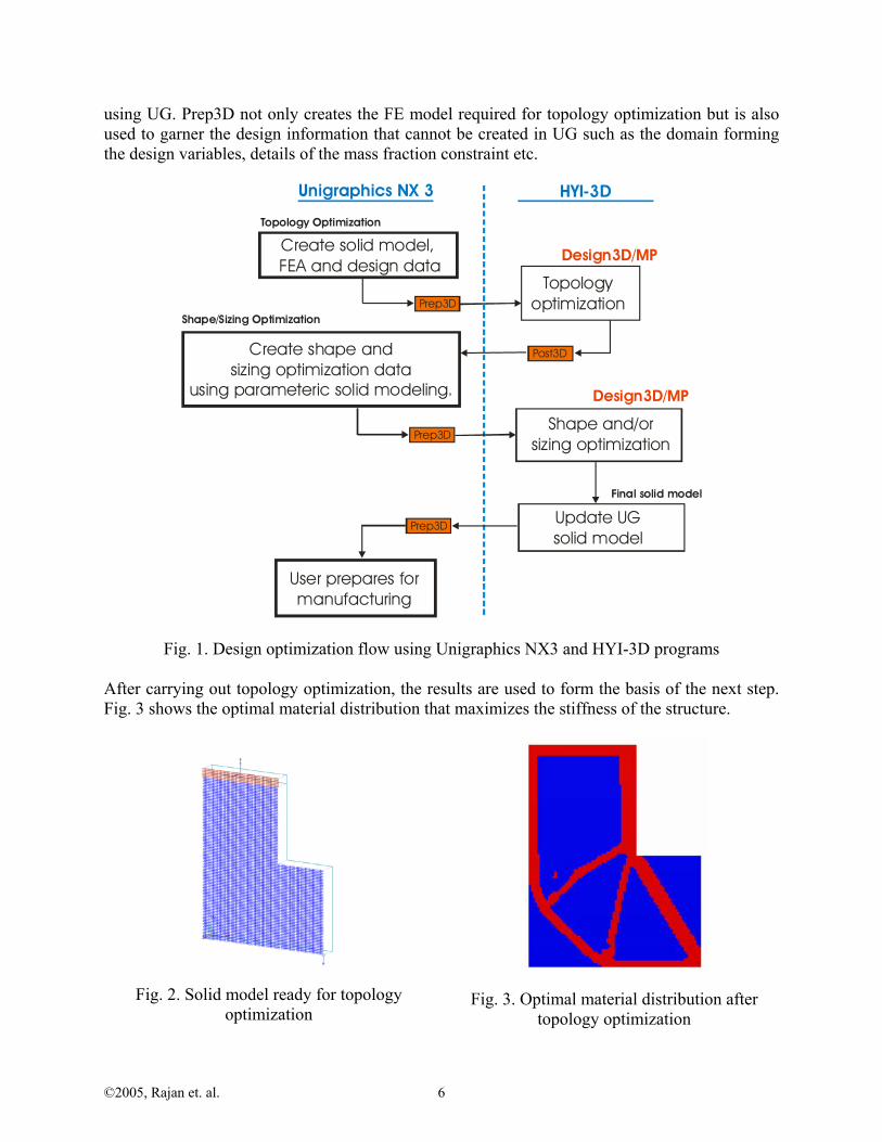
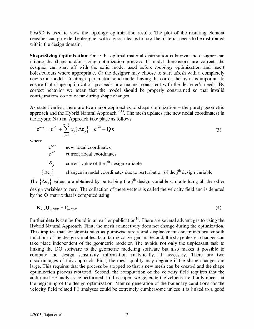
III. Integration with CAD Program In this section we discuss how a reasonably tight integration can be created between the geometric, finite element and the design optimization models. The overall design optimization flow is shown in Fig. 1. HYI-3D20 is developed using object-oriented concepts in C++. The software suite is a collection of independent modules that can be plugged together to create the required set of finite element analysis and design optimization capabilities and can be executed either sequentially (Design3D) or in parallel (Design3DMP) using Message Passing Interface (MPI). Prep3D is the module used to (a) build the HYI-3D FE and DO databases from the UG database and (b) rebuild the UG database (part information) after obtaining the HYI-3D design optimization results. Post3D is a GUI-based module that is used to view FE and DO information graphically. Topology Optimization: A new design optimization problem is usually tackled first as a topology optimization problem. The designer initially creates the problem domain. The boundary of this domain is either stress free, or is subjected to surface tractions, or is supported so as to prevent rigid body modes. It is relatively easy to create the solid model in the modeler. An example (L-bracket19) is shown in Fig. 2. If the SIMP (Simple Isotropic Model with Penalization) or power-law approach is used, it is necessary to indicate which parts of the problem domain are potential design variables and which are not. In Fig. 2, the material in the red zone is not allowed to vary whereas the material in the blue zone forms the potential design variables. The solid model information is then used to create the FE model. This FE model is completely associative with the solid model and thus, any changes in the solid model can be seamlessly transferred to the FE model. In this paper, we create the solid and the FE models

©2005, Rajan et. al. 6

using UG. Prep3D not only creates the FE model required for topology optimization but is also used to garner the design information that cannot be created in UG such as the domain forming the design variables, details of the mass fraction constraint etc.

Create solid model, FEA and design data

Unigraphics NX 3 HYI-3D

Topologyoptimization

Create shape and sizing optimization data

using parameteric solid modeling.

Shape and/orsizing optimization

Update UGsolid model

User prepares formanufacturing

Prep3D

Prep3D

Prep3D

Design3D/MP

Design3D/MP

Post3D

Topology Optimization

Shape/Sizing Optimization

Final solid model

Fig. 1. Design optimization flow using Unigraphics NX3 and HYI-3D programs

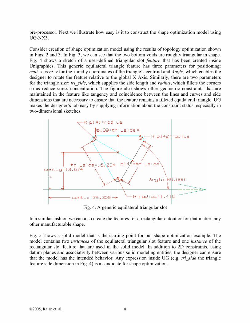
After carrying out topology optimization, the results are used to form the basis of the next step. Fig. 3 shows the optimal material distribution that maximizes the stiffness of the structure.

Fig. 2. Solid model ready for topology optimization

Fig. 3. Optimal material distribution after topology optimization

©2005, Rajan et. al. 7

Post3D is used to view the topology optimization results. The plot of the resulting element densities can provide the designer with a good idea as to how the material needs to be distributed within the design domain. Shape/Sizing Optimization: Once the optimal material distribution is known, the designer can initiate the shape and/or sizing optimization process. If model dimensions are correct, the designer can start off with the solid model used before topology optimization and insert holes/cutouts where appropriate. Or the designer may choose to start afresh with a completely new solid model. Creating a parametric solid model having the correct behavior is important to ensure that shape optimization proceeds in a manner consistent with the designer’s needs. By correct behavior we mean that the model should be properly constrained so that invalid configurations do not occur during shape changes. As stated earlier, there are two major approaches to shape optimization – the purely geometric approach and the Hybrid Natural Approach14,15. The mesh updates (the new nodal coordinates) in the Hybrid Natural Approach take place as follows.

{ }1

NDVnew old old

j jj

x=

= + ∆ = +∑c c c c Qx (3)

where newc new nodal coordinates oldc current nodal coordinates

jx current value of the jth design variable

{ }j∆c changes in nodal coordinates due to perturbation of the jth design variable

The { }j∆c values are obtained by perturbing the jth design variable while holding all the other design variables to zero. The collection of these vectors is called the velocity field and is denoted by the Q matrix that is computed using n n n NDV n NDV× × ×K Q = F (4) Further details can be found in an earlier publication14. There are several advantages to using the Hybrid Natural Approach. First, the mesh connectivity does not change during the optimization. This implies that constraints such as pointwise stress and displacement constraints are smooth functions of the design variables, facilitating convergence. Second, the shape design changes can take place independent of the geometric modeler. The avoids not only the unpleasant task to linking the DO software to the geometric modeling software but also makes it possible to compute the design sensitivity information analytically, if necessary. There are two disadvantages of this approach. First, the mesh quality may degrade if the shape changes are large. This requires that the process be stopped so that a new mesh can be created and the shape optimization process restarted. Second, the computation of the velocity field requires that the additional FE analysis be performed. In this paper, we generate the velocity field only once – at the beginning of the design optimization. Manual generation of the boundary conditions for the velocity field related FE analyses could be extremely cumbersome unless it is linked to a good

©2005, Rajan et. al. 8

pre-processor. Next we illustrate how easy is it to construct the shape optimization model using UG-NX3.

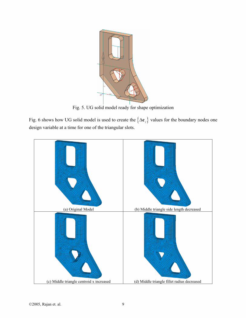
Consider creation of shape optimization model using the results of topology optimization shown in Figs. 2 and 3. In Fig. 3, we can see that the two bottom voids are roughly triangular in shape. Fig. 4 shows a sketch of a user-defined triangular slot feature that has been created inside Unigraphics. This generic equilateral triangle feature has three parameters for positioning: cent_x, cent_y for the x and y coordinates of the triangle’s centroid and Angle, which enables the designer to rotate the feature relative to the global X Axis. Similarly, there are two parameters for the triangle size: tri_side, which supplies the side length and radius, which fillets the corners so as reduce stress concentration. The figure also shows other geometric constraints that are maintained in the feature like tangency and coincidence between the lines and curves and side dimensions that are necessary to ensure that the feature remains a filleted equilateral triangle. UG makes the designer’s job easy by supplying information about the constraint status, especially in two-dimensional sketches.

Fig. 4. A generic equilateral triangular slot

In a similar fashion we can also create the features for a rectangular cutout or for that matter, any other manufacturable shape. Fig. 5 shows a solid model that is the starting point for our shape optimization example. The model contains two instances of the equilateral triangular slot feature and one instance of the rectangular slot feature that are used in the solid model. In addition to 2D constraints, using datum planes and associativity between various solid modeling entities, the designer can ensure that the model has the intended behavior. Any expression inside UG (e.g. tri_side the triangle feature side dimension in Fig. 4) is a candidate for shape optimization.

©2005, Rajan et. al. 9

Fig. 5. UG solid model ready for shape optimization

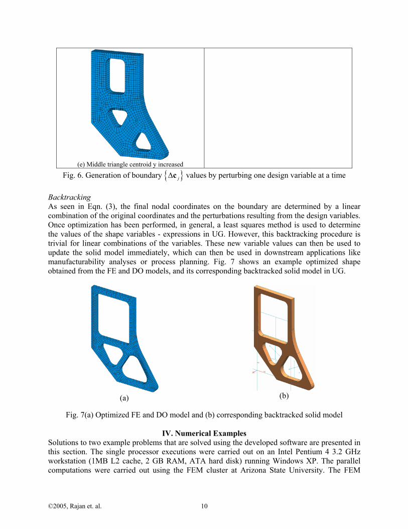
Fig. 6 shows how UG solid model is used to create the { }j∆c values for the boundary nodes one design variable at a time for one of the triangular slots.

(a) Original Model

(b) Middle triangle side length decreased

(c) Middle triangle centroid x increased

(d) Middle triangle fillet radius decreased

©2005, Rajan et. al. 10

(e) Middle triangle centroid y increased

Fig. 6. Generation of boundary { }j∆c values by perturbing one design variable at a time

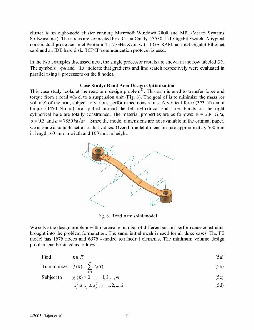
Backtracking As seen in Eqn. (3), the final nodal coordinates on the boundary are determined by a linear combination of the original coordinates and the perturbations resulting from the design variables. Once optimization has been performed, in general, a least squares method is used to determine the values of the shape variables - expressions in UG. However, this backtracking procedure is trivial for linear combinations of the variables. These new variable values can then be used to update the solid model immediately, which can then be used in downstream applications like manufacturability analyses or process planning. Fig. 7 shows an example optimized shape obtained from the FE and DO models, and its corresponding backtracked solid model in UG.

(a)

(b)

Fig. 7(a) Optimized FE and DO model and (b) corresponding backtracked solid model

IV. Numerical Examples

Solutions to two example problems that are solved using the developed software are presented in this section. The single processor executions were carried out on an Intel Pentium 4 3.2 GHz workstation (1MB L2 cache, 2 GB RAM, ATA hard disk) running Windows XP. The parallel computations were carried out using the FEM cluster at Arizona State University. The FEM

©2005, Rajan et. al. 11

cluster is an eight-node cluster running Microsoft Windows 2000 and MPI (Verari Systems Software Inc.). The nodes are connected by a Cisco Catalyst 3550-12T Gigabit Switch. A typical node is dual-processor Intel Pentium 4-1.7 GHz Xeon with 1 GB RAM, an Intel Gigabit Ethernet card and an IDE hard disk. TCP/IP communication protocol is used. In the two examples discussed next, the single processor results are shown in the row labeled SP. The symbols –ge and –ls indicate that gradients and line search respectively were evaluated in parallel using 8 processors on the 8 nodes.

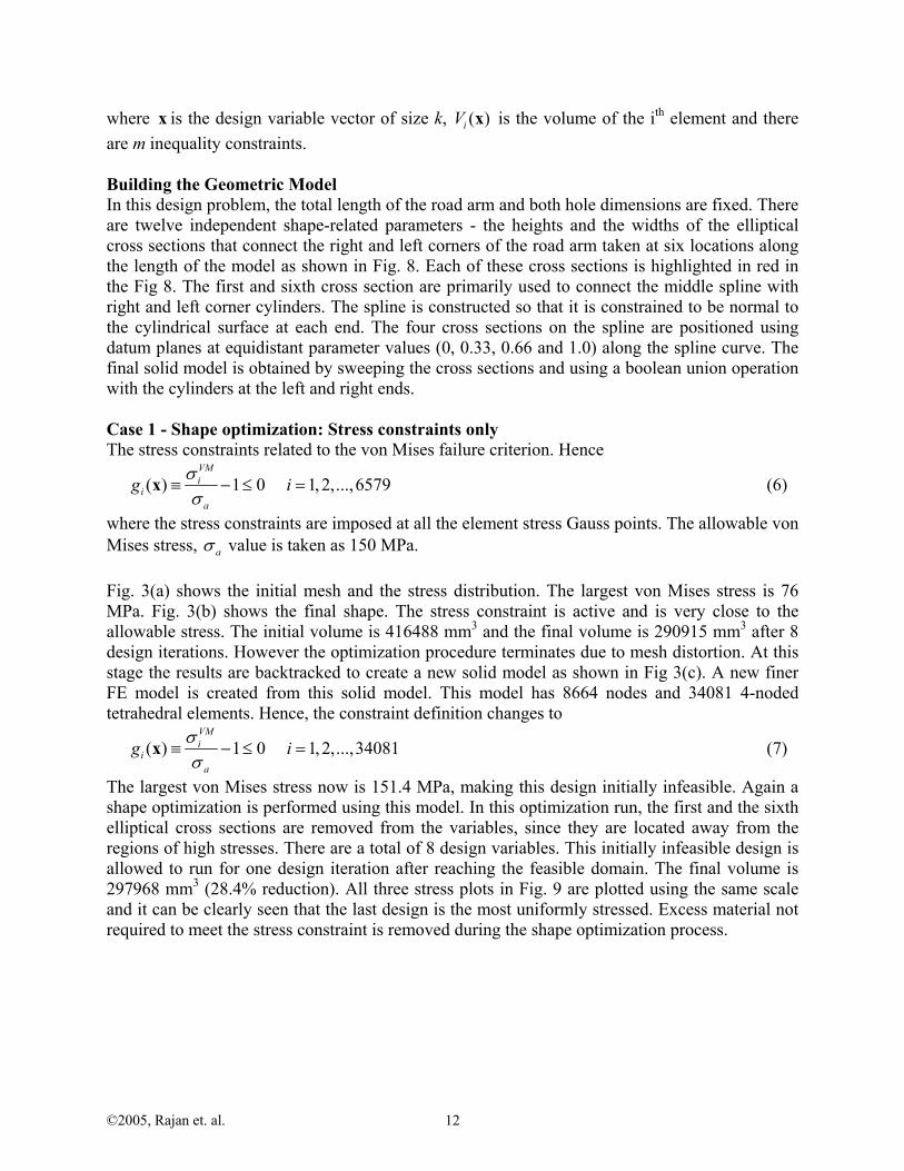
Case Study: Road Arm Design Optimization This case study looks at the road arm design problem21. This arm is used to transfer force and torque from a road wheel to a suspension unit (Fig. 8). The goal of is to minimize the mass (or volume) of the arm, subject to various performance constraints. A vertical force (373 N) and a torque (4450 N-mm) are applied around the left cylindrical end hole. Points on the right cylindrical hole are totally constrained. The material properties are as follows: E = 206 GPa,

0.3υ = and 37850kg mρ = . Since the model dimensions are not available in the original paper, we assume a suitable set of scaled values. Overall model dimensions are approximately 500 mm in length, 60 mm in width and 100 mm in height.

Fig. 8. Road Arm solid model We solve the design problem with increasing number of different sets of performance constraints brought into the problem formulation. The same initial mesh is used for all three cases. The FE model has 1979 nodes and 6579 4-noded tetrahedral elements. The minimum volume design problem can be stated as follows.

Find kR∈x (5a)

To minimize 1

( ) ( )n

ii

f V=

= ∑x x (5b)

Subject to ( ) 0 1,2,...,ig i m≤ =x (5c) , 1, 2,...,L U

j j jx x x j k≤ ≤ = (5d)

©2005, Rajan et. al. 12

where x is the design variable vector of size k, ( )iV x is the volume of the ith element and there are m inequality constraints.

Building the Geometric Model In this design problem, the total length of the road arm and both hole dimensions are fixed. There are twelve independent shape-related parameters - the heights and the widths of the elliptical cross sections that connect the right and left corners of the road arm taken at six locations along the length of the model as shown in Fig. 8. Each of these cross sections is highlighted in red in the Fig 8. The first and sixth cross section are primarily used to connect the middle spline with right and left corner cylinders. The spline is constructed so that it is constrained to be normal to the cylindrical surface at each end. The four cross sections on the spline are positioned using datum planes at equidistant parameter values (0, 0.33, 0.66 and 1.0) along the spline curve. The final solid model is obtained by sweeping the cross sections and using a boolean union operation with the cylinders at the left and right ends. Case 1 - Shape optimization: Stress constraints only The stress constraints related to the von Mises failure criterion. Hence

( ) 1 0 1,2,...,6579VMi

ia

g iσσ

≡ − ≤ =x (6)

where the stress constraints are imposed at all the element stress Gauss points. The allowable von Mises stress, aσ value is taken as 150 MPa. Fig. 3(a) shows the initial mesh and the stress distribution. The largest von Mises stress is 76 MPa. Fig. 3(b) shows the final shape. The stress constraint is active and is very close to the allowable stress. The initial volume is 416488 mm3 and the final volume is 290915 mm3 after 8 design iterations. However the optimization procedure terminates due to mesh distortion. At this stage the results are backtracked to create a new solid model as shown in Fig 3(c). A new finer FE model is created from this solid model. This model has 8664 nodes and 34081 4-noded tetrahedral elements. Hence, the constraint definition changes to

( ) 1 0 1,2,...,34081VMi

ia

g iσσ

≡ − ≤ =x (7)

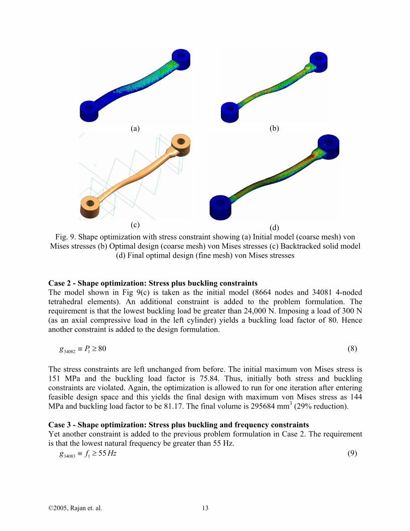
The largest von Mises stress now is 151.4 MPa, making this design initially infeasible. Again a shape optimization is performed using this model. In this optimization run, the first and the sixth elliptical cross sections are removed from the variables, since they are located away from the regions of high stresses. There are a total of 8 design variables. This initially infeasible design is allowed to run for one design iteration after reaching the feasible domain. The final volume is 297968 mm3 (28.4% reduction). All three stress plots in Fig. 9 are plotted using the same scale and it can be clearly seen that the last design is the most uniformly stressed. Excess material not required to meet the stress constraint is removed during the shape optimization process.

©2005, Rajan et. al. 13

(a)

(b)

(c) (d)

Fig. 9. Shape optimization with stress constraint showing (a) Initial model (coarse mesh) von Mises stresses (b) Optimal design (coarse mesh) von Mises stresses (c) Backtracked solid model

(d) Final optimal design (fine mesh) von Mises stresses Case 2 - Shape optimization: Stress plus buckling constraints The model shown in Fig 9(c) is taken as the initial model (8664 nodes and 34081 4-noded tetrahedral elements). An additional constraint is added to the problem formulation. The requirement is that the lowest buckling load be greater than 24,000 N. Imposing a load of 300 N (as an axial compressive load in the left cylinder) yields a buckling load factor of 80. Hence another constraint is added to the design formulation. 34082 1 80g P≡ ≥ (8) The stress constraints are left unchanged from before. The initial maximum von Mises stress is 151 MPa and the buckling load factor is 75.84. Thus, initially both stress and buckling constraints are violated. Again, the optimization is allowed to run for one iteration after entering feasible design space and this yields the final design with maximum von Mises stress as 144 MPa and buckling load factor to be 81.17. The final volume is 295684 mm3 (29% reduction).

Case 3 - Shape optimization: Stress plus buckling and frequency constraints Yet another constraint is added to the previous problem formulation in Case 2. The requirement is that the lowest natural frequency be greater than 55 Hz.

34083 1 55g f Hz≡ ≥ (9)

©2005, Rajan et. al. 14

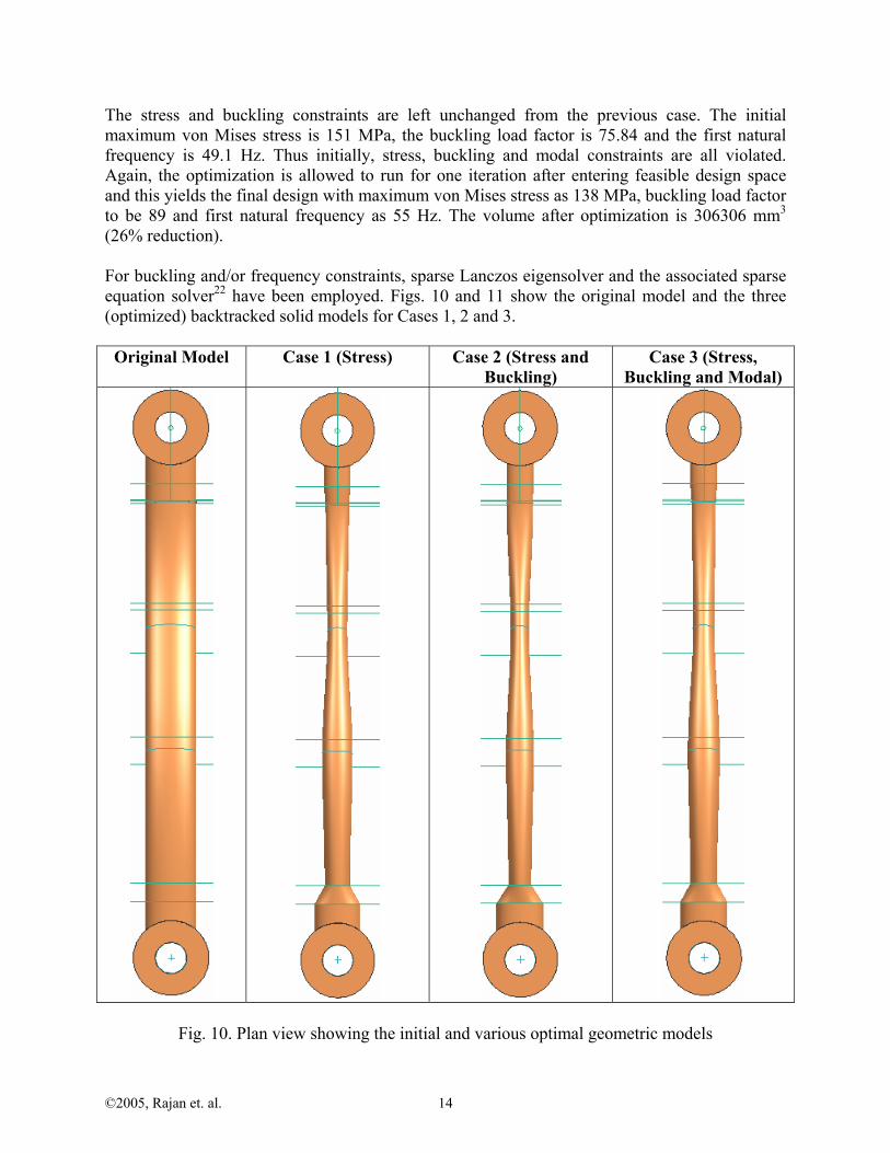
The stress and buckling constraints are left unchanged from the previous case. The initial maximum von Mises stress is 151 MPa, the buckling load factor is 75.84 and the first natural frequency is 49.1 Hz. Thus initially, stress, buckling and modal constraints are all violated. Again, the optimization is allowed to run for one iteration after entering feasible design space and this yields the final design with maximum von Mises stress as 138 MPa, buckling load factor to be 89 and first natural frequency as 55 Hz. The volume after optimization is 306306 mm3 (26% reduction). For buckling and/or frequency constraints, sparse Lanczos eigensolver and the associated sparse equation solver22 have been employed. Figs. 10 and 11 show the original model and the three (optimized) backtracked solid models for Cases 1, 2 and 3.

Original Model Case 1 (Stress) Case 2 (Stress and Buckling)

Case 3 (Stress, Buckling and Modal)

Fig. 10. Plan view showing the initial and various optimal geometric models

©2005, Rajan et. al. 15

Original Model Case 1 (Stress) Case 2 (Stress and Buckling)

Case 3 (Stress, Buckling and

Modal)

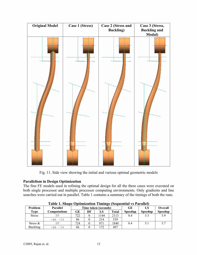
Fig. 11. Side view showing the initial and various optimal geometric models Parallelism in Design Optimization The fine FE models used in refining the optimal design for all the three cases were executed on both single processor and multiple processor computing environments. Only gradients and line searches were carried out in parallel. Table 1 contains a summary of the timings of both the runs.

Table 1. Shape Optimization Timings (Sequential vs Parallel) Time taken (seconds) Problem

Type Parallel

Computations GE DF LS Total GE

Speedup LS

Speedup Overall Speedup

SP 722 0 1144 2113 Stress -ge –ls 86 0 214 539

8.4 5.3 3.9

SP 724 0 871 1840 Stress & Buckling -ge –ls 86 0 172 497

8.4 5.1 3.7

©2005, Rajan et. al. 16

SP 721 0 1309 2274 Stress, Buckling & Modal

-ge –ls 86 0 214 538

8.4 6.11 4.2

As expected, parallelization of gradient calculations yields the best speedup especially since the number of design variables is a multiple of the number of available processors. In fact the speedup is better than expected linear speedup of 8.0. The direction-finding process hardly takes any time since the number of active constraints is small. The parallel line search yields decent speedup. It is not possible to obtain a linear speedup since all the processors cannot be kept equally busy during the three steps of the parallel LS algorithm. The overall speedup of 3.9 to 4.2 shows an overall efficiency of about 50% in the parallel computations.

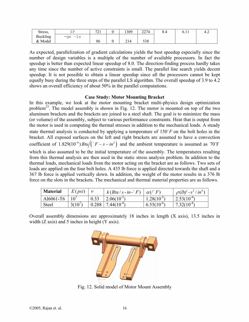
Case Study: Motor Mounting Bracket

In this example, we look at the motor mounting bracket multi-physics design optimization problem23. The model assembly is shown in Fig. 12. The motor is mounted on top of the two aluminum brackets and the brackets are joined to a steel shaft. The goal is to minimize the mass (or volume) of the assembly, subject to various performance constraints. Heat that is output from the motor is used in computing the thermal stresses in addition to the mechanical loads. A steady state thermal analysis is conducted by applying a temperature of 150 F on the bolt holes in the bracket. All exposed surfaces on the left and right brackets are assumed to have a convection coefficient of ( )6 21.829(10 ) Btu F s in− − − and the ambient temperature is assumed as 70 F which is also assumed to be the initial temperature of the assembly. The temperatures resulting from this thermal analysis are then used in the static stress analysis problem. In addition to the thermal loads, mechanical loads from the motor acting on the bracket are as follows. Two sets of loads are applied on the four bolt holes. A 435 lb force is applied directed towards the shaft and a 367 lb force is applied vertically down. In addition, the weight of the motor results in a 376 lb force on the slots in the brackets. The mechanical and thermal material properties are as follows.

Material ( )E psi ν ( / - - )k Btu s in F (/ )Fα 2 4( - / )lbf s inρAl6061-T6 107 0.33 2.06(10-3) 1.28(10-5) 2.53(10-4) Steel 3(107) 0.288 7.44(10-4) 6.55(10-6) 7.32(10-4)

Overall assembly dimensions are approximately 18 inches in length (X axis), 13.5 inches in width (Z axis) and 5 inches in height (Y axis).

Fig. 12. Solid model of Motor Mount Assembly

©2005, Rajan et. al. 17

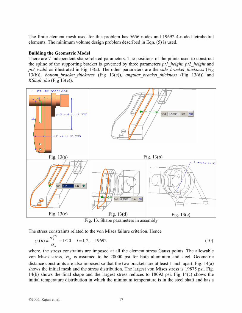
The finite element mesh used for this problem has 5656 nodes and 19692 4-noded tetrahedral elements. The minimum volume design problem described in Eqn. (5) is used. Building the Geometric Model There are 7 independent shape-related parameters. The positions of the points used to construct the spline of the supporting bracket is governed by three parameters pt1_height, pt2_height and pt2_width as illustrated in Fig 13(a). The other parameters are the side_bracket_thickness (Fig 13(b)), bottom_bracket_thickness (Fig 13(c)), angular_bracket_thickness (Fig 13(d)) and KShaft_dia (Fig 13(e)).

Fig. 13(a)

Fig. 13(b)

Fig. 13(c) Fig. 13(d)

Fig. 13(e) Fig. 13. Shape parameters in assembly

The stress constraints related to the von Mises failure criterion. Hence

( ) 1 0 1,2,...,19692VMi

ia

g iσσ

≡ − ≤ =x (10)

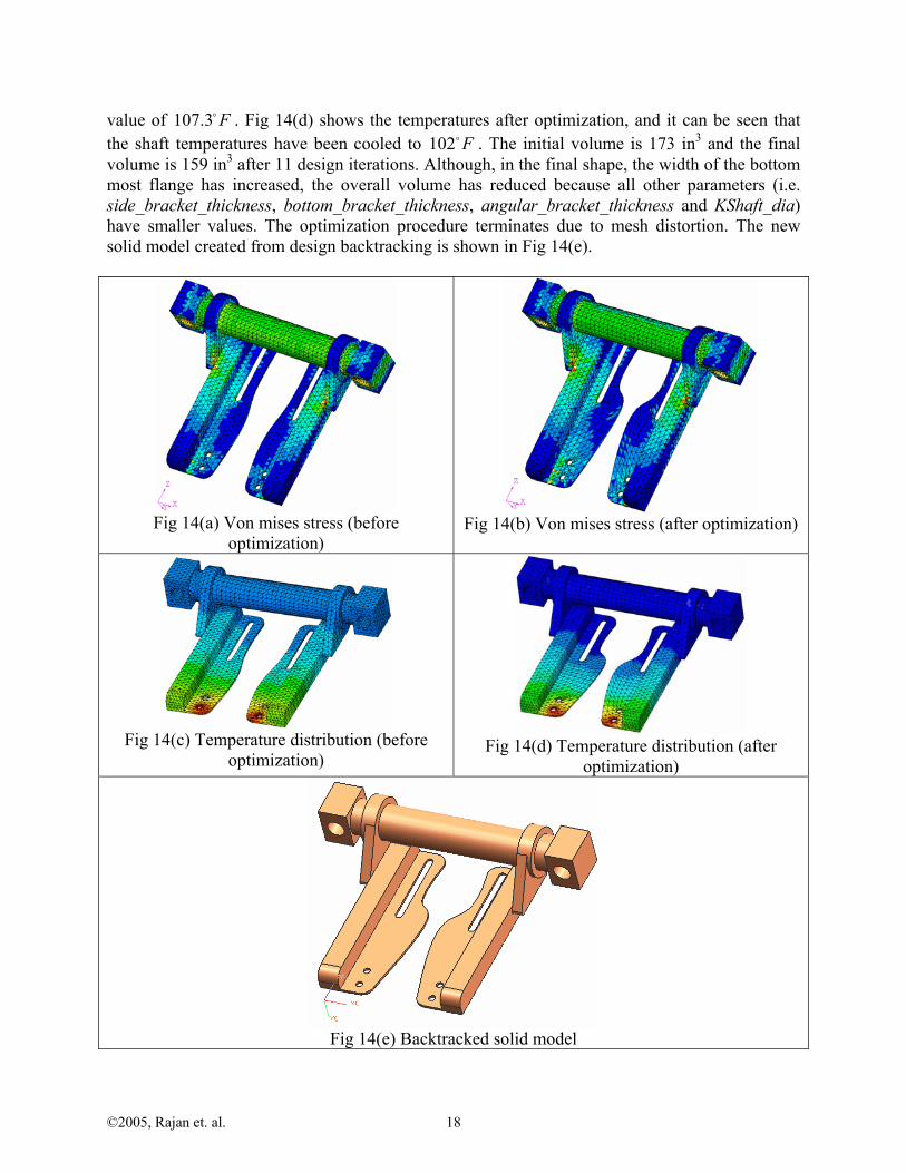
where, the stress constraints are imposed at all the element stress Gauss points. The allowable von Mises stress, aσ is assumed to be 20000 psi for both aluminum and steel. Geometric distance constraints are also imposed so that the two brackets are at least 1 inch apart. Fig. 14(a) shows the initial mesh and the stress distribution. The largest von Mises stress is 19875 psi. Fig. 14(b) shows the final shape and the largest stress reduces to 18092 psi. Fig 14(c) shows the initial temperature distribution in which the minimum temperature is in the steel shaft and has a

©2005, Rajan et. al. 18

value of 107.3 F . Fig 14(d) shows the temperatures after optimization, and it can be seen that the shaft temperatures have been cooled to 102 F . The initial volume is 173 in3 and the final volume is 159 in3 after 11 design iterations. Although, in the final shape, the width of the bottom most flange has increased, the overall volume has reduced because all other parameters (i.e. side_bracket_thickness, bottom_bracket_thickness, angular_bracket_thickness and KShaft_dia) have smaller values. The optimization procedure terminates due to mesh distortion. The new solid model created from design backtracking is shown in Fig 14(e).

Fig 14(a) Von mises stress (before

optimization)

Fig 14(b) Von mises stress (after optimization)

Fig 14(c) Temperature distribution (before

optimization)

Fig 14(d) Temperature distribution (after

optimization)

Fig 14(e) Backtracked solid model

©2005, Rajan et. al. 19

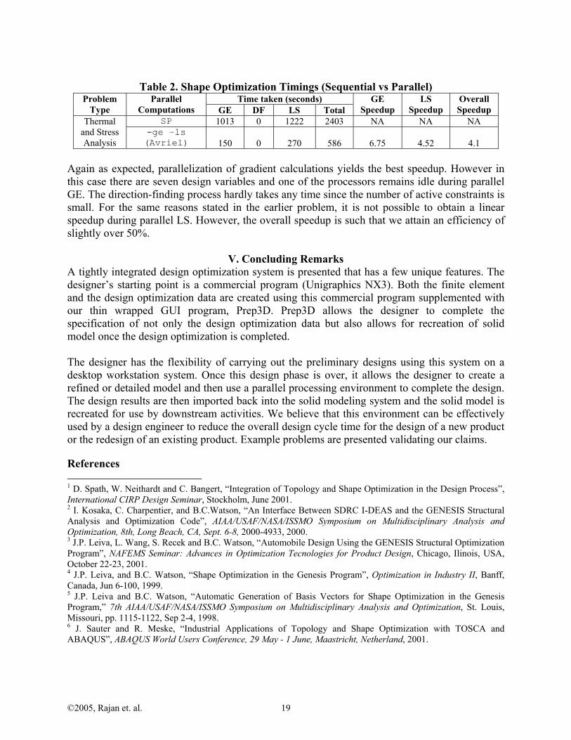
Table 2. Shape Optimization Timings (Sequential vs Parallel)

Time taken (seconds) Problem Type

Parallel Computations GE DF LS Total

GE Speedup

LS Speedup

Overall Speedup

SP 1013 0 1222 2403 NA NA NA Thermal and Stress Analysis

-ge –ls (Avriel) 150 0 270 586

6.75

4.52

4.1

Again as expected, parallelization of gradient calculations yields the best speedup. However in this case there are seven design variables and one of the processors remains idle during parallel GE. The direction-finding process hardly takes any time since the number of active constraints is small. For the same reasons stated in the earlier problem, it is not possible to obtain a linear speedup during parallel LS. However, the overall speedup is such that we attain an efficiency of slightly over 50%.

V. Concluding Remarks A tightly integrated design optimization system is presented that has a few unique features. The designer’s starting point is a commercial program (Unigraphics NX3). Both the finite element and the design optimization data are created using this commercial program supplemented with our thin wrapped GUI program, Prep3D. Prep3D allows the designer to complete the specification of not only the design optimization data but also allows for recreation of solid model once the design optimization is completed. The designer has the flexibility of carrying out the preliminary designs using this system on a desktop workstation system. Once this design phase is over, it allows the designer to create a refined or detailed model and then use a parallel processing environment to complete the design. The design results are then imported back into the solid modeling system and the solid model is recreated for use by downstream activities. We believe that this environment can be effectively used by a design engineer to reduce the overall design cycle time for the design of a new product or the redesign of an existing product. Example problems are presented validating our claims.

References 1 D. Spath, W. Neithardt and C. Bangert, “Integration of Topology and Shape Optimization in the Design Process”, International CIRP Design Seminar, Stockholm, June 2001. 2 I. Kosaka, C. Charpentier, and B.C.Watson, “An Interface Between SDRC I-DEAS and the GENESIS Structural Analysis and Optimization Code”, AIAA/USAF/NASA/ISSMO Symposium on Multidisciplinary Analysis and Optimization, 8th, Long Beach, CA, Sept. 6-8, 2000-4933, 2000. 3 J.P. Leiva, L. Wang, S. Recek and B.C. Watson, “Automobile Design Using the GENESIS Structural Optimization Program”, NAFEMS Seminar: Advances in Optimization Tecnologies for Product Design, Chicago, Ilinois, USA, October 22-23, 2001. 4 J.P. Leiva, and B.C. Watson, “Shape Optimization in the Genesis Program”, Optimization in Industry II, Banff, Canada, Jun 6-100, 1999. 5 J.P. Leiva and B.C. Watson, “Automatic Generation of Basis Vectors for Shape Optimization in the Genesis Program,” 7th AIAA/USAF/NASA/ISSMO Symposium on Multidisciplinary Analysis and Optimization, St. Louis, Missouri, pp. 1115-1122, Sep 2-4, 1998. 6 J. Sauter and R. Meske, “Industrial Applications of Topology and Shape Optimization with TOSCA and ABAQUS”, ABAQUS World Users Conference, 29 May - 1 June, Maastricht, Netherland, 2001.

©2005, Rajan et. al. 20

7 R. Meske, F. Mulfinger and O. Warmuth, “Topology and Shape Optimization of Components and Systems with Contact Boundary Conditions”, NAFEMS Seminar, Modeling of Assemblies and Joints for FE Analyses, 24-25. April, Wiesbaden, 2002. 8 B. Nima, A. Peter, F. Matthias, M. Fritz, S. Jürgen, M. Ottmar and P. Martin, “A New Approach for Sizing, Shape and Topology Optimization”, SAE International Congress and Exposition, Detroit, Michigan USA, February 26-29, 1996. 9 F. Dirschmid, “Optimization of Car Components using MSC/CONSTRUCT”, FE-DESIGN MSC's 1st Worldwide Automotive Conference, Munich, 1999. 10 http://www.ansys.com/products/workbench-simulation.asp. 11 http://www.ansys.com/products/geometry-interfaces.asp. 12 http://www.ugs.com/products/nx/simulation/prod_apps/opt_wizard.shtml. 13 http://www.altair.com/software/hw_os.htm. 14 S.D. Rajan, S-W.Chin and L.Gani, "Towards a Practical Design Optimization Tool", Microcomputers in Civil Engineering, 11, 259-274, 1996. 15 A.D. Belegundu and S.D. Rajan, “A Shape Optimization Approach Based on Natural Design Variables and Shape Functions", Computer Methods in Applied Mechanics and Engineering, 66, 87-106, 1988. 16 Belegundu, A.D., Damle, A., Rajan, S.D., Dattaguru, B. and St. Ville, J., “Parallel Line Search in Method of Feasible Directions”, Optimization and Engineering Journal, Optimization and Engineering Journal, 5, 2004, pp. 379-288. 17 Nguyen, D.T., “Nonlinear constrained optimization and parallel processing for golden block line search”, Computer Assisted Mechanics and Engineering Sciences, Vol. 6, No. 3, 8th International Conference on Numerical Mathematics and Computational Mechanics (NMCM98), Miskolc, Hungary, 1998, pp. 469-477. 18 Rajan, S.D., Belegundu, A.D., Damle, A.S., Lim, H. and St. Ville, J., “General Implementation of Multilevel Parallelization in a Gradient-based Design Optimization Algorithm”, submitted to AIAA Journal, 2005. 19 A.D. Belegundu, A. Damle, D. Lau and S.D. Rajan, “Coarse and Fine-Grain Nested Parallelism for Finite-Element Based Design Optimization”, submitted to Optimization and Engineering Journal, 2005. 20 Hawthorne & York, Intl, HYI-3D Design Optimization System, Phoenix, AZ, 2005. 21 N.H Kim, K.K. Choi and M.E. Botkin, “Numerical Method for Shape Optimization using Meshfree Method”, Structural Multidisciplinary Optimization, 24-6, 418-429, 2003. 22 D.T. Nguyen, Finite Element Methods: Parallel-Sparse Statics and Eigensolutions, Springer, expected Feb. 2006. 23 Algor Tutorial, Pittsburgh, PA, 2004.