1

Multiobjective Flexible Job Shop Scheduling with Overlapping in Operations

Mehrzad Abdi Khalife a∗, Babak Abbasi b, Esmaeil Mehdizadeh a,

Amir Hossein Kamali Dolat Abadia

a Faculty of Industrial and Mechanical Engineering, Qazvin Islamic Azad University, Qazvin, Iran b

Department of Industrial Engineering, Sharif University of Technology, Tehran, Iran

Abstract

This paper considers a multiobjective approach on flexible job shop scheduling problem

with overlapping in operations assumption. The makespan, the total machine work loading

time as well as the critical machine work loading time are taken into account as objective

functions in a multiobjective mixed integer linear model. The branch and bound (B&B)

method is employed to solve the small size problems, while variable neighborhood search

(VNS) and simulated annealing (SA) algorithms are developed for assignment and scheduling

phases for large scale ones then select proper combination of SA and VNS algorithms with

TOPSIS method. The proposed algorithm parameters are tuned with Taguchi experimental

design method. The performance analysis of proposed method is investigated due to its

accuracy and agility. .

Keywords

Flexible Job Shop Scheduling; FJSP with Overlapping; Multi-objective optimization; Variable Neighborhood Search; Simulated Annealing; Combinatorial optimization; TOPSIS.

1. Introduction

The Flexible Job Shop Problem (FJSP) is an extension of the classical JSP which allows an operation to

be processed by any machine from a given set. The problem is to assign each operation to a machine and

to order the operations on the machines, such that the maximal completion time (makespan) of all

operations is minimized.

∗ Corresponding author: Address: First Floor, No.15, Helalli St., South Daneshgah St., Jamhory St., Tehran, Iarn; Post Code: 1316775566; Tel:+989358064224; Fax:+982188929120 E-mail addresses: mehrzadabdi@gmail.com (M.Abdi), Abbasi@Sharif.edu (B. Abbasi),emehdi@qiau.ac.ir (E. Mehdizahe), amir_kamaly2002@yahoo.com (A.Kamaly)

2

The job shop scheduling problems as a NP-hard problem firstly introduced by Garey et.al (1976) [1].

There is an extensive literature in JSP for instances see Gen and Cheng (1997) [2], Gen and Cheng (2000)

[3] and Blazewicz et.al (1996) [4]. The literature of FJSP is considerably sparser than the literature of

JSP. Bruker and Schlie (1990) [5] were amongst the first researchers to address this problem. They

developed a polynomial algorithm for solving the flexible job-shop problem with two jobs. In general

situations many researchers used heuristics and meta-heuristic algorithms to approach FJSP.

Two types of approaches have been used in solving a FJSP which are hierarchical approach and

integrated approach. In the former approach assignment of operations to machines and the sequencing of

operations on the resources or machines are treated separately, i.e. assignment and sequencing are

considered independently, whereas in integrated approach, assignment and sequencing are consolidated.

The idea behind the Hierarchical approach is decomposing the problem in order to reduce its complexity.

This type of approach is natural for FJSP since the routing and the scheduling sub-problems can be

separated [6]. Brandimarte (1993) [7] was the first one who used decomposition approach for the FJSP.

He solved the routing sub-problem by using dispatching rules and then focused on the scheduling sub-

problem, which is solved using a tabu search algorithm. Li, and Nagi (1999) developed a similar approach

for scheduling a flexible manufacturing system [8].

Integrated approach attends assignment and scheduling at the same time. Hurink et.al (1994) proposed a

tabu search algorithm in which reassignment and rescheduling are considered as two different types of

moves [9]. Dauzere-peres (1997) defined a neighborhood structure for the problem where there is no

distinction between reassigning and re-sequencing an operation then, the Tabu Search (TS) procedure was

proposed [10]. Mastrolill and Gambardella (2002) improved Dauzere-Peres’ tabu search techniques and

presented two neighborhood functions [11]. Rigoa (2004) used TS in tardiness minimization in a FJSP

[12].

Kacem et.al (2002) [13], Zandieh et.al (2008) [14] and Gao et.al (2008) [15] as well as Pezzella et.al

(2008) [16] applied Genetic Algorithm (GA) and Xia and Wu (2005) used Prato Swam Optimization

(PSO) algorithm for solving FJSP.

Alvarez-Valdes et.al (2005) [17] augmented an overlapping assumption in operations in FJSP and

presented a heuristic method to solve it. In overlapping, the operations to be performing on the jobs can

overlap. They provided an application in glass industry. Fattahi et.al (2008) [18] used SA in FJSS with

overlapping assumption in order to minimize maximal completion time.

In multiobjective view in the FJSP, Kacem et.al (2002) considered minimizing the overall completion

time (makespan) and the total workload of the machines simultaneously in the FJSP. Xia and Wu (2005)

considered three objectives that were the makespan (maximal completion time), the total workload of

machines, and the workload of the critical machine. They used a PSO to assign operations on machines

3

and SA algorithm to schedule operations on each machine. Gao et.al (2008) applied a hybrid genetic and

variable neighborhood descent algorithm for the multiobjective FJSP. The objective functions were

minimizing makespan, minimizing maximal machine workload and minimizing total workload. Zhang

et.al (2008) [19] used three objectives same Xia and Wu (2005) and used PSO to assign operations on

machines and to schedule operations on each machine, and TS was applied to local search for the

scheduling sub-problem originating from each obtained solution. Recently Xing et.al (2009) presented a

simulation model in FJSS and used makespan, total machine work loading time and critical machine work

loading time as objective functions [20].

In this article, we applied multiobjective approach for FJSP with overlapping in operations and used the

objectives addressed in Xia and Wu (2005), Zhang et.al (2008) and Xing et.al (2009). A mixed integer

linear model is presented and we use the branch and bound (B&B) algorithm to solve it. For large sale

problems, a hybrid VNS and SA algorithm is developed. The proposed algorithm parameters are tuned in

experimental design and analysis procedure.

The paper is organized as following manner: in the next section, mathematical model of the problem is

presented. Section 3 introduces VNS and SA algorithms briefly and describes these algorithms and our

proposed method to solve FJSSP. The Section 4 explains how to set algorithm parameters. The Sections 5

consider numerical examples and discussion on obtain results. Section 6 contains conclusion and future

lines for research.

2. Problem description and formulation

Problem consists a set of machines denotes by M, = { , , … , } and n jobs. The set of sequence

operation make a job shown by , ; that i is the job number and represents number of operations

required for a particular job i.

The assumptions in the problem are:

• Operation time is dependent on selected machine.

• There is no priority for operations.

• Setup time is independent of sequencing and included in operation time.

• There is no need to rework.

• All operations are available in the start time.

• Each machine can work on one operation in each time.

• There is no space capacity restriction before and after a machine

• All machines are available.

4

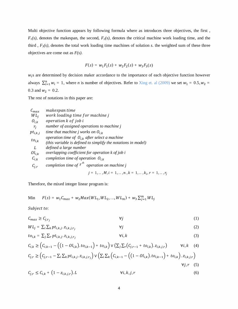
Multi objective function appears by following formula where as introduces three objectives, the first ,

F1(s), denotes the makespan, the second, F2(s), denotes the critical machine work loading time, and the

third , F3(s), denotes the total work loading time machines of solution s. the weighted sum of these three

objectives are come out as F(s).

( ) = ( ) + ( ) + ( ) s are determined by decision maker accordance to the importance of each objective function however

always ∑ = 1 , where n is number of objectives. Refer to Xing et. al (2009) we set = 0.5, =0.3 and = 0.2.

The rest of notations in this paper are:

ℎ , number of assigned operations to machine j , , time that machine j works on , , operation time of , after select a machine (this variable is defined to simplify the notations in model) defined a large number , overlapping coefficient for operation k of job i , completion time of operation , , completion time of

thr operation on machine j

= 1, … , , = 1, … , , = 1, … , , = 1, … , Therefore, the mixed integer linear program is:

Min ( ) = + ( , , … , ) + ∑ : ≥ , ∀ (1) = ∑ ∑ , , . , , , ∀ (2) , = ∑ ∑ , , . , , , ∀ , (3) , ≥ , − 1 − , . , + , ∨ ∑ ∑ , + , . , , , ∀ , (4) , ≥ , −∑ ∑ , , . , , , ∨ ∑ ∑ , − 1 − , . , + , . , , ,

∀ , (5) , ≤ , + 1 − , , , . ∀ , , , (6)

5

, ≤ , + 1 − , , , . ∀ , , , (7) ∑ , , , = 1 ∀ , (8) ∑ , , , = 1 ∀ (9)

, , , = 1 , ℎ 0 ℎ

The constraint (1) defines first objective i.e. the makespan. The constraint (2) defines each machine work

loading time, and is used to define second and third objectives. The constraint (3) calculates the operation

time of , after assigning it to a machine, this constraint is added to define , and simplifying

following constraints.

Overlapping assumption allows before completion of , next operation of job , , be started on an

idle machine that can work on , . In this purpose , indicates that , can be started on a

possible idle machine after passing , , . , time from start time of , .

The constraints (4) and (5) calculate completion time of operation on machine j. The first part in

constraint (4) is considering overlapping permission and calculating possible start time of operation , .

The second part of constraint (4) calculates the completion time of other assigned operations in machine j

before operation , and forces each machine to process one operation at a time. For ensure each

operation , is started when it is assigned to a idle machine constraints (6) and (7) are written.

Operation , may be started after completion of , or may be started before completion of , and

after , , . , , the constraint (5) contrasts these situations. The constraints (6) and (7) oblige all

operations assigned properly in defined sequence. Result of assignment and sequence of operations save

in , , , .

3- SA and VNS algorithms

In this part we glance on a SA and VNS algorithms which are used in our proposed method.

3-1 VNS algorithm

VNS algorithm is a systematic search algorithm which strives to find an optimal solution or an acceptable

and near optimum solution, and it becomes a powerful algorithm in computation [21]. The main idea of

VNS is very simple; with dislocated neighborhoods and local search in these neighborhoods try to

6

improvement solutions [22]. This algorithm design for search in set of N , k = 1 , … , k with

predefined structure. Search start after defining the initial solution. The general steps of VNS are:

1- Select a stopping criterion, (usually maximal allowed CPU time and repeat the step 3-4) 2- Repeat following steps: 2-1-Shaking

Generate a point, y, randomly from the th neighborhood of ( )( )kx y N x∈ 2-2- Local search

Apply local search methods when y is the initial solution to obtain a local optimum given by y ′ .

3- Neighborhood change If this local optimum is better than the current solution (at the beginning of algorithm it is initial solution), replace obtained local optimum as best solution hitherto ( y x′ → ) ,and continue till k=kmax

4- 1k k+ → 5- Stop if stop condition is met.

3-2 SA algorithm

A simulated annulling algorithm is a suitable search tools that inspiration from physical annealing

process and statistic methods [23]. Pincus in 1970 proof that this algorithm is capable to minimizing

mathematical function [24]. SA algorithm with generating different neighborhoods tries to convergent to

optimum objective function. For escape from local optimum in this algorithm accept bad solution. In each

iteration existing solution is shown by , and its objective function is shown by ( ), neighborhood is

from set ( ) that define by ′ and it objective function is ( ′).

In each iteration computed ∆= ( ) − ( ) and if objective function is maximization when ∆≥ 0 ′ its

substitute by x and otherwise with probability P = e( ∆/ ) accept x′ solution. For survey acceptance

worth solution generate a random number R~uni(0,1) and if term < is met solution ′ accept.

Acceptance probability for worth solutions effective factors are Δ, and ; whatever Δ is small the

probability of acceptance worth solution increase, and also if is higher the probability of acceptance

increase too. Temperature is control by cooling schema that it decreases initial temperature; cooling

schema is very important for finding good solution. Available cooling schemas theoretically are try

convergence to optimum solution, but in practical used simplify method for cooling schema.

Generally for reduce temperature in SA algorithm use steps, these steps start with initial temperature and by use coefficient , (0 < < 1) reduce. Initial temperature should enough high that the

algorithm in first iteration can accept worth solution with 80 percent probability. In each step of in SA

algorithm it generate some neighborhoods and evaluate them with current temperature = ∗ .

Generally call this cooling schema, cooling chain or Markov chain.

7

4- Proposed algorithm

In this section our developed algorithm based on above meta heuristic algorithms is described.

4-1- Solution decoding

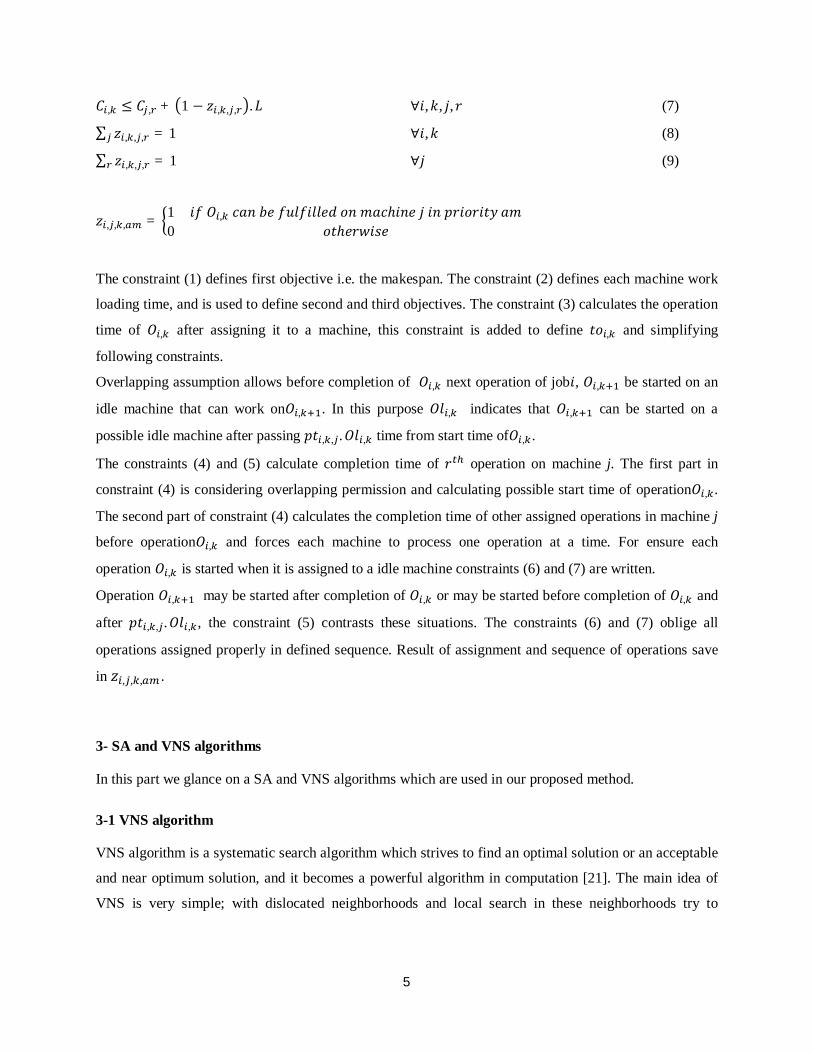
Solution is decoded in two vectors. First vector define assigned machine to operation, and second one

define sequence of the operation on machine. For example in Fig (1) position 6 indicates is assigned

to the first machine on the second sequence.

Fig. 1: solution decoding

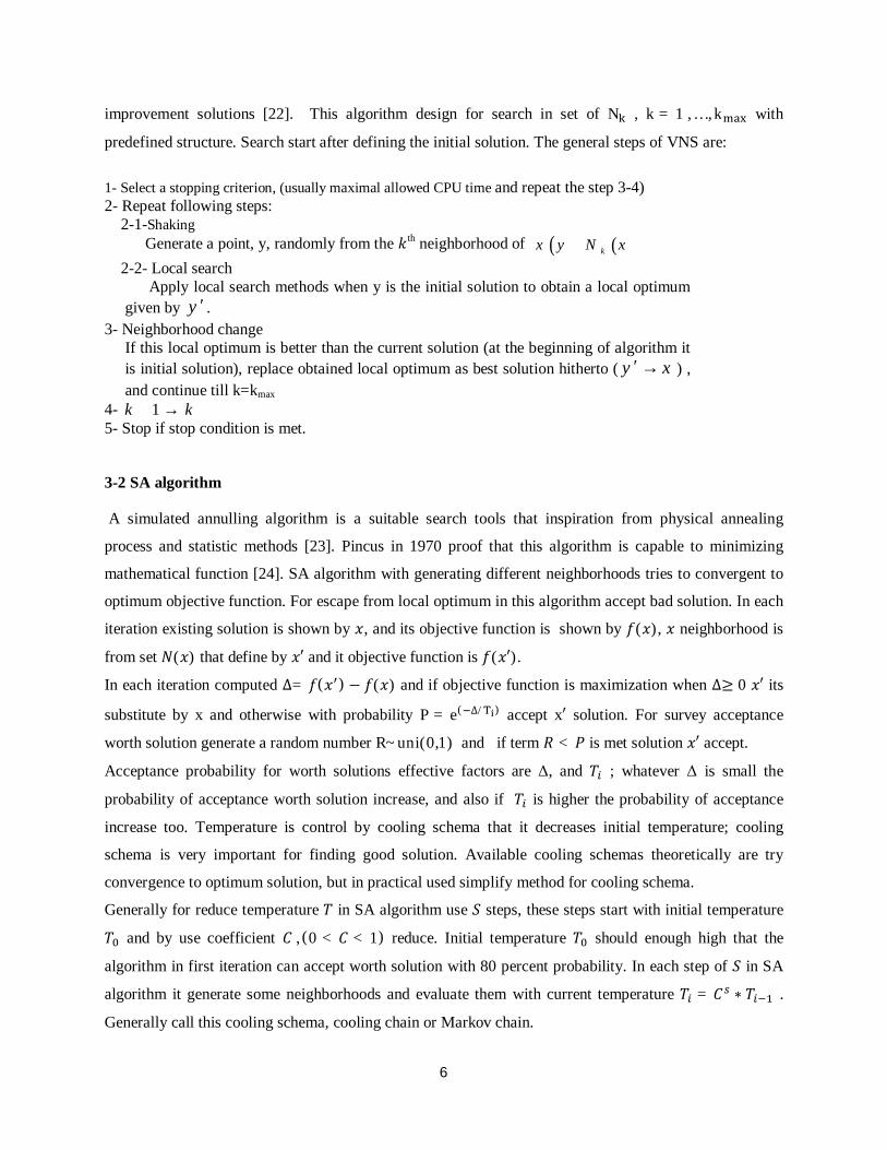
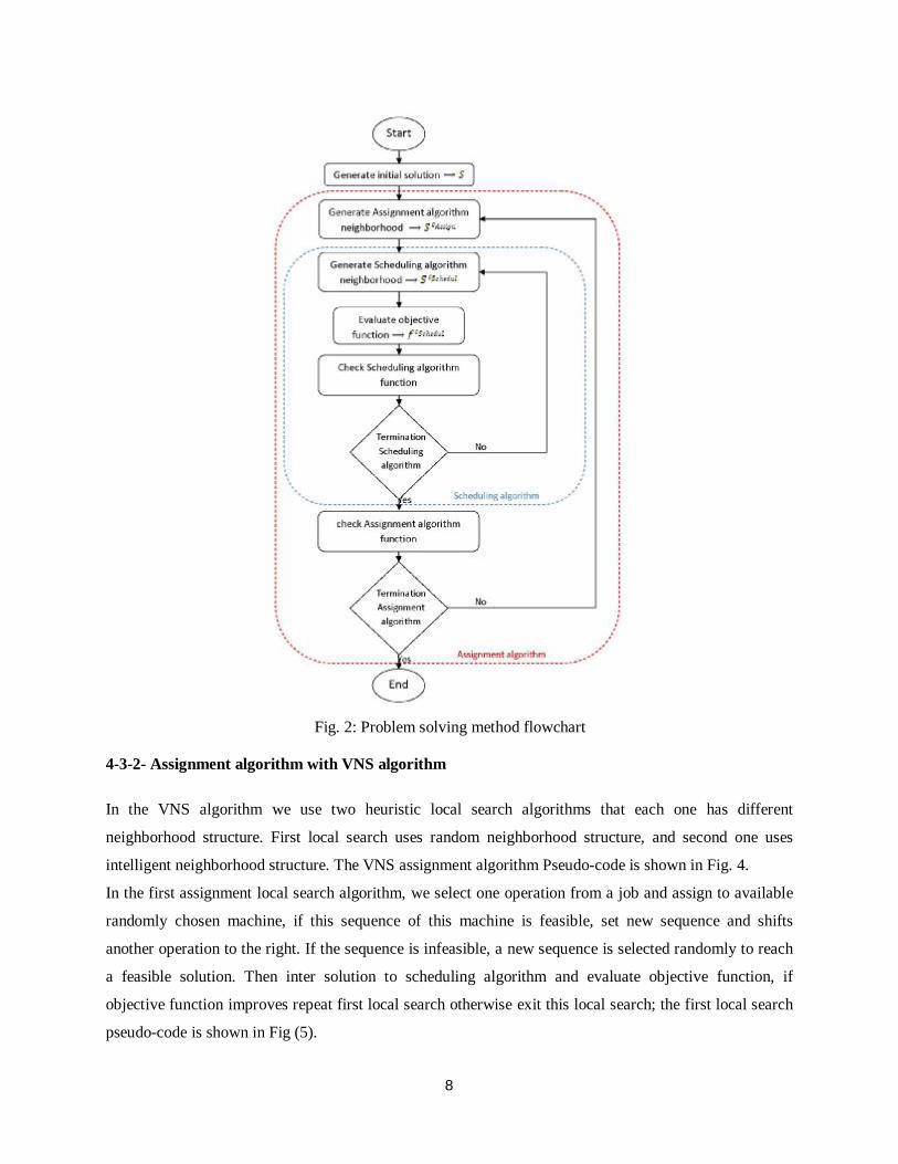
4-2- Solving method

For solving problem we pursue decomposition approach. We use a separate algorithm for each stage, i.e

assignment and scheduling. A flow chart to depict the proposed method is shown is Fig (2). We use apply

both VNS and SA algorithms in assignment and scheduling phases. Hence, we have four alternatives. All

these combinations are evaluated and compared together.

4-3- Assignment algorithms

In this part we apply SA and VNS algorithms in assignment stage.

4-3-1 Assignment algorithm with SA algorithm

We apply the SA algorithm described in section 2 in assignment phase. Fig (3) shows SA assignment

algorithm pseudo-code. In this algorithm is initial temperature, define final temperature, define

algorithm temperature in ith iteration of algorithm, is maximum allowed iteration, and is number

of iteration in each temperature. In order to generate neighborhood, we choose an operation randomly and

then select another machine which is not assigned yet randomly and substitute them. This machine

sequence is preserved and next operation shift to the right. If the sequence scheduling is not feasible, we

generate a random sequence to catch a feasible solution.

1 3 4 5 2 1 3 2 4 2 1 1 2 2 1 1 2 1 2 1 3 3

Operation is operating on machine 1 in the second sequence

8

Fig. 2: Problem solving method flowchart

4-3-2- Assignment algorithm with VNS algorithm

In the VNS algorithm we use two heuristic local search algorithms that each one has different

neighborhood structure. First local search uses random neighborhood structure, and second one uses

intelligent neighborhood structure. The VNS assignment algorithm Pseudo-code is shown in Fig. 4.

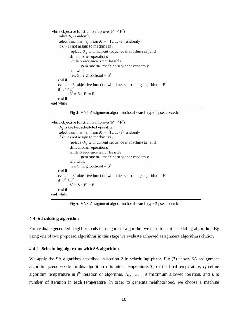
In the first assignment local search algorithm, we select one operation from a job and assign to available

randomly chosen machine, if this sequence of this machine is feasible, set new sequence and shifts

another operation to the right. If the sequence is infeasible, a new sequence is selected randomly to reach

a feasible solution. Then inter solution to scheduling algorithm and evaluate objective function, if

objective function improves repeat first local search otherwise exit this local search; the first local search

pseudo-code is shown in Fig (5).

9

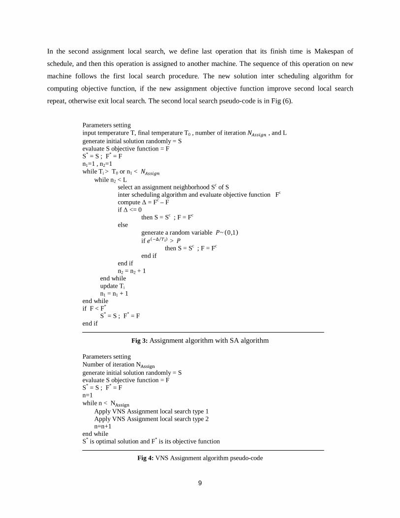
In the second assignment local search, we define last operation that its finish time is Makespan of

schedule, and then this operation is assigned to another machine. The sequence of this operation on new

machine follows the first local search procedure. The new solution inter scheduling algorithm for

computing objective function, if the new assignment objective function improve second local search

repeat, otherwise exit local search. The second local search pseudo-code is in Fig (6).

Parameters setting input temperature T, final temperature T0 , number of iteration , and L generate initial solution randomly = S evaluate S objective function = F S* = S ; F* = F n1=1 , n2=1 while Ti > T0 or n1 < while n2 < L select an assignment neighborhood Sc of S inter scheduling algorithm and evaluate objective function Fc compute Δ = Fc – F if Δ <= 0 then S = Sc ; F = Fc else generate a random variable ~(0,1) if ( ⁄ ) > then S = Sc ; F = Fc end if end if n2 = n2 + 1 end while update Ti n1 = n1 + 1 end while if F < F* S* = S ; F* = F end if

Fig 3: Assignment algorithm with SA algorithm

Parameters setting Number of iteration N generate initial solution randomly = S evaluate S objective function = F S* = S ; F* = F n=1 while n < N Apply VNS Assignment local search type 1 Apply VNS Assignment local search type 2 n=n+1 end while S* is optimal solution and F* is its objective function

Fig 4: VNS Assignment algorithm pseudo-code

10

while objective function is improve (Fc < F*) select randomly select machine from = {1, … , } randomly if is not assign to machine replace with current sequence in machine and shift another operations while S sequence is not feasible generate machine sequence randomly end while new S neighborhood = Sc end if evaluate Sc objective function with inter scheduling algorithm = Fc if Fc < F* S* = S ; F* = F end if end while

Fig 5: VNS Assignment algorithm local search type 1 pseudo-code

while objective function is improve (Fc < F*) is the last scheduled operation select machine from = {1, … , } randomly if is not assign to machine replace with current sequence in machine and shift another operations while S sequence is not feasible generate machine sequence randomly end while new S neighborhood = Sc end if evaluate Sc objective function with inter scheduling algorithm = Fc if Fc < F* S* = S ; F* = F end if end while

Fig 6: VNS Assignment algorithm local search type 2 pseudo-code

4-4- Scheduling algorithm

For evaluate generated neighborhoods in assignment algorithm we need to start scheduling algorithm. By

using one of two proposed algorithms in this stage we evaluate achieved assignment algorithm solution.

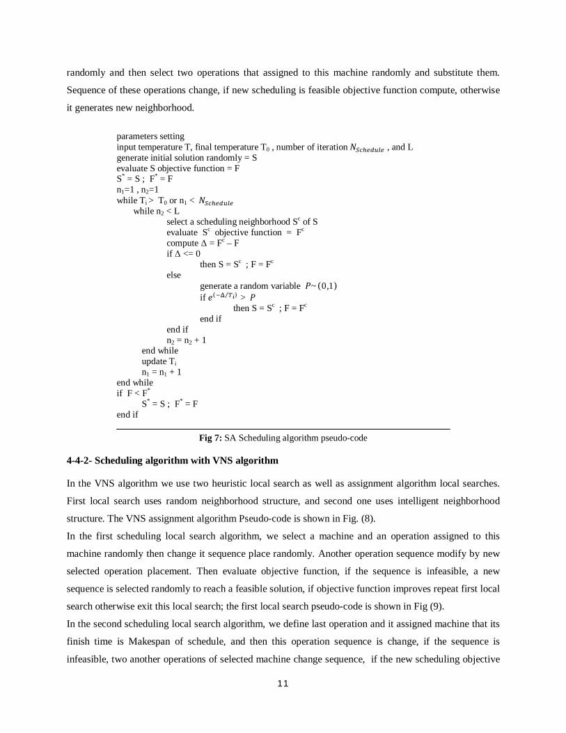
4-4-1- Scheduling algorithm with SA algorithm

We apply the SA algorithm described in section 2 in scheduling phase. Fig (7) shows SA assignment

algorithm pseudo-code. In this algorithm is initial temperature, define final temperature, define

algorithm temperature in ith iteration of algorithm, is maximum allowed iteration, and is

number of iteration in each temperature. In order to generate neighborhood, we choose a machine

11

randomly and then select two operations that assigned to this machine randomly and substitute them.

Sequence of these operations change, if new scheduling is feasible objective function compute, otherwise

it generates new neighborhood.

parameters setting input temperature T, final temperature T0 , number of iteration , and L generate initial solution randomly = S evaluate S objective function = F S* = S ; F* = F n1=1 , n2=1 while Ti > T0 or n1 < while n2 < L select a scheduling neighborhood Sc of S evaluate Sc objective function = Fc compute Δ = Fc – F if Δ <= 0 then S = Sc ; F = Fc else generate a random variable ~(0,1) if ( ⁄ ) > then S = Sc ; F = Fc end if end if n2 = n2 + 1 end while update Ti n1 = n1 + 1 end while if F < F* S* = S ; F* = F end if

Fig 7: SA Scheduling algorithm pseudo-code

4-4-2- Scheduling algorithm with VNS algorithm

In the VNS algorithm we use two heuristic local search as well as assignment algorithm local searches.

First local search uses random neighborhood structure, and second one uses intelligent neighborhood

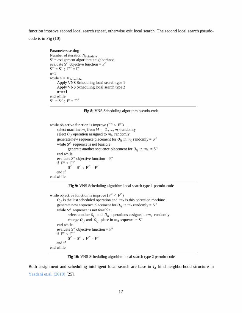
structure. The VNS assignment algorithm Pseudo-code is shown in Fig. (8).

In the first scheduling local search algorithm, we select a machine and an operation assigned to this

machine randomly then change it sequence place randomly. Another operation sequence modify by new

selected operation placement. Then evaluate objective function, if the sequence is infeasible, a new

sequence is selected randomly to reach a feasible solution, if objective function improves repeat first local

search otherwise exit this local search; the first local search pseudo-code is shown in Fig (9).

In the second scheduling local search algorithm, we define last operation and it assigned machine that its

finish time is Makespan of schedule, and then this operation sequence is change, if the sequence is

infeasible, two another operations of selected machine change sequence, if the new scheduling objective

12

function improve second local search repeat, otherwise exit local search. The second local search pseudo-

code is in Fig (10).

Parameters setting Number of iteration N Sc = assignment algorithm neighborhood evaluate Sc objective function = Fc Sc* = Sc ; Fc* = Fc n=1 while n < N Apply VNS Scheduling local search type 1 Apply VNS Scheduling local search type 2 n=n+1 end while Sc = Sc* ; Fc = Fc*

Fig 8: VNS Scheduling algorithm pseudo-code

while objective function is improve (F'c < Fc*) select machine from = {1, … , } randomly select operation assigned to randomly generate new sequence placement for in randomly = S'c while S'c sequence is not feasible generate another sequence placement for in = S'c end while evaluate S'c objective function = F'c if F'c < Fc* Sc* = S'c ; Fc* = F'c end if end while

Fig 9: VNS Scheduling algorithm local search type 1 pseudo-code

while objective function is improve (F'c < Fc*) is the last scheduled operation and is this operation machine generate new sequence placement for in randomly = S'c while S'c sequence is not feasible select another and ́ ́ operations assigned to randomly change and ́ ́ place in sequence = S'c end while evaluate S'c objective function = F'c if F'c < Fc* Sc* = S'c ; Fc* = F'c end if end while

Fig 10: VNS Scheduling algorithm local search type 2 pseudo-code Both assignment and scheduling intelligent local search are base in kind neighborhood structure in

Yazdani et.al. (2010) [25].

13

5- Algorithm setting

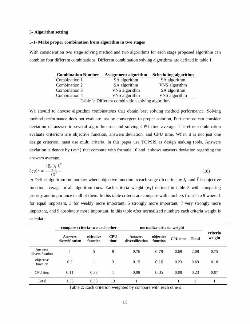
5-1- Make proper combination from algorithm in two stages

With consideration two stage solving method and two algorithms for each stage proposed algorithm can

combine four different combinations. Different combination solving algorithms are defined in table 1.

Scheduling algorithm Assignment algorithm Combination Number

SA algorithm SA algorithm Combination 1 algorithm VNS SA algorithm Combination 2

SA algorithm algorithm VNS Combination 3 algorithm VNS algorithm VNS Combination 4

Table 1: Different combination solving algorithm

We should to choose algorithm combinations that obtain best solving method performance. Solving

method performance does not evaluate just by convergent to proper solution, Furthermore can consider

deviation of answer in several algorithm run and solving CPU time average. Therefore combination

evaluate criterions are objective function, answers deviation, and CPU time. When it is not just one

design criterion, must use multi criteria. In this paper use TOPSIS as design making tools. Answers

deviation is denote by ( ) that compute with formula 10 and it shows answers deviation regarding the

answers average.

( ) = ∑ ̅ ̅ (10)

Define algorithm run number where objective function in each stage th define by , and ̅ is objective

function average in all algorithm runs. Each criteria weight ( ) defined in table 2 with comparing

priority and importance in all of them. In this table criteria are compare with numbers from 1 to 9 where 1

for equal important, 3 for weakly more important, 5 strongly more important, 7 very strongly more

important, and 9 absolutely more important. In this table after normalized numbers each criteria weight is

calculate.

compare criteria two each other normalize criteria weight criteria weight Answers

diversification objective function

CPU time

Answers diversification

objective function CPU time Total

Answers diversification 1 5 9 0.76 0.79 0.69 2.08 0.75

objective function 0.2 1 3 0.15 0.16 0.23 0.69 0.18

CPU time 0.11 0.33 1 0.08 0.05 0.08 0.23 0.07

Total 1.33 6.33 13 1 1 1 3 1 Table 2: Each criterion weighted by compare with each others

14

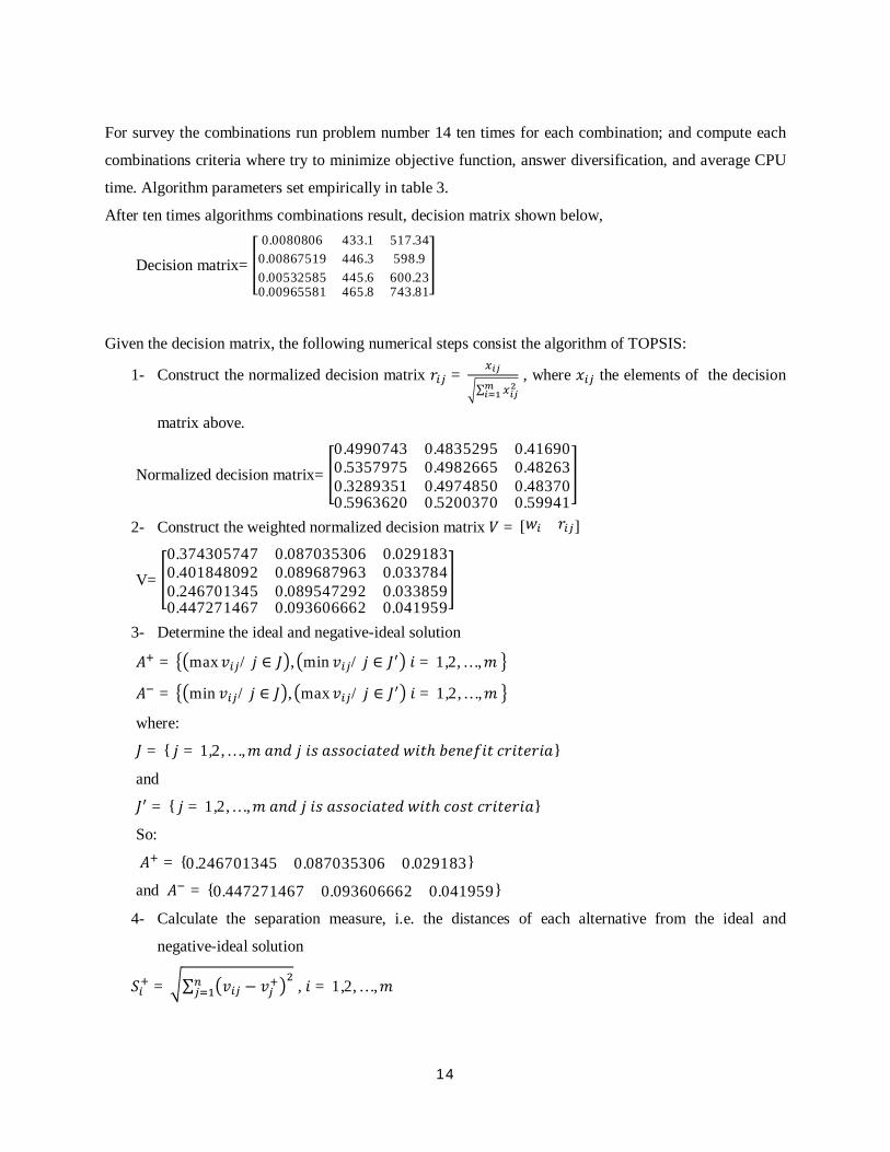
For survey the combinations run problem number 14 ten times for each combination; and compute each

combinations criteria where try to minimize objective function, answer diversification, and average CPU

time. Algorithm parameters set empirically in table 3.

After ten times algorithms combinations result, decision matrix shown below,

Decision matrix= 0.0080806 433.1 517.340.00867519 446.3 598.90.00532585 445.6 600.230.00965581 465.8 743.81

Given the decision matrix, the following numerical steps consist the algorithm of TOPSIS:

1- Construct the normalized decision matrix = ∑ , where the elements of the decision

matrix above.

Normalized decision matrix= 0.4990743 0.4835295 0.416900.5357975 0.4982665 0.482630.3289351 0.4974850 0.483700.5963620 0.5200370 0.59941 2- Construct the weighted normalized decision matrix = [ ]

V= 0.374305747 0.087035306 0.0291830.401848092 0.089687963 0.0337840.246701345 0.089547292 0.0338590.447271467 0.093606662 0.041959 3- Determine the ideal and negative-ideal solution = max / ∈ , min / ∈ = 1,2, … , = min / ∈ , max / ∈ = 1,2, … , where: = { = 1,2, … , ℎ }

and = { = 1,2, … , ℎ }

So:

= {0.246701345 0.087035306 0.029183}

and = {0.447271467 0.093606662 0.041959}

4- Calculate the separation measure, i.e. the distances of each alternative from the ideal and

negative-ideal solution = ∑ − , = 1,2, … ,

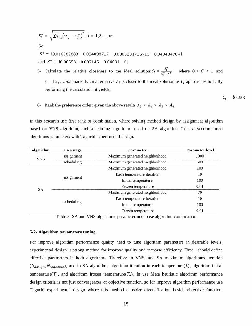
15

= ∑ − , = 1,2, … , So:

= {0.016282883 0.024098717 0.0000281736715 0.040434764}

and = {0.00553 0.002145 0.04031 0}

5- Calculate the relative closeness to the ideal solution: = , where 0 < < 1 and = 1,2, … , apparently an alternative is closer to the ideal solution as approaches to 1. By

performing the calculation, it yields: = {0.2535336- Rank the preference order: given the above results > > >

In this research use first rank of combination, where solving method design by assignment algorithm

based on VNS algorithm, and scheduling algorithm based on SA algorithm. In next section tuned

algorithms parameters with Taguchi experimental design.

algorithm Uses stage parameter Parameter level

VNS assignment Maximum generated neighborhood 1000 scheduling Maximum generated neighborhood 500

SA

assignment

Maximum generated neighborhood 100 Each temperature iteration 10

Initial temperature 100 Frozen temperature 0.01

scheduling

Maximum generated neighborhood 70 Each temperature iteration 10

Initial temperature 100 Frozen temperature 0.01

Table 3: SA and VNS algorithms parameter in choose algorithm combination

5-2- Algorithm parameters tuning

For improve algorithm performance quality need to tune algorithm parameters in desirable levels,

experimental design is strong method for improve quality and increase efficiency. First should define

effective parameters in both algorithms. Therefore in VNS, and SA maximum algorithms iteration

( , ), and in SA algorithm; algorithm iteration in each temperature( ), algorithm initial

temperature( ), and algorithm frozen temperature( ). In use Meta heuristic algorithm performance

design criteria is not just convergences of objective function, so for improve algorithm performance use

Taguchi experimental design where this method consider diversification beside objective function.

16

Genichi Taguchi in 1960's present experimental design with orthogonal arrays that control effective factor

with interior orthogonal array and noise factors (uncontrollable factors) with exterior orthogonal array.

For control the quality factors experiment compute signal-to-noise (S/N) ration from response variable. In

Taguchi definition regarding to S/N ration results of experimental designed, quality has minimum

diversification and improve algorithm performance use mean response variable for best algorithm

performance.

Generally parameters experimental method can describe as follow:

1- Calculate effective factors S/N ration and mean response variables, then experimental design S/N

ratio and mean response are test.

2- For each factor, define that one's has significant impact on S/N ratio, then select maximum S/N

ratio on that factor.

3- Each factor that doesn't have significant impact on S/N ration and its response variable has

significant impact choose best value of the objective.

4- If there is not significant impact on S/N ratio, and response variable have to select economic

factor.

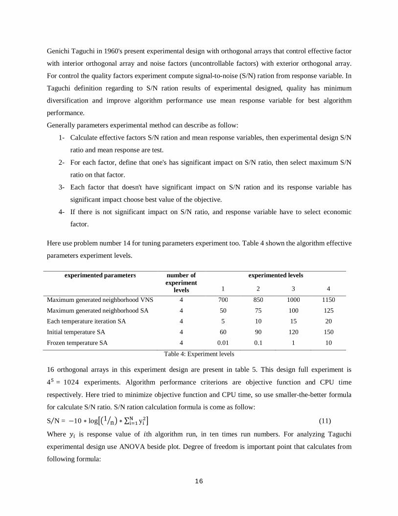
Here use problem number 14 for tuning parameters experiment too. Table 4 shown the algorithm effective

parameters experiment levels.

experimented parameters number of experiment

levels

experimented levels

1 2 3 4

Maximum generated neighborhood VNS 4 700 850 1000 1150

Maximum generated neighborhood SA 4 50 75 100 125 Each temperature iteration SA 4 5 10 15 20

Initial temperature SA 4 60 90 120 150

Frozen temperature SA 4 0.01 0.1 1 10

Table 4: Experiment levels 16 orthogonal arrays in this experiment design are present in table 5. This design full experiment is 4 = 1024 experiments. Algorithm performance criterions are objective function and CPU time

respectively. Here tried to minimize objective function and CPU time, so use smaller-the-better formula

for calculate S/N ratio. S/N ration calculation formula is come as follow: S N⁄ = −10 ∗ log 1 n ∗ ∑ y (11)

Where is response value of th algorithm run, in ten times run numbers. For analyzing Taguchi

experimental design use ANOVA beside plot. Degree of freedom is important point that calculates from

following formula:

17

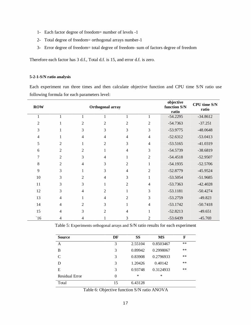
1- Each factor degree of freedom= number of levels -1

2- Total degree of freedom= orthogonal arrays number-1

3- Error degree of freedom= total degree of freedom- sum of factors degree of freedom

Therefore each factor has 3 d.f., Total d.f. is 15, and error d.f. is zero.

5-2-1-S/N ratio analysis

Each experiment run three times and then calculate objective function and CPU time S/N ratio use

following formula for each parameters level:

ROW Orthogonal array objective

function S/N ratio

CPU time S/N ratio

1 1 1 1 1 1 -54.2295 -34.8612 2 1 2 2 2 2 -54.7363 -37.251

3 1 3 3 3 3 -53.9775 -48.0648

4 1 4 4 4 4 -52.6312 -53.0413

5 2 1 2 3 4 -53.5165 -41.0319 6 2 2 1 4 3 -54.5739 -38.6819

7 2 3 4 1 2 -54.4518 -52.9507

8 2 4 3 2 1 -54.1935 -52.5706

9 3 1 3 4 2 -52.8779 -45.9524 10 3 2 4 3 1 -53.5054 -51.9685

11 3 3 1 2 4 -53.7363 -42.4028

12 3 4 2 1 3 -53.1181 -50.4274

13 4 1 4 2 3 -53.2759 -49.823 14 4 2 3 1 4 -53.1742 -50.7418

15 4 3 2 4 1 -52.8213 -49.651

`16 4 4 1 3 2 -53.6439 -45.769 Table 5: Experiments orthogonal arrays and S/N ratio results for each experiment

F MS SS DF Source ** 0.8503467 2.55104 3 A ** 0.2998067 0.89942 3 B ** 0.2796933 0.83908 3 C ** 0.40142 1.20426 3 D ** 0.3124933 0.93748 3 E * * 0 Residual Error 6.43128 15 Total

Table 6: Objective function S/N ratio ANOVA

18

S = ∑ F δ ∗ η (12)

A = ∑ (13)

F δ = 1 δ = i0 δ ≠ i (14) : Sum of S/N ratio on level th of the factor : factor level number in th experiment : S/N ratio of th experiment : total experiment number

S/N ratio results for each experiment are shown in table 5 too.

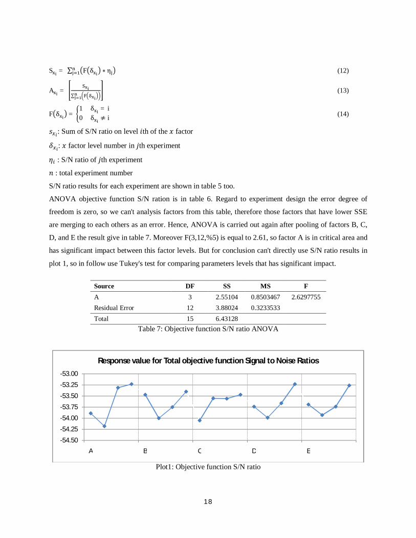
ANOVA objective function S/N ration is in table 6. Regard to experiment design the error degree of

freedom is zero, so we can't analysis factors from this table, therefore those factors that have lower SSE

are merging to each others as an error. Hence, ANOVA is carried out again after pooling of factors B, C,

D, and E the result give in table 7. Moreover F(3,12,%5) is equal to 2.61, so factor A is in critical area and

has significant impact between this factor levels. But for conclusion can't directly use S/N ratio results in

plot 1, so in follow use Tukey's test for comparing parameters levels that has significant impact.

F MS SS DF Source

2.6297755 0.8503467 2.55104 3 A

0.3233533 3.88024 12 Residual Error

6.43128 15 Total Table 7: Objective function S/N ratio ANOVA

Plot1: Objective function S/N ratio

-54.50

-54.25

-54.00

-53.75

-53.50

-53.25

-53.00

A B C D E

Response value for Total objective function Signal to Noise Ratios

19

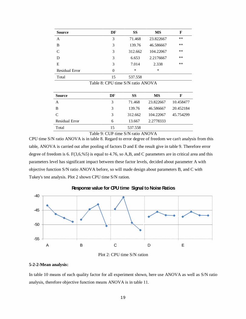
F MS SS DF Source ** 23.822667 71.468 3 A ** 46.586667 139.76 3 B ** 104.22067 312.662 3 C ** 2.2176667 6.653 3 D ** 2.338 7.014 3 E

* * 0 Residual Error

537.558 15 Total Table 8: CPU time S/N ratio ANOVA

F MS SS DF Source

10.458477 23.822667 71.468 3 A 20.452184 46.586667 139.76 3 B 45.754299 104.22067 312.662 3 C

2.2778333 13.667 6 Residual Error

537.558 15 Total Table 9: CUP time S/N ratio ANOVA

CPU time S/N ratio ANOVA is in table 8. Regard to error degree of freedom we can't analysis from this

table, ANOVA is carried out after pooling of factors D and E the result give in table 9. Therefore error

degree of freedom is 6. F(3,6,%5) is equal to 4.76, so A,B, and C parameters are in critical area and this

parameters level has significant impact between these factor levels, decided about parameter A with

objective function S/N ratio ANOVA before, so will made design about parameters B, and C with

Tukey's test analysis. Plot 2 shown CPU time S/N ration.

Plot 2: CPU time S/N ration

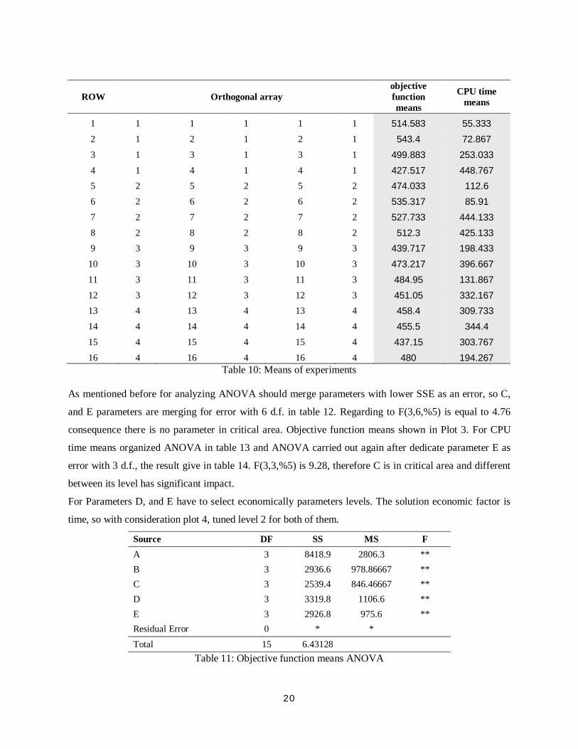
5-2-2-Mean analysis:

In table 10 means of each quality factor for all experiment shown, here use ANOVA as well as S/N ratio

analysis, therefore objective function means ANOVA is in table 11.

-55

-50

-45

-40

A B C D E

Response value for CPU time Signal to Noise Ratios

20

ROW Orthogonal array objective function means

CPU time means

1 1 1 1 1 1 514.583 55.333 2 1 2 1 2 1 543.4 72.867 3 1 3 1 3 1 499.883 253.033 4 1 4 1 4 1 427.517 448.767 5 2 5 2 5 2 474.033 112.6 6 2 6 2 6 2 535.317 85.91 7 2 7 2 7 2 527.733 444.133 8 2 8 2 8 2 512.3 425.133 9 3 9 3 9 3 439.717 198.433 10 3 10 3 10 3 473.217 396.667 11 3 11 3 11 3 484.95 131.867 12 3 12 3 12 3 451.05 332.167 13 4 13 4 13 4 458.4 309.733 14 4 14 4 14 4 455.5 344.4 15 4 15 4 15 4 437.15 303.767 16 4 16 4 16 4 480 194.267

Table 10: Means of experiments

As mentioned before for analyzing ANOVA should merge parameters with lower SSE as an error, so C,

and E parameters are merging for error with 6 d.f. in table 12. Regarding to F(3,6,%5) is equal to 4.76

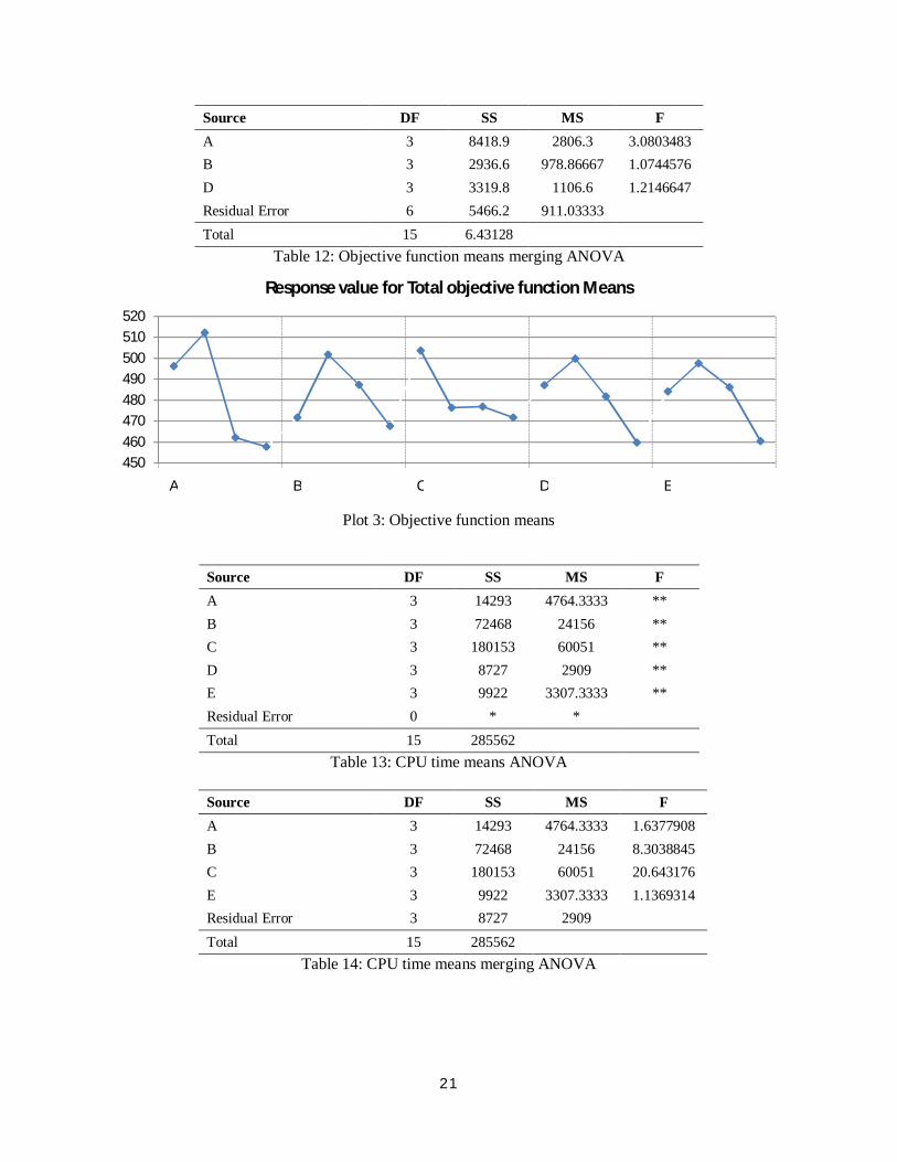
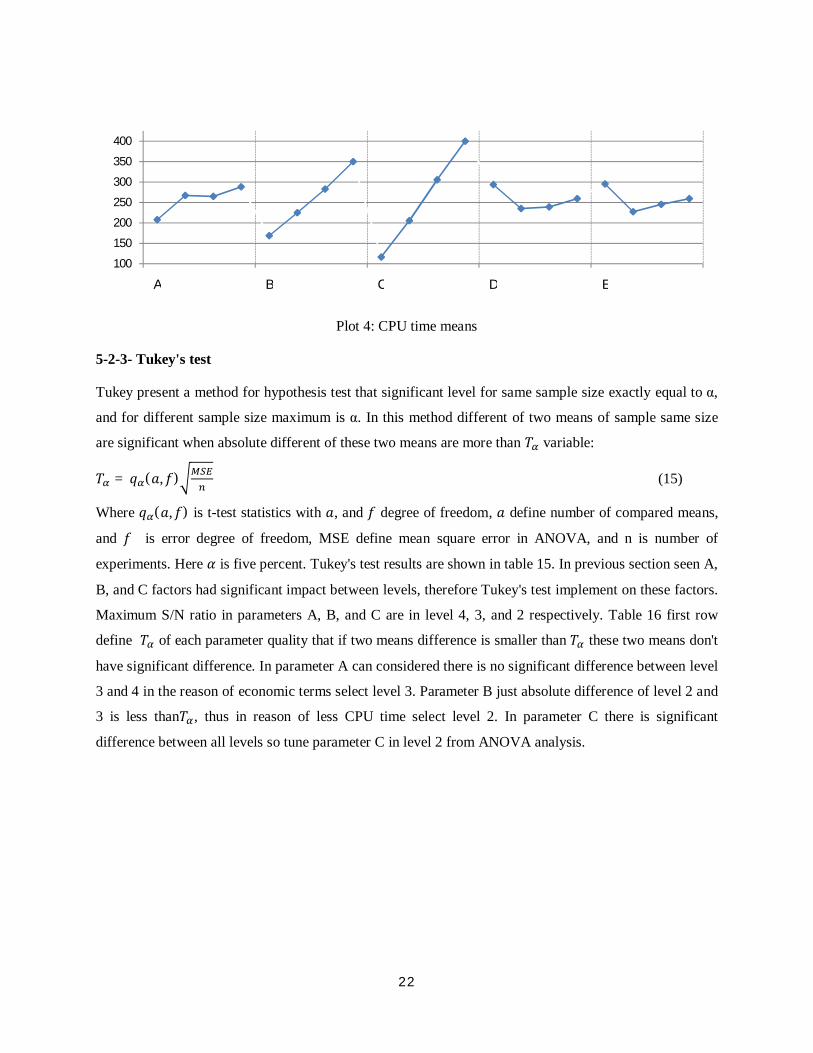
consequence there is no parameter in critical area. Objective function means shown in Plot 3. For CPU

time means organized ANOVA in table 13 and ANOVA carried out again after dedicate parameter E as

error with 3 d.f., the result give in table 14. F(3,3,%5) is 9.28, therefore C is in critical area and different

between its level has significant impact.

For Parameters D, and E have to select economically parameters levels. The solution economic factor is

time, so with consideration plot 4, tuned level 2 for both of them.

F MS SS DF Source ** 2806.3 8418.9 3 A ** 978.86667 2936.6 3 B ** 846.46667 2539.4 3 C ** 1106.6 3319.8 3 D ** 975.6 2926.8 3 E

* * 0 Residual Error

6.43128 15 Total Table 11: Objective function means ANOVA

21

F MS SS DF Source 3.0803483 2806.3 8418.9 3 A 1.0744576 978.86667 2936.6 3 B 1.2146647 1106.6 3319.8 3 D

911.03333 5466.2 6 Residual Error

6.43128 15 Total Table 12: Objective function means merging ANOVA

Plot 3: Objective function means

F MS SS DF Source ** 4764.3333 14293 3 A ** 24156 72468 3 B ** 60051 180153 3 C ** 2909 8727 3 D ** 3307.3333 9922 3 E

* * 0 Residual Error

285562 15 Total Table 13: CPU time means ANOVA

Table 14: CPU time means merging ANOVA

450460470480490500510520

A B C D E

Response value for Total objective function Means

F MS SS DF Source 1.6377908 4764.3333 14293 3 A 8.3038845 24156 72468 3 B 20.643176 60051 180153 3 C 1.1369314 3307.3333 9922 3 E

2909 8727 3 Residual Error

285562 15 Total

22

Plot 4: CPU time means

5-2-3- Tukey's test

Tukey present a method for hypothesis test that significant level for same sample size exactly equal to α,

and for different sample size maximum is α. In this method different of two means of sample same size

are significant when absolute different of these two means are more than variable: = ( , ) (15)

Where ( , ) is t-test statistics with , and degree of freedom, define number of compared means,

and is error degree of freedom, MSE define mean square error in ANOVA, and n is number of

experiments. Here is five percent. Tukey's test results are shown in table 15. In previous section seen A,

B, and C factors had significant impact between levels, therefore Tukey's test implement on these factors.

Maximum S/N ratio in parameters A, B, and C are in level 4, 3, and 2 respectively. Table 16 first row

define of each parameter quality that if two means difference is smaller than these two means don't

have significant difference. In parameter A can considered there is no significant difference between level

3 and 4 in the reason of economic terms select level 3. Parameter B just absolute difference of level 2 and

3 is less than , thus in reason of less CPU time select level 2. In parameter C there is significant

difference between all levels so tune parameter C in level 2 from ANOVA analysis.

100

150

200

250

300

350

400

A B C D E

23

Parameter A Parameter B Parameter C 1.84883 1.84883 0.597074 − -4.16 -3.61 0.29 − 4.74 -5.35 -0.58 − 7.36 2.18 -0.66 − 8.9 -1.74 -0.87 − 11.52 5.79 -0.95 − 2.62 7.53 -0.08

Table 15: Tukey's test results

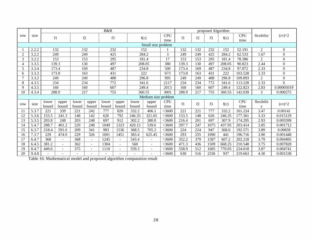
6- Computation results:

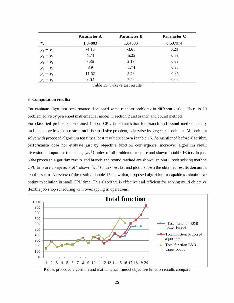
For evaluate algorithm performance developed some random problems in different scale. There is 20

problem solve by presented mathematical model in section 2 and branch and bound method.

For classified problems mentioned 1 hour CPU time restriction for branch and bound method, if any

problem solve less than restriction it is small size problem, otherwise its large size problem. All problem

solve with proposed algorithm ten times, best result are shown in table 16. As mentioned before algorithm

performance dose not evaluate just by objective function convergence, moreover algorithm result

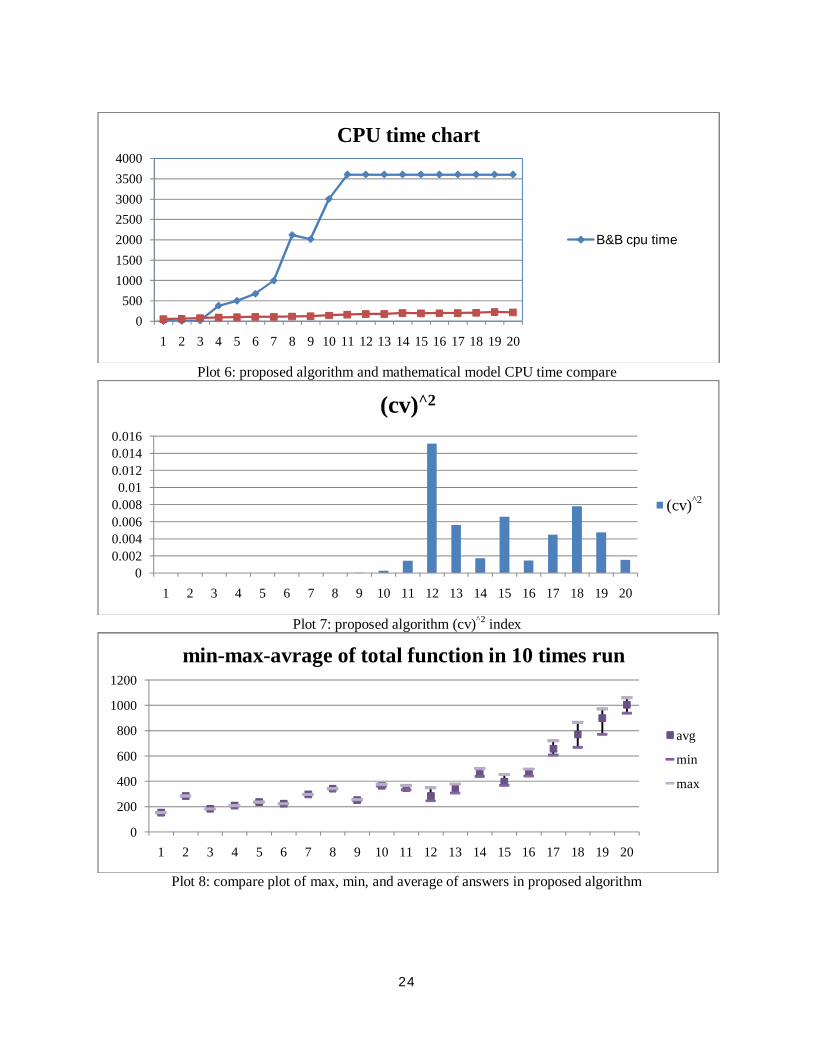
diversion is important too. Thus, ( ) index of all problems compute and shown in table 16 too. In plot

5 the proposed algorithm results and branch and bound method are shown. In plot 6 both solving method

CPU time are compare. Plot 7 shown ( ) index results, and plot 8 shown the obtained results domain in

ten times run. A review of the results in table 16 show that, proposed algorithm in capable to obtain near

optimum solution in small CPU time. This algorithm is effective and efficient for solving multi objective

flexible job shop scheduling with overlapping in operations.

Plot 5: proposed algorithm and mathematical model objective function results compare

0100200300400500600700800900

1000

1 2 3 4 5 6 7 8 9 10 11 12 13 14 15 16 17 18 19 20

Total function

- Total function B&B Lower boundTotal function Proposed algorithmTotal function B&B Upper bound

24

Plot 6: proposed algorithm and mathematical model CPU time compare

Plot 7: proposed algorithm (cv)^2 index

Plot 8: compare plot of max, min, and average of answers in proposed algorithm

0500

1000150020002500300035004000

1 2 3 4 5 6 7 8 9 10 11 12 13 14 15 16 17 18 19 20

CPU time chart

B&B cpu time

00.0020.0040.0060.0080.01

0.0120.0140.016

1 2 3 4 5 6 7 8 9 10 11 12 13 14 15 16 17 18 19 20

(cv)^2

(cv)^2

0

200

400

600

800

1000

1200

1 2 3 4 5 6 7 8 9 10 11 12 13 14 15 16 17 18 19 20

min-max-avrage of total function in 10 times run

avg

min

max

(cv)^2

25

7- Conclusion and future research

In this paper consider multiobjective flexible job shop scheduling with overlapping assumption.

Overlapping consumption is use full in many industrial among petrochemical and glass factories. Flexible

job shop scheduling problems are NP-Hard, therefore when overlapping in operation adds to problems

increase complexity, so flexible job shop problem with overlapping assumption is strongly NP-Hard.

Since these problems are in NP-Hard class can use Meta heuristic method for solving problems.

Decomposition approach in two stage and two different Meta heuristic algorithms are present in this

paper. Decomposition approach first stage is assignment, and second one is scheduling algorithms. Select

proper combination of SA and VNS algorithms with TOPSIS method. In this paper consider critical

machine work loading time, and total machine work loading time beside Makespan as scheduling

criterions. Moreover for improve proposed algorithm performance use Taguchi experimental design and

Tukey's test. Moreover in this paper mixed integer linear programming (MILP) present and solve with

branch and bound method then compare its results with proposed algorithm. Regarded to results proposed

algorithm is effective and efficient in small CPU time. Recommendations on future works are as follow.

Studying in filed of additional constraints, such as random breakdown and maintenance requirement,

optimize other objective function such as earliness and tardiness with developing Meta heuristics

algorithm. Consideration stochastic environment and setup sequence dependent time assumption are very

useful.

26

Reference: [1] Garey MR، Johnson، DS، Sethi R The complexity of flowshop and jobshop scheduling. Mathematics of Operations Research 1976;1:117-129 [2] Gen, M., Cheng, R. Genetic algorithm and engineering design, New York: John Wiley and Sons. 1997 [3] Gen, M., Cheng, R. Genetic algorithm and engineering design, New York: John Wiley and Sons. 2000 [4] Blazewicz, J., Domschke, W., Pesch, E. The job shop scheduling problem: conventional and new solution techniques, European journal of operational research 1996;93:1-33 [5] Bruker, P., Schlie, R. Job shop scheduling with multi-purpose machines. Computing, 1990;45, 369-375 [6] Xia W.، Wu Z. An effective hybrid optimization approach for multi-objective flexible jobshop scheduling problems. Computers & Industrial Engineering. 2005;48: 409–425 [7] Brandimarte، P. Routing and scheduling in a flexible job shop by taboo search. Annals of Operations Research 1993; 41، 157-183. [8] Tung, L. F., Li, L., Nagi, R. Multi-objective scheduling for the hierarchical control of flexible manufacturing systems. The international journal of flexible manufacturing systems 1999;11, 379-409. [9] Hurink, E., Jurisch, B.,Thole, M. Tabu search for the job shop scheduling problem with multi-purpose machine. Operations Research Spektrum 1994;15, 205-215 [10] Dauzere-Peres, S., & Paulli, J. An integrated approach for modeling and solving the general multiprocessor job shop scheduling problem using tabu search. Annals pf Operations Research 1997; 70, 281-306. [11] Mastrololli, M., & Gambardella, L. M. Effective neighborhood functions for the flexible job shop problem. Journal of scheduling 2002;3(1), 3-20. [12] Rigao, C. Tardiness minimization in a flexible job shop: A tabu search approach. Journal of Intelligent Manufacturing 2004;15(1), 103–115. [13] Kacem I.، Hammadi S.، Borne P. Pareto-optimality approach for flexible job-shop scheduling problems: hybridization of evolutionary algorithms and fuzzy logic. Mathematics and Computers in Simulation. 2002;60:245–276 [14] Zandieh, M., Mahdavi, I, Bagheri, A. Solving flexible job shop scheduling problems by a genetic algorithm, journal of applied sciences 2008; 8 (24): 4650-4655 [15] Gao، J.، Sun، L.،and Gen، M. A Hybrid genetic and variable neighborhood descent algorithm for flexible job shop scheduling problems. Computers & operations research 2008;35(9) ، 2892-2907 DOI: 10.1016/j.cor.2007.01.001. [16] Pezzella، F.، Morganti، G.، and Ciaschetti، G. A genetic algorithm for the flexible job shop scheduling problem. Computers & operations research 2008;35(10) ، 3202-3212 DOI: 10.1016/ j.cor.2007.02.014 [17] Alvarez-Valdes، R.، Fuertes، A.، Tamarit، J.M.، Gimenez، G.، Ramos، R.،s. A heuristic to schedule flexible job shop in a glass factory. European Journal of Operational Research 2005;165، 525-534 [18] Fattahi P.، Jolai F.، Arkat J. Flexible job shop scheduling with overlapping in operations، Appl. Math. Modelling doi: 2008;10.1016/j.apm.2008.10.029 [19] Zhang, G, Shao, X, Li, p, Gao , L. An effective hybrid particle swarm optimization algorithm for multi-objective flexible job-shop scheduling problem; Computers & Industrial Engineering 2008; Volume 56, Issue 4, May 2009, Pages 1309-1318 [20] Xing, L., Chen، Y., Yang, K. Multi-objective flexible job shop schedule: Design and evaluation by simulation modeling. Applied Soft Computing 2009; 9 362–376 [21] Hansen, P., Mladenovic´, N. Variable neighborhood search: Principles and applications. European Journal of Operations Research 2001;130 (3), 449–467. [22] Garcia CG, Dionisio PB, Campos V, Marti R. Variable neighborhood search for the linear ordering problem, Computers & Operations Research 2006;33: 3549–3565.

27

[23] Aarts, E., Korst, J. Simulated Annealing and Boltzmann machine, A stochastic approach to computing. Chichester: John Wiley and Sons 1989 [24] Pincus M. A monte carlo method for the approximate solution of certain type of constrained optimization problems, operations research 1970; 18, 1225-1228 [25] Yazdani, M. Amiri, M. Zandieh, M. Flexible job-shop scheduling with parallel variable neighborhood search algorithm Expert Systems with Applications, 2010;Volume 37, Issue 1, January, Pages 678-687

28

row size B&B proposed Algorithm

flexibility (cv)^2 f1 f2 f3 f(c) CPU time f1 f2 f3 f(c) CPU

time Small size problem

1 2.2.2 132 132 232 152 1 132 132 232 152 52.191 2 0 2 3.2.2 249 249 425 284.2 3 249 249 425 284.2 62.533 1.67 0 3 3.2.2 153 153 295 181.4 17 153 153 295 181.4 78.386 2 0 4 3.3.5 139.3 130 497 208.05 380 139.3 130 497 208.05 90.823 2.44 0 5 3.3.4 173.4 169 487 234.8 500 173.4 169 487 234.8 97.872 2.33 0 6 3.3.3 173.8 163 431 222 673 173.8 163 431 222 103.528 2.33 0 7 3.3.2 249 249 488 296.8 995 249 249 488 296.8 109.893 2 0 8 4.3.5 234 234 772 341.6 2117 234 234 772 341.6 113.228 2.33 0 9 4.3.5 160 160 607 249.4 2013 160 160 607 249.4 122.823 2.83 0.00005019 10 4.3.4 288.9 217 755 360.55 3001 288.9 217 755 360.55 142.039 3 0.000275

Medium size problem

row size lower bound

upper bound

lower bound

upper bound

lower bound

upper bound

lower bound

upper bound

CPU time f1 f2 f3 f(c) CPU

time flexibilit

y (cv)^2

11 5.3.7 221 339 221 242 777 820 332.2 406.1 <3600 221 221 777 332.2 161.224 3.47 0.00141 12 5.3.6 153.5 241.3 148 142 626 792 246.35 321.65 <3600 153.5 148 626 246.35 177.361 3.33 0.015129 13 5.3.5 203.8 248 203 248 697 912 302.2 380.8 <3600 216.4 201 697 307.9 174.295 2.93 0.005599 14 5.4.7 288.7 401.2 220 248 1049 1323 420.15 539.6 <3600 297.7 247 1075 437.95 203.414 3.85 0.001712 15 6.3.7 218.4 591.6 209 341 983 1536 368.5 705.3 <3600 224 224 947 368.6 192.571 3.89 0.00659 16 7.3.7 229 474.9 229 326 1001 1451 383.4 625.45 <3600 293 255 1090 441 196.716 3.90 0.001448 17 6.4.7 368 - 368 - 1245 - 543.4 - <3600 352.2 379 1587 607.2 202.218 3.79 0.004495 18 6.4.5 381.2 - 362 - 1304 - 560 - <3600 471.3 436 1509 668.25 210.548 3.75 0.007828 19 8.4.7 449.6 - 375 - 1110 - 559.3 - <3600 558.9 512 1685 770.05 224.018 3.87 0.004741 20 9.4.8 - - - - - - - - <3600 630 516 2336 937 219.663 4.30 0.001538

Table 16: Mathematical model and proposed algorithm computation result